Hidden Gibbs random fields model selection using Block Likelihood Information Criterion

Abstract

Performing model selection between Gibbs random fields is a very challenging task. Indeed, due to the Markovian dependence structure, the normalizing constant of the fields cannot be computed using standard analytical or numerical methods. Furthermore, such unobserved fields cannot be integrated out and the likelihood evaluztion is a doubly intractable problem. This forms a central issue to pick the model that best fits an observed data. We introduce a new approximate version of the Bayesian Information Criterion. We partition the lattice into continuous rectangular blocks and we approximate the probability measure of the hidden Gibbs field by the product of some Gibbs distributions over the blocks. On that basis, we estimate the likelihood and derive the Block Likelihood Information Criterion (BLIC) that answers model choice questions such as the selection of the dependency structure or the number of latent states. We study the performances of BLIC for those questions. In addition, we present a comparison with ABC algorithms to point out that the novel criterion offers a better trade-off between time efficiency and reliable results.

Keywords: Hidden Markov random fields; model selection; Bayesian Information Criterion

1 Introduction

Gibbs or discrete Markov random fields have appeared as convenient statistical model to analyse different types of spatially correlated data. Notable examples are the autologistic model (Besag,, 1974) and its extension the Potts model used to describe the spatial dependency of discrete random variables (e.g., shades of grey or colors) on the vertices of an undirected graph (e.g., a regular grid of pixels). In particular, hidden Markov random fields offer an appropriate representation for practical settings where the true state is unknown. The general framework can be described as an observed data $\mathbf{y}$ which is a noisy or incomplete version of an unobserved discrete latent process $\mathbf{x}$. Shaped by the development of Geman and Geman, (1984) and Besag, (1986), these models have enjoyed great success in image analysis – see for example Alfò et al., (2008) and Moores et al., (2014) who performed image segmentation with the help of this modelling – but also in other applications including disease mapping (e.g., Green and Richardson,, 2002) and genetic analysis (e.g., François et al.,, 2006, Friel et al.,, 2009) to name a few. Despite their popularity, Gibbs random fields suffer from major computational difficulties since their normalizing constant is intractable. This forms a central issue in statistical analysis as the computation of the likelihood is an integral part of the procedure for both parameter inference (e.g., Celeux et al.,, 2003, Friel et al.,, 2009, McGrory et al.,, 2009, Everitt,, 2012) and model selection (e.g., Grelaud et al.,, 2009, Friel,, 2013, Cucala and Marin,, 2013, Stoehr et al.,, 2015). Remark the exception of small latices on which we can apply the recursive algorithm of Reeves and Pettitt, (2004), Friel and Rue, (2007) and obtain an exact computation of the normalizing constant. However, the complexity in time of the above algorithm grows exponentially and is thus helpless on large lattices.

The present paper cares about the problem of selecting the number of latent states as well as the dependency structure of hidden Potts model and explores the opportunity of using the Bayesian Information Criterion (BIC, Schwarz,, 1978) to answer the question. If the problem of recovering the number of hidden states is common in image segmentation, the problem of selecting a dependency structure has received little attention in the literature. Stoehr et al., (2015) have proposed to use approximate Bayesian computation (ABC) model choice (e.g., Marin et al.,, 2012) based on geometric summary statistics to tackle the choice of an underlying graph but their approach is restricted to the latter. While our work is motivated by a more general issue, it offers a way to overcome the computational burden of ABC algorithms.

Model choice is a problem of probabilistic model comparison. The standard approach to compare one model against another is based on the Bayes factor (Kass and Raftery,, 1995) that involves the ratio of the evidence of each model. However the evidence can usually not be computed with standard procedure due to a high-dimensional integral. Various approximations have been proposed but a commonly used one, if only for its simplicity, is BIC that is an asymptotic estimate of the evidence based on the Laplace method for integrals. The criterion is a simple penalized function of the maximized log-likelihood which, in the context of hidden Gibbs random fields, cannot be computed since it requires to integrate the intractable Gibbs distribution over the latent space configurations. As regards the simpler case of observed Markov random field solutions have been brought by penalized pseudolikelihood (Ji and Seymour,, 1996) or MCMC approximation of BIC (Seymour and Ji,, 1996). To circumvent the computational difficulties in the hidden case, little has been done before the work of Stanford and Raftery, (2002) and Forbes and Peyrard, (2003). Both propose approximations that consist in replacing the intractable likelihood with a product distribution on system of independent variables to make the computation tractable. Our main contribution is to show that larger collections of variables, namely blocks of the lattice, can be considered by taking advantage of the exact recursion of Reeves and Pettitt, (2004) and leads to an efficient criterion : the Block Likelihood Information Criterion (BLIC). In particular, we will show that a reasonable approximation of the Gibbs distribution is a product of Gibbs distributions on each independent block. Such ideas have occurred in the context of composite likelihood but the use of non-genuine probability distribution results in misspecified model (e.g., Okabayashi et al.,, 2011, Friel,, 2012, Stoehr and Friel,, 2015) that we have decided to avoid.

The paper is organized as follows: Section 2 presents hidden Gibbs random fields. In section 3, after recalling the basis of BIC, we introduced our Block Likelihood Information Criterion (BLIC). In Section 4, to assess the performances of the novel criterion, it is compared to pre-existing criteria on simulated data sets. We fill in our study with a comparison between BLIC and the ABC algorithm of Stoehr et al., (2015).

2 Hidden Gibbs random fields

A discrete random field $\mathbf{X}$ is a collection of random variables $X_{i}$ indexed by a finite set $\mathscr{S}=\{1,\dots,n\}$, whose elements are called sites, and taking values in a finite state space $\mathscr{X}:=\{0,\ldots,K-1\}$, interpreted as colors. For a given subset $A\subset\mathscr{S}$, $\mathbf{X}_{A}$ and $\mathbf{x}_{A}$ respectively define the random process on $A$, i.e., $\{X_{i},i\in A\}$, and a realisation of $\mathbf{X}_{A}$. Denotes $\mathscr{S}\setminus A=-A$ the complement of $A$ in $\mathscr{S}$. When modeling a digital image, the sites are lying on a regular 2D-grid of pixels, and their dependency is given by an undirected graph $\mathscr{G}$ which induces a topology on $\mathscr{S}$: by definition, sites $i$ and $j$ are adjacent or neighbor if and only if $i$ and $j$ are linked by an edge in $\mathscr{G}$. A random field $\mathbf{X}$ is a Markov random field with respect to $\mathscr{G}$, if for all configuration $\mathbf{x}$ and for all sites $i$

$$\mathbf{P}\left(X_{i}=x_{i}\;|\;\mathbf{X}_{-i}=\mathbf{x}_{-i}\right)=\mathbf{P}\left(X_{i}=x_{i}\;|\;\mathbf{X}_{\mathscr{N}(i)}=\mathbf{x}_{\mathscr{N}(i)}\right),$$ (1)

where $\mathscr{N}(i)$ denotes the set of all the adjacent sites to $i$ in $\mathscr{G}$. The Hammersley-Clifford theorem states that if the distribution of a Markov random field with respect to a graph $\mathscr{G}$ is positive for all configuration $\mathbf{x}$ then it admits a Gibbs representation for the same topology (see for example Grimmett, (1973), Besag, (1974) and for a historical perspective Clifford, (1990)), namely a probability measure $\pi$ on $\mathscr{X}^{n}$ given by

$$\pi\left(\mathbf{x}\;|\;\psi,\mathscr{G}\right)=\frac{1}{Z\left(\psi,\mathscr{G}\right)}\exp\left\{-H\left(\mathbf{x}\;|\;\psi,\mathscr{G}\right)\right\},$$ (2)

where $\psi=(\psi_{1},\ldots,\psi_{d})$ is a vector of parameters, $H$ denotes the energy function or Hamiltonian. The present paper solely focuses on models whose Hamiltonian linearly depends on the parameter $\psi$, that is

$$H\left(\mathbf{x}\;|\;\psi,\mathscr{G}\right)=-\psi^{T}\mathbf{S}(\mathbf{x}).$$

where $\mathbf{S}(\mathbf{x})=(s_{1}(\mathbf{x}),\ldots,s_{d}(\mathbf{x}))$ is a vector of sufficient statistics. The inherent difficulty of all these models that arises from the intractable normalizing constant, called the partition function, defined by

$$Z(\psi,\mathscr{G})=\sum_{\mathbf{x}\in\mathscr{X}^{n}}\exp\left\{\psi^{T}\mathbf{S}(\mathbf{x})\right\}$$

The latter is a summation over the numerous possible realizations of the random field $\mathbf{X}$, that cannot be computed directly (except for small grids and small number of colors $K$).

In hidden Markov random fields, the latent process is observed indirectly through another field; this permits the modelling of noise that may happen upon many concrete situations. The aim is to infer some properties of a latent state $\mathbf{x}$ given an observation $\mathbf{y}$. Precisely, given the realization $\mathbf{x}$ of the latent, the observation $\mathbf{y}$ is a family of random variables indexed by the set of sites $\mathscr{S}$, and taking values in a set $\mathscr{Y}$, i.e., $\mathbf{y}=\left\{y_{i};{i\in\mathscr{S}}\right\}$, and are commonly assumed as independent draws that form a noisy version of the hidden field. Consequently, we set the conditional distribution of $\mathbf{Y}$ knowing $\mathbf{X}=\mathbf{x}$, also called emission distribution, as the product

$$\pi\left(\mathbf{y}\;|\;\mathbf{x},\phi\right)=\prod_{i\in\mathscr{S}}\pi\left(y_{i}\;|\;x_{i},\phi\right),$$

where $\pi(y_{i}\mid x_{i},\phi)$ is the marginal noise distribution parametrized by $\phi$, that is given for any site $i$. Those marginal distributions are for instance discrete distributions (Everitt,, 2012), Gaussian (e.g., Besag et al.,, 1991, Qian and Titterington,, 1991, Forbes and Peyrard,, 2003, Cucala and Marin,, 2013) or Poisson distributions (e.g., Besag et al.,, 1991). Model of noise that takes into account information of the nearest neighbors have also been explored (Besag,, 1986). Hence the likelihood of the hidden Gibbs random field with parameter $\psi$ on the graph $\mathscr{G}$ and emission distribution $\pi\left(\cdot\;|\;\mathbf{x},\phi\right)$ is given by

$$\pi\left(\mathbf{y}\;|\;\phi,\psi\right)=\sum_{\mathscr{X}^{n}}\pi\left(\mathbf{y}\;|\;\mathbf{x},\phi\right)\pi\left(\mathbf{x}\;|\;\psi,\mathscr{G}\right).$$ (3)

The latter faces a double intractable issue as neither the likelihood of the latent field, nor the above sum can be computed directly: the cardinality of the range of the sum is of combinatorial complexity.

3 Block Likelihood Information Criterion

The Bayesian Information Criterion offers a mean arising from Bayesian viewpoint to select a statistical model. In what follows, we provide solely the foundation that motivates our contribution and we refer the reader for instance to Raftery, (1995) for a more detailed presentation.

3.1 Background on Bayesian Information Criterion

We are given $n$ independent and identically distributed observations $\mathbf{y}=\left\{y_{1},\ldots,y_{n}\right\}$ from an unknown statistical model to estimate. The Bayesian approach to model selection is based on posterior model probabilities. Consider a finite set of models $\left\{m:1,\ldots,M\right\}$ where each one is defined by a probability density function $\pi_{m}$ related to a parameter space $\Theta_{m}$. The model that best fits an observation $\mathbf{y}$ is the model with the highest posterior probability

$$\pi\left(m\;|\;\mathbf{y}\right)=\frac{\pi(m)e\left(\mathbf{y}\;|\;m\right)}{\sum_{m^{\prime}}\pi(m^{\prime})e\left(\mathbf{y}\;|\;m^{\prime}\right)},$$

where $e\left(\mathbf{y}\;|\;m\right)$ denotes the evidence of $m$, that is the joint distribution of $(\mathbf{y},\theta_{m})$ integrated over space parameter $\Theta_{m}$

$$e\left(\mathbf{y}\;|\;m\right)=\int\pi_{m}\left(\mathbf{y}\;|\;\theta_{m}\right)\pi_{m}\left(\theta_{m}\right)\mathrm{d}\theta_{m}.$$

Under the assumption of model being equally likely a priori, it is equivalent to choose the model with the largest evidence. From the Laplace method for integrals, under regularity conditions, the evidence of model $m$ can be written as

$$\log e\left(\mathbf{y}\;|\;m\right)=\log\pi_{m}\left(\mathbf{y}\;|\;\hat{\theta}_{\text{MLE}}\right)-d_{m}\log(n)+R_{m}\left(\hat{\theta}_{\text{MLE}}\right)+\operatorname*{\mathcal{O}}\left(n^{-\frac{1}{2}}\right),$$ (4)

where where $\hat{\theta}_{\text{MLE}}$ is the maximum likelihood estimator of $\pi_{m}$, $d_{m}$ is the number of free parameters for model $m$ and $R_{m}$ is bounded as the sample size grows to infinity (e.g., Schwarz,, 1978, Tierney and Kadane,, 1986).

BIC is an asymptotical estimate of the evidence defined by

$$-2\log e\left(\mathbf{y}\;|\;m\right)\simeq\text{BIC}(m)=-2\log\pi_{m}\left(\mathbf{y}\;|\;\hat{\theta}_{\text{MLE}}\right)+d_{m}\log(n).$$ (5)

The $d_{m}\log(n)$ term corresponds to a penalty term which increases with the complexity of the model. Thus selecting the model with the largest evidence is equivalent to choose the model which minimizes BIC. Regardless of the prior on parameter, the error in (5) is, in general, solely bounded and does not go to zero even with an infinite amount of data. The approximation may hence seem somewhat crude. However as observed by Kass and Raftery, (1995) the criterion does not appear to be qualitatively misleading as long as the sample size $n$ is much larger than the number $d_{m}$ of free parameters in the model. In addition, a reasonable choice of the prior can lead to much smaller error. Indeed, Kass and Wasserman, (1995) have found that the error is $\operatorname*{\mathcal{O}}\left(n^{-1/2}\right)$ for a well chosen multivariate normal prior distribution.

BIC can be defined beside the special case of independent random variables. In the latter case the number of free parameter is, in general, not equal to the dimension of the parameter space as for the independent case. The consistency of BIC has been proven in various situations such as independent and identically distributed processes from the exponential families (Haughton,, 1988), mixture models (Keribin,, 2000), Markov chains (Csiszár et al.,, 2000, Gassiat,, 2002). When dealing with observed Markov random fields, aside from the problem of intractable likelihoods the number of free parameters in the penalty term has no simple formula. In the context of selecting a neighborhood system, Csiszár and Talata, (2006) proposed to replace the likelihood by the pseudolikelihood (Besag,, 1975) and modify the penalty term as the number of all possible configurations for the neighboring sites. The resulting criterion is shown to be consistent as regards this model choice. Up to our knowledge such a result has not been yet derived for hidden Markov random field. The problem of approximating BIC could be termed a triple intractable problem since neither the maximum likelihood estimate $\hat{\theta}_{\text{MLE}}$ nor the incomplete likelihood $\pi_{m}(\cdot\mid\theta)$ can be computed with standard methods since they require to integrate over the latent configuration space and no simple definition of $d_{m}$ is available.

3.2 Gibbs distribution approximations

A convenient way to circumvent the issues of computing BIC is to replace the Gibbs distribution by tractable surrogates since it avoids the use of time consuming simulations methods. As for the pseudolikelihood (Besag,, 1975) and more generally composite likelihood (Lindsay,, 1988), the main idea consists in replacing the original Markov distribution by a product of easily normalized distribution. But while composite likelihoods are not a genuine probability distribution for Gibbs random field, the focus hereafter is solely on valid probability function by considering system of independent variables. This choice is motivated by the observations that at finite sample size, when dealing with composite likelihood, misspecification of the model has to be taken into account (e.g., Friel,, 2012, Stoehr and Friel,, 2015), so that constant terms may appear in the remainder $R_{m}$ in (4).

Finding good approximations of the Gibbs distribution has long standing antecedents in statistical mechanics when one aims at predicting the response to the system to a change in the Hamiltonian. One important technique is based on a variational approach as the minimizer of the free energy, sometimes referred to as variational or Gibbs free energy and defined with the Kullback-Leibler divergence between $\mathbf{P}$ and the target distribution $\pi(\cdot\mid\psi,\mathscr{G})$ as

$$F(\mathbf{P})=-\log Z\left(\psi,\mathscr{G}\right)+\text{KL}\left(\mathbf{P},\pi(\cdot\mid\psi,\mathscr{G})\right).$$ (6)

The Kullback-Leibler divergence being non-negative and zero if and only if $\mathbf{P}=\pi(\cdot\mid\psi,\mathscr{G})$, the free energy has an optimal lower bound achieved for $\mathbf{P}=\pi(\cdot\mid\psi,\mathscr{G})$. Minimizing the free energy with respect to the set of probability distribution on $\mathscr{X}^{n}$ allows to recover the Gibbs distribution but presents the same computational intractability. A solution is to minimize the Kullback-Leibler divergence over a restricted class of tractable probability distribution on $\mathscr{X}^{n}$. This is the basis of mean field approaches that aim at minimizing the Kullback-Leibler divergence over the set of probability functions that factorize on sites of the lattice. The minimization of (6) over this set leads to fixed point equations for each marginal of $\mathbf{P}$ (see for example Jordan et al.,, 1999). The resulting solution motivates the mean field-like approximations of Celeux et al., (2003) for which the neighbors of a site $i$ are set to well chosen constant independently of the value at the given site, namely

$$\mathbf{P}^{\text{MF-like}}\left(\mathbf{x}\;|\;\psi,\mathscr{G}\right)=\prod_{i\in\mathscr{S}}\pi\left(x_{i}\;|\;\mathbf{X}_{\mathscr{N}(i)}=\tilde{\mathbf{x}}_{\mathscr{N}(i)},\psi,\mathscr{G}\right).$$ (7)

Instead of considering distributions that completely factorize on single sites, we are hereafter interested in tractable approximations that factorize over larger sets of nodes, namely blocks of the lattice. Consider a partition of $\mathscr{S}$ into contiguous rectangular blocks, namely

$$\mathscr{S}=\bigsqcup_{\ell=1}^{C}A(\ell),$$

and denote $\tilde{D}$ the class of independent probability distributions $\mathbf{P}$ that factorize with respect to this partition, that is if $\mathscr{X}^{n}_{A(\ell)}$ stands for the configuration space of the block $A(\ell)$, for all $\mathbf{x}$ in $\mathscr{X}^{n}$

$$\mathbf{P}(\mathbf{x})=\prod_{\ell=1}^{C}\mathbf{P}_{\ell}\left(x_{A(\ell)}\right),\text{ where }\mathbf{P}_{\ell}\in\mathcal{M}_{1}^{+}\left(\mathscr{X}^{n}_{A(\ell)}\right)\text{ and }\mathbf{P}\in\mathcal{M}_{1}^{+}(\mathscr{X}^{n}).$$

To take over from the Gibbs likelihood, we propose to explore the opportunity of probability distributions in $\tilde{D}$ of the form

$$\mathbf{P}\left(\mathbf{x}\;|\;\tilde{\mathbf{x}},A(1),\ldots,A(C),\psi\right)=\prod_{\ell=1}^{C}\pi\left(\mathbf{x}_{A(\ell)}\;|\;\mathbf{X}_{B(\ell)}=\tilde{\mathbf{x}}_{B(\ell)},\psi,\mathscr{G}\right),$$ (8)

where $\tilde{\mathbf{x}}$ is a constant field in $\mathscr{X}^{n}$ to specify and $B(\ell)$ is either the border of $A(\ell)$, i.e., elements of the absolute complement of $A(\ell)$ that are connected to elements of $A(\ell)$ in $\mathscr{G}$, or the empty set. In the latter case, we are cancelling the edges in $\mathscr{G}$ that link elements of $A(\ell)$ to elements of any other subset of $\mathscr{S}$ such that the factorization is independent of $\tilde{\mathbf{x}}$. The Gibbs distribution is then simply replaced by the product of the likelihood restricted to $A(\ell)$. For instance a Potts model on $\mathscr{X}^{n}$ is replaced with a product of Potts models on $\mathscr{X}^{n}_{A(\ell)}$. To underline that point, $\tilde{\mathbf{x}}$ is omitted in what follows when $B(\ell)=\emptyset$. Note that composite likelihoods differs from (8) in most cases since blocks are not allowed to overlap and contrary to conditional composite likelihoods, neighbors are set to constants. The only example of composite likelihoods that lies in $\tilde{D}$ is marginal composite likelihoods for non overlapping blocks.

The assumption of independent blocks leads to tractable BIC approximations. Indeed, plugging the probability distribution (8) in place of the Gibbs distribution in (3) yields

$$\mathbf{P}_{m}\left(\mathbf{y}\;|\;\tilde{\mathbf{x}},\theta\right) =\sum_{\mathbf{x}\in\mathscr{X}^{n}}\pi\left(\mathbf{y}\;|\;\mathbf{x},\phi\right)\mathbf{P}\left(\mathbf{x}\;|\;\tilde{\mathbf{x}},A(1),\ldots,A(C),\psi\right)$$

$$=\prod_{\ell=1}^{C}~{}\sum_{\mathbf{x}_{A(\ell)}}\left\{\prod_{i\in A(\ell)}\pi\left(y_{i}\;|\;x_{i},\phi\right)\right\}\pi\left(\mathbf{x}_{A(\ell)}\;|\;\mathbf{X}_{B(\ell)}=\tilde{\mathbf{x}}_{B(\ell)},\psi,\mathscr{G}\right)$$

$$=\prod_{\ell=1}^{C}\sum_{\mathbf{x}_{A(\ell)}}\pi\left(\mathbf{y}_{A(\ell)}\;|\;\mathbf{x}_{A(\ell)},\phi\right)\pi\left(\mathbf{x}_{A(\ell)}\;|\;\mathbf{X}_{B(\ell)}=\tilde{\mathbf{x}}_{B(\ell)},\psi,\mathscr{G}\right).$$ (9)

This estimate of the incomplete likelihood $\pi_{m}(\cdot\mid\theta)$ leads to the following BIC approximations

$$\text{BIC}(m)\approx-2\log\mathbf{P}_{m}\left(\mathbf{y}\;|\;\tilde{\mathbf{x}},\theta^{\ast}\right)+d_{m}\log(|\mathscr{S}|):=\text{BLIC}^{~{}\tilde{\mathbf{x}}}\left(m\;|\;\theta^{\ast}\right),$$ (10)

where $\theta^{\ast}=\left(\phi^{\ast},\psi^{\ast}\right)$ is a parameter value to specify. We refer to these approximations as Block Likelihood Information Criterion (BLIC). In the first instance, the number of free parameters $d_{m}$ is set to the dimension of $\Theta_{m}$, that is we are neglecting the interaction between variables within a block in the penalty term.

Our proposal relies on that each term of the product (9) can be computed using the recursion of Friel and Rue, (2007) as long as the blocks are small enough. Indeed for models whose potential linearly depends on the parameter, the probability distribution on $A(\ell)$ can be written as a Gibbs distribution on the block conditioned on the fixed border $\tilde{\mathbf{x}}_{B(\ell)}$, namely

$$\pi\left(\mathbf{x}_{A(\ell)}\;|\;\mathbf{X}_{B(\ell)}=\tilde{\mathbf{x}}_{B(\ell)},\psi,\mathscr{G}\right)=\frac{1}{Z\left(\psi,\mathscr{G},\tilde{\mathbf{x}}_{B(\ell)}\right)}\exp\left\{\psi^{T}\mathbf{S}\left(\mathbf{x}_{A(\ell)}\;|\;\tilde{\mathbf{x}}\right)\right\},$$

where $\mathbf{S}\left(\mathbf{x}_{A(\ell)}\;|\;\tilde{x}\right)$ is the restriction of $\mathbf{S}$ to the subgraph defined on the set $A(\ell)$ and conditioned on the fixed border $\tilde{\mathbf{x}}_{B(\ell)}$, and $Z\left(\psi,\mathscr{G},\tilde{\mathbf{x}}_{B(\ell)}\right)$ is the corresponding normalizing constant. Assuming that all the marginals of the emission distribution are positive, it follows

$$\sum_{\mathbf{x}_{A(\ell)}}\pi\left(\mathbf{y}_{A(\ell)}\;|\;\mathbf{x}_{A(\ell)},\phi\right)\pi\left(\mathbf{x}_{A(\ell)}\;|\;\mathbf{X}_{B(\ell)}=\tilde{\mathbf{x}}_{B(\ell)},\psi,\mathscr{G}\right)\\ =\frac{1}{Z\left(\psi,\mathscr{G},\tilde{\mathbf{x}}_{B(\ell)}\right)}\underbrace{\sum_{\mathbf{x}_{A(\ell)}}\exp\left\{\log\pi\left(\mathbf{y}_{A(\ell)}\;|\;\mathbf{x}_{A(\ell)},\phi\right)+\psi^{T}\mathbf{S}\left(\mathbf{x}_{A(\ell)}\;|\;\tilde{\mathbf{x}}\right)\right\}}_{=Z\left(\theta,\mathscr{G},\mathbf{y}_{A(\ell)},\tilde{\mathbf{x}}_{B(\ell)}\right)}.$$

The term $Z\left(\theta,\mathscr{G},\mathbf{y}_{A(\ell)},\tilde{\mathbf{x}}_{B(\ell)}\right)$ corresponds to the normalizing constant of the conditional random field $\mathbf{X}_{A(\ell)}$ knowing $\mathbf{Y}_{A(\ell)}=\mathbf{y}_{A(\ell)}$ and $\mathbf{X}_{B(\ell)}=\tilde{\mathbf{x}}_{B(\ell)}$, that is the initial model with an extra potential on singletons. Then the algebraic simplification at the core of the algorithm of Friel and Rue, (2007) applies for both normalizing constants, such that we can exactly compute the Block Likelihood Information Criterion, namely

$$\text{BLIC}^{~{}\tilde{\mathbf{x}}}\left(m\;|\;\theta^{\ast}\right)=-2\sum_{\ell=1}^{C}\bigg{\{}\log Z\left(\theta^{\ast},\mathscr{G},\mathbf{y}_{A(\ell)},\tilde{\mathbf{x}}_{B(\ell)}\right)-\log Z\left(\psi^{\ast},\mathscr{G},\tilde{\mathbf{x}}_{B(\ell)}\right)\bigg{\}}+d_{m}\log(|\mathscr{S}|).$$ (11)

3.3 Related model choice criteria

This approach encompasses the Pseudolikelihood Information Criterion
(PLIC, Stanford and Raftery,, 2002) as well as the mean field-like approximations $\text{BIC}^{\text{MF-like}}$ proposed by Forbes and Peyrard, (2003). When one considers the finest partition of $\mathscr{S}$, that is distributions that factorize on sites, they have already proposed ingenious solutions for choosing $\tilde{\mathbf{x}}$ and estimating $\hat{\theta}_{\ast}$ in (10). Indeed, Stanford and Raftery, (2002) suggest to set $(\tilde{\mathbf{x}},\hat{\theta}_{\ast})$ to the final estimates $(\hat{\theta}^{\text{ICM}},\tilde{\mathbf{x}}^{\text{ICM}})$ of the unsupervised Iterated Conditional Modes (ICM, Besag,, 1986) algorithm, while Forbes and Peyrard, (2003) put forward the use of the output $(\hat{\theta}^{\text{MF-like}},\tilde{\mathbf{x}}^{\text{MF-like}})$ of the simulated field algorithm of Celeux et al., (2003). To make this statement clear, we could note

$$\text{PLIC}(m) =\text{BLIC}^{~{}\tilde{\mathbf{x}}^{\rm ICM}}\left(m\;|\;\hat{\theta}^{\rm ICM}\right),$$

$$\text{BIC}^{\text{MF-like}}(m) =\text{BLIC}^{~{}\tilde{\mathbf{x}}^{\text{MF-like}}}\left(m\;|\;\hat{\theta}^{\text{MF-like}}\right).$$

Whilst PLIC shows good result as regards the selection of the number of components of the hidden state, ICM performs poorly for the parameter estimation in comparison with the EM-like algorithm of Celeux et al., (2003). Hence we advocate in favour of the latter in what follows to get estimates of $\hat{\theta}_{\text{MLE}}$ and to fix a segmented random field $\tilde{\mathbf{x}}$.

We shall also remark that for a factorization over the graph nodes when $B(\ell)=\emptyset$ we retrieve a mixture model. Indeed, turning off all the edges in $\mathscr{G}$ leads to approximate the Gibbs distribution by a multinomial distribution with event probabilities depending on the potential on singletons. Hence if marginal emission distribution are Gaussian random variables depending on the component on the latent site associated, we would deal with a classical Gaussian mixture model.

4 Comparison of BIC approximations

Our primary intent with the BIC approximations was to choose the number of latent states as well as the dependency structure of a hidden Markov random fields. The following numerical experiments illustrate the performances as regards these questions for realizations of a hidden Potts model.

4.1 Hidden Potts models

This numerical part of the paper focuses on observations for which the hidden field is modelled by a $K$-states Potts model. While being widely used in practice (e.g., Hurn et al.,, 2003, Alfò et al.,, 2008, François et al.,, 2006, Moores et al.,, 2014), the model is representative of the computational difficulties of hidden Gibbs random field. The model sets a probability distribution on $\mathscr{X}^{n}=\left\{1,\ldots,K\right\}^{n}$ parametrized by a scalar $\psi$ that adjusts the level of dependency between adjacent sites and whose Hamiltonian is given by

$$H\left(\mathbf{x}\;|\;\psi,\mathscr{G}\right)=-\psi\sum_{i\stackrel{{\scriptstyle\mathscr{G}}}{{\sim}}j}\mathds{1}\{x_{i}=x_{j}\}.$$

The above sum $i\stackrel{{\scriptstyle\mathscr{G}}}{{\sim}}j$ ranges the set of edges of the graph $\mathscr{G}$. In the statistical physic literature, $\psi$ is interpreted as the inverse of a temperature, and when the temperature drops below a fixed threshold, values $x_{i}$ of a typical realization of the field are almost all equal (the model then exhibits strong dependency between all sites). These peculiarities of Potts models are called phase transitions.

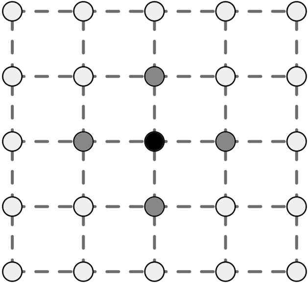
(a)

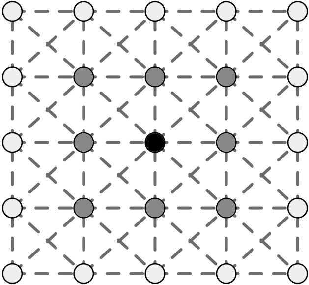
(b)

Figure 1: Neighborhood graphs $\mathscr{G}$ of hidden Potts model. (a) The four closest neighbour graph $\mathscr{G}_{4}$ defining model $\text{HPM}(\mathscr{G}_{4},\theta,K)$. (b) The eight closest neighbour graph $\mathscr{G}_{8}$ defining model $\text{HPM}(\mathscr{G}_{8},\theta,K)$.

We set the emission distribution such that the marginal distribution are Gaussian distribution entered at the value of the related nodes, namely

$$y_{i}\mid x_{i}=k~{}\sim\mathcal{N}\left(k,\sigma_{k}^{2}\right)\quad k\in\{0,\ldots,K-1\},$$

where $\sigma_{k}$ is the standard deviation for sites belonging to class $k$. Even though the noise model is homoscedastic, we still index the standard deviation by $k$ since we do not use the assumption of a constant variance in the estimation procedure, such that the number of parameters estimated is $d_{m}=2\times k+1$. The parameter to be estimated with the ICM or simulated field algorithms is then $\theta=\left(\phi,\psi\right),~{}\text{with}~{}\phi=\left\{\left(k,\sigma_{k}\right):~{}k=0,\ldots,K-1\right\}.$ We denote ${\rm HPM}(\mathscr{G},\theta,K)$, the hidden K-states Potts model defined above.

The common point of our examples is to select the hidden Potts model that better fits a given observation $\mathbf{y}^{\text{obs}}$ composed of $n=100\times 100$ pixels among a collection

$$\mathcal{M}=\left\{{\rm HPM}\left(\mathscr{G},\theta,K\right):~{}K=K_{\rm min},\ldots,K_{\rm max}~{};~{}\mathscr{G}\in\left\{\mathscr{G}_{4},\mathscr{G}_{8}\right\}\right\},$$

where $K$ is the number of colors of the corresponding model and $\mathscr{G}$ is one of the two possible neighborhood systems: $\mathscr{G}_{4}$ and $\mathscr{G}_{8}$, see Figure 1. For each model ${\rm HPM}\left(\mathscr{G},\theta,K\right)$, the estimate $\hat{\theta}_{\text{MLE}}$ and the segmented field $\tilde{\mathbf{x}}$ were computed using $\rm SpaCEM^{3}$ (see the Documentation on http://spacem3.gforge.inria.fr). The software allows the implementation of the unsupervised ICM algorithm as well as the simulated field algorithm and provides computation of PLIC, the mean field-like approximations $\text{BIC}^{\text{MF-like}}$ and $\text{BIC}^{\text{GBF}}$. The ICM and the EM-like algorithms were both initialized with a simple $K$-means procedure. The stopping criterion is then settled to a number of 200 iterations that is enough to ensure the convergence of the procedure.

In what follows, we restrict each $A(\ell)$ to be of the same dimension and in particular square block of dimension $b\times b$. For the sake of clarity the Block Likelihood Criterion is indexed by the dimension of the blocks, namely for a partition of square blocks of size $b\times b$ for which $\tilde{\mathbf{x}}=\tilde{\mathbf{x}}^{\text{MF-like}}$ and $\hat{\theta}_{\text{MLE}}=\hat{\theta}^{\text{MF-like}}$, we note it $\text{BLIC}^{\text{MF-like}}_{b\times b}$. As already mentioned, we then have $\text{BIC}^{\text{MF-like}}=\text{BLIC}_{1\times 1}^{\text{MF-like}}$. We recall that when $B(\ell)=\emptyset$, $\tilde{\mathbf{x}}$ is omitted in the previous notations, that is for a square blocks partition we note our criterion $\text{BLIC}_{b\times b}$. Then $\text{BLIC}_{1\times 1}$ is the BIC approximations corresponding to a finite independent mixture model. All criterion were tested on simulated images obtained using the Swendsen-Wang algorithm. We describe below the different experiments settings we have considered and the results we got.

4.2 First experiment: selection of the number of colors

In this experiment the dependency structure is assumed to be known and the aim is to recover the number $K$ of colors of the latent configuration. We considered realizations from hidden Potts models with $K_{T}=4$ colors and $\sigma_{k}=0.5$. The interaction parameter $\psi$ was set close to the phase transition, namely $\psi=1$ and $\psi=0.4$ for $\mathscr{G}_{4}$ and $\mathscr{G}_{8}$ respectively. These values of the parameter ensure the images present homogeneous regions and then the observations exhibit some spatial structure. Such settings illustrate the advantage of taking into account spatial information of the model. Obviously, for values of $\psi$ where the interaction is weaker, the benefit of the criterion that include the dependency structure of the model is not clear. The latter could even be misleading in comparison with BIC approximations for independent mixture models when $\psi$ is close to zero. On the other side, when $\psi$ is above the phase transition, the distribution on $\mathscr{X}^{n}$ becomes heavily multi-modal and there is almost solely one class represented in the image regardless the number of colors of the model. We carried out 100 simulations from the first order neighborhood structure $\mathscr{G}_{4}$ and 100 simulations from the second order neighborhood structure $\mathscr{G}_{8}$.

Table 1: Selected $K$ in the first experiment for 100 realizations from ${\rm HPM}(\mathscr{G}_{4},\theta,4)$ and 100 realizations from ${\rm HPM}(\mathscr{G}_{8},\theta,4)$ using Pseudolikelihood Information Criterion (PLIC), mean field-like approximations ($\text{BIC}^{\text{MF-like}}$, $\text{BIC}^{\text{GBF}}$) and Block Likelihood Information Criterion (BLIC) for various sizes of blocks and border conditions.

	${\rm HPM}(\mathscr{G}_{4},\theta,4)$
K	2	3	4	5	6	7
PLIC	0	9	91	0	0	0
$\text{BIC}^{\text{MF-like}}$	0	0	39	23	16	22
$\text{BIC}^{\text{GBF}}$	0	0	39	25	18	18
$\text{BLIC}^{\text{MF-like}}_{2\times 2}$	0	0	58	18	8	16
$\text{BLIC}_{1\times 1}$	0	0	97	1	2	0
$\text{BLIC}_{2\times 2}$	0	0	100	0	0	0

	${\rm HPM}(\mathscr{G}_{8},\theta,4)$
K	2	3	4	5	6	7
PLIC	0	7	93	0	0	0
$\text{BIC}^{\text{MF-like}}$	0	0	43	18	19	20
$\text{BIC}^{\text{GBF}}$	0	0	52	20	19	9
$\text{BLIC}^{\text{MF-like}}_{2\times 2}$	0	0	52	14	17	17
$\text{BLIC}_{1\times 1}$	0	3	90	1	4	2
$\text{BLIC}_{2\times 2}$	0	1	99	0	0	0
$\text{BLIC}_{4\times 4}$	0	0	100	0	0	0

The results obtained for the different criterion are reported in Table 1. For $b\geq 2$, $\text{BLIC}_{b\times b}$ outperform the different criterion even though PLIC and $\text{BLIC}_{1\times 1}$ provide good results. By contrast approximations based on mean field-like approximations, that is $\text{BIC}^{\text{MF-like}}$, $\text{BIC}^{\text{GBF}}$ and $\text{BLIC}_{2\times 2}^{\text{MF-like}}$, perform poorly. These conclusions need nonetheless to be put into perspective. Figure 2(a) shows that the main issue encountered by these criterion is their inability to discriminate between the more complex models. Indeed these BIC approximations reach a plateau from $K=4$, a problem that other criterion do not face. As an example, Figure 2(b) and Figure 2(c) represent boxplots of the difference between BIC values for ${\rm HPM}(\mathscr{G}_{4},\theta,K)$ as $K$ is increasing for the 100 realizations, namely

$$\Delta\left(K\rightarrow K+1\right)=\text{BIC}\left({\rm HPM}(\mathscr{G},\hat{\theta}_{\text{MLE}},K+1)\right)-\text{BIC}\left({\rm HPM}(\mathscr{G},\hat{\theta}_{\text{MLE}},K)\right),$$

for $K=K_{\rm min},\ldots,K_{\rm max}$. Hence, BIC approximations grow with $K$ if $\Delta\left(K\rightarrow K+1\right)\geq 0$ and decrease otherwise. It appears that $\text{BLIC}_{2\times 2}$ increases systematically from $K=4$ whereas $\text{BIC}^{\text{MF-like}}$ tend to be constant, or even decreases, so that none minimum can be clearly identified. We do not provide the boxplots for $\text{BIC}^{\text{MF-like}}$ and $\text{BIC}^{\text{GBF}}$ because they are significantly the same.

Finally these results illustrate in particular the importance of a well chosen segmented field $\tilde{\mathbf{x}}$. Indeed PLIC and $\text{BIC}^{\text{MF-like}}$ are both criterion of type $\text{BLIC}_{1\times 1}^{\tilde{\mathbf{x}}}$ but their performances greatly differ on this example. As regards the selection of $K$, $\text{BLIC}_{b\times b}$ circumvent this question whilst performing better.

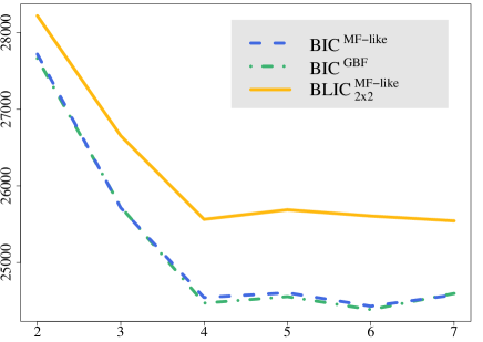
(a)

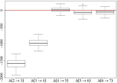
(b)

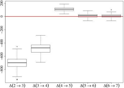
(c)

Figure 2: First experiment results. (a) $\text{BIC}^{\text{MF-like}}$, $\text{BIC}^{\text{GBF}}$ and $\text{BLIC}_{2\times 2}^{\text{MF-like}}$ values for one realization of a first order hidden Potts model ${\rm HPM(\mathscr{G},\theta,4)}$. (b) Difference between $\text{BLIC}^{\text{MF-like}}_{2\times 2}$ values for 100 realization of a first order hidden Potts model ${\rm HPM}(\mathscr{G}_{4},\theta,4)$ as $K$ is increasing. (c) Difference between $\text{BLIC}_{2\times 2}$ values for 100 realization of a first order hidden Potts model ${\rm HPM}(\mathscr{G}_{4},\theta,4)$ as $K$ is increasing

4.3 Second experiment: selection of the dependency structure

For this second experiments the setting was exactly the same than for the first experiment. The only difference is that as first instance the number of colors $K_{T}$ is assumed to be known while the neighborhood system has to be chosen. To answer such a question it is obvious that we can not use criterion $\text{BLIC}_{1\times 1}$ based on independent mixture model.

As regards this question, all but two criterion perform very well, see Table 2. In the first place, PLIC faces trouble to select the correct $\mathscr{G}_{4}$. This illustrate the importance of the estimation of the interaction parameter $\psi$. We have observed that the ICM algorithm whilst providing good segmented field, produces poorer estimates of the parameter than the simulated field algorithm. This has an impact quite important since $\psi$ sets the strength of interaction between neighboring nodes of the graph $\mathscr{G}$ and is most representative of the spatial correlation. On the other hand, $\text{BLIC}_{2\times 2}$ fails to select the neighborhood system for second order hidden Potts model ${\rm HPM}(\mathscr{G}_{8},\theta,4)$. This conclusion can be simply explained by the fact that the block does not include enough spatial information to discriminate between the competing models. When the primary purpose is the selection of a dependency structure, we should use block large enough to be informative regarding the different neighborhood systems in competition.

H ${\rm HPM}(\mathscr{G}_{4},\theta,4)$ $\mathscr{G}_{4}$ $\mathscr{G}_{8}$ PLIC 53 47 $\text{BIC}^{\text{MF-like}}$ 100 0 $\text{BIC}^{\text{GBF}}$ 100 0 $\text{BLIC}^{\text{MF-like}}_{2\times 2}$ 100 0 $\text{BLIC}_{2\times 2}$ 100 0 ${\rm HPM}(\mathscr{G}_{8},\theta,4)$ $\mathscr{G}_{4}$ $\mathscr{G}_{8}$ PLIC 0 100 $\text{BIC}^{\text{MF-like}}$ 0 100 $\text{BIC}^{\text{GBF}}$ 0 100 $\text{BLIC}^{\text{MF-like}}_{2\times 2}$ 0 100 $\text{BLIC}_{2\times 2}$ 59 41 $\text{BLIC}_{4\times 4}$ 0 100

Table 2: Selected $\mathscr{G}$ in the second experiment for 100 realizations from ${\rm HPM}(\mathscr{G}_{4},\theta,4)$ and 100 realizations from ${\rm HPM}(\mathscr{G}_{8},\theta,4)$ using Pseudolikelihood Information Criterion (PLIC), mean field-like approximations ($\text{BIC}^{\text{MF-like}}$, $\text{BIC}^{\text{GBF}}$) and Block Likelihood Information Criterion (BLIC) for various sizes of blocks and border conditions.

Aside the two above exceptions, the good performances of all criteria can be surprising. The same experiment has been done for stronger noise with $\sigma_{k}=0.75$ and $\sigma_{k}=1$. The conclusion remains the same. It appears that for a conditionally independent noise process, neighborhood system are readily distinguished close to the phase transition. This is not true for any parameter value as illustrated in the third experiment.

In the second instance, we supposed that $K_{T}$ and $\mathscr{G}$ were unknown, so that we were interested in the joint selection of the number of colors and of the dependency graph. For this example, the results remain the same than in Table 1 with the exception of PLIC. Indeed, the different criterion manage to differentiate the model in terms of the graph $\mathscr{G}$ so that their performances are directly related to their ability to choose the correct number of colors.

4.4 Third experiment: BLIC versus ABC

This third experiment is the occasion to compare BLIC with the ABC procedures proposed by Stoehr et al., (2015). We return to the problem of solely selecting the dependency graph when the number of colors is known. We still consider a homoscedastic Gaussian noise but over bicolor Potts models (K=2). The standard deviation $\sigma_{k}=0.39$, $k\in\{0,1\}$, was set so that the probability of a wrong prediction of the latent color with a marginal MAP rule on the Gaussian model is about $10\%$ in the thresholding step of the ABC procedure. Regarding the dependency parameter $\psi$, we set prior distributions below the phase transition which occurs at different levels depending on the neighborhood structure. Precisely we used a uniform distribution over $(0;1)$ when the adjacency is given by $\mathscr{G}_{4}$ and a uniform distribution over $(0;0.35)$ with $\mathscr{G}_{8}$. In order to examine the performance of model choice criteria in comparison of ABC, we carried out 1000 realizations from ${\rm HPM}(\mathscr{G}_{4},\theta,2)$ and 1000 realizations from ${\rm HPM}(\mathscr{G}_{8},\theta,2)$ with parameters from the priors. The results are presented in Table 3

H Train size $\bf 5,000$ $\bf 100,000$ Criterion Error rate 2D statistics $14.2\%$ $13.8\%$ PLIC $19.8\%$ 4D statistics $10.8\%$ $9.8\%$ $\text{BIC}^{\text{MF-like}}$ $7.6\%$ 6D statistics $8.6\%$ $6.9\%$ $\text{BIC}^{\text{GBF}}$ $7.1\%$ Adaptive ABC $8.2\%$ $6.7\%$ $\text{BLIC}_{4\times 4}$ $7.7\%$

Table 3: Evaluation of the prior error rate of ABC procedures and of the error rate for the model choice criterion in the third experiment.

The novel ABC procedure introduced by Stoehr et al., (2015) appears to provide the best performances but for a training reference table of size 100 000. This reinforces the idea that for unlimited computation possibilities, ABC can efficiently address situations where the likelihood is intractable. However, Table 3 suggest that for a much lower computational cost it is possible to get equivalent, or even better, error rate by using model choice criterion $\text{BIC}^{\text{MF-like}}$, $\text{BIC}^{\text{GBF}}$ or $\text{BLIC}_{b\times b}$, while PLIC seems not to be overtaken. In this example, $\text{BIC}^{\text{GBF}}$ slightly supersede $\text{BIC}^{\text{MF-like}}$ and $\text{BLIC}_{b\times b}$. This can be explained by the fact that for parameter from the prior close to zero, the assumption of independence between the sites is almost true. In the latter case, estimating BIC using the first order approximations of the partition function of Gibbs distribution (Forbes and Peyrard,, 2003) may be preferable than using normalizing constants defined on blocks.

5 Conclusion and perspective

In the present article, we considered BIC to perform model selection when dealing with hidden Markov random fields. To avoid time consuming simulation methods like MCMC or ABC algorithms, we proposed to move towards variational methods and in particular to use valid probability distributions over non-overlapping blocks of the lattice in place of the intractable likelihood (Section 3.2). Consequently, we derived Block Likelihood Information Criterion to discriminate between hidden Markov random fields.

The numerical results (Section 4) highlighted that the approximations of BIC based on independent blocks without fixed border provide better performances comparing to pre-existing criteria as regards the inference of the number of latent colors. This conclusion has to be brought into perspective for the selection of the dependency structure as the size of the blocks should be wide enough unless BLIC can be misleading. According to the numerical results (Section 4.4), the opportunity we have explored appears to be a satisfactory alternative to ABC model choice algorithms which besides their computational cost are delicate to calibrate (e.g., Stoehr et al.,, 2015). Our approach offers thus an appealing trade-off between efficient computation and reliable results.

While the numerical part of the paper assess its efficiency, the novel criterion makes in its current version two major approximations that are worth exploring. First mention, the choice of a particular substitute is lead by any optimality conditions. From that viewpoint, the construction of an optimal approximations regarding the variational free energy over the set of probability distributions that factorize on blocks is yet to be studied. The second level of approximations concerns the penalty term. The next step of our work cannot be reduced to the sole aim of improving the quality of the approximations. Through Section 4.2, we have seen that an optimal solution with respect to the Kullback- Leibler divergence is not sufficient to ensure a good behaviour of model choice criteria, especially if the more complex model are not enough penalized. The penalty term used is solely valid for independent variable. We have neglected the interaction within a block, an assumption that slightly modified the number of free parameter. The impact of dependence variables on the penalty term is a logical follow-up to our work.

References

- Alfò et al., (2008) Alfò, M., Nieddu, L., and Vicari, D. (2008). A finite mixture model for image segmentation. Statistics and Computing, 18(2):137–150.
- Besag, (1974) Besag, J. E. (1974). Spatial Interaction and the Statistical Analysis of Lattice Systems (with Discussion). Journal of the Royal Statistical Society. Series B (Methodological), 36(2):192–236.
- Besag, (1975) Besag, J. E. (1975). Statistical Analysis of Non-Lattice Data. The Statistician, 24:179–195.
- Besag, (1986) Besag, J. E. (1986). On the Statistical Analysis of Dirty Pictures. Journal of the Royal Statistical Society. Series B (Methodological), 48(3):259–302.
- Besag et al., (1991) Besag, J. E., York, J., and Mollié, A. (1991). Bayesian image restoration, with two applications in spatial statistics. Annals of the institute of statistical mathematics, 43(1):1–20.
- Celeux et al., (2003) Celeux, G., Forbes, F., and Peyrard, N. (2003). EM procedures using mean field-like approximations for Markov model-based image segmentation. Pattern Recognition, 36(1):131–144.
- Clifford, (1990) Clifford, P. (1990). Markov random fields in statistics. Disorder in physical systems: A volume in honour of John M. Hammersley, pages 19–32.
- Csiszár et al., (2000) Csiszár, I., Shields, P. C., et al. (2000). The consistency of the BIC Markov order estimator. The Annals of Statistics, 28(6):1601–1619.
- Csiszár and Talata, (2006) Csiszár, I. and Talata, Z. (2006). Consistent Estimation of the Basic Neighborhood of Markov Random Fields. The Annals of Statistics, 34(1):123–145.
- Cucala and Marin, (2013) Cucala, L. and Marin, J.-M. (2013). Bayesian Inference on a Mixture Model With Spatial Dependence. Journal of Computational and Graphical Statistics, 22(3):584–597.
- Everitt, (2012) Everitt, R. G. (2012). Bayesian Parameter Estimation for Latent Markov Random Fields and Social Networks. Journal of Computational and Graphical Statistics, 21(4):940–960.
- Forbes and Peyrard, (2003) Forbes, F. and Peyrard, N. (2003). Hidden Markov random field model selection criteria based on mean field-like approximations. Pattern Analysis and Machine Intelligence, IEEE Transactions on, 25(9):1089–1101.
- François et al., (2006) François, O., Ancelet, S., and Guillot, G. (2006). Bayesian Clustering Using Hidden Markov Random Fields in Spatial Population Genetics. Genetics, 174(2):805–816.
- Friel, (2012) Friel, N. (2012). Bayesian Inference for Gibbs Random Fields Using Composite Likelihoods. In Proceedings of the Winter Simulation Conference, number 28 in WSC ’12, pages 1–8. Winter Simulation Conference.
- Friel, (2013) Friel, N. (2013). Evidence and Bayes Factor Estimation for Gibbs Random Fields. Journal of Computational and Graphical Statistics, 22(3):518–532.
- Friel et al., (2009) Friel, N., Pettitt, A. N., Reeves, R., and Wit, E. (2009). Bayesian Inference in Hidden Markov Random Fields for Binary Data Defined on Large Lattices. Journal of Computational and Graphical Statistics, 18(2):243–261.
- Friel and Rue, (2007) Friel, N. and Rue, H. (2007). Recursive computing and simulation-free inference for general factorizable models. Biometrika, 94(3):661–672.
- Gassiat, (2002) Gassiat, E. (2002). Likelihood ratio inequalities with applications to various mixtures. Annales de l’Institut Henri Poincare (B) Probability and Statistics, 38(6):897–906.
- Geman and Geman, (1984) Geman, S. and Geman, D. (1984). Stochastic Relaxation, Gibbs Distributions, and the Bayesian Restoration of Images. IEEE Transactions on Pattern Analysis and Machine Intelligence, 6(6):721–741.
- Green and Richardson, (2002) Green, P. J. and Richardson, S. (2002). Hidden Markov Models and Disease Mapping. Journal of the American Statistical Association, 97(460):1055–1070.
- Grelaud et al., (2009) Grelaud, A., Robert, C. P., Marin, J.-M., Rodolphe, F., and Taly, J.-F. (2009). ABC likelihood-free methods for model choice in Gibbs random fields. Bayesian Analysis, 4(2):317–336.
- Grimmett, (1973) Grimmett, G. R. (1973). A theorem about random fields. Bulletin of the London Mathematical Society, 5(1):81–84.
- Haughton, (1988) Haughton, D. M. A. (1988). On the Choice of a Model to Fit Data from an Exponential Family. The Annals of Statistics, 16(1):342–355.
- Hurn et al., (2003) Hurn, M. A., Husby, O. K., and Rue, H. (2003). A Tutorial on Image Analysis. In Spatial Statistics and Computational Methods, volume 173 of Lecture Notes in Statistics, pages 87–141. Springer New York.
- Ji and Seymour, (1996) Ji, C. and Seymour, L. (1996). A consistent model selection procedure for Markov random fields based on penalized pseudolikelihood. The annals of applied probability, pages 423–443.
- Jordan et al., (1999) Jordan, M. I., Ghahramani, Z., Jaakkola, T. S., and Saul, L. K. (1999). An Introduction to Variational Methods for Graphical Models. Machine learning, 37(2):183–233.
- Kass and Raftery, (1995) Kass, R. E. and Raftery, A. E. (1995). Bayes factors. Journal of the american statistical association, 90(430):773–795.
- Kass and Wasserman, (1995) Kass, R. E. and Wasserman, L. (1995). A reference Bayesian test for nested hypotheses and its relationship to the schwarz criterion. Journal of the American Statistical Association, 90(431):928–934.
- Keribin, (2000) Keribin, C. (2000). Consistent Estimation of the Order of Mixture Models. Sankhy: The Indian Journal of Statistics, Series A (1961-2002), 62(1):49–66.
- Lindsay, (1988) Lindsay, B. G. (1988). Composite likelihood methods. Contemporary Mathematics, 80(1):221–39.
- Marin et al., (2012) Marin, J.-M., Pudlo, P., Robert, C. P., and Ryder, R. J. (2012). Approximate Bayesian Computational methods. Statistics and Computing, 22(6):1167–1180.
- McGrory et al., (2009) McGrory, C. A., Titterington, D. M., Reeves, R., and Pettitt, A. N. (2009). Variational Bayes for estimating the parameters of a hidden Potts model. Statistics and Computing, 19(3):329–340.
- Moores et al., (2014) Moores, M. T., Hargrave, C. E., Harden, F., and Mengersen, K. (2014). Segmentation of cone-beam CT using a hidden Markov random field with informative priors. Journal of Physics : Conference Series, 489.
- Okabayashi et al., (2011) Okabayashi, S., Johnson, L., and Geyer, C. J. (2011). Extending pseudo-likelihood for Potts models. Statistica Sinica, 21(1):331.
- Qian and Titterington, (1991) Qian, W. and Titterington, D. (1991). Estimation of parameters in hidden Markov models. Philosophical Transactions of the Royal Society of London. Series A: Physical and Engineering Sciences, 337(1647):407–428.
- Raftery, (1995) Raftery, A. E. (1995). Bayesian model selection in social research. Sociological methodology, 25:111–164.
- Reeves and Pettitt, (2004) Reeves, R. and Pettitt, A. N. (2004). Efficient recursions for general factorisable models. Biometrika, 91(3):751–757.
- Schwarz, (1978) Schwarz, G. (1978). Estimating the dimension of a model. The annals of statistics, 6(2):461–464.
- Seymour and Ji, (1996) Seymour, L. and Ji, C. (1996). Approximate Bayes model selection procedures for Gibbs-Markov random fields. Journal of Statistical Planning and Inference, 51(1):75–97.
- Stanford and Raftery, (2002) Stanford, D. C. and Raftery, A. E. (2002). Approximate Bayes factors for image segmentation: The pseudolikelihood information criterion (PLIC). Pattern Analysis and Machine Intelligence, IEEE Transactions on, 24(11):1517–1520.
- Stoehr and Friel, (2015) Stoehr, J. and Friel, N. (2015). Calibration of conditional composite likelihood for bayesian inference on gibbs random fields. In JMLR WCP: Proceedings of the Eighteenth International Conference on Artificial Intelligence and Statistics, volume 38, pages 921–929.
- Stoehr et al., (2015) Stoehr, J., Pudlo, P., and Cucala, L. (2015). Adaptive ABC model choice and geometric summary statistics for hidden Gibbs random fields. Statistics and Computing, 25(1):129–141.
- Tierney and Kadane, (1986) Tierney, L. and Kadane, J. B. (1986). Accurate Approximations for Posterior Moments and Marginal Densities. Journal of the American Statistical Association, 81(393):82–86.