Capture into resonance and phase space dynamics in optical centrifuge

Abstract

The process of capture of a molecular enesemble into rotational resonance in the optical centrifuge is investigated. The adiabaticity and phase space incompressibility are used to find the resonant capture probability in terms of two dimensionless parameters $P_{1,2}$ characterising the driving strength and the nonlinearity, and related to three characteristic time scales in the problem. The analysis is based on the transformation to action-angle variables and the single resonance approximation, yielding reduction of the three-dimensional rotation problem to one degree of freedom. The analytic results for capture probability are in a good agreement with simulations. The existing experiments satisfy the validity conditions of the theory.

I Introduction

The field of optical control and manipulation of molecular rotation has seen major advances over the years, and today various techniques allow to control the rotation alignment alignment1 ; alignment2 , orientation orientation1 ; orientation2 and directionality rotation1 ; rotation2 ; rotation3 of molecular ensembles. One of the most innovative tools in this field is the optical centrifuge (OC), originally proposed and implemented by Corkum and collaborators Corkum1 ; Corkum2 , who introduced the possibility of controlled excitation of the molecular rotational degree of freedom by chirped laser pulses. The controlled nature of this process is twofold: the molecules reach very high rotational states (super rotors), but they also remain closely centered around a specific target energy/frequency. The controlled rotation could be used to selectively dissociate molecules Corkum2 or a specific molecular bond HCNbreaking and has been shown to change molecular characteristics, such as the molecule’s stability against collisions Forrey and its scattering from surfaces averbukh1 . Furthermore, a gas of super rotors may exhibit new optical properties averbukh2 and formation of vortices averbukh3 .

Over the last few years, several state of the art experiments have been performed mullin1 ; milner1 ; milner2 utilizing different molecules, and exploring the dynamics during and after the OC laser pulse, including the excitation process milner1 , the gyroscopic stage in which the molecules remain oriented milner3 and the equilibration and thermalization that follows the pulse and produces an audible sound wave milner4 . However, while the experimental setups improved considerably, the process of capture of molecules into the chirped resonant rotation is still poorly understood. This process was only studied numerically ivanov1 or under the constraint that the molecules rotate in a plane perpendicular to the laser propagation axis Corkum1 ; ivanov2 ; girard . The former asumption makes it impossible to study the response of a randomly oriented molecular ensemble to the OC pulse. As a result, the efficiency of the OC, i.e. the fraction of molecules captured by the chirped laser drive, was not analyzed sufficiently.

In this work, we will show that under the rigid-rotor approximation the OC is an example within a broad family of driven non-linear systems exhibiting a sustained phase-locking or autoresonance (AR) with a chirped drive. This phenomenon has been observed and studied in many applications, including atomic systems AR1 ; AR2 , plasmas AR3 ; AR4 , fluids AR5 , and semiconductor quantum wells AR6 . By using methods in the theory of AR and analyzing the associated phase space dynamics we will for the first time calculate the efficiency of the OC process. The quantum counterpart of the AR is the quantum energy ladder climbing AR6a ; AR7 ; AR8 , but we will show that the classical AR analysis is relevant to many current experimental setups.

The scope of the paper will be as follows. In Sec. II, we will discuss the driven-chirped molecular rotation in three dimensions, transform to action-angle variables, and use the single resonance approximation to reduce the problem to one degree of freedom. Section III will focus on calculating the efficiency of the resonant capture process in the system via analysing its dynamics in a continuous phase space instead of a single particle approach. In section IV, we will compare the theory with numerical simulations and discuss the validity of our approximations and the applicability to current experimental setups. Our conclusions will be summarized in Sec. V.

II The model

II.1 Parameterization

The fundamental idea of the OC, is that an anisotropic molecule will ”chase” (and, thus, be rotationally excited) a rotating linearly polarized wave, whose polarization rotation accelerates over time. In practice, such driving wave is created by combining two counter rotating and antichirped circularly polarized laser beams Corkum1 . For a wave propagating along the $Z$ axis, with polarization angle $\phi_{d}\left(t\right)$ in the $XY$ plane, after averaging over the optical frequency of the laser beams, the interaction potential energy of a molecule in spherical coordinates is given by $U=-\varepsilon\sin^{2}\theta\cos^{2}\left(\varphi-\phi_{d}\right)$ Corkum1 , where $\varepsilon=\left(\alpha_{\parallel}-\alpha_{\perp}\right)E_{0}^{2}/4$, $\alpha_{\parallel}$,$\alpha_{\perp}$ are the polarizability components of the molecule and $E_{0}$ is the electric field amplitude of the combined beam. For simplicity, we will use a linearly chirped driving frequency $\omega_{d}=d\phi_{d}/dt=\beta t/2$, where $\beta>0$ is the chirp rate, but any sufficiently slow chirp will lead to similar results. The initial rotation frequency is set by taking an appropriate intial time.

Our driven system can be characterized by three different time scales, i.e. the drive sweeping time $t_{s}=1/\sqrt{\beta}$, the characteristic thermal rotation time $t_{th}=1/\omega_{th}=\sqrt{I/k_{B}T}$, and the driving time scale $t_{d}=L_{th}/\varepsilon=\sqrt{Ik_{B}T}/\varepsilon$, where $T$ is the temperature, $I$ the molecule’s moment of inertia, and $L_{th}=I\omega_{th}$ is the characteristic thermal angular momentum. These three time scales define two dimensionless parameters,

$$P_{1}=\frac{t_{s}}{t_{d}}=\frac{\varepsilon}{\sqrt{Ik_{B}T\beta}},$$ (1)

which measures the drive’s strength, and

$$P_{2}=\frac{t_{s}}{t_{th}}=\sqrt{\frac{k_{B}T}{I\beta}},$$ (2)

characterizing the nonlinearity of the problem. These parameters enter naturally in the dimensionless Hamiltonian of our driven system in spherical coordinates

$$H=\frac{P_{2}}{2}\left(p_{\theta}^{2}+\frac{p_{\varphi}^{2}}{\sin^{2}{\theta}}\right)-P_{1}\sin^{2}\theta\cos^{2}\left(\varphi-\phi_{d}\right),$$ (3)

where we normalize the canonical momenta and later the total angular momentum $L$ with respect to $L_{th}$, and use the dimensionless time $\tau=\sqrt{\beta}t$.

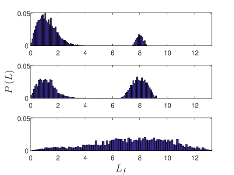
Figure 1: Monte Carlo simulation of the distribution of angular momenta $L_{f}$ for initially thermal ensemble (3000 molecules) after the OC pulse with initial and final normalized driving frequencies $\omega_{0}=1$ and $\omega_{f}=8$. The oarameters are $P_{2}=2.51$ and $P_{1}=0.63,2.51,39.8$ in pannels (a)-(c), respectively

The evolution equations based on this Hamiltonian comprised one of the two sets used for Monte Carlo simulations in this work. Figure 1 shows the distributions (histograms) of the normalized angular momenta at the end of the chirped OC drive after starting from initially thermal molecular ensemble. The resonant normalized angular momentum in the OC equals the instantaneous driving frequency normalized with respect to $\omega_{th}$ (see below). The initial and final normalized driving frequencies in Fig. 1 were $1$ and $8$, respectively, and we used parameters $P_{2}=2.51$ and $P_{1}=0.63$ (Fig. 1a), $2.51$ (Fig. 1b), $39.8$ (Fig. 1c). When parameter $P_{1}$ is increased (for constant $P_{2}$ this corresponds to increasing the laser intensity), more molecules experience significant acceleration. Nevertheless, if one seeks a narrow distribution around a specific target frequency, the acceleration in panels (b) and (c) Fig. 1 does not provide the desired level of control, showing a broad distribution around the target. In contrast, panel (a), is a representative example for the degree of control and accuracy one can achieve with the OC, provided the parameters are chosen appropriatly. In this work we calculate the excitation efficiency and the width of the final distribution of the angular momentum in the $P_{1,2}$ parameter space.

II.2 Transformation to action-angle variables and single-resonance approximation

Like in many other physical systems, it is convenient to transform our driven problem to the action-angle variables of the unperturbed problem since the latter is integrable. This canonical transformation $\theta,\varphi,p_{\theta},p_{\varphi}\rightarrow\Theta_{L},\Theta_{L_{z}},L,L_{z}$ (see Appendix A for details) leads to non trivial angle variables (related to Euler angles), while the actions $L$ and $L_{z}$ are the normalized total angular momentum and its projection on the $Z$ axis. The transformed Hamiltonian assumes the form:

$$H\left(\Theta_{L},\Theta_{L_{z}},L,L_{z}\right)=P_{2}\frac{L^{2}}{2}+P_{1}U\left(\Theta_{L},\Theta_{L_{z}},L_{z}/L,\phi_{d}\right),$$ (4)

where $U$ is a periodic function of $\Theta_{L},\Theta_{L_{z}}$ of period $\pi$, and its exact form is presented in the appendix.

The perturbing part in (4) contains several oscillating terms, however, the main resonance in our case is defined by requiring stationarity $\Phi\approx const$ of the phase-mismatch $\Phi=2(\Theta_{L}+\Theta_{L_{z}}-\phi_{d})$. Assuming a weak drive, i.e. $P_{1}/P_{2}\ll 1$ (this approximation will be discussed in Sec. IV) in the vicinity of the resonance, we can use the single resonance approximation chirikov , i.e. discard all the rapidly oscillating terms in the Hamiltonian. The resulting approximate, single resonance Hamiltonian is (see Appendix A):

$$H_{r}=P_{2}\frac{L^{2}}{2}+P_{1}V\cos{\Phi}+P_{1}F,$$ (5)

where

$$V = \frac{1}{8}\left(1+\frac{L_{z}}{L}\right)^{2},$$ (6)

$$F = \frac{1}{4}\left(1-\frac{{L_{z}}^{2}}{L^{2}}\right).$$ (7)

The corresponding evolution equations are

$$\frac{d\Theta_{L}}{d\tau} = P_{2}L-P_{1}\frac{L_{z}}{L^{2}}\left(V^{\prime}\cos{\Phi}+F^{\prime}\right),$$ (8)

$$\frac{d\Theta_{L_{z}}}{d\tau} = P_{1}\frac{1}{L}\left(V^{\prime}\cos{\Phi}+F^{\prime}\right),$$ (9)

$$\frac{dL}{d\tau} = 2P_{1}V\sin{\Phi},$$ (10)

$$\frac{dL_{z}}{d\tau} = 2P_{1}V\sin{\Phi}.$$ (11)

Here, the prime denotes differentiation with respect to $L_{z}/L$. Equations (10), (11) yield the integral of motion $C=L-L_{z}$ ($0\leq C\leq 2L$), which allows reduction to a single degree of freedom:

$$\frac{dL}{d\tau} = 2P_{1}V\sin{\Phi},$$ (12)

$$\frac{d\Phi}{d\tau} = 2P_{2}L+2P_{1}\frac{C}{L^{2}}\left(V^{\prime}\cos{\Phi}+F^{\prime}\right)-\tau.$$ (13)

Equation (9) still needs to be solved to obtain the precession of the angular momentum around the $Z$-axis, but for calculating $L,$ the one degree of freedom set above is sufficient. This is our second (approximate) set used in the simulations below, which, due to the adiabaticity and reduced number of degrees of freedom, is considerably faster numerically than the full set of evolution equations in terms of the original spherical coordinates. We will assume, and verify a posteriori that if $\Delta L\ll 1$ is the range of $L$ values in a persistent resonance with the drive in our problem, then $P_{2}\Delta L\gg P_{1}$. Under this assumption, the second term in Eq. (13) can be neglected, and the phase locking (resonance) condition $d\Phi/d\tau\approx 0$ yields $2P_{2}L-\tau\approx 0$. Let $L_{r}(\tau)=\tau/2P_{2}=\omega_{d}(\tau)/\omega_{th\text{ }}$be the value of $L$ satisfying the resonance condition exactly and define the deviation $\delta L=L-L_{r}$ from the exact resonance. The evolution equations then yield

$$\frac{d\delta L}{d\tau} = 2P_{1}V\sin{\Phi}-\frac{1}{2P_{2}},$$ (14)

$$\frac{d\Phi}{d\tau} = 2P_{2}\delta L.$$ (15)

By taking the derivative of Eq. (15) with respect to time and inserting Eq. (14), we get

$$\frac{d^{2}\Phi}{d\tau^{2}}=-4P_{1}P_{2}V\sin{\Phi}-1,$$ (16)

where we shifted $\Phi$ by $\pi$ and, to lowest order in $\delta L$, $V\approx\frac{1}{8}\left(2-\frac{C}{L_{r}}\right)^{2}$ is evaluated at $L_{r}$. Equation (16) describes a pseudo-pendulum under the action of a constant torque. The Hamiltonian in this problem, with $d\Phi/d\tau$ acting as the momentum, is:

$$H=\frac{1}{2}\left(\frac{d\Phi}{d\tau}\right)^{2}+V_{eff}\left(\Phi\right),$$ (17)

where

$$V_{eff}\left(\Phi\right)=-4P_{1}P_{2}V\cos{\Phi}+\Phi.$$ (18)

This tilted cosine effective potential and the associated phase space portrait of dynamics of the pseudo-pendulum are shown in Fig. 2 for $P_{1}P_{2}V=0.75$. The phase space (bottom panel in the figure) is comprised of open and closed trajectories, provided $P_{1}P_{2}V>1/4$. The open trajectories exhibit a continuous growth of the phase-mismatch, i.e. are not phase locked with the drive, while for the closed trajectories the phase-mismatch is bounded. The closed trajectories are surounded by the separatrix having area shown in red in the bottom panel of the figure. As $V(L_{r})$ in our problem is slowly varying (increasing) in time, both the closed and open trajectories evolve adiabatically in time, unless near the separatrix. This means that deeply trapped trjectories remain trapped, i.e the rotation frequency follows the drive, $L(\tau)\approx\omega_{d}(\tau)/\omega_{th\text{ }}$, constituting the AR in the system. The main problem remains the fate of the trajectories near the separatrix. These trajectories, in principle, can change their trapping status as the result of nonadiabatic dynamics and, thus,  affect the OC efficiency. It should be mentioned that many other AR systems AR3 ; AR4 ; AR5 ; AR6 are described by the resonant Hamiltonian similar to (17). The process of capture into resonance in all these problems depends critically on the specific form of function $V$. In many such problems $V\sim\sqrt{I}$, where $I$ is the relevant action variable in the problem. In all such cases, the capture into resonance from equilibrium and transition to AR is guaranteed provided the driving amplitude exceeds a sharp threshold AR3 . Because of a different dependence of $V$ on $L$ no such threshold is characteristic of the driven molecule case. The study of this different capture mechanism comprises the main goal of the present investigation.

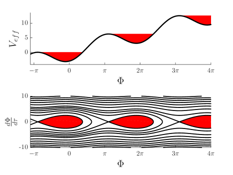
Figure 2: The effective potential (Eq. 18) (top panel) and the phase-space portrait of the associated dynamics (bottom panel). The boundary of the red filled area in the bottom panel is the separatrix. The value of $P_{1}P_{2}V$ was $0.75$ and the equal energy lines in the bottom panel are separated by energy steps of $\pi$.

III
Trapping Efficiency

III.1 The complexity of resonant trapping problem

We have seen in simulations in Sec. II that for a range of parameters, the OC yields controlled rotational excitation of molecular ensembles. Here we study the efficiency of such excitation process, i.e. evaluate the fraction of molecules from some initial distribution, which are captured into and remain in resonance. Intuitively, one can assume that if the value of $V$ changes adiabatically, molecules will be either trapped or not according to their initial location in phase space - inside or outside the separatrix. While the changes of $V$ are generally adiabatic (as will be seen later), this intuition proves to be wrong. Indeed, the molecules which are inside the separatrix initially remain in resonance at later times, but additional molecules can cross the separatrix and enter the trapped region even if they were outside initially. An illustration of this process is presented in Fig. 3, where panel (a) shows the final phase-space distribution of a molecular ensemble having the same $L=1$ and $C=1$ initially and uniformly distributed values of $\Phi$ (see panel b). The normalized driving frequency was varied from $\omega_{0}=0.5$ to $\omega_{f}=1.5$, and one can see that despite a much lower initial driving frequency compared to the rotation frequency of the molecules, a considerable amount of molecules end up captured into resonance and rotationally accelerated (green). The location of the newly trapped molecules in the initial ensemble is shown in green in panel (b). We find that this location and the fraction of trapped molecules strongly depends on the initial value of the driving frequency. This complexity is illustrated in panels (c) and (d), showing in green the location of the molecules trapped in resonance with the drive for the same initial conditions, but with the initial driving frequency changed by $\pm 0.01$. The fraction of the trapped molecules in cases (c) and (d) was $22\%$ and $26\%$, respectively compared to $46\%$ in the case (a-b).

One approach to deal with the nonadiabatic passage through separatrix problem is to study an ensemble of initial conditions, checking whether the associated trajectories cross the separatrix. Previous works used such approach with simpler systems, but the probabilistic nature of this nonadiabatic phenomenon led to rather complex results dioctorn ; neishtadt . Here, we will develop an alternative approach which examines the continuous phase space dynamics of the initial ensemble, instead of working with a collection of individual trajectories. This approach will yield the resonant capture probability, without ever specifying which initial conditions yield trajectories crossing the separatrix.

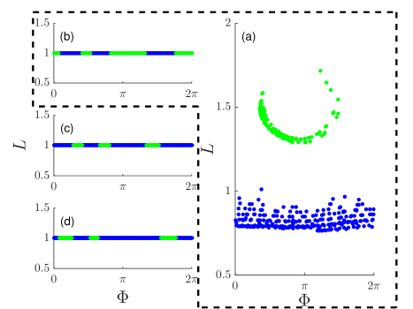
Figure 3: (Color online) Numerical simulations (single resonance approximation) of passage through resonance with 500 molecules with initial $L_{0}=1$ and $C=1$. All panels show the phase-space ($\Phi$,$L$), with green and blue circles representing resonantly trapped and untrapped molecules, respectively. The left panels show the initial distributions and differ by a small shift of the initial driving frequency: $\omega_{0}=0.5$ (b), $0.49$ (c) and $0.51$ (d). The right panel (a) shows the final distribution of the initial condition (b) at $\omega_{f}=1.5$. The parameters are $P_{1}=1$, $P_{2}=10$ and $\Phi$ is shifted so that $\Phi=0$ is at the saddle point (see subsection III.2).

III.2 Phase-space dynamics

We base our analysis on Eq. (16), where $V=\frac{1}{8}\left(2-\frac{C}{L}\right)^{2}$ is evaluated at $L_{r}$ and, therefore, both $V$ and the associated separatrix area are monotonically increasing functions of time. For molecules close to the separatrix, trapped or untrapped, this approximation is satisfied because $\Delta L\ll 1$, where now we associate $\Delta L$ with the width of the separatrix in $L$. For untrapped molecules far from the separatrix we can still evaluate $V$ at $L_{r}$, because the phase mismatch $\Phi$ for such molecules varies rapidely and the effect of the driving term in the quasipotential averages out. Next, instead of passage through resonance with an ensemble of molecules having the same value of $L$ as illustrated in Fig. 3, we consider an ensemble of molecules with initially uniform density in phase space between $L_{1}=3.5$ and $L_{2}=4.5$ with all molecules having the same $C=4$. We show a numerical simulation in such a system as the driving frequency (and therefore $L_{r}$) successively passes the resonance with all the molecules in the ensemble in Fig. 4 (a video of this simulation can be found in the online supplementary material movie ). As the driving frequency sweeps through the ensemble [time progresses from (a) to (c)], the area of the associated separatrix (in black) increases and the added area is filled with the same density of molecules as in the original distribution. However, the area of the separatrix which was empty when the separatrix first entered the distribution, remains empty forming a phase space hole passing through the distribution (similar phase space holes were studied in plasma physics applications pavel ). Note that the separatrix crossing occurs near the saddle point (where the adiabacity condition is not met) and the molecules ”line up” to enter the separatrix, as seen in panel (b) in the figure. Following the crossing, the area filled by the newly trapped molecules is very regular, and the only irregular regions of phase space after passage through resonance are those near the boundaries $L_{1,2\text{ }}$ of the original distribution. Furthermore, one can observe that the whole distribution is shifted to lower values of $L$ after the drive completed its passage through the ensemble.

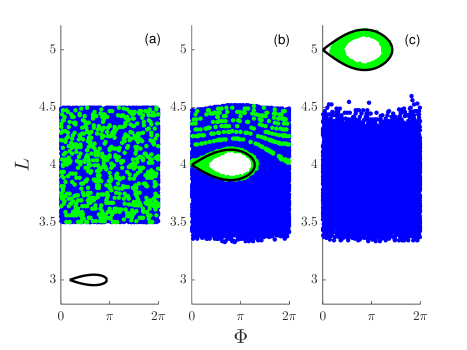
Figure 4: (Color online) Numerical simulations (single resonance approximation) for $10^{4}$ molecules distributed uniformly between $L=3.5$ and $4.5$ initially with $C=4$. The panels show the distribution of the ensemble at three consecutive times (in terms of the normalized driving frequency): $\omega_{d}=3$ (a),$4$ (b) and $5$ (c). Green and blue circles show resonantly trapped and untrapped molecules, respectively, and the black lines are the associated separatrixes. The parameters are $P_{1}=0.63$ and $P_{2}=10$. $\Phi$ is shifted so that $\Phi=0$ is at the saddle point of panel (c). A video of the simulation is provided in the online supplementary material movie .

The resonant phase space dynamics shown in Fig. 4 can be explained on the bases of (a) the adibaticity in the problem landau and (b) the incompressibility of the phase space Goldstein-inco . The adiabaticity guarantees the conservation of the area of the empty hole inside the growing separatrix, while the incompressibility of the phase space ensures that the distribution of the newly trapped molecules inside the separatrix would be the same uniform (original) distribution as long as $L_{r}$ is well within the range $L_{1},L_{2}$. Therefore, as time progresses and the resonant separatrix passes an infinitesimal distance $\delta L_{r}$ inside the distribution, the density $\delta N$ of newly trapped molecules is

$$\delta N=P\delta S=P\frac{\partial S}{\partial L_{r}}\delta L_{r},$$ (19)

where $P$ is the initial (uniform) density of the molecules in phase space and $\delta S$ is the change of the area of separatrix during the corresponding infinitesimal time interval. Thus, the number of the newly trapped molecules after passage through the whole distribution is $\Delta N=P\Delta S$, $\Delta S$ being the full added area of the separatrix after the passage. These simple arguments also allow us to calculate the probability of capture into resonance for a general initial distribution of $L$ and $C$, (i.e. $L_{z}$), which will be discussed next.

III.3 Capture Probability

The generalization to the case of an arbitrary initial phase space density distribution $P(L,C)$ independent of $\Phi$ can proceed by viewing this distribution as a collection of uniform infinitesimally thin layers, each having some value of $C$. As the most prevailing case, we focus on initially thermal distribution of molecules, where the distribution of $L$ is

$$P_{th}\left(L\right)=L\exp{\left(-\frac{L^{2}}{2}\right)},$$ (20)

and, therefore,

$$P(L,C)=\left\{\begin{array}[]{ccc}0&,&L<C/2\\ \frac{NP_{th}\left(L\right)}{4\pi L}&,&L>C/2\end{array}\right.,$$ (21)

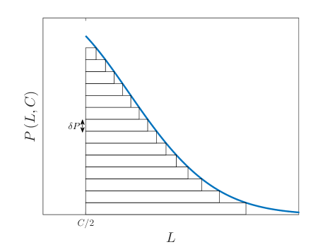
Figure 5: Phase space density distribution $P(L,C)$ viewed as a collection of uniform layers of height $\delta P$ each.

where $N$ is the density of the molecules. For a given $C$, we view this distribution as a collection of uniform layers of thickness $\delta P$ as illustrated in Fig. 5. The resonant drive passes all these layers, so at any given time, we have a collection of identical separatrices around the resonant $L_{r}$. Since the layers have a uniform density, and $\Delta L\ll 1$, the passage of the separatrix through the layers can be treated as discussed above. As the separatrix advances an infinitesimal distance $\delta L_{r}$, the total density (after summation over all the layers and integration over $\Phi$) of newly trapped molecules for given $C$ will be [see Eq. (19)]

$$\delta N\left(L_{r},C\right)=P(L_{r},C)\frac{\partial S}{\partial L_{r}}\delta L_{r}.$$ (22)

Next, we integrate (22) over $C$ and change the integration from $C$ to $R=L_{z}/L=1-C/L_{r}$, which is uniformly distributed between $-1,1$ to get

$$\delta N(L_{r})=\delta L_{r}\frac{NP_{th}\left(L\right)}{4\pi L}\int_{-1}^{1}\frac{dS}{dR}\left(1-R\right)dR.$$ (23)

Finally, we collect the newly trapped molecules as the resonant $L_{r}$ passes from some initial $L_{r0}$ to a final value $L_{rf}$ (the normalized driving frequency varies from $\omega_{0}$ to $\omega_{f}$) to get the density of all newly resonantly trapped molecules

$$\Delta N=\int_{L_{r0}}^{L_{rf}}\frac{NP_{th}\left(L\right)}{4\pi L}dL_{r}\int_{-1}^{1}\frac{dS}{dR}\left(1-R\right)dR.$$ (24)

After integrating in $R$ (by parts) and in $L_{r}$, the last expression becomes

$$\Delta N=\sqrt{\frac{\pi}{2}}\frac{NQ}{4\pi}\left[erf\left(\chi_{f}\right)-erf\left(\chi_{0}\right)\right],$$ (25)

where $\chi=L_{r}/\sqrt{2}=\omega_{d}/\left(\sqrt{2}\omega_{th}\right)$ and $Q=\int_{-1}^{1}SdR$ is the total ”volume” of the separatrix in the 3-dimensional extended phase-space which includes the $R$ dimension. To get the total density of trapped molecules, we must add the density of the initially trapped molecules, which, for $\Delta L\ll 1$ is

$$\Delta N_{0}=\frac{QN}{4\pi}P_{th}\left(\omega_{0}\right)\text{.}$$ (26)

Then the total capture probability in the problem is

$$P_{cap}=\frac{Q}{4\pi}\left\{\sqrt{\frac{\pi}{2}}\left[erf\left(\chi_{f}\right)-erf\left(\chi_{0}\right)\right]+P_{th}\left(\omega_{0}\right)\right\}.$$ (27)

Finally, $Q$ in the last equation can be found numerically via

$$Q=\frac{\sqrt{2}}{P_{2}}\int_{-1}^{1}dR\int_{\Delta\Phi}\sqrt{D\left(1-\cos{\Phi}\right)+\sin{\Phi}-\Phi}d\Phi,$$ (28)

where $D=\sqrt{[4P_{1}P_{2}V\left(R\right)]^{2}-1}$, $\Delta\Phi$ is the width of the separatrix in $\Phi$, and we shifted $\Phi$ in (28) so that $\Phi=0$ is at the saddle point. Note that $Q$ depends on $P_{2}$ and the product $P_{1}P_{2}$ and, therefore, for a given $\omega_{0},\omega_{f}$, the capture probability scales with temperature as $T^{-1/2}$ via $P_{2}$. Furthermore, asymptotically for large $P_{1}P_{2}$, $Q$ $\sim\sqrt{P_{1}/P_{2}}$, which is independent of the chirp rate $\beta$.

IV Results and Discussion

We illustrate our theory in Fig. 6, where the prediction of Eq. (27) is compared with numerical simulations (single resonance approximation). We applied the OC drive to a thermal ensemble for parameters $P_{1}=1.58$, $P_{2}=10$. The final normalized driving frequency in  this example was $8$, while the initial normalized driving frequency was varied. One observes an excellent agreement of the theory (black line) with simulations. Note that counter-intuitively, when $\omega_{0}$ decreases and $P_{th}\left(\omega_{0}\right)$ becomes small, the capture probability increases and reaches a maximum. In these cases, the vast majority of captured molecules cross the separatrix during the evolution, and don’t start in resonance initially.

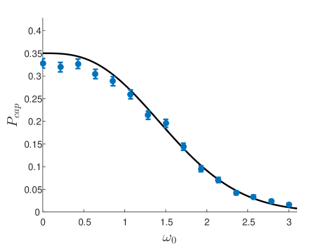
Figure 6: Monte Carlo simulations (single resonance approximation) of the resonant capture probability of initially thermal ensemble (2000 molecules), versus the initial normalized driving frequency $\omega_{0}$. The solid line is the analytic result [see Eq. (27)]. The parameters are $P_{1}=1.58$, $P_{2}=10$ and $\omega_{f}=8$.

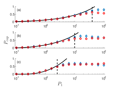
Figure 7: (Color online) The resonant capture probability for three equal $P_{2}$ lines in $P_{1,2}$ parameter space in Fig. 8. The red circles show full simulation in original spherical coordinates, blue diamonds are single resonance simulations, and analytic result is shown by the solid line. The parameters are $P_{2}=39.8$ (a), $10$ (b) and $2.51$ (c), $\omega_{0}=1$ and $\omega_{f}=5$. Dashed lines show the location of the weak drive limit. The number of molecules in simulations ranges from 500 to 5000, but the numerical uncertainty in all cases is smaller than the marker size.

Additional results are presented in Fig. 7, testing a broader range of parameters. In each panel in the figure, the OC drive with normalized frequency varying from $\omega_{0}=1$ to $\omega_{f}=5$ is applied to a thermal ensemble and $P_{2}$ is kept constant at $39.8$ (a), $10$ (b) and $2.51$ (c), while $P_{1}$ is varied. The numerical results include the simulations in spherical coordinates (blue diamonds), the single resonance simulations (red circles), and both are compared with the analytical result (solid line). One can see that the analytic prediction correctly describes the simulations only in a certain range of parameters. This is not surprising, as several approximations were made in the theory, and need to be discussed next. One such approximation is the relative smallness $\Delta L\ll 1$ of the width of the separatrix in $L$. In terms of parameters $P_{1,2},$ this condition yields inequality

$$\sqrt{P_{1}/P_{2}}\ll 1,$$ (29)

which justifies the approximation in Eq. (13). In addition, we used the single resonance assumption, allowing to discard higher nonresonant harmonic contribution in deriving Eq. (5), which requires $P_{1}/P_{2}\ll 1$ and is guaranteed by (29). The location of $P_{1}=P_{2}$ is shown in Fig. 7 by dashed lines and one can see that both types of simulations agree until one violates condition $P_{1}/P_{2}\ll 1$, but the theoretical curves deviate earlier, because condition (29) is stricter. The ratio $P_{1}/P_{2}$ measures the relative strength of the drive, so Eq. (29) describes the weak drive limit.

Another assumption of the theory is the adiabaticity of autoresonant evolution, i.e. $\nu^{-2}d\nu/d\tau\ll 1$, where $\nu=\sqrt{4P_{1}P_{2}V}$ is the characteristic frequency of autoresonant modulations (oscillations of trajectories trapped inside the separatrix). We estimate $d\nu/d\tau\sim O(\sqrt{P_{1}P_{2}}dL_{r}/dt)\sim O(\sqrt{P_{1}/P_{2}})$ and, therefore the adiabaticity is guaranteed if

$$P_{2}P_{1}^{1/3}\gg 1.$$ (30)

Note that the resonant capture is impossible when there is no separatrix (no trapped trajectories) for all $C$ values, which leads to the condition

$$P_{1}P_{2}>1/2$$ (31)

for trapping. While this condition doesn’t affect the validity of the results, it provides a useful border in $P_{1,2}$ parameter space. We summarize this analysis in Fig 8 showing the $P_{1,2}$ parameter space with boundaries defined by the above conditions as black solid lines and the region of validity of the analytic results in color with the color map corresponding to the theoretical capture probability for $\omega_{0}=1$ and $\omega_{f}=5$. The black diamond in the figure shows the conditions of experiments milner1 ; milner2 ; milner5 ($E_{0}\approx 4.3\cdot 10^{9}\,\text{volt/m}$, $\beta\approx 1.7\times 10^{24}\,sec^{-2}$ for $O_{2}$ molecules at room temperature), which are in the region of validity of the theory. The red dashed lines mark the parameter range in simulations in Fig. 7, while the blue triangles show the conditions of simulations in Fig. 1 with panel (c) in this figure way outside the weak drive limit.

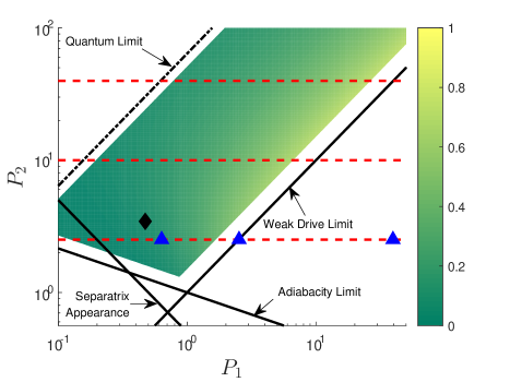
Figure 8: (Color online) Validity conditions in $P_{1,2}$ parameter space. The color coding represents the capture probability for a drive with $\omega_{0}=1$, $\omega_{f}=5$. The black lines are the weak drive limit (Eq. 29), location of formation of separatrix (Eq. 31), and the adiabacity condition (Eq. 30). The dashed-dot black line is an example of the quantum limit for $O_{2}$ at room temperature. The horizontal red dashed lines represent the values of $P_{1,2}$ simulated in Fig 7. The blue triangles are the parameters used in Fig. 1, while the red diamond shows parameters used in experiments milner1 ; milner2 ; milner5 .

At this stage, we discuss the assumed classicality of our system. The classical thermal distribution (20) is valid only when the most probable $j$, the quantum number associated with the total angular momentum, in the thermal equilibrium is large , say $j_{th}>5$. In addition, the dynamics of trapped molecules must be classical. For this to be true, the characteristic area $S$ (dimensional) of the separatrix in phase space must exceed the Planck’s constant $h$, so mixing of a few angular momentum states would be possible. Then, the inequality $\sqrt{P_{2}/P_{1}}<j_{th}$ can serve as a condition for classicality of trapped trajectories. An example of this condition is presented in Fig. 8 by the dot-dashed line for $O_{2}$ at room temperature. Unlike the rest of the above conditions, this line is not fixed in the $P_{1,2}$ space, and is both temperature and molecule dependent via $j_{th}$ ($j_{th}=8$ in the figure). Note that the classical results presented in this work are in the range of typical OC experiments. Note also that the conservation law $L-L_{z}=const$ in our theory is the classical counterpart of the OC quantum selection rule $\left|j,m\right\rangle\rightarrow\left|j+2,m+2\right\rangle$, where $m$ is the magnetic quantum number girard .

Finally, in developing the theory, we have assumed that the characteristic parameters $P_{1,2}$ are constant. In typical experiments these parameters may vary in time. For example, the laser pulse amplitude may have slow temporal dependence, the chirp rate $\beta$ may vary in time, and the trapped molecules may experience slow centrifugal expansion at high rotation speeds. Because of the adiabaticity, these effects can be taken into account within our theory by using instantaneous values of $P_{1,2}$. For example, the adiabaticity guarantees continued trapping in the system as long as $P_{1}P_{2}V$ (see Eq. 16) is an increasing function of time.  If  this function starts to decrease because of the aforementioned variation of parameters, some molecules can escape the trapping. This effect of ”leaked molecules” was recently observed experimentally milner1 ; milner2 . Note that this leakage can be stopped by slowly increasing the driving amplitude, i.e. $P_{1}$ in time.

V SUMMARY

In conclusion, we have studied the process of capture of an ensemble of molecules into resonance in the optical centrifuge and calculated the associated capture probability. Based on three characteristic time scales in the problem, we have introduced two dimensionless parameters $P_{1,2}$ (see Eqs. (1) and (2)), transformed the problem to action-angle representation, and applied the single resonance approximation in our analysis, allowing a significant acceleration of numerical simulations. We have then studied the continuous phase space dynamics of the reduced one degree of freedom system and found the probability of filling of separatrix by newly trapped molecules. This calculation was based on the adiabaticity in the problem and the incompressibility of the phase-space, avoiding the complex issue of deciding the fate of individual trajectories. For a thermal ensemble, we have compared the analytic results with numerical simulations, showing excellent agreement, provided one satisfies the weak drive limit, the adiabaticity and the classicality conditions, which were mapped in $P_{1,2}$ parameter space. It is shown that these conditions hold in current experimental setups. The results of this work can be used in analysing existing and planning future experiments. It also seems important to generalize the theory into the quantum regime and study the transition from the quantum ladder climbing to the classical autoresonance AR6a ; AR9 in the problem of molecular rotations. Finally, a similar phase space analysis can be applied in studying the problem of capture into autoresonance in other dynamical systems.

Appendix A

The transformation to action-angle variables discussed in Sec. (II) is carried out similarly to Goldstein-trans ; rydberg-atom . We proceed by solving the Hamilton-Jacobi equation in the problem, to obtain the generating function Goldstein-trans

$$W(L,L_{z},\varphi,\theta)=\pm\int\sqrt{L^{2}-\frac{L_{z}^{2}}{\sin^{2}\theta}}d\theta+\varphi L_{z},$$ (32)

where the actions are the angular momentum $L$ and its projection $L_{z}$ on the $Z$-axix, the integration is along the trajectory, and the choice of the sign accounts for the difference between the ascending and descending nodes. The canonical transformation equations in this case are:

$$p_{\varphi} =\frac{\partial W}{\partial\varphi} = L_{z},$$ (33)

$$p_{\theta} =\frac{\partial W}{\partial\theta} = \pm\sqrt{L^{2}-\frac{L_{z}^{2}}{\sin^{2}\theta}},$$ (34)

$$\Theta_{L} =\frac{\partial W}{\partial L} = \pm\int\frac{L\sin\theta}{\sqrt{L^{2}\sin^{2}\theta-L_{z}^{2}}}d\theta,$$ (35)

$$\Theta_{L_{z}} =\frac{\partial W}{\partial L_{z}} = \mp\int\frac{L_{z}}{\sin^{2}\theta}\frac{1}{\sqrt{L^{2}-\frac{L_{z}^{2}}{\sin^{2}\theta}}}d\theta+\varphi.$$ (36)

It has been shown in Goldstein-trans that the angles $\Theta_{L},\Theta_{L_{z}}$ are two of the Euler angles, $\Theta_{L}$ measures the rotation of the molecule in its plane of rotation, while $\Theta_{L_{z}}$ measures the precession of the rotation plane itself. Substitution of the first two transformation equations into the unperturbed Hamiltonian yields

$$H_{0}=P_{2}L^{2}/2.$$ (37)

For calculating the perturbed part of the Hamiltonian we set $\Theta_{L}=0$ when $\theta$ is at its minimal value, and $\Theta_{L_{z}}=0$ when the line of nodes is along the $X$ axis, and solve the integrals in Eq. (35), (36) to find:

$$\cos{\theta} =\sqrt{1-L_{z}^{2}/L^{2}}\cos{\Theta_{L}},$$ (38)

$$\varphi =\Theta_{L_{z}}+\arctan[{(L/L_{z})\tan{\Theta_{L}]}}+\frac{\pi}{2}.$$ (39)

Next, we define $s=signL_{z}$ and notice that $\arctan{\left(L/L_{z}\tan{\Theta_{L}}\right)}$ can be written as the sum $s\Theta_{L}+sf\left(\left|L/L_{z}\right|,\Theta_{L}\right)$, where $f$ is a periodic function of $\Theta_{L}$ of period $\pi$. We expand this function in Fourier series to get

$$f\left(\left|L/L_{z}\right|,\Theta_{L}\right)=\sum_{n=1}^{\infty}\frac{\left(\left|L/L_{z}\right|-1\right)^{n}}{n\left(\left|L/L_{z}\right|+1\right)^{n}}\sin{\left(2n\Theta_{L}\right)},$$ (40)

which, in terms of $A=\left(\left|L/L_{z}\right|-1\right)/\left(\left|L/L_{z}\right|+1\right),$ becomes:

$$f\left(\left|L/L_{z}\right|,\Theta_{L}\right)=-\frac{i}{2}\log\left(\frac{1-Ae^{-2i\Theta_{L}}}{1-Ae^{2i\Theta_{L}}}\right).$$ (41)

At this point, we write the action-angle representation of the perturbed part of the Hamiltonian using Eqs. (38), (39):

$$U=\left[\left(1-L_{z}^{2}/L^{2}\right)\cos^{2}\Theta_{L}-1\right]\sin^{2}\Psi,$$ (42)

where $\Psi=\Theta_{L_{z}}+s\Theta_{L}+sf-\phi_{d}$ and then use Eq. (41) to find the closed form expressions for $\cos\left(2f\right),\sin\left(2f\right)$. We define the phase mismatch $\Phi=2(\Theta_{L}+\Theta_{L_{z}}-\phi_{d})$ in the problem, use this definition to replace $2(\Theta_{L_{z}}-\phi_{d})$ in (42) and average the resulting $U(L_{z}/L,\Theta_{L},\Phi)$ with respect to the fast phase $\Theta_{L}$. This yields the full Hamiltonian in the single resonance approximation:

$$H\left(\Theta_{L},\Theta_{L_{z}},L,L_{z}\right)\approx P_{2}\frac{L^{2}}{2}+P_{1}V\cos{\Phi}+P_{1}F,$$ (43)

where

$$V = \frac{1}{8}\left(1+\frac{L_{z}}{L}\right)^{2},$$ (44)

$$F = \frac{1}{4}\left(1-\frac{{L_{z}}^{2}}{L^{2}}\right).$$ (45)

Note that this result is independent of $s$ and that angle $\Theta_{L}$ exhibits non-trivial behavior, as it always increases, regardless the direction of rotation (given by $s$).

References

- (1) I. S. Averbukh and R. Arvieu, Phys. Rev. Lett. 87, 163601 (2001).
- (2) F. Rosca-Pruna and M. J. J. Vrakking, Phys. Rev. Lett. 87, 153902 (2001).
- (3) J. M. Rost, J. C. Griffin, B. Friedrich, and D. R. Herschbach, Phys. Rev. Lett. 68, 1299 (1992).
- (4) M. J. J. Vrakking and S. Stolte, Chem. Phys. Lett. 271, 209 (1997).
- (5) K. Kitano, H. Hasegawa, and Y. Ohshima, Phys. Rev. Lett. 103, 223002 (2009).
- (6) S. Fleischer, Y. Khodorkovsky, Y. Prior and I. S Averbukh, New J. Phys. 11, 105039 (2009).
- (7) S. Zhdanovich, A. A. Milner, C. Bloomquist, J. Floss, I. Sh. Averbukh, J.W. Hepburn, and V. Milner, Phys. Rev. Lett. 107, 243004 (2011).
- (8) J. Karczmarek, J. Wright, P. Corkum, and M. Ivanov, Phys. Rev. Lett. 82, 3420 (1999).
- (9) D. M. Villeneuve, S. A. Aseyev, P. Dietrich, M. Spanner, M.Yu. Ivanov, and P. B. Corkum, Phys. Rev. Lett. 85, 542 (2000).
- (10) R. Hasbani, B. Ostojic, P.R. Bunker, and M.Y. Ivanov, J. Chem. Phys. 116, 10636 (2002).
- (11) K. Tilford, M. Hoster, P.M. Florian, and R. C. Forrey, Phys. Rev. A 69, 052705 (2004).
- (12) Y. Khodorkovsky, J. R. Manson, and I. Sh. Averbukh, Phys. Rev. A 84, 053420 (2011).
- (13) U. Steinitz, Y. Prior and I.S Averbukh, Phys. Rev. Lett. 112, 013004 (2014).
- (14) U. Steinitz, Y. Prior and I.S Averbukh, Phys. Rev. Lett. 109, 033001 (2012).
- (15) L. Yuan, S.W. Teitelbaum, A. Robinson and A.S. Mullin, Proc. Natl. Acad. Sci. U.S.A. 108, 17 (2011).
- (16) A. Korobenko, A.A. Milner and V. Milner, Phys. Rev. Lett. 112, 113004 (2014).
- (17) A.A. Milner, A. Korobenko, J.W. Hepburn and V. Milner, Phys. Rev. Lett. 113, 043005 (2014).
- (18) A.A. Milner, A. Korobenko, K. Rezaiezadeh and V. Milner, Phys. Rev. X 5, 031041 (2015).
- (19) A.A. Milner, A. Korobenko and V. Milner, Optics Express 23, 7 (2015).
- (20) M. Spanner and M.Y. Ivanov, J. Chem. Phys. 114, 3456 (2001).
- (21) M. Spanner, K.M. Davitt, and M.Y. Ivanov, J. Chem. Phys. 115, 8403 (2001).
- (22) N.V. Vitanov and B. Girard, Phys. Rev. A 69, 033409 (2004).
- (23) B. Meerson and L. Friedland, Phys. Rev. A 41, 5233 (1990).
- (24) W. K. Liu, B. Wu, and J. M. Yuan, Phys. Rev. Lett. 75, 1292 (1995).
- (25) J. Fajans, E. Gilson, and L. Friedland, Phys. Rev. Lett. 82, 4444 (1999).
- (26) J. Fajans, E. Gilson, and L. Friedland, Phys. Plasmas 6, 4497 (1999).
- (27) L. Friedland, Phys. Rev. E 59, 4106 (1999).
- (28) G. Manfredi and P.A. Hervieux, Appl. Phys. Lett. 91, 061108 (2007).
- (29) G. Marcus, L. Friedland, and A. Zigler, Phys. Rev. A 69, 013407 (2004).
- (30) Y. Shalibo, Y. Rofe, I. Barth, L. Friedland, R. Bialczack, J.M. Martinis, and N. Katz, Phys. Rev. Lett. 108, 037701 (2012).
- (31) I. Barth and L. Friedland, Phys. Rev. Lett. 113, 040403 (2014).
- (32) B. V. Chirikov, Phys. Reports 52, 265 (1979).
- (33) J. Fajans, E. Gilson, and L. Friedland, Phys. Rev. E 62, 4131 (2000).
- (34) A. I. Neishtadt, in Mathematics and modelling, Ed. A. Bazykin and Yu. Zarkhin (Nova Sci. Publ., Commack, NY, 1993) pp. 199-226.
- (35) See Supplemental Material at [URL comes here] for a video of the simulation in Fig. 4.
- (36) L. Friedland, P. Khain, and A. G. Shagalov, Phys. Rev. Lett. 96, 225001 (2006).
- (37) L. D. Landau and E. M. Lifshits, Mechanics (Pergamon Press, Oxford, 1976) pp. 154-157.
- (38) H. Goldstein, Classical Mechanics (Addison-Wesley, Reading, MA, 1980) pp. 426-428.
- (39) A.A. Milner, A. Korobenko and V. Milner, N. J. Phys. 16, 093038 (2014).
- (40) I. Barth and L. Friedland, Phys. Rev. A 87, 053420 (2013).
- (41) H. Goldstein, Classical Mechanics (Addison-Wesley, Reading, MA, 1980) pp. 472-483.
- (42) E. Grosfeld and L. Friedland, Phys. Rev. E 65 , 046230 (2002).