Kershaw closures for linear transport equations in slab geometry II: high-order realizability-preserving discontinuous-Galerkin schemes

Abstract

This paper provides a generalization of the realizability-preserving discontinuous-Galerkin scheme given in [3] to general full-moment models that can be closed analytically. It is applied to the class of Kershaw closures, which are able to provide a cheap closure of the moment problem. This results in an efficient algorithm for the underlying linear transport equation. The efficiency of high-order methods is demonstrated using numerical convergence tests and non-smooth benchmark problems.

1 Introduction

Moment closures are a class of spectral methods used in the context of kinetic transport equations. An infinite set of moment equations is defined by taking velocity- or phase-space averages with respect to some basis of the velocity space. A reduced description of the kinetic density is then achieved by truncating this hierarchy of equations at some finite order. The remaining equations however inevitably require information from the equations which were removed. The specification of this information, the so-called moment closure problem, distinguishes different moment methods. In the context of linear radiative transport, the standard spectral method is commonly referred to as the $\text{P}_{N}$ closure [24], where $N$ is the degree of the highest-order moments in the model. The $\text{P}_{N}$ method is powerful and simple to implement, but does not take into account the fact that the original function to be approximated, the kinetic density, must be non-negative. Thus $\text{P}_{N}$ solutions can contain negative values for the local densities of particles, rendering the solution physically meaningless.

Entropy-based moment closures, referred to as $\text{M}_{N}$ models in the context of radiative transport [25, 9], have all the properties one would desire in a moment method, namely positivity of the underlying kinetic density, hyperbolicity of the closed system of equations, and entropy dissipation [22]. Practical implementation of these models has been traditionally considered too expensive because they require the numerical solution of an optimization problem at every point on the space-time grid, but recently there has been renewed interest in the models due to their inherent parallelizability [15]. However, while their parallelizability goes a long way in making $\text{M}_{N}$ models computationally competitive, in order to make these methods truly competitive with more basic discretizations, the gains in efficiency that come from higher-order methods (in space and time) will likely be necessary. Here the issue of realizability becomes a stumbling block.

The property of positivity implies that the system of moment equations only evolves on the set of so-called realizable moments. Realizable moments are simply those moments associated with positive densities, and the set of these moments forms a convex cone which is a strict subset of all moment vectors. This property, while indeed desirable since it is consistent with the original kinetic density, can cause problems for numerical methods. Standard high-order numerical solutions (in space and time) to the Euler equations, which indeed are an entropy-based moment closure, have been observed to have negative local densities and pressures [44]. Similar effects have been reported in the context of elastic flow [30]. This is exactly loss of realizability.

A recently popular high-order method for hyperbolic systems is the Runge-Kutta discontinuous Galerkin (RKDG) method [5, 6, 7]. An RKDG method for moment closures can handle the loss of realizability through the use of a realizability (or “positivity-preserving”) limiter [44], but so far these have been implemented for low-order moment systems (that is $N=1$ or $2$) [26] because here one can rely on the simplicity of the structure of the realizable set for low-order moments. For moments of large order $N$, the realizable set has complex nonlinear boundaries: when the velocity domain is one-dimensional, the realizable set is characterized by the positive-definiteness of Hankel matrices [37, 8]; in higher dimensions, the realizable set is not well understood. In [3], using that a quadrature-based approximation of the realizable set is a convex polytope [1], the realizability limiters of [44, 26] has been generalized for moment systems of (in principle) arbitrary order.

To avoid the expensive minimum-entropy ansatz a new hierarchy of full-moment models has been derived in [31], the class of Kershaw closures, based on the findings in [17]. It provides a reasonably simple closure relation, closely related to minimum-entropy models while being cheap to evaluate. This paper aims at generalizing the scheme given in [3] to this class of models for (in principle) arbitrary moment order $N$.

This paper is organized as follows. First, the transport equation and its moment approximations are given. Then, the available realizability theory is shortly reviewed, followed by a brief summary of the class of Kershaw closures. The discontinuous-Galerkin scheme is given with the necessary extensions to obtain a realizability-preserving scheme. Numerical convergence of this scheme up to seventh order against an analytical solution is shown and the Kershaw closures are submitted to a set of benchmark tests investigating the effect of high-order space-time approximations. Finally, conclusions and an outlook on future work is given.

2 Modelling

In slab geometry, the transport equation under consideration has the form

$$\partial_{t}\psi+\mu\partial_{z}\psi+\sigma_{a}\psi=\sigma_{s}\mathcal{C}\left(\psi\right)+Q,\qquad t\in T,z\in X,\mu\in[-1,1].$$ (2.1)

The physical parameters are the absorption and scattering coefficient $\sigma_{a},\sigma_{s}:T\times X\to\mathbb{R}_{\geq 0}$, respectively, and the emitting source $Q:T\times X\times[-1,1]\to\mathbb{R}_{\geq 0}$. Furthermore, $\mu\in[-1,1]$, and $\psi=\psi(t,z,\mu)$.

The shorthand notation $\left<\cdot\right>=\int\limits_{-1}^{1}\cdot~{}d\mu$ denotes integration over $[-1,1]$.

Assumption 2.1.

Following [21], the collision operator $\mathcal{C}$ is assumed to have the following properties.

2. Mass conservation

   $$\left<\mathcal{C}\left(\psi\right)\right>=0.$$ (2.2a)

3. Local entropy dissipation

   $$\left<\eta^{\prime}(\psi)\mathcal{C}\left(\psi\right)\right>\leq 0,$$ (2.2b)

   where $\eta$ denotes a strictly convex, twice differentiable entropy.

4. Constants in the kernel:

   $$\mathcal{C}\left(c\right)=0\qquad\text{for every }c\in\mathbb{R}.$$ (2.2c)

A typical example for $\mathcal{C}$ is the linear integral operator

$$\mathcal{I}\left(\psi\right)=\int\limits_{-1}^{1}K(\mu,\mu^{\prime})\psi(t,z,\mu^{\prime})~{}d\mu^{\prime}-\psi(t,z,\mu),$$ (2.3)

where $K$ is non-negative, symmetric in both arguments and normalized to $\int\limits_{-1}^{1}K(\mu,\mu^{\prime})~{}d\mu^{\prime}=1$. In this paper the special case of the BGK-type isotropic-scattering operator with $K\equiv\frac{1}{2}$ is used for the simulations.

(2.1) is supplemented by initial and boundary conditions:

$$\psi(0,z,\mu) =\psi_{t=0}(z,\mu) \text{for }z\in X=(z_{L},z_{R}),\mu\in[-1,1],$$ (2.4a)

$$\psi(t,z_{L},\mu) =\psi_{b}(t,z_{L},\mu) \text{for }t\in T,\mu>0,$$ (2.4b)

$$\psi(t,z_{R},\mu) =\psi_{b}(t,z_{R},\mu) \text{for }t\in T,\mu<0.$$ (2.4c)

3 Moment models and realizability

In general, solving equation (2.1) is very expensive in two and three dimensions due to the high dimensionality of the state space.

For this reason it is convenient to use some type of spectral or Galerkin method to transform the high-dimensional equation into a system of lower-dimensional equations. Typically, one chooses to reduce the dimensionality by representing the angular dependence of $\psi$ in terms of some basis ${\mathbf{b}}$.

Definition 3.1.

The vector of functions ${\mathbf{b}}:[-1,1]\to\mathbb{R}^{N+1}$ consisting of $N+1$ basis functions $b_{i}$, $i=0,\ldots N$ of maximal order $N$ is called an angular basis.

The so-called moments of a given distribution function $\psi$ with respect to ${\mathbf{b}}$ are then defined by

$$\mathbf{u}=\left<{{\mathbf{b}}}\psi\right>=\left(u_{0},\ldots,u_{N}\right)^{T},$$ (3.1)

where the integration is performed componentwise.

Assuming for simplicity $b_{0}\equiv 1$, the quantity $u_{0}=\left<b_{0}\psi\right>=\left<\psi\right>$ is called local particle density. Furthermore, normalized moments $\boldsymbol{\phi}=\left(\phi_{1},\ldots,\phi_{N}\right)\in\mathbb{R}^{N}$ are defined as

$$\boldsymbol{\phi}=\cfrac{\left<{\widehat{\mathbf{b}}}\psi\right>}{\left<\psi\right>}~{},$$ (3.2)

where ${\widehat{\mathbf{b}}}=\left(b_{1},\ldots,b_{N}\right)^{T}$ is the remainder of the basis ${\mathbf{b}}$.

To obtain a set of equations for $\mathbf{u}$, (2.1) has to be multiplied through by ${\mathbf{b}}$ and integrated over $[-1,1]$, giving

$$\left<{\mathbf{b}}\partial_{t}\psi\right>+\left<{\mathbf{b}}\partial_{z}\mu\psi\right>+\left<{\mathbf{b}}\sigma_{a}\psi\right>=\sigma_{s}\left<{\mathbf{b}}\mathcal{C}\left(\psi\right)\right>+\left<{\mathbf{b}}Q\right>.$$

Collecting known terms, and interchanging integrals and differentiation where possible, the moment system has the form

$$\partial_{t}\mathbf{u}+\partial_{z}\left<\mu{\mathbf{b}}\hat{\psi}_{\mathbf{u}}\right>+\sigma_{a}\mathbf{u}=\sigma_{s}\left<{\mathbf{b}}\mathcal{C}\left(\hat{\psi}_{\mathbf{u}}\right)\right>+\left<{\mathbf{b}}Q\right>.$$ (3.3)

The solution of (3.3) is equivalent to the one of (2.1) if ${\mathbf{b}}$ is a basis of $L_{2}(\mathcal{S}^{2},\mathbb{R})$.

Since it is impractical to work with an infinite-dimensional system, only a finite number of $N+1<\infty$ basis functions ${\mathbf{b}}$ of order $N$ can be considered. Unfortunately, there always exists an index $i\in\{0,\dots,N\}$ such that the components of $b_{i}\cdot\mu$ are not in the linear span of ${\mathbf{b}_{N}}$. Therefore, the flux term cannot be expressed in terms of $\mathbf{u}_{N}$ without additional information. Furthermore, the same might be true for the projection of the scattering operator onto the moment-space given by $\left<{\mathbf{b}}\mathcal{C}\left(\psi\right)\right>$. This is the so-called closure problem. One usually prescribes some ansatz distribution $\hat{\psi}_{\mathbf{u}}(t,\mathbf{x},\Omega):=\hat{\psi}(\mathbf{u}(t,\mathbf{x}),{\mathbf{b}}(\Omega))$ to calculate the unknown quantities in (3.3). Note that the dependence on the angular basis in the short-hand notation $\hat{\psi}_{\mathbf{u}}$ is neglected for notational simplicity.

In this paper, the full-moment monomial basis $b_{i}=\mu^{i}$ is considered. However, it is in principle possible to extend the derived concepts to other bases like half [11, 10] or mixed moments [12, 33].

The rest of this section is a brief summary of the corresponding parts in [31]. All details and further discussions can be found therein.

3.1 Realizability

Since the underlying kinetic density to be approximated is non-negative, a moment vector only makes sense physically if it can be associated with a non-negative distribution function. In this case the moment vector is called realizable.

Definition 3.2.

The realizable set $\mathcal{R}_{{\mathbf{b}}}$ is

$$\mathcal{R}_{{\mathbf{b}}}=\left\{\mathbf{u}~{}:~{}\exists\psi(\mu)\geq 0,\,\left<\psi\right>>0,\text{ such that }\mathbf{u}=\left<{\mathbf{b}}\psi\right>\right\}.$$

If $\mathbf{u}\in\mathcal{R}_{{\mathbf{b}}}$, then $\mathbf{u}$ is called realizable. Any $\psi$ such that $\mathbf{u}=\left<{\mathbf{b}}\psi\right>$ is called a representing density. If $\psi$ is additionally a linear combination of Dirac deltas [14, 41, 19], it is called atomic [8].

Definition 3.3.

Let $A,B\in\mathbb{R}^{n\times n}$ be Hermitian matrices. The partial ordering $"\geq"$ on such matrices is defined by $A\geq B$ if and only if $A-B$ is positive semi-definite. In particular $A\geq 0$ denotes that $A$ is positive semi-definite.

For the full-moment basis the question of finding practical characterizations of the realizable set $\mathcal{R}_{{\mathbf{b}}}$ has been completely solved in [8]. See [31] for more details. The following characterizations of the above realizable set holds.

Lemma 3.4.

Define the Hankel matrices

$$A(k):=\left(u_{i+j}\right)_{i,j=0}^{k},\quad B(k):=\left(u_{i+j+1}\right)_{i,j=0}^{k},\quad C(k):=\left(u_{i+j}\right)_{i,j=1}^{k}.$$

Then the realizable set satisfies

$$\mathcal{R}_{{\mathbf{b}}}=\begin{cases}\left\{\mathbf{u}\in\mathbb{R}^{N+1}~{}|~{}A(k)\geq B(k),~{}A(k)\geq-B(k)\right\}&\text{ if }$$N$=2k+1$,\\ \left\{\mathbf{u}\in\mathbb{R}^{N+1}~{}|~{}A(k)\geq 0,A(k-1)\geq C(k)\right\}&\text{ if }$$N$=2k$.\\ \end{cases}$$

Due to the structure of the used Hankel matrices (the highest moment $u_{N}$ always appears exactly once in the entries of the matrices) it is always possible to rearrange the conditions involving this highest moment in Theorem 3.4 in such a way that

$$f_{\text{up}}(u_{0},\ldots,u_{N-1})\geq u_{N}\geq f_{\text{low}}(u_{0},\ldots,u_{N-1})$$

for functions $f_{\text{up}}$ and $f_{\text{low}}$. Whenever $\mathbf{u}$ is realizable and $u_{N}=f_{\text{low}}(u_{0},\ldots,u_{N-1})$, $\mathbf{u}$ is said to be on the lower $N^{\text{th}}$-order realizability boundary. Similarly, if $u_{N}=f_{\text{up}}(u_{0},\ldots,u_{N-1})$, $\mathbf{u}$ is said to be on the upper $N^{\text{th}}$-order realizability boundary.

The functions $f_{\text{up}}$ and $f_{\text{low}}$ can be specified using the pseudoinverses of combinations of Hankel matrices. To simplify notation later, the following corollary is written in terms of $u_{N+1}$ instead of $u_{N}$.

Corollary 3.5.

The functions $f_{\text{up}}$ and $f_{\text{low}}$ satisfying

$$f_{\text{up}}(u_{0},\ldots,u_{N})\geq u_{N+1}\geq f_{\text{low}}(u_{0},\ldots,u_{N})$$ (3.4)

are given by

$$f_{\text{up}}(u_{0},\ldots,u_{N}) =\begin{cases}u_{N-1}-\boldsymbol{\beta}_{-}^{T}\left(A(k-1)-C(k-1)\right)^{\dagger}\boldsymbol{\beta}_{-}&\text{ if }N=2k+1\\ u_{N}-\boldsymbol{\beta}_{-}^{T}\left(A(k-1)-B(k-1)\right)^{\dagger}\boldsymbol{\beta}_{-}&\text{ if }N=2k\end{cases}$$

$$f_{\text{low}}(u_{0},\ldots,u_{N}) =\begin{cases}\boldsymbol{\beta}_{+}^{T}A^{\dagger}(k)\boldsymbol{\beta}_{+}&\text{ if }N=2k+1\\ -u_{N}+\boldsymbol{\beta}_{+}^{T}\left(A(k-1)+B(k-1)\right)^{\dagger}\boldsymbol{\beta}_{+}~{}&\text{ if }N=2k\end{cases}$$

where in the odd case

$$\boldsymbol{\beta}_{-}=\left(u_{k}-u_{k+2},\ldots,u_{N-2}-u_{N}\right)^{T},\qquad\boldsymbol{\beta}_{+}=\left(u_{k+1},\ldots,u_{N}\right)^{T}$$

and in the even case

$$\boldsymbol{\beta}_{\mp}=\left(u_{k}\mp u_{k+1},\ldots,u_{N-1}\mp u_{N}\right)^{T}.$$

Remark 3.6.

By convention, $\boldsymbol{\beta}_{-}^{T}\left(A(k-1)-C(k-1)\right)^{\dagger}\boldsymbol{\beta}_{-}=0$ if $N=1$.

3.2 Kershaw closures

With the previous realizability theory it is now possible to develop the closure strategy which is called Kershaw closure. This class of moment models is defined by convexly combining upper and lower moments of order $N+1$ in such a way that the isotropic point is correctly reproduced.

Corollary 3.7.

The Kershaw closure $\text{K}_{N}$ of order $N$ is given by

$$\phi_{N+1}(\boldsymbol{\phi})=\zeta f_{\text{low}}(\boldsymbol{\phi})+(1-\zeta)f_{\text{up}}(\boldsymbol{\phi}),$$ (3.5)

where the interpolation constant

$$\zeta=\cfrac{\frac{1}{2}\left<\mu^{N+1}\right>-f_{\text{up}}(\boldsymbol{\phi}_{\text{iso}})}{f_{\text{low}}(\boldsymbol{\phi}_{\text{iso}})-f_{\text{up}}(\boldsymbol{\phi}_{\text{iso}})}=\begin{cases}\frac{k+2}{2k+3}&\text{ if }N=2k+1\\ \frac{1}{2}&\text{ if }N=2k\end{cases}$$ (3.6)

is defined via the functions $f_{\text{up}}$ and $f_{\text{low}}$ as given in Corollary 3.5 and $\boldsymbol{\phi}_{\text{iso}}=\frac{\left<{\mathbf{b}}\right>}{2}$.

For convenience, (3.3) using the Kershaw closure can be written in the form of a usual first-order system of balance laws

$$\partial_{t}\mathbf{u}+\partial_{z}\mathbf{F}_{3}\left(\mathbf{u}\right)=\mathbf{s}\left(\mathbf{u}\right),$$ (3.7)

where

$$\mathbf{F}\left(\mathbf{u}\right) =\left(u_{1},\ldots,u_{N+1}\right)\in\mathbb{R}^{N+1},$$ (3.8a)

$$\mathbf{s}\left(\mathbf{u}\right) =\sigma_{s}\left(\frac{1}{2}\boldsymbol{\phi}_{\text{iso}}u_{0}-\mathbf{u}\right)+\left<{\mathbf{b}}Q\right>-\sigma_{a}\mathbf{u}.$$ (3.8b)

4 Realizability-preserving discontinuous-Galerkin scheme

Recent numerical experiments have shown that high-order schemes (in space and time) outperform highly-resolved first-order methods, comparing degrees of freedom and running time versus approximation quality. This has been investigated in the case of minimum-entropy moment models in [3, 34] for two different types of schemes. The most challenging part is to preserve realizability during the simulation since otherwise the closure cannot be evaluated. Unfortunately, higher-order schemes typically cannot guarantee this property on their own, as has been observed in the context of the compressible Euler equations (which are indeed in the hierarchy of minimum-entropy models) in [44] and for the $\text{M}_{1}$ model in [26].

Due to the lack of smoothness in the underlying distribution of the Kershaw models (since it is atomic) the application of the high-order kinetic scheme presented in [34] is not obvious. This has been observed before in [40] for quadrature-based moment methods. Therefore this paper focuses on the discontinuous-Galerkin scheme presented in [3]. While there only quadrature-based minimum-entropy models have been investigated, the following sections will show how to generalize the scheme and its realizability limiter to the general case of full-moment models.

In the following, the spatial domain $X=(z_{L},z_{R})$ is divided into (for notational simplicity) $n_{z}$ (equidistant) cells $I_{j}=(z_{j-\frac{1}{2}},z_{j+\frac{1}{2}})$, where the cell interfaces are given by $z_{j\pm\frac{1}{2}}=z_{j}\pm\frac{\Delta z}{2}$ for cell centres $z_{j}=z_{L}+(j-\frac{1}{2})\Delta z$, and $\Delta z=\frac{z_{R}-z_{L}}{n_{z}}$.

Furthermore, $P^{k}(I_{j})$ is the set of polynomials of degree at most $k$ on the interval $I_{j}$, and

$$V_{h}^{k}=\{v\in L_{1}(X):v|_{I_{j}}\in P^{k-1}(I_{j})\text{ for }j\in\{1,\ldots,n_{z}\}\}$$ (4.1)

is the finite-element space of piecewise polynomials of degree $k-1$.

The discontinuous-Galerkin method for the general hyperbolic system (3.7), as outlined in [5, 6, 7], can be briefly described as follows.

For each $t\in T$, seek an approximate solution $\mathbf{u}_{h}(t,z)$ whose components live in the finite-element space $V_{h}^{k}$ as defined in (4.1).

Then follow the Galerkin approach: replace $\mathbf{u}$ in (3.7) by a solution of the form $\mathbf{u}_{h}\in V_{h}^{k}$, multiply the resulting equation by basis functions $v_{h}$ of $V_{h}^{k}$ and integrate over cell $I_{j}$ to obtain

$$\partial_{t}\int_{I_{j}}\mathbf{u}_{h}(t,z)v_{h}(z)~{}dz +\mathbf{F}_{3}(\mathbf{u}_{h}(t,z_{j+\frac{1}{2}}^{-}))v_{h}(z_{j+\frac{1}{2}}^{-})-\mathbf{F}_{3}(\mathbf{u}_{h}(t,z_{j-\frac{1}{2}}^{+}))v_{h}(z_{j-\frac{1}{2}}^{+})$$

$$-\int_{I_{j}}\mathbf{F}_{3}(\mathbf{u}_{h}(t,z))\partial_{z}v_{h}(z)~{}dz=\int_{I_{j}}\mathbf{s}(\mathbf{u}_{h}(t,z))v_{h}(z)~{}dz,$$ (4.2a)

$$\int_{I_{j}}\mathbf{u}_{h}(0,z)v_{h}(z)~{}dz =\int_{I_{j}}\mathbf{u}_{t=0}(z)v_{h}(z)~{}dz,$$ (4.2b)

where $z_{j\pm\frac{1}{2}}^{-}$ and $z_{j\pm\frac{1}{2}}^{+}$ again denote the limits from left and right, respectively, and $\mathbf{u}_{t=0}=\left<{\mathbf{b}}\psi_{t=0}\right>$ is the projection of the initial distribution to the moment space. In order to approximately solve the Riemann problem at the cell-interfaces, the fluxes $\mathbf{F}_{3}(\mathbf{u}_{h}(t,z_{j+\frac{1}{2}}^{\pm}))$ at the points of discontinuity are both replaced by a numerical flux $\widehat{\mathbf{F}}(\mathbf{u}_{h}(t,z_{j+\frac{1}{2}}^{-}),\mathbf{u}_{h}(t,z_{j+\frac{1}{2}}^{+}))$, thus coupling the elements with their neighbours [39]. Several well-known examples for such a numerical flux $\widehat{\mathbf{F}}$ exist in literature. The simplest example is the global Lax-Friedrichs flux

$$\widehat{\mathbf{F}}(\mathbf{u}_{1},\mathbf{u}_{2})=\dfrac{1}{2}\left(\mathbf{F}_{3}(\mathbf{u}_{1})+\mathbf{F}_{3}(\mathbf{u}_{2})-C(\mathbf{u}_{2}-\mathbf{u}_{1})\right).$$ (4.3)

The numerical viscosity constant $C$ is taken as the global estimate of the absolute value of the largest eigenvalue of the Jacobian $\mathbf{F}_{3}^{\prime}$. Following [31], the viscosity constant can be set to $C=1$, because for the moment systems used here it can be shown that the largest eigenvalue is bounded in absolute value by one.

The local Lax-Friedrichs flux could be used instead. This requires computing the eigenvalues of the Jacobian in every space-time cell to adjust the value of the numerical viscosity constant $C$ but possibly decreases the overall diffusivity of the scheme. However, since high-order space-time approximations are considered, the decrease in diffusivity achieved by switching to the local Lax-Friedrichs flux should be negligible.

The usual approach is to expand the approximate solution $\mathbf{u}_{h}$ on each interval as

$$\left.\mathbf{u}_{h}\right|_{I_{j}}(t,z):=\mathbf{u}_{j}(t,z):=\sum_{i=0}^{k-1}\widehat{\mathbf{u}}_{j}^{i}(t)v_{i}\left(\frac{z-z_{j}}{\Delta z}\right),$$ (4.4)

where $v_{0},v_{1},\ldots,v_{k-1}$ denote a basis for $P^{k}(\hat{I})$ with respect to the standard $L_{2}$-scalar product on the reference cell $\hat{I}=\left(-\frac{1}{2},\frac{1}{2}\right)$. It is convenient to choose an orthogonal basis like the Legendre polynomials scaled to the interval $\hat{I}$, denoted by

$$v_{0}(\hat{z})=1,\quad v_{1}(\hat{z})=2\hat{z},\quad v_{2}(\hat{z})=\frac{1}{2}(12\hat{z}^{2}-1),\>\ldots$$ (4.5)

With an orthogonal basis the cell means $\overline{\mathbf{u}}_{j}$ are easily available from the expansion coefficients $\widehat{\mathbf{u}}_{j}^{i}$, since

$$\overline{\mathbf{u}}_{j}(t):=\frac{1}{\Delta z}\int_{I_{j}}\mathbf{u}_{j}(t,z)~{}dz=\frac{1}{\Delta z}\sum_{i=0}^{k-1}\widehat{\mathbf{u}}_{j}^{i}(t)\int_{I_{j}}v_{i}\left(\frac{z-z_{j}}{\Delta z}\right)~{}dz=\widehat{\mathbf{u}}_{j}^{0}(t).$$ (4.6)

Collecting the coefficients $\widehat{\mathbf{u}}_{j}^{i}(t)$ into the $k\times(N+1)$ matrix

$$\widehat{\mathbf{u}}_{j}(t)=\left(\widehat{\mathbf{u}}_{j}^{0}(t),\ldots,\widehat{\mathbf{u}}_{j}^{k-1}(t)\right)^{T},$$ (4.7)

equation (4.2) can be written in compact form as the coupled system of ordinary differential equations

$$\partial_{t}\widehat{\mathbf{u}}_{j} =\tilde{L}_{h}(\widehat{\mathbf{u}}_{j-1},\widehat{\mathbf{u}}_{j},\widehat{\mathbf{u}}_{j+1}),\quad\text{for }j\in\{1,\ldots,n_{z}\}\text{ and }t\in T,$$ (4.8)

with initial condition (4.2b) and an appropriate choice of the local differential operator $\tilde{L}_{h}$ [3].

The incorporation of boundary conditions for moment systems is non-trivial. Here, an often-used approach is taken that incorporates boundary conditions via ‘ghost cells’. First assume that it is possible to smoothly extend $\psi_{b}(t,z,\mu)$ in $\mu$ to $[-1,1]$ for $z\in\{z_{L},z_{R}\}$ (note that while moments are defined using integrals over all $\mu$, the boundary conditions in (2.4b)–(2.4c) are only defined for $\mu$ corresponding to incoming data).

Then the moment approximations in the ghost cells at $z_{0}$ and $z_{n_{z}+1}$ simply take the form

$$\mathbf{u}_{0}(t,z_{\frac{1}{2}}) :=\left<{\mathbf{b}}\psi_{b}(t,z_{L},\mu)\right>,$$ (4.9a)

$$\mathbf{u}_{n_{z}+1}(t,z_{n_{z}+\frac{1}{2}}) :=\left<{\mathbf{b}}\psi_{b}(t,z_{R},\mu)\right>.$$ (4.9b)

Note, however, that the validity of this approach, due to its inconsistency with the original boundary conditions (2.4b)–(2.4c), is not entirely non-controversial, but the question of appropriate boundary conditions for moment models is an open problem [27, 20, 28, 38, 23] which is not explored here.

For Dirichlet-boundary conditions, the simplest approach is taken. The ghost-cell moments are chosen to be the constant functions

$$\mathbf{u}_{0}(t,z) \equiv\mathbf{u}_{0}(t,z_{\frac{1}{2}}),$$

$$\mathbf{u}_{n_{z}+1}(t,z) \equiv\mathbf{u}_{n_{z}+1}(t,z_{n_{z}+\frac{1}{2}}),$$

with $\mathbf{u}_{0}(t,z_{\frac{1}{2}})$ and $\mathbf{u}_{n_{z}+1}(t,z_{n_{z}+\frac{1}{2}})$ defined as in (4.9).

For periodic boundary conditions, the obvious choice is

$$\mathbf{u}_{0}(t,z) =\mathbf{u}_{n_{z}}(t,z+z_{R}-z_{L}),\quad z\in I_{0},$$

$$\mathbf{u}_{n_{z}+1}(t,z) =\mathbf{u}_{1}(t,z-z_{R}+z_{L}),\quad z\in I_{n_{z}+1}.$$

All that remains to obtain a high-order scheme in space and time is a suitable time integrator for (4.8). Such a class of integrators is given by the strong-stability-preserving (SSP) methods, as used for example in [44, 2]. The stages and steps of these type of methods are convex combinations of forward-Euler steps. Since the realizable set is convex, the analysis of a forward-Euler step then suffices to prove realizability preservation of the full method.

When possible, SSP-Runge-Kutta (SSP-RK) methods are used, but unfortunately they only exist up to order four [29, 13]. For orders $k\geq 5$ the so-called two-step Runge-Kutta (TSRK) SSP methods [18] as well as their generalizations, the multi-step Runge-Kutta (MSRK) SSP methods [4] can be applied. They combine Runge-Kutta schemes with positive weights and high-order multistep methods to achieve a total order higher than four while maintaining the important SSP property.

See [34] for more information about the SSP-schemes used in the actual implementation. Note that they differ from those used in [3] where only discretizations up to third order were used, in contrast to the methods of order one to seven given in [34].

The rest of the methodology follows closely [3]. Here, the standard TVBM corrected minmod limiter proposed in [6] is used.

Assuming that the major part of the spurious oscillations is generated in the linear part of the underlying polynomial, whose slope in the reference cell is simply $\widehat{\mathbf{u}}_{j}^{1}$, a limiter can be defined as

$$\Lambda^{\text{scalar}}(\widehat{\mathbf{u}}_{j-1},\widehat{\mathbf{u}}_{j},\widehat{\mathbf{u}}_{j+1})=\left\{\begin{array}[]{cc}\left(\begin{array}[]{c}\left(\widehat{\mathbf{u}}_{j}^{0}\right)^{T}\\ m\left(\widehat{\mathbf{u}}_{j}^{1},\widehat{\mathbf{u}}_{j+1}^{0}-\widehat{\mathbf{u}}_{j}^{0},\widehat{\mathbf{u}}_{j}^{0}-\widehat{\mathbf{u}}_{j-1}^{0}\right)^{T}\\ (0,0,\ldots,0)\\ \vdots\\ (0,0,\ldots,0)\end{array}\right)&\text{ if }\left|\widehat{\mathbf{u}}_{j}^{1}\right|\geq M(\Delta z)^{2},\\ \widehat{\mathbf{u}}_{j}&\text{otherwise},\end{array}\right.$$ (4.17)

for the $j^{\text{th}}$ cell and the case $k\geq 3$, that is piece-wise quadratic or higher-degree polynomials, so that the final rows of zeros in the first case indicates that the coefficients for the higher-order spatial basis functions $v_{1},\ldots,v_{k-1}$ are set to zero for each moment component. The absolute value and the inequality are applied componentwise. The label “scalar” is used because the limiter is directly applied to each scalar component of $\widehat{\mathbf{u}}_{h}{}$. The function $m\left(\cdot\right)$ is the standard minmod function applied componentwise, defined by

$$m\left(a_{1},a_{2},a_{3}\right) =\begin{cases}\operatorname{sign}(a_{1})\min\{|a_{1}|,|a_{2}|,|a_{3}|\}&\text{if }\operatorname{sign}(a_{1})=\operatorname{sign}(a_{2})=\operatorname{sign}(a_{3}),\\ 0&\text{else}.\end{cases}$$

The constant $M$ is a problem-dependent estimate of the second derivative, though it has to be noted that in [6] the authors did not find the solutions very sensitive to the value chosen for this parameter.

However, it has been found that applying the limiter to the components themselves may introduce non-physical oscillations around an otherwise monotonic solution [5]. Instead, the limiter is applied to the local characteristic fields of the solution. The flux Jacobian is obtained numerically using finite differences. This can be achieved cheaply since only the last equation of the flux has to be considered, all other components are trivial.

4.1 Realizability preservation

In order to evaluate the flux-term $\mathbf{F}_{3}(\mathbf{u}_{h}(t,z))$ at the spatial quadrature nodes $z_{j,\upsilon}$ in the $j^{\text{th}}$ cell, at least $\mathbf{u}_{j}(z_{j,\upsilon})=:\mathbf{u}_{j,\upsilon}\in\mathcal{R}_{{\mathbf{b}}}$ for each node is necessary.

To prove Theorem 4.2 the following rather strong assumption has to be made.

Assumption 4.1.

For every $\psi$ satisfying $\mathbf{u}=\left<{\mathbf{b}}\psi\right>$ there exists a $\widetilde{\mathbf{u}}\in\mathcal{R}_{{\mathbf{b}}}$ such that the moments of the collision operator $\mathcal{C}$ with respect to the same angular basis ${\mathbf{b}}$ can be written as

$$\left<{\mathbf{b}}\mathcal{C}\left(\psi\right)\right>=\widetilde{\mathbf{u}}-\mathbf{u}.$$ (4.18)

This assumption is fulfilled by the integral collision operator (2.3).

While first-order schemes (like the Lax-Friedrichs method) automatically preserve realizability of the cell means [3], higher-order schemes ($k\geq 2$) typically cannot guarantee this property on their own, as has been observed in the context of the compressible Euler equations (which are indeed in the hierarchy of minimum-entropy models) in [44] and for the $\text{M}_{1}$ model in [26].

It is, however, possible to show that, when the moments at the quadrature nodes are realizable, the presented schemes preserve realizability of the cell means $\overline{\mathbf{u}}_{j}(t)$ under a CFL-type condition. With realizable cell means available, a point-wise-realizable polynomial representation can be obtained by applying a linear scaling limiter which pushes $\mathbf{u}_{j,\upsilon}$ towards the cell mean and thus into the realizable set for each quadrature node $z_{j,\upsilon}$.

Following the arguments in [43, 42], this limiter does not destroy the accuracy of the scheme in case of smooth solutions if $\overline{\mathbf{u}}_{j}$ is not on the boundary of the realizable set. This is verified numerically in Section 5.1. For convenience, the main result of [3, 34] is summarized in the following theorem. Note that, since SSP time integrators are used, it suffices to investigate forward Euler steps in time, which are then convexly combined to obtain the designed order of time integration in the SSP scheme.

Theorem 4.2 ([3, 34]).

Assume that

1. for all cells $j\in\{1,2,\ldots,n_{z}\}$ it holds that $0\leq Q(t_{\kappa},z),\sigma_{a}(t_{\kappa},z),\sigma_{s}(t_{\kappa},z)\in V_{h}^{k_{s}}$, $k_{s}\in\mathbb{N}$;

2. the cell means $\overline{\mathbf{u}}_{j}^{\left(\kappa\right)}$ at time step $t_{\kappa}$ are realizable;

3. at the quadrature nodes of the ${n_{\Upsilon}}$-point Gauss-Lobatto rule on each cell $I_{j}$, ${n_{\Upsilon}}=\left\lceil\frac{k+k_{s}+1}{2}\right\rceil$, the point-wise values of the moment approximation $\mathbf{u}_{h}$ (componentwise in $V_{h}^{k}$) are realizable.

Then under the CFL condition

$$\Delta t<\min\left(\cfrac{1}{\sigma_{t}^{\max}},\cfrac{\Delta z\hat{w}_{1}}{1+\Delta z\hat{w}_{1}\sigma_{t}^{\max}}\right),$$ (4.19)

the cell means $\overline{\mathbf{u}}_{j}^{\left(\kappa+1\right)}$ after one forward-Euler step are realizable, where

$$\sigma_{t}^{\max}:=\max\limits_{\begin{subarray}{c}j\in\{1,\ldots,n_{z}\}\\ \upsilon\in\{1,\ldots,{n_{\Upsilon}}\}\end{subarray}}\sigma_{t}\left(t_{\kappa},z_{j,\upsilon}\right).$$ (4.20)

All that remains is to ensure that assumption (iii) in Theorem 4.2 is always fulfilled. Due to assumption (ii) and the convexity of the realizable set, this can be achieved using a linear-scaling limiter, pushing the polynomial representation towards the (realizable) cell mean. This approach has been outlined in [44, 43, 45] for the Euler equations and in [3] for two classes of minimum-entropy models.

For ease of notation, time indices are dropped.

Recall the definition (4.4) of $\mathbf{u}_{j}$, given by

$$\mathbf{u}_{j}(z)=\overline{\mathbf{u}}_{j}+\sum_{i=1}^{k-1}\widehat{\mathbf{u}}_{j}^{i}v_{i}\left(\frac{z-z_{j}}{\Delta z}\right).$$

Due to the convexity of the realizable set, if $\overline{\mathbf{u}}_{j}$ is realizable, then for each quadrature point there exists a $\theta\in[0,1]$ such that

$$\mathbf{u}_{j}^{\theta}(z_{j,\upsilon}):=\mathbf{u}_{j,\upsilon}^{\theta}:=\theta\overline{\mathbf{u}}_{j}+(1-\theta)\mathbf{u}_{j,\upsilon}$$ (4.21)

is realizable. Indeed, by inserting the definition of $\mathbf{u}_{j}(z_{j,\upsilon})$ from above, the limited moment vector can be written as

$$\mathbf{u}_{j,\upsilon}^{\theta}=\overline{\mathbf{u}}_{j}+\left(1-\theta\right)\sum_{i=1}^{k-1}\widehat{\mathbf{u}}_{j}^{i}v_{i}\left(\frac{z_{j,\upsilon}-z_{j}}{\Delta z}\right),$$

thus when limiting is necessary, the higher-order coefficients $\widehat{\mathbf{u}}_{j}^{i}$, $i=1,\ldots,k-1$, are damped while the cell mean remains unchanged.

The task of the limiter is now to choose for each $\mathbf{u}_{j}$ the minimal value of $\theta_{j}\in[0,1]$ such that $\mathbf{u}_{j}^{\theta_{j}}$ is realizable at all quadrature nodes $z_{j,\upsilon}$. This choice is optimal in the sense that the least information of the original polynomial is lost ($\theta=0$ corresponds to no limiting while $\theta=1$ resembles limiting to first order).

Remark 4.3.

For readability reasons, the dependence on the cell index $j$ is dropped sometimes throughout the following examples.

Having the non-linear structure of the full realizable set $\mathcal{R}_{{\mathbf{b}}}$ in mind, computing the smallest $\theta$ such that $\mathbf{u}_{j,\upsilon}^{\theta}\in\mathcal{R}_{{\mathbf{b}}}$ requires some effort.

Theorem 4.4.

The solution to the limiter problem

$$\min~{} \theta$$

s.t. $$\mathbf{u}_{j,\upsilon}^{\theta}\in\mathcal{R}_{{\mathbf{b}}}$$

$$\theta\in[0,1]$$

requires to calculate the roots of two polynomials of degree at most $N$.

Proof.

Assume that $N=2k+1$. Define $\overline{A}$, $A$, $\overline{B}$ and $B$ to be the Hankel matrices associated with $\overline{\mathbf{u}}_{j}$ and $\mathbf{u}_{j}(z_{j,\upsilon})$, respectively. Then the Hankel matrices associated with $\mathbf{u}_{j,\upsilon}^{\theta}$ are

$$A^{\theta}:=\theta\overline{A}+(1-\theta)A,$$

$$B^{\theta}:=\theta\overline{B}+(1-\theta)B.$$

By assumption (compare Lemma 3.4), $\overline{A}\geq\pm\overline{B}$. This implies that all eigenvalues of $\overline{A}\mp\overline{B}$ are non-negative, and therefore $\det\left(\overline{A}\mp\overline{B}\right)\geq 0$. Being on the realizability boundary corresponds to having at least one zero eigenvalue, which is equivalent to a vanishing determinant of either $A^{\theta}-B^{\theta}$ or $A^{\theta}+B^{\theta}$. Note that $\det\left(A^{\theta}\pm B^{\theta}\right)$ is a polynomial of degree $N$ in $\theta$. Since the realizable set is convex, the maximal $\theta$ in $[0,1]$ that is a root of one of the two polynomials is the optimal limiter value.

The case $N=2k$ works analogously. ∎

Example 4.5.

Realizability conditions for $N=1$ are very simple: $u_{0}\geq\pm u_{1}$. Plugging in $\mathbf{u}^{\theta}$ from (4.21) gives

$$\theta\overline{u}_{0}+\left(1-\theta\right)u_{0}\geq\pm\theta\overline{u}_{1}\pm\left(1-\theta\right)u_{1}.$$

Solving these equations for equality (which is equivalent to finding roots of a polynomial of degree $N=1$) results in

$$\theta_{\pm}=\frac{u_{0}\mp u_{1}}{u_{0}\mp u_{1}-\overline{u}_{0}\pm\overline{u}_{1}}.$$

Example 4.6.

For $N=2$ the realizability conditions are given through the Hankel matrices

$$A(0)=u_{0},~{}C(1)=u_{2},~{}A(1)=\begin{pmatrix}u_{0}&u_{1}\\ u_{1}&u_{2}\end{pmatrix}$$

and the conditions $A(1)\geq 0$ and $A(0)\geq C(1)$. The matrices defining the limiter value $\theta$ are given by

$$D_{1}(\theta) =A^{\theta}(0)-C^{\theta}(1)=\theta(\overline{u}_{0}-\overline{u}_{2})+(1-\theta)(u_{0}-u_{2}),$$

$$D_{2}(\theta) =A^{\theta}(1)=\theta\begin{pmatrix}\overline{u}_{0}&\overline{u}_{1}\\ \overline{u}_{1}&\overline{u}_{2}\end{pmatrix}+(1-\theta)\begin{pmatrix}u_{0}&u_{1}\\ u_{1}&u_{2}\end{pmatrix}.$$

The required polynomials are given by $p_{1,2}(\theta)=\det\left(D_{1,2}(\theta)\right)$, i.e.

$$p_{1}(\theta) =\theta(\overline{u}_{0}-\overline{u}_{2})+(1-\theta)(u_{0}-u_{2})$$

$$p_{2}(\theta) =\left(-{u_{1}}^{2}+2\,u_{1}\,\overline{u}_{1}-{\overline{u}_{1}}^{2}-u_{2}\,\overline{u}_{0}+\overline{u}_{0}\,\overline{u}_{2}+u_{0}\,\left(u_{2}-\overline{u}_{2}\right)\right)\,\theta^{2},$$

$$\quad+\left(2\,{u_{1}}^{2}-2\,\overline{u}_{1}\,u_{1}+u_{2}\,\overline{u}_{0}-u_{0}\,\left(2\,u_{2}-\overline{u}_{2}\right)\right)\,\theta+\left(u_{0}\,u_{2}-{u_{1}}^{2}\right).$$

Let e.g. $\overline{\mathbf{u}}=\left(1,0,\frac{1}{3}\right)^{T}$ and $\mathbf{u}=\left(1,\frac{4}{5},\frac{1}{5}\right)^{T}$. Then it follows that

$$p_{1}(\theta) =\frac{4}{5}-\frac{2}{15}\theta,$$

$$p_{2}(\theta) =-\frac{11}{25}+\frac{106}{75}\theta-\frac{16}{25}\theta^{2},$$

which have roots $\theta_{1}=6$, $\theta_{2+}=\frac{11}{6}$ and $\theta_{2-}=\frac{3}{8}$. Since $\theta_{1},\theta_{2+}\notin[0,1]$ it follows that $\theta=\theta_{2-}$ and $\mathbf{u}^{\theta}=\left(1,\frac{1}{2},\frac{1}{4}\right)^{T}$, which indeed satisfies the second-order realizability condition $u_{2}^{\theta}u_{0}^{\theta}\geq u_{1}^{\theta}u_{1}^{\theta}$ with equality. This example is visualized in Figure 1.

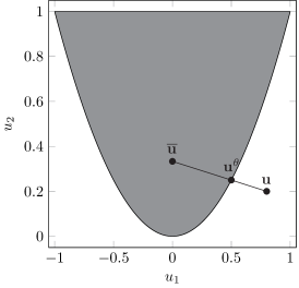
Figure 1: Limiter example for the second-order basis with $u_{0}=1$. The realizable set is plotted in grey.

Remark 4.7.

To analytically obtain the coefficients for the resulting polynomials in $\theta$ is in general hard. However, this can be avoided using a simple trick. In the odd case evaluate the determinants of $A^{\theta}\pm B^{\theta}$ at $N+1$ distinct values of $\theta$, e.g. at the $N+1$ linearly-spaced values in $[0,1]$. These points uniquely define the desired polynomial. A similar approach can be done in the even case.

Remark 4.8.

It has been shown in [32] that the slope limiter (4.17) (either evaluated in primitive or conserved variables) always has to be applied before the realizability limiter since the application of the slope limiter may destroy point-wise realizability (and thus Theorem 4.2 cannot be applied).
Both limiters have to be applied at every stage and step of the SSP time integrators.

5 Numerical experiments

This section contains numerical convergence results and some often-used benchmark problems for moment models. They serve as a reference for the efficiency of Kershaw closures with a high number of moments combined with high-order space-time discretizations.

The approximations of highest order in space and time are discretized with $k=7$ on a grid with $50$ cells, the medium order is represented by a $k=4$ solution on a grid with $100$ cells and the first-order variant is calculated on a grid with $500$ cells. If not stated otherwise the TVB constant in the modified minmod limiter is set to $M=5$ for $k=7$ and $M=20$ for $k=4$ (compare [6, 3]).

5.1 Convergence results

5.1.1 Manufactured solution

In general, obtaining analytical solutions for moment models is a hard task. In the case of Kershaw closures it is possible to provide a solution in some special cases. Consider the initial distribution

$$\psi_{t=0}(z,\mu)=f(z)\delta\left(\mu-1\right)$$

with some positive $f(z)>0$. Setting $\sigma_{a}=\sigma_{s}=0$, the analytical solution of the transport equation (2.1) is given by

$$\psi_{a}(t,z,\mu)=f(z-t)\delta\left(\mu-1\right).$$

On the moment level this corresponds to a linear advection with transport speed $1$ since

$$u_{a,i}(t,z)=\left<\mu^{i}\psi_{a}(t,z,\mu)\right>=f(z-t)\qquad\text{ for all }i\in\{0,\ldots,N\}.$$

Since $\delta\left(\mu-1\right)$ can be reproduced exactly by the Kershaw closures [31] the moments of the transport solution are also the moments of the Kershaw closure if $N\geq 1$. For this example the local mass is defined as $f(z)=\sin(z)$ on $X=[-\pi,\pi]$. The final time is set to $t_{f}=0.2\pi$ and periodic boundary conditions are applied.

Errors are computed in the zeroth moment of the solution $u_{a,0}(t,z):=\left<\psi_{a}(t,z,\cdot)\right>$. Then $L_{1}$- and $L_{\infty}$-errors for the zeroth moment $u_{h,0}(t,z)$ (that is, the zeroth component of a numerical solution $\mathbf{u}_{h}$) are defined as

$$E_{h}^{1}=\int_{X}\left|u_{a,0}(t_{f},z)-u_{h,0}(t_{f},z)\right|~{}dz\quad\mbox{and}\quad E_{h}^{\infty}=\max_{z\in X}\left|u_{a,0}(t_{f},z)-u_{h,0}(t_{f},z)\right|,$$ (5.1)

respectively. The integral in $E_{h}^{1}$ is approximated using a 100-point Gauss-Lobatto quadrature rule over each spatial cell $I_{j}$, and $E_{h}^{\infty}$ is approximated by taking the maximum over these quadrature nodes. The observed convergence order $\nu$ is defined by

$$\frac{E_{h_{1}}^{p}}{E_{h_{2}}^{p}}=\left(\frac{\Delta z_{1}}{\Delta z_{2}}\right)^{\nu},$$ (5.2)

where $E_{h_{i}}^{p}$, $i\in\{1,2\}$, $p\in\{1,\infty\}$, is the $L_{p}$-error $E_{h}^{p}$ for the numerical solution using cell size $\Delta z_{i}$.

A convergence table for orders $k\in\{2,4,5,6,7\}$ is presented in Table 1.

	$k=2$			$k=4$			$k=5$			$k=6$			$k=7$
$n_{z}$	$E_{h}^{1}$		$\nu$	$E_{h}^{1}$		$\nu$	$E_{h}^{1}$		$\nu$	$E_{h}^{1}$		$\nu$	$E_{h}^{1}$		$\nu$
10	7.	721e-02	—	1.	418e-04	—	4.	449e-06	—	1.	235e-07	—	2.	595e-09	—
20	2.	168e-02	1.8	9.	004e-06	4.0	1.	430e-07	5.0	1.	898e-09	6.0	2.	107e-11	6.9
40	1.	017e-02	1.1	5.	788e-07	4.0	4.	465e-09	5.0	2.	951e-11	6.0	1.	715e-13	6.9
80	2.	580e-03	2.0	3.	667e-08	4.0	1.	401e-10	5.0	4.	629e-13	6.0	5.	961e-14	1.5
160	6.	467e-04	2.0	2.	296e-09	4.0	4.	408e-12	5.0	3.	028e-14	3.9	1.	159e-13	-1.0
$n_{z}$	$E_{h}^{\infty}$		$\nu$	$E_{h}^{\infty}$		$\nu$	$E_{h}^{\infty}$		$\nu$	$E_{h}^{\infty}$		$\nu$	$E_{h}^{\infty}$		$\nu$
10	5.	978e-02	—	1.	864e-04	—	6.	520e-06	—	1.	750e-07	—	4.	422e-09	—
20	1.	592e-02	1.9	1.	155e-05	4.0	2.	106e-07	5.0	2.	836e-09	5.9	3.	451e-11	7.0
40	4.	737e-03	1.7	7.	225e-07	4.0	6.	603e-09	5.0	4.	470e-11	6.0	3.	051e-13	6.8
80	1.	180e-03	2.0	4.	517e-08	4.0	2.	046e-10	5.0	7.	745e-13	5.9	5.	906e-14	2.4
160	2.	930e-04	2.0	2.	841e-09	4.0	6.	321e-12	5.0	9.	459e-14	3.0	5.	729e-14	0.0

Table 1: $L_{1}$- and $L_{\infty}$-errors and observed convergence order $\nu$ for the $\text{K}_{1}$ analytical solution.

It can be observed that the expected convergence rates are achieved both in $L_{1}$- and $L_{\infty}$-errors. Note that the high-order methods ($k\geq 5$) stop converging at an $L_{\infty}$-error of magnitude $10^{-14}$. This is also visible in Figure 2, where orders up to $k=7$ are plotted together with their corresponding optimal convergence rates (black dashed line).

In Figure 2 the $L_{\infty}$-error versus the computation time (computed on a Intel Core i$7$ CPU with $2.8$ GHz on a single thread) is shown. Here it is clearly visible that efficiency rises with increasing order $k$.

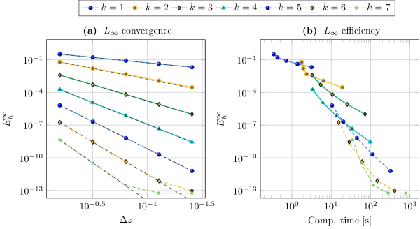
Figure 2: Convergence results in $L_{\infty}$-norm for different spatial orders and $N=1$. Black dashed lines represent the expected convergence.

Similar results can be observed using $N>1$ (tested for $N\in\{2,3\}$) but in this extreme case (the moments are always on the first-order realizability boundary) the closure procedure is more prone to numerical errors reducing the overall accuracy.

5.1.2 Investigation of the realizability limiter

Despite choosing a manufactured solution close to the boundary of realizability, the realizability limiter was not consistently active in the previous simulations. Therefore in this section an artificially-defined curve of moment vectors in space is given, and reconstructed in the finite-element space $V_{h}^{2}$ of discontinuous quadratic polynomials. Finally, the realizability limiter is used to move the reconstruction back into the set of numerically-realizable moments $\mathcal{R}_{{\mathbf{b}}}$. The convergence of this limited reconstruction is measured as before. This test case has been used before in [3] for quadrature-based minimum-entropy models. Using the Dirac-delta distribution $\delta=\delta(\mu)$, two moment vectors

$$\mathbf{u}_{0} :=(1-\gamma)\left<{\mathbf{b}}\delta(\mu-1)\right>+\gamma\mathbf{u}_{\text{iso}}=(1-\gamma){\mathbf{b}}(1)+\gamma\mathbf{u}_{\text{iso}},$$

$$\mathbf{u}_{1} :=10^{-8}\left((1-\gamma)\left<{\mathbf{b}}\delta(\mu+1)\right>+\gamma\mathbf{u}_{\text{iso}}\right)=10^{-8}\left((1-\gamma){\mathbf{b}}(-1)+\gamma\mathbf{u}_{\text{iso}}\right)$$

are chosen, which can lie arbitrarily close to the boundary of the numerically-realizable set. The parameter $\gamma\in[0,1]$ controls the distance to the boundary. For $N>1$, both $\mathbf{u}_{0}$ and $\mathbf{u}_{1}$ lie on the boundary of the realizable set when $\gamma=0$. By definition, $\mathbf{u}_{0}$ and $\mathbf{u}_{1}$ (and any convex combination thereof) are in $\mathcal{R}_{{\mathbf{b}}}$ for $\gamma\in[0,1]$, and so a realizable curve of moments in space is defined by taking convex combinations of $\mathbf{u}_{0}$ and $\mathbf{u}_{1}$, i.e.

$$\mathbf{u}(z):=(1-\zeta(z))\mathbf{u}_{0}+\zeta(z)\mathbf{u}_{1},\quad z\in[-1,1],$$ (5.3)

where $\zeta(z)\in[0,1]$ is chosen to be

$$\zeta(z):=\frac{\cos(\pi z)+1}{2},\quad z\in[-1,1].$$

To perform the convergence test, $\mathbf{u}(z)$ is projected onto $V_{h}^{2}$ and $V_{h}^{3}$ for increasing numbers of cells $n_{z}$. Then the realizability limiter is applied to ensure a realizable polynomial representation. Errors and observed convergence orders are computed as in (5.1) and (5.2), respectively. Numerical experiments show that taking $\gamma\in[0,10^{-2}]$ places the moment curve $\mathbf{u}(z)$ close enough to the boundary of realizability that the realizability limiter is active for every considered number of cells.

	$k=2$								$k=3$
$n_{z}$	$E_{h}^{1}$		$\nu$	$E_{h}^{\infty}$		$\nu$	$\theta_{\max}$		$E_{h}^{1}$		$\nu$	$E_{h}^{\infty}$		$\nu$	$\theta_{\max}$
10	9.	226e-03	—	3.	095e-02	—	3.	287e-01	4.	895e-04	—	1.	025e-03	—	8.	388e-03
20	2.	192e-03	2.1	8.	096e-03	1.9	3.	320e-01	5.	545e-05	3.1	1.	276e-04	3.0	2.	108e-03
40	5.	255e-04	2.1	2.	047e-03	2.0	3.	329e-01	6.	745e-06	3.0	1.	608e-05	3.0	5.	276e-04
80	1.	286e-04	2.0	5.	131e-04	2.0	3.	331e-01	8.	373e-07	3.0	2.	014e-06	3.0	1.	319e-04
160	3.	182e-05	2.0	1.	284e-04	2.0	3.	331e-01	1.	045e-07	3.0	2.	519e-07	3.0	3.	292e-05

Table 2: $L_{1}$- and $L_{\infty}$-errors and observed convergence order $\nu$ for the zeroth moment of the realizability-limited, piece-wise linear and quadratic reconstructions of $U(z)$ from (5.3) with $\gamma=10^{-3}$ and $N=3$.

In Table 2 convergence rates are shown for $\gamma=10^{-3}$ and the $\text{K}_{3}$ model. These results show the designed convergence order. In this table the column $\theta_{\max}$ is included, which gives the maximum value of $\theta$ from the realizability limiter over all spatial cells. The non-zero $\theta_{\max}$ in each row indicates that the realizability limiter is active for every reconstruction. Similar results can be observed for every moment component. Note that for $k\geq 4$ the realizability limiter is no longer active since the approximation quality of the reconstruction is already too good.

5.2 Plane source

In this test case an isotropic distribution with all mass concentrated in the middle of an infinite domain $z\in(-\infty,\infty)$ is defined as initial condition, i.e.

$$\psi_{t=0}(z,\mu)=\psi_{\text{vac}}+\delta(z),$$

where the small parameter $\psi_{\text{vac}}=0.5\times 10^{-8}$ is used to approximate a vacuum. In practice, a bounded domain must be used which is large enough that the boundary should have only negligible effects on the solution. For the final time $t_{f}=1$, the domain is set to $X=[-1.2,1.2]$ (recall that for all presented models the maximal speed of propagation is bounded in absolute value by one).

At the boundary the vacuum approximation

$$\psi_{b}(t,z_{L},\mu)\equiv\psi_{\text{vac}}\quad\mbox{and}\quad\psi_{b}(t,z_{R},\mu)\equiv\psi_{\text{vac}}$$

is used again. Furthermore, the physical coefficients are set to $\sigma_{s}\equiv 1$, $\sigma_{a}\equiv 0$ and $Q\equiv 0$.

In contrast to [3] a smoothed version of the Dirac is used, similar to [36], given by

$$\psi_{t=0}(z,\mu)=\psi_{\text{vac}}+\frac{1}{2\sqrt{\pi\sigma}}\exp\left(-\frac{z^{2}}{4\sigma}\right),$$

with $\sigma=3.2\cdot 10^{-4}$. To avoid a flattening of the otherwise smooth solution due to the minmod limiter the TVB constant is chosen to be $M=\infty$, completely disabling the slope limiter (but not the realizability limiter).

Some solutions at the final time are shown in Figure 3, calculated for different spatial orders and resolutions.

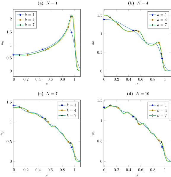
Figure 3: Local particle density $u_{0}$ in the plane-source test case for different spatial and moment orders.

It is visible that despite its much higher resolution ($500$ cells) the first-order solution is a lot more diffusive than the higher-order results ($k=4$ with $100$ and $k=7$ with $50$ cells). The medium- and high-order solution largely agree though the fourth-order one appears to be slightly more diffusive. This is the case for all presented moment orders.

The activity of the realizability limiter during the simulation is presented in Figure 4. The value of the limiter variable $\theta$ is plotted in a $z-t$ diagram showing that the limiter is most active along the shock front. This is consistent with the results in [3] where a similar test has been done for minimum-entropy models. Similarly, increasing the moment order increases the limiter activity by affecting more cells and having higher values in total.

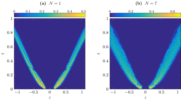
Figure 4: Realizability-limiter value $\theta$ depending on $z$ and $t$ in the plane-source test for $k=4$.

5.3 Source beam

Finally, a discontinuous version of the source-beam problem from [16] is presented. The spatial domain is $X=[0,3]$, and

$$\sigma_{a}(z)=\begin{cases}1&\text{ if }z\leq 2,\\ 0&\text{ else},\end{cases}\quad\sigma_{s}(z)=\begin{cases}0&\text{ if }z\leq 1,\\ 2&\text{ if }1<z\leq 2,\\ 10&\text{ else}\end{cases}\quad Q(z)=\begin{cases}1&\text{ if }1\leq z\leq 1.5,\\ 0&\text{ else},\end{cases}$$

with initial and boundary conditions

$$\psi_{t=0}(z,\mu)\equiv\psi_{\text{vac}},$$

$$\psi_{b}(t,z_{L},\mu)=\cfrac{e^{-10^{5}(\mu-1)^{2}}}{\left<e^{-10^{5}(\mu-1)^{2}}\right>}\quad\mbox{and}\quad\psi_{b}(t,z_{R},\mu)\equiv\psi_{\text{vac}}.$$

The final time is $t_{f}=2.5$ and the same vacuum approximation $\psi_{\text{vac}}$ as in the plane-source problem is used.

Some solutions at the final time are shown in Figure 5, calculated for different spatial orders and resolutions.

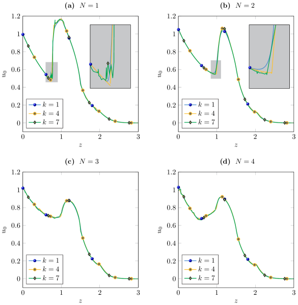
Figure 5: Local particle density $u_{0}$ in the source-beam test case for different spatial and moment orders with zoom-ins.

In this non-smooth test case the benefit of high order in space and time is slightly diminished close to discontinuities. Even more, the seventh-order solution oscillates strongly close to the shock in the $\text{K}_{1}$ solution. This is due to the modified minmod limiter, which is not capable to deal with such high-degree polynomials. Still, the fourth-order solution, calculated on a finer grid, is less diffusive than the first-order result. This is demonstrated in the close-up (grey box). The smoother the solution (which corresponds to increasing moment order $N$) the less oscillating the seventh-order solution. Furthermore, the different spatial approximations approach each other.

6 Conclusions and outlook

In this paper the necessary generalizations of the realizability-preserving discontinuous-Galerkin scheme presented in [3] for full-moment models were derived and applied to the class of Kershaw closures. These models provide a huge gain in efficiency compared to the state-of-the-art minimum-entropy models, since they can be closed (in principle) analytically using the available realizability theory. Using high-order approximations in space and time allowed to further increase this efficiency as demonstrated in a numerical convergence test and multiple benchmark problems.

Future work will have to investigate how to adapt this scheme for different scattering operators like the slightly more complicated (in terms of realizability preservation) Laplace-Beltrami operator. Furthermore, implicit-explicit schemes should be taken into account removing the drawback that the resulting CFL condition depends on the physical parameters $\sigma_{s}$ and $\sigma_{a}$. Additionally, more sophisticated slope-limiters have to be implemented to further reduce the oscillations due to the minmod limiter.

Finally, the concepts have to be lifted to higher dimensions. While fully three-dimensional first-order variants of Kershaw closures exist [17, 35], no higher-order models or a completely closed theory is available. With this, generalizing the presented scheme is in principle possible and it can be expected that similar efficiency results hold true.

Appendix A Nomenclature

Symbol	Use	First occurrence
$u_{i}$	$i$-th scalar moment	(3.1)
$\mathbf{u}$	Moment vector, either in $\mathbb{R}^{N+1}$ or the solution of (3.3)	(3.1)
$\boldsymbol{\phi}$	Normalized moment vector, in $\mathbb{R}^{N}$	(3.2)
$\mathbf{u}_{h}$	Discretized solution of (3.3), a vector of piecewise polynomials	(4.2)
$\mathbf{u}_{j}$	Restriction of $\mathbf{u}_{h}$ to the $j$-th cell, a vector of polynomials	(4.4)
$\widehat{\mathbf{u}}_{j}^{i}$	$i$-th coefficient vector (in $\mathbb{R}^{N+1}$) of the polynomial $\mathbf{u}_{j}$ wrt. the Legendre basis	(4.4)
$\overline{\mathbf{u}}_{j}$	Cell mean of the $j$-th vector of polynomials	(4.6)
$\widehat{\mathbf{u}}_{j}$	Collection of all coefficient vectors $\widehat{\mathbf{u}}_{j}^{i}$ in the $j$-th cell	(4.7)
$\mathbf{u}_{j,\upsilon}$	Evaluation of $\mathbf{u}_{j}$ at the quadrature node $z_{j,\upsilon}$	Section 4.1
$\mathbf{u}_{j}^{\theta}$	Realizability-limited version of $\mathbf{u}_{j}$	(4.21)
$\mathbf{u}_{j,\upsilon}^{\theta}$	Evaluation of $\mathbf{u}_{j}^{\theta}$ at the quadrature node $z_{j,\upsilon}$	(4.21)

References

- [1] G. W. Alldredge, C. D. Hauck, D. P. O’Leary, and A. L. Tits, Adaptive change of basis in entropy-based moment closures for linear kinetic equations, Journal of Computational Physics, 258 (2014), pp. 489–508.
- [2] G. W. Alldredge, C. D. Hauck, and A. L. Tits, High-Order Entropy-Based Closures for Linear Transport in Slab Geometry II: A Computational Study of the Optimization Problem, SIAM Journal on Scientific Computing, 34 (2012), pp. B361–B391.
- [3] G. W. Alldredge and F. Schneider, A realizability-preserving discontinuous Galerkin scheme for entropy-based moment closures for linear kinetic equations in one space dimension, Journal of Computational Physics, 295 (2015), pp. 665–684.
- [4] C. Bresten, S. Gottlieb, and Z. Grant, Strong Stability Preserving Multistep Runge-Kutta Methods, arXiv preprint, (2013).
- [5] B. Cockburn, S.-Y. Lin, and C.-W. Shu, TVB Runge-Kutta local projection discontinuous Galerkin finite element method for conservation laws III: One-dimensional systems, Journal of Computational Physics, 84 (1989), pp. 90–113.
- [6] B. Cockburn and C.-W. Shu, TVB Runge-Kutta local projection discontinuous Galerkin finite element method for conservation laws. II. General framework, Mathematics of Computation, 52 (1989), pp. 411–411.
- [7] , The Runge-Kutta Local Projection P1- Discontinuous Galerkin Method for Scalar Conservation Laws, M2AN, 25 (1991), pp. 337–361.
- [8] R. Curto and L. Fialkow, Recursiveness, positivity, and truncated moment problems, Houston J. Math, 17 (1991), pp. 603–636.
- [9] B. Dubroca and J.-L. Feugeas, Entropic Moment Closure Hierarchy for the Radiative Transfer Equation, C. R. Acad. Sci. Paris Ser. I, 329 (1999), pp. 915–920.
- [10] B. Dubroca, M. Frank, A. Klar, and G. Thömmes, Half space moment approximation to the radiative heat transfer equations, ZAMM, 83 (2003), pp. 853–858.
- [11] B. Dubroca and A. Klar, Half-moment closure for radiative transfer equations, Journal of Computational Physics, 180 (2002), pp. 584–596.
- [12] M. Frank, H. Hensel, and A. Klar, A fast and accurate moment method for the Fokker-Planck equation and applications to electron radiotherapy, SIAM Journal on Applied Mathematics, 67 (2007), pp. 582–603.
- [13] S. Gottlieb, On High Order Strong Stability Preserving Runge–Kutta and Multi Step Time Discretizations, Journal of Scientific Computing, 25 (2005), pp. 105–128.
- [14] S. Hassani, Mathematical Methods - For Students of Physics and Related Fields, Springer New York, 2nd ed., 2009.
- [15] C. D. Hauck, High-order entropy-based closures for linear transport in slab geometry, Commun. Math. Sci. v9, (2010).
- [16] C. D. Hauck, M. Frank, and E. Olbrant, Perturbed, entropy-based closure for radiative transfer, SIAM Journal on Applied Mathematics, 6 (2013).
- [17] D. S. Kershaw, Flux Limiting Nature’s Own Way: A New Method for Numerical Solution of the Transport Equation, (1976).
- [18] D. I. Ketcheson, Step sizes for strong stability preservation with downwind-biased operators, SIAM Journal on Numerical Analysis, 49 (2011), pp. 1649–1660.
- [19] H.-H. Kuo, Introduction to Stochastic Integration, Springer, 2006.
- [20] E. W. Larsen and G. C. Pomraning, The PN Theory as an Asymptotic Limit of Transport Theory in Planar Geometry —I: Analysis, Nuclear Science and Engineering, 109 (1991), pp. 49–75.
- [21] C. D. Levermore, Moment closure hierarchies for kinetic theories, Journal of Statistical Physics, 83 (1996), pp. 1021–1065.
- [22] , Moment closure hierarchies for the Boltzmann-Poisson Equation, Journal of Statistical Physics, 83 (1996), pp. 1021–1065.
- [23] , Boundary conditions for moment closures, Institute for Pure and Applied Mathematics University of California, Los Angeles, CA on May, 27 (2009).
- [24] E. E. Lewis and J. W. F. Miller, Computational Methods in Neutron Transport, John Wiley and Sons, New York, 1984.
- [25] G. N. Minerbo, Maximum entropy Eddington factors, J. Quant. Spectrosc. Radiat. Transfer, 20 (1978), pp. 541–545.
- [26] E. Olbrant, C. D. Hauck, and M. Frank, A realizability-preserving discontinuous Galerkin method for the M1 model of radiative transfer, Journal of Computational Physics, 231 (2012), pp. 5612–5639.
- [27] G. C. Pomraning, Variational boundary conditions for the spherical harmonics approximation to the neutron transport equation, Annals of Physics, 27 (1964), pp. 193–215.
- [28] R. P. Rulko, E. W. Larsen, and G. C. Pomraning, The PN Theory as an Asymptotic Limit of Transport Theory in Planar Geometry —II: Numerical Results, Nuclear Science and Engineering, 109 (1991), pp. 76–85.
- [29] S. J. Ruuth and R. J. Spiteri, High-Order Strong-Stability-Preserving Runge–Kutta Methods with Downwind-Biased Spatial Discretizations, SIAM Journal on Numerical Analysis, 42 (2004), pp. 974–996.
- [30] C. Schär and P. K. Smolarkiewicz, A Synchronous and Iterative Flux-Correction Formalism for Coupled Transport Equations, Journal of Computational Physics, 128 (1996), pp. 101–120.
- [31] F. Schneider, Kershaw closures for linear transport equations in slab geometry I: Model derivation, 2015.
- [32] , Moment models in radiation transport equations, Dr. Hut Verlag, 2016.
- [33] F. Schneider, G. W. Alldredge, M. Frank, and A. Klar, Higher Order Mixed-Moment Approximations for the Fokker–Planck Equation in One Space Dimension, SIAM Journal on Applied Mathematics, 74 (2014), pp. 1087–1114.
- [34] F. Schneider, G. W. Alldredge, and J. Kall, A realizability-preserving high-order kinetic scheme using WENO reconstruction for entropy-based moment closures of linear kinetic equations in slab geometry, Kinetic and Related Models, (2015).
- [35] F. Schneider, J. Kall, and A. Roth, First-order quarter- and mixed-moment realizability theory and Kershaw closures for a Fokker-Planck equation in two space dimensions, (2015).
- [36] B. Seibold and M. Frank, StaRMAP—A Second Order Staggered Grid Method for Spherical Harmonics Moment Equations of Radiative Transfer, ACM Transactions on Mathematical Software, 41 (2014), pp. 1–28.
- [37] J. A. Shohat and J. D. Tamarkin, The Problem of Moments, American Mathematical Soc., 1943.
- [38] H. Struchtrup, Kinetic schemes and boundary conditions for moment equations, Zeitschrift für angewandte Mathematik und Physik, 51 (2000), p. 346.
- [39] E. F. Toro, Riemann Solvers and Numerical Methods for Fluid Dynamics, Springer London, Limited, 2009.
- [40] V. Vikas, Z. Wang, a. Passalacqua, and R. Fox, Realizable high-order finite-volume schemes for quadrature-based moment methods, Journal of Computational Physics, 230 (2011), pp. 5328–5352.
- [41] E. W. Weisstein, Delta Function – from Wolfram MathWorld Delta Function – from Wolfram MathWorld, 2011.
- [42] X. Zhang, Maximum-principle-satisfying and positivity-preserving high order schemes for conservation laws, PhD thesis, Brown University, 2011.
- [43] X. Zhang and C.-W. Shu, On maximum-principle-satisfying high order schemes for scalar conservation laws, Journal of Computational Physics, (2010), pp. 1–58.
- [44] X. Zhang and C. W. Shu, On positivity-preserving high order discontinuous Galerkin schemes for compressible Euler equations on rectangular meshes, Journal of Computational Physics, 229 (2010), pp. 8918–8934.
- [45] X. Zhang, Y. Xia, and C.-W. Shu, Maximum-Principle-Satisfying and Positivity-Preserving High Order Discontinuous Galerkin Schemes for Conservation Laws on Triangular Meshes, Journal of Scientific Computing, (2011), pp. 1–34.