Variations on chaos in physics: from unpredictability to universal laws
Amaury Mouchet

The tremendous popular success of Chaos Theory shares some common points with the not less fortunate Relativity: they both rely on a misunderstanding. Indeed, ironically, the scientific meaning of these terms for mathematicians and physicists is quite opposite to the one most people have in mind and are attracted by. One may suspect that part of the psychological roots of this seductive appeal relies in the fact that with these ambiguous names, together with some superficial clichés or slogans immediately related to them (“the butterfly effect” or “everything is relative”), some have the more or less secret hope to find matter that would undermine two pillars of science, namely its ability to predict and to bring out a universal objectivity.

As noted by Planck

As a matter of fact the concept of relativity is based on a more fundamental absolute than the erroneously assumed absolute which it has supplanted [2, chap. VI, p. 195].

A position advocated of course by Einstein himself all along his writings, for instance

The belief in an external world independent of the perceiving subject is the basis of all natural science [3, p. 66].

I will not say much about Relativity and more generally on how the notion of symmetry reveals the objectivity of the world; this has been the subject of my contribution to the previous volume of this series [4]. Here I propose to focus on Chaos Theory and illustrate on several examples how, very much like Relativity, it strengthens the position it seems to contend with at first sight: the failure of predictability can be overcome and leads to precise, stable and even more universal predictions.

Far before it became a scientific notion, chaos describes an absence of structure, an unorganised confusion. It is probably for encapsulating this amorphous state of matter that the word “gas” was coined, with still an alchemical flavour, from the latin word “chaos” by the flamish Jan Baptist van Helmont in the middle of the xvii${}^{\text{th}}$ Century [6, pp. 67-69]. The greek word $\chi\acute{\alpha}o\varsigma$ itself comes from an old Indo-European root ghen or ghei meaning a lack, a gap or a vacuum. Bearing in mind this meaning, still overspread in everyday life, talking about a theory, or about laws of chaos seems a self-contradiction from the very beginning.

In the first section I will start with a simple example that allows to understand what is meant by chaotic in the context of dynamical systems. In § 2, I will explain why chaotic behaviours are met everywhere for any realistic physical systems. Then, before I conclude with a historical comment on the butterfly effect, in § 3, I will illustrate how, despite the unpredictability of one individual evolution, we can nevertheless establish stable probabilistic properties and laws that emerge from a collective behaviour.

1 A simple example of physical chaotic system

Figure 1: The magnetic pendulum is made of a magnet attracted by three other identical magnets, distinguished by a colour, which are fixed at the vertices of an equilateral triangle (here, one edge is 6 cm long). The constant length of the thread is chosen in order to avoid any contact between the magnets during the motion. This photography shows the stable equilibrium point $M_{3}$ near the blue magnet.

A usual simple frictionless pendulum (a mass attached to an unstretchable thread) has a regular motion : the trajectories of small amplitudes follow an ellipse. If we now take the mass to be a magnet and if, in addition to the gravity field, we create an external magnetic field with some other fixed magnets, we generically get an irregular motion, even if the field itself seems to be well-ordered with some symmetrical structures. For instance, three attractive identical magnets can be placed at the vertices of an equilateral triangle whose center lies below the vertical position of the pendulum. However, if the magnets are strong enough, their attraction destabilises the vertical position; in fact, there are now three stable equilibrium positions $M_{1}$, $M_{2}$, $M_{3}$ inclined towards each magnet (figure 1). If we let the pendulum evolve away from these equilibrium positions we observe that the pendulum follows a rather complicated trajectory passing through the neighbourhood of $M_{1}$, $M_{2}$, $M_{3}$ several times before the friction eventually stops it at one of these three points (figure 2).

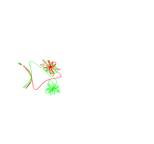
Figure 2: Seen from above are shown the numerical simulation of two trajectories of the magnetic pendulum: the attractive force between the pendulum and the fixed magnet separated by distance $r$ is taken to be proportionnal to $-\vec{r}/r^{3}$ (Coulombian-like); in addition there is the usual linear force due to gravity and directed towards the center of the triangle (the stable equilibrium point when there is no magnet) and the friction force is taken to be opposite to the speed). Starting with no initial speed from two close initial positions on the left, the two trajectories diverge one from each other very quickly (after a small fraction of second, which is the natural period of the pendulum without magnets) and end at two different equilibrium positions. The one stopping at $M_{1}$ (resp. $M_{2}$) is represented in red (resp. green) and a red (resp. green) spot indicates its starting point.

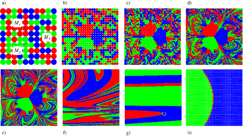
Figure 3: In a) a grid of $10\times 10$ possible initial positions is chosen and each of them is coloured according to the final position the pendulum eventually stops at (red for $M_{1}$, green for $M_{2}$, blue for $M_{3}$) with the same model as the one used to compute figure 2. In b), c), d) computations are done for a finer grid ($25\times 25$, $50\times 50$ and $100\times 100$). In e) a $500\times 500$ grid is used and the white squares indicate the portion of the picture that is zoomed on the immediate right. At very smale scales like the one in h) one can see that the borders always involve the three colours.

Unless we remain in the immediate vicinity of one of the $M$’s, it seems impossible to choose the initial conditions (position and speed) in order to make the pendulum stop at a position chosen in advance. To illustrate more quantitatively this difficulty, let us first distinguish the three magnets by a colour. Then associate one of these colours to each initial position according to the final position of the pendulum: starting above the point of Cartesian coordinates $(x,y)$ without initial speed, if the pendulum stops at $M_{1}$ (respectively $M_{2}$ or $M_{3}$) then $(x,y)$ will be coloured in red (respectively green or blue). Experimentally we can only scan a coarse-grained grid of possible initial positions (say $10\times 10$ like in figure 3a) but using a computer simulation of a more or less realistic model one can get a very high resolution pattern (figure 3e). Beyond the uniformely coloured areas surrounding $M_{1}$, $M_{2}$ and $M_{3}$, which reflect the stability of these equilibrium positions, we observe an intricate fractal-like pattern where all the three colours are intertwined at arbitrarily small scales (figures 3e-h). An infinitesimal shift from a red initial position may fall in a green area and this means that the two corresponding trajectories of the pendulum are eventually separated as far as possible one from the other (final position at $M_{2}$ instead of $M_{1}$). This is an illustration of the extreme sensitivity of the dynamics with respect to the initial conditions, or to any kind of perturbation, and this behaviour characterises what is called a chaotic system. More precisely, the linearisation $\dot{\delta\vec{r}}=A\delta\vec{r}$ of a differential equation in the neighbourhood of a given solution — where $A$ is a matrix independent of the variation $\delta\vec{r}$ but generally depends on time $t$ — leads generically to some exponential behaviour of the shift $\delta\vec{r}(t)\sim\delta\vec{r}(0)\,\mathrm{e}^{t/\tau}$ where $\tau$ is a typical time scale (known as the Lyapunov time).

Therefore, it is true that predictibility about one individual trajectory fails beyond durations of order $\tau$ : it should require an irrealistic precision on all the experimental conditions or on all the parameters of the modelisation to predict correctly the final position of the pendulum for an arbitrary set of initial conditions. This may include the gravitational perturbation due to the mass of a thundercloud moving above the place where the pendulum is and, of course, the famous flap of a butterfly wing in Brazil [7].

2 Ubiquity of chaotic behaviour

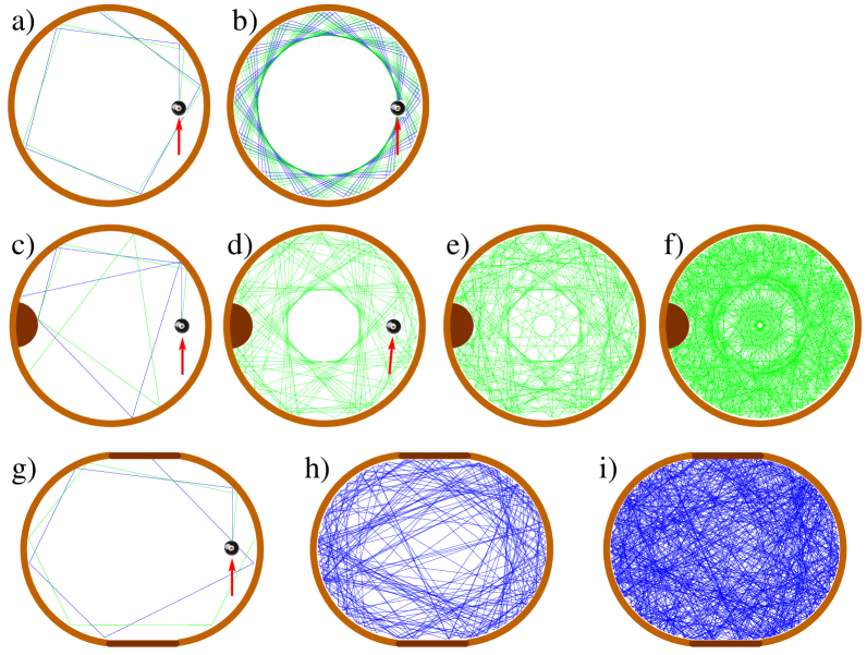
Figure 4: A ball bouncing without friction in a circular 2D-billiard has a regular motion. The difference between two different trajectories, in blue and green in a) and b), is proportional to the elapsed time, unlike in chaotic systems where this growth is exponential. The two constants of motion (energy and angular momentum) impose some selection rules that prevent most trajectories to explore the central zone of the billiard. When the rotational symmetry is broken (by a bump for the billiard in the second line or by stretching the circle into a stadium-shaped billiard in the third line), the number of constants (only the energy) becomes lower than the number of degrees of freedom (D=2) and the system becomes chaotic: as seen in c) and g) two trajectories split very quickly and, as time grows, an individual trajectory explores all the area of the billiard. From [8, figure 10.7].

As we have seen with the magnetic pendulum there is no need to consider a system as complex as the Earth atmosphere to deal with a chaotic system (by the way, Lorenz’climatic model was described by three parameters [9, eqs. (25), (26), (27)]). In fact chaos is naturally the rule and regular motion is the exception: when dissipation is negligible, for a system with $D$ degrees of freedom it would require to have $D$ independent constants of motion to keep a regular motion (such systems are called integrable because, unlike what occurs in chaotic systems, in principle the equations of motion can be solved at least locally in an appropriate coordinate system). This can be understood because the constants of motion (energy, linear momentum, angular momentum) can be seen as constraints imposing some restrictions on the dynamics: during its evolution, say, an isolated system does not explore all the possible configurations, just the ones that correspond to the same energy as the one it had initially. As soon as a constant of motion is lost, for instance, by virtue of Noether theorem, when a continuous symmetry is broken (see for instance [4, § 4]), the system becomes chaotic. The pendulum has $D=2$ degrees of freedom (say the coordinates $(x,y)$ of the projection of its position on a horizontal plane). The regularity of the frictionless simple pendulum comes from the two constants of motion: its energy (due to time-translation invariance) and its angular momentum (due to rotational invariance with respect to the vertical axis). On the contrary, even if friction were still negligeable, the magnetic pendulum would still be chaotic precisely because the external magnets break the continuous rotational invariance. Figure 4 provides another illustration of the importance of symmetries for preserving a regular motion.

Figure 5: It is the chaotic nature of the dynamics of rolling dices that make them an appropriate random generator machine.

The lost of predictatibility is therefore ubiquitous and this leads to the concepts of chance and contingency. Even if the dynamical equations are perfectly deterministic, after a characteristic time $\tau$, the system behaves as if it were “at random”, or more precisely what we call “random” or “stochastic” reveals a lost of the information that would be needed to predict the evolution of the system with no surprise. From what we have just discussed, it is therefore quite easy to get a physical random generator, even more simpler and reliable than the magnetic pendulum : a dice does the job or even the toss of a coin or a lottery ball (figure 5).

3 The stability of probabilities: the secret of the success of statistical physics

The ubiquity of chaotic systems leads to two severe issues: (i) the first concerns predictability which is one of the cornerstone of science, (ii) the second concerns objectivity since the lack of information that randomness represents depends a priori on the observer: wouldn’t a cleverer observer with more skills in modeling, more ability of computing or more memory space find less randomness in Nature? In 1814 Pierre-Simon de Laplace proposed to pursue this logic up to an idealised intelligence for whom no chance would exist [10, p. 2].

However, in practice, the exponential amplification of perturbations during the evolution of a chaotic system simplifies the situation. Dividing the initial uncertainty $\delta\vec{r}(0)$ by $10^{n}$ increases linearly with $n$, more precisely by $n\tau\ln 10$, the time $t$ when $\delta\vec{r}$ reaches a given value. So even if we take the ratio of the size of the observable universe to the radius of the proton for which $n$ is about 42, we extend the duration of reliability by less than $100\tau$ which is less than one minute for the magnetic pendulum. Therefore from a physicist point of view, the time at which a random behaviour appears is very robust and does not depend much on the experimental conditions of the observation and can be safely considered as objective. On the other hand, for times shorter than $\tau$ predictions with simple models remain reliable. The most striking example, which is of first importance not only for having contributed to the development of science but, above all, for having provided a stable enough environment for intelligent life to evolve on Earth, is provided by celestial mechanics. The two-body gravitational problem leads to the regular Keplerian ellipses which allow to reproduce the motion of the celestial bodies with a great accuracy for centuries. However, as soon as a third body is involved (not to speak of the eight main planets of the Solar System), there cannot be found enough constants of motion to get a regular motion: the discovery, by Henri Poincaré at the end of the xix${}^{\text{th}}$ Century, of what would be called chaos actually comes from his mathematical studies on the motion of three bodies interacting by gravity. As far as the Solar System is concern, $\tau$ is of order of hundreds of millions years [11] and predictability is safe at mankind scale (if we take into account the small bodies like asteroids, that is another story).

These matters of time-scales are not the end of the argument of course. One way to answer to both issues (i) and (ii) is also to consider collective effects and establish statistical laws. If the predictability of one specific event or of one trajectory may truly be challenged by a chaotic behaviour, the probability laws and some collective properties obtained by averaging on many degrees of freedom or on many observations provide reliable predictions and objective facts. The origin of this stability can be traced back to the law of large numbers: under general assumptions, the relative fluctuations within a sequence of $N$ independent events are of order $1/\sqrt{N}$. For instance, whereas we cannot predict the final position of the magnetic pendulum, we can safely say that after $N$ launching of the pendulum from various equidistributed initial positions one will obtain about $N/3$ trajectories ending on each $M$ in the equilateral configuration and this number is expected to fluctuate within a margin of order $\sqrt{N}$ as shown on the following table where the number of coloured dots is extracted from the simulations in figure 3.

Grid of initial positions	$N/3$	Red	Green	Blue
$10\times 10$	33	36	36	28
$25\times 25$	208	220	218	187
$50\times 50$	833	815	827	858
$100\times 100$	3 333	3 335	3 321	3344
$500\times 500$	83 333	83 125	82 965	83 910

A too large deviation would indicate that the configuration is biased and would indeed provide a quantitative measure of this bias.

In statistical physics $N$ is of the order of the Avogadro number $N_{A}\simeq 6\ 10^{23}$ and, then, the relative fluctuations are of order $10^{-12}$ which is usually much below what is experimentally accessible. Some quantities based on averages, like the temperature or the pressure (figure 7), are therefore very relevant for describing physical properties at macroscopic scales.

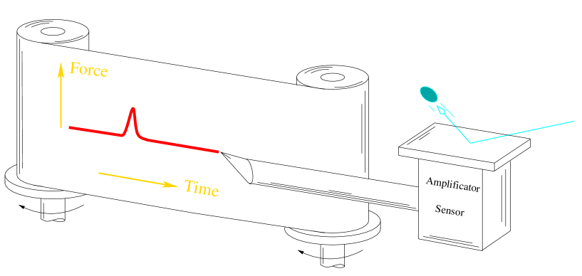
Figure 6: A schematic device that is able to measure the recoil force due to one molecule hitting a plate.

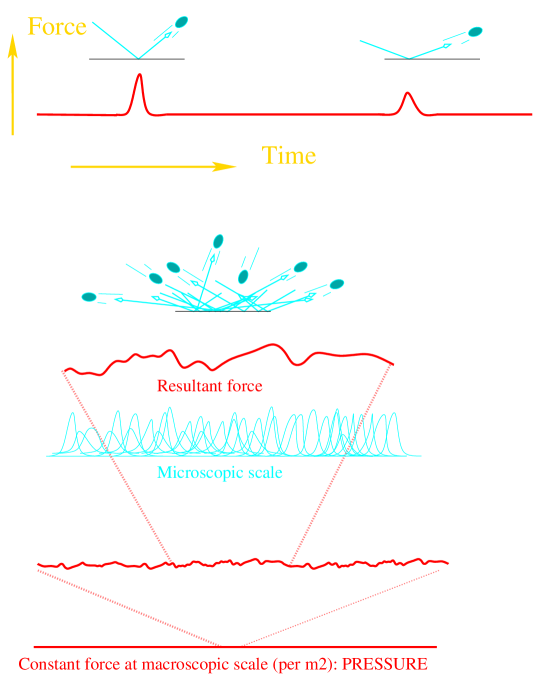
Figure 7: The device in figure 6 is used to measure the force on the plate when the number of molecules is increased. The more numerous the molecules, the more hits per unit of time and the less fluctuating the force is. At macroscopic scales, no fluctuations of the force can be detected and this constant average force per unit of surface is a stable quantity independent on the microscopic events: thus emerges the pressure.

Although they are not well-defined at microscopic scales (talking of the temperature or the pressure for one molecule is far-fetched), at larger scales such physical properties emerge from a collective effect. Although the statistical system is fully chaotic at microscopic scales, the emergent properties at macroscopic scales are insensitive to initial conditions. To comprehend a system one has to give up almost all the information concerning its huge number of parts: not only keeping this information is not feasible in practice but, above all, it would not be relevant for a global study. For instance, all the existing memory space (books, hard drive, etc.) could not register the positions and the velocities of all the molecules in one litre of air; had all these raw data be measurable and stored, they would be completely over-abundant and would require to be synthesized to know, say, if the container would resist when doubling the quantity of gas inside it. Abandoning almost all the information is not an acknowledgement of weakness in front of complexity but rather a necessity for bringing out the physical quantities that are pertinent at large scales. These emergent stable properties define most, if not all, the macroscopic objects and are involved in the physical laws governing them. Pruning the information from one level of a hierarchy of physical structures (from quarks to cosmic filaments of superclusters of galaxies, say) to the upper one helps to gain in universality. The macroscopic quantities and the laws linking them become independent of much more microscopic details than the position and the velocities of its constituants. The law of perfect gas $PV=nRT$ is independent of the nature of the constituents as long as their interactions are negligible: it remains valid for a gas made of elements as different as one simple Helium atom and a much more complex Carbon Dioxide molecule. Another exemple of emergent property is the transparency: it can be quantitatively defined for materials that, at the microscopical level, are as different as water, diamond or glass, although it is a non-sense of talking about the transparency of an individual molecule.

This is all the art of statistical physics to identify the properties that shoud be extracted from a wide collection of microscopic variables. Climbing up the probably endless hierachy of physical systems is not less difficult or fundamental than following the opposite way followed by the reductionnists.

4 A concluding historical comment

More than one hundred years ago Poincaré was aware that the extreme sensitivity to initial conditions would challenge meteorologists:

It may happen that small differences in the initial conditions produce very great ones in the final phenomena. A small error in the former will produce an enormous error in the latter. Prediction becomes impossible, and we have the fortuitous phenomenon. […]
We will borrow [an example] from meteorology. Why have meteorologists such difficulty in predicting the weather with any certainty? Why is it that showers and even storms seem to come by chance, so that many people think it quite natural to pray for rain or fine weather, though they would consider it ridiculous to ask for an eclipse by prayer? We see that great disturbances are generally produced in regions where the atmosphere is in unstable equilibrium. The meteorologists see very well that the equilibrium is unstable, that a cyclone will be formed somewhere, but exactly where they are not in a position to say ; a tenth of a degree more or less at any given point, and the cyclone will burst here and not there. [13, § II, p. 259-260]

In the communication whose title was to give birth to the notion of “butterfly effect”, it is often forgotten that, beyond the chaotic behaviour of the Earth atmophere, Lorenz was putting forward the stability of the statistics one may establish:

More generally, I am proposing that over the years minuscule disturbances neither increase nor decrease the frequency of occurrences of various weather events such as tornados; the most they may do is to modify the sequences in which they occur. [7, 1st page]

I hope the present contribution have respected Lorenz original message.

References

- [1] Y. Kosmann-Schwarzbach. The Noether theorems. Invariance and conservation laws in the twentieth century (sources and studies in the history of mathematics and physical sciences). Springer, 2010. Translated by Bertram E. Schwarzbach from the French original edition (Les Éditions de l’École Polytechnique, 2004).
- [2] M. Planck. Where is science going? Norton & Company, New York, 1932. Translation by J. Murphy from the German Vom Relativen zum Absoluten [16].
- [3] A. Einstein. Maxwell’s influence on the development of the conception of physical reality. In James Clerk Maxwell, A Commemoration Volume 1831–1931. Cambridge University Press, Cambridge, 1931, pages 66–73.
- [4] A. Mouchet. Symmetry : a bridge between nature and culture. In Emmer et al. [5], pages 235–244.
- [5] M. Emmer, M. Abate, and M. Villarreal, editors. Imagine Maths 4. Between culture and mathematics. Unione Matematica Italiana. Instituto Veneto di Scienze, Lettere ed arti, Venezia e Bologna, 2015.
- [6] W. Pagel. Joan Baptista Van Helmont: Reformer of Science and Medicine. Cambridge Monographs in the History of Medicine. Cambridge University Press, Cambridge, 1982.
- [7] E. N. Lorenz. Predictability: Does the flap of a butterfly’s wings in Brazil set off a tornado in Texas? (1972). Reproduced in [15, Appendix 1] and available at http://eaps4.mit.edu/research/Lorenz/Butterfly_1972.pdf.
- [8] A. Mouchet. L’élégante efficacité des symétries. UniverSciences. Dunod, Paris, 2013.
- [9] E. N. Lorenz. Deterministic nonperiodic flow. J. Atmospheric Sci., 20(2):pages 130–141 (1963).
- [10] P.-S. de Laplace. Essai philosophiques sur les probabilités. Courcier, Paris, 1814. English translation by F. W. Truscott and F. L. Emory A philosophical essay on probabilities, Wiley, New York 1902. Laplace’s complete works are available in French on http://gallica.bnf.fr/.
- [11] J. Laskar. Is the solar system stable? Progr. Math. Phys., 66:pages 239–270 (2013). Available online arXiv:1209.5996.
- [12] A. Mouchet. Reflections on the four facets of symmetry: how physics exemplifies rational thinking. Eur. Phys. J. H, 38:pages 661–702 (2013).
- [13] H. Poincaré. Le hasard. La Revue du Mois, 3:pages 257–276 (1907). Available in French on http://henripoincarepapers.univ-lorraine.fr/bibliohp. Reproduced as chap. IV of [14].
- [14] H. Poincaré. Science and method. Dover Publications, Inc., New York, 1959. Translated by Francis Maitland from the French Science et méthode (Flammarion, 1908).
- [15] E. N. Lorenz. The essence of chaos (Jessie and John Danz Lectures). University of Washington Press, Washington, 1993.
- [16] M. Planck. Vom relativen zum absoluten. Die Naturwissenschaften, 13(3):pages 53–59 (1925). Translated in English in [2].