What is controlling the fragmentation in the Infrared Dark Cloud G14.225–0.506?
Different level of fragmentation in twin hubs

Abstract

We present observations of the 1.3 mm continuum emission toward hub-N and hub-S of the infrared dark cloud G14.225–0.506 carried out with the Submillimeter Array, together with observations of the dust emission at 870 $\mu$m and 350 $\mu$m obtained with APEX and CSO telescopes. The large scale dust emission of both hubs consists of a single peaked clump elongated in the direction of the associated filament. At small scales, the SMA images reveal that both hubs fragment into several dust condensations. The fragmentation level was assessed under the same conditions and we found that hub-N presents 4 fragments while hub-S is more fragmented, with 13 fragments identified. We studied the density structure by means of a simultaneous fit of the radial intensity profile at 870 and 350 $\mu$m and the spectral energy distribution adopting a Plummer-like function to describe the density structure. The parameters inferred from the model are remarkably similar in both hubs, suggesting that density structure could not be responsible in determining the fragmentation level. We estimated several physical parameters such as the level of turbulence and the magnetic field strength, and we found no significant differences between these hubs. The Jeans analysis indicates that the observed fragmentation is more consistent with thermal Jeans fragmentation compared with a scenario that turbulent support is included. The lower fragmentation level observed in hub-N could be explained in terms of stronger UV radiation effects from a nearby HII region, evolutionary effects, and/or stronger magnetic fields at small scales, a scenario that should be further investigated.

1. Introduction

One ubiquitous fact in the process of formation of intermediate/high-mass stars is that they are usually found associated with clusters of lower-mass stars (e. g., Pudritz, 2002; Lada & Lada, 2003). However, the process behind the formation of such clusters is unclear as it remains ambiguous how a cloud core fragments to finally form a cluster. A common approach is to assume that the fragmentation is controlled by gravitational instability, where the velocity dispersion is, at best, accounted for only as an extra source of pressure support. In massive star-forming regions several studies show that thermal fragmentation alone does not account for the observed masses and/or core (fragment) separation (e. g., Zhang et al., 2009; Bontemps et al., 2010; Pillai et al., 2011; Wang et al., 2011; Naranjo-Romero et al., 2012; van Kempen et al., 2012; Wang et al., 2014; Zhang et al., 2015; Liu et al., 2015). Most of these works only address the formation of massive dense cores, which are far more massive than the thermal Jeans mass, and thus do not follow thermal Jeans fragmentation. However, in stellar clusters, most of stars are low-mass stars and their masses are related to thermal Jeans mass, as found by Takahashi et al. (2013), Palau et al. (2015), and Teixeira et al. (2015), raising the question of what is controlling the fragmentation process? The observational results suggest that cloud fragmentation leading to the formation of pre-stellar cores must be controlled by a complex interaction of gravitational instability, turbulence, magnetic fields, cloud rotation, and stellar feedback (e. g., Padoan & Nordlund, 2002; Hosking & Whitworth, 2004; Machida et al., 2005; Girart et al., 2013).

The infrared dark cloud (IRDC) G14.225–0.506 (hereafter G14.2), also known as M17 SWex (Povich & Whitney, 2010), is part of an extended (77 pc$\times 16$ pc) and massive ($>$10⁵ $M_{\sun}$) molecular cloud discovered by Elmegreen & Lada (1976) and located southwest of the Galactic HII region M17. The distance to M17 has been recently determined through trigonometric parallaxes of CH₃OH masers, to be 1.98${}^{+0.14}_{-0.12}$ kpc (Xu et al., 2011; Wu et al., 2014). Similar local standard of rest velocity (Elmegreen et al., 1979; Busquet et al., 2013) suggests that the bright HII region M17 and the IRDC are located at the same distance. The cloud is associated with star formation activity as revealed by the presence of several H₂O masers (Jaffe et al., 1981; Palagi et al., 1993; Wang et al., 2006) and intermediate-mass YSOs (Povich & Whitney, 2010). Through the analysis of near-/mid-infrared photometry Spitzer data, Povich & Whitney (2010) report an absence of early O stars and suggest a delay in the onset of massive star formation in the region, concluding that G14.2 represents a proto-OB association that has not yet formed its most massive stars.

Recent high angular resolution observations of the NH₃ dense gas, obtained by combining VLA and Effelsberg 100 m data (Busquet et al., 2013), reveal a network of filaments constituting two hub-filament systems. Hubs are associated with H₂O maser emission (Wang et al., 2006) and mid-infrared sources (Povich & Whitney, 2010). They appear more compact, are warmer ($T_{\mathrm{rot}}$$\sim$15 K) and show larger velocity dispersion and larger masses per unit length than filaments (Busquet et al., 2013), suggesting that they are the main sites of stellar activity within the cloud. In Figure 1 we provide a general perspective of the cloud, showing the dense filaments and hubs and their association with IR sources and/or water masers.

In this paper we present 1.3 mm observations performed with the Submillimeter Array (SMA), 870 $\mu$m observations carried out with the LABOCA bolometer at the APEX telescope, and 350 $\mu$m observations with the SHARC II bolometer at the Caltech Submillimeter Observatory (CSO), toward the two hubs, dubbed hub-N and hub-S (see Fig. 1). These observations are aimed at studying the cloud fragmentation process that leads to the formation of dense core fragments. Section 2 describes the observations and data reduction process. In Section 3 we present the results of the dust continuum emission observations, and their analysis is presented in Section 4. We discuss the interplay between density, turbulence, magnetic fields, UV radiation feedback, and evolutionary effects in the fragmentation process in Section 5. Finally, in Section 6 we list the main conclusions.

Table 1SMA observational parameters

Source	Date	Configuration	Number	Proj. baselines	Gain	Bandpass	Flux	$\nu_{\mathrm{LO}}$a	Continuum bandwidth
			of Antennas	(m)	calibrator		calibrator	(GHz)	(GHz)
Hub-S	2008/06/29	compact	8	16–139	1733$-$130/1911$-$201	3c273/3c454.3	Uranus	221.98	3.6
Hub-S	2008/07/21	extended	7	44–226	1733$-$130/1911$-$201	3c273/3c454.3	Uranus	225.42	3.4
Hub-N	2011/04/19	compact	8	16–077	1733$-$130/1924$-$292	3c454.3	Neptune	224.66	7.8
Hub-Nb	2015/04/04	extended	7	23–226	1733$-$130	3c273	Titan	225.42	7.6
Hub-N	2014/08/21	very extended	5	68–432	1733$-$130	3c279	Ceres	225.47	8.0

• Center local oscilator frequency.

• Data taken with the new correlator SWARM, although only data belonging to the old ACIS correlator are used in this work.

Table 2SMA imaging parameters

Source	Configuration	$\theta_{\mathrm{LAS}}$a	Synthesized beam	Rms noiseb
			FWHM, P. Ac
		(arcsec)	(arcsec, $\arcdeg$)	(m$\rm Jy~{}beam^{-1}$)
Hub-S	compact	7	$3\farcs 09\times 2\farcs 28$, $-$57$\arcdeg$	2.8
Hub-S	extended	3	$1\farcs 23\times 1\farcs 09$, $-5\arcdeg$	1.2
Hub-S	combined	7	$1\farcs 53\times 1\farcs 41$, $-$35$\arcdeg$	1.0
Hub-N	compact	7	$4\farcs 13\times 2\farcs 75$, $-$35$\arcdeg$	2.0
Hub-N	extended	4	$1\farcs 40\times 0\farcs 97$, $-$62$\arcdeg$	2.0
Hub-N	very extended	2	$1\farcs 57\times 0\farcs 46$, $-79\arcdeg$	3.5
Hub-N	combined	7	$1\farcs 46\times 0\farcs 46$, $-78\arcdeg$	1.0

• Largest angular structure to which an interferometer is sensitive $[\theta_{\mathrm{LAS}}/\mathrm{arcsec}]$=91.02$[u_{\rm min}/k\lambda]^{-1}$, where $u_{\rm min}$ is the shortest baseline (Palau et al., 2010).

• Root-mean-square noise level of the continuum data.

• FWHM: full-width at half-maximum; P. A.: position angle.

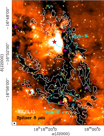
Figure 1.— Overview of the large scale structure of the G14.2 complex. White contours represent the $3\sigma$ contour level (27 m$\rm Jy~{}beam^{-1}$ km s^-1) of the NH₃ (1,1) integrated intensity map (Busquet et al., 2013). The NH₃ synthesized beam, $8\farcs 0\times 7\farcs 2$ (P. A.$=-15\arcdeg$) is shown in the bottom left corner. Color scale is the 8 $\mu$m Spitzer image. Red stars indicate IRAS sources in the field, and pink crosses mark the position of H₂O masers (Wang et al., 2006). Color stars depict the positions of the YSOs identified by Povich & Whitney (2010) where colors and symbols indicate the YSO evolutionary stage; three-point red star: Stage 0/I (dominated by infalling envelope); four-point yellow star: Stage II (optically thick circumstellar disk); five-point green star: Stage III (optically thin disk); six-point cyan star: ambiguous (see Povich et al. 2009; Povich & Whitney 2010 for further details on the YSOs classification). The SMA field of view of the two regions mosaiced, hub-N and hub-S, are indicated with the blue contour.

2. Observations and Data Reduction

2.1. Submillimeter Array Observations

The observations were carried out with the SMA (Ho et al., 2004) between 2008 and 2015 in different array configurations. Table 1 lists the observation dates, the configuration used, the number of antennas, and the projected baselines for each observing date. We performed a mosaic of 3 pointings toward hub-S and of 2 pointings toward hub-N, covering an area of $\sim 2^{\prime}\times 1^{\prime}$ and $\sim 1^{\prime}\times 1\farcm 5$, respectively (see blue contour in Fig. 1).

For hub-S, the SMA correlator covered a 2 GHz bandwidth in each of the two sidebands, which are separated by 10 GHz. Each sideband is divided into 6 blocks, and each block consists of 4 chunks, yielding 24 chunks of 104 MHz width per sideband. For both compact and extended configurations the correlator was set to the standard mode with 256 channels per chunk, providing uniform channel spacing of 0.406 MHz (or 0.52 km s^-1) per channel across the full bandwidth of 2 GHz. On the other hand, for hub-N the observations were conducted as filler projects in different runs using the 4 GHz receivers. In this case, each sideband was divided into 12 blocks with 4 chunks of 104 MHz each. The configuration of the correlator was different for each observing run. Table 1 summarizes the details of the SMA correlator, listing the local oscillator (LO) center frequency and the total bandwidth used to build the continuum.

The zenith opacity ($\tau_{\rm{225\,GHz}}$), measured with the National Radio Astronomy Observatory (NRAO) tipping radiometer located at the Caltech Submillimeter Observatory, was stable during the observations in the compact configurations, with values $\sim 0.1$-0.2, and around 0.1 during the observations in the extended and very extended configurations.

The visibility data were calibrated using the standard procedures of MIRIAD (Sault et al., 1995). Information on the calibrators used is given in Table 1. The flux calibration is estimated to be accurate within $\sim 20$ %.

The continuum was constructed from the line-free channels in the visibility domain. To produce the CLEANed single images of the two hubs, we used the tasks “invert” (option mosaic), “mossdi”, and “restor” as recommended in the MIRIAD users guide (Sault et al., 1995). The final combined images were obtained by weighting the visibilities in inverse proportion to the noise variance. We summarize the basic parameters (synthesized beam and rms noise level) of the different maps in Table 2. In this work we focus on the dust continuum emission, leaving the analysis of the molecular line emission for a forthcoming paper.

2.2. APEX Observations

Continuum observations at 870 $\mu$m were carried out using LABOCA bolometer array, installed on the Atacama Pathfinder EXperiment (APEX) telescope. The array consists of 259 channels, which are arranged in 9 concentric hexagons around the central channel. The field of view of the array is $11\farcm 4$, and the angular resolution of each beam is $18\farcs 6\pm 1^{\prime\prime}$.

The data were acquired on 2008 August 24 and 31 during the ESO program 081.C-0880A, under excellent weather conditions (zenith opacity values ranged from 0.15 to 0.24 at 870 $\mu$m). Observations were performed using a spiral raster mapping. This observing mode consists of a set of spirals with radii between $2^{\prime}$ and $3^{\prime}$ at a combination of 9 and 4 raster positions separated by $60^{\prime\prime}$ in azimuth and elevation, with an integration time of 40 seconds per spiral. This mode provides a fully sampled and homogeneously covered map in an area of $15^{\prime}\times 15^{\prime}$. The final map consisted of a mosaic of two points centered at $\alpha$(J2000)=18^h18^m17${}^{\mbox{\scriptsize{s}}}$.5, $\delta$(J2000)=$−16\arcdeg 44^{\prime}00\farcs 0$, and $\alpha$(J2000)=18^h18^m17${}^{\mbox{\scriptsize{s}}}$.5, $\delta$(J2000)=$−16\arcdeg 57^{\prime}00\farcs 0$, respectively. The total on-source integration time was $\sim 2$ hours per position. Calibration was performed using observations of Mars as well as secondary calibrators. The absolute flux calibration uncertainty is estimated to be $\sim 8$ %. The telescope pointing was checked every hour, finding a rms pointing accuracy of 2^′′. Focus settings were checked once per night and during the sunset.

We reduced the data using MiniCRUSH software package (see Kovács, 2008). The pre-processing steps consisted of flagging dead or cross-talk channels frames with too high telescope accelerations and with unsuitable mapping speed, as well as temperature drift correction using two blind bolometers. Data reduction process included flat-fielding, opacity correction, calibration, correlated noise removal (atmospheric fluctuations seen by the whole array, as well as electronic noise originated in groups of detector channels), and de-spiking. Every scan was visually inspected to identify and discard corrupted data. The final map was smoothed to a final angular resolution of $\sim 22^{\prime\prime}$, and the rms noise level achieved was 25 m$\rm Jy~{}beam^{-1}$. In this paper we focus our attention on the dust emission associated with the two hubs, hub-N and hub-S, identified using high angular resolution NH₃ data (Busquet et al., 2013). The analysis of the entire cloud will be the subject of a forthcoming paper.

Table 3Parameters of hubs from APEX-LABOCA 870 $\mu$m and CSO-SHARC II 350 $\mu$m observations

	$\alpha$(J2000.0)	$\delta$(J2000.0)	I${}_{\nu}^{\mathrm{peak}}$	Sν	Deconvolved Size		P.A.
Source	(h:m:s)	($\arcdeg$:′:′′)	($\rm Jy~{}beam^{-1}$)	(Jy)	(arcsec)	(pc)	(°)
870 $\mu$m
hub-N	18:18:12.62	$-$16:49:34.0	06.4$\pm 0.1$	024.7$\pm$2.2	57.7$\times$33.2	0.6$\times$0.3	007.2
hub-S	18:18:13.10	$-$16:57:20.3	04.5$\pm 0.1$	020.0$\pm$1.9	63.0$\times$33.4	0.6$\times$0.3	081.5
350 $\mu$m
hub-N	18:18:12.53	$-$16:49:28.2	17.0$\pm 0.2$	111.6$\pm$7.7	30.3$\times$20.7	0.3$\times$0.2	164.4
hub-S	18:18:13.06	$-$16:57:19.2	10.1$\pm 0.2$	081.3$\pm$7.5	29.9$\times$20.9	0.3$\times$0.2	071.8

2.3. CSO SHARC II 350 $\mu$m

High angular resolution continuum observations at 350 $\mu$m were carried out using the SHARC II bolometer array, installed on the Caltech Submillimeter Observatory (CSO). The array consists of 12$\times$32 pixels (approximately 85 % of these pixels work well). The simultaneous field of view provided by this array is $2\farcm 59\times 0\farcm 97$, and the diffraction limited beam size is $\sim 9^{\prime\prime}$.

The data were acquired on 2014 March 26 ($\tau_{\mbox{\scriptsize{225~{}GHz}}}$$\simeq$0.08). The telescope pointing and focusing were checked every 1.5–2.5 hours. Mars was observed for the absolute flux calibration, with a flux calibration uncertainty of $\sim 20$ %. We used the standard 10${}^{\prime}\times 10^{\prime}$ on-the-fly (OTF) box scanning pattern, centered on the two positions $\alpha$(J2000)=18${}^{\mbox{\scriptsize{h}}}$18${}^{\mbox{\scriptsize{m}}}$13${}^{\mbox{\scriptsize{s}}}$.99; $\delta$(J2000)=$-16^{\circ}$51^′00$\farcs$40, and $\alpha$(J2000)=18${}^{\mbox{\scriptsize{h}}}$18${}^{\mbox{\scriptsize{m}}}$13${}^{\mbox{\scriptsize{s}}}$.997; $\delta$(J2000)=$-16^{\circ}$59^′00$\farcs$40. The final map covered an area of $20^{\prime}\times 10^{\prime}$. The total on-source time was 30 minutes for each of these two pointings. Data calibration was performed using the CRUSH software package (Kovács 2008). The final map was smoothed to an angular resolution of $9\farcs$6 and the rms noise level achieved was $\sim 85$ mJy beam^-1.

3. Results

3.1. Dust emission at 0.1 pc scale

Figure 2 (left panel) and Fig. 3 (top panel) show the dust emission at 870 $\mu$m (blue dashed contours) and 350 $\mu$m (grey scale) obtained with the APEX and the CSO telescopes toward hub-N and hub-S, respectively. The smaller scale structure of the dust continuum emission follows the larger scale filaments seen in extinction, i. e., hub-N appears elongated in the north-south direction. Similarly, the large scale dust continuum emission of hub-S appears elongated along the east-west direction. The morphology of the dust emission resembles that of the dense gas traced by NH₃  (Busquet et al., 2013). Table 3 summarizes the main physical parameters of the dusty envelope of both hubs, listing their peak position, peak intensity, and flux density. The deconvolved size was obtained by fitting a 2-dimensional Gaussian function. The two hubs have the same size, $0.6\times 0.3$ pc at 870 $\mu$m and $0.3\times 0.2$ pc at 350 $\mu$m. Note that the peak positions at 870 and 350 $\mu$m are offset from each other by $\sim 6^{\prime\prime}$ in hub-N and $\sim 3^{\prime\prime}$ in hub-S. This is most likely due to pointing errors. Further details on the physical properties of hubs are presented in Section 4.1 where we model the radial intensity profile and the spectral energy distribution of each hub.

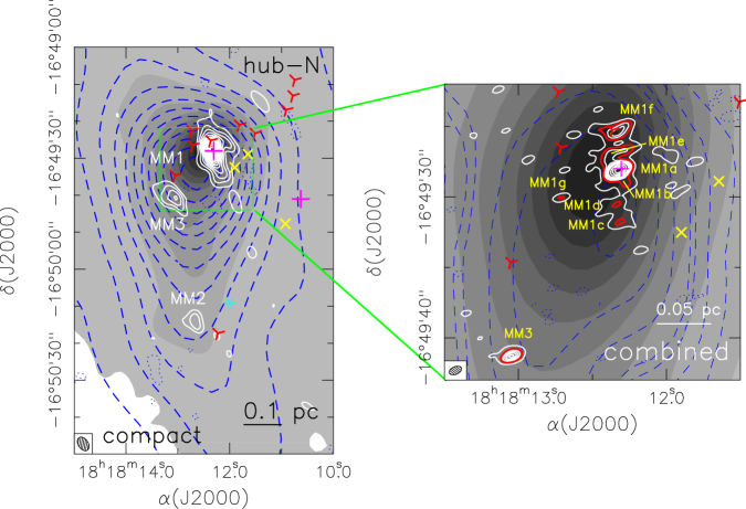
Figure 2.— Left: Contour map of the dust emission at 1.3 mm obtained with the SMA compact configuration (white contours, angular resolution $\sim$4^′′) of G14.2-hub-N overlaid on the dust emission at 350 $\mu$m from the CSO SHARC II bolometer (grey scale) and at 870 $\mu$m from LABOCA bolometer at the APEX telescope (dashed contours). Contours at 1.3 mm start at $3\sigma$ and increase in steps of $3\sigma$, where $\sigma$ is the rms of the map listed in Table 1. Blue dotted contour corresponds to the $-3\sigma$ contour level. The dashed contours at 870 $\mu$m start at $3\sigma$ rms level and increase in steps of $20\sigma$, where $\sigma$ is 25 m$\rm Jy~{}beam^{-1}$. The CSO 350 $\mu$m grey-scale image start at 2 % of the maximum, with levels increasing in 10 % of the maximum value. The synthesized beam of the SMA image is shown in the bottom left corner of the image. Right: Close-up of the MM1 and MM3 millimeter sources that show the SMA 1.3 mm continuum emission obtained by combining all configurations. The red thick contour level denotes the 6 $\sigma$ level used to identify the continuum sources. Contours range from 3 to $21\sigma$ in steps of $3\sigma$, and from 21 to $51\sigma$ in steps of $10\sigma$, where $\sigma$ is the rms of the map listed in Table 1. Dashed contours represent the NH₃ (1,1) integrated intensity emission (Busquet et al., 2013) and the grey scale is the 350 $\mu$m  image. The synthesized beam ($1\farcs 43\times 0\farcs 80$, P. A.$=-54\arcdeg$) is shown in the bottom left corner of the image. Symbols are the same as in Fig. 1.

3.2. Dust emission at 0.03 pc scale

In this section we present first the results obtained with the SMA in the compact configuration with an angular resolution of $\sim 3^{\prime\prime}-4^{\prime\prime}$, corresponding to $\sim 0.03$ pc at the distance of the source. Then, in Sect. 3.3 we show the images of each hub obtained by combining all configurations. This allows us to obtain high angular resolution maps ($\sim 1\farcs 5$) at the best possible sensitivity. From these maps, we used a $6\sigma$ threshold to identify the millimeter condensations in each hub, with $\sigma$ being the rms noise level and requesting that the 6$\sigma$ contour level is closed.

Figure 2 (left panel) and Fig. 3 (top panel) present the SMA 1.3 mm continuum emission (in white contours) obtained with the compact configuration toward hub-N and hub-S, respectively. At a similar angular resolution and similar sensitivity, 2-3 m$\rm Jy~{}beam^{-1}$, the dust envelopes of both hubs appear fragmented into dust cores. We detected 3 and 7 compact continuum condensations above a $6\sigma$ contour level toward hub-N and hub-S, respectively, in the compact configuration.

In hub-N, most of the 1.3 mm emission arise from a bright source, MM1, located at the peak of the single-dish submillimeter dust emission. This appears to be elongated along the north-south direction with a position angle of $7\arcdeg$, similar to the large scale 870 $\mu$m emission (see Table 3). There are two faint and more flattened millimeter condensations associated with hub-N: MM2 located about $46^{\prime\prime}$ south of MM1, and MM3 located $\sim 12^{\prime\prime}$ south-east of MM1. All millimeter condensations in hub-N are deeply embedded within the dust envelope and the NH₃ (1,1) dense gas emission.

The 1.3 mm SMA continuum emission of hub-S consists of 7 continuum condensations, 4 of them clustered around the peak position of the large scale envelope, forming a snake-shape structure of about $25^{\prime\prime}$ (Fig. 3-top panel). From west to east the millimeter condensations are labeled as MM2, MM3, MM4, and MM5.

3.3. Dust emission at 0.01 pc scale

The higher angular resolution images ($\sim 1\farcs 5$) reveal that both hubs fragment further. The resulting 1.3 mm continuum maps are presented in Fig. 2 (right panel) and Fig. 3 (bottom panel), which were obtained using all available SMA configurations. The sensitivity of the final SMA images is the same: 1 m$\rm Jy~{}beam^{-1}$. At a $6\sigma$ level, this sensitivity corresponds to a mass sensitivity of 0.7 $M_{\sun}$, assuming a dust temperature of 17 K (see below), a gas-to-dust mass ratio of 100, and a dust mass opacity coefficient at 1.3 mm per unit mass density of dust and unit length of 0.899 cm^-2 g^-1, which corresponds to coagulated grains with thin ice mantles in cores of densities $\sim 10^{6}$ cm^-3 (Ossenkopf & Henning, 1994). We then identified sources having peak fluxes above the $6\sigma$ rms noise level. The number of millimeter continuum condensations in hub-N is 9 while in hub-S the number of millimeter condensations is 17. In Table 4 we report the identified condensations for each hub, listing their position, peak flux, total flux density, and deconvolved size obtained for a 2-dimensional Gaussian fitting, when possible. For those sources that cannot be fitted with a Gaussian function we estimated the flux density by integrating the emission above the 4$\sigma$ level. We additionally report the association of a dust millimeter source with a near-IR source, and the presence of infrared excess at 4.5 $\mu$m according to the catalog of Povich & Whitney (2010), as well as its association with H₂O maser emission (Wang et al., 2006).

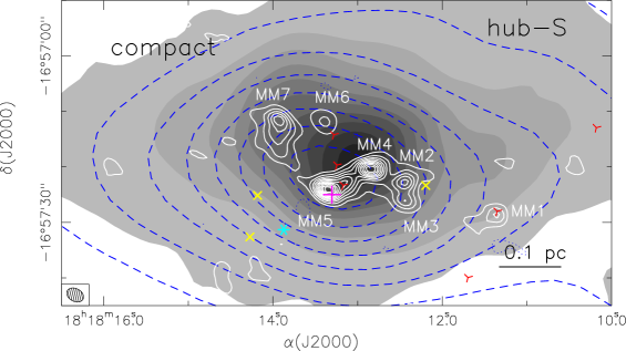
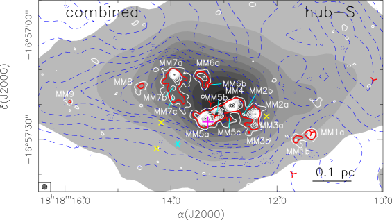
Figure 3.— Top: Same as Fig. 2 but for G14.2-hub-S. Contours at 1.3 mm start at 3$\sigma$ and increase in steps of 3$\sigma$, where $\sigma$ is the rms of the map listed in Table 1. Bottom: Contour map of the SMA dust emission at 1.3 mm toward G14.2-hub-S obtained by combining the compact and extended configuration observations (angular resolution $\simeq 1\farcs 5$) overlaid on the dust emission at 350 $\mu$m from the CSO SHARC II bolometer (grey scale) and the NH₃ (1,1) integrated intensity map (dashed contours) from Busquet et al. (2013). Contours at 1.3 mm range from 3 to $30\sigma$ increasing in steps of $3\sigma$, and from 30 to $60\sigma$ in steps of $10\sigma$, where $\sigma$ is the rms of the map listed in Table 1. Blue dotted contour corresponds to the $-3\sigma$ contour level. The red thick contour level denotes the $6\sigma$ level used to identify the continuum sources. The SMA synthesized beam is shown in the bottom left corner of each image. Symbols are the same as in Fig. 1.

As can be seen in the close-up image of hub-N (Fig. 2-right panel) the high angular resolution map shows that in addition to MM2 and MM3, the strongest millimeter continuum source MM1, which has a peak intensity of 56 m$\rm Jy~{}beam^{-1}$, breaks up in 6 additional sources. The strongest source MM1a is associated with a H₂O maser spot (Wang et al., 2006). There are two sources located north of MM1a, labelled as MM1e and MM1f, and three faint sources south of MM1a, labelled as MM1b, MM1c, and MM1d. MM1f is associated with a YSO, identified in the Spitzer image by Povich & Whitney (2010), in Stage 0/I of evolution, which means it is dominated by an infalling envelope. Moreover, this source presents a 4.5 $\mu$m excess (Povich & Whitney, 2010). Sources with this feature are typically called “Extended Green Objects” (EGOs) and is due to protostellar outflow activity, indicating that MM1f could be a massive YSO candidate (Cyganowski et al., 2008). We detected an additional source, called MM1g, which lies about $5\farcs 6$ south east of MM1a whose emission is very compact and faint. While MM3 is still detected in the high-angular resolution map, the emission of MM2, detected only at a $4\sigma$ level, is filtered out due to a combination of a faint and flattened structure.

Regarding the high angular resolution 1.3 mm image of hub-S, Fig. 3 (bottom panel) shows that the snake-shape structure located at the center of the image, which consisted in 4 fragments in the compact configuration, breaks up into 7 condensations. The strongest and compact source MM5a is associated with a H₂O maser (Wang et al., 2006) and MM5b has its peak position very close to a YSO in the Stage 0/I of evolution that presents an excess in the 4.5 $\mu$m  Spitzer band. MM1a and MM1b lie at the border of the dust envelope, about $15^{\prime\prime}$ to the west of MM5a. The brightest source, MM1a, is associated with an infrared source classified by Povich & Whitney (2010) as a YSO in the Stage 0/I of evolution (i. e., dominated by an infalling envelope). MM6 splits in two sources separated $2\farcs 2$, and MM7 breaks up in three sources, MM7a is the strongest one, and MM7b and MM7c are $3^{\prime\prime}$ and $6^{\prime\prime}$ to the south, respectively. The higher sensitivity of the combined map allowed to detect two additional sources, MM8 and MM9, with a high-enough signal-to-noise ratio.

Assuming that the dust emission at 1.3 mm is optically thin and that the temperature distribution is uniform, we estimated the mass of each millimeter condensation adopting a gas-to-dust ratio of 100 and using the dust mass opacity coefficient at 1.3 mm per unit mass density of dust and unit length of 0.899 cm² g^-1 (Ossenkopf & Henning, 1994). In both hubs, the rotational temperature obtained from NH₃ observations is 15 K (Busquet et al., 2013). We converted $T_{\mathrm{rot}}$ to gas kinetic temperature using the expression provided by Tafalla et al. (2004), and obtained $T_{\mathrm{kin}}$$\simeq$17 K. Assuming $T_{\mathrm{kin}}$=$T_{\mathrm{d}}$ the masses of the continuum sources are estimated to be in the range $1-13$ $M_{\sun}$ in hub-N and $0.7-18$ $M_{\sun}$ in hub-S. We report the mass of each millimeter condensation in Table 4. Due to the uncertainty in the dust mass opacity coefficient, the values of the derived masses are good to within a factor of 2. While in hub-N only MM1a has a mass larger than 10 $M_{\sun}$, in hub-S there are four sources with $M>10$ $M_{\sun}$. The sum of all mass estimated from the 1.3 mm dust continuum emission is 34.2 $M_{\sun}$ and 95.1 $M_{\sun}$ in hub-N and hub-S, respectively. It is worth noting that the mass of all millimeter condensations, except for MM2 in hub-N, have been measured using the combined image.

Table 4SMA 1.3 mm continuum sources for the two hubs

Source_ID	Positiona		I${}_{\nu}^{\mathrm{peak}}$	Sν	Deconvolved Size		P.A.	$M_{\rm{H_{2}}}$	near-IRb	H2O c	4.5 $\mu$m b
	$\alpha$(J2000.0)	$\delta$(J2000.0)	(m$\rm Jy~{}beam^{-1}$)	(mJy)	(arcsec)	(AU$\times$AU)	(°)	($M_{\sun}$)	source?	maser?	excess?
Hub-N
MM1a	18:18:12.32	$-$16:49:28.1	56.4$\pm$0.9	118.3$\pm$2.7	0.8$\times$0.7	1630$\times$1380	099	13.0	…	$\surd$	…
MM1be	18:18:12.30	$-$16:49:28.7	09.2$\pm$0.2	009.6$\pm$0.8	…	$<2890$	…	01.1	…	…	…
MM1ce	18:18:12.32	$-$16:49:31.9	06.6$\pm$0.4	010.0$\pm$2.5	…	$<2890$	…	01.1	…	…	…
MM1de	18:18:12.33	$-$16:49:30.5	06.7$\pm$0.5	010.1$\pm$1.8	…	$<2890$	…	01.1	…	…	…
MM1ee	18:18:12.37	$-$16:49:26.9	11.0$\pm$1.2	025.2$\pm$0.7	…	$<2890$	…	02.8	…	…	…
MM1f	18:18:12.33	$-$16:49:25.3	14.0$\pm$0.8	059.2$\pm 4.5$	2.5$\times$0.8	4950$\times$1650	111	06.5	$\surd$…	$\surd$
MM1g	18:18:12.71	$-$16:49:30.1	06.4$\pm$0.9	009.2$\pm$0.3	0.8$\times$0.3	1630$\times$0510	083	01.0	…	…	…
MM2d	18:18:12.67	$-$16:50:14.3	16.9$\pm$2.2	033.1$\pm$6.3	4.1$\times$2.6	8120$\times$5150	068	03.6	…	…	…
MM3	18:18:13.05	$-$16:49:41.3	18.1$\pm$0.9	036.2$\pm$2.6	0.9$\times$0.6	1780$\times$1190	097	04.0	…	…	…
Hub-S
MM1a	18:18:11.36	$-$16:57:28.6	17.4$\pm$0.2	044.3$\pm$0.8	2.0$\times$1.7	3920$\times$3360	119	04.9	$\surd$	…	…
MM1b	18:18:11.61	$-$16:57:29.8	08.6$\pm$0.2	028.9$\pm$0.9	2.9$\times$1.6	5760$\times$3170	103	03.2	…	…	…
MM2	18:18:12.43	$-$16:57:22.6	23.1$\pm$0.3	083.3$\pm$1.0	2.5$\times$2.2	4960$\times$4360	117	09.2	…	…	…
MM2be	18:18:12.63	$-$16:57:22.8	09.6$\pm$0.3	008.8$\pm$1.7	…	$<2800$	…	01.0	…	…	…
MM3a	18:18:12.42	$-$16:57:25.7	12.4$\pm$0.2	048.9$\pm$1.1	2.3$\times$2.0	4550$\times$3960	168	05.4	…	…	…
MM3be	18:18:12.52	$-$16:57:27.9	06.3$\pm$0.2	006.2$\pm$1.5	…	$<2800$	…	00.7	…	…	…
MM4	18:18:12.84	$-$16:57:20.3	43.6$\pm$0.2	136.6$\pm$0.9	2.8$\times$1.5	5600$\times$2970	111	15.1	…	…	…
MM5a	18:18:13.34	$-$16:57:24.1	56.1$\pm$0.2	161.2$\pm$0.8	2.2$\times$1.8	4430$\times$3530	093	17.8	…	$\surd$	…
MM5b	18:18:13.15	$-$16:57:22.8	26.2$\pm$0.3	105.2$\pm$1.1	3.4$\times$1.8	6670$\times$3600	148	11.6	$\surd$	…	$\surd$
MM5ce	18:18:12.90	$-$16:57:24.0	07.9$\pm$0.4	007.6$\pm$0.5	…	$<2800$	…	00.8	…	…	…
MM6a	18:18:13.40	$-$16:57:12.2	11.3$\pm$0.3	059.9$\pm$1.4	3.5$\times$2.6	6940$\times$5240	029	06.6	…	…	…
MM6be	18:18:13.38	$-$16:57:14.4	07.3$\pm$0.5	006.6$\pm$0.8	…	$<2800$	…	00.7	…	…	…
MM7a	18:18:13.92	$-$16:57:11.7	25.6$\pm$0.2	094.3$\pm$1.1	2.9$\times$1.9	5750$\times$3880	028	10.4	…	…	…
MM7be	18:18:13.95	$-$16:57:15.0	10.1$\pm$0.7	019.5$\pm$1.2	…	$<2800$	…	02.1	…	…	…
MM7ce	18:18:13.97	$-$16:57:18.0	09.9$\pm$1.8	014.9$\pm$1.5	…	$<2800$	…	01.6	…	…	…
MM8	18:18:14.86	$-$16:57:14.9	07.3$\pm$0.2	025.8$\pm$1.0	2.9$\times$1.8	5870$\times$3490	131	02.8	…	…	…
MM9	18:18:15.93	$-$16:57:19.2	05.8$\pm$0.3	011.3$\pm$0.6	2.0$\times$0.9	3930$\times$1750	060	01.2	…	…	…

• Source positions determined from a 2D Gaussian fit. Units of R. A in (h:m:s) and Decl. in ($\arcdeg$:^′:^′′).

• near-IR source or 4.5 $\mu$m Spitzer excess reported by Povich & Whitney (2010).

• H₂O maser detected (Wang et al., 2006).

• Properties of MM2 determined using the SMA image at $4^{\prime\prime}$ resolution.

• A 2D gaussian cannot be fitted and the peak intensity and total flux density were obtained by integrating the emission within the 4$\sigma$ contour level.

3.4. Fragmentation level

In the previous sections we have shown the SMA maps at different resolutions. Now, the aim is to estimate the fragmentation level in each hub. To do so, we need first to obtain images with the same angular resolution to be easily comparable. We then performed the imaging of each hub using a common $uv$-range of visibilities (8-160 k$\lambda$). The observations of hub-N have more visibilities at longer $uv$-distances than hub-S, which results in a slightly smaller beam, especially in one direction (roughly the north-south direction), so we convolved the map to the beam obtained for hub-S (i. e., $1\farcs 53\times 1\farcs 41$). In addition, since our SMA observations consist of a small mosaic instead of a single pointing, and the total field of view of each hub is different, we need to define a region in which we can evaluate in a consistent way the fragmentation level in each hub. The typical radii of compact and embedded clusters and subclusters lie in the range $0.1-0.2$ pc (e. g., Testi et al., 1999; Alexander & Kobulnicky, 2012; Kuhn et al., 2014). Then, we defined a radius of 0.15 pc, which corresponds to a region of $\sim 30^{\prime\prime}$ at the distance of the source. In Fig. 4 we present the 1.3 mm continuum emission in a field of view of 30^′′ for hub-N (left panel) and hub-S (right panel). Adopting this field of view and the $6\sigma$ detection threshold, we found 4 fragments in hub-N and 13 fragments in hub-S. These values are listed in Table 6. Therefore, using the proper comparison we still clearly see that hub-S has a higher fragmentation level than hub-N.

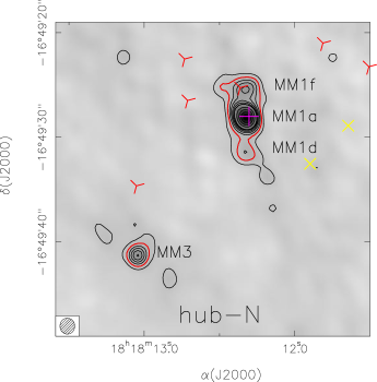
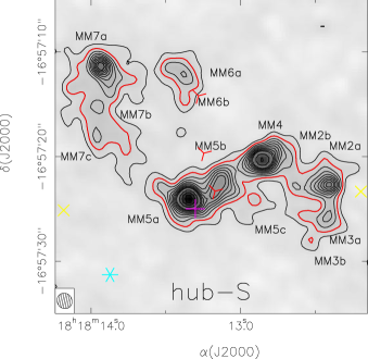
Figure 4.— Contour map of the SMA dust emission at 1.3 mm toward hub-N (left) and hub-S (right) showing a field of view of $\sim 30"\sim 0.3$ pc. Note that for hubN the combined map has been convolved to the same beam as the hub-S image for an easy comparison of the fragmentation level in each hub. The synthesized beam, $1\farcs 53\times 1\farcs 41$, is shown in the bottom left corner of each image. Contours and symbols are the same as in Fig. 2 and Fig. 3. The 6$\sigma$ rms level is indicated by the red thick contour.

4. Analysis

4.1. Radial Intensity Profiles

Recently, Palau et al. (2014) studied the relation between the fragmentation level and the density structure in a sample of 19 massive dense cores selected to be in a similar evolutionary stage, i. e., all regions harbor intermediate/high-mass protostars deeply embedded in massive dense cores that have not yet developed an ultra-compact HII region, hence comparable to our targets hub-N and hub-S. They find a weak (inverse) trend of fragmentation level and density power-law index, with steeper density profiles tending to show lower fragmentation and vice-versa. One of the main results of this work is that, within a given radius, the fragmentation level increases with average density as a combination of flat density profile and high central density. A comparison with magnetohydrodynamic simulations (Commerçon et al., 2011) suggests that the cores showing no fragmentation could be related with a strong magnetic field. In a follow-up work using the same sample of massive dense cores, Palau et al. (2015) analyze whether the fragmentation level can be explained by turbulent or thermal support, and conclude that the observed fragmentation level is more consistent with pure thermal Jeans fragmentation than fragmentation including turbulent support.

In order to investigate whether the differences of the fragmentation level in hub-N and hub-S could be explained in terms of the density structure of the envelope, we applied the model presented in Palau et al. (2014) to fit simultaneously the radial intensity profile at 870 $\mu$m and 350 $\mu$m and the spectral energy distribution (SED) assuming spherical symmetry. It is important to mention that both hubs are embedded in filamentary structures, and thus the radial profile along the filament’s main axis has contributions from the filament and the hub. Since we are interested in modelling the structure of the hub, not the filament, we extracted the radial profiles in the direction perpendicular to the filament main axis to avoid contamination from the filament itself at large distances. The radial intensity profiles at 870 $\mu$m and 350 $\mu$m were obtained in rings of 10^′′ and 6^′′ width, respectively, as a function of the projected distance from the clump center. The radial intensity profiles of hub-N and hub-S at 870 $\mu$m and 350 $\mu$m are presented in Fig. 5.

The SED of each hub was built considering the flux density at 350 and 870 $\mu$m from this work, and the flux densities measured by the ESA Herschel Space Observatory (Pilbratt et al., 2010) in the framework of the Herschel infrared Galactic Plane Survey (Hi-GAL) project, which performed an unbiased photometric survey of the Galactic plane in five photometric bands: 70, 160, 250, 350, and 500 $\mu$m (Molinari et al., 2010b). The Herschel fluxes have been measured following the standard procedures described in the Hi-GAL articles (Molinari et al., 2010a; Elia et al., 2013) using CuTEx (Molinari et al., 2011) by means of a 2-D Gaussian fit of the source brightness profile independently at each band. The fluxes at 870 $\mu$m and 350 $\mu$m obtained with the APEX and CSO telescopes, respectively, were estimated within a radius of 22^′′ and 10^′′, respectively. At 350 $\mu$m we used both the Herschel and the CSO values.

In the present model, we describe the density structure using a Plummer-like function of the form

$$\rho(r)=\rho_{c}\left[1+\left(\frac{r}{r_{c}}\right)^{2}\right]^{-p/2}$$ (1)

where $\rho_{c}$ is the central density, $r_{c}$ is the radius of the flat inner region, and $p$ is the asymptotic power index.

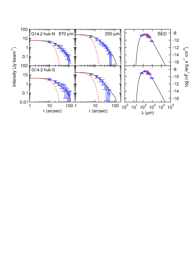
Figure 5.— Best fits for hub-N (top panels) and hub-S (bottom panels). The left and middle panels show the radial intensity profiles at 870 and 350 $\mu$m. Open blue circles with error bars show the data, the solid black line shows the best-fit model, and the dashed red line shows the beam profile. The right panel shows the spectral energy distribution. Blue open circles with error bars show the observed fluxes, and the open red circles show the model values integrated for the same aperture than the observation. The continuous black line is the SED integrated up to the model envelope radius $r_{\mathrm{max}}$ (see Table 5). Note that SHARC II and LABOCA cannot detect structures $>1^{\prime}$ scale.

The temperature was assumed to be a power-law of radius

$$T=T_{0}\Big{(}\frac{r}{r_{0}}\Big{)}^{-q},$$ (2)

where $q=2/(4+\beta)$. We assumed a dust opacity law as a power-law of frequency with index $\beta$, $\kappa_{\nu}=\kappa_{0}(\nu/\nu_{0})^{\beta}$, where $\nu_{0}$ is an arbitrary reference frequency. At $\nu_{0}=230$ GHz, we used the dust mass opacity coefficient adopted in Sect. 3.3.

We adopted a constant temperature of 8 K for radii larger than the radius where the temperature distribution of index $-q$ drops to 8 K. We stress that a minimum temperature of 10 K does not alter the results. Concerning the density distribution, we adopted, as a maximum radius of the envelope, the radius for which the envelope density achieved a value comparable to that of the ambient gas of the intecore medium, taken to be $5\times 10^{3}$ cm^-3, the same value adopted in Palau et al. (2014).

The model has five free parameters: the dust emissivity index $\beta$, the envelope temperature $T_{0}$ at the reference radius $r_{0}$, the envelope density $\rho_{0}$ extrapolated to the reference radius $r_{0}$, the radius of the inner region where density is flat (in units of $r_{0}$) $r_{c}/{r_{0}}$, and the density power law index $p$. The reference radius $r_{0}$ is arbitrary and has been taken as $r_{0}=1000$ AU. It is important to remark that $\rho_{0}$ is not the actual density at $r_{0}$, but the value given by the asymptotic density power law, $\rho_{0}=\rho_{c}(r_{0}/r_{c})^{-p}$. In fact, if $r_{0}<r_{c}$, the density $\rho_{0}$ is higher than the maximum density $\rho_{c}$. Only in the case $r_{0}\gg r_{c}$ does the density $\rho_{0}$ correspond to the actual density at $r=r_{0}$.

We used this model to fit simultaneously the observed radial intensity profiles at 870 $\mu$m and 350 $\mu$m  and the observed SED. We adopted an uncertainty in the radial intensity profiles at both 870 and 350 $\mu$m of 20 %. The uncertainty of the flux densities used in the SED was 20 % at all wavelengths, plus an additional 20 %, added quadratically, for the 70 and 160 $\mu$m values (the PACS data). Note that SHARC II and LABOCA instruments cannot detect structures larger than $1^{\prime}$ scale.

For each set of model parameters we computed the intensity map at 870 $\mu$m and 350 $\mu$m  and convolved it with a Gaussian of the size of the beam of the telescope used in the observation. The intensity profile was obtained from the convolved map, and compared with the circularly averaged observed radial intensity profiles. On the other hand, in order to compare the model with the observed SED, we computed the model flux density by integration of the model intensity profile within the aperture used to estimate the flux for each data point.

The initial search ranges for the 5 parameters were $\beta=1.5\pm 1.5$, $T_{0}=300\pm 300$ K, $\rho_{0}=(4.0\pm 4.0)\times 10^{-16}$ g cm^-3, $r_{c}/r_{0}=20\pm 20$, and $p=1.5\pm 1$. The search was carried out for 13 loops, each loop consisting in 4000 samples of the parameter space, with a search range reduced a factor 0.75 around the best-fit value of the parameters found for the last loop. A second search was performed with the best values found in the first run as starting values of the fit parameters. For this second run the initial search ranges were $0.2$, $20$ K, $2.0\times 10^{-16}$ g cm^-3, $8$, and $0.15$, for $\beta$, $T_{0}$, $\rho_{0}$, $r_{c}/r_{0}$, and $p$, respectively, and the search range was reduced a factor 0.8 for each loop. We refer to the work of Palau et al. (2014) for further details on the model and the fitting procedure used to find the best-fit model (see also Estalella et al., 2012; Sánchez-Monge et al., 2013, for details on the $\chi^{2}$ minimization).

Table 5Best-fit parameters to the radial intensity profiles and SED

		$T_{0}$a	$\rho_{0}$a				$\rho_{c}$b		$r_{\mathrm{8K}}$b	$r_{\mathrm{max}}$b
Source	$\beta$a	(K)	(g cm-3)	$r_{c}/r_{0}$a	$p$a	$\chi_{r}$a	(g cm-3)	$q$b	(pc)	(pc)
hub-N	$1.81\pm 0.08$	$51\pm 2$	$(1.3\pm 0.2)\times 10^{-15}$	$21\pm 4$	$2.24\pm 0.04$	0.69	$(1.4\pm 0.6)\times 10^{-18}$	0.34	1.05	0.62
hub-S	$1.89\pm 0.08$	$45\pm 2$	$(1.0\pm 0.2)\times 10^{-15}$	$20\pm 3$	$2.24\pm 0.04$	0.76	$(1.2\pm 0.5)\times 10^{-18}$	0.34	0.79	0.57

• Free parameter fitted by the model: $\beta$ is the dust emissivity index; $T_{0}$ and $\rho_{0}$ are the temperature and density at the reference radius $r_{0}=1000$ AU; $r_{c}/r_{0}$ is the radius of the flat inner region in units of $r_{0}$; $p$ is the asymptotic power index; $\chi_{r}$ is the reduced chi-square, $[\chi^{2}_{\mathrm{min}}/(n-5)]^{1/2}$.

• Parameters derived from the modeling: $\rho_{c}$ is the central density, $\rho_{c}=\rho_{0}(r_{c}/r_{0})^{-p}$; $q$ is the temperature power-law index; $r_{\rm{8K}}$ is the radius of the clump where the temperature drops to 8 K; $r_{\rm{max}}$ is the radius at the assumed ambient density of $5\times 10^{3}$ g cm^-3.

Figure 5 shows the best fit to the 870 and 350 $\mu$m radial intensity profile and the SED for hub-N (top panel) and hub-S (bottom panel). The fitted parameters are reported in Table 5. Interestingly, despite the fragmentation level being significantly higher in hub-S than in hub-N, Table 5 shows that the parameters inferred from the model are remarkably similar. The dust emissivity index is $\sim 1.8$–1.9, which corresponds to a temperature power law index of $q\simeq 0.34$, consistent with internal heating. The fitted temperature at 1000 AU is 51$\pm 2$ K and 45$\pm 2$ K in hub-N and hub-S, respectively. The central density, $\rho_{c}$, is (1.0–1.3)$\times 10^{-18}$ g cm^-3 and the radius of the flat inner region is $r_{c}\simeq 0.1$ pc. In Table 5 we also show the radius where the density reaches $5\times 10^{3}$  cm^-3 and the radius where the temperature drops down to 8 K. In both hubs we obtained the same index $p\simeq 2.2$ of the asymptotic density power law.

4.2. General properties of the hubs

Once we obtained the best-fit model, we derived different physical quantities, which are reported in Table 6. We estimated the total mass of each hub by integrating the model intensity up to the radius where the density profile could be measured. Within the errors, the mass of both hubs is essentially the same, being slightly more massive hub-N than hub-S. Given that we evaluated the fragmentation level within a region of 0.15 pc in radius, we estimated the mass ($M_{\rm{0.15\,pc}}$), average density ($n_{\rm{0.15\,pc}}$), and average temperature ($T_{\rm{0.15\,pc}}$) within a radius of 0.15 pc. As expected, the inferred values in both hubs are remarkably similar. Note that $T_{\rm{0.15\,pc}}$ is 18 K and 16 K in hub-N and hub-S, respectively, which is consistent with the kinetic temperature, $T_{\mathrm{kin}}$=17 K, derived using the NH₃ data (Busquet et al., 2013).

Table 6Properties of the two Hubs

			$M_{\rm{tot}}$c	$L_{\mathrm{bol}}$c	$M_{\rm{0.15\,pc}}$c	$n_{\rm{0.15\,pc}}$c	$T_{\rm{0.15\,pc}}$c	$M_{\rm{Jeans}}^{\rm{th}}$d	$\sigma_{\rm{1D,nth}}$e	$M_{\rm{Jeans}}^{\rm{tot}}$d
Source	$N_{\rm{mm}}$a	$N_{\rm{IR}}/N_{\rm{mm}}$b	($M_{\sun}$)	($L_{\sun}$)	($M_{\sun}$)	($\times 10^{5}$ cm-3)	(K)	($M_{\sun}$)	(km s-1)	($M_{\sun}$)	$\mathcal{M}$f	$\mathcal{M}_{\rm{A}}$f	$\lambda$f	$\beta_{\rm{rot}}$f
hub-N	04	1.7	$979\pm 329$	995	126	1.3	18	1.33	0.83	70	5.6	0.4	0.9	0.016
hub-S	13	0.4	$717\pm 250$	531	105	1.1	16	1.21	0.88	90	6.4	0.3	0.5	0.015

• $N_{\rm{mm}}$ is the number of fragments obtained within a field of view of 0.3 pc of diameter (see Section 3.4).

• Ratio between the number of IR sources without a millimeter counterpart within $\sim 0.3$ pc, obtained from the catalog of Povich & Whitney (2010), over the number of millimeter sources detected in this work.

• Parameters inferred from the modeling. $M_{\rm{tot}}$ is the mass computed from the model by integrating up to the radius where the density profile could be measured; $L_{\mathrm{bol}}$ is the bolometric luminosity obtained by integration of the SED; $M_{\rm{0.15\,pc}}$, $n_{\rm{0.15\,pc}}$, and $T_{\rm{0.15\,pc}}$ are the mass, average density, and average temperature within a radius of 0.15 pc.

• $M_{\rm{Jeans}}^{\rm{th}}$ is the thermal Jeans mass for the temperature $T_{\rm{0.15\,pc}}$ and density $n_{\rm{0.15\,pc}}$ (Eq. 6 of Palau et al. 2015); $M_{\rm{Jeans}}^{\rm{tot}}$ is the total Jeans mass using the total (thermal + non-thermal) velocity dispersion (Eq. 4 of Palau et al. 2015).

• $\sigma_{\rm{1D,nth}}$ is the non-thermal turbulent component of the velocity dispersion estimated as $\sigma_{\rm{1D,nth}}=\sqrt{\sigma_{\rm{obs}}^{2}-\sigma_{\rm{th}}^{2}}$ using the NH₃ (1,1) data.

• $\mathcal{M}$ is the Mach number defined as $\sigma_{\mathrm{3D,nth}}/c_{\mathrm{s}}$ where $\sigma_{\mathrm{3D,nth}}=\sqrt{3}\,\sigma_{\mathrm{1D,nth}}$; $\mathcal{M}_{\rm{A}}$ is the Alfv n Mach number, expressed as $\sqrt{3}\sigma_{\mathrm{1D,nth}}/v_{A}$ where $v_{A}=B_{\mathrm{{tot}}}/\sqrt{4\pi\rho}$ is the Alfv n speed; $\lambda=(M/\Phi_{\rm{B}})/(M/\Phi_{\rm{B}})_{\rm{cr}}$ is the mass-to-magnetic-flux ratio; and $\beta_{\rm{rot}}$ is the rotational-to-gravitational energy ratio as defined in Chen et al. (2012) and derived using NH₃ (1,1) data.

Given that our aim is to investigate the interplay between the different physical agents acting during the fragmentation process, in the following we estimated some relevant physical quantities to evaluate the relative importance of the different forces within a region of 0.3 pc in diameter, the region where we assessed the fragmentation level in each hub.

Velocity dispersion. We extracted the averaged NH₃ (1,1) spectrum of both hubs and fitted the hyperfine structure using the CLASS package of the GILDAS software to measure the NH₃ (1,1) line width, $\Delta$$v_{\rm{obs}}$, over a region of 0.3 pc of diameter (i. e., 30^′′). Within this region, infall and rotation motions may contribute to the observed linewidth, which is 2.27 and 2.38 km s^-1 in hub-N and hub-S, respectively. Thus, in order to obtain the contribution due to turbulent motions we estimated the velocity gradient within this region of 0.3 pc using the NH₃ data and found 3.8 km s^-1 pc^-1, which can be attributed to rotation and/or infall motions (see the derivation of the rotational-to-gravitational energy ratio for further details) and subtract, in quadrature, this contribution from the observed line width. The resulting values are 1.96 and 2.09 km s^-1 in hub-N and hub-S, respectively. We subsequently obtained the observed velocity dispersion, $\sigma_{\rm{1D,obs}}$, and separate the thermal ($\sigma_{\rm{1D,th}}$) from the non-thermal turbulent ($\sigma_{\rm{1D,nth}}$) contribution of the observed velocity dispersion following the procedure described in Palau et al. (2015) and using the average kinetic temperature within a radius of 0.15 pc, which has been obtained from the model (see Table 6). Once we derived the thermal contribution of the velocity dispersion, $\sigma_{\rm{1D,th}}=\sqrt{\kappa_{\rm{B}}T/(\mu\,m_{\rm{H}})}$ with $\mu=17$ for NH₃, which is $\sim 0.1$ km s^-1, we obtained the non-thermal turbulent component, which is listed in Table 6. The isothermal sound speed at the temperature of the two hubs is $c_{\rm{s}}\simeq 0.24$ km s^-1 and the total velocity dispersion, defined as $\sigma_{\rm{1D,tot}}=\sqrt{c_{\rm{s}}^{2}+\sigma_{\rm{1D,nth}}^{2}}$, is $\sim 0.9$ km s^-1.

Mach number. We computed the Mach number $\mathcal{M}$ as in Palau et al. (2015) and obtained a value of 5.6–6.4, which means that hubs show supersonic non-thermal gas motions.

Jeans mass and Jeans number. We investigated whether the fragmentation can be explained in terms of pure thermal Jeans fragmentation and including both thermal and non-thermal support adopting Equations (6) and (4) of Palau et al. (2015), respectively. Using the average temperature and density within a radius of 0.15 pc (listed in Table 6), we derived a thermal Jeans masses of 1.3 $M_{\sun}$ and 1.2 $M_{\sun}$ for hub-N and hub-S, respectively. The Jeans mass increases up to values of 70 $M_{\sun}$ and 90 $M_{\sun}$ if we include the non-thermal support. The number of expected fragments, $N_{\rm{Jeans}}$, is given by the ratio between the mass of each hub inside a region of 0.15 pc in radius, $M_{\rm{0.15\,pc}}$, and the Jeans mass, $M_{\rm{Jeans}}$, scaled by a core formation efficiency (CFE) to take into account that not all the mass of the hub will be accreted and converted into compact fragments (equation (7) of Palau et al. 2015). Thus, to estimate the number of fragments we need first to compute the CFE of each hub, which can be calculated from the ratio of the sum of the masses of all fragments measured with the SMA, listed in Table 4, and the total mass of the hub obtained from the model and listed in column (4) of Table 6. The values of the CFE are 3 % and 13 % for hub-N and hub-S, respectively, consistent with the values reported in other works (e. g., Bontemps et al., 2010; Palau et al., 2013, 2015; Louvet et al., 2014). Using the values of CFE, we obtained that the number of expected fragments considering pure thermal Jeans fragmentation is 3 and 12 fragments in hub-N and hub-S, respectively, while if we add turbulent support the expected number of fragments is smaller than unity. Therefore, the observed number of fragments in each hub is in very good agreement with pure thermal Jeans fragmentation.

Alfv n Mach number. To evaluate the importance of turbulence against the magnetic field we calculated the Alfv n Mach number, $\mathcal{M}_{\rm{A}}$, defined as $\mathcal{M}_{\rm{A}}=\sqrt{3}\sigma_{\rm{1D,nth}}/v_{\rm{A}}$, where $v_{\rm{A}}=B_{\rm{tot}}/\sqrt{4\pi\rho}$ is the Alfv n speed and $B_{\rm{tot}}$ is the total magnetic field. Recently, Santos et al. (in preparation) has measured the angular dispersion factor of the magnetic field and the sky-projected magnetic field strength through near-infrared polarimetric data, which trace the magnetic field in the diffuse medium surrounding all filaments and hubs previously identified in Busquet et al. (2013). For the diffuse gas, the magnetic field is 0.3 mG in hub-N and 0.5 mG in hub-S. If we now assume that we are in the magnetic field controlled contraction regime, $B\propto\,n_{\rm{H_{2}}}^{1/2}$, the values of the magnetic field extrapolated to the densities reported in Table 6 are 1.0 mG in hub-N and 1.5 mG in hub-S, which yields to $\mathcal{M}_{\rm{A}}$ of 0.4 and 0.3 in hub-N and hub-S, respectively (see Table 6). Clearly $\mathcal{M}_{\rm{A}}<1$, indicating sub-Alfvénic conditions, even if we take into account the uncertainty in the derived values of the sky-projected magnetic field, of the order of 50 %. Thus, magnetic energy dominates over turbulence. Similar values are found by Pillai et al. (2015) towards two massive IRDCs using submillimeter polarization data, and by Franco et al. (2010) toward the Pipe nebula using optical data.

Mass-to-magnetic-flux ratio. The relevance of magnetic field with respect to the gravitational force can be assessed by the mass-to-magnetic-flux ratio ($M/\Phi$). This ratio is expressed in terms of a critical value as $\lambda=(M/\Phi)/(M/\Phi)_{\rm{cr}}=7.6\times 10^{-21}[N_{\rm{H_{2}}}/\rm{cm^{-2}}][B_{\rm{tot}}/\mu G]^{-1}$ (Crutcher et al., 2004). For the column density, $N$(H₂), we used the mass obtained from the model within a region of 0.3 pc of diameter. Assuming spherical symmetry $N_{\rm{H_{2}}}=M/(2m_{\rm{H}}\pi\,R^{2})$, we obtained $N$(H₂)$=1.1\times 10^{23}$, and 0.9$\times 10^{23}$ cm^-2 in hub-N and hub-S, respectively. The resulting mass-to-flux ratio are 0.9 and 0.5 in hub-N and hub-S, respectively (see Table 6). Taking into account the uncertainty associated with the sky-projected magnetic field strength, the mass-to-flux ratio is close to unity, as expected, since there is ongoing star formation activity in these hubs, and hence part of the mass has already been accreted onto the protostars. Although global gravitational collapse is certainly expected in these hubs, magnetic field cannot be ignored.

Rotational-to-gravitational energy ratio. Finally, we computed the rotational-to-gravitational energy ratio, $\beta_{\rm{rot}}=E_{\rm{rot}}/E_{\rm{grav}}$, following Equation (1) of Chen et al. (2012). We used the velocity field map of NH₃ (1,1) shown in Busquet et al. (2013) and estimated the velocity gradient within a region of 0.3 pc in diameter, finding similar values in both hubs, around 3.8 km s^-1 pc^-1. Both rotation and infall motions contribute to the observed velocity gradient, and gravitational collapse is certainly expected in these two hubs as they contain deeply embedded protostellar objects. However, with the current data we cannot separate the contribution due to rotation from that due to infall motions. Assuming a mass infall rate of $10^{-5}-10^{-3}$ $M_{\sun}$/yr (Kirk et al., 2013; Peretto et al., 2013, 2014) we derived an infall velocity, $v_{\rm{infall}}=\dot{M}/\pi\,R^{2}\,\rho$, lying in the range of 0.015–0.15 km s^-1. The lack of information from molecular line observations prevent us to estimate the velocity gradient due to infall or collapse motions, and hence, we derived $\beta_{\rm{rot}}$ assuming that the observed velocity gradient is due only to rotation. The inferred values are the same in both hubs, $\beta_{\rm{rot}}=0.02$, which is within the range of values observed in low- and high-mass star-forming regions (e. g., Goodman et al., 1993; Chen et al., 2012; Palau et al., 2013). This value should be regarded with caution as the velocity gradients used to estimate $\beta_{\rm{rot}}$ was attributed as due to rotation motions only but it may be affected by the presence of several components and/or infall/outflow motions. Nevertheless, this value is slightly above the threshold value of 0.01 obtained in simulations of a rotating core that could fragment if the rotational energy is large enough compared to the gravitational energy (e. g., Boss, 1999).

5. Discussion

In the previous sections we showed that the two hubs associated with the IRDC G14.2 seem to be twin hubs. The model applied to obtain the underlying density and temperature structure of these hubs yield the same physical parameters, indicating a similar internal structure of the envelope where the fragments are embedded in, and all the derived quantities reported in Table 6 are notably similar as well. However, they present different level of fragmentation, hub-S being more fragmented than hub-N. With the aim of exploring whether these two similar hubs undergo similar fragmentation process, in this section we will discuss the interplay between density structure, turbulence, magnetic field, UV radiation feedback, and core evolution in the fragmentation process.

5.1. Density structure, turbulent fragmentation, and magnetic field

One of the main results of Palau et al. (2014), who studied the relation between the fragmentation level and the density structure in a sample of 19 massive dense cores, is that there is a clear trend of fragmentation level increasing with average density within a given radius as a result of flat density profile and high central density (see Fig. 6 of Palau et al. 2014), indicating that density structure plays an important role in the fragmentation process. In Palau et al. (2014) the massive dense cores were observed with interferometers reaching spatial scales down to 1000 AU, picking up only the most compact fragments, and the region used to evaluate the fragmentation level was 0.05 pc in radius. Apparently, our results seem to be in contradiction with Palau et al. (2014) since hub-N and hub-S show the same density structure but they clearly present different fragmentation level, and according to Palau et al. (2014) we should expect higher central density and a steeper density profile in hub-N as it presents a lower fragmentation level. However, in the present work we assessed the fragmentation level in a region of $30^{\prime\prime}$ (i. e., 0.15 pc in radius) and the SMA combined data is sensitive to structures of 3000-10000 AU, and hence sensitive to flattened condensations. Therefore, to properly compare our result with the work of Palau et al. (2014) we evaluated the fragmentation level within the same field of view of Palau et al. (2014), i. e., 0.1 pc of diameter, and we obtained 3–4 fragments in each hub. From the results of the best-fit model obtained in Section 4.1 the density at 0.05 pc is 2.9$\times 10^{5}$ cm^-3 and 2.4$\times 10^{5}$ cm^-3 in hub-N and hub-S, respectively. Including these numbers in Fig. 6(c) of Palau et al. (2014) we can see that the observed number of fragments in hub-N and hub-S, $N_{\rm{mm}}\simeq 3-4$, is in good agreement with the trend observed by Palau et al. (2014), and the fragmentation level under these conditions would be the same. This result suggests that the fragmentation of most compact structures (which will probably form stars in the future) depends on the density structure while fragmentation including larger scales structures ($\gtrsim 5000$ AU) might be determined by different processes. Thus, we conclude that the differences in the fragmentation level at the scales measured in this work cannot be produced by density and temperature structure of the hub, given that the model results are similar.

The Jeans analysis performed in Section 4.2 revealed that the fragmentation process can be explained without invoking turbulent support. In fact, as can be seen in Table 4, the most massive cores have masses $>10$ $M_{\sun}$  which are closer to the turbulent Jeans mass rather than thermal Jeans mass. On the other hand, most cores have masses $\sim 1$ $M_{\sun}$ and are close to thermal Jeans mass, which is consistent with the results of Zhang et al. (2015) and Palau et al. (2015) regarding the formation of massive dense cores and low-mass fragments, respectively. Both the Jeans mass of most cores and the expected number of fragments point towards thermal Jeans fragmentation since the inclusion of turbulence as an additional form of support implies the formation of 4-5 fragment at most and a CFE higher than 100 % (see Palau et al. 2015 for further discussion on CFE). Despite internal motions in both hubs belong to the supersonic regime, the level of turbulence at these scales (from 0.01 to 0.15 pc) does not seem to play an important role in the fragmentation of these hubs. In particular, the non-thermal velocity dispersion is $\sim 0.5$ km s^-1 in both hubs, suggesting that the effects of turbulence are the same. While turbulence at larger scales could be responsible for the cloud fragmentation into filamentary structures, at smaller scales gravity might be more relevant. In fact, Busquet et al. (2013) show that the fragmentation of filaments constituting the cloud complex IRDC G14.2 can be described by the fragmentation of an isothermal cylinder determined by thermal pressure with a (small) additional contribution from turbulent pressure. High angular resolution observations of molecular lines would provide information on the relative velocity between the different cores embedded in the hub, which would confirm the nature of the internal gas motions inside each core (Busquet et al. in prep.).

Another important physical agent that presumably determines the fragmentation level in a cloud core is the magnetic field. Observationally, Palau et al. (2013) investigate the effects of the magnetic field in a sample of dense cores and find that the low-fragmented regions are well reproduced in the magnetized core case, while the highly fragmented regions are consistent with cores where turbulence dominates over magnetic field as indicated by a comparison with magnetohydrodynamic simulations (Commerçon et al., 2011). Recent studies toward high-mass star-forming regions also suggest that magnetic field plays a crucial role during the collapse and fragmentation of massive clumps and the formation of dense cores (Zhang et al., 2015; Li et al., 2015). Regarding the IRDC G14.2, as shown in Busquet et al. (2013), the network of parallel filaments traced by the NH₃ dense gas could be the result of gravitational instability of a thin gas layer threaded by magnetic fields. In particular, magnetic fields seem to play an important role in the alignment of filaments as revealed by the preliminary near-infrared polarization measurements of a small part of the cloud. A follow up work of optical and near-infrared polarization data, covering the entire group of filaments, provides a measurement of the sky-projected field strength in each hub (Santos et al. in prep.). The inferred values are similar, $\sim 1$ mG in hub-N compared to 1.5 mG in hub-S, and the derived Alfvén Mach numbers are smaller than 1, suggesting that during the fragmentation of the cloud core the magnetic field is an important ingredient that should not be ignored. Actually, Santos et al. show that magnetic fields are tightly perpendicular to the dense filaments and hubs but also to the cloud as a whole. However, polarization properties could be different when tracing different scales, i. e., different parts of the cloud (e. g., Alves et al., 2014), and hence the magnetic field deep into the dense hubs could be different from that inferred from the near-infrared polarimetric data. This might have the consequence that a stronger magnetic field pervades hub-N relative to hub-S resulting hub-N undergoing lesser fragmentation, a scenario that could be tested with ALMA.

Therefore, the physical properties investigated in this section, i. e., density structure, turbulence, and magnetic field, are remarkably similar in both hubs. We stress that we assumed that the magnetic field properties derived from optical and near-infrared data hold deep into the dense hubs, so any change in such properties, specially differences between the two hubs, could lead to different level of fragmentation in this region.

5.2. Evolutionary stage and UV radiation feedback effects

Another possible scenario that could explain the observed differences in the fragmentation level would be the effects of UV radiation from nearby high-mass stars and/or differences in the evolutionary stage.

As shown in Fig. 1, hub-N is located near the infrared source IRAS 18153–1651, which has a luminosity of $\sim 1.1\times 10^{4}$ $L_{\sun}$ (Jaffe et al., 1982). The VLA 6 cm continuum emission reveal a cometary HII region ionized by a B1 star with the head of the cometary arch pointing toward hub-N (A. S nchez-Monge 2012, private communication) that could compress and heat the gas. In fact, Busquet et al. (2013) find evidence for local heating in the western part of hub-N facing the HII region, and the position-velocity plot of the NH₃ dense gas along hub-N unveils an inverted C-like structure consistent with an expanding shell. Numerical simulations suggest that radiative heating from nearby high-mass protostars can strongly suppress fragmentation (e. g., Offner et al., 2009; Hansen et al., 2012; Myers et al., 2013). Radiative feedback from this IRAS source could thus explain why hub-N is less fragmented than hub-S since an increase in temperature would increase the Jeans mass and consequently the Jeans number would be smaller. However, both temperature and Jeans mass are extremely similar in these two hubs, suggesting that radiative feedback does not seem to play a dominant role in the fragmentation process of hub-N, and further observations are needed to investigate whether the UV radiation from the nearby IRAS source is affecting the properties of hub-N. Since molecular outflows are unknown in this region, we cannot account for their feedback effects.

Finally, the evolutionary stage of these hubs could also lead to the differences observed in the fragmentation level. We searched infrared sources classified as candidate to YSO by Povich & Whitney (2010) located within the SMA field of view. In Figs. 2 and 3, we show the position and the evolutionary stage (using different colors and symbols) of the YSOs identified in each hub. Hub-N contains 14 infrared sources whereas only 10 sources are associated with hub-S. The main difference arises in the number of infrared sources classified in the Stage 0/I (dominated by an infalling envelope): there are 10 YSOs in hub-N while hub-S contains only 6 YSOs in this stage of evolution. In both hubs, there are 3 YSOs in the more advanced evolutionary stage (Stage II, which have optically thick cicumstellar disk), and in each hub one source has been classified as ambiguous. Interestingly, the YSOs in hub-N appear to be more clustered around the bright millimeter condensation MM1a (see left panel in Fig. 4).

We report in Table 6 the ratio between the number of infrared sources without a millimeter counterpart and the number of millimeter sources within a region 0.3 pc of diameter. In this case, we do see differences between both hubs: $N_{\rm{IR}}/N_{\rm{mm}}\simeq 1.7$ in hub-N in front of 0.4 in hub-S. Thus, the relative number of infrared sources in front of the millimeter sources is larger in hub-N by a factor $\sim 4$. Most of the objects associated with hub-N are more evolved YSOs than in hub-S, which still harbors deeply embedded objects in an earlier evolutionary stage. Therefore, the cluster of low-mass protostars detected in the infrared and associated with hub-N could effectively heat the gas and thus prevent fragmentation (Krumholz, 2006; Krumholz et al., 2007).

Thus, the evolutionary stage of each hub could provide an explanation to the observed differences in the fragmentation level. Clearly, this scenario should be further investigated together with the information of the magnetic field at small scale.

6. Conclusions

We present 1.3 mm continuum observations carried out with the SMA toward hub-N and hub-S of the IRDC G14.225-0.506 complemented with single-dish continuum observations at 870 and 350 $\mu$m conducted with the APEX and CSO telescopes. The main findings of this work are summarized as follows.

1. The two hubs presented in this work show different level of fragmentation in the millimeter range. Toward hub-N we find 4 millimeter condensations, while hub-S displays a higher degree of fragmentation, with 13 millimeter condensation detected within a field of view of 0.3 pc of diameter.

2. We fitted simultaneously the radial intensity profiles at 870 and 350 $\mu$m and the SED assuming spherical symmetry. In both hubs the radial density is well described by a Plummer-like function with a power-law index of 2.2, a central density of $\sim 1.3\times 10^{-18}$ g cm^-3, and a radius of the flat inner region of 21000 AU, while temperature can be described as a power-law function with a power-law index of 0.34 and a dust emissivity index of 1.8. The differences in the fragmentation level cannot be explained by the density and temperature structure of these hubs.

3. The CFE is 3 % and 13 % in hub-N and hub-S, respectively. The derived masses and the observed number of fragments are consistent with pure thermal Jeans fragmentation, while adding non-thermal support implies that these hubs should not fragment. The level of fragmentation can thus be explained without invoking the presence of turbulent support.

4. All the derived properties such as the level of turbulence and magnetic field are remarkably similar in these hubs. In particular, the non-thermal turbulent contribution to the velocity dispersion is $\sim 0.6$ km s^-1 in both hubs, and despite internal motions are slightly supersonic they do not seem to dominate at scales of 0.15 pc. On the other hand, both the value of the magnetic field as well as its orientation with respect to the main hub axis are remarkably similar in both hubs. Differences in the polarization properties at smaller scales, not traced by our $H$-band polarization data, could provide a reasonable explanation to the observed differences in the fragmentation level: a stronger magnetic field would suppress fragmentation, as it would be the case of hub-N.

5. Evolutionary effects and possibly feedback effects from the UV radiation of a nearby massive B1 star in hub-N could be an alternative explanation for the observed differences in the fragmentation level in these hubs.

In summary, our analysis of the fragmentation level in the twin hubs of the IRDC G14.2 reveals that the fragmentation process at scales $\gtrsim 2000$ AU is more consistent with pure thermal Jeans fragmentation than with fragmentation including turbulent support, and that agents such as the magnetic field, the evolutionary stage, and radiative feedback might be crucial and need to be considered in future work.

References

- Alexander & Kobulnicky (2012) Alexander, M. J., & Kobulnicky, H. A. 2012, ApJ, 755, L30
- Alves et al. (2014) Alves, F. O., Frau, P., Girart, J. M., et al. 2014, A&A, 569, L1
- Bontemps et al. (2010) Bontemps, S., Motte, F., Csengeri, T., & Schneider, N. 2010, A&A, 524, A18
- Boss (1999) Boss, A. P. 1999, ApJ, 520, 744
- Busquet et al. (2013) Busquet, G., Zhang, Q., Palau, A., et al. 2013, ApJ, 764, L26
- Chen et al. (2012) Chen, X., Arce, H. G., Dunham, M. M., & Zhang, Q. 2012, ApJ, 747, L43
- Commerçon et al. (2011) Commerçon, B., Hennebelle, P., & Henning, T. 2011, ApJ, 742, L9
- Crutcher et al. (2004) Crutcher, R. M., Nutter, D. J., Ward-Thompson, D., & Kirk, J. M. 2004, ApJ, 600, 279
- Cyganowski et al. (2008) Cyganowski, C. J., Whitney, B. A., Holden, E., et al. 2008, AJ, 136, 2391
- Elia et al. (2013) Elia, D., Molinari, S., Fukui, Y., et al. 2013, ApJ, 772, 45
- Elmegreen & Lada (1976) Elmegreen, B. G., & Lada, C. J. 1976, AJ, 81, 1089
- Elmegreen et al. (1979) Elmegreen, B. G., Lada, C. J., & Dickinson, D. F. 1979, ApJ, 230, 415
- Estalella et al. (2012) Estalella, R., López, R., Anglada, G., et al. 2012, AJ, 144, 61
- Franco et al. (2010) Franco, G. A. P., Alves, F. O., & Girart, J. M. 2010, ApJ, 723, 146
- Girart et al. (2013) Girart, J. M., Frau, P., Zhang, Q., et al. 2013, ApJ, 772, 69
- Goodman et al. (1993) Goodman, A. A., Benson, P. J., Fuller, G. A., & Myers, P. C. 1993, ApJ, 406, 528
- Hansen et al. (2012) Hansen, C. E., Klein, R. I., McKee, C. F., & Fisher, R. T. 2012, ApJ, 747, 22
- Ho et al. (2004) Ho, P. T. P., Moran, J. M., & Lo, K. Y. 2004, ApJ, 616, L1
- Hosking & Whitworth (2004) Hosking, J. G., & Whitworth, A. P. 2004, MNRAS, 347, 1001
- Jaffe et al. (1981) Jaffe, D. T., Guesten, R., & Downes, D. 1981, ApJ, 250, 621
- Jaffe et al. (1982) Jaffe, D. T., Stier, M. T., & Fazio, G. G. 1982, ApJ, 252, 601
- Kirk et al. (2013) Kirk, H., Myers, P. C., Bourke, T. L., et al. 2013, ApJ, 766, 115
- Kovács (2008) Kovács, A. 2008, in Society of Photo-Optical Instrumentation Engineers (SPIE) Conference Series, Vol. 7020, Society of Photo-Optical Instrumentation Engineers (SPIE) Conference Series
- Krumholz (2006) Krumholz, M. R. 2006, ApJ, 641, L45
- Krumholz et al. (2007) Krumholz, M. R., Klein, R. I., & McKee, C. F. 2007, ApJ, 656, 959
- Kuhn et al. (2014) Kuhn, M. A., Feigelson, E. D., Getman, K. V., et al. 2014, ApJ, 787, 107
- Lada & Lada (2003) Lada, C. J., & Lada, E. A. 2003, ARA&A, 41, 57
- Li et al. (2015) Li, H.-B., Yuen, K. H., Otto, F., et al. 2015, Nature, 520, 518
- Liu et al. (2015) Liu, H. B., Galván-Madrid, R., Jiménez-Serra, I., et al. 2015, ApJ, 804, 37
- Louvet et al. (2014) Louvet, F., Motte, F., Hennebelle, P., et al. 2014, A&A, 570, A15
- Machida et al. (2005) Machida, M. N., Matsumoto, T., Hanawa, T., & Tomisaka, K. 2005, MNRAS, 362, 382
- Molinari et al. (2011) Molinari, S., Schisano, E., Faustini, F., et al. 2011, A&A, 530, A133
- Molinari et al. (2010a) Molinari, S., Swinyard, B., Bally, J., et al. 2010a, A&A, 518, L100
- Molinari et al. (2010b) —. 2010b, PASP, 122, 314
- Myers et al. (2013) Myers, A. T., McKee, C. F., Cunningham, A. J., Klein, R. I., & Krumholz, M. R. 2013, ApJ, 766, 97
- Naranjo-Romero et al. (2012) Naranjo-Romero, R., Zapata, L. A., Vázquez-Semadeni, E., et al. 2012, ApJ, 757, 58
- Offner et al. (2009) Offner, S. S. R., Klein, R. I., McKee, C. F., & Krumholz, M. R. 2009, ApJ, 703, 131
- Ossenkopf & Henning (1994) Ossenkopf, V., & Henning, T. 1994, A&A, 291, 943
- Padoan & Nordlund (2002) Padoan, P., & Nordlund, Å. 2002, ApJ, 576, 870
- Palagi et al. (1993) Palagi, F., Cesaroni, R., Comoretto, G., Felli, M., & Natale, V. 1993, A&AS, 101, 153
- Palau et al. (2010) Palau, A., Sánchez-Monge, Á., Busquet, G., et al. 2010, A&A, 510, A5
- Palau et al. (2013) Palau, A., Fuente, A., Girart, J. M., et al. 2013, ApJ, 762, 120
- Palau et al. (2014) Palau, A., Estalella, R., Girart, J. M., et al. 2014, ApJ, 785, 42
- Palau et al. (2015) Palau, A., Ballesteros-Paredes, J., Vázquez-Semadeni, E., et al. 2015, MNRAS, 453, 3785
- Peretto et al. (2013) Peretto, N., Fuller, G. A., Duarte-Cabral, A., et al. 2013, A&A, 555, A112
- Peretto et al. (2014) Peretto, N., Fuller, G. A., André, P., et al. 2014, A&A, 561, A83
- Pilbratt et al. (2010) Pilbratt, G. L., Riedinger, J. R., Passvogel, T., et al. 2010, A&A, 518, L1
- Pillai et al. (2015) Pillai, T., Kauffmann, J., Tan, J. C., et al. 2015, ApJ, 799, 74
- Pillai et al. (2011) Pillai, T., Kauffmann, J., Wyrowski, F., et al. 2011, A&A, 530, A118
- Povich & Whitney (2010) Povich, M. S., & Whitney, B. A. 2010, ApJ, 714, L285
- Povich et al. (2009) Povich, M. S., Churchwell, E., Bieging, J. H., et al. 2009, ApJ, 696, 1278
- Pudritz (2002) Pudritz, R. E. 2002, Science, 295, 68
- Sánchez-Monge et al. (2013) Sánchez-Monge, Á., Palau, A., Fontani, F., et al. 2013, MNRAS, 432, 3288
- Sault et al. (1995) Sault, R. J., Teuben, P. J., & Wright, M. C. H. 1995, in Astronomical Society of the Pacific Conference Series, Vol. 77, Astronomical Data Analysis Software and Systems IV, ed. R. A. Shaw, H. E. Payne, & J. J. E. Hayes, 433
- Tafalla et al. (2004) Tafalla, M., Myers, P. C., Caselli, P., & Walmsley, C. M. 2004, A&A, 416, 191
- Takahashi et al. (2013) Takahashi, S., Ho, P. T. P., Teixeira, P. S., Zapata, L. A., & Su, Y.-N. 2013, ApJ, 763, 57
- Teixeira et al. (2015) Teixeira, P. S., Takahashi, S., Zapata, L. A., & Ho, P. T. P. 2015, ArXiv e-prints, arXiv:1512.04124
- Testi et al. (1999) Testi, L., Palla, F., & Natta, A. 1999, A&A, 342, 515
- van Kempen et al. (2012) van Kempen, T. A., Longmore, S. N., Johnstone, D., Pillai, T., & Fuente, A. 2012, ApJ, 751, 137
- Wang et al. (2011) Wang, K., Zhang, Q., Wu, Y., & Zhang, H. 2011, ApJ, 735, 64
- Wang et al. (2014) Wang, K., Zhang, Q., Testi, L., et al. 2014, MNRAS, 439, 3275
- Wang et al. (2006) Wang, Y., Zhang, Q., Rathborne, J. M., Jackson, J., & Wu, Y. 2006, ApJ, 651, L125
- Wu et al. (2014) Wu, Y. W., Sato, M., Reid, M. J., et al. 2014, A&A, 566, A17
- Xu et al. (2011) Xu, Y., Moscadelli, L., Reid, M. J., et al. 2011, ApJ, 733, 25
- Zhang et al. (2015) Zhang, Q., Wang, K., Lu, X., & Jiménez-Serra, I. 2015, ApJ, 804, 141
- Zhang et al. (2009) Zhang, Q., Wang, Y., Pillai, T., & Rathborne, J. 2009, ApJ, 696, 268