Higher-order local and non-local correlations for 1D strongly interacting Bose gas

Abstract

Abstract

The correlation function is an important quantity in the physics of ultracold quantum gases because it provides information about the quantum many-body wave function beyond the simple density profile. In this paper we first study the $M$-body local correlation functions, $g_{M}$, of the one-dimensional (1D) strongly repulsive Bose gas within the Lieb-Liniger model using the analytical method proposed by Gangardt and Shlyapnikov dmg_gvs1 ; dmg_gvs . In the strong repulsion regime the 1D Bose gas at low temperatures is equivalent to a gas of ideal particles obeying the non-mutual generalized exclusion statistics (GES) with a statistical parameter $\alpha=1-2/\gamma$, i.e. the quasimomenta of $N$ strongly interacting bosons map to the momenta of $N$ free fermions via $k_{i}\approx\alpha k_{i}^{F}$ with $i=1,\ldots,N$. Here $\gamma$ is the dimensionless interaction strength within the Lieb-Liniger model. We rigorously prove that such a statistical parameter $\alpha$ solely determines the sub-leading order contribution to the $M$-body local correlation function of the gas at strong but finite interaction strengths. We explicitly calculate the correlation functions $g_{M}$ in terms of $\gamma$ and $\alpha$ at zero, low, and intermediate temperatures. For $M=2$ and $3$ our results reproduce the known expressions for $g_{2}$ and $g_{3}$ with sub-leading terms (see for instance vadim ; wang ; Kormos:2009 ). We also express the leading order of the short distance non-local correlation functions $\langle\Psi^{\dagger}(x_{1})\cdots\Psi^{\dagger}(x_{M})\Psi(y_{M})\cdots\Psi(y_{1})\rangle$ of the strongly repulsive Bose gas in terms of the wave function of $M$ bosons at zero collision energy and zero total momentum. Here $\Psi(x)$ is the boson annihilation operator. These general formulas of the higher-order local and non-local correlation functions of the 1D Bose gas provide new insights into the many-body physics.

keywords:

higher-order correlation functions, generalized exclusion statistics, Fermi distribution, Bethe Ansatz wave functions

I I. Introduction

A fundamental principle of quantum statistical mechanics describes two types of particles: bosons which satisfy the Bose-Einstein statistics and fermions which satisfy the Fermi-Dirac statistics. An arbitrary number of identical bosons can occupy one quantum state whereas no more than one identical fermion can occupy the same quantum state. The latter fundamental concept is called the “Pauli Exclusion principle”. The statistics can be derived from the fact that the wave function of a system of bosons (fermions) is symmetric (antisymmetric) under the exchange of two particles. However, under certain conditions, a system of interacting bosons can be mapped into another system of fermions. A significant example is Girardeau’s Bose-Fermi mapping Girardeau:1960 ; Yukalov:2005 for the one-dimensional (1D) Lieb-Liniger Bose gas lieb with an infinitely strong repulsion, which is called the Tonks-Girardeau gas Girardeau:1960 ; Tonks . This mapping was established based on the observation that for an infinitely strong repulsion the relative wave function of the interacting bosons must vanish when two bosons coincide spatially. Such behaviour mimics the Fermi statistics in identical fermions. The Bose-Fermi mapping has tremendous applications in the study of strongly interacting quantum gases of ultracold atoms Girardeau2 ; Zinner2 ; Santos ; Pu ; Levinsen ; Zinner3 ; Levinsen2 ; Cui1 . In this paper we present a new application of Girardeau’s Bose-Fermi mapping to the study of higher-order local and non-local correlation functions.

An alternative description of quantum statistics is provided by Haldane’s exclusion statistics haldane ; serguei . Haldane formulated a description of fractional statistics haldane ; serguei ; yong based on the generalized Pauli exclusion principle, which counts the dimensions in the Hilbert space in a system with adding or removing an extra particle. It is now called the generalized exclusion statistics (GES) haldane . In the strong coupling limit, i.e., when the interaction strength goes to infinity, the Tonks-Girardeau gas is in many ways equivalent to a noninteracting Fermi gas. In fact, the 1D $\delta$-function interacting bosons can be mapped onto an ideal gas yong with the GES haldane described by the statistical parameter $\alpha$. The equivalence between the 1D interacting bosons and the noninteracting particles obeying the GES is in general based on the equivalence between the thermodynamic Bethe Ansatz (TBA) equations yang and the GES equation yong ; guan3 . The statistical profiles and the thermodynamic properties of the strongly interacting 1D Bose gas were studied through the GES and TBA approaches in Ref. guan3 . On the other hand, the statistical profiles of the strongly interacting 1D Bose gas at low temperatures are equivalent to those of a gas of ideal particles obeying the non-mutual GES guan3 , i.e. $\alpha$ is independent of the quasimomenta. This equivalence has been recently investigated for a 1D model of interacting anyons guan3 ; guan2 ; anjan . Such an equivalence between the 1D interacting Bose gas and the ideal gas with the GES paves a way to calculating the correlation functions of the interacting system through the ideal gas. In particular, in the non-mutual GES case, we can map the quasimomenta of $N$ strongly interacting bosons to the momenta of $N$ free fermions via $k_{i}\approx\alpha k_{i}^{F}$ with $i=1,\ldots,N$, provided that the total momentum $k_{1}+\cdots+k_{N}=0$. Here $\alpha=1-2/\gamma$, and $\gamma$ is the dimensionless interaction strength within the Lieb-Liniger model lieb .

Correlation functions provide information about quantum many-body wave functions beyond the simple measurement of the density profile sykes . Therefore, the study of $2$-body and $M$-body higher-order correlations is becoming an important theme in the physics of ultracold quantum gases sykes . The higher-order correlation was first used by Hanbury Brown and Twiss (HBT) to measure the size of a distant binary star yanli . Recently the non-local $M$-body correlations were measured with atomic particles Dall:2013 ; Hodgman:2011 . The local pair correlation function over a wide range of coupling strengths has been determined experimentally by measuring photoassociation rates in the 1D Bose gas toshiya ; Kinoshita2004 . Physically, the local pair correlation is a measure of the probability of finding two particles at the same place. Many studies have focused on the local and non-local correlations in 1D interacting uniform Bose gases at zero and finite temperatures  maxim ; sykes ; vladimir ; holzmann ; kv_dm_pd_gv ; kozlowski ; eckart ; ovidiu ; korepin ; vadim ; dmg_gvs ; dmg_gvs1 ; oleksandr ; Kormos:2010 ; Kormos:2011 ; Pozsgay:2011 ; Garcia:2014 ; Xu:2015 ; Guan:2011 . Moreover, some groups have conducted the measurements of the $2$-body and $3$-body correlations of bosons in 1D and 3D  haller ; tolra ; toshiya ; armijo . Recently, people have studied the dynamics of strongly interacting bosons in 3D Makotyn:2014 ; Kira:2015 .

In this paper, we first calculate the higher-order correlation functions of the 1D strongly interacting Bose gas by taking the asymptotic Bethe Ansatz wave function. In light of an analytical method developed by Gangardt and Shlyapnikov  dmg_gvs ; dmg_gvs1 , we rigorously calculate the denominator and the numerator of the $M$-body correlation function up to the sub-leading order. Precisely speaking, the $M$-particle local correlations in the strong coupling limit ($\gamma\to\infty$) can be calculated through the $M$-body correlation of free fermions by using Wick’s theorem and the Fermi-Dirac distribution. However, for a strong but finite interaction the bosons do not exhibit pure Fermi statistics  yong ; guan3 . It is necessary to consider a correction to the pure Fermi statistics in the Gangardt/Shlyapnikov approach. It turns out that for strong but finite interaction strengths the statistical parameter $\alpha$ solely determines the sub-leading order contribution to the $M$-body local correlation function. In the strong coupling regime, the statistical profiles and the thermodynamic properties of the 1D Bose gas are equivalent to those of the ideal gas with the GES parameter $\alpha$ guan3 . We derive explicit formulas of $g_{M}$ with sub-leading terms for arbitrary $M=1,2\ldots$ at zero and nonzero temperatures. For the special cases of $M=2,\,3$, our results reduce to the known results of $g_{2}$ and $g_{3}$ with the sub-leading terms as given in Refs. dmg_gvs ; dmg_gvs1 ; Kheruntsyan ; Cazalilla ; Kormos:2009 ; Kormos:2010 . Furthermore, we analytically calculate the leading order of the short distance $M$-body non-local correlation functions $\langle\Psi^{\dagger}(x_{1})\cdots\Psi^{\dagger}(x_{M})\Psi(y_{M})\cdots\Psi(y_{1})\rangle$ of the 1D strongly repulsive Bose gas. Here $\Psi(x)$ is the boson annihilation operator.

Our paper is organized as follows. In Section II we derive a general formula for the $M$-body local correlation function $g_{M}$ of 1D bosons at a large interaction strength, $\gamma\gg 1$. In Section III, we analytically calculate the $M$-body local correlation at various temperatures. We then compare our results for $g_{M}$ with the previous results for $g_{2}$ and $g_{3}$ by Gangardt and Shlyapnikov dmg_gvs , Vadim et.al. vadim , Kormos et.al. Kormos:2009 , and Wang et.al. wang . In Section IV we study the wave function of $M$ interacting bosons at zero collision energy. In Section V we calculate the short distance $M$-body non-local correlation functions of the ideal Fermi gas. In Section VI we determine the short distance $M$-body non-local correlation functions of the 1D strongly repulsive Bose gas, expressing such correlation functions in terms of the wave functions defined in Section IV. In Section VII we conclude.

II II. The higher-order local correlation functions of 1D Bosons

We consider $N$ bosons interacting via repulsive $\delta$-function potentials in 1D with Hamiltonian

$$H=\dfrac{\hbar^{2}}{2m}\left(\sum\limits_{j=1}^{N}-\partial^{2}_{x_{j}}+2c\sum\limits_{j>l}\delta(x_{j}-x_{l})\right),$$ (1)

where $m$ is the mass of each boson, $x_{j}$ is the coordinate of the $j$th boson and $c>0$ is the coupling constant lieb . The Hamiltonian (1) is diagonalized by means of the Bethe Ansatz lieb ; dmg_gvs ; guan5 . For convenience we define the dimensionless interaction strength $\gamma=c/n$, where $n=N/L$ is the number density of the bosons. Assuming the periodic boundary condition, $\psi(0,x_{2},\ldots,x_{N})=\psi(x_{2},\ldots,x_{N},L)$, we have the energy eigenfunction lieb ; dmg_gvs ; gaudin1

$$\psi(x_{1},x_{2},\ldots,x_{N}) =\Big{[}\prod_{1\leq i<j\leq N}\Big{(}1+\frac{\partial_{x_{j}}-\partial_{x_{i}}}{c}\Big{)}\Big{]}\phi^{(0)}(x_{1},x_{2},\ldots,x_{N})$$

$$=\sum_{p}(-1)^{p}\Big{[}\prod_{1\leq i<j\leq N}\Big{(}1+\frac{\mathrm{i}k_{pj}-\mathrm{i}k_{pi}}{c}\Big{)}\Big{]}\exp\Big{(}\sum_{j=1}^{N}\mathrm{i}k_{pj}x_{j}\Big{)}$$ (2)

in the domain $0\leq x_{1}\leq x_{2}\leq\ldots\leq x_{N}\leq L$, where

$$\phi^{(0)}(x_{1},x_{2},\ldots,x_{N})\equiv\sum_{p}(-1)^{p}\exp\Big{(}\sum_{j=1}^{N}\mathrm{i}k_{pj}x_{j}\Big{)},\text{ for all $x$'s}$$ (3)

is a completely antisymmetric function, and $k_{1},\ldots,k_{N}$ are the quasimomenta lieb . Without loss of generality we shall assume that $k_{1}<k_{2}<\cdots<k_{N}$. The sums in Eq. (2) and Eq. (3) run over $N!$ permutations of the integers $1,\ldots,N$, and $(-1)^{p}=+1$ ($-1$) for an even (odd) permutation. The $M$-particle local correlation function is defined as dmg_gvs

$$g_{M} = \dfrac{\langle\psi|(\Psi^{\dagger}(0))^{M}(\Psi(0))^{M}|\psi\rangle}{\langle\psi|\psi\rangle}=\langle(\Psi^{\dagger}(0))^{M}(\Psi(0))^{M}\rangle$$ (4)

$$= \frac{N!}{(N-M)!}\frac{\int|\psi\left(0,\cdots,0,x_{M+1},\cdots,x_{N}\right)|^{2}dx_{M+1}\cdots dx_{N}}{\int|\psi\left(x_{1},\cdots,x_{N}\right)|^{2}dx_{1}\cdots dx_{N}},$$

where $|\psi\rangle$ is the $N$-body energy eigenstate associated with the wave function $\psi$, and $\Psi^{\dagger}(x)$ and $\Psi(x)$ are respectively the creation and the annihilation operators of the bosons. The evaluations of the numerator and the denominator in Eq. (4) are extremely hard even for the strong coupling regime. In order to work out $g_{M}$ we need to expand both the numerator and the denominator to the sub-leading order in the large coupling limit. After lengthy calculations, detailed in Appendix I, we find

$$\int_{0}^{L}\Big{|}\psi\left(x_{1},\cdots,x_{N}\right)\Big{|}^{2}dx_{1}\cdots dx_{N} =\left[1+\frac{2N(N-1)}{cL}+O(c^{-2})\right]\int_{0}^{L}|\phi^{(0)}(x_{1},\cdots,x_{N})|^{2}dx_{1}\cdots dx_{N}$$

$$=\big{[}\alpha^{1-N}+O(c^{-2})\big{]}\int_{0}^{L}|\phi^{(0)}(x_{1},\cdots,x_{N})|^{2}dx_{1}\cdots dx_{N},$$ (5)

$$\int_{0}^{L}|\psi\left(0,\cdots,0,x_{M+1},\cdots,x_{N}\right)|^{2}dx_{M+1}\cdots dx_{N}$$

$$=c^{-M(M-1)}\int_{0}^{L}\Big{|}\phi^{(\Delta)}\left(0,x_{M+1},\cdots,x_{N}\right)\Big{|}^{2}dx_{M+1}\cdots dx_{N}+O(c^{-M(M-1)-2}),$$ (6)

where

$$\phi^{(\Delta)}(0,x_{M+1},\ldots,x_{N})\equiv\Big{[}\prod_{1\leq i<j\leq M}(\partial_{x_{j}}-\partial_{x_{i}})\Big{]}\phi^{(0)}(x_{1},\ldots,x_{N})\Big{|}_{x_{1}=\cdots=x_{M}=0}.$$ (7)

The quasimomenta $k_{1},k_{2},\ldots,k_{N}$ deviate from pure Fermi statistics at a large but finite interaction strength. Instead, they obey the non-mutual GES yong ; guan3 . The deviation from Fermi statistics for a large but finite interaction strength $\gamma$ is described by the non-mutual GES parameter $\alpha=1-2/\gamma$  guan3 . If the total momentum $k_{1}+\cdots+k_{N}=0$, we have $k_{i}=k_{i}^{F}\alpha+O(c^{-2})$, where $k_{i}^{F}=2\pi m_{i}/L$ and the $m_{i}$’s are integers satisfying $m_{1}<m_{2}<\cdots<m_{N}$.

In the strong coupling limit, $\gamma\gg 1$, making a scaling change $x_{i}=x_{i}^{F}/\alpha$ with $i=1,\ldots,N$, we rewrite the numerator in Eq. (4) as

$$\int_{0}^{L}\Big{|}\psi\left(0,\cdots,0,x_{M+1},\cdots,x_{N}\right)\Big{|}^{2}dx_{M+1}\cdots dx_{N}$$

$$=c^{-M(M-1)}\int_{0}^{L}\bigg{|}\Big{[}\prod_{1\leq i<j\leq M}(\partial_{x_{j}}-\partial_{x_{i}})\Big{]}\sum_{p}(-1)^{p}\exp\Big{(}\sum_{j=1}^{N}\mathrm{i}k_{pj}x_{j}\Big{)}\Big{|}_{x_{1}=\cdots=x_{M}=0}\bigg{|}^{2}dx_{M+1}\cdots dx_{N}+O(c^{-M(M-1)-2})$$

$$=c^{-M(M-1)}\int_{0}^{\alpha L}\bigg{|}\Big{[}\prod_{1\leq i<j\leq M}\alpha(\partial_{x_{j}^{F}}-\partial_{x_{i}^{F}})\Big{]}\sum_{p}(-1)^{p}\exp\Big{(}\sum_{j=1}^{N}\mathrm{i}k_{pj}^{F}x_{j}^{F}\Big{)}\Big{|}_{x_{1}^{F}=\cdots=x_{M}^{F}=0}\bigg{|}^{2}\alpha^{M-N}dx_{M+1}^{F}\cdots dx_{N}^{F}$$

$$\quad+O(c^{-M(M-1)-2})$$

$$=\frac{\alpha^{M^{2}-N}}{c^{M(M-1)}}\int_{0}^{\alpha L}\Big{|}\phi^{(\Delta F)}(0,x_{M+1}^{F},\cdots,x_{N}^{F})\Big{|}^{2}dx_{M+1}^{F}\cdots dx_{N}^{F}+O(c^{-M(M-1)-2}),$$ (8)

where $\partial_{x_{i}^{F}}$ is the partial derivative with respect to $x_{i}^{F}$,

$$\phi^{(\Delta F)}(0,x_{M+1}^{F},\cdots,x_{N}^{F})\equiv\Big{[}\prod_{1\leq i<j\leq M}(\partial_{x_{j}^{F}}-\partial_{x_{i}^{F}})\Big{]}\phi^{F}(x_{1}^{F},\cdots,x_{N}^{F})\Big{|}_{x_{1}^{F}=\cdots=x_{M}^{F}=0},$$ (9)

and $\phi^{F}$ is the wave function of ideal fermions:

$$\phi^{F}(x_{1}^{F},\cdots,x_{N}^{F})\equiv\sum_{p}(-1)^{p}\exp\Big{(}\sum_{j=1}^{N}\mathrm{i}k_{pj}^{F}x_{j}^{F}\Big{)}.$$ (10)

It is easy to see that whenever any one of the $(N-M)$ arguments $x_{M+1}^{F},\ldots,x_{N}^{F}$ goes to zero, say $x_{i}^{F}\to 0$, for some $i$ that satisfies $M+1\leq i\leq N$, the function $\phi^{(\Delta F)}(0,x_{M+1}^{F},\cdots,x_{N}^{F})$ goes to zero like $(x_{i}^{F})^{M}$. On the other hand, the function $\phi^{(\Delta F)}(0,x_{M+1}^{F},\cdots,x_{N}^{F})$ is periodic:

$$\phi^{(\Delta F)}(0,x_{M+1}^{F},\cdots,x_{i-1}^{F},x_{i}^{F}+L,x_{i+1}^{F},\cdots,x_{N}^{F})=\phi^{(\Delta F)}(0,x_{M+1}^{F},\cdots,x_{i-1}^{F},x_{i}^{F},x_{i+1}^{F},\cdots,x_{N}^{F}).$$ (11)

Thus, whenever $\alpha L<x_{i}^{F}<L$ for some $i$ satisfying $M+1\leq i\leq N$, the function $\phi^{(\Delta F)}(0,x_{M+1}^{F},\cdots,x_{N}^{F})$ is of the order $c^{-M}$. So

$$\int_{0}^{\alpha L}\Big{|}\phi^{(\Delta F)}(0,x_{M+1}^{F},\cdots,x_{N}^{F})\Big{|}^{2}dx_{M+1}^{F}\cdots dx_{N}^{F}=\int_{0}^{L}\Big{|}\phi^{(\Delta F)}(0,x_{M+1}^{F},\cdots,x_{N}^{F})\Big{|}^{2}dx_{M+1}^{F}\cdots dx_{N}^{F}+O(c^{-2M}).$$ (12)

Assuming that $M\geq 1$, we thus find

$$\int_{0}^{L}\Big{|}\psi\left(0,\cdots,0,x_{M+1},\cdots,x_{N}\right)\Big{|}^{2}dx_{M+1}\cdots dx_{N} =\frac{\alpha^{M^{2}-N}}{c^{M(M-1)}}\int_{0}^{L}\Big{|}\phi^{(\Delta F)}(0,x_{M+1}^{F},\cdots,x_{N}^{F})\Big{|}^{2}dx_{M+1}^{F}\cdots dx_{N}^{F}$$

$$\quad+O(c^{-M(M-1)-2}).$$ (13)

A brute-force calculation yields

$$\int_{0}^{L}|\phi^{(0)}(x_{1},\cdots,x_{N})|^{2}dx_{1}\cdots dx_{N}=N!\,L^{N}\det S,$$ (14)

where $S$ is and $N\times N$ matrix with elements

$$S_{ij}=\mathrm{sinc}\frac{(k_{i}-k_{j})L}{2},$$ (15)

where

$$\mathrm{sinc}(\xi)\equiv\left\{\begin{array}[]{ll}\frac{{\rm sin}\xi}{\xi},&\xi\neq 0,\\ 1,&\xi=0.\end{array}\right.$$

Since $S_{ij}=1$ for $i=j$, and $S_{ij}=O(1/c)$ for $i\neq j$, we find

$$\det S=1+O(c^{-2}).$$ (16)

Thus

$$\int_{0}^{L}|\phi^{(0)}(x_{1},\cdots,x_{N})|^{2}dx_{1}\cdots dx_{N}=\big{[}1+O(c^{-2})\big{]}N!\,L^{N}=\big{[}1+O(c^{-2})\big{]}\int_{0}^{L}|\phi^{F}(x_{1}^{F},\cdots,x_{N}^{F})|^{2}dx_{1}^{F}\cdots dx_{N}^{F}.$$ (17)

Substituting the above formula into Eq. (5), we get

$$\int_{0}^{L}|\psi(x_{1},\cdots,x_{N})|^{2}dx_{1}\cdots dx_{N}=\big{[}\alpha^{1-N}+O(c^{-2})\big{]}\int_{0}^{L}|\phi^{F}(x_{1}^{F},\cdots,x_{N}^{F})|^{2}dx_{1}^{F}\cdots dx_{N}^{F}.$$ (18)

Substituting Eq. (13) and Eq. (18) into Eq. (4), we find

$$g_{M}=\frac{\alpha^{M^{2}-1}}{c^{M(M-1)}}\frac{N!}{(N-M)!}\frac{\int_{0}^{L}|\phi^{(\Delta F)}(0,x_{M+1},\cdots,x_{N})|^{2}dx_{M+1}\cdots dx_{N}}{\int_{0}^{L}|\phi^{F}(x_{1},\cdots,x_{N})|^{2}dx_{1}\cdots dx_{N}}+O(c^{-M(M-1)-2}).$$ (19)

From the definition of $\phi^{(\Delta F)}$, we find

$$\frac{N!}{(N-M)!}\frac{\int_{0}^{L}|\phi^{(\Delta F)}(0,x_{M+1},\cdots,x_{N})|^{2}dx_{M+1}\cdots dx_{N}}{\int_{0}^{L}|\phi^{F}(x_{1},\cdots,x_{N})|^{2}dx_{1}\cdots dx_{N}}$$

$$=\Delta_{M}(\partial_{x})\Delta_{M}(\partial_{y})\frac{N!\int_{0}^{L}\phi^{F*}(x_{1},\cdots,x_{N})\phi^{F}(y_{1},\cdots,y_{M},x_{M+1},\cdots,x_{N})dx_{M+1}\cdots dx_{N}}{(N-M)!\int_{0}^{L}|\phi^{F}(z_{1},\cdots,z_{N})|^{2}dz_{1}\cdots dz_{N}}\Big{|}_{x_{1}=\cdots=x_{M}=y_{1}=\cdots=y_{M}=0},$$ (20)

where $\Delta_{M}(\partial_{x})\equiv\Delta_{M}(\partial_{x_{1}},\cdots,\partial_{x_{M}})$, and

$$\Delta_{M}(\xi_{1},\cdots,\xi_{M})\equiv\prod_{1\leq i<j\leq M}(\xi_{j}-\xi_{i})=\det\Xi$$ (21)

is the Vandermonde determinant. Here $\Xi$ is an $M\times M$ matrix with matrix elements $M_{ij}=\xi_{i}^{j-1}$ ($1\leq i,j\leq M$).

Since $\phi^{F}(x_{1},\cdots,x_{N})$ is a Slater determinant, it satisfies Wick’s theorem:

$$\frac{N!\int_{0}^{L}\phi^{F*}(x_{1},\cdots,x_{N})\phi^{F}(y_{1},\cdots,y_{M},x_{M+1},\cdots,x_{N})dx_{M+1}\cdots dx_{N}}{(N-M)!\int_{0}^{L}|\phi^{F}(z_{1},\cdots,z_{N})|^{2}dz_{1}\cdots dz_{N}}=\sum_{q}(-1)^{q}G(x_{1},y_{q1})G(x_{2},y_{q2})\cdots G(x_{M},y_{qM}),$$ (22)

where the sum runs over all the $M!$ permutations of the integers $1,\cdots,M$, and

$$G(x,y)\equiv\frac{N\int_{0}^{L}\phi^{F^{*}}(x,x_{2},\cdots,x_{N})\phi^{F}(y,x_{2},\cdots,x_{N})dx_{2}\cdots dx_{N}}{\int_{0}^{L}|\phi^{F}(z_{1},\cdots,z_{N})|^{2}dz_{1}\cdots dz_{N}}$$ (23)

is the 1-particle reduced density matrix of ideal fermions. Substituting the definition of $\phi^{F}$, we find

$$G(x,y)=\frac{1}{L}\sum_{i=1}^{N}\exp\big{[}-\mathrm{i}k_{i}^{F}(x-y)\big{]}.$$ (24)

Substituting the above formula into Eq. (22), and then Eq. (22) into Eq. (20), we find

$$\frac{N!}{(N-M)!}\frac{\int_{0}^{L}|\phi^{(\Delta F)}(0,x_{M+1},\cdots,x_{N})|^{2}dx_{M+1}\cdots dx_{N}}{\int_{0}^{L}|\phi^{F}(x_{1},\cdots,x_{N})|^{2}dx_{1}\cdots dx_{N}}=\frac{M!}{L^{M}}\sum_{i_{1}=1}^{N}\cdots\sum_{i_{M}=1}^{N}\Delta_{M}^{2}(k_{i_{1}}^{F},\cdots,k_{i_{M}}^{F}).$$ (25)

Substituting this result into Eq. (19), we find

$$g_{M}=\frac{\alpha^{M^{2}-1}M!}{c^{M(M-1)}L^{M}}\sum_{i_{1}=1}^{N}\cdots\sum_{i_{M}=1}^{N}\Delta_{M}^{2}(k_{i_{1}}^{F},\cdots,k_{i_{M}}^{F})+O(c^{-M(M-1)-2}).$$ (26)

In the thermodynamic limit, the fermionic momenta $k_{1}^{F},\cdots,k_{N}^{F}$ obey the Fermi distribution: in the interval of momenta $(k,k+dk)$, where $dk$ is large compared to $2\pi/L$ but small compared to $n$, the number of fermionic momenta is $\frac{Ldk}{2\pi}f(k)$, where

$$f(k)=\frac{1}{1+e^{\frac{\hbar^{2}k^{2}/2m-\mu}{k_{B}T}}},$$ (27)

$k_{B}$ is Boltzmann’s constant, and $T$ and $\mu$ are respectively the temperature and the chemical potential of the 1D Bose gas after it is tuned to infinite coupling adiabatically at a fixed density $n$. At strong coupling, the actual temperature is very close to $T$. In the thermodynamic limit, we thus find

$$g_{M}=\frac{M!\,\alpha^{M^{2}-1}}{(2\pi)^{M}c^{M(M-1)}}\int_{-\infty}^{\infty}dp_{1}\cdots dp_{M}\,f(p_{1})\cdots f(p_{M})\Delta_{M}^{2}(p_{1},\cdots,p_{M})+O(c^{-M(M-1)-2}).$$ (28)

We would like to mention that the integral form of Eq. (28) with $\alpha$ set to 1 was derived in Refs. dmg_gvs ; Pozsgay:2011 . Here the quantum statistical correction $\alpha=1-2/\gamma$ contributes to the subleading term of the high order correlation function; see the proof given in the Appendix. At zero temperature $f(k)=\Theta(k_{F}-|k|)$, where $\Theta(\xi)$ is the Heaviside step function and the Fermi-like momentum $k_{F}=\pi n$ guan3 . At nonzero temperatures $f(k)$ is broadened. Note also that

$$N=\int_{-\infty}^{\infty}\frac{Ldk}{2\pi}f(k).$$ (29)

Making a change of variable

$$k=2\pi nz,$$ (30)

we obtain

$$\frac{g_{M}}{n^{M}}=M!\Big{(}\frac{2\pi}{\gamma}\Big{)}^{M(M-1)}\alpha^{M^{2}-1}\int_{-\infty}^{\infty}dz_{1}\cdots dz_{M}\,N(z_{1})\cdots N(z_{M})\Delta_{M}^{2}(z_{1},\cdots,z_{M})+O(\gamma^{-M(M-1)-2}),$$ (31)

where

$$N(z)\equiv f(2\pi nz).$$ (32)

Equation (31) will be used later to calculate the higher-order local correlation functions.

III III. The Higher-order local correlations at various temperatures

III.1 General considerations

From Eq. (29), we obtain

$$\int_{-\infty}^{\infty}N(z)dz=1.$$ (33)

The multiple integral on the right hand side of Eq. (31) can be calculated by using the orthogonal polynomials in the random matrix model mehta ; freilikher , yielding

$$\int_{-\infty}^{\infty}dz_{1}\cdots dz_{M}\,N(z_{1})\cdots N(z_{M})\Delta_{M}^{2}(z_{1},\cdots,z_{M})=M!\prod_{j=0}^{M-1}h_{j},$$ (34)

where $h_{j}$ ($j=0,1,2,\ldots$) are the norm-squares of the monic orthogonal polynomials $P_{i}(z)$ with weight function $N(z)$

$$\int_{-\infty}^{\infty}P_{i}(z)P_{j}(z)N(z)dz=h_{j}\delta_{ij}.$$ (35)

The monic orthogonal polynomials can be found by using the Gram-Schmidt process

$$P_{j}(z)=z^{j}-\sum\limits_{i=0}^{j-1}\dfrac{\langle z^{j},P_{i}(z)\rangle}{\langle P_{i}(z),P_{i}(z)\rangle}P_{i}(z),$$ (36)

where $\langle A(z),B(z)\rangle=\int_{-a}^{b}A(z)B(z)N(z)dz$ within a finite range $-\infty<a<b<\infty$. Therefore, Eq. (31) can be re-expressed as

$$\frac{g_{M}}{n^{M}}=(M!)^{2}\left(\dfrac{2\pi}{\gamma}\right)^{M(M-1)}\alpha^{M^{2}-1}\prod_{j=0}^{M-1}h_{j}+O(\gamma^{-M(M-1)-2}).$$ (37)

We shall use Eq. (37) to calculate the $M$-particle local correlation function at various temperatures.

We define

$$D_{ij}\equiv\int_{-\infty}^{\infty}z^{i+j}N(z)dz\equiv D_{i+j},$$ (38)

where $i$ and $j$ are nonnegative integers. Because $N(z)$ is an even function, $D_{ij}=0$ if $i+j$ is odd. We may expand the monic orthogonal polynomials as

$$P_{i}(z)=\sum_{j=0}^{i}P_{ij}z^{j},$$ (39)

where $P_{ii}\equiv 1$. Substituting this formula into Eq. (35), we find

$$\sum_{k=0}^{i}\sum_{l=0}^{j}P_{ik}D_{kl}P_{jl}=h_{i}\delta_{ij},$$ (40)

which may be written in the matrix form:

$$PDP^{T}=h,$$ (41)

where $h$ is a diagonal matrix with diagonal elements $h_{0},h_{1},\cdots$, and $P$ is a lower triangular matrix whose diagonal elements are all 1. Note that in the above equation, the row number and the column number of each matrix starts from 0. Given the matrix $D$, we can solve Eq. (41) to find $P_{ij}$ and $h_{i}$.

III.2 Zero temperature

At zero temperature, strongly interacting 1D bosons have a Fermi-like surface guan3

$$N(z)=\Theta\Big{(}\frac{1}{2}-|z|\Big{)}.$$ (42)

Thus Eq. (35) is simplified as

$$\int_{-1/2}^{1/2}P_{i}(z)P_{j}(z)dz=h_{j}\delta_{ij}.$$ (43)

We can express $P_{j}(z)$ in terms of the Legendre polynomials

$$Q_{j}(x)\equiv\sum\limits_{k=0}^{[j/2]}\dfrac{(2j-2k)!(-1)^{k}}{2^{j}(j-k)!k!(j-2k)!}x^{j-2k},$$ (44)

which satisfy the orthogonality condition in the interval $(-1,+1)$:

$$\int_{-1}^{+1}Q_{i}(x)Q_{j}(x)dx=\frac{2}{2j+1}\delta_{ij}.$$ (45)

Comparing the properties of $P_{j}(z)$ and those of $Q_{j}(x)$, we find

$$P_{j}(z)=\frac{(j!)^{2}}{(2j)!}Q_{j}(2z)$$ (46)

at zero temperature. Therefore

$$h_{j}=\int_{-1/2}^{1/2}\big{[}P_{j}(z)\big{]}^{2}dz=\frac{1}{2j+1}\bigg{[}\frac{(j!)^{2}}{(2j)!}\bigg{]}^{2}.$$ (47)

Substituting the above result into Eq. (37), we find the $M$-particle local correlation function at zero temperature

$$g_{M} = n^{M}\left(\dfrac{\pi}{\gamma}\right)^{M(M-1)}\dfrac{\alpha^{(M^{2}-1)}}{(2M-1)!!}\left[\dfrac{\prod_{j=1}^{M}(j!)}{\prod_{j=1}^{M-1}(2j-1)!!}\right]^{2}+O(\gamma^{-M(M-1)-2}).$$ (48)

The above formula is accurate at the leading and sub-leading orders in $1/\gamma$.

III.3 Low temperatures, $T\ll T_{d}$

The Sommerfeld expansion is applied to the evaluation of the norm-squares of the monic orthogonal polynomials at low temperatures. The general expression for the moments of the distribution can be expressed as

$$D_{2j}=\frac{1}{2^{2j+1}}\left[\dfrac{2}{2j+1}+\dfrac{j}{6}\left(\dfrac{\tau}{\pi}\right)^{2}+o(\tau^{2})\right],\text{ if }T\ll T_{d},$$ (49)

where $j$ is any nonnegative integer, $\tau\equiv T/T_{d}$, and $T_{d}\equiv\hbar^{2}n^{2}/(2mk_{B})$ is the quantum degeneracy temperature.

At low temperatures $T\ll T_{d}$, solving Eq. (41) using Eq. (49), we find

$$h_{i}=\frac{1}{2i+1}\Big{[}\frac{(i!)^{2}}{(2i)!}\Big{]}^{2}\Big{[}1+\frac{i(i+1)(2i+1)\tau^{2}}{24\pi^{2}}+o(\tau^{2})\Big{]}.$$ (50)

Substituting this result into Eq. (37), we find

$$\frac{g^{M}}{n^{M}}=\frac{\big{(}\prod_{j=1}^{M}j!\big{)}^{2}\alpha^{(M^{2}-1)}}{\big{[}\prod_{j=1}^{M-1}(2j-1)!!\big{]}^{2}(2M-1)!!}\Big{(}\frac{\pi}{\gamma}\Big{)}^{M(M-1)}\left[1+\frac{1}{48}M^{2}(M^{2}-1)\left(\dfrac{\tau}{\pi}\right)^{2}+o(\tau^{2})\right]+O(\gamma^{-M(M-1)-2}).$$ (51)

Equation (51) reduces to Eq. (48) at zero temperature. We would like to emphasize that the above explicit expression of the $M$-body correlation functions contains the leading and sub-leading order terms in $1/\gamma$. It is very interesting to observe the many-body correlation effects with respect to the interaction parameter $\gamma$, statistics parameter $\alpha$, and the reduced temperature $\tau$. We also see that the thermal fluctuation strongly affects the higher-order correlation functions.

III.4 High temperatures, $T_{d}\ll T\ll\gamma^{2}T_{d}$

In Ref. dmg_gvs it was noticed that at temperatures $T\gg T_{d}$, the characteristic momentum of the particles is the thermal momentum $K_{T}\sim 1/\Lambda$, where $\Lambda=(2\pi\hbar^{2}/mk_{B}T)^{1/2}$ is the thermal de Broglie wavelength. Therefore, the small parameter for the expansion of the amplitudes in Eq. (2) is $1/\Lambda c$. Thus, it must satisfy the inequality $1/\Lambda c\ll 1$, which requires $T\ll\gamma^{2}T_{d}$. At high temperatures $T\gg T_{d}$, the thermal wave length $\Lambda$ is much smaller than the average distance between two particles and the system approaches a Maxwell-Boltzman distribution guan3 ; guan5 . In the Boltzmann limit $T\gg T_{d}$, we have $\zeta^{{}^{\prime}}=e^{(\varepsilon(z)-\mu)/k_{B}T}\gg 1$, where $\varepsilon(z)\equiv\hbar^{2}(2\pi nz)^{2}/2m$, so we may simply approximate $N(z)$ as wung ; yong $N(z)\simeq\dfrac{1}{\zeta^{{}^{\prime}}}=\dfrac{1}{e^{(\varepsilon(z)-\mu)/k_{B}T}}.$ In the temperature regime $T_{d}\ll T\ll\gamma^{2}T_{d}$, we thus have

$$D_{2j}=\frac{(2j-1)!!}{8^{j}\pi^{2j}}\tau^{j}.$$ (52)

Solving Eq. (41) using Eq. (52), we find

$$h_{i}=\frac{i!\,\tau^{i}}{2^{3i}\pi^{2i}}.$$ (53)

Substituting this result into Eq. (37), we find

$$\frac{g_{M}}{n^{M}}=(M!)^{2}\alpha^{M^{2}-1}\left(\sqrt{\dfrac{\tau}{2\gamma^{2}}}\right)^{M(M-1)}\prod\limits_{j=0}^{M-1}j!,\quad T_{d}\ll T\ll\gamma^{2}T_{d}.$$ (54)

III.5 Discussions

Table I shows the higher-order local correlations based on Eq. (51) and Eq. (54).

$\dfrac{g_{M}}{n^{M}}$	$T\ll T_{d}$	$T_{d}\ll T\ll\gamma^{2}T_{d}$
$\dfrac{g_{2}}{n^{2}}$	$\dfrac{4\alpha^{3}}{3}\left(\dfrac{\pi}{\gamma}\right)^{2}\left[1+\dfrac{1}{4}\left(\dfrac{\tau}{\pi}\right)^{2}\right]$	$\dfrac{2\tau}{\gamma^{2}}$
$\dfrac{g_{3}}{n^{3}}$	$\dfrac{16\alpha^{8}}{15}\left(\dfrac{\pi}{\gamma}\right)^{6}\left[1+\dfrac{3}{2}\left(\dfrac{\tau}{\pi}\right)^{2}\right]$	$\dfrac{9\tau^{3}}{\gamma^{6}}$
$\dfrac{g_{4}}{n^{4}}$	$\dfrac{1024\alpha^{15}}{2625}\left(\dfrac{\pi}{\gamma}\right)^{12}\left[1+5\left(\dfrac{\tau}{\pi}\right)^{2}\right]$	$\dfrac{108\tau^{6}}{\gamma^{12}}$
$\dfrac{g_{5}}{n^{5}}$	$\dfrac{65536\alpha^{24}}{1157625}\left(\dfrac{\pi}{\gamma}\right)^{20}\left[1+\dfrac{25}{2}\left(\dfrac{\tau}{\pi}\right)^{2}\right]$	$\dfrac{4050\tau^{10}}{\gamma^{20}}$
$\dfrac{g_{6}}{n^{6}}$	$\dfrac{16777216\alpha^{35}}{5615638875}\left(\dfrac{\pi}{\gamma}\right)^{30}\left[1+\dfrac{105}{4}\left(\dfrac{\tau}{\pi}\right)^{2}\right]$	$\dfrac{546750\tau^{15}}{\gamma^{30}}$
$\dfrac{g_{7}}{n^{7}}$	$\dfrac{4294967296\alpha^{48}}{79500599553375}\left(\dfrac{\pi}{\gamma}\right)^{42}\left[1+49\left(\dfrac{\tau}{\pi}\right)^{2}\right]$	$\dfrac{602791875\tau^{21}}{2\gamma^{42}}$
$\dfrac{g_{8}}{n^{8}}$	$\dfrac{70368744177664\alpha^{63}}{219470547636040325625}\left(\dfrac{\pi}{\gamma}\right)^{56}\left[1+84\left(\dfrac{\tau}{\pi}\right)^{2}\right]$	$\dfrac{759517762500\tau^{28}}{\gamma^{56}}$

Table 1: Higher-order correlations of bosons in two temperature regimes. The general forms of the correlation functions are given by Eqs. (51) and (54).

In Ref. dmg_gvs , Gangardt and Shlyapnikov used the leading term of the wave function to calculate the local correlations of 1D bosons. They used Jacobi polynomials and the moments of the distribution to evaluate the left hand side of Eq. (34) in Ref. dmg_gvs . They calculated low-order correlation functions $g_{2}$ and $g_{3}$ in the temperature regime $T\ll T_{d}$. However, the coefficient of the temperature term in their $g_{3}$ disagrees with our result of $g_{3}$ in Table I. Here we have considered the fact that the $1/c$ correction to the wave function of the strongly interacting 1D bosons leads to a statistical correction to the pure Fermi statistics in their calculation of the correlation function. We were able to calculate any higher-order correlation functions in a wider range of temperaturs. With the help of the GES with $\alpha=1-2/\gamma$, the higher-order local correlation functions which we obtained provide sub-leading order corrections (cp. Table I). When $\alpha=1$, correlations for the strongly interacting bosons, which correspond to the Tonks-Girardeau gas with a pure Fermi statistics, were already calculated in Ref. dmg_gvs at zero temperature. From Table I we have

$$\frac{g_{2}}{n^{2}} = \dfrac{4\alpha^{3}}{3}\left(\dfrac{\pi}{\gamma}\right)^{2}\left[1+\dfrac{1}{4}\left(\dfrac{\tau}{\pi}\right)^{2}\right],$$ (55)

$$\frac{g_{3}}{n^{3}} = \dfrac{16\alpha^{8}}{15}\left(\dfrac{\pi}{\gamma}\right)^{6}\left[1+\dfrac{3}{2}\left(\dfrac{\tau}{\pi}\right)^{2}\right].$$ (56)

Besides the statistical parameter $\alpha$ corrections, explicit formulas of the higher-order correlation functions are presented in Table I.

In addition, Wang et.al. wang have analytically obtained the finite temperature local pair correlations for the strong coupling Bose gas at quantum criticality using the polylog function in the framework of the TBA equations. In the Luttinger liquid phase, their result wang reduces to

$$\frac{g_{2}}{n^{2}}=\dfrac{4}{3}\left(\dfrac{\pi}{\gamma}\right)^{2}\left[1-\dfrac{6}{\gamma}+\dfrac{T^{2}}{4\pi^{2}(\hbar^{2}n^{2}/2m)^{2}}\right],$$ (57)

which coincides with our result (55). FIG (1)(a) shows comparisons of the $2$-body correlations represented in Eq. (34) in Ref. dmg_gvs and the results of Eqs. (55) and (57). Although it is clear that (55) and (57) agree with each other very well, the Eq. (34) in Ref. dmg_gvs has a deviation from them at strong but finite interaction strengths.

Moreover, Kormos et. al. Kormos:2009 ; Kormos:2010 developed a different method to compute the local correlation functions using the Sinh-Gordon model. They mapped the Lieb-Linger Bose gas onto the Sinh-Gordon model with certain parameter limits. From the $M$-particle form factor of the local operator of the Sinh-Gordon model, they obtained the explicit form of $g_{2}$ and $g_{3}$ at $T=0$, namely

$$\frac{g_{2}}{n^{2}} = \dfrac{4}{3}\left(\dfrac{\pi}{\gamma}\right)^{2}\left[1-\dfrac{6}{\gamma}+\frac{1}{\gamma^{2}}\left(24-\frac{8}{5}\pi^{2}\right)\right]+O(\gamma^{-5}),$$ (58)

$$\frac{g_{3}}{n^{3}} = \dfrac{16}{15}\left(\dfrac{\pi}{\gamma}\right)^{6}\left(1-\frac{16}{\gamma}\right)+O(\gamma^{-8}).$$ (59)

The former coincides with the result given in Guan:2011 , whereas the latter is consistent with our result (56) with $T=0$. To our best knowledge, our general formula (51) derived here coincides with the known results of $g_{2}$ and $g_{3}$ maxim ; sykes ; vladimir ; holzmann ; kv_dm_pd_gv ; kozlowski ; eckart ; ovidiu ; korepin ; vadim ; dmg_gvs ; dmg_gvs1 ; oleksandr ; Kormos:2010 ; Kormos:2011 ; Pozsgay:2011 ; Garcia:2014 ; Xu:2015 ; Guan:2011 . However, there is no explicit analytical expression of the local correlation functions $g_{M}$ for $M>3$ for the 1D Bose gas in the literature. See also a recent study Pozsgay:2011 . Cheianov et.al. obtained two approximate formulas for $g_{3}$ at medium-to-strong couplings vadim

$$\frac{g_{3}}{n^{3}}\Big{|}_{N=\infty}=\begin{cases}\dfrac{0.705-0.107\gamma+5.08\times 10^{-3}\gamma^{2}}{1+3.41\gamma+0.903\gamma^{2}+0.495\gamma^{3}},\quad 1\leq\gamma\leq 7,\\ \\ \dfrac{16\pi^{6}}{15\gamma^{6}}\dfrac{9.43-5.40\gamma+\gamma^{2}}{89.32+10.19\gamma+\gamma^{2}},\quad 7\leq\gamma\leq 30.\end{cases}$$ (60)

FIG (1)(b) compares the results among (56), (60) and the Eq. (35) in dmg_gvs . It clearly shows that when $\gamma\geq 7$ there is a very good agreement between our result (56) and the approximate expression of Cheianov et.al. (60). All three results of $g_{3}$ reach the same asymptote in the limit $\gamma\rightarrow\infty$.

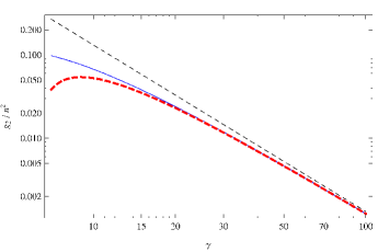
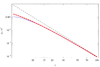
(a)	(b)

Figure 1: Double-logarithmic plots of the $2$-body and $3$-body local correlation functions at zero temperature. These correlation functions measure the probabilities of finding two and three particles at the same place, respectively. (a) A good agreement between our result (55) (thin blue solid line) and the exact Bethe Ansatz result (57) (thick red dashed line) is observed. The thin black dashed line is the leading order of $g_{2}$ given in dmg_gvs . (b) An excellent agreement between our result (55) (thin blue solid line) and the approximate result (60) (thick red dashed line) is observed. The thin black dashed line is the leading order of $g_{3}$ given in dmg_gvs .

IV IV $M$-body wave function at zero collision energy

In this section, we consider the wave function of the 1D interacting bosons at zero collision energy and zero total momentum. If one boson has zero total momentum, its wave function is proportional to

$$\phi^{(1)}(x_{1})\equiv 1.$$ (61)

When two bosons collide with zero total momentum and zero energy, their wave function is proportional to

$$\phi^{(2)}(x_{1},x_{2})\equiv|x_{1}-x_{2}|+A,$$ (62)

where

$$A=\frac{2}{c}.$$ (63)

$(-A)$ is the so-called 1D scattering length.

If $M$ bosons collide with zero total momentum and zero energy, and if we restrict our attention to the case in which their wave function grows no faster than $\rho^{M(M-1)/2}$ at large $\rho$, where $\rho$ is the overall size of the system of $M$ bosons, then their wave function is uniquely determined up to a multiplicative constant. This wave function is proportional to $\phi^{(M)}(x_{1},x_{2},\cdots,x_{M})$. When $x_{1}\leq x_{2}\leq\cdots\leq x_{M}$, for our convenience we define

$$\phi^{(M)}(x_{1},x_{2},\cdots,x_{M}) \equiv\lim_{k\to 0}\frac{1!\,2!\,\cdots(M-1)!}{\prod_{i<j}(\mathrm{i}k_{j}-\mathrm{i}k_{i})}\sum_{p}(-1)^{p}\bigg{[}\prod_{i<j}\Big{(}1-A\frac{\mathrm{i}(k_{pi}-k_{pj})}{2}\Big{)}\bigg{]}$$

$$\quad\times\exp(\mathrm{i}k_{p1}x_{1}+\cdots+\mathrm{i}k_{pM}x_{M}),$$ (64)

where the limit is understood as follows: hold the ratio $k_{1}:\cdots:k_{M}$ constant, and let $k_{1}$, …, $k_{M}$ shrink to zero simultaneously. $p$ is one of the $M!$ permutations, and $(-1)^{p}$ is the signature of the permutation. $(-1)^{p}=+1$ for even permutations and $(-1)^{p}=-1$ for odd permutations. In addition, we define $\phi^{(M)}(x_{1},x_{2},\cdots,x_{M})$ to be completely symmetric under the exchanges of its arguments.

The few-body asymptotic Bethe Ansatz wave functions defined here will help us to understand important correlation effects of the many-body systems.

We have the following explicit formulas at $x_{1}\leq x_{2}\leq\cdots$:

$$\phi^{(1)}(x_{1}) = 1,$$ (65)

$$\phi^{(2)}(x_{1},x_{2}) = (x_{2}-x_{1})+A,$$ (66)

$$\phi^{(3)}(x_{1},x_{2},x_{3}) = (x_{2}-x_{1})(x_{3}-x_{1})(x_{3}-x_{2})$$ (67)

$$+A\big{[}(x_{2}-x_{1})^{2}+4(x_{2}-x_{1})(x_{3}-x_{2})+(x_{3}-x_{2})^{2}\big{]}+3A^{2}(x_{3}-x_{1})+\frac{3}{2}A^{3},$$

$$\phi^{(4)}(x_{1},x_{2},x_{3},x_{4}) = (x_{2}-x_{1})(x_{3}-x_{1})(x_{3}-x_{2})(x_{4}-x_{1})(x_{4}-x_{2})(x_{4}-x_{3})$$ (68)

$$+A\left(\delta_{2}\delta_{3}^{4}+\delta_{4}\delta_{3}^{4}+2\delta_{2}^{2}\delta_{3}^{3}+2\delta_{4}^{2}\delta_{3}^{3}+12\delta_{2}\delta_{4}\delta_{3}^{3}+\delta_{2}^{3}\delta_{3}^{2}+\delta_{4}^{3}\delta_{3}^{2}+15\delta_{2}\delta_{4}^{2}\delta_{3}^{2}\right.$$

$$\left.+15\delta_{2}^{2}\delta_{4}\delta_{3}^{2}+4\delta_{2}\delta_{4}^{3}\delta_{3}+12\delta_{2}^{2}\delta_{4}^{2}\delta_{3}+4\delta_{2}^{3}\delta_{4}\delta_{3}+\delta_{2}^{2}\delta_{4}^{3}+\delta_{2}^{3}\delta_{4}^{2}\right)$$

$$+A^{2}\left(\delta_{3}^{4}+10\delta_{2}\delta_{3}^{3}+10\delta_{4}\delta_{3}^{3}+12\delta_{2}^{2}\delta_{3}^{2}+12\delta_{4}^{2}\delta_{3}^{2}+48\delta_{2}\delta_{4}\delta_{3}^{2}+3\delta_{2}^{3}\delta_{3}\right.$$

$$\left.+3\delta_{4}^{3}\delta_{3}+33\delta_{2}\delta_{4}^{2}\delta_{3}+33\delta_{2}^{2}\delta_{4}\delta_{3}+3\delta_{2}\delta_{4}^{3}+9\delta_{2}^{2}\delta_{4}^{2}+3\delta_{2}^{3}\delta_{4}\right)$$

$$+\frac{1}{2}A^{3}\left(3\delta_{2}^{3}+42\delta_{3}\delta_{2}^{2}+39\delta_{4}\delta_{2}^{2}+66\delta_{3}^{2}\delta_{2}+39\delta_{4}^{2}\delta_{2}+144\delta_{3}\delta_{4}\delta_{2}+16\delta_{3}^{3}\right.$$

$$\left.+3\delta_{4}^{3}+42\delta_{3}\delta_{4}^{2}+66\delta_{3}^{2}\delta_{4}\right)$$

$$+3A^{4}\left(3\delta_{2}^{2}+13\delta_{3}\delta_{2}+11\delta_{4}\delta_{2}+7\delta_{3}^{2}+3\delta_{4}^{2}+13\delta_{3}\delta_{4}\right)$$

$$+\frac{9}{2}A^{5}\left(3\delta_{2}+4\delta_{3}+3\delta_{4}\right)+\frac{9}{2}A^{6},$$

etc, where $\delta_{j}\equiv x_{j}-x_{j-1}$. In general, $\phi^{(M)}(x_{1},\cdots,x_{M})$ is a homogeneous polynomial of $x_{1}$, …, $x_{M}$ and $A$ of degree $M(M-1)/2$ at $x_{1}\leq x_{2}\leq\cdots\leq x_{M}$. One can show that

$$\phi^{(M)}(x_{1},\cdots,x_{M}) =\Big{|}\prod_{i<j}(x_{j}-x_{i})\Big{|}$$

$$\quad+O(A^{1}x^{M(M-1)/2-1})+O(A^{2}x^{M(M-1)/2-2})+\cdots+O(A^{M(M-1)/2-1}x^{1})$$

$$\quad+1!\,2!\,\cdots(M-1)!\,M!\,(A/2)^{M(M-1)/2}.$$ (69)

In particular, we observe

$$\phi^{(M)}(x,\cdots,x)=1!\,2!\,\cdots(M-1)!\,M!\,(A/2)^{M(M-1)/2}.$$ (70)

V V. $M$-body short-distance correlation of the ideal Fermi gas

Consider a spin-polarized 1D ideal Fermi gas with number density $n$ and temperature $T$. It has momentum distribution

$$f(k)=\frac{1}{1+\exp\big{(}\frac{\hbar^{2}k^{2}/2m-\mu}{k_{B}T}\big{)}},$$ (71)

where $m$ is the mass of each fermion, $k_{B}$ is Boltzmann’s constant, $\mu$ is the chemical potential and as before $n=\int_{-\infty}^{\infty}\frac{dk}{2\pi}f(k)$. Using Wick’s theorem, we find that

$$\langle\Psi^{\dagger}(x_{1})\cdots\Psi^{\dagger}(x_{M})\Psi(y_{M})\cdots\Psi(y_{1})\rangle =\sum_{P}(-1)^{P}\int_{-\infty}^{\infty}\frac{dk_{1}}{2\pi}\cdots\frac{dk_{M}}{2\pi}f(k_{1})\cdots f(k_{M})$$

$$\quad\times e^{-(\mathrm{i}k_{1}x_{1}+\cdots+\mathrm{i}k_{M}x_{M})+(\mathrm{i}k_{1}y_{P1}+\cdots+\mathrm{i}k_{M}y_{PM})},$$ (72)

where $\Psi^{\dagger}(x)$ and $\Psi(x)$ are respectively the fermion creation and annihilation operators. When the separations between these $2M$ coordinates are much smaller than both the average inter-particle spacing and the thermal de Broglie wave length, we find

$$\langle\Psi^{\dagger}(x_{1})\cdots\Psi^{\dagger}(x_{M})\Psi(y_{M})\cdots\Psi(y_{1})\rangle =\frac{I_{M}}{[1!\,2!\cdots(M-1)!]^{2}M!}\prod_{i<j}(x_{j}-x_{i})(y_{j}-y_{i})$$

$$\quad+\text{(higher-order terms in the separations)},$$ (73)

where

$$I_{M}\equiv\int\frac{dk_{1}}{2\pi}\cdots\frac{dk_{M}}{2\pi}f(k_{1})\cdots f(k_{M})\Big{[}\prod_{i<j}(k_{j}-k_{i})\Big{]}^{2}.$$ (74)

At zero temperature we may use Eq. (34) and the related formulas in Sec. III to deduce

$$I_{M}=\frac{\big{(}\prod_{j=1}^{M-1}j!\big{)}^{2}\,M!}{\big{[}\prod_{j=1}^{M-1}(2j-1)!!\big{]}^{2}\,(2M-1)!!}\pi^{M(M-1)}n^{M^{2}}.$$ (75)

Let $\hat{n}(x)=\Psi^{\dagger}(x)\Psi(x)$ be the local number density operator. We find that

$$\langle\hat{n}(x_{1})\cdots\hat{n}(x_{M})\rangle=\frac{I_{M}}{[1!\,2!\cdots(M-1)!]^{2}M!}\prod_{i<j}(x_{j}-x_{i})^{2}$$ (76)

plus higher-order terms in the separations, at small but nonzero separations.

VI VI. $M$-body short-distance non-local correlation of the strongly repulsive Bose gas

In this section we concentrate on the non-local $M$-body correlation function of the 1D strongly repulsive Bose gas, with $\gamma=\frac{c}{n}=\frac{2}{nA}\gg 1$ and in the temperature regime $T\ll\gamma^{2}T_{d}$, where $T_{d}\equiv\hbar^{2}n^{2}/(2mk_{B})$ is the quantum degeneracy temperature, and $n$ is the number density. In such a regime, when $x_{1},\cdots,x_{M}$ are sufficiently close to each other, such that their maximum separation is comparable to or less than $A$, but the remaining $(N-M)$ particles are not that close to them, the $N$-body wave function is approximately factorized as

$$\psi(x_{1},\cdots,x_{M},x_{M+1},\cdots,x_{N})\approx\phi^{(M)}(x_{1},\cdots,x_{M})\Phi(\bar{x},x_{M+1},\cdots,x_{N})$$ (77)

plus higher-order corrections, where $\bar{x}=(x_{1}+\cdots+x_{M})/M$.

Assuming that

$$\int dx_{1}\cdots dx_{N}|\psi(x_{1},\cdots,x_{N})|^{2}=1,$$ (78)

we have

$$\langle\Psi^{\dagger}(x_{1})\cdots\Psi^{\dagger}(x_{M})\Psi(y_{M})\cdots\Psi(y_{1})\rangle =\frac{N!}{(N-M)!}\int dx_{M+1}\cdots dx_{N}$$

$$\quad\quad\times\psi^{*}(x_{1},\cdots,x_{M},x_{M+1},\cdots,x_{N})$$

$$\quad\quad\times\psi(y_{1},\cdots,y_{M},x_{M+1},\cdots,x_{N}),$$ (79)

where $\Psi^{\dagger}(x)$ and $\Psi(x)$ are respectively the boson creation and annihilation operators. When the maximum separation of $x_{1},\cdots,x_{M},y_{1},\cdots,y_{M}$ is comparable to or less than $A$, we may substitute Eq. (77) into Eq. (VI) to obtain

$$\langle\Psi^{\dagger}(x_{1})\cdots\Psi^{\dagger}(x_{M})\psi(y_{M})\cdots\Psi(y_{1})\rangle\approx B_{M}\phi^{(M)*}(x_{1},\cdots,x_{M})\phi^{(M)}(y_{1},\cdots,y_{M}),$$ (80)

where

$$B_{M}=\frac{N!}{(N-M)!}\int dx_{M+1}\cdots dx_{N}\big{|}\Phi(\bar{x},x_{M+1},\cdots,x_{N})\big{|}^{2}.$$ (81)

We have ignored the tiny difference between $\bar{x}$ and $\bar{y}$ in Eq. (80). If the total momentum of the system is zero, $B_{M}$ is independent of $\bar{x}$.

A special case of Eq. (80) is

$$\langle\hat{n}(x_{1})\cdots\hat{n}(x_{M})\rangle\approx B_{M}\big{|}\phi^{(M)}(x_{1},\cdots,x_{M})\big{|}^{2},$$ (82)

if the coordinates $x_{1},\cdots,x_{M}$ do not coincide. Here $\hat{n}(x)$ is the local number density operator of the bosons.

When the separations between $x_{1},\cdots,x_{M}$ are much larger than $A$, but much smaller than both the average inter-particle spacing and the thermal de Broglie wave length, we can use our knowledge of $\phi^{(M)}$ to deduce that

$$\langle\hat{n}(x_{1})\cdots\hat{n}(x_{M})\rangle\approx B_{M}\prod_{i<j}(x_{j}-x_{i})^{2}.$$

Comparing the above formula with our result for the ideal Fermi gas [see Eq. (76)], we get

$$B_{M}=\frac{I_{M}}{[1!\,2!\cdots(M-1)!]^{2}M!}.$$ (83)

Therefore, when the separations between $x_{1},\cdots,x_{M},y_{1},\cdots,y_{M}$ are much smaller than both the average inter-particle spacing and the thermal de Broglie wave length, we get

$$\langle\Psi^{\dagger}(x_{1})\cdots\Psi^{\dagger}(x_{M})\Psi(y_{M})\cdots\Psi(y_{1})\rangle\approx\frac{I_{M}}{[1!\,2!\cdots(M-1)!]^{2}M!}\phi^{(M)*}(x_{1},\cdots,x_{M})\phi^{(M)}(y_{1},\cdots,y_{M}),$$ (84)

where $\phi^{(M)}$ is defined in Sec. IV. At zero temperature, $I_{M}$ is given by Eq. (75). At nonzero temperatures $T\ll\gamma^{2}T_{d}$, one can use Eq. (74) to calculate $I_{M}$. When $T\gtrsim\gamma^{2}T_{d}$, Eq. (84) breaks down. We emphasize that Eq. (84) is a key result of this paper.

When the above $2M$ coordinates are all equal, we get

$$\langle\big{[}\Psi^{\dagger}(x)\big{]}^{M}\big{[}\Psi(x)\big{]}^{M}\rangle\approx M!\,I_{M}(A/2)^{M(M-1)}.$$ (85)

At zero temperature, using Eq. (75) we find

$$\frac{\langle\big{[}\Psi^{\dagger}(x)\big{]}^{M}\big{[}\Psi(x)\big{]}^{M}\rangle}{n^{M}}=\frac{\big{[}\prod_{j=1}^{M}(j!)\big{]}^{2}}{\big{[}\prod_{j=1}^{M-1}(2j-1)!!\big{]}^{2}(2M-1)!!}\Big{(}\frac{\pi}{\gamma}\Big{)}^{M(M-1)}+o(\gamma^{-M(M-1)})~{}~{}~{}\text{at }T=0,$$ (86)

which is consistent with Eq. (48).

VII VII. Conclusions

Higher-order quantum correlations reveal the quantum many-body effects in ultracold atomic gases yanli . In light of Gangardt and Shlyapnikov’s method for calculating the higher-order correlation functions of 1D bosons with an infinitely strong interaction, we have rigorously calculated the $M$-body correlation function. It turns out that the quasimomentum distribution correction $\alpha=1-2/\gamma$ to the free fermions leads to the sub-leading terms in the $M$-body correlation functions at a large interaction strength. We have calculated the higher-order local correlation functions in terms of the statistical parameter $\alpha$ and obtained $g_{M}$ explicitly for arbitrary $M$ with sub-leading order terms. These results not only recover the expressions for $g_{2}$ and $g_{3}$ with the sub-leading terms given in the literature dmg_gvs ; dmg_gvs1 ; Kheruntsyan ; Cazalilla ; Kormos:2009 but also provide explicit forms of $g_{M}$ with arbitrary $M$ at zero and nonzero temperatures. To our best knowledge, there is not yet another such analytical expression of the local correlation functions $g_{M}$ (51) for $M>3$ in the literature for the 1D Bose gas footnote2 . Moreover, we have explicitly calculated the short-distance non-local $M$-body correlation functions of the 1D free fermions and the 1D strongly interacting bosons in Eqs. (73) and (84). Our results provide new insights into the many-body correlations in quantum systems of interacting bosons and noninteracting fermions.

VIII APPENDIX I

In the strong coupling limit, $\gamma\gg 1$, the higher-order correlation function is given by Eq. (4),

$$g_{M}=\frac{N!}{(N-M)!}\frac{\int|\psi(0,\cdots,0,x_{M+1},\cdots,x_{N})|^{2}dx_{M+1}\cdots dx_{N}}{\int|\psi(x_{1},\cdots,x_{N})|^{2}dx_{1}\cdots dx_{N}}.$$

VIII.1 Calculating the numerator of the formula

The Bethe Ansatz energy eigenfunction in the domain $0\leq x_{1}\leq x_{2}\leq\cdots\leq x_{N}\leq L$ is

$$\psi(x_{1},x_{2},\cdots,x_{N}) =\sum\limits_{p}(-1)^{p}\Big{[}\prod\limits_{1\leq i<j\leq N}\Big{(}1+\frac{\mathrm{i}k_{p{j}}-\mathrm{i}k_{p{i}}}{c}\Big{)}\Big{]}\exp\Big{(}\sum\limits_{j=1}^{N}\mathrm{i}k_{p{j}}x_{j}\Big{)}$$

$$=\Big{[}\prod\limits_{1\leq i<j\leq N}\Big{(}1+\frac{\partial_{x_{j}}-\partial_{x_{i}}}{c}\Big{)}\Big{]}\phi^{(0)}(x_{1},\cdots,x_{N})$$ (87)

where

$$\phi^{(0)}(x_{1},\cdots,x_{N})\equiv\sum\limits_{p}(-1)^{p}\exp\Big{(}\sum\limits_{j=1}^{N}\mathrm{i}k_{pj}x_{j}\Big{)},\quad\text{for all }x$$ (88)

is completely antisymmetric under the exchange of its arguments. The function

$$\prod\limits_{1\leq i\leq M;M+1\leq j\leq N}\Big{(}1+\frac{\partial_{x_{j}}-\partial_{x_{i}}}{c}\Big{)}\prod\limits_{M+1\leq i<j\leq N}\Big{(}1+\frac{\partial_{x_{j}}-\partial_{x_{i}}}{c}\Big{)}\phi^{(0)}(x_{1},\cdots,x_{N})$$ (89)

is still antisymmetric under the exchange of any two coordinates $x_{i}$ and $x_{j}$ satisfying $1\leq i<j\leq M.$ Being smooth, such a function must vanish like $\delta^{M(M-1)/2}$ (or even faster) when the coordinates $x_{1},\cdots,x_{M}$ are of the order $\delta$ and $\delta$ goes to zero. Therefore, in the domain $0\leq x_{M+1}\leq x_{M+2}\leq\cdots\leq x_{N}\leq L$ we have

$$\psi(0,\cdots,0,x_{M+1},\cdots,x_{N}) =\prod_{1\leq i<j\leq M}\frac{\partial_{x_{j}}-\partial_{x_{i}}}{c}\prod_{1\leq i\leq M;M+1\leq j\leq N}\Big{(}1+\frac{\partial_{x_{j}}-\partial_{x_{i}}}{c}\Big{)}$$

$$\mspace{10.0mu}\prod_{M+1\leq i<j\leq N}\Big{(}1+\frac{\partial_{x_{j}}-\partial_{x_{i}}}{c}\Big{)}\phi^{(0)}(x_{1},\cdots,x_{N})\Big{|}_{x_{1}=\cdots=x_{M}=0}.$$ (90)

At strong coupling, $c\to\infty$, we expand Eq. (VIII.1) as

$$\psi(0,\cdots,0,x_{M+1},\cdots,x_{N})=\chi^{(0)}(x_{M+1},\cdots,x_{N})+\chi^{(1)}(x_{M+1},\cdots,x_{N})+O(c^{-M(M-1)/2-2}).$$ (91)

In the domain $0\leq x_{M+1}\leq x_{M+2}\leq\cdots\leq x_{N}\leq L$ we have

$$\chi^{(0)}(x_{M+1},\cdots,x_{N}) =c^{-M(M-1)/2}\Big{[}\prod\limits_{1\leq i<j\leq M}\Big{(}\partial_{x_{j}}-\partial_{x_{i}}\Big{)}\Big{]}\phi^{(0)}(x_{1},\cdots,x_{N})\Big{|}_{x_{1}=\cdots=x_{M}=0},$$ (92)

$$\text{and}\quad\chi^{(1)}(x_{M+1},\cdots,x_{N}) =c^{-M(M-1)/2-1}\Big{[}-(N-M)\sum\limits_{l=1}^{M}\partial_{x_{l}}+\sum\limits_{l=M+1}^{N}(2l-N-1)\partial_{x_{l}}\Big{]}$$

$$\quad\Big{[}\prod\limits_{1\leq i<j\leq M}\Big{(}\partial_{x_{j}}-\partial_{x_{i}}\Big{)}\Big{]}\phi^{(0)}(x_{1},\cdots,x_{N})\Big{|}_{x_{1}=\cdots=x_{M}=0}.$$ (93)

Let

$$\phi^{(\Delta)}(\epsilon,x_{M+1},\cdots,x_{N})\equiv\Big{[}\prod_{1\leq i<j\leq M}(\partial_{x_{j}}-\partial_{x_{i}})\Big{]}\phi^{(0)}(x_{1},\cdots,x_{N})\Big{|}_{x_{1}=\cdots=x_{M}=\epsilon}.$$ (94)

Then in the domain $0\leq x_{M+1}\leq x_{M+2}\leq\cdots\leq x_{N}\leq L$ Eq. (92) and Eq. (93) become

$$\chi^{(0)}(x_{M+1},\cdots,x_{N}) =c^{-M(M-1)/2}\phi^{(\Delta)}(0,x_{M+1},\cdots,x_{N}),$$ (95)

$$\text{and}\quad\chi^{(1)}(x_{M+1},\cdots,x_{N}) =c^{-M(M-1)/2-1}\Big{[}-(N-M)\frac{\partial\phi^{(\Delta)}(\epsilon,x_{M+1},\cdots,x_{N})}{\partial\epsilon}\Big{|}_{\epsilon=0}$$

$$\quad+\sum\limits_{l=M+1}^{N}(2l-N-1)\frac{\partial\phi^{(\Delta)}(0,x_{M+1},\cdots,x_{N})}{\partial x_{l}}\Big{]}.$$ (96)

Therefore, in the domain $0\leq x_{M+1}\leq x_{M+2}\leq\cdots\leq x_{N}\leq L$ we have

$$|\psi(0,\cdots,0,x_{M+1},\cdots,x_{N})|^{2} =|\chi^{(0)}|^{2}+\chi^{(0)*}\chi^{(1)}+\chi^{(0)}\chi^{(1)*}+O(c^{-M(M-1)-2})$$

$$=c^{-M(M-1)}|\phi^{(\Delta)}(0,x_{M+1},\cdots,x_{N})|^{2}$$

$$\quad+c^{-M(M-1)-1}\Big{[}-(N-M)\frac{\partial|\phi^{(\Delta)}(\epsilon,x_{M+1},\cdots,x_{N})|^{2}}{\partial\epsilon}\Big{|}_{\epsilon=0}$$

$$\quad+\sum\limits_{l=M+1}^{N}(2l-N-1)\frac{\partial|\phi^{(\Delta)}(0,x_{M+1},\cdots,x_{N})|^{2}}{\partial x_{l}}\Big{]}+O(c^{-M(M-1)-2}).$$ (97)

Let

$$\rho^{(\Delta)}(\epsilon) \equiv\int_{0\leq x_{M+1}\leq\cdots\leq x_{N}\leq L}|\phi^{(\Delta)}(\epsilon,x_{M+1},\cdots,x_{N})|^{2}dx_{M+1}\cdots dx_{N},$$ (98)

$$\rho^{(\Delta)}_{l}(x_{l}) \equiv\int_{0\leq x_{M+1}\leq\cdots\leq x_{N}\leq L}|\phi^{(\Delta)}(0,x_{M+1},\cdots,x_{N})|^{2}dx_{M+1}\cdots dx_{l-1}dx_{l+1}\cdots dx_{N},$$ (99)

where $M+1\leq l\leq N.$ Then

$$\int_{0\leq x_{M+1}\leq\cdots\leq x_{N}\leq L}|\psi(0,\cdots,0,x_{M+1},\cdots,x_{N})|^{2}dx_{M+1}\cdots dx_{N}$$

$$=c^{-M(M-1)}\rho^{(\Delta)}(0)+c^{-M(M-1)-1}\bigg{\{}-(N-M)\frac{\partial\rho^{(\Delta)}(\epsilon)}{\partial\epsilon}\Big{|}_{\epsilon=0}+\sum\limits_{l=M+1}^{N}(2l-N-1)\Big{[}\rho^{(\Delta)}_{l}(L)-\rho^{(\Delta)}_{l}(0)\Big{]}\bigg{\}}$$

$$\quad\quad+O(c^{-M(M-1)-2}).$$ (100)

At leading order in $1/c$, the quasimomenta $k_{j}\;(1\leq j\leq N)$ may be approximated as $(2\pi/L)\times$integers. This implies that $\rho^{(\Delta)}(\epsilon)$ is independent of $\epsilon$ at leading order in $1/c,$ and

$$\frac{\partial\rho^{(\Delta)}(\epsilon)}{\partial\epsilon}\Big{|}_{\epsilon=0}=O(1/c).$$ (101)

Consideration of the volumes of the domain of integration indicate that

$$\rho^{(\Delta)}_{l}(0)=0, \quad\text{if}\;M+2\leq l\leq N,$$ (102)

$$\rho^{(\Delta)}_{l}(L)=0, \quad\text{if}\;M+1\leq l\leq N-1.$$ (103)

Because of the smoothness and the complete antisymmetry of $\phi^{(0)}(x_{1},\cdots,x_{N}),$ it is easy to see that when $x_{M+1}\rightarrow 0,$ the function $\phi^{(\Delta)}(0,x_{M+1},\cdots,x_{N})$ vanishes like $x^{M}_{M+1}\rightarrow 0.$ Consequently

$$\rho^{(\Delta)}_{M+1}(0)=0.$$ (104)

Finally,

$$\rho^{(\Delta)}_{N}(L) =\int_{0\leq x_{M+1}\leq\cdots\leq x_{N-1}\leq L}|\phi^{(\Delta)}(0,x_{M+1},\cdots,x_{N-1},L)|^{2}dx_{M+1}\cdots dx_{N-1}$$

$$=\int_{0\leq x_{M+1}\leq\cdots\leq x_{N-1}\leq L}|\phi^{(\Delta)}(0,x_{M+1},\cdots,x_{N-1},0)+O(1/c)|^{2}dx_{M+1}\cdots dx_{N-1}$$

$$=\int_{0\leq x_{M+1}\leq\cdots\leq x_{N-1}\leq L}|O(1/c)|^{2}dx_{M+1}\cdots dx_{N-1}$$

$$=O(1/c^{2}).$$ (105)

Combining the above findings, we simplify Eq. (VIII.1) as

$$\int_{0\leq x_{M+1}\leq\cdots\leq x_{N}\leq L}|\psi(0,\cdots,0,x_{M+1},\cdots,x_{N})|^{2}dx_{M+1}\cdots dx_{N}$$

$$=c^{-M(M-1)}\rho^{(\Delta)}(0)+O(c^{-M(M-1)-2})$$

$$=c^{-M(M-1)}\int_{0\leq x_{M+1}\leq\cdots\leq x_{N}\leq L}|\phi^{(\Delta)}(0,x_{M+1},\cdots,x_{N})|^{2}dx_{M+1}\cdots dx_{N}+O(c^{-M(M-1)-2}).$$ (106)

Multiplying the above equation by $(N-M)!$, we get

$$\int_{0}^{L}|\psi(0,\cdots,0,x_{M+1},\cdots,x_{N})|^{2}dx_{M+1}\cdots dx_{N}$$

$$=c^{-M(M-1)}\int_{0}^{L}|\phi^{(\Delta)}(0,x_{M+1},\cdots,x_{N})|^{2}dx_{M+1}\cdots dx_{N}+O(c^{-M(M-1)-2}).$$ (107)

VIII.2 Calculating the denominator of the formula

At strong coupling, $c\to\infty$, we expand Eq. (VIII.1) as

$$\psi(x_{1},\cdots,x_{N})=\psi^{(0)}(x_{1},\cdots,x_{N})+\psi^{(1)}(x_{1},\cdots,x_{N})+O(c^{-2}),$$ (108)

where in the domain $0\leq x_{1}\leq x_{2}\leq\cdots\leq x_{N}\leq L$ we have

$$\psi^{(0)}(x_{1},\cdots,x_{N}) =\sum_{p}(-1)^{p}\exp\Big{(}\sum_{j=1}^{N}\mathrm{i}k_{p{j}}x_{j}\Big{)},$$ (109)

$$\text{and}\quad\psi^{(1)}(x_{1},\cdots,x_{N}) =\sum_{1\leq i<j\leq N}\frac{(\partial_{x_{j}}-\partial_{x_{i}})}{c}\psi^{(0)}(x_{1},\cdots,x_{N})$$

$$=\frac{1}{c}\sum_{j=1}^{N}(2j-N-1)\partial_{x_{j}}\psi^{(0)}(x_{1},\cdots,x_{N}).$$ (110)

Therefore

$$\int_{0}^{L}|\psi(x_{1},\cdots,x_{N})|^{2}dx_{1}\cdots dx_{N} =N!\int_{0\leq x_{1}\leq\cdots\leq x_{N}\leq L}\big{|}\psi^{(0)}+\psi^{(1)}\big{|}^{2}dx_{1}\cdots dx_{N}+O(c^{-2})$$

$$=N!\int_{0\leq x_{1}\leq\cdots\leq x_{N}\leq L}\Big{[}|\psi^{(0)}|^{2}+\Big{(}\psi^{(0)*}\psi^{(1)}+\psi^{(0)}\psi^{(1)*}\Big{)}\Big{]}dx_{1}\cdots dx_{N}+O(c^{-2})$$

$$=N!\int_{0\leq x_{1}\leq\cdots\leq x_{N}\leq L}|\psi^{(0)}|^{2}dx_{1}\cdots dx_{N}+\frac{2(N!)}{c}\sum_{j=1}^{N}(2j-N-1)\operatorname{Re}b_{j}+O(c^{-2}),$$ (111)

where

$$b_{j}\equiv\int_{0\leq x_{1}\leq\cdots\leq x_{N}\leq L}\psi^{(0)*}\partial_{x_{j}}\psi^{(0)}dx_{1}\cdots dx_{N}.$$ (112)

Since the total momentum $(k_{1}+\cdots+k_{N})$ must be an integer times $(2\pi/L)$, it is easy to see that when $0\leq x_{1}\leq\cdots\leq x_{N}\leq L$, we have

$$\psi^{(0)}(L-x_{N},L-x_{N-1},\cdots,L-x_{1}) =\sum_{p}(-1)^{p}\exp\Big{[}\mathrm{i}\sum_{j=1}^{N}k_{p{j}}(L-x_{N-j+1})\Big{]}$$

$$=\sum_{p}(-1)^{p}\exp\big{(}-\mathrm{i}\sum_{j=1}^{N}k_{p{j}}x_{N-j+1}\big{)}$$

$$=(-1)^{r}\psi^{(0)*}(x_{1},x_{2},\cdots,x_{N}),$$ (113)

where $(-1)^{r}$ is the signature of the reversal permutation $\{1,\cdots,N\}\to\{N,\cdots,1\}$. In particular, $(-1)^{r}=+1$ if $\mathrm{mod}(N,4)=0$ or 1, and $(-1)^{r}=-1$ if $\mathrm{mod}(N,4)=2$ or 3.

From the above equation one can show that

$$b_{N+1-j}=-b_{j}^{*}.$$ (114)

Define

$$\rho_{j}(x)=\int_{0\leq x_{1}\leq\cdots\leq x_{j-1}\leq x\leq x_{j+1}\leq\cdots\leq x_{N}\leq L}|\psi^{(0)}(x_{1},\cdots,x_{j-1},x,x_{j+1},\cdots,x_{N})|^{2}dx_{1}\cdots dx_{j-1}dx_{j+1}\cdots dx_{N}.$$ (115)

It is easy to see that

$$2\operatorname{Re}b_{j}=\int_{0}^{L}\frac{\partial\rho_{j}(x)}{\partial x}dx=\rho_{j}(L)-\rho_{j}(0).$$ (116)

From the definition of $\rho_{j}(x)$ we can easily see that

$$\rho_{j}(0) =0,\quad\text{if}\;j\geq 2,$$ (117)

$$\text{and}\quad\rho_{j}(L) =0,\quad\text{if}\;j\leq N-1.$$ (118)

It is also easy to see that

$$\rho_{1}(0)=\rho_{N}(L).$$ (119)

Thus

$$2\operatorname{Re}b_{j}=0,~{}~{}\text{if }2\leq j\leq N-1,$$ (120)

and, assuming that $N\geq 2$, we have

$$2\operatorname{Re}b_{1} =-\rho_{N}(L),$$ (121)

$$2\operatorname{Re}b_{N} =+\rho_{N}(L).$$ (122)

So, Eq. (VIII.2) is simplified as

$$\int_{0}^{L}|\psi(x_{1},\cdots,x_{N})|^{2}dx_{1}\cdots dx_{N}=\int_{0}^{L}|\psi^{(0)}|^{2}dx_{1}\cdots dx_{N}+\frac{N!\,2(N-1)}{c}\rho_{N}(L)+O(c^{-2}).$$ (123)

Let

$$\rho_{\text{arb}}(x)\equiv\int_{0}^{L}|\psi^{(0)}(x_{1},\cdots,x_{N-1},x)|^{2}dx_{1}\cdots dx_{N-1}.$$ (124)

Strictly speaking, $\rho_{\text{arb}}(x)$ depends on $x$. But in the large $c$ limit if we approximate $\psi^{(0)}$ by $\psi$, then $\rho_{\text{arb}}(x)$ is approximately proportional to the local number density, which is a constant at thermal equilibrium. Thus

$$\rho_{\text{arb}}(x)=\big{[}1+O(1/c)\big{]}\frac{1}{L}\int_{0}^{L}\rho_{\text{arb}}(y)dy=\big{[}1+O(1/c)\big{]}\frac{1}{L}\int_{0}^{L}|\psi^{(0)}|^{2}dx_{1}\cdots dx_{N},~{}~{}\text{if }0\leq x\leq L.$$ (125)

On the other hand, it is easy to see that

$$\rho_{N}(L)=\frac{1}{(N-1)!}\rho_{\text{arb}}(L).$$ (126)

Thus, in the limit $c\to\infty$ we have

$$\int_{0}^{L}|\psi(x_{1},\cdots,x_{N})|^{2}dx_{1}\cdots dx_{N}=\Big{[}1+\frac{2N(N-1)}{cL}+O(c^{-2})\Big{]}\int_{0}^{L}|\psi^{(0)}|^{2}dx_{1}\cdots dx_{N}.$$ (127)

Acknowledgments

The authors thank M. Kormos and M. Rigol for helpful discussions. This work has been supported by the NNSFC under grant numbers 11374331 and by the key NNSFC grant No. 11534014. The author ST is supported by the U.S. National Science Foundation CAREER award Grant No. PHY-1352208. This work also has been partially supported by CAS-TWAS President’s Fellowship for International PhD students. The author RR was funded by Chinese Academy of Science President’s International Fellowship Initiative grant No.2015VMA011.

References

• (1) D. M. Gangardt and G. V. Shlyapnikov 2003 Phys. Rev. Lett. 90 , 010401.
• (2) D.M. Gangardt and G. V. Shlyapnikov 2003 New Journal of Physics, 5, 79.
• (3) Vadim V. Cheianov, H. Smith and M. B. Zvonarev 2006 Phy. Rev.A, 73, 051604(R).
• (4) Kormos M., Mussardo G., and Trombettoni A. 2009 Phys. Rev. Lett. 103 210404.
• (5) M.-S. Wang, J.-W. Huang, C.-H.Lee, X.-G.Yin, X.-W.Guan and M.T. Batchelor 2013 Phys. Rev. A ,87 , 043634.
• (6) M. Girardeau 1960 J. Math. Phys. 1, 516.
• (7) Yukalov V. I. and Girardeau M. D. 2005 Laser Phys. Lett. 2, 375.
• (8) E.H. Lieb and W. Liniger 1963 Phys.Rev.Lett., 130 1605.
• (9) L. Tonks 1936 Phys. Rev. 50, 955.
• (10) M. D. Girardeau, and A. Minguzzi 2007 Phys. Rev. Lett. 99, 230402.
• (11) A. G. Volosniev, D. V. Fedorov, A. S. Jensen, M. Valiente, and N. T. Zinner 2014 Nature Communications 5, 5300.
• (12) F. Deuretzbacher, D. Becker, J. Bjerlin, S. M. Reimann, and L. Santos 2014 Phys. Rev. A 90, 013611.
• (13) L. Yang, L. Guan, and H. Pu 2015 Phys. Rev. A 91, 043634.
• (14) J. Levinsen, P. Massignan, G. M. Bruun, M. M. Parish 2015 Science Advances 1 , e1500197.
• (15) A. G. Volosniev, D. Petrosyan, M. Valiente, D. V. Fedorov, A. S. Jensen, and N. T. Zinner 2015 Phys. Rev. A 91 , 023620.
• (16) P. Massignan, J. Levinsen, and M. M. Parish 2015 Phys. Rev. Lett. 115, 247202 (2015).
• (17) L. Yang and X. Cui, arxiv: 1510.06087.
• (18) F .D. M. Haldane 1991 Phys. Rev. Lett., 67, 937.
• (19) Serguei B. Isakov, Daniel P. Arovas, Jan Myrhein and Alexios P. Polychronakos 1996 Phys. Lett. A 212, 9601.
• (20) Yomg-Shi Wu 1994 Phy.Rev.Lett., 73, 023010;
D. Bernard and Y.-S. Wu, arXiv:cond-mat/9404025.
• (21) C.N. Yang and C.P. Yang 1969 J. Math. Phys, 10, 1115.
• (22) M. T. Batchelor and X.-W. Guan 2007 Laser Phys. Lett. 4, 77.
• (23) M.T. Batchelor, X.W. Guan and N. Oelkers 2006 Phy. Rev. Lett.,96, 210402.
• (24) Anjan Kundu 1999 Phys. Rev. Lett., 83, 1275.
• (25) A.G. Sykes, D.M.Gangardt, M.J.Davis, K.Viering, M.G. Raizen and K.V. Kheruntsyan, 2008 Phy. Rev. Lett., 100 , 160406.
• (26) Yan Li and Nao-Sheng Qiao 2013 J.At. Mol. Sci., 5 2.
• (27) R. G. Dall, A. G. Manning, S. S. Hodgman, Wu RuGway, K. V. Kheruntsyan and A. G. Truscott, 2013 Nature Phys. 9, 341.
• (28) S. S. Hodgman R. G. Dall, A. G. Manning, K. G. H. Baldwin and A. G. Truscott, 2011 Science 331, 1046.
• (29) B. Laburthe Tolra, K.M.O’Hara, J.H.Huckans, W.D.Phillips, S.L.Rolston and J.V.Porto 2004 Phys. Rev.Lett., 92 190401.
• (30) Toshiya Kinoshita, Trevor Wenger and David S. Weiss, Phys.Rev.Lett., 95 190406 (4 Nov. 2005).
• (31) T. Kinoshita, T. Wenger and D. S. Weiss 2004 Science 305, 1125.
• (32) Maxim Olshanii and Vanja Dunjko 2003 New J. Phys., 5, 98.
• (33) V. E. Korepin, A. G. Izergin and N. M. Bogoliubov 1993 Quantum Inverse Scattering Method and Correlation Functions (Cambridge: Cambridge University Press).
• (34) M.Holzmann and Y castin 1999 Eur. Phys. J. D, 7, 425.
• (35) K.V. Kheruntsyan, D.M. Gangardt, P.D. Drummond and G.V. Shlyapnikov, arXiv:cond-mat/0212153v4, (28 Jul 2003).
• (36) K. K. Kozlowski, J. K. Maillet and N. A. Slavnov 2011 J. Stat.Mech.: Theor and Exp., P03018.
• (37) M.Eckart, R. Walser, W.P Schleich, S Zöllner and P Schmelcher 2009 New J. Phys., 11 023010.
• (38) Ovidiu P. patu, Vladimir E. Korepin and Dmitri V. Averin 2007 J.Phys. A: Math.Theor., 40 023010.
• (39) V.E. Korepin, 1984 Commum. Math.Phys., 94, 023010.
• (40) Oleksandr Gamayun, Andrei G. Pronko and MIkhail B. Zvonarev, arXiv:1511.05922v1 , (2015).
• (41) Kormos M., Mussardo G., and Trombettoni A. 2010 Phys. Rev. A 81, 043606.
• (42) Kormos M., Chou Y.-Z., and Imambekov A. 2011 Phys. Rev. Lett. 107, 230405.
• (43) Pozsgay B. 2011 J. Stat. Mech. P11017.
• (44) García-March M. A., Juliá-Díaz B., Astrakharchik G. E., Busch Th., Boronat J. and Polls A. 2014 New J. Phys. 16, 103004.
• (45) Xu L. and Rigol M. 2015 Phys. Rev. A 92, 063623.
• (46) X.-W. Guan and M. T. Batchlor 2011 J. Phys. A 44, 102001.
• (47) E. Haller and M. Rabie, M. J. Mark, J. G. Danzl, R. Hart, K.Lauber, G. Pupillo and H.-C. Nägerl 2011 Phys. Rev. Lett. , 107 230404.
• (48) J. Armijo, T. Jacqmin, K. V. Kheruntsyan and I. Bouchoule 2010 Phys. Rev.Lett., 105 , 230402.
• (49) P. Makotyn, C. E. Klauss, D. L. Goldberger, E. A. Cornell and D. S. Jin, Nat. Phys. 10, 116 (2014).
• (50) M. Kira, Nat. Comms. 6, 6624 (2015).
• (51) K. V. Kheruntsyan, D. M. Gangardt, P. D. Drummond, and G. V. Shlyapnikov 2003 Phys. Rev. Lett. 91, 040403.
• (52) M. A. Cazalilla 2003 Phys. Rev. A 67, 053606.
• (53) Y.-Z. Jiang, Y.-Y. Chen and X.-W. Guan Guan 2015 Chin. Phys. B, 24, 050311.
• (54) M. Gaudin (1971) J. Math.Phys. , 12 , 1674.
• (55) Madan Lal Mehta, Random matrices-3rd (1970). Elsever academy press,
• (56) V. Freilikher, E. Kanzieper and I. Yurkevich, 1996 Phys. Rev. E 54, 210.
• (57) Wung-Hong Huang, arXiv:cond-mat/0702070v1.
• (58) Raoul Santachiara and Pasquale Calabrase, 2008 J. Stat. Mech. P06005.
• (59) T. Usui, 1960 Prog. Theor. Phys. 23, 787.
• (60) The integral form of $M$-body local correlation functions, Eq. (28) with $\alpha$ set to $1$, was presented in Refs. dmg_gvs ; Pozsgay:2011 .