Quasiperiodic driving of Anderson localized waves in one dimension

Abstract

We consider a quantum particle in a one-dimensional disordered lattice with Anderson localization, in the presence of multi-frequency perturbations of the onsite energies. Using the Floquet representation, we transform the eigenvalue problem into a Wannier-Stark basis. Each frequency component contributes either to a single channel or a multi-channel connectivity along the lattice, depending on the control parameters. The single channel regime is essentially equivalent to the undriven case. The multi-channel driving substantially increases the localization length for slow driving, showing two different scaling regimes of weak and strong driving, yet the localization length stays finite for a finite number of frequency components.

I Introduction

Disordered systems have been of large interest for transport phenomena since Anderson predicted that waves localize in the presence of uncorrelated random potentials Anderson58 . By obtaining the exponential decay of every eigenstate of a disordered class of one dimensional linear wave equations, Anderson proved the localization of a single quantum particle, within a finite volume of the chain, due to disorder. Ever since then, theoretical studies have been performed on higher dimensional lattices in random potentials, showing absence of diffusion in the two dimensional case Abrahams79 , and mobility edges between the insulating and the metallic phase in the three dimensional case Bulka85 . In one dimension, Anderson localization has been observed in experiments with light waves Lahini08 and atomic Bose-Einstein condensates Billy08 ; Roati08 , enhancing further interest in theoretical research of disordered systems.

Wave localization inherently relies on the phase coherence within the wave state. If the disordered potential is allowed to temporarily fluctuate in a random way, phase coherence is lost, and the previously localized wave starts to diffuse without limits Rayanov13 . Assuming that the temporal fluctuations are represented as a quasiperiodic function of time with $D$ incommensurate fundamental frequencies, the random noise can be effectively reached in the limit of $D\rightarrow\infty$. Here we address the case of a finite number of frequencies (colors) $D$. Will the localization length $\zeta$ stay finite for any finite $D$? If yes, what is its dependence on $D$? At fixed $D$ how does $\zeta$ depend on the remaining control parameters, such as frequency, fluctuation amplitude and disorder strength?

A series of computational studies was devoted to this very issue Yamada93 ; Yamada98 ; Yamada99 . While the first conclusion was that Anderson localization can be destroyed for $D\geq 2$, a more accurate recomputation showed that the localization length might well increase, yet stay finite. Other studies focused on the case of single color $D=1$ and computed conductance through small finite systems, without clear conclusions on the localization length Martinez06 ; Kitagawa12 .

In this work we first consider a single frequency color, that is a time-periodic drive. We use the Floquet representation to arrive at a time-independent eigenvalue problem on a two-dimensional lattice, with one direction corresponding to the original spatial extension, and the second one to the Floquet (driving) one. We transform into a Wannier-Stark basis which is diagonal along the Floquet direction, and analyze the resulting eigenvalue problem. For large driving frequencies the equations reduce to uncoupled single channel ones, which are essentially equivalent to the undriven case. For small driving frequencies we obtain a multi-channel regime with a substantial increase of the localization length, and its divergence in the limit of vanishing frequency. This multi-channel regime divides into two further regimes of weak and strong driving amplitudes, which yield different scaling laws. We then generalize to the case of many incommensurate frequencies, and compare our findings to numerical results.

The paper is organized as following. In Sec. II we introduce the model and its general features. In Sec. III we derive the results for one frequency (color) drive. We generalize to many colors in Sec. IV, and discuss numerical results in Sec. V. We conclude with discussions, a summary, and an outlook.

II Model

We consider a disordered one-dimensional tight-binding chain in the presence of a coherent time-dependent driving of the onsite energies. The equations of motion read

$$i\dot{\psi_{l}}=\epsilon_{l}\bigg{[}1+\sum_{i=1}^{D}\mu_{i}\cos(\omega_{i}t+\phi_{l}^{i})\bigg{]}\psi_{l}-\lambda(\psi_{l+1}+\psi_{l-1})\ ,$$ (1)

The onsite energies of each lattice site $\epsilon_{l}$ are random uncorrelated numbers with a probability density function (PDF) of value $1/W$ inside the interval $\epsilon_{l}\in[-W/2,+W/2]$ and zero outside. The parameter $W$ parametrizes the strength of the disorder. The coefficient $\lambda$ is the strength of the hopping between nearest neighbor lattice sites, while $\mu_{i}$ and $\omega_{i}$ respectively are the amplitude and frequency of the $i$-th driving. $D$ is the total number of frequencies (colors) in the driving. The frequencies $\Omega=(\omega_{1},\dots,\omega_{D})$ are chosen incommensurate with each other

$${\mathbf{k}\cdot\Omega}=k_{1}\omega_{1}+\dots+k_{D}\omega_{D}\neq 0\ ,\quad\forall\ {\bf k}\in\mathbb{Z}^{D}\setminus\{0\}\ .$$ (2)

The random phases $\phi_{l}$ are uncorrelated and have a PDF of value $1/(2\pi)$ inside the irreducible interval $\phi_{l}\in[-\pi,\pi]$. Their presence ensures broken time reversal symmetry of (1). For $\mu_{i}=0$, Eq. (1) reduces to the well-known Anderson model with all eigenstates being localized with a finite upper bound on the localization length Anderson58 ; Kramer93 .

III One color

We first consider a driving with only one frequency $D=1$. In this case, Eq.(1) reads

$$i\dot{\psi_{l}}=\epsilon_{l}\left(1+\mu\cos(\omega t+\phi_{l})\right)\psi_{l}-\lambda(\psi_{l+1}+\psi_{l-1})~{}.$$ (3)

Since the perturbation is time periodic with period $T=\frac{2\pi}{\omega}$, we first perform a Floquet expansion which will yield an effective two-dimensional lattice problem.

III.1 From Floquet to Wannier-Stark

According to the Floquet theorem Floquet83 ; Shirley65 , a solution of (3) is given by

$$\psi_{l}(t)=u_{l}(t)e^{-iEt}~{},$$ (4)

where $E$ is the quasienergy and the Floquet functions $u_{l}(t)=u_{l}(t+T)$. They can be represented in a Fourier series

$$u_{l}(t)=\sum_{k}A_{l,k}e^{ik(\omega t+\phi_{l})}\;.$$ (5)

The Floquet expansion of the wave function $\psi_{l}(t)$ is then given by

$$\psi_{l}(t)=\sum_{k}A_{l,k}e^{-i[(E-k\omega)t-k\phi_{l}]}\;.$$ (6)

This transformation maps Eq.(3) into a time independent eigenvalue problem on a two-dimensional lattice (see appendix)

$$\begin{split}EA_{l,k}&=(\epsilon_{l}+k\omega)A_{l,k}+\frac{\mu\epsilon_{l}}{2}\big{(}A_{l,k-1}+A_{l,k+1}\big{)}\\ &-\lambda(\xi_{l,k}^{-}A_{l-1,k}+\xi_{l,k}^{+}A_{l+1,k})\end{split}$$ (7)

with the coefficients

$$\xi_{l,k}^{\pm}=e^{-ik(\phi_{l}-\phi_{l\pm 1})}=e^{-ik\theta_{l}^{\pm}}$$ (8)

dependent on the random phase differences $\theta_{l}^{\pm}=\phi_{l}-\phi_{l\pm 1}$, which introduce a synthetic gauge field in the two dimensional lattice of Eq.(7)

Consider first $\lambda=0$. We can solve the remaining eigenvalue problem for each lattice site $l$ independently, as this case corresponds to the well-known Wannier-Stark ladder Fukuyama73 under an effective DC electric field $\omega$ and $l$-dependent hopping coefficient $\mu\epsilon_{l}/2$. The eigenfunctions $B^{(\nu)}_{l,k}=J_{k-\nu}(\mu\epsilon_{l}/\omega)$ are obtained using the Bessel function of the first kind $J_{k}(x)$ with fixed argument $x$, and their eigenvalues form equidistant spectra $E_{\nu,l}=\epsilon_{l}+\omega\nu$ Watson22 ; Abramowitz72 . These eigenfunctions are localized (along the Fourier direction $k$), with tails which decay superexponentially fast. The localization volume (size) $\mathcal{L}$ of an eigenstate is estimated as $\mathcal{L}\sim 2\left|\frac{\mu\epsilon_{l}}{\omega}\right|$ for $\frac{\omega}{\mu\epsilon_{l}}\leq 10$, and reaches its asymptotic value $\mathcal{L}=1$ for $\frac{\omega}{\mu\epsilon_{l}}\geq 10$ Krimer09 .

We use these Wannier-Stark eigenstates as a new basis for each lattice site $l$ of (7) :

$$A_{l,k}=\sum_{\nu}c_{l,\nu}B_{l,k}^{(\nu)}\ .$$ (9)

The transformed eigenvalue problem for $\lambda\neq 0$ reads as (see appendix)

$$\begin{split}&Ec_{l,\nu}=(\epsilon_{l}+\omega\nu)c_{l,\nu}\\ -\lambda\sum_{s}\Big{[}&{\rm e}^{is\varphi_{l}^{-}}J_{s}\big{(}\Delta_{l}^{-}\big{)}c_{l-1,\nu-s}+{\rm e}^{is\varphi_{l}^{+}}J_{s}\big{(}\Delta_{l}^{+}\big{)}c_{l+1,\nu-s}\Big{]}\end{split}$$ (10)

where

$$\begin{split}&\tan\varphi_{l}^{\pm}=-\frac{\epsilon_{l\pm 1}\sin\theta_{l}^{\pm}}{\epsilon_{l}-\epsilon_{l\pm 1}\cos\theta_{l}^{\pm}}\;,\\ &\Delta_{l}^{\pm}=\frac{\mu}{\omega}\sqrt{\epsilon_{l}^{2}+\epsilon_{l\pm 1}^{2}-2\epsilon_{l}\epsilon_{l\pm 1}\cos\theta_{l}^{\pm}}\;.\end{split}$$ (11)

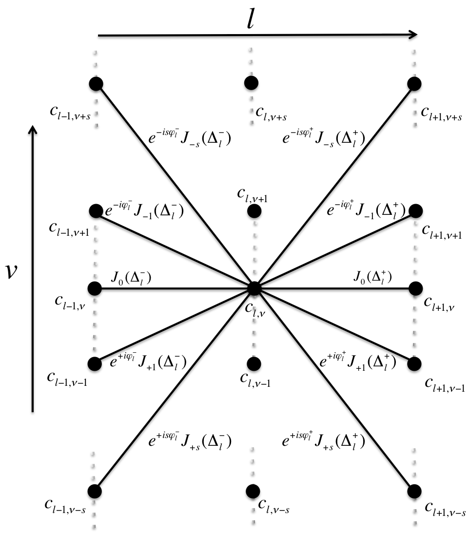
Figure 1: Two-dimensional eigenvalue problem Eq. (10). Each given site $(l,\nu)$ is connected to a set of sites $(l\pm 1,\nu-s)$ through the hopping $e^{is\phi_{l}^{\pm}}J_{s}(\Delta_{l}^{\pm})$.

This eigenvalue problem has zero hoppings along the Fourier direction $\nu$. Instead, each lattice site $c_{l,\nu}$ is connected to a number of nearest neighbor sites $c_{l\pm 1,\nu-s}$ given by the complex hopping coefficients ${\rm e}^{is\phi_{l}^{\pm}}J_{s}(\Delta_{l}^{\pm})$ (see Fig. 1). The number of strong links (connectivity) with a given site at $l,\nu$ depends on the ratio of the difference in the new onsite energies $|\epsilon_{l}-\epsilon_{l\pm 1}+s\omega|$ and the hopping strength $|J_{s}(\Delta_{l}^{\pm})|$. Strong links are then characterized by $|(\epsilon_{l}-\epsilon_{l\pm 1}+s\omega)/J_{s}(\Delta_{l}^{\pm})|\ \leq\ 1$.

III.2 Single channel vs. multi-channel regimes

In the case of zero driving strength $\mu=0$, it follows $\Delta_{l}^{\pm}=0$ for all $l$, and $J_{s}(0)=\delta_{s,0}$. The two dimensional lattice Eq.(10) turns into an infinite set of independent one-dimensional Anderson chains. For nonzero driving strength ($\mu\neq 0$) all the Floquet channels are connected. Since Watson22 ; Abramowitz72

$$J_{s}(\Delta_{l}^{\pm})\longmapsto\frac{(\Delta_{l}^{\pm})^{s}}{2^{s}s!}\ ,\quad\text{for}\ \ s\longmapsto+\infty$$ (12)

only a finite number of channels will have a nonexponentially weak hopping strength, and that number depends on the value of the argument of the Bessel functions $\Delta_{l}^{\pm}$. If for every $l$ the argument is close to zero $|\Delta_{l}^{\pm}|\leq\delta\ll 1$, it follows that $J_{0}(\Delta_{l}^{\pm})\approx 1$, and for $s\neq 0$ the Bessel functions $J_{s}(\Delta_{l}^{\pm})$ decay as Eq.(12). As a consequence Eq.(10) becomes an infinite set of uncoupled equivalent Anderson chains, and the model resembles the unperturbed case. We call this the single channel regime. This result is truly irrespective of the ratio of $\omega/W$ which controls the energy differences between connected sites. While this is evident for large frequencies $\omega\gg W$ (where the energy difference is of order $W$), it is also true in the opposite limit $\omega\ll W$ where the energy difference can be of order $\omega$ for a suitably large value of $s\sim W/\omega$, since the hoppings decay superexponentially fast with large $s$ (12).

In contrast, when $\Delta_{l}^{\pm}\geq 1$, a finite number $\mathcal{L}_{l}^{\pm}$ of the Bessel functions $J_{s}(\Delta_{l}^{\pm})$ for $s\neq 0$ are not negligible. Their typical values can be approximated as Watson22 ; Abramowitz72 :

$$J_{s}(\Delta_{l}^{\pm})\approx\sqrt{\frac{2}{\pi\Delta_{l}^{\pm}}}\cos\bigg{(}\Delta_{l}^{\pm}-\frac{s\pi}{2}-\frac{\pi}{4}\bigg{)}\ ,\quad|s|\leq\frac{\mathcal{L}_{l}^{\pm}}{2}$$ (13)

In Eq.(11), the square root of $\Delta_{l}^{\pm}$ is on the order of the disorder strength $W$. We define the parameter $\Delta$ as

$$\Delta_{l}^{\pm}\quad\longmapsto\quad\Delta=\frac{\mu W}{\omega}\ ,$$ (14)

It follows that, if $\Delta\geq 1$, the averaged number of connected channels $\mathcal{L}$ is given by

$$\mathcal{L}_{l}^{\pm}=2\Delta_{l}^{\pm}\quad\longmapsto\quad\mathcal{L}=2\Delta=\frac{2\mu W}{\omega}\ ,$$ (15)

while in Eq.(13), neglecting the cosine term that represents the Bessel function oscillation, the general value of the hopping can be approximated as

$$J_{s}\approx\sqrt{\frac{2}{\pi\Delta}}=\sqrt{\frac{2\omega}{\pi\mu W}}\ ,\quad|s|\leq\frac{\mathcal{L}}{2}$$ (16)

We call this regime the multi-channel regime. Therefore, for any given disorder and driving strengths $W$ and $\mu$, this regime will be realized in the limit of small frequencies $\omega$. This latter regime will be the focus of our investigation, since in the single channel regime the model acts similar to the undriven case.

III.3 The multi-channel regime

III.3.1 Weak driving

Let us first consider the case $\mu\ll 1$. For a given site $(l,\nu)$ there are $\mathcal{L}$ matrix elements connecting this site to a set of sites $(l+1,\nu^{\prime})$. The onsite energies of these connected sites vary in an interval $[\epsilon_{l+1}-\mu W,\epsilon_{l+1}+\mu W]$. For $\mu\ll 1$ this interval is narrow compared to $W$ which characterizes the spread of $\epsilon_{l}$. Therefore the difference in the onsite energies between two connected sites is still of the order $W$.

In general, for ladders with a finite number $N$ of equivalent Anderson chains, Dorokhov, Mello, Pereyra and Kumar Dorokhov83 ; Mello88 estimate the localization length $\zeta$ of a $N$-leg ladder as a product of the localization length $\zeta_{\mathcal{A}}$ of each leg and the number of legs $N$:

$$\zeta\sim N\cdot\zeta_{\mathcal{A}}\;.$$ (17)

The number of legs $N$ corresponds to $\mathcal{L}$. The single channel localization length can be estimated using the ratio $W_{\text{eff}}$ between the energy mismatch (disorder strength) $W$ and the matrix element $\lambda J_{s}$ from (16):

$$W_{\text{eff}}=\frac{W^{\frac{3}{2}}}{\lambda}\sqrt{\frac{\mu\pi}{2\omega}}\;.$$ (18)

We then obtain Kramer93

$$\zeta_{\mathcal{A}}(\omega)\sim\left\{\begin{array}[]{rl}\frac{100}{W_{\text{eff}}^{2}}&\text{if }\ \ W_{\text{eff}}\leq 10,\\ \frac{1}{|\ln(1/W_{\text{eff}})|}&\text{if }\ \ W_{\text{eff}}>10.\end{array}\right.$$ (19)

It follows that in the case of weak effective disorder $W_{\text{eff}}\leq 10$, the localization length $\zeta$ of our driven model is given by

$$\zeta(\omega)\sim\frac{400\lambda^{2}}{\pi W^{2}}\ \;,\;\omega\geq\frac{\mu\pi W^{3}}{200\lambda^{2}}\;.$$ (20)

The localization length $\zeta$ does not depend on the frequency $\omega$ and the driving strength $\mu$, since the increase of the number of connections $\mathcal{L}$ and the decrease of the localization length $\zeta_{\mathcal{A}}$ along each Anderson chain balance each other. Upon further decrease of the frequency $\omega$, this balancing effect is destroyed since $\Delta$ grows, the matrix element $\lambda J_{s}$ decays, and the effective disorder $W_{\text{eff}}>10$. With (19) it follows

$$\zeta(\omega)=\frac{2\mu W}{\omega}\cdot\Bigg{|}\ln\bigg{(}\frac{\lambda}{W^{\frac{3}{2}}}\sqrt{\frac{2}{\pi\mu}\omega}\bigg{)}\Bigg{|}^{-1}\;,\;\omega\leq\frac{\mu\pi W^{3}}{200\lambda^{2}}\;.$$ (21)

The localization length then diverges for $\omega\rightarrow 0$.

To summarize: in the weakly driven multichannel regime we expect a plateau in the dependence $\zeta(\omega)$ for $\omega\geq\frac{\mu\pi W^{3}}{200\lambda^{2}}$, which is replaced by a divergence for $\omega\leq\frac{\mu\pi W^{3}}{200\lambda^{2}}$.

III.3.2 Strong driving

Let us consider the case $\mu\geq 1$, and constant phases $\phi_{l}=\text{const}$. For a given site $(l,\nu)$ there are $\mathcal{L}$ matrix elements connecting this site to a set of sites $(l+1,\nu^{\prime})$. The onsite energies of these connected sites vary in an interval $[\epsilon_{l+1}-\mu W,\epsilon_{l+1}+\mu W]$. For $\mu\geq 1$ this interval is larger than $W$ which characterizes the spread of $\epsilon_{l}$. Therefore there will be typically one onsite energy amongst the connected set which is detuned by a mismatch of order $\omega$ from the one on site $(l,\nu)$. It follows that for $\mu\geq 1$ and $\omega\ll W$ we can trace a path in Eq.(10) where the onsite mismatch is of the order of the frequency $|\epsilon_{l}-\epsilon_{l\pm 1}+s\omega|\sim\omega$ and the hopping scales with the square root of the frequency $J_{s}\sim\sqrt{\omega}$ for every $l$. We call this the optimal path. The optimal path is a one dimensional random walk within the two dimensional network. Along that optimal path the localization length $\zeta_{\mathcal{OP}}$ follows from the effective disorder $W_{\text{eff}}$ between the energy mismatch (disorder strength) $\omega$ and the matrix element $\lambda J_{s}$ from (16)

$$\zeta_{\mathcal{OP}}(\omega)=\frac{100J_{\hat{s}}^{2}}{\omega^{2}}=\frac{100}{\omega^{2}}.\Bigg{(}\sqrt{\frac{2\omega}{\pi\mu W}}\Bigg{)}^{2}=\frac{200}{\pi\mu W}\frac{1}{\omega}\ .$$ (22)

For small frequencies this optimal path consists of strong links. Furthermore, paths neighboring the optimal one, are also strong links, as long as the energy detuning is not exceeding the matrix element. Since the matrix element scales with $\sqrt{\omega}$, the number of strong links diverges as $N\sim 1/\sqrt{\omega}$. Using the Dorokhov estimates, we conclude that the localization length on the network is scaling as

$$\zeta\sim\frac{200}{\pi\mu W}\frac{1}{\omega^{3/2}}\ .$$ (23)

Therefore the localization length diverges for vanishing frequency faster than in the weak driving case.

III.3.3 Local suppression of strong driving

The presence of random phases will suppress the optimal path through an increase of the minimal value of the driving strength:

$$\mu\sqrt{1+\frac{2\epsilon_{l}\epsilon_{l\pm 1}}{(\epsilon_{l}-\epsilon_{l\pm 1})^{2}}(1-\cos\theta_{l}^{\pm})}\geq 1$$ (24)

where $\theta_{l}^{\pm}=\phi_{l}-\phi_{l\pm 1}$. In particular if $\theta_{l}^{\pm}=\pi$, the square root term of Eq.(24) is equal to zero if

$$-2\epsilon_{l}\epsilon_{l\pm 1}=\epsilon_{l}^{2}+\epsilon_{l\pm 1}^{2}\quad\Leftrightarrow\quad\epsilon_{l}=-\epsilon_{l\pm 1}$$ (25)

In this case, Eq.(24) does not hold for any finite value of $\mu$ and locally between site $l$ and site $l\pm 1$ the optimal path is not accessible.

Therefore, for uncorrelated phases $\phi_{l}$, the square root term of Eq.(24) can be arbitrarily close to zero if $\theta_{l}^{\pm}\approx\pi$ and $\epsilon_{l}\approx-\epsilon_{l\pm 1}$. As a consequence, $\mu$ has to diverge to infinity in order to satisfy Eq.(24) at every step $l$ and so, for given finite values of the driving strength, the optimal path is interrupted. This will lead to a slower divergence of the localization length, which however is still expected to be faster than in the weak driving regime, since there will be finite volume parts in which the optimal path will survive.

III.3.4 Local suppression of the multi-channel regime

Since $\epsilon_{l}$ and $\phi_{l}$ are random phases, the square root term of Eq.(11) can be arbitrarily close to zero. Therefore, even deep in the multi-channel regime $\Delta\gg 1$, there might exist one or more lattice sites $l$ such that the Bessel function argument $\Delta_{l}^{\pm}\ll 1$. In that case, the hopping $J_{s}(\Delta_{l}^{\pm})\approx\delta_{s,0}$ as in the single channel regime. As a result, the multi-channel regime between site $l$ and $l\pm 1$ becomes locally suppressed.

In the case of constant phases $\phi_{l}=\text{const}$, this local suppression appears if $|\epsilon_{l}-\epsilon_{l\pm 1}|\ll\omega/\mu$.The single channel then still shows an energy difference of the order of $\omega$ or less, similar to the optimal path. For uncorrelated phases $\phi_{l}$, the probability of a local suppression of the multi-channel regime is reduced. Indeed, in order to violate the multi-channel condition $\Delta_{l}^{\pm}\gg 1$ we now need request either $|\epsilon_{l}-\epsilon_{l+1}|\ll\omega^{2}/\mu^{2}$ and $|\theta_{l}^{\pm}|\ll 1$ or $|\epsilon_{l}+\epsilon_{l+1}|\ll\omega^{2}/\mu^{2}$ and $||\theta_{l}^{\pm}|-\pi|\ll 1$.

The previously obtained estimates on the localization length $\zeta$ in either weak and strong driving regimes are therefore upper bounds.

IV Many colors

For the general case of Eq.(1), the Floquet expansion in the momentum space and the rotation of the eigenvalue problem in a basis of Bessel functions for each frequency is a natural generalization of what we have previously described in Sec.III for one color $D=1$ (see appendix). Since the frequency components of $\Omega$ are chosen to be incommensurate Eq.(2), the general form of the Floquet expansion (6) runs over the vector index ${\bf k}=(k_{1},\dots,k_{D})\in\mathbb{Z}^{D}$ Kim88 , and yields a $D+1$ dimensional time independent eigenvalue problem:

$$\begin{split}&Ec_{l,{\bf v}}=(\epsilon_{l}+\Omega\cdot{\bf v})c_{l,{\bf v}}\\ -\lambda\sum_{{\bf s}}&\Big{[}{\rm e}^{i{\bf s}\cdot\Phi_{l}^{-}}\mathcal{J}_{\bf s}^{-}c_{l-1,{\bf v}-{\bf s}}+{\rm e}^{i{\bf s}\cdot\Phi_{l}^{+}}\mathcal{J}_{\bf s}^{+}c_{l+1,{\bf v}-{\bf s}}\Big{]}\;,\end{split}$$ (26)

where ${\bf s},{\bf v}\in\mathbb{Z}^{D}$ and $\Phi_{l}^{\pm}=(\varphi_{l,i}^{\pm})_{i=1}^{D}$. The coefficients are defined as

$$\begin{split}&\tan\varphi_{l,i}^{\pm}=-\frac{\epsilon_{l\pm 1}\sin\theta_{l,i}^{\pm}}{\epsilon_{l}-\epsilon_{l\pm 1}\cos\theta_{l,i}^{\pm}}\;,\\ &\mathcal{J}_{\bf s}^{\pm}=\prod_{i=1}^{D}J_{s_{i}}\big{(}\Delta_{l,i}^{\pm}\big{)}\ ,\\ &\Delta_{l,i}^{\pm}=\frac{\mu_{i}}{\omega_{i}}\sqrt{\epsilon_{l}^{2}+\epsilon_{l\pm 1}^{2}-2\epsilon_{l}\epsilon_{l\pm 1}\cos\theta_{l,i}^{\pm}}\;,\end{split}$$ (27)

which depend on the random phase difference $\theta_{l,i}^{\pm}=\phi_{l}^{i}-\phi_{l\pm 1}^{i}$ for $i=1,\dots,D$. The resulting eigenvalue problem Eq.(26) has $D$ frequency (color) directions (with zero hopping along them) and each site $c_{l,{\bf v}}$ is connected to the nearest neighbor ones $c_{l\pm 1,{\bf v}-{\bf s}}$ through the complex matrix elements ${\rm e}^{i{\bf s}\cdot\Phi_{l}^{\pm}}\mathcal{J}_{\bf s}^{\pm}$. Each frequency color will add to the total number of channels.

Let us assume that all frequency components satisfy the same condition for single or multi-channel (either strong or weak driving) regimes. Then we conclude that the single channel regime will be applicable to multi-color driving as well, i.e. in the limit of large frequencies localization length corresponds to its value from the undriven case. In the multi-channel regime, using the above argument of Dorokhov, the localization length $\zeta_{D}$ will be of the order of $\zeta_{D}\sim D\zeta$ with $\zeta$ being the corresponding single color localization length discussed in the previous section. Therefore the localization length will stay finite for any finite number of colors. The divergence of $\zeta_{D}$ in the limit of $D\rightarrow\infty$ is in agreement with the result that a random noise driving leads to dephasing and complete delocalization Rayanov13 .

V Numerical results

We first analyze the single color driving and then discuss the two color case. We decide not to diagonalize the eigenvalue problem Eq.(7), since this will limit the required system size $N$ and the number of colors $D$. Instead, we compute the spreading of the wave packet over time for a single site excitation $\psi_{l}(t=0)=\delta_{l,N/2}$ as an initial condition using a numerical symplectic integration scheme $\text{SBAB}_{2}$ Laskar01 ; symplectic . To measure the evolution of the wave packet we calculate the second moment $m_{2}$ which, for localized modes, estimates the squared distance between the eigenmode tails. It is related to the localization length $\zeta$ of one mode as $m_{2}\sim\zeta^{2}$, and is defined as

$$m_{2}(t)=\sum_{l}\left(l-\sum_{l^{\prime}}l^{\prime}\big{|}\psi_{l^{\prime}}(t)\big{|}^{2}\right)^{2}\big{|}\psi_{l}(t)\big{|}^{2}\ .$$ (28)

Hereafter, unless indicated differently, in Eq.(1) we choose the hopping amplitude $\lambda=1$ and the disorder strength $W=4$. Furthermore, for the numerical computations we choose a system size $N=1024$ and we average $\log_{10}m_{2}(t)$ over $512$ disorder realizations, unless stated otherwise.

V.1 One color

Let us analyze the frequency dependence of the time evolution. For the weak driving case we choose the driving strength $\mu=0.1$. The multi-channel regime ($\Delta\geq 1$) is then obtained for frequencies $\omega\leq 0.4$. The time evolution of the second moment $m_{2}$ is shown in Fig. 2.

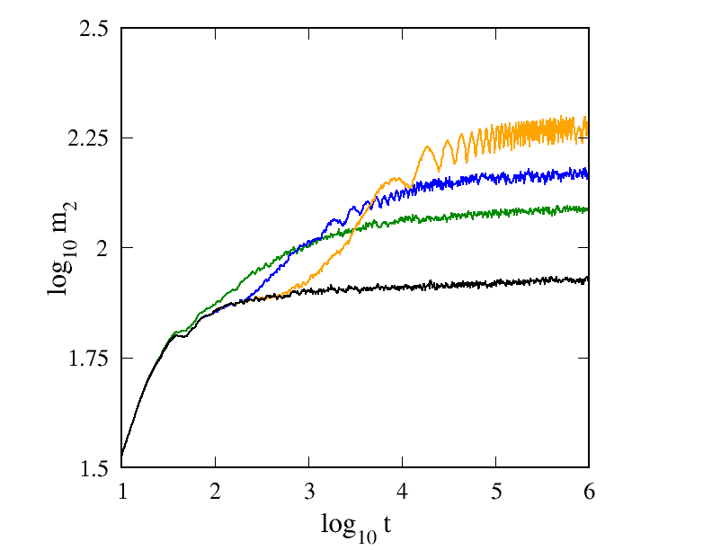
Figure 2: Time evolution of the second moment $m_{2}$ with driving strength $\mu=0.1$. Frequency values (from top to bottom at the right edge of the plot): $\omega=5\cdot 10^{-4}$ (orange), $\omega=5\cdot 10^{-3}$ (blue), $\omega=10^{-1}$ (green), undriven (black).

We observe that the second moment first increases with time, but saturates at later times, indicating a halt of spreading, and a localization of the wave packet. Therefore we conclude that there is a finite upper bound on the localization length $\zeta$ of the corresponding eigenvalue problem. The onset of spreading beyond the undriven reference curve (horizontal black one in Fig. 2) scales inversely with the driving frequency as expected.

We use the saturated value of the second moment at time $t=10^{6}$ as a measure of the squared localization length and plot it as a function of frequency $\omega$ in Fig.3 .

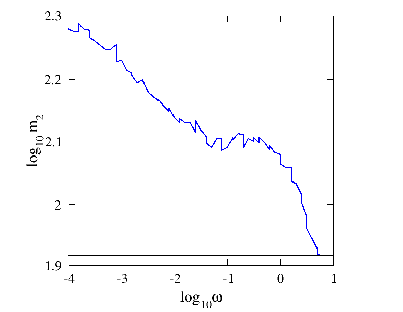
Figure 3: Saturated second moment $m_{2}$ at $t=10^{6}$ as a function of frequency $\omega$ of a one-color perturbation with $\mu=0.1$. The black horizontal line indicates the value for the undriven case.

Increasing $\omega$ in the single channel regime $\omega>0.4$ leads to a quick decay of the saturated second moment to reach the reference value of the undriven case already at $\omega\approx 4$. In the multichannel regime we observe two features: a plateau at an intermediate frequency interval, and a subsequent increase of the saturated second moment by further lowering the frequency. This is in agreement with our analytics in Sec. III.3.1.

For the strong driving regime, we consider a driving strength $\mu=1$. In Fig. 4 we plot the time evolution of the second moment $m_{2}$ for different frequencies in the multi-channel regime $\omega\leq 5$.

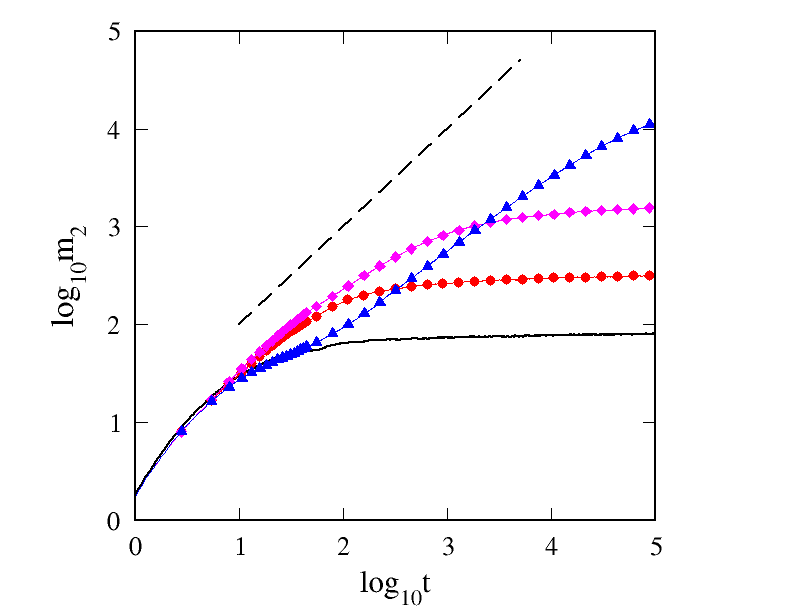
Figure 4: Time evolution of the second moment $m_{2}$ with driving strength $\mu=1$. The dashed line indicates normal diffusion $m_{2}\sim t$. Frequency values: $\omega=5$ (black), $\omega=2$ (red/circles), $\omega=0.5$ (magenta-diamonds), $\omega=0.02$ (blue-triangles).

The second moment $m_{2}$ increases as the frequency $\omega$ decreases, in agreement with Eq.(23). Moreover, we observe the appearance of transient regions of normal diffusion that extend their length as the frequency $\omega$ decreases. Again $m_{2}(t)$ saturates at larger time, indicating a halt of spreading, and a localization of the wave packet. The frequency dependence of the saturated values of the second moment $m_{2}$ is shown in Fig. 5, where we plot the second moment of the wave packet at time $t=10^{5}$ as function of the frequency $\omega$. For comparison we also replot the weak driving curve from Fig. 3.

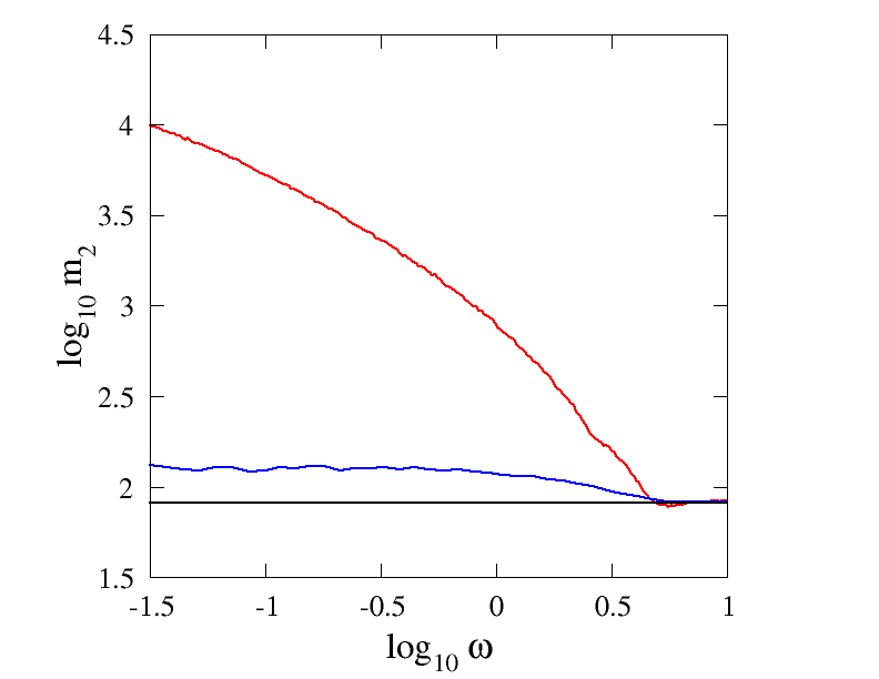
Figure 5: Saturated second moment $m_{2}$ at $t=10^{5}$ as a function of frequency $\omega$ of a one-color perturbation with $\mu=0.1$ (blue, bottom) and $\mu=1$ (red, top). The black horizontal line indicates the value of the undriven case.

Similar to the weak driving (blue curve), the second moment for the strong driving (red curve) tends to the undriven case (black horizontal line) for large frequencies and diverges for small ones. In agreement with Eq.(23), the plateau (which was observed for weak driving) is suppressed, although a reminding shoulder exists at $\omega\approx 2.5$. The strong driving yields much larger values of the saturated second moment as compared to the weak driving case, in accord with our predictions. The frequency dependence is weaker than the predicted law in Eq.(23), most likely due to the discussed local suppression of strong driving and multi-channel regimes.

In Fig. 6 we plot the time evolution of the second moment $m_{2}$ for different values of the driving strength $\mu$ in the strong driving regime. The inset of Fig. 6 shows the dependence of the saturated second moment $m_{2}$ at $t=10^{7}$ on $\mu$. We observe that the saturated moment increases up to $\mu\approx 1$ and starts to decrease for larger values of $\mu$. This subsequent decrease is qualitatively in agreement with the prediction $\zeta\sim\frac{1}{\mu}$ following from Eq.(10).

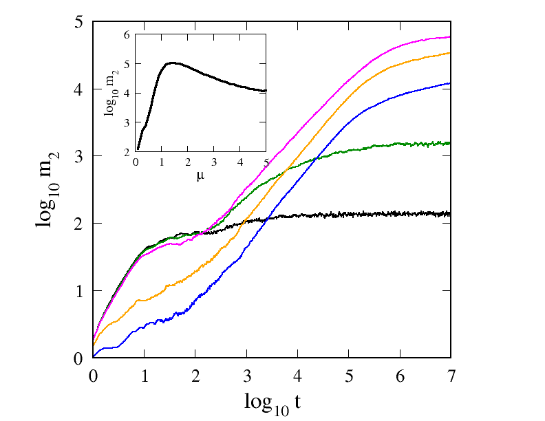
Figure 6: Time evolution of the second moment $m_{2}$ with frequency $\omega=5\cdot 10^{-3}$. Driving strength values (from top to bottom at the right edge of the plot): $\mu=1.0$ (magenta), $\mu=3.0$ (orange), $\mu=5.0$ (blue), $\mu=0.5$ (green), $\mu=0.1$ (black). The inset plot shows the dependency of the saturated second moment $m_{2}$ at $t=10^{7}$ on the drive strength. System size $N=2048$, and log₁₀m₂ is averaged over 32 disorder realizations.

V.2 Two colors

We assume the driving strengths to be equal $\mu_{1}=\mu_{2}$ and we fix the frequency relation $\omega_{2}=\sqrt{2}\omega_{1}$. We first consider the weak driving case. In Fig. 7, we compare one and two color cases for same driving strength $\mu=0.1=\mu_{1}$ and frequency $\omega=3\cdot 10^{-2}=\omega_{1}$.

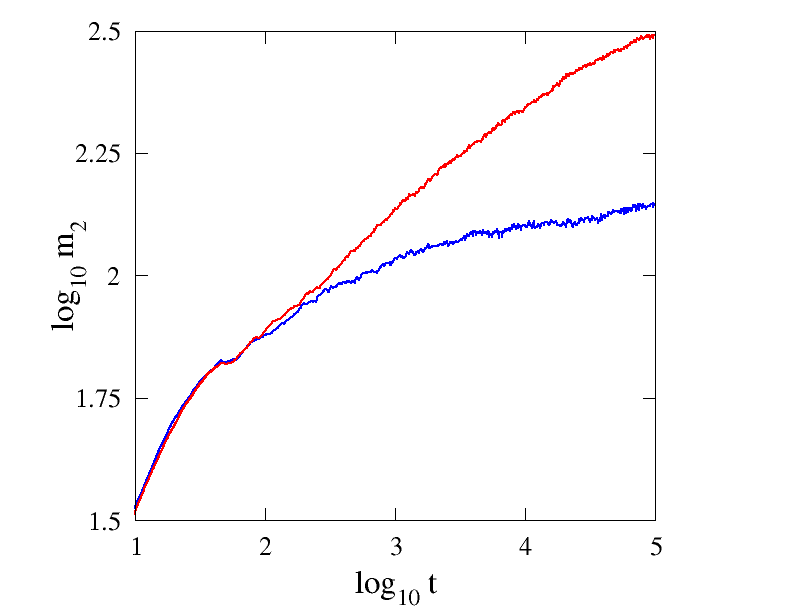
Figure 7: Time evolution of the second moment $m_{2}$ for one-color (blue, bottom) and two-color (red, top) cases with driving strength $\mu=\mu_{1}=0.1$ and frequency $\omega=\omega_{1}=3\cdot 10^{-2}$. We recall $\omega_{2}=\sqrt{2}{\omega_{1}}$ for the two color case.

The presence of a second incommensurate driving term enhances the spreading of the wave packet. However, the integration time $t=10^{5}$ is not enough to see the saturation of the second moment.

To obtain saturation at time $t=10^{5}$, we reduce the driving strength to $\mu_{1}=0.05=\mu_{2}$. In Fig.8 we plot the saturated value of the second moment $m_{2}$ at time $t=10^{5}$, as a function of the frequency $\omega_{1}$ and compare it to the weak driving single color result ($\mu=0.1$) from Fig.3.

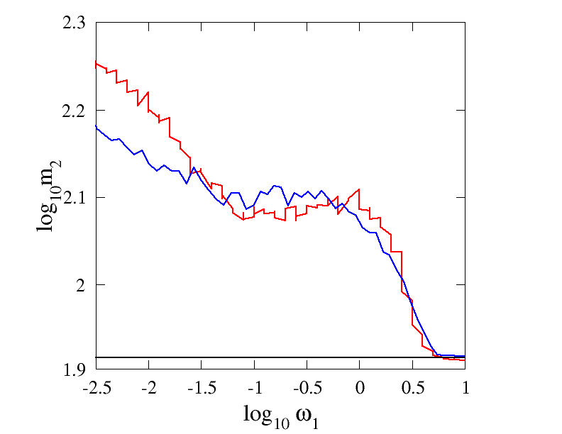
Figure 8: Saturated second moment $m_{2}$ at $t=10^{5}$ as a function of driving frequency $\omega_{1}$ with driving strengths $\mu_{1}=\mu_{2}=0.05$ (red curve, top at left corner). The blue curve corrsponds to the single color one from Fig.3. We recall $\omega_{2}=\sqrt{2}{\omega_{1}}$. The black horizontal line indicates the value of the undriven case.

The values approach the undriven case (black horizontal line) for approximately $\omega_{1}\geq 4$, in good agreement with the single channel regime $\omega_{1},\omega_{2}\geq 2$. Similar to the one color case, the saturated second moment exhibits a plateau in the multi-channel regime. Notably the height of the plateau is practically equal to the single color one reported in Fig.3, in full accord with our estimate of the localization length in Eq.(20), which is independent of the driving strength $\mu$ and more general independent of the number of participating channels. Therefore the presence of a second frequency which increases the number of channels, should not change the plateau value, as observed.

For the strong driving case, we consider $\mu_{1}=\mu_{2}=1$. In Fig. 9 we show the time evolution of the second moment $m_{2}$ for frequencies $\omega_{1,2}$ chosen in the multi-channel regime.

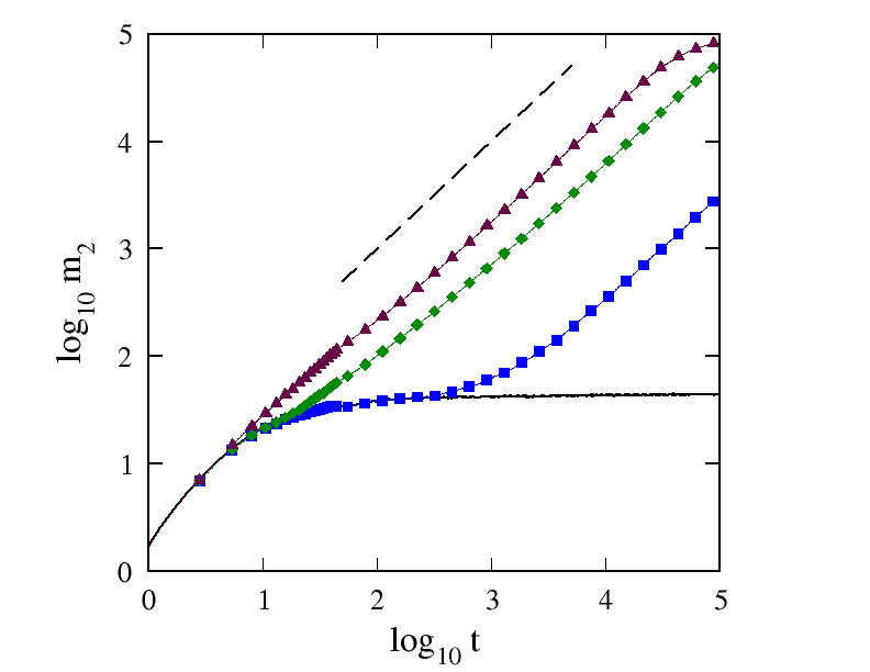
Figure 9: Time evolution of the second moment $m_{2}$ with driving strength $\mu_{1}=\mu_{2}=1$. We recall $\omega_{2}=\sqrt{2}{\omega_{1}}$. The dashed line indicates normal diffusion $m_{2}\sim t$. Frequency values: $\omega_{1}=5\cdot 10^{-1}$ (maroon/triangles), $\omega_{1}=5\cdot 10^{-2}$ (green/diamonds), $\omega_{1}=5\cdot 10^{-4}$ (blue/squares), undriven (black).

We observe long lasting transient regions of diffusive spreading, with a subsequent halt and localization. We also observe a significant increase in the localization length as compared to the single color case, in agreement with our predictions.

VI Summary and Conclusions

In this work we have studied the spreading of a wave packet for a one-dimensional disordered chain in the presence of a multi-frequency quasi-periodic drive. For each term (color) of the driving, the Floquet representation is used to arrive at a time-independent eigenvalue problem on a two-dimensional lattice, with one direction corresponding to the original spatial extension, and the second one to the Floquet (driving) one. We transform into a Wannier-Stark basis which is diagonal along the Floquet direction, and analyze the resulting eigenvalue problem. For large driving frequencies the equations reduce to uncoupled single channel ones, which are essentially equivalent to the undriven case. For small driving frequencies we obtain a multi-channel regime with a substantial increase of the localization length, and its divergence in the limit of vanishing frequency. This multi-channel regime divides into two further regimes of weak and strong driving amplitudes, which yield different scaling laws.

In the many colors case, we have shown that each incommensurate color is independent from the others and can be treated separately. The localization length of the model will then be proportional to the single color localization length, and scales with the number of colors set in the multi-channel regime. Therefore, it will remain finite for any finite number of colors.

Numerically we have observed that in the strong driving, the model exhibit transient regions of diffusive dynamics before localization occurs. The localization volume increases as the number of colors increases, when satisfying the multi-channel regime condition. It follows that for $D\rightarrow\infty$, the localization length will diverge to infinity and the region of diffusive dynamics will extend to infinity until a complete delocalization is observed. The divergence of the number of colors $D$ corresponds to the loss of quasiperiodicity of the driving term, and consequently to an effective random driving which leads to a loss of Anderson localization in that limit.

Mathematical studies of the single color $D=1$ case Soffer03 and multicolor case $D>1$ Bourgain04 predict stability of Anderson localization in the regime of strong disorder. These results are in line with our findings, since the limit of strong disorder is corresponding to the single channel regime, which is essentially independent on the number of colors, with a localization length close to the one of the undriven case.

*

Appendix A Floquet analysis and coordinate transformation

We focus on the one color case $D=1$ using references Watson22 ; Abramowitz72 . The $D$ color case is a generalization of these calculations. The one-dimensional time-dependent model Eq.(3) is mapped to a time independent two-dimensional eigenvalue problem Eq.(7) via the Floquet expansion Eq.(4)

$$\psi_{l}(t)=\sum_{k}A_{l,k}e^{-i[(E-k\omega)t-k\phi_{l}]}\;.$$ (29)

With

$$\begin{split}&\quad\mu\epsilon_{l}\cos(\omega t+\phi_{l})\psi_{l}=\\ &=\frac{\mu\epsilon_{l}}{2}\sum_{k}\big{[}A_{l,k-1}+A_{l,k+1}\big{]}e^{-i[(E-k\omega)t-k\phi_{l}]}\end{split}$$ (30)

and

$$\begin{split}&\quad\lambda(\psi_{l+1}+\psi_{l-1})=\\ &=\lambda\sum_{k}\Big{[}A_{l-1,k}e^{-i[(E-k\omega)t-k\phi_{l-1}]}\\ &\qquad\quad+A_{l-1,k}e^{-i[(E-k\omega)t-k\phi_{l-1}]}\Big{]}\\ &-\lambda\sum_{k}\Big{[}A_{l-1,k}e^{-ik(\phi_{l}-\phi_{l-1})}e^{-i[(E-k\omega)t-k\phi_{l}]}\\ &\qquad\quad+A_{l+1,k}e^{-ik(\phi_{l}-\phi_{l+1})}e^{-i[(E-k\omega)t-k\phi_{l}]}\Big{]}\ \end{split}$$ (31)

we define the hopping coefficients $\xi_{l,k}^{\pm}$ as

$$\xi_{l,k}^{\pm}=e^{-ik(\phi_{l}-\phi_{l\pm 1})}$$ (32)

to arrive at

$$\begin{split}&\quad\sum_{k}(E-k\omega)A_{l,k}e^{-i[(E-k\omega)t-k\phi_{l}]}=\\ &=\sum_{k}\bigg{[}\epsilon_{l}A_{l,k}+\frac{\mu\epsilon_{l}}{2}\big{(}A_{l,k-1}+A_{l,k+1}\big{)}\\ &\qquad-\lambda\big{(}\xi_{l,k}^{-}A_{l-1,k}+\xi_{l,k}^{+}A_{l+1,k}\big{)}\bigg{]}e^{-i[(E-k\omega)t-k\phi_{l}]}\\ \end{split}$$ (33)

which finally yields the two dimensional eigenvalue problem of Eq.(7)

$$\begin{split}EA_{l,k}&=(\epsilon_{l}+k\omega)A_{l,k}-\lambda(\xi_{l,k}^{-}A_{l-1,k}+\xi_{l,k}^{+}A_{l+1,k})\\ &+\frac{\mu\epsilon_{l}}{2}\big{(}A_{l,k-1}+A_{l,k+1}\big{)}\ .\end{split}$$ (34)

This is then transformed using Eq.(6):

$$A_{l,k}=\sum_{\nu}c_{l,\nu}B_{l,k}^{(\nu)}\ ,\qquad B_{l,k}^{(\nu)}=J_{k-\nu}\bigg{(}\frac{\mu\epsilon_{l}}{\omega}\bigg{)}\ .$$ (35)

The basis $\mathcal{B}=\{B_{l,k}^{(\nu)}\}_{\nu}$ diagonalizes the eigenvalue problem in the Fourier direction $k$ with eigenvalues $\epsilon_{\nu}=\omega\nu$. It follows that

$$\begin{split}&\quad k\omega A_{l,k}+\frac{\mu\epsilon_{l}}{2}\big{(}A_{l,k-1}+A_{l,k+1}\big{)}=\\ &=\sum_{\nu}c_{l,\nu}\bigg{[}k\omega B_{l,k}^{(\nu)}+\frac{\mu\epsilon_{l}}{2}\Big{(}B_{l,k-1}^{(\nu)}+B_{l,k+1}^{(\nu)}\Big{)}\bigg{]}\\ &=\sum_{\nu}\omega\nu\ c_{l,\nu}B_{l,k}^{(\nu)}\;.\end{split}$$ (36)

The eigenvalue problem Eq.(34) in the new basis $\mathcal{B}$ reads

$$\begin{split}E\sum_{\nu}&c_{l,\nu}B_{l,k}^{(\nu)}=\sum_{\nu}\Big{[}(\epsilon_{l}+\omega\nu)c_{l,\nu}B_{l,k}^{(\nu)}\\ &-\lambda\big{(}\xi_{l,k}^{-}c_{l-1,\nu}B_{l-1,k}^{(\nu)}+\xi_{l,k}^{+}c_{l+1,\nu}B_{l+1,k}^{(\nu)}\big{)}\Big{]}\ .\end{split}$$ (37)

We multiply both sides of Eq.(37) with a second Bessel function $B_{l,k}^{(\nu_{2})}$ of index $\nu_{2}$ and then sum over $k$. Using the Bessel functions orthonormality relation Watson22 ; Abramowitz72

$$\sum_{k}B_{l,k}^{(\nu)}B_{l,k}^{(\nu_{2})}=\sum_{k}J_{k-\nu}\bigg{(}\frac{\mu\epsilon_{l}}{\omega}\bigg{)}J_{k-\nu_{2}}\bigg{(}\frac{\mu\epsilon_{l}}{\omega}\bigg{)}=\delta_{\nu,\nu_{2}}$$ (38)

in Eq.(37) we obtain

$$\begin{split}&\qquad\quad E\sum_{k}\sum_{\nu}c_{l,\nu}B_{l,k}^{(\nu)}B_{l,k}^{(\nu_{2})}=Ec_{l,\nu}\ ,\\ &\sum_{k}\sum_{\nu}(\epsilon_{l}+\omega\nu)c_{l,\nu}B_{l,k}^{(\nu)}B_{l,k}^{(\nu_{2})}=(\epsilon_{l}+\omega\nu)c_{l,\nu}\ .\end{split}$$ (39)

The matrix elements (hopping) along the real direction $l$ become

$$\begin{split}&\quad\sum_{k}\sum_{\nu}\xi_{l,k}^{\pm}c_{l\pm 1,\nu}B_{l\pm 1,k}^{(\nu)}B_{l,k}^{(\nu_{2})}=\\ &=\sum_{\nu}c_{l\pm 1,\nu}\bigg{(}\sum_{k}\xi_{l,k}^{\pm}B_{l\pm 1,k}^{(\nu)}B_{l,k}^{(\nu_{2})}\bigg{)}\;.\end{split}$$ (40)

Using Graf’s generalization of Neumann’s addition theorem Watson22 ; Abramowitz72

$$\begin{split}\sum_{k}&e^{ik\theta}J_{\nu+k}(x)J_{k}(y)=\\ &=\bigg{(}\frac{x-ye^{-i\theta}}{x-ye^{i\theta}}\bigg{)}^{\frac{\nu}{2}}J_{\nu}\Big{(}\sqrt{x^{2}+y^{2}-2xy\cos\theta}\Big{)}\;.\end{split}$$ (41)

and defining the random phase difference

$$\theta_{l}^{\pm}=\phi_{l}-\phi_{l\pm 1}\ ,$$ (42)

Eq.(40) is modified as

$$\begin{split}&\sum_{k}\sum_{\nu}\xi_{l,k}^{\pm}c_{l\pm 1,\nu}B_{l\pm 1,k}^{(\nu)}B_{l,k}^{(\nu_{2})}=\sum_{s}\big{(}\sigma_{l}^{\pm}\big{)}^{s}J_{s}\big{(}\Delta_{l}^{\pm}\big{)}c_{l\pm 1,\nu-s}\end{split}$$ (43)

where

$$\begin{split}\sigma_{l}^{\pm}&=\Bigg{(}\frac{\epsilon_{l}-e^{-i\theta_{l}^{\pm}}\epsilon_{l\pm 1}}{\epsilon_{l}-e^{i\theta_{l}^{\pm}}\epsilon_{l\pm 1}}\Bigg{)}^{\frac{1}{2}}\;,\\ \Delta_{l}^{\pm}&=\frac{\mu}{\omega}\sqrt{\epsilon_{l}^{2}+\epsilon_{l\pm 1}^{2}-2\epsilon_{l}\epsilon_{l\pm 1}\cos\theta_{l}^{\pm}}\;.\end{split}$$ (44)

Since the complex coefficient $\sigma_{l}^{\pm}$ has absolute value equal to unity, we rewrite it as

$$\begin{split}&\sigma_{l}^{\pm}={\rm e}^{i\varphi_{l}^{\pm}}\ ,\qquad\tan\varphi_{l}^{\pm}=-\frac{\epsilon_{l\pm 1}\sin\theta_{l}^{\pm}}{\epsilon_{l}-\epsilon_{l\pm 1}\cos\theta_{l}^{\pm}}\;.\end{split}$$ (45)

The final eigenvalue problem becomes (Eq.(10))

$$\begin{split}&Ec_{l,\nu}=(\epsilon_{l}+\omega\nu)c_{l,\nu}\\ -\lambda\sum_{s}\Big{[}&{\rm e}^{is\varphi_{l}^{-}}J_{s}\big{(}\Delta_{l}^{-}\big{)}c_{l-1,\nu-s}+{\rm e}^{is\varphi_{l}^{+}}J_{s}\big{(}\Delta_{l}^{+}\big{)}c_{l+1,\nu-s}\Big{]}\;.\end{split}$$ (46)

References

- (1) P.W. Anderson, Phys. Rev. 109, 1492 (1958).
- (2) E. Abrahams, P. W. Anderson, D. C. Licciardello, and T. V. Ramakrishnan, Phys. Rev. Lett. 42, 673 (1979).
- (3) B.R. Bulka, B. Kramer and A. MacKinnon, Zeitschrift für Physik B Condensed Matter, 60, 1, 13-17 (1985).
- (4) Y. Lahini, A. Avidan, F. Pozzi, M. Sorel, R. Morandotti, D.N. Christodoulides and Y. Silberberg, Phys. Rev. Lett. 100, 013906 (2008)
- (5) J. Billy, V. Josse, Z. Zuo, A. Bernard, B. Hambrecht, P. Lugan, D. Clément, L. Sanchez-Palencia, P. Bouyer and A. Aspect, Nature 453, 891-894 (2008).
- (6) G. Roati, C. D’Errico, L. Fallani, M. Fattori, C. Fort, M. Zaccanti, G. Modugno, M. Modugno and M. Inguscio, Nature 453, 895-898 (2008).
- (7) K. Rayanov, G. Radons and S. Flach, Phys. Rev. E 88 012901 (2013).
- (8) H. Yamada, K. S. Ikeda, and M. Goda, Phys. Lett. A 182, 77 (1993).
- (9) H. Yamada, and K. S. Ikeda, Phys. Lett. A 248, 179 (1998).
- (10) H. Yamada, and K. S. Ikeda, Phys. Rev. E 59, 5214 (1999).
- (11) D.F. Martinez, and R.A. Molina, Phys. Rev. B 73, 073104 (2006).
- (12) T. Kitagawa,T. Oka, and E. Demler, Ann. Phys. 327, 1868 (2012).
- (13) B. Kramer and A. MacKinnon, Rep. Prog. Phys. 56, 1469 (1993).
- (14) G. Floquet, Annales scientifiques De l’ENS, 12, second edition, 47 (1883).
- (15) J. H. Shirley, Phys. Rev. 138, B979 (1965).
- (16) H. Fukuyama, R. A. Bari, and H. C. Fogedby, Phys. Rev. B 8, 5579 (1973).
- (17) D. O. Krimer, R. Khomeriki and S. Flach, Phys. Rev. E 80, 036201 (2009).
- (18) G.N. Watson, A Treatise on the Theory of Bessel function, Cambridge University press (1922).
- (19) M. Abramowitz and I. A. Stegun, Handbook of Mathematical Functions, Dover Publications Inc., New York (1972).
- (20) O. N. Dorokhov, Solid State Commun. 46, 605 (1983).
- (21) P. A. Mello, P. Pereyra and N. Kummar, Ann. Phys. 181, 290 (1988).
- (22) S. Kim, S. Ostlund and G. Yu, Physica D 31 117-126 (1988).
- (23) J. Laskar, and P. Robutel, Celest. Mech. Dyn. Astron. 80, 39 (2001).
- (24) Ch. Skokos, E. Gerlach, J.D. Bodyfelt, G. Papamikos and S. Eggl, Phys. Lett. A 378 1809 (2014); E. Gerlach, S. Eggl, Ch. Skokos, J.D. Bodyfelt and G. Papamikos, Proc. of 10th HSTAM Intnl. Congress on Mechanics (2013); E. Gerlach, J. Meichsner and Ch. Skokos, arXiv:1512.07778.
- (25) A. Soffer,and W. Wang, Commun. Part. Diff. Eq. 28, 333 (2003).
- (26) J. Bourgain,and W. Wang, Commun. Math. Phys. 248, 429 (2004).