Loss factorization, weakly supervised learning
and label noise robustness

Giorgio Patrini
Australian National University, NICTA
giorgio.patrini@anu.edu.au
   Frank Nielsen
École Polytechnique, Sony Computer Science Laboratories Inc.
nielsen@lix.polytechnique.fr
   Richard Nock
NICTA, Australian National University
richard.nock@nicta.com.au
   Marcello Carioni
Max Planck Institute for Mathematics in the Sciences
marcello.carioni@mis.mpg.de
Abstract

We prove that the empirical risk of most well-known loss functions factors into a linear term aggregating all labels with a term that is label free, and can further be expressed by sums of the loss. This holds true even for non-smooth, non-convex losses and in any rkhs. The first term is a (kernel) mean operator –the focal quantity of this work– which we characterize as the sufficient statistic for the labels. The result tightens known generalization bounds and sheds new light on their interpretation.

Factorization has a direct application on weakly supervised learning. In particular, we demonstrate that algorithms like sgd and proximal methods can be adapted with minimal effort to handle weak supervision, once the mean operator has been estimated. We apply this idea to learning with asymmetric noisy labels, connecting and extending prior work. Furthermore, we show that most losses enjoy a data-dependent (by the mean operator) form of noise robustness, in contrast with known negative results.

1 Introduction

Supervised learning is by far the most effective application of the machine learning paradigm. However, there is a growing need of decoupling the success of the field from its topmost framework, often unrealistic in practice. In fact while the amount of available data grows continuously, its relative training labels –often derived by human effort– become rare, and hence learning is performed with partially missing, aggregate-level and/or noisy labels. For this reason, weakly supervised learning (wsl) has attracted much research. In this work, we focus on binary classification under weak supervision. Traditionally, wsl problems are attacked by designing ad-hoc loss functions and optimization algorithms tied to the particular learning setting. Instead, we advocate to “do not reinvent the wheel” and present an unifying treatment. In summary, we show that, under a mild decomposability assumption,

Any loss admitting a minimizing algorithm over fully labelled data, can also be minimized in wsl setting with provable generalization and noise robustness guarantees. Our proof is constructive: we show that a simple change in the input and of one line of code is sufficient.
Refer to caption
(a) logistic loss
Refer to caption
(b) square loss
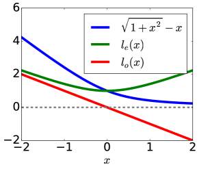
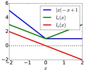
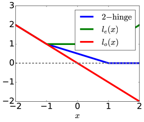
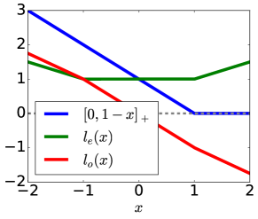
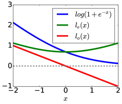
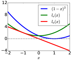
Figure 1: Loss factorization: l(x)=le(x)+lo(x)𝑙𝑥subscript𝑙𝑒𝑥subscript𝑙𝑜𝑥l(x)=l_{e}(x)+l_{o}(x).

1.1 Contribution and related work

We introduce linear-odd losses (lols), a definition that not does demand smoothness or convexity, but that a loss l𝑙l is such that l(x)l(x)𝑙𝑥𝑙𝑥l(x)-l(-x) is linear. Many losses of practical interest are such, e.g. logistic and square. We prove a theorem reminiscent of Fisher-Neyman’s factorization (Lehmann and Casella, 1998) of the exponential family which lays the foundation of this work: it shows how empirical l𝑙l-risk factors (Figure 1) in a label free term with another incorporating a sufficient statistic of the labels, the mean operator. The interplay of the two components is still apparent on newly derived generalization bounds, that also improve on known ones (Kakade et al., 2009). Aside from factorization, the above linearity is known to guarantee convexity to certain losses used in learning on positive and unlabeled data (pu) in the recent (du Plessis et al., 2015).

An advantage of isolating labels comes from applications on wsl. In this scenario, training labels are only partially observable due to an unknown noise process (Garcıa-Garcıa and Williamson, 2011; Hernandez-Gonzalez et al., 2016). For example, labels may be noisy (Natarajan et al., 2013), missing as with semi-supervision (Chapelle et al., 2006) and pu (du Plessis et al., 2015), or aggregated as it happens in multiple instance learning (Dietterich et al., 1997) and learning from label proportions (llp) (Quadrianto et al., 2009). As the success of those areas shows, labels are not strictly needed for learning. However, most wsl methods implicitly assumes that labels must be recovered in training, as pointed out by (Joulin and Bach, 2012). Instead, sufficiency supports a more principled two-step approach: (1) estimate the mean operator from weakly supervised data and (2) plug it into any lol and resort to known procedures for empirical risk minimization (erm). Thus, (1) becomes the only technical obstacle in adapting an algorithm, although often easy to surpass. Indeed, this approach unifies a growing body of literature (Quadrianto et al., 2009; Patrini et al., 2014; van Rooyen et al., 2015; Gao et al., 2016). As a showcase, we implement (2) by adapting stochastic gradient descent (sgd) to wsl. The upgrade only require to transform input by a “double sample trick” and to sum the mean operator in the model update.

Finally, we concentrate on learning with asymmetric label noise. We connect and extend previous work of (Natarajan et al., 2013; van Rooyen et al., 2015) by designing an unbiased mean operator estimator, for which we derive generalization bounds independent on the chosen lol and algorithm. Recent results (Long and Servedio, 2010) have shown that requiring the strongest form of robustness –on any possible noisy sample– rules out most losses commonly used, and have drifted research focus on non-convex (Stempfel and Ralaivola, 2009; Masnadi-Shirazi et al., 2010; Ding and Vishwanathan, 2010) or linear losses (van Rooyen et al., 2015). Our approach is more pragmatic, as we show that any lols enjoy an approximate form of noise robustness which converges, on a data-dependent basis, to the strongest one. The mean operator is still central here, being the data-dependent quantity that shapes the bound. The theory is validated with experimental analysis, for which we call the adapted sgd as a black box.

Elements of this work appeared in an early version (Patrini et al., 2015), mostly interested in elucidating the connection between loss factorization and α𝛼\alpha-label differential privacy (Chaudhuri and Hsu, 2011).

Next, Section 2 settles notations and background. Section 3 states the Factorization Theorem. Sections 4 and 5 focus on wsl and noisy labels. Section 6 discusses the paper. Proofs and additional results are given in Appendix.

2 Learning setting and background

We denote vectors in bold as 𝒙𝒙\bm{x} and 1{p}1𝑝1\{p\} the indicator of p𝑝p being true. We define [m]=.{1,,m}superscript.delimited-[]𝑚1𝑚[m]\stackrel{{\scriptstyle\mathrm{.}}}{{=}}\{1,\dots,m\} and [x]+=.max(0,x)superscript.subscriptdelimited-[]𝑥0𝑥[x]_{+}\stackrel{{\scriptstyle\mathrm{.}}}{{=}}\max(0,x). In binary classification, a learning sample 𝒮={(𝒙i,yi),i[m]}𝒮subscript𝒙𝑖subscript𝑦𝑖𝑖delimited-[]𝑚\mathcal{S}=\{(\bm{x}_{i},y_{i}),i\in[m]\} is a sequence of (observation, label) pairs, the examples, drawn from an unknown distribution 𝒟𝒟\mathcal{D} over 𝒳×𝒴𝒳𝒴\mathcal{X}\times\mathcal{Y}, with 𝒳d𝒳superscript𝑑\mathcal{X}\subseteq\mathbb{R}^{d} and 𝒴={1,1}𝒴11\mathcal{Y}=\{-1,1\}. Expectation (or average) over (𝒙,y)𝒟similar-to𝒙𝑦𝒟(\bm{x},y)\sim\mathcal{D} (𝒮𝒮\mathcal{S}) is denoted as 𝔼𝒟subscript𝔼𝒟\mathbb{E}_{\mathcal{D}} (𝔼𝒮subscript𝔼𝒮\mathbb{E}_{\mathcal{S}}).

Given a hypothesis h,h:𝒳:𝒳h\in\mathcal{H},h:\mathcal{X}\rightarrow\mathbb{R}, a loss is any function l:𝒴×:𝑙𝒴l:\mathcal{Y}\times\mathbb{R}\rightarrow\mathbb{R}. A loss gives a penalty l(y,h(𝒙))𝑙𝑦𝒙l(y,h(\bm{x})) when predicting the value h(𝒙)𝒙h(\bm{x}) and the observed label is y𝑦y. We consider margin losses, i.e. l(y,h(𝒙))=l(yh(𝒙))𝑙𝑦𝒙𝑙𝑦𝒙l(y,h(\bm{x}))=l(yh(\bm{x})) (Reid and Williamson, 2010), which are implicitly symmetric: l(yh(𝒙))=l(y(h(𝒙)))𝑙𝑦𝒙𝑙𝑦𝒙l(yh(\bm{x}))=l(-y\cdot(-h(\bm{x}))). For notational convenience, we will often use a generic scalar argument l(x)𝑙𝑥l(x). Examples are 010101 loss 1{x<0}1𝑥01\{x<0\}, logistic loss log(1+ex)1superscript𝑒𝑥\log(1+e^{-x}), square loss (1x)2superscript1𝑥2(1-x)^{2} and hinge loss [1x]+subscriptdelimited-[]1𝑥[1-x]_{+}.

The goal of binary classification is to select a hypothesis hh\in\mathcal{H} that generalizes on 𝒟𝒟\mathcal{D}. That is, we aim to minimize the true risk on the 010101 loss R𝒟,01(h)=.𝔼𝒟[1{yh(𝒙)<0}]superscript.subscript𝑅𝒟01subscript𝔼𝒟delimited-[]1𝑦𝒙0R_{\mathcal{D},01}(h)\stackrel{{\scriptstyle\mathrm{.}}}{{=}}\mathbb{E}_{\mathcal{D}}[1\{yh(\bm{x})<0\}]. In practice, we only learn from a finite learning sample 𝒮𝒮\mathcal{S} and thus minimize the empirical l𝑙l-risk R𝒮,l(h)=.𝔼𝒮[l(yh(𝒙))]=1mi[m]l(yih(𝒙i))superscript.subscript𝑅𝒮𝑙subscript𝔼𝒮delimited-[]𝑙𝑦𝒙1𝑚subscript𝑖delimited-[]𝑚𝑙subscript𝑦𝑖subscript𝒙𝑖R_{\mathcal{S},l}(h)\stackrel{{\scriptstyle\mathrm{.}}}{{=}}\mathbb{E}_{\mathcal{S}}[l(yh(\bm{x}))]=\frac{1}{m}\sum_{i\in[m]}l(y_{i}h(\bm{x}_{i})), where l𝑙l is a tractable upperbound of 010101 loss.

Finally, we discuss the meaning of wsl –and in particular of weakly supervised binary classification. The difference with the above is at training time: we learn on a sample 𝒮~~𝒮\tilde{\mathcal{S}} drawn from a noisy distribution 𝒟~~𝒟\tilde{\mathcal{D}} that may flip, aggregate or suppress labels, while observations are the same. Still, the purpose of learning is unchanged: to minimize the true risk. A rigorous definition will not be relevant in our study.

2.1 Background: exponential family and logistic loss

Some background on the exponential family is to come. We can learn a binary classifier fitting a model in the conditional exponential family parametrized by 𝜽𝜽\bm{\theta}: p𝜽(y|𝒙)=exp(𝜽,y𝒙logy𝒴exp𝜽,y𝒙)subscript𝑝𝜽conditional𝑦𝒙𝜽𝑦𝒙subscript𝑦𝒴𝜽𝑦𝒙p_{\bm{\theta}}(y|\bm{x})=\exp(\langle\bm{\theta},y\bm{x}\rangle-\log\sum_{y\in\mathcal{Y}}\exp\langle\bm{\theta},y\bm{x}\rangle), with y𝑦y random variable. The two terms in the exponent are the log-partition function and the sufficient statistic yi𝒙isubscript𝑦𝑖subscript𝒙𝑖y_{i}\bm{x}_{i}, which fully summarizes one example (𝒙,y)𝒙𝑦(\bm{x},y). The Fisher-Neyman theorem (Lehmann and Casella, 1998, Theorem 6.5) gives a sufficient and necessary condition for sufficiency of a statistic T(y)𝑇𝑦T(y): the probability distribution factors in two functions, such that 𝜽𝜽{\bm{\theta}} interacts with the y𝑦y only through T𝑇T:

p𝜽(y)=g𝜽(T(y))g(y).subscript𝑝𝜽𝑦subscript𝑔𝜽𝑇𝑦superscript𝑔𝑦p_{\bm{\theta}}(y)=g_{\bm{\theta}}(T(y))g^{\prime}(y)\>\>.

In our case, it holds that g(y|𝒙)=1superscript𝑔conditional𝑦𝒙1g^{\prime}(y|\bm{x})=1, T(y|𝒙)=y𝒙𝑇conditional𝑦𝒙𝑦𝒙T(y|\bm{x})=y\bm{x} and g𝜽(|𝒙)=exp(𝜽,logy𝒴exp(𝜽,y𝒙)g_{\bm{\theta}}(\cdot|\bm{x})=\exp(\langle\bm{\theta},\cdot\rangle\ -\log\sum_{y\in\mathcal{Y}}\exp(\langle\bm{\theta},y\bm{x}\rangle), since the value of y𝑦y is not needed to compute g𝜽subscript𝑔𝜽g_{\bm{\theta}}. This shows how y𝒙𝑦𝒙y\bm{x} is indeed sufficient (for y𝑦y). Now, under the i.i.d. assumption, the log-likelihood of 𝜽𝜽\bm{\theta} is (the negative of)

i=1mlogy𝒴ey𝜽,𝒙ii=1m𝜽,yi𝒙isuperscriptsubscript𝑖1𝑚subscript𝑦𝒴superscript𝑒𝑦𝜽subscript𝒙𝑖superscriptsubscript𝑖1𝑚𝜽subscript𝑦𝑖subscript𝒙𝑖\displaystyle\sum_{i=1}^{m}\log\sum_{y\in\mathcal{Y}}e^{y\langle\bm{\theta},\bm{x}_{i}\rangle}-\sum_{i=1}^{m}\langle\bm{\theta},y_{i}\bm{x}_{i}\rangle (1)
=i=1mlogy𝒴ey𝜽,𝒙ii=1mlogeyi𝜽,𝒙iabsentsuperscriptsubscript𝑖1𝑚subscript𝑦𝒴superscript𝑒𝑦𝜽subscript𝒙𝑖superscriptsubscript𝑖1𝑚superscript𝑒subscript𝑦𝑖𝜽subscript𝒙𝑖\displaystyle=\sum_{i=1}^{m}\log\sum_{y\in\mathcal{Y}}e^{y\langle\bm{\theta},\bm{x}_{i}\rangle}-\sum_{i=1}^{m}\log e^{y_{i}\langle\bm{\theta},\bm{x}_{i}\rangle}
=i=1mlog(e𝜽,𝒙i+e𝜽,𝒙ieyi𝜽,𝒙i)absentsuperscriptsubscript𝑖1𝑚superscript𝑒𝜽subscript𝒙𝑖superscript𝑒𝜽subscript𝒙𝑖superscript𝑒subscript𝑦𝑖𝜽subscript𝒙𝑖\displaystyle=\sum_{i=1}^{m}\log\left(\frac{e^{\langle\bm{\theta},\bm{x}_{i}\rangle}+e^{-\langle\bm{\theta},\bm{x}_{i}\rangle}}{e^{y_{i}\langle\bm{\theta},\bm{x}_{i}\rangle}}\right)
=i=1mlog(1+e2yi𝜽,𝒙i).absentsuperscriptsubscript𝑖1𝑚1superscript𝑒2subscript𝑦𝑖𝜽subscript𝒙𝑖\displaystyle=\sum_{i=1}^{m}\log\left(1+e^{-2y_{i}\langle\bm{\theta},\bm{x}_{i}\rangle}\right)\>\>. (2)

Step (2) is true because y𝒴𝑦𝒴y\in\mathcal{Y}. At last, by At last, by re-parameterizing 𝜽𝜽\bm{\theta} and normalizing, we obtain the empirical risk of logistic loss. Equation (1) shows how the loss splits into a linear term aggregating the labels and another, label free term. We translate this property for classification with erm, by transferring the ideas of sufficiency and factorization to a wide set of losses including the ones of (Patrini et al., 2014).

3 Loss factorization and sufficiency

The linear term just encountered in logistic loss integrates a well-studied statistical object.

Definition 1

The (empirical) mean operator of a learning sample 𝒮𝒮\mathcal{S} is 𝛍𝒮=.𝔼𝒮[y𝐱].superscript.subscript𝛍𝒮subscript𝔼𝒮delimited-[]𝑦𝐱\bm{\mu}_{\mathcal{S}}\stackrel{{\scriptstyle\mathrm{.}}}{{=}}\mathbb{E}_{\mathcal{S}}\left[y\bm{x}\right]\>\>.

We drop the 𝒮𝒮\mathcal{S} when clear by the context. The name mean operator, or mean map, is borrowed from the theory of Hilbert space embedding (Quadrianto et al., 2009)111We decide to keep the lighter notation of linear classifiers, but nothing should prevent the extension to non-parametric models, exchanging 𝒙𝒙\bm{x} with an implicit feature map h(𝒙)𝒙h(\bm{x}).. Its importance is due to the injectivity of the map –under conditions on the kernel– which is used in applications such as two-sample and independence tests, feature extraction and covariate shift (Smola et al., 2007). Here, 𝝁𝝁\bm{\mu} will play the role of sufficient statistic for labels w.r.t. a set of losses.

Definition 2

A function T(𝒮)𝑇𝒮T(\mathcal{S}) is said to be a sufficient statistic for a variable z𝑧z w.r.t. a set of losses \mathcal{L} and a hypothesis space \mathcal{H} when for any l𝑙l\in\mathcal{L}, any hh\in\mathcal{H} and any two samples 𝒮𝒮\mathcal{S} and 𝒮superscript𝒮\mathcal{S}^{\prime} the empirical l𝑙l-risk is such that

R𝒮,l(h)R𝒮,f(h) does not depend on zT(𝒮)=T(𝒮).subscript𝑅𝒮𝑙subscript𝑅superscript𝒮𝑓 does not depend on 𝑧𝑇𝒮𝑇superscript𝒮R_{\mathcal{S},l}(h)-R_{\mathcal{S}^{\prime},f}(h)\text{~{}does not depend on~{}}z\Leftrightarrow T(\mathcal{S})=T(\mathcal{S}^{\prime})\>\>.

The definition is motivated by the one in Statistics, taking log-odd ratios (Patrini et al., 2014). We aim to establish sufficiency of mean operators for a large set of losses. The next theorem is our main contribution.

Theorem 3 (Factorization)

Let \mathcal{H} be the space of linear hypotheses. Assume that a loss l𝑙l is such that lo(x)=.(l(x)l(x))/2superscript.subscript𝑙𝑜𝑥𝑙𝑥𝑙𝑥2l_{o}(x)\stackrel{{\scriptstyle\mathrm{.}}}{{=}}(l(x)-l(-x))/2 is linear. Then, for any sample 𝒮𝒮\mathcal{S} and hypothesis hh\in\mathcal{H} the empirical l𝑙l-risk can be written as

R𝒮,l(h)=12R𝒮2x,l(h)+lo(h(𝝁𝒮)),subscript𝑅𝒮𝑙12subscript𝑅subscript𝒮2𝑥𝑙subscript𝑙𝑜subscript𝝁𝒮\displaystyle R_{\mathcal{S},l}(h)=\frac{1}{2}R_{\mathcal{S}_{2x},l}(h)+l_{o}(h(\bm{\mu}_{\mathcal{S}}))\>\>,

where 𝒮2x=.{(𝐱i,σ),i[m],σ𝒴}\mathcal{S}_{2x}\stackrel{{\scriptstyle\mathrm{.}}}{{=}}\{(\bm{x}_{i},\sigma),i\in[m],\forall\sigma\in\mathcal{Y}\}.

Proof.

We write R𝒮,l(h)=𝔼𝒮[l(yh(𝒙))R_{\mathcal{S},l}(h)=\mathbb{E}_{\mathcal{S}}[l(yh(\bm{x})) ] as

12𝔼𝒮[l(yh(𝒙))+l(yh(𝒙))+l(yh(𝒙))l(yh(𝒙))]12subscript𝔼𝒮delimited-[]𝑙𝑦𝒙𝑙𝑦𝒙𝑙𝑦𝒙𝑙𝑦𝒙\displaystyle\frac{1}{2}\mathbb{E}_{\mathcal{S}}\Big{[}l(yh(\bm{x}))+l(-yh(\bm{x}))+l(yh(\bm{x}))-l(-yh(\bm{x}))\Big{]}
=12𝔼𝒮[σ𝒴l(σh(𝒙))]+𝔼𝒮[lo(yh(𝒙))]absent12subscript𝔼𝒮delimited-[]subscript𝜎𝒴𝑙𝜎𝒙subscript𝔼𝒮delimited-[]subscript𝑙𝑜𝑦𝒙\displaystyle=\frac{1}{2}\mathbb{E}_{\mathcal{S}}\left[\sum\nolimits_{\sigma\in\mathcal{Y}}l(\sigma h(\bm{x}))\right]+\mathbb{E}_{\mathcal{S}}\Big{[}l_{o}(yh(\bm{x}))\Big{]}
=12𝔼𝒮2x[l(σh(𝒙))]+𝔼𝒮[lo(h(y𝒙))].absent12subscript𝔼subscript𝒮2𝑥delimited-[]𝑙𝜎𝒙subscript𝔼𝒮delimited-[]subscript𝑙𝑜𝑦𝒙\displaystyle=\frac{1}{2}\mathbb{E}_{\mathcal{S}_{2x}}\Big{[}l(\sigma h(\bm{x}))\Big{]}+\mathbb{E}_{\mathcal{S}}\Big{[}l_{o}(h(y\bm{x}))\Big{]}\>\>. (3)

Step 3 is due to the definition of 𝒮2xsubscript𝒮2𝑥\mathcal{S}_{2x} and linearity of hh. The Theorem follows by linearity of losubscript𝑙𝑜l_{o} and expectation. ∎

Factorization splits l𝑙l-risk in two parts. A first term is the l𝑙l-risk computed on the same loss on the “doubled sample” 𝒮2xsubscript𝒮2𝑥\mathcal{S}_{2x} that contains each observation twice, labelled with opposite signs, and hence it is label free. A second term is a loss losubscript𝑙𝑜l_{o} of hh applied to the mean operator 𝝁𝒮subscript𝝁𝒮\bm{\mu}_{\mathcal{S}}, which aggregates all sample labels. Also observe that losubscript𝑙𝑜l_{o} is by construction an odd function, i.e. symmetric w.r.t. the origin. We call the losses satisfying the Theorem linear-odd losses.

Definition 4

A loss l𝑙l is a𝑎a-linear-odd (a𝑎a-lol) when lo(x)=(l(x)l(x))/2=axsubscript𝑙𝑜𝑥𝑙𝑥𝑙𝑥2𝑎𝑥l_{o}(x)=(l(x)-l(-x))/2=ax, for any a𝑎a\in\mathbb{R}.

Notice how this does not exclude losses that are not smooth, convex, or proper (Reid and Williamson, 2010). The definition puts in a formal shape the intuition behind (du Plessis et al., 2015) for pu –although unrelated to factorization. From now on, we also consider \mathcal{H} as the space linear hypotheses h()=𝜽,𝜽h(\cdot)=\langle\bm{\theta},\cdot\rangle. (Theorem 3 applies beyond lols and linear models; see Section 6.) As a consequence of Theorem 3, 𝝁𝝁\bm{\mu} is sufficient for all labels.

loss lodd term lololl(x)axρ-lossρ|x|ρx+1ρx(ρ0)unhinged1xxperceptronmax(0,x)x2-hingemax(x,1/2max(0,1x))xsplal+l(x)/blx/(2bl)logisticlog(1+ex)x/2square(1x)22xMatsushita1+x2xxmissing-subexpressionmissing-subexpressionmissing-subexpressionloss lodd term lomissing-subexpressionmissing-subexpressionmissing-subexpressionmissing-subexpressionmissing-subexpressionmissing-subexpressionmissing-subexpressionmissing-subexpressionmissing-subexpressionlol𝑙𝑥𝑎𝑥missing-subexpressionmissing-subexpressionmissing-subexpressionρ-loss𝜌𝑥𝜌𝑥1𝜌𝑥𝜌0missing-subexpressionmissing-subexpressionmissing-subexpressionunhinged1𝑥𝑥missing-subexpressionmissing-subexpressionmissing-subexpressionperceptron0𝑥𝑥missing-subexpressionmissing-subexpressionmissing-subexpression2-hinge𝑥1201𝑥𝑥missing-subexpressionmissing-subexpressionmissing-subexpressionsplsubscript𝑎𝑙superscript𝑙𝑥subscript𝑏𝑙𝑥2subscript𝑏𝑙logistic1superscript𝑒𝑥𝑥2squaresuperscript1𝑥22𝑥Matsushita1superscript𝑥2𝑥𝑥missing-subexpressionmissing-subexpressionmissing-subexpression\begin{array}[]{|l|c|c|}\hline\cr\mbox{}&\mbox{loss $l$}&\mbox{odd term $l_{o}$}\\ \hline\cr\hline\cr\hline\cr\mbox{{lol}}&l(x)&-ax\\ \hline\cr\mbox{$\rho$-loss}&\rho|x|-\rho x+1&-\rho x\>\>(\rho\geq 0)\\ \hline\cr\mbox{unhinged}&1-x&-x\\ \hline\cr\mbox{perceptron}&\max(0,-x)&-x\\ \hline\cr\mbox{2-hinge}&\max(-x,1/2\max(0,1-x))&-x\\ \hline\cr\mbox{{spl}}&a_{l}+l^{\star}(-x)/b_{l}&-x/(2b_{l})\\ \mbox{logistic}&\log(1+e^{-x})&-x/2\\ \mbox{square}&(1-x)^{2}&-2x\\ \mbox{Matsushita}&\sqrt{1+x^{2}}-x&-x\\ \hline\cr\hline\cr\end{array}
Table 1: Factorization of linear-odd losses: spl (including logistic, square and Matsushita) (Nock and Nielsen, 2009), double “2”-hinge and perceptron (du Plessis et al., 2015), unhinged (van Rooyen et al., 2015). For ρ𝜌\rho-loss see the text.
Corollary 5

The mean operator 𝛍𝛍\bm{\mu} is a sufficient statistic for the label y𝑦y with regard to lols and \mathcal{H}.

(Proof in A.1) The corollary is at the core of the applications in the paper: the single vector 𝝁d𝝁superscript𝑑\bm{\mu}\in\mathbb{R}^{d} summarizes all information concerning the linear relationship between y𝑦y and 𝒙𝒙\bm{x} for losses that are lol (see also Section 6). Many known losses belong to this class; see Table 3. For logistic loss it holds that (Figure 1(a)):

lo(x)=12log1+ex1+ex=12logex2(ex2+ex2)ex2(ex2+ex2)=x2subscript𝑙𝑜𝑥121superscript𝑒𝑥1superscript𝑒𝑥12superscript𝑒𝑥2superscript𝑒𝑥2superscript𝑒𝑥2superscript𝑒𝑥2superscript𝑒𝑥2superscript𝑒𝑥2𝑥2\displaystyle l_{o}(x)=\frac{1}{2}\log\frac{1+e^{-x}}{1+e^{x}}=\frac{1}{2}\log\frac{e^{-\frac{x}{2}}(e^{\frac{x}{2}}+e^{-\frac{x}{2}})}{e^{\frac{x}{2}}(e^{-\frac{x}{2}}+e^{\frac{x}{2}})}=-\frac{x}{2}

This “symmetrization” is known in the literature (Jaakkola and Jordan, 2000; Gao et al., 2016). Another case of lol is unhinged loss l(x)=1x𝑙𝑥1𝑥l(x)=1-x (van Rooyen et al., 2015) –while standard hinge loss does not factor in a linear term.

The Factorization Theorem 3 generalizes (Patrini et al., 2014, Lemma 1) that works for symmetric proper losses (spls), e.g. logistic, square and Matsushita losses. Given a permissible generator l𝑙l (Kearns and Mansour, 1996; Nock and Nielsen, 2009), i.e. dom(l)[0,1]01dom𝑙\mathrm{dom}(l)\supseteq[0,1], l𝑙l is strongly convex, differentiable and symmetric with respect to 1/2121/2, spls are defined as l(x)=al+l(x)/bl𝑙𝑥subscript𝑎𝑙superscript𝑙𝑥subscript𝑏𝑙l(x)=a_{l}+l^{\star}(-x)/b_{l}, where lsuperscript𝑙l^{\star} is the convex conjugate of l𝑙l. Then, since l(x)=l(x)xsuperscript𝑙𝑥superscript𝑙𝑥𝑥l^{\star}(-x)=l^{\star}(x)-x:

lo(x)subscript𝑙𝑜𝑥\displaystyle l_{o}(x) =12(al+l(x)blall(x)bl)=x2bl.absent12subscript𝑎𝑙superscript𝑙𝑥subscript𝑏𝑙subscript𝑎𝑙superscript𝑙𝑥subscript𝑏𝑙𝑥2subscript𝑏𝑙\displaystyle=\frac{1}{2}\left(a_{l}+\frac{l^{\star}(-x)}{b_{l}}-a_{l}-\frac{l^{\star}(x)}{b_{l}}\right)=-\frac{x}{2b_{l}}\>\>.

A similar result appears in (Masnadi-Shirazi, 2011, Theorem 11). A natural question is whether the classes spl and lol are equivalent. We answer in the negative.

Lemma 6

The exhaustive class of linear-odd losses is in 1-to-1 mapping with a proper subclass of even functions, i.e. le(x)axsubscript𝑙𝑒𝑥𝑎𝑥l_{e}(x)-ax, with lesubscript𝑙𝑒l_{e} any even function.

(Proof in A.2) Interestingly, the proposition also let us engineer losses that always factor: choose any even function lesubscript𝑙𝑒l_{e} with desired properties –it need not be convex nor smooth. The loss is then l(x)=le(x)ax𝑙𝑥subscript𝑙𝑒𝑥𝑎𝑥l(x)=l_{e}(x)-ax, with a𝑎a to be chosen. For example, let le(x)=ρ|x|+1subscript𝑙𝑒𝑥𝜌𝑥1l_{e}(x)=\rho|x|+1, with ρ>0𝜌0\rho>0. l(x)=le(x)ρx𝑙𝑥subscript𝑙𝑒𝑥𝜌𝑥l(x)=l_{e}(x)-\rho x is a lol; furthermore, l𝑙l upperbounds 010101 loss and intercepts it in l(0)=1𝑙01l(0)=1. Non-convex l𝑙l can be constructed similarly. Yet, not all non-differentiable losses can be crafted this way since they are not lols. We provide in B sufficient and necessary conditions to bound losses of interest, including hinge and Huber loss, by lols.

From the optimization viewpoint, we may be interested in keeping properties of l𝑙l after factorization. The good news is that we are dealing with the same l𝑙l plus a linear term. Thus, if the property of interest is closed under summation with linear functions, then it will hold true. An example is convexity: if l𝑙l is lol and convex, so is the factored loss.

The next Theorem sheds new light on generalization bounds on Rademacher complexity with linear hypotheses.

Theorem 7

Assume l𝑙l is a𝑎a-lol and L𝐿L-Lipschitz. Suppose d𝒳={𝐱:𝐱2X<}superset-of-or-equalssuperscript𝑑𝒳conditional-set𝐱subscriptnorm𝐱2𝑋\mathbb{R}^{d}\supseteq\mathcal{X}=\{\bm{x}:\|\bm{x}\|_{2}\leq X<\infty\} and ={𝛉:𝛉2B<}conditional-set𝛉subscriptnorm𝛉2𝐵\mathcal{H}=\{\bm{\theta}:\|\bm{\theta}\|_{2}\leq B<\infty\}. Let c(X,B)=.maxy𝒴l(yXB)superscript.𝑐𝑋𝐵subscript𝑦𝒴𝑙𝑦𝑋𝐵c(X,B)\stackrel{{\scriptstyle\mathrm{.}}}{{=}}\max_{y\in\mathcal{Y}}l(yXB) and 𝛉^=.argmin𝛉R𝒮,l(𝛉)superscript.^𝛉subscriptargmin𝛉subscript𝑅𝒮𝑙𝛉\hat{\bm{\theta}}\stackrel{{\scriptstyle\mathrm{.}}}{{=}}\operatornamewithlimits{argmin}_{\bm{\theta}\in\mathcal{H}}R_{\mathcal{S},l}(\bm{\theta}). Then for any δ>0𝛿0\delta>0, with probability at least 1δ1𝛿1-\delta:

R𝒟,l(𝜽^)inf𝜽R𝒟,l(𝜽)(2+14)XBLm+subscript𝑅𝒟𝑙^𝜽subscriptinfimum𝜽subscript𝑅𝒟𝑙𝜽limit-from214𝑋𝐵𝐿𝑚\displaystyle R_{\mathcal{D},l}(\hat{\bm{\theta}})-\inf_{\bm{\theta}\in\mathcal{H}}R_{\mathcal{D},l}(\bm{\theta})\leq\left(\frac{\sqrt{2}+1}{4}\right)\cdot\frac{XBL}{\sqrt{m}}+
c(X,B)L21mlog(1δ)+2|a|B𝝁𝒟𝝁𝒮2,𝑐𝑋𝐵𝐿21𝑚1𝛿2𝑎𝐵subscriptnormsubscript𝝁𝒟subscript𝝁𝒮2\displaystyle\frac{c(X,B)L}{2}\cdot\sqrt{\frac{1}{m}\log\left(\frac{1}{\delta}\right)}+2|a|B\cdot\|\bm{\mu}_{\mathcal{D}}-\bm{\mu}_{\mathcal{S}}\|_{2}\>\>,

or more explicity

R𝒟,l(𝜽^)inf𝜽R𝒟,l(𝜽)(2+14)XBLm+subscript𝑅𝒟𝑙^𝜽subscriptinfimum𝜽subscript𝑅𝒟𝑙𝜽limit-from214𝑋𝐵𝐿𝑚\displaystyle R_{\mathcal{D},l}(\hat{\bm{\theta}})-\inf_{\bm{\theta}\in\mathcal{H}}R_{\mathcal{D},l}(\bm{\theta})\leq\left(\frac{\sqrt{2}+1}{4}\right)\cdot\frac{XBL}{\sqrt{m}}+
(c(X,B)L2+2|a|XBdlogd)1mlog(2δ).𝑐𝑋𝐵𝐿22𝑎𝑋𝐵𝑑𝑑1𝑚2𝛿\displaystyle\left(\frac{c(X,B)L}{2}+2|a|XB\sqrt{d\log{d}}\right)\sqrt{\frac{1}{m}\log\left(\frac{2}{\delta}\right)}\>\>.

(Proof in A.3) The term 2+14XBLm214𝑋𝐵𝐿𝑚\frac{\sqrt{2}+1}{4}\cdot\frac{XBL}{\sqrt{m}} is derived by an improved upperbound to the Rademacher complexity of \mathcal{H} computed on 𝒮2xsubscript𝒮2𝑥\mathcal{S}_{2x} (A.3, Lemma 14); we call it in short the complexity term. The former expression displays the contribution of the non-linear part of the loss, keeping aside what is missing: a deviation of the empirical mean operator from its population mean. When 𝝁𝒮subscript𝝁𝒮\bm{\mu}_{\mathcal{S}} is not known because of partial label knowledge, the choice of any estimator would affect the bound only through that norm discrepancy. The second expression highlights the interplay of the two loss components. c(X,B)𝑐𝑋𝐵c(X,B) is the only non-linear term, which may well be predominant in the bound for fast-growing losses, e.g. strongly convex. Moreover, we confirm that the linear-odd part does not change the complexity term and only affects the usual statistical penalty by a linear factor. A last important remark comes from comparing the bound with the one due to (Kakade et al., 2009, Corollary 4). Our factor in front of the complexity term is (2+1)/40.62140.6(\sqrt{2}+1)/4\approx 0.6 instead of 222, that is three times smaller. A similar statement may be derived for rkhs on top of (Bartlett and Mendelson, 2002; Altun and Smola, 2006).

4 Weakly supervised learning

Algorithm 1 𝝁𝝁\bm{\mu}sgd
  Input: 𝒮2x,𝝁subscript𝒮2𝑥𝝁\mathcal{S}_{2x},\bm{\mu}, llol𝑙loll\in\textsc{lol}; λ>0𝜆0\lambda>0; T>0𝑇0T>0
  m|𝒮2x|superscript𝑚subscript𝒮2𝑥m^{\prime}\leftarrow|\mathcal{S}_{2x}|
  𝜽0𝟎superscript𝜽00\bm{\theta}^{0}\leftarrow\bm{0}
  For any t=1,,T𝑡1𝑇t=1,\dots,T:
    Pick it[m]superscript𝑖𝑡delimited-[]superscript𝑚i^{t}\in[m^{\prime}] uniformly at random 
    ηt(1+λt)1superscript𝜂𝑡superscript1𝜆𝑡1\eta^{t}\leftarrow(1+\lambda t)^{-1}
    Pick any 𝒗l(yi𝜽t,𝒙i)𝒗𝑙subscript𝑦𝑖superscript𝜽𝑡subscript𝒙𝑖\bm{v}\in\partial l(y_{i}\langle\bm{\theta}^{t},\bm{x}_{i}\rangle)
    𝜽t+1(1ηtλ)𝜽tηt(𝒗\bm{\theta}^{t+1}\leftarrow(1-\eta^{t}\lambda)\bm{\theta}^{t}-\eta^{t}(\bm{v} +a𝝁/2𝑎𝝁2+a\bm{\mu}/2 ) 
    𝜽t+1min{𝜽t+1,𝜽t+1λ1/𝜽t+12)}\bm{\theta}^{t+1}\leftarrow\min\left\{\bm{\theta}^{t+1},\bm{\theta}^{t+1}\sqrt{\lambda^{-1}}/\|\bm{\theta}^{t+1}\|_{2})\right\}
  Output: 𝜽t+1superscript𝜽𝑡1\bm{\theta}^{t+1}

In the next two Sections we discuss applications to wsl. Recall that in this scenario we learn on 𝒮~~𝒮\tilde{\mathcal{S}} with partially observable labels, but aim to generalize to 𝒟𝒟\mathcal{D}. Assume to know an algorithm that can only learn on 𝒮𝒮\mathcal{S}. By sufficiency (Corollary 5), a principled two-step approach to use it on 𝒮~~𝒮\tilde{\mathcal{S}} is: (1) estimate 𝝁𝝁\bm{\mu} from 𝒮~~𝒮\tilde{\mathcal{S}}; (2) run the algorithm with the lol computed on the estimated 𝝁𝝁\bm{\mu}. This direction was explored by work on llp (Quadrianto et al., 2009, logistic loss) and (Patrini et al., 2014, spl) and in the setting of noisy labels (van Rooyen et al., 2015, unhinged loss) and (Gao et al., 2016, logistic loss). The approach contrasts with ad-hoc losses and optimization procedures, often trying to recover the latent labels by coordinate descent and EM (Joulin and Bach, 2012). Instead, the only difficulty here is to come up with a well-behaved estimator of 𝝁𝝁\bm{\mu} –a statistic independent on both hh and l𝑙l. Thereom 7 then assures bounded l𝑙l-risk and, in turn, true risk. On stricter conditions on l𝑙l (Altun and Smola, 2006, Section 4) and (Patrini et al., 2014, Theorem 6) hold finite-sample guarantees.

Algorithm 1, 𝝁𝝁\bm{\mu}sgd, adapts sgd for weak supervision. For the sake of presentation, we work on a simple version of sgd based on subgradient descent with L2subscript𝐿2L_{2} regularization, inspired by PEGASO (Shalev-Shwartz et al., 2011). Given 𝝁𝝁\bm{\mu} changes are trivial: (i) construct 𝒮2xsubscript𝒮2𝑥\mathcal{S}_{2x} from 𝒮~~𝒮\tilde{\mathcal{S}} and (ii) sum a𝝁/2𝑎𝝁2-a\bm{\mu}/2 to the subgradients of each example of 𝒮2xsubscript𝒮2𝑥\mathcal{S}_{2x}. In Section 6 upgrades proximal algorithms with the same minimal-effort strategy. The next Section shows an estimator of 𝝁𝝁\bm{\mu} in the case of noisy labels and specializes 𝝁𝝁\bm{\mu}sgd. We also analyze the effect of noise through the lenses of Theorem 7 and discuss a non-standard notion of noise robustness.

5 Asymmetric label noise

In learning with noisy labels, 𝒮~~𝒮\tilde{\mathcal{S}} is a sequence of examples drawn from a distribution 𝒟~~𝒟\tilde{\mathcal{D}}, which samples from 𝒟𝒟\mathcal{D} and flips labels at random. Each example (𝒙i,y~i)subscript𝒙𝑖subscript~𝑦𝑖(\bm{x}_{i},\tilde{y}_{i}) is (𝒙i,yi)subscript𝒙𝑖subscript𝑦𝑖(\bm{x}_{i},-y_{i}) with probability at most 1/2121/2 or it is (𝒙i,yi)subscript𝒙𝑖subscript𝑦𝑖(\bm{x}_{i},y_{i}) otherwise. The noise rates are label dependent222While being independent on the observation. by (p+,p)[0,1/2)2subscript𝑝subscript𝑝superscript0122(p_{+},p_{-})\in[0,1/2)^{2} respectively for positive and negative examples, that is, asymmetric label noise (aln) (Natarajan et al., 2013).

Our first result builds on (Natarajan et al., 2013, Lemma 1) that provides a recipe for unbiased estimators of losses. Thanks to the Factorization Theorem 3, instead of estimating the whole l𝑙l we act on the sufficient statistic:

𝝁^𝒮=.𝔼𝒮[y(pp+)1pp+𝒙].superscript.subscript^𝝁𝒮subscript𝔼𝒮delimited-[]𝑦subscript𝑝subscript𝑝1subscript𝑝subscript𝑝𝒙\displaystyle\hat{\bm{\mu}}_{\mathcal{S}}\stackrel{{\scriptstyle\mathrm{.}}}{{=}}\mathbb{E}_{\mathcal{S}}\left[\frac{y-(p_{-}-p_{+})}{1-p_{-}-p_{+}}\bm{x}\right]\>\>. (4)

The estimator is unbiased, that is, its expectation over the noise distribution 𝒟~~𝒟\tilde{\mathcal{D}} is the population mean operator: 𝝁^𝒟~=𝝁𝒟subscript^𝝁~𝒟subscript𝝁𝒟\hat{\bm{\mu}}_{\tilde{\mathcal{D}}}=\bm{\mu}_{\mathcal{D}}. Denote then the risk computed on the estimator as R^𝒮,l(𝜽)=.12R𝒮2x,l(𝜽)+a𝜽,𝝁^𝒮superscript.subscript^𝑅𝒮𝑙𝜽12subscript𝑅subscript𝒮2𝑥𝑙𝜽𝑎𝜽subscript^𝝁𝒮\hat{R}_{\mathcal{S},l}(\bm{\theta})\stackrel{{\scriptstyle\mathrm{.}}}{{=}}\frac{1}{2}R_{\mathcal{S}_{2x},l}(\bm{\theta})+a\langle\bm{\theta},\hat{\bm{\mu}}_{\mathcal{S}}\rangle. Unbiasedness transfers to l𝑙l-risk: R^𝒟~,l(𝜽)=R𝒟,l(𝜽),𝜽subscript^𝑅~𝒟𝑙𝜽subscript𝑅𝒟𝑙𝜽for-all𝜽\hat{R}_{\tilde{\mathcal{D}},l}(\bm{\theta})=R_{\mathcal{D},l}(\bm{\theta}),~{}\forall\bm{\theta} (Proofs in A.4). We have therefore obtained a good candidate as input for any algorithm implementing our 2-step approach, like 𝝁𝝁\bm{\mu}sgd. However, in the context of the literature, there is more. On one hand, the estimators of (Natarajan et al., 2013) may not be convex even when l𝑙l is so, but this is never the case with lols; in fact, l(x)l(x)=2ax𝑙𝑥𝑙𝑥2𝑎𝑥l(x)-l(-x)=2ax may be seen as alternative sufficient condition to (Natarajan et al., 2013, Lemma 4) for convexity, without asking l𝑙l differentiable, for the same reason in (du Plessis et al., 2015). On the other hand, we generalize the approach of (van Rooyen et al., 2015) to losses beyond unhinged and to asymmetric noise. We now prove that any algorithm minimizing lols that uses the estimator in Equation 4 has a non-trivial generalization bound. We further assume that l𝑙l is Lipschitz.

Theorem 8

Consider the setting of Theorem 7, except that here 𝛉^=argmin𝛉R^𝒮~,l(𝛉)^𝛉subscriptargmin𝛉subscript^𝑅~𝒮𝑙𝛉\hat{\bm{\theta}}=\operatornamewithlimits{argmin}_{\bm{\theta}\in\mathcal{H}}\hat{R}_{\tilde{\mathcal{S}},l}(\bm{\theta}). Then for any δ>0𝛿0\delta>0, with probability at least 1δ1𝛿1-\delta:

R𝒟,l(𝜽^)inf𝜽R𝒟,l(𝜽)(2+14)XBLm+subscript𝑅𝒟𝑙^𝜽subscriptinfimum𝜽subscript𝑅𝒟𝑙𝜽limit-from214𝑋𝐵𝐿𝑚\displaystyle R_{\mathcal{D},l}(\hat{\bm{\theta}})-\inf_{\bm{\theta}\in\mathcal{H}}R_{\mathcal{D},l}(\bm{\theta})\leq\left(\frac{\sqrt{2}+1}{4}\right)\cdot\frac{XBL}{\sqrt{m}}+
(c(X,B)L2+2|a|XB1pp+dlogd)1mlog(2δ).𝑐𝑋𝐵𝐿22𝑎𝑋𝐵1subscript𝑝subscript𝑝𝑑𝑑1𝑚2𝛿\displaystyle\left(\frac{c(X,B)L}{2}+\frac{2|a|XB}{1-p_{-}-p_{+}}\sqrt{d\log{d}}\right)\sqrt{\frac{1}{m}\log\left(\frac{2}{\delta}\right)}\>\>.

(Proof in A.5) Again, the complexity term is tighter than prior work. (Natarajan et al., 2013, Theorem 3) proves a factor of 2L/(1pp+)2𝐿1subscript𝑝subscript𝑝2L/(1-p_{-}-p_{+}) that may even be unbounded due to noise, while our estimate shows a constant of about 0.6<20.620.6<2 and it is noise free. In fact, lols are such that noise affects only the linear component of the bound, as a direct effect of factorization. Although we are not aware of any other such results, this is intuitive: Rademacher complexity is computed regardless of sample labels and therefore is unchanged by label noise. Furthermore, depending on the loss, the effect of (limited) noise on generalization may be also be negligible since c(X,B)𝑐𝑋𝐵c(X,B) could be very large for losses like strongly convex. This last remark fits well with the property of robustness that we are about to investigate.

5.1 Every lol is approximately noise-robust

The next result comes in pair with Theorem 8: it holds regardless of algorithm and (linear-odd) loss of choice. In particular, we demonstrate that every learner enjoys a distribution-dependent property of robustness against asymmetric label noise. No estimate of 𝝁𝝁\bm{\mu} is involved and hence the theorem applies to any naïve supervised learner on 𝒮~~𝒮\tilde{\mathcal{S}}. We first refine the notion of robustness of (Ghosh et al., 2015; van Rooyen et al., 2015) in a weaker sense.

Definition 9

Let (𝛉,𝛉~)superscript𝛉superscript~𝛉(\bm{\theta}^{\star},\tilde{\bm{\theta}}^{\star}) respectively be the minimizers of (R𝒟,l(𝛉),R𝒟~,l(𝛉))subscript𝑅𝒟𝑙𝛉subscript𝑅~𝒟𝑙𝛉(R_{\mathcal{D},l}(\bm{\theta}),R_{\tilde{\mathcal{D}},l}(\bm{\theta})) in \mathcal{H}. l𝑙l is said ϵitalic-ϵ\epsilon-aln robust if for any 𝒟,𝒟~𝒟~𝒟\mathcal{D},\tilde{\mathcal{D}}, R𝒟~,l(𝛉)R𝒟~,l(𝛉~)ϵsubscript𝑅~𝒟𝑙superscript𝛉subscript𝑅~𝒟𝑙superscript~𝛉italic-ϵR_{\tilde{\mathcal{D}},l}(\bm{\theta}^{\star})-R_{\tilde{\mathcal{D}},l}(\tilde{\bm{\theta}}^{\star})\leq\epsilon.

The distance of the two minimizers is measured by empirical l𝑙l-risk under expected label noise. 00-aln robust losses are also aln robust: in fact if R𝒟~,l(𝜽)=R𝒟~,l(𝜽~)subscript𝑅~𝒟𝑙superscript𝜽subscript𝑅~𝒟𝑙superscript~𝜽R_{\tilde{\mathcal{D}},l}(\bm{\theta}^{\star})=R_{\tilde{\mathcal{D}},l}(\tilde{\bm{\theta}}^{\star}) then 𝜽argmin𝜽R𝒟~,l(𝜽)superscript𝜽subscriptargmin𝜽subscript𝑅~𝒟𝑙𝜽\bm{\theta}^{\star}\in\operatornamewithlimits{argmin}_{\bm{\theta}}R_{\tilde{\mathcal{D}},l}(\bm{\theta}). And hence if R𝒟~,l(𝜽)subscript𝑅~𝒟𝑙𝜽R_{\tilde{\mathcal{D}},l}(\bm{\theta}) has a unique global minimum, that will be 𝜽superscript𝜽\bm{\theta}^{\star}. More generally

Theorem 10

Assume {𝛉:𝛉2B}conditional-set𝛉subscriptnorm𝛉2𝐵\{\bm{\theta}\in\mathcal{H}:||\bm{\theta}||_{2}\leq B\}. Then every a𝑎a-lol is ϵitalic-ϵ\epsilon-aln. That is

R𝒟~,l(𝜽)R𝒟~,l(𝜽~)4|a|Bmax{p+,p}𝝁𝒟2subscript𝑅~𝒟𝑙superscript𝜽subscript𝑅~𝒟𝑙superscript~𝜽4𝑎𝐵subscript𝑝subscript𝑝subscriptnormsubscript𝝁𝒟2\displaystyle R_{\tilde{\mathcal{D}},l}(\bm{\theta}^{\star})-R_{\tilde{\mathcal{D}},l}(\tilde{\bm{\theta}}^{\star})\leq 4|a|B\max\{p_{+},p_{-}\}\|\bm{\mu}_{\mathcal{D}}\|_{2}

Moreover: (1) If 𝛍𝒟2=0subscriptnormsubscript𝛍𝒟20\|\bm{\mu}_{\mathcal{D}}\|_{2}=0 for 𝒟𝒟\mathcal{D} then every lol is aln for any 𝒟~~𝒟\tilde{\mathcal{D}}. (2) Suppose that l𝑙l is also once differentiable and γ𝛾\gamma-strongly convex. Then 𝛉𝛉~222ϵ/γsubscriptsuperscriptnormsuperscript𝛉superscript~𝛉222italic-ϵ𝛾\|\bm{\theta}^{\star}-\tilde{\bm{\theta}}^{\star}\|^{2}_{2}\leq 2\epsilon/\gamma .

Refer to caption
Refer to caption
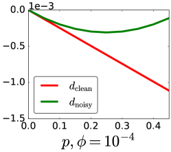
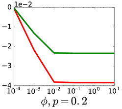
Figure 2: Behavior of Theorem 10 on synthetic data.

(Proof in A.6) Unlike Theorem 8, this bound holds in expectation over the noisy risk RD~,lsubscript𝑅~𝐷𝑙R_{\tilde{D},l}. Its shape depends on the population mean operator, a distribution-dependent quantity. There are two immediate corollaries. When 𝝁𝒟2=0subscriptnormsubscript𝝁𝒟20\|\bm{\mu}_{\mathcal{D}}\|_{2}=0, we obtain optimality for all lols. The second corollary goes further, limiting the minimizers’ distance when losses are differentiable and strongly convex. But even more generally, under proper compactness assumptions on the domain of l𝑙l, Theorem 10 tells us much more: in the case R𝒟~,l(𝜽)subscript𝑅~𝒟𝑙𝜽R_{\tilde{\mathcal{D}},l}(\bm{\theta}) has a unique global minimizer, the smaller 𝝁𝒟2subscriptnormsubscript𝝁𝒟2\|\bm{\mu}_{\mathcal{D}}\|_{2}, the closer the minimizer on noisy data 𝜽~superscript~𝜽\tilde{\bm{\theta}}^{\star} will be to the minimizer on clean data 𝜽superscript𝜽\bm{\theta}^{\star}. Therefore, assuming to know an efficient algorithm that computes a model not far from the global optimum 𝜽~superscript~𝜽\tilde{\bm{\theta}}^{\star}, that will be not far from 𝜽superscript𝜽\bm{\theta}^{\star} either. This is true in spite of the presence of local minima and/or saddle points.

(Long and Servedio, 2010) proves that no convex potential333A convex potential is a loss lC1𝑙superscript𝐶1l\in C^{1}, convex, such that l(0)<0𝑙00l(0)<0 and l(x)0𝑙𝑥0l(x)\rightarrow 0 for x𝑥x\rightarrow\infty. Many convex potentials are lols but not all, but there is no inclusion. An example is exsuperscript𝑒𝑥e^{-x}. is noise tolerant, that is, 00-ALN robust. This is not a contradiction. To show the negative statement, the authors craft a case of 𝒟𝒟\mathcal{D} breaking any of those losses. And in fact that choice of 𝒟𝒟\mathcal{D} does not meet optimality in our bound, because 𝝁𝒟2=14(18γ2+6γ+1)>0subscriptnormsubscript𝝁𝒟21418superscript𝛾26𝛾10\|\bm{\mu}_{\mathcal{D}}\|_{2}=\frac{1}{4}(18\gamma^{2}+6\gamma+1)>0, with γ(0,1/6)𝛾016\gamma\in(0,1/6). In contrast, we show that every element of the broad class of lols is approximately robust, as opposed to a worst-case statement. Finally, compare our ϵitalic-ϵ\epsilon-robustness to the one of (Ghosh et al., 2015): R𝒟,l(𝜽~)(12max(p,p+))1R𝒟,l(𝜽)subscript𝑅𝒟𝑙superscript~𝜽superscript12subscript𝑝subscript𝑝1subscript𝑅𝒟𝑙superscript𝜽R_{\mathcal{D},l}(\tilde{\bm{\theta}}^{*})\leq(1-2\max(p_{-},p_{+}))^{-1}R_{\mathcal{D},l}(\bm{\theta}^{*}). Such bound, while relating the (non-noisy) l𝑙l-risks, is not data-dependent and may be not much informative for high noise rates.

5.2 Experiments

Algorithm 2 𝝁𝝁\bm{\mu}sgd applied on noisy labels
  Input: 𝒮~,llol~𝒮𝑙lol\tilde{\mathcal{S}},l\in\textsc{lol}; λ>0𝜆0\lambda>0; T>0𝑇0T>0
  𝒮2x=.{(𝒙i,σ),i[m],σ𝒴}\mathcal{S}_{2x}\stackrel{{\scriptstyle\mathrm{.}}}{{=}}\{(\bm{x}_{i},\sigma),i\in[m],\forall\sigma\in\mathcal{Y}\}
  𝝁^𝒮~subscript^𝝁~𝒮absent\hat{\bm{\mu}}_{\tilde{\mathcal{S}}}\leftarrow Equation 4
  𝜽𝝁𝜽𝝁\bm{\theta}\leftarrow\bm{\mu}-sgd(𝒮2x,𝝁^𝒮~,λ,T)subscript𝒮2𝑥subscript^𝝁~𝒮𝜆𝑇(\mathcal{S}_{2x},\hat{\bm{\mu}}_{\tilde{\mathcal{S}}},\lambda,T)
  Output: 𝜽𝜽\bm{\theta}

We analyze experimentally the theory so far developed. From now on, we assume to know p+subscript𝑝p_{+} and psubscript𝑝p_{-} at learning time. In principle they can be tuned as hyper-parameters Natarajan et al. (2013), at least for small |𝒴|𝒴|\mathcal{Y}| (Sukhbaatar and Fergus, 2014). While being out of scope, practical noise estimators are studied (Bootkrajang and Kabán, 2012; Liu and Tao, 2014; Menon et al., 2015; Scott, 2015).
Refer to caption
(a) pμ𝒟2𝑝subscriptnormsubscript𝜇𝒟2p\|\mu_{\mathcal{D}}\|_{2} vs. dcleansubscript𝑑cleand_{\mathrm{clean}}
Refer to caption
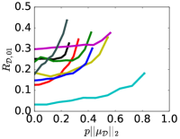
(b) pμ𝒟2𝑝subscriptnormsubscript𝜇𝒟2p\|\mu_{\mathcal{D}}\|_{2} vs. R𝒟,01subscript𝑅𝒟01R_{\mathcal{D},01}
Refer to caption
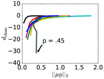
(c) μ𝒟~2subscriptnormsubscript𝜇~𝒟2\|\mu_{\tilde{\mathcal{D}}}\|_{2} vs. dcleansubscript𝑑cleand_{\mathrm{clean}}
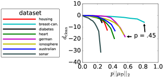
Figure 3: How mean operator and noise rate condition risks. dclean=.R𝒟,l(𝜽)R𝒟,l(𝜽~)superscript.subscript𝑑cleansubscript𝑅𝒟𝑙superscript𝜽subscript𝑅𝒟𝑙superscript~𝜽d_{\mathrm{clean}}\stackrel{{\scriptstyle\mathrm{.}}}{{=}}R_{\mathcal{D},l}(\bm{\theta}^{\star})-R_{\mathcal{D},l}(\tilde{\bm{\theta}}^{\star}).

We begin by building a toy planar dataset to probe the behavior of Theorem 10. It is made of four observations: (0,1)01(0,1) and (ϕ/3,1/3)italic-ϕ313(\phi/3,1/3) three times, with the first example the only negative, repeated 5 times. We consider this the distribution 𝒟𝒟\mathcal{D} so as to calculate 𝝁𝒟2=ϕ2/4subscriptnormsubscript𝝁𝒟2superscriptitalic-ϕ24\|\bm{\mu}_{\mathcal{D}}\|_{2}=\phi^{2}/4. We fix p+,p=0.2=psubscript𝑝subscript𝑝0.2𝑝p_{+},p_{-}=0.2=p and control ϕitalic-ϕ\phi to measure the discrepancy dnoisy=.R𝒟~,l(𝜽)R𝒟~,l(𝜽~)superscript.subscript𝑑noisysubscript𝑅~𝒟𝑙superscript𝜽subscript𝑅~𝒟𝑙superscript~𝜽d_{\mathrm{noisy}}\stackrel{{\scriptstyle\mathrm{.}}}{{=}}R_{\tilde{\mathcal{D}},l}(\bm{\theta}^{\star})-R_{\tilde{\mathcal{D}},l}(\tilde{\bm{\theta}}^{\star}), its counterpart dcleansubscript𝑑cleand_{\mathrm{clean}} computed on 𝒟𝒟\mathcal{D}, and how the two minimizers “differ in sign” by dmodels=.𝜽,𝜽~/𝜽2𝜽~2superscript.subscript𝑑modelssuperscript𝜽superscript~𝜽subscriptnormsuperscript𝜽2subscriptnormsuperscript~𝜽2d_{\mathrm{models}}\stackrel{{\scriptstyle\mathrm{.}}}{{=}}\langle\bm{\theta}^{\star},\tilde{\bm{\theta}}^{\star}\rangle/\|\bm{\theta}^{\star}\|_{2}\|\tilde{\bm{\theta}}^{\star}\|_{2}. The same simulation is run varying the noise rates with constant ϕ=104italic-ϕsuperscript104\phi=10^{-4}. We learn with λ=106𝜆superscript106\lambda=10^{-6} by standard square loss. Results are in Figure 2. The closer the parameters to 00, the smaller dcleandnoisysubscript𝑑cleansubscript𝑑noisyd_{\mathrm{clean}}-d_{\mathrm{noisy}}, while they are equal when each parameter is individually 00. dmodelssubscript𝑑modelsd_{\mathrm{models}} is negligible, which is good news for the 010101-risk on sight.

Algorithm 2 learns with noisy labels on the estimator of Equation 4 and by calling the black box of 𝝁𝝁\bm{\mu}sgd. The next results are based on UCI datasets (Bache and Lichman, 2013). We learn with logistic loss, without model’s intercept and set λ=106𝜆superscript106\lambda=10^{-6} and T=42m𝑇42𝑚T=4\cdot 2m (4 epochs). We measure dcleansubscript𝑑cleand_{\mathrm{clean}} and R𝒟,01subscript𝑅𝒟01R_{\mathcal{D},01}, injecting symmetric label noise p[0,0.45)𝑝00.45p\in[0,0.45) and averaging over 25 runs. Again, we consider the whole distribution so as to play with the ingredients of Theorem 10. Figure 3(a) confirms how the combined effect of p𝝁𝒟2𝑝subscriptnormsubscript𝝁𝒟2p\|\bm{\mu}_{\mathcal{D}}\|_{2} can explain most variation of dcleansubscript𝑑cleand_{\mathrm{clean}}. While this is not strictly implied by Theorem 10 that only involves dnoisysubscript𝑑noisyd_{\mathrm{noisy}}, the observed behavior is expected. A similar picture is given in Figure 3(b) which displays the true risk R𝒟,01subscript𝑅𝒟01R_{\mathcal{D},01} computed on the minimizer 𝜽~superscript~𝜽\tilde{\bm{\theta}}^{\star} of 𝒮~~𝒮\tilde{\mathcal{S}}. From 3(a) and 3(b) we also deduce that large 𝝁𝒟2subscriptnormsubscript𝝁𝒟2\|\bm{\mu}_{\mathcal{D}}\|_{2} is a good proxy for generalization with linear classifiers; see the relative difference between points at the same level of noise. Finally, we have also monitored 𝝁𝒟~subscript𝝁~𝒟\bm{\mu}_{\tilde{\mathcal{D}}}. Figure 3(c) shows that large 𝝁𝒟~2subscriptnormsubscript𝝁~𝒟2\|\bm{\mu}_{\tilde{\mathcal{D}}}\|_{2} indicates small dcleansubscript𝑑cleand_{\mathrm{clean}} as well. This remark can be useful in practice, when the norm can be accurately estimated from 𝒮~~𝒮\tilde{\mathcal{S}}, as opposite to p𝑝p and 𝝁𝒟subscript𝝁𝒟\bm{\mu}_{\mathcal{D}}, and used to anticipate the effect of noise on the task at hand.

We conclude with a systematic study of hold-out error of 𝝁𝝁\bm{\mu}sgd. The same datasets are now split in 1/5 test and 4/5 training sets once at random. In contrast with the previous experimental setting we perform cross-validation of λ10{3,,+3}𝜆superscript1033\lambda\in 10^{\{-3,\dots,+3\}} on 5-folds in the training set. We compare with vanilla sgd run on corrupted sample 𝒮~~𝒮\tilde{\mathcal{S}} and measure the gain from estimating 𝝁^𝒮~subscript^𝝁~𝒮\hat{\bm{\mu}}_{\tilde{\mathcal{S}}}. The other parameters l,T,λ𝑙𝑇𝜆l,T,\lambda are the same for both algorithms; the learning rate η𝜂\eta is untouched from (Shalev-Shwartz et al., 2011) and not tuned for 𝝁𝝁\bm{\mu}sgd. The only differences are in input and gradient update. Table 2 reports test error for sgd and its difference with 𝝁𝝁\bm{\mu}sgd, for a range of values of (p,p+)subscript𝑝subscript𝑝(p_{-},p_{+}). 𝝁𝝁\bm{\mu}sgd beats systematically sgd with large noise rates, and still performs in pair with its competitor under low or null noise. Interestingly, in the presence of very intense noise p+.5subscript𝑝.5p_{+}\approx.5, while the contender is often doomed to random guess, 𝝁𝝁\bm{\mu}sgd still learns sensible models and improves up to 55%percent5555\% relatively to the error of sgd.

(p,p+)subscript𝑝subscript𝑝absent(p_{-},p_{+})\rightarrow (.00,.00).00.00(.00,.00) (.20,.00).20.00(.20,.00) (.20,.10).20.10(.20,.10) (.20,.20).20.20(.20,.20) (.20,.30).20.30(.20,.30) (.20,.40).20.40(.20,.40) (.20,.49).20.49(.20,.49)
dataset sgd 𝝁𝝁\bm{\mu}sgd sgd 𝝁𝝁\bm{\mu}sgd sgd 𝝁𝝁\bm{\mu}sgd sgd 𝝁𝝁\bm{\mu}sgd sgd 𝝁𝝁\bm{\mu}sgd sgd 𝝁𝝁\bm{\mu}sgd sgd 𝝁𝝁\bm{\mu}sgd
australian 0.13 +.01.01+.01 0.15 .01.01\bm{-.01} 0.14 ±.00plus-or-minus.00\pm.00 0.14 +.01.01+.01 0.16 .01.01\bm{-.01} 0.26 .09.09\bm{-.09} 0.45 .25.25\bm{-.25}
breast-can. 0.02 +.01.01+.01 0.03 ±.00plus-or-minus.00\pm.00 0.03 ±.00plus-or-minus.00\pm.00 0.03 ±.00plus-or-minus.00\pm.00 0.05 .01.01\bm{-.01} 0.11 .06.06\bm{-.06} 0.17 .08.08\bm{-.08}
diabetes 0.28 .03.03\bm{-.03} 0.29 .03.03\bm{-.03} 0.29 .03.03\bm{-.03} 0.27 .02.02\bm{-.02} 0.28 .02.02\bm{-.02} 0.39 .13.13\bm{-.13} 0.59 .22.22\bm{-.22}
german 0.27 .02.02\bm{-.02} 0.26 ±.00plus-or-minus.00\pm.00 0.27 .02.02\bm{-.02} 0.29 .02.02\bm{-.02} 0.31 .01.01\bm{-.01} 0.31 ±.00plus-or-minus.00\pm.00 0.31 ±.00plus-or-minus.00\pm.00
heart 0.15 +.01.01+.01 0.17 .01.01\bm{-.01} 0.16 ±.00plus-or-minus.00\pm.00 0.17 ±.00plus-or-minus.00\pm.00 0.18 .01.01\bm{-.01} 0.26 .08.08\bm{-.08} 0.35 .15.15\bm{-.15}
housing 0.17 .03.03\bm{-.03} 0.23 .05.05\bm{-.05} 0.22 .04.04\bm{-.04} 0.20 .02.02\bm{-.02} 0.22 .03.03\bm{-.03} 0.34 .12.12\bm{-.12} 0.41 .13.13\bm{-.13}
ionosphere 0.14 +0505+05 0.19 .05.05\bm{-.05} 0.20 .05.05\bm{-.05} 0.20 .03.03\bm{-.03} 0.21 .03.03\bm{-.03} 0.35 .13.13\bm{-.13} 0.54 .29.29\bm{-.29}
sonar 0.27 ±.00plus-or-minus.00\pm.00 0.29 +.02.02+.02 0.29 +.01.01+.01 0.34 .04.04\bm{-.04} 0.36 .03.03\bm{-.03} 0.43 .10.10\bm{-.10} 0.45 .05.05\bm{-.05}
Table 2: Test error for sgd and 𝝁𝝁\bm{\mu}sgd over 25 trials of artificially corrupted datasets.

6 Discussion and conclusion

Mean and covariance operators  The intuition behind the relevance of the mean operator becomes clear once we rewrite it as follows.

Lemma 11

Let π+=.𝔼𝒮1{y>0}superscript.subscript𝜋subscript𝔼𝒮1𝑦0\pi_{+}\stackrel{{\scriptstyle\mathrm{.}}}{{=}}\mathbb{E}_{\mathcal{S}}1\{y>0\} be the positive label proportion of 𝒮𝒮\mathcal{S}. Then 𝛍𝒮=ov𝒮[𝐱,y]+(2π+1)𝔼𝒮[𝐱].subscript𝛍𝒮subscriptov𝒮𝐱𝑦2subscript𝜋1subscript𝔼𝒮delimited-[]𝐱\bm{\mu}_{\mathcal{S}}=\mathbb{C}\text{ov}_{\mathcal{S}}[\bm{x},y]+(2\pi_{+}-1)\mathbb{E}_{\mathcal{S}}[\bm{x}]\>\>.

(Proof in A.7) We have come to the unsurprising fact that –when observations are centered– the covariance ov𝒮[𝒙,y]subscriptov𝒮𝒙𝑦\mathbb{C}\text{ov}_{\mathcal{S}}[\bm{x},y] is what we need to know about the labels for learning linear models. The rest of the loss may be seen as a data-dependent regularizer. However, notice how the condition 𝝁𝒟2=0subscriptnormsubscript𝝁𝒟20\|\bm{\mu}_{\mathcal{D}}\|_{2}=0 does not implies ov𝒟[𝒙,y]=0subscriptov𝒟𝒙𝑦0\mathbb{C}\text{ov}_{\mathcal{D}}[\bm{x},y]=0, which would make linear classification hard and limit Theorem 10’s validity to degenerate cases. A kernelized version of this Lemma is given in (Song et al., 2009).

The generality of factorization  Factorization is ubiquitous for any (margin) loss, beyond the theory seen so far. A basic fact of real analysis supports it: a function l𝑙l is (uniquely) the sum of an even function lesubscript𝑙𝑒l_{e} and an odd losubscript𝑙𝑜l_{o}:

l(x)=12(l(x)+l(x)+l(x)l(x))=le(x)+lo(x).𝑙𝑥12𝑙𝑥𝑙𝑥𝑙𝑥𝑙𝑥subscript𝑙𝑒𝑥subscript𝑙𝑜𝑥\displaystyle l(x)=\frac{1}{2}\left(l(x)+l(-x)+l(x)-l(-x)\right)=l_{e}(x)+l_{o}(x)\>\>.

One can check that lesubscript𝑙𝑒l_{e} and losubscript𝑙𝑜l_{o} are indeed even and odd (Figure 1). This is actually all we need for the factorization of l𝑙l.

Theorem 12 (Factorization)

For any sample 𝒮𝒮\mathcal{S} and hypothesis hh the empirical l𝑙l-risk can be written as

R𝒮,l(h)=12𝔼𝒮[σ𝒴l(σh(𝒙))]+𝔼𝒮[lo(yh(𝒙))]subscript𝑅𝒮𝑙12subscript𝔼𝒮delimited-[]subscript𝜎𝒴𝑙𝜎𝒙subscript𝔼𝒮delimited-[]subscript𝑙𝑜𝑦𝒙\displaystyle R_{\mathcal{S},l}(h)=\frac{1}{2}\mathbb{E}_{\mathcal{S}}\left[\sum\nolimits_{\sigma\in\mathcal{Y}}l(\sigma h(\bm{x}))\right]+\mathbb{E}_{\mathcal{S}}\Big{[}l_{o}(yh(\bm{x}))\Big{]}

where lo()subscript𝑙𝑜l_{o}(\cdot) is odd and le()=.σ𝒴l(σh())superscript.subscript𝑙𝑒subscript𝜎𝒴𝑙𝜎l_{e}(\cdot)\stackrel{{\scriptstyle\mathrm{.}}}{{=}}\sum_{\sigma\in\mathcal{Y}}l(\sigma h(\cdot)) is even and both uniquely defined.

Its range of validity is exemplified by 010101 loss, a non-convex discontinuous piece-wise linear function, which factors as

le(x)subscript𝑙𝑒𝑥\displaystyle l_{e}(x) ={12x01otherwise,lo(x)absentcases12𝑥01otherwisemissing-subexpressionsubscript𝑙𝑜𝑥\displaystyle=\begin{array}[]{lc}\Big{\{}\begin{array}[]{cc}\frac{1}{2}&x\neq 0\\ 1&\text{otherwise}\end{array},\end{array}l_{o}(x) =12sign(x).absent12sign𝑥\displaystyle=-\frac{1}{2}\operatornamewithlimits{sign}(x)\>\>.

It follows immediately that 𝔼𝒮[lo()]subscript𝔼𝒮delimited-[]subscript𝑙𝑜\mathbb{E}_{\mathcal{S}}[l_{o}(\cdot)] is sufficient for y𝑦y. However, losubscript𝑙𝑜l_{o} is a function of model 𝜽𝜽\bm{\theta}. This defeats the purpose a of sufficient statistic, which we aim to be computable from data only and it is the main reason to define lols. The Factorization Theorem 3 can also be stated for rkhs. To show that, notice that we satisfy all hypotheses of the Representer Theorem (Schölkopf and Smola, 2002).

Theorem 13

Let h(𝐱):𝒳:𝐱𝒳h(\bm{x}):\mathcal{X}\rightarrow\mathcal{H} be a feature map into a Reproducing Kernel Hilbert Space (rkhs) \mathcal{H} with symmetric positive definite kernel k:𝒳×𝒳:𝑘𝒳𝒳k:\mathcal{X}\times\mathcal{X}\rightarrow\mathbb{R}, such that h:𝐱k(,𝐱):𝐱𝑘𝐱h:\bm{x}\rightarrow k(\cdot,\bm{x}). For any learning sample 𝒮𝒮\mathcal{S}, the empirical l𝑙l-risk R𝒮,l(h)subscript𝑅𝒮𝑙R_{\mathcal{S},l}(h) with Ω:h+:Ωsubscriptnormsuperscript\Omega:||h||_{\mathcal{H}}\rightarrow\mathbb{R}^{+} regularization can be written as

12𝔼𝒮[σ𝒴l(σh(𝒙))]+𝔼𝒮[lo(yh(𝒙))]+Ω(h)12subscript𝔼𝒮delimited-[]subscript𝜎𝒴𝑙𝜎𝒙subscript𝔼𝒮delimited-[]subscript𝑙𝑜𝑦𝒙Ωsubscriptnorm\displaystyle\frac{1}{2}\mathbb{E}_{\mathcal{S}}\left[\sum\nolimits_{\sigma\in\mathcal{Y}}l(\sigma h(\bm{x}))\right]+\mathbb{E}_{\mathcal{S}}\Big{[}l_{o}(yh(\bm{x}))\Big{]}+\Omega(||h||_{\mathcal{H}})

and the optimal hypothesis admits a representation of the form h(𝐱)=i[m]αik(𝐱,𝐱i)𝐱subscript𝑖delimited-[]𝑚subscript𝛼𝑖𝑘𝐱subscript𝐱𝑖h(\bm{x})=\sum_{i\in[m]}\alpha_{i}k(\bm{x},\bm{x}_{i}).

All paper may be read in the context of non-parametric models, with the kernel mean operator as sufficient statistic. Finally, it is simple to show factorization for square loss for regression (C). This finding may open further applications of our framework.

The linear-odd losses of (du Plessis et al., 2015)  This recent work in the context of pu shows how the linear-odd condition on a convex l𝑙l allows one to derive a tractable, i.e. still convex, loss for learning with pu. The approach is conceptually related to ours as it isolates a label-free term in the loss, with the goal of leveraging on the unlabelled examples too. Interestingly, the linear term of their Equation 4 can be seen as a mean operator estimator like 𝝁^=.(y=1)𝔼𝒮+[𝒙]superscript.^𝝁𝑦1subscript𝔼subscript𝒮delimited-[]𝒙\hat{\bm{\mu}}\stackrel{{\scriptstyle\mathrm{.}}}{{=}}\mathbb{P}(y=1)\cdot\mathbb{E}_{\mathcal{S}_{+}}[\bm{x}], where 𝒮+subscript𝒮\mathcal{S}_{+} is the set of positive examples. Their manipulation of the loss is not equivalent to the Factorization Theorem 3 though, as explained with details in (D. Beside that, since we reason at the higher level of wsl, we can frame a solution for pu simply calling 𝝁𝝁\bm{\mu}sgd on 𝝁^^𝝁\hat{\bm{\mu}} defined above or on estimators improved by exploiting results of (Patrini et al., 2014).

Learning reductions  Solving a machine learning problem by solutions to other learning problems is a learning reduction (Beygelzimer et al., 2015). Our work does fit into this framework. Following (Beygelzimer et al., 2005), we define a wsl task as a triple (𝒦,𝒴,l)𝒦𝒴𝑙(\mathcal{K},\mathcal{Y},l), with weakly supervised advice 𝒦𝒦\mathcal{K}, predictions space 𝒴𝒴\mathcal{Y} and loss l𝑙l, and we reduce to binary classification (𝒴,𝒴,l)𝒴𝒴𝑙(\mathcal{Y},\mathcal{Y},l). Our reduction is somehow simple, in the sense that 𝒴𝒴\mathcal{Y} does not change and neither does l𝑙l. Although, Algorithm 1 modifies the internal code of the “oracle learner” which contrasts with the concept of reduction. Anyway, we could as well write subgradients as

12(l(𝜽t,𝒙i)+l(𝜽t,𝒙i)+a𝝁),12𝑙superscript𝜽𝑡subscript𝒙𝑖𝑙superscript𝜽𝑡subscript𝒙𝑖𝑎𝝁\displaystyle\frac{1}{2}\left(\partial l(\langle\bm{\theta}^{t},\bm{x}_{i}\rangle)+\partial l(-\langle\bm{\theta}^{t},\bm{x}_{i}\rangle)+a\bm{\mu}\right)\>\>,

which equals l𝑙\partial l, and thus the oracle would be untouched.

Beyond μ𝜇\bm{\mu}sgd  meta-𝝁𝝁\bm{\mu}sgd is intimately similar to stochastic average gradient (sag) (Schmidt et al., 2013). Let denote gei,t(𝜽)le(yi𝜽,𝒙i)superscriptsubscript𝑔𝑒𝑖𝑡𝜽subscript𝑙𝑒subscript𝑦𝑖𝜽subscript𝒙𝑖g_{e}^{i,t}(\bm{\theta})\in\partial l_{e}(y_{i}\langle\bm{\theta},\bm{x}_{i}\rangle) if i=it𝑖superscript𝑖𝑡i=i^{t} (example i𝑖i picked at time t𝑡t), otherwise =gei,t1(𝜽)absentsuperscriptsubscript𝑔𝑒𝑖𝑡1𝜽=g_{e}^{i,t-1}(\bm{\theta}). Define the same for losubscript𝑙𝑜l_{o} accordingly. Then, sag’s model update is:

𝜽t+1𝜽tηmi[m]gei,t(𝜽t)ηmi[m]goi,t(𝜽t),superscript𝜽𝑡1superscript𝜽𝑡𝜂𝑚subscript𝑖delimited-[]𝑚superscriptsubscript𝑔𝑒𝑖𝑡superscript𝜽𝑡𝜂𝑚subscript𝑖delimited-[]𝑚superscriptsubscript𝑔𝑜𝑖𝑡superscript𝜽𝑡\displaystyle\bm{\theta}^{t+1}\leftarrow\bm{\theta}^{t}-\frac{\eta}{m}\sum\nolimits_{i\in[m]}g_{e}^{i,t}(\bm{\theta}^{t})-\frac{\eta}{m}\sum\nolimits_{i\in[m]}g_{o}^{i,t}(\bm{\theta}^{t})\>\>,

and recalling that a𝝁𝒮=𝔼𝒮[lo(𝜽)]𝑎subscript𝝁𝒮subscript𝔼𝒮delimited-[]subscript𝑙𝑜𝜽a\bm{\mu}_{\mathcal{S}}=\mathbb{E}_{\mathcal{S}}[\partial l_{o}(\bm{\theta})], 𝝁𝝁\bm{\mu}sgd’s update is

𝜽t+1𝜽tηlei(𝜽t)ηmi[m]loi(𝜽t).superscript𝜽𝑡1superscript𝜽𝑡𝜂superscriptsubscript𝑙𝑒𝑖superscript𝜽𝑡𝜂𝑚subscript𝑖delimited-[]𝑚superscriptsubscript𝑙𝑜𝑖superscript𝜽𝑡\displaystyle\bm{\theta}^{t+1}\leftarrow\bm{\theta}^{t}-\eta~{}\partial l_{e}^{i}(\bm{\theta}^{t})-\frac{\eta}{m}\sum\nolimits_{i\in[m]}\partial l_{o}^{i}(\bm{\theta}^{t})\>\>.

From this parallel, the two algorithms appear to be variants of a more general sampling mechanism of examples and gradient components, at each step. More generally, stochastic gradient is just one suit of algorithms that fits into our 2-step learning framework. Proximal methods (Bach et al., 2012) are another noticeable example. The same modus operandi leads to a proximal step of the form:

𝜽t+1proxΘ(𝜽t+η(R𝒮2x,l(𝜽t)+a2𝝁))superscript𝜽𝑡1subscriptproxΘsuperscript𝜽𝑡𝜂subscript𝑅subscript𝒮2𝑥𝑙superscript𝜽𝑡𝑎2𝝁\displaystyle\bm{\theta}^{t+1}\leftarrow\mathrm{prox}_{\Theta}\left(\bm{\theta}^{t}+\eta\left(\partial R_{\mathcal{S}_{2x},l}(\bm{\theta}^{t})+\frac{a}{2}\bm{\mu}\right)\right)

with proxg(x)=argminxg(x)+12xx22)\mathrm{prox}_{g}(x)=\operatornamewithlimits{argmin}_{x^{\prime}}g(x^{\prime})+\frac{1}{2}\|x-x^{\prime}\|_{2}^{2}) and Θ()Θ\Theta(\cdot) the regularizer. Once again, the adaptation works by summing 𝝁𝝁\bm{\mu} in the gradient step and changing the input to 𝒮2xsubscript𝒮2𝑥\mathcal{S}_{2x}.

A better (?) picture of robustness  The data-dependent worst-case result of (Long and Servedio, 2010), like any extreme-case argument, should be handled with care. It does not give the big picture for all data we may encounter in a real world, but only the most pessimistic. We present such a global view which appears better than expected: learning the minimizer from noisy data does not necessarily reduce convex losses to a singleton (van Rooyen et al., 2015) but depends on the mean operator for a large number of them (not necessarily linear, convex or smooth). Quite surprisingly, factorization also marries the two opposite views in one formula444See (Ghosh et al., 2015, Theorem 1).:

l(x)=12(l(x)+l(x)=const0-aln+l(x)l(x)=axϵ-aln).𝑙𝑥12subscript𝑙𝑥𝑙𝑥absentconstabsent0-alnsubscript𝑙𝑥𝑙𝑥absent𝑎𝑥absentitalic-ϵ-aln\displaystyle l(x)=\frac{1}{2}(~{}\underbrace{l(x)+l(-x)}_{=\mathrm{const}~{}\Rightarrow~{}0\text{-{aln}}}+\underbrace{l(x)-l(-x)}_{=ax~{}\Rightarrow~{}\epsilon\text{-{aln}}}~{})\>\>.

To conclude, we have seen how losses factor in a way that we can isolate the contribution of supervision. This has several implications both on theoretical and practical grounds: learning theory, formal analysis of label noise robustness, and adaptation of algorithms to handle poorly labelled data. An interesting question is whether factorization would let one identify what really matters in learning that is instead completely unsupervised, and to do so with more complex models than the ones considered here, as for example deep architectures.

Acknowledgements

The authors thank Aditya Menon for insightful feedback on an earlier draft. NICTA is funded by the Australian Government through the Department of Communications and the Australian Research Council through the ICT Center of Excellence Program.

References

  • Lehmann and Casella (1998) E. L. Lehmann and G. Casella. Theory of point estimation, volume 31. Springer Science & Business Media, 1998.
  • Kakade et al. (2009) S. M. Kakade, K. Sridharan, and A. Tewari. On the complexity of linear prediction: Risk bounds, margin bounds, and regularization. In NIPS*23, 2009.
  • du Plessis et al. (2015) M C. du Plessis, G. Niu, and M. Sugiyama. Convex formulation for learning from positive and unlabeled data. In 32th𝑡{}^{~{}th} ICML, pages 1386–1394, 2015.
  • Garcıa-Garcıa and Williamson (2011) D. Garcıa-Garcıa and R. C. Williamson. Degrees of supervision. In NIPS*25 workshop on Relations between machine learning problems, 2011.
  • Hernandez-Gonzalez et al. (2016) J. Hernandez-Gonzalez, I. Inza, and J.A. Lozano. Weak supervision and other non-standard classification problems: a taxonomy. In Pattern Recognition Letters, pages 49–55. Elsevier, 2016.
  • Natarajan et al. (2013) N. Natarajan, I. S. Dhillon, P. K. Ravikumar, and A. Tewari. Learning with noisy labels. In NIPS*27, 2013.
  • Chapelle et al. (2006) O. Chapelle, B. Schölkopf, and A. Zien. Semi-supervised learning. MIT press Cambridge, 2006.
  • Dietterich et al. (1997) T. G. Dietterich, R. H. Lathrop, and T. Lozano-Pérez. Solving the multiple instance problem with axis-parallel rectangles. Artificial Intelligence, 89:31–71, 1997.
  • Quadrianto et al. (2009) N. Quadrianto, A. J. Smola, T. S. Caetano, and Q. V. Le. Estimating labels from label proportions. JMLR, 10:2349–2374, 2009.
  • Joulin and Bach (2012) A. Joulin and F. R. Bach. A convex relaxation for weakly supervised classifiers. In 29th𝑡{}^{~{}th} ICML, 2012.
  • Patrini et al. (2014) G. Patrini, R. Nock, P. Rivera, and T. Caetano. (Almost) no label no cry. In NIPS*28, 2014.
  • van Rooyen et al. (2015) B. van Rooyen, A. K. Menon, and R. C. Williamson. Learning with symmetric label noise: The importance of being unhinged. In NIPS*29, 2015.
  • Gao et al. (2016) W. Gao, L. Wang, Y.-F. Li, and Z.-H Zhou. Risk minimization in the presence of label noise. In Proc. of the 30th AAAI Conference on Artificial Intelligence, 2016.
  • Long and Servedio (2010) P. M. Long and R. A. Servedio. Random classification noise defeats all convex potential boosters. Machine learning, 78(3):287–304, 2010.
  • Stempfel and Ralaivola (2009) G. Stempfel and L. Ralaivola. Learning SVMs from sloppily labeled data. In Artificial Neural Networks (ICANN), pages 884–893. Springer, 2009.
  • Masnadi-Shirazi et al. (2010) H. Masnadi-Shirazi, V. Mahadevan, and N. Vasconcelos. On the design of robust classifiers for computer vision. In Proc. of the 23rd IEEE CVPR, pages 779–786. IEEE, 2010.
  • Ding and Vishwanathan (2010) N. Ding and S. V. N. Vishwanathan. t-logistic regression. In NIPS*24, pages 514–522, 2010.
  • Patrini et al. (2015) G. Patrini, F. Nielsen, and R. Nock. Bridging weak supervision and privacy aware learning via sufficient statistics. NIPS*29, Workshop on learning and privacy with incomplete data and weak supervision, 2015.
  • Chaudhuri and Hsu (2011) K. Chaudhuri and D. Hsu. Sample complexity bounds for differentially private learning. In JMLR, volume 2011, page 155, 2011.
  • Reid and Williamson (2010) M. D. Reid and R. C. Williamson. Composite binary losses. JMLR, 11:2387–2422, 2010.
  • Smola et al. (2007) A. Smola, A. Gretton, L. Song, and B. Schölkopf. A Hilbert space embedding for distributions. In Algorithmic Learning Theory, pages 13–31. Springer, 2007.
  • Nock and Nielsen (2009) R. Nock and F. Nielsen. Bregman divergences and surrogates for learning. IEEE Trans.PAMI, 31:2048–2059, 2009.
  • Jaakkola and Jordan (2000) T. S. Jaakkola and M. I. Jordan. Bayesian parameter estimation via variational methods. Statistics and Computing, 10(1):25–37, 2000.
  • Kearns and Mansour (1996) M. J. Kearns and Y. Mansour. On the boosting ability of top-down decision tree learning algorithms. In 28th𝑡{}^{~{}th} ACM STOC, pages 459–468, 1996.
  • Masnadi-Shirazi (2011) H. Masnadi-Shirazi. The design of bayes consistent loss functions for classification. PhD thesis, University of California at San Diego, 2011.
  • Bartlett and Mendelson (2002) P.-L. Bartlett and S. Mendelson. Rademacher and gaussian complexities: Risk bounds and structural results. JMLR, 3:463–482, 2002.
  • Altun and Smola (2006) Y. Altun and A. J. Smola. Unifying divergence minimization and statistical inference via convex duality. In 19th𝑡{}^{~{}th} COLT, 2006.
  • Shalev-Shwartz et al. (2011) S. Shalev-Shwartz, Y. Singer, N. Srebro, and A. Cotter. Pegasos: Primal estimated sub-gradient solver for svm. Mathematical programming, 127(1):3–30, 2011.
  • Ghosh et al. (2015) A. Ghosh, N. Manwani, and P. S. Sastry. Making risk minimization tolerant to label noise. Neurocomputing, 160:93–107, 2015.
  • Sukhbaatar and Fergus (2014) S. Sukhbaatar and R. Fergus. Learning from noisy labels with deep neural networks. arXiv:1406.2080, 2014.
  • Bootkrajang and Kabán (2012) J. Bootkrajang and A. Kabán. Label-noise robust logistic regression and its applications. In Machine Learning and Knowledge Discovery in Databases, pages 143–158. Springer, 2012.
  • Liu and Tao (2014) T. Liu and D. Tao. Classification with noisy labels by importance reweighting. arXiv:1411.7718, 2014.
  • Menon et al. (2015) A. Menon, B. Van Rooyen, C. S. Ong, and B. Williamson. Learning from corrupted binary labels via class-probability estimation. In 32th𝑡{}^{~{}th} ICML, 2015.
  • Scott (2015) C. Scott. A rate of convergence for mixture proportion estimation, with application to learning from noisy labels. In 18th AISTATS, 2015.
  • Bache and Lichman (2013) K. Bache and M. Lichman. UCI machine learning repository, 2013. URL http://archive.ics.uci.edu/ml.
  • Song et al. (2009) L. Song, J. Huang, A. J. Smola, and K. Fukumizu. Hilbert space embeddings of conditional distributions with applications to dynamical systems. In 26th𝑡{}^{~{}th} ICML. ACM, 2009.
  • Schölkopf and Smola (2002) B. Schölkopf and A. J. Smola. Learning with kernels: Support vector machines, regularization, optimization, and beyond. MIT press, 2002.
  • Beygelzimer et al. (2015) A. Beygelzimer, H. Daumé III, J. Langford, and P. Mineiro. Learning reductions that really work. arXiv:1502.02704, 2015.
  • Beygelzimer et al. (2005) A. Beygelzimer, V. Dani, T. Hayes, J. Langford, and B. Zadrozny. Error limiting reductions between classification tasks. In 22th𝑡{}^{~{}th} ICML, pages 49–56, 2005.
  • Schmidt et al. (2013) M. Schmidt, N. L. Roux, and F. Bach. Minimizing finite sums with the stochastic average gradient. arXiv:1309.2388, 2013.
  • Bach et al. (2012) F. Bach, R. Jenatton, J. Mairal, and G. Obozinski. Optimization with sparsity-inducing penalties. Foundations and Trends® in Machine Learning, 4(1):1–106, 2012.
  • McDiarmid (1998) C. McDiarmid. Concentration. In M. Habib, C. McDiarmid, J. Ramirez-Alfonsin, and B. Reed, editors, Probabilistic Methods for Algorithmic Discrete Mathematics, pages 1–54. Springer Verlag, 1998.
  • Manwani and Sastry (2013) N. Manwani and P. S. Sastry. Noise tolerance under risk minimization. Cybernetics, IEEE Transactions on, 43(3):1146–1151, 2013.

Appendices

Appendix A Proofs

A.1 Proof of Lemma 5

We need to show the double implication that defines sufficiency for y𝑦y.
)\Rightarrow) By Factorization Theorem (3), R𝒮,l(h)R𝒮,l(h)subscript𝑅𝒮𝑙subscript𝑅superscript𝒮𝑙R_{\mathcal{S},l}(h)-R_{\mathcal{S}^{\prime},l}(h) is label independent only if the odd part cancels out.
)\Leftarrow) If 𝝁𝒮=𝝁𝒮subscript𝝁𝒮superscriptsubscript𝝁𝒮\bm{\mu}_{\mathcal{S}}=\bm{\mu}_{\mathcal{S}}^{\prime} then R𝒮,l(h)R𝒮,l(h)subscript𝑅𝒮𝑙subscript𝑅superscript𝒮𝑙R_{\mathcal{S},l}(h)-R_{\mathcal{S}^{\prime},l}(h) is independent of the label, because the label only appears in the mean operator due to Factorization Theorem (3).

A.2 Proof of Lemma 6

Consider the class of lols satisfying l(x)l(x)=2ax𝑙𝑥𝑙𝑥2𝑎𝑥l(x)-l(-x)=2ax. For any element of the class, define le(x)=l(x)axsubscript𝑙𝑒𝑥𝑙𝑥𝑎𝑥l_{e}(x)=l(x)-ax, which is even. In fact we have

le(x)=l(x)+ax=l(x)2ax+ax=l(x)ax=le(x).subscript𝑙𝑒𝑥𝑙𝑥𝑎𝑥𝑙𝑥2𝑎𝑥𝑎𝑥𝑙𝑥𝑎𝑥subscript𝑙𝑒𝑥l_{e}(-x)=l(-x)+ax=l(x)-2ax+ax=l(x)-ax=l_{e}(x)\>\>.

A.3 Proof of Theorem 7

We start by proving two helper Lemmas. The next one provides a bound to the Rademacher complexity computed on the sample 𝒮2x=.{(𝒙i,σ),i[m],σ𝒴}\mathcal{S}_{2x}\stackrel{{\scriptstyle\mathrm{.}}}{{=}}\{(\bm{x}_{i},\sigma),i\in[m],\forall\sigma\in\mathcal{Y}\}.

Lemma 14

Suppose m𝑚m even. Suppose 𝒳={𝐱:𝐱2X}𝒳conditional-set𝐱subscriptnorm𝐱2𝑋\mathcal{X}=\{\bm{x}:\|\bm{x}\|_{2}\leq X\} be the observations space, and ={𝛉:𝛉2B}conditional-set𝛉subscriptnorm𝛉2𝐵\mathcal{H}=\{\bm{\theta}:\|\bm{\theta}\|_{2}\leq B\} be the space of linear hypotheses. Let 𝒴2m=.×j[2m]𝒴\mathcal{Y}^{2m}\stackrel{{\scriptstyle\mathrm{.}}}{{=}}\times_{j\in[2m]}\mathcal{Y}. Then the empirical Rademacher complexity

(𝒮2x)=.𝔼σ𝒴2m[sup𝜽12mi[2m]σi𝜽,𝒙i]superscript.subscript𝒮2𝑥subscript𝔼similar-to𝜎superscript𝒴2𝑚delimited-[]subscriptsupremum𝜽12𝑚subscript𝑖delimited-[]2𝑚subscript𝜎𝑖𝜽subscript𝒙𝑖\mathcal{R}(\mathcal{H}\circ\mathcal{S}_{2x})\stackrel{{\scriptstyle\mathrm{.}}}{{=}}\mathbb{E}_{\sigma\sim\mathcal{Y}^{2m}}\left[\sup_{\bm{\theta}\in\mathcal{H}}\frac{1}{2m}\sum_{i\in[2m]}\sigma_{i}\langle\bm{\theta},\bm{x}_{i}\rangle\right]

of \mathcal{H} on 𝒮2xsubscript𝒮2𝑥\mathcal{S}_{2x} satisfies:

(𝒮2x)subscript𝒮2𝑥\displaystyle\mathcal{R}(\mathcal{H}\circ\mathcal{S}_{2x}) \displaystyle\leq vBX2m,𝑣𝐵𝑋2𝑚\displaystyle v\cdot\frac{BX}{\sqrt{2m}}\>\>, (5)

with v=.12+12121msuperscript.𝑣1212121𝑚v\stackrel{{\scriptstyle\mathrm{.}}}{{=}}\frac{1}{2}+\frac{1}{2}\sqrt{\frac{1}{2}-\frac{1}{m}}.

Proof.

Suppose without loss of generality that 𝒙i=𝒙m+isubscript𝒙𝑖subscript𝒙𝑚𝑖\bm{x}_{i}=\bm{x}_{m+i}. The proof relies on the observation that 𝝈𝒴2mfor-all𝝈superscript𝒴2𝑚\forall\bm{\sigma}\in\mathcal{Y}^{2m},

argsup𝜽{𝔼𝒮[σ(𝒙)𝜽,𝒙]}subscriptsupremum𝜽subscript𝔼𝒮delimited-[]𝜎𝒙𝜽𝒙\displaystyle\arg\sup_{\bm{\theta}\in{\mathcal{H}}}\left\{\mathbb{E}_{{\mathcal{S}}}[\sigma(\bm{x})\langle\bm{\theta},\bm{x}\rangle]\right\} =\displaystyle= 12margsup𝜽{iσi𝜽,𝒙i}12𝑚subscriptsupremum𝜽subscript𝑖subscript𝜎𝑖𝜽subscript𝒙𝑖\displaystyle\frac{1}{2m}\arg\sup_{\bm{\theta}\in{\mathcal{H}}}\left\{\sum_{i}{\sigma_{i}\langle\bm{\theta},\bm{x}_{i}\rangle}\right\} (6)
=\displaystyle= sup𝜽2iσi𝒙i2iσi𝒙i.subscriptsupremumsubscriptnorm𝜽2subscriptnormsubscript𝑖subscript𝜎𝑖subscript𝒙𝑖2subscript𝑖subscript𝜎𝑖subscript𝒙𝑖\displaystyle\frac{\sup_{{\mathcal{H}}}\|\bm{\theta}\|_{2}}{\|\sum_{i}{\sigma_{i}\bm{x}_{i}}\|_{2}}\sum_{i}{\sigma_{i}\bm{x}_{i}}\>\>.

So,

(𝒮2x)subscript𝒮2𝑥\displaystyle\mathcal{R}(\mathcal{H}\circ\mathcal{S}_{2x}) =\displaystyle= 𝔼𝒴2msuph{𝔼𝒮2x[σ(𝒙)h(𝒙)]}subscript𝔼superscript𝒴2𝑚subscriptsupremumsubscript𝔼subscript𝒮2𝑥delimited-[]𝜎𝒙𝒙\displaystyle\mathbb{E}_{\mathcal{Y}^{2m}}\sup_{h\in{\mathcal{H}}}\left\{\mathbb{E}_{{\mathcal{S}}_{2x}}[\sigma(\bm{x})h(\bm{x})]\right\} (7)
=\displaystyle= supθ22m𝔼𝒴2m[(i=12mσi𝒙i)(i=12mσi𝒙i)i=12mσi𝒙i2]subscriptsupremumsubscriptnorm𝜃22𝑚subscript𝔼superscript𝒴2𝑚delimited-[]superscriptsuperscriptsubscript𝑖12𝑚subscript𝜎𝑖subscript𝒙𝑖topsuperscriptsubscript𝑖12𝑚subscript𝜎𝑖subscript𝒙𝑖subscriptnormsuperscriptsubscript𝑖12𝑚subscript𝜎𝑖subscript𝒙𝑖2\displaystyle\frac{\sup_{{\mathcal{H}}}\|\theta\|_{2}}{2m}\cdot\mathbb{E}_{\mathcal{Y}^{2m}}\left[\frac{\left(\sum_{i=1}^{2m}{\sigma_{i}\bm{x}_{i}}\right)^{\top}\left(\sum_{i=1}^{2m}{\sigma_{i}\bm{x}_{i}}\right)}{\|\sum_{i=1}^{2m}{\sigma_{i}\bm{x}_{i}}\|_{2}}\right]
=\displaystyle= supθ2𝔼𝒴2m[12mi=12mσi𝒙i2].subscriptsupremumsubscriptnorm𝜃2subscript𝔼superscript𝒴2𝑚delimited-[]12𝑚subscriptnormsuperscriptsubscript𝑖12𝑚subscript𝜎𝑖subscript𝒙𝑖2\displaystyle\sup_{{\mathcal{H}}}\|\theta\|_{2}\cdot\mathbb{E}_{\mathcal{Y}^{2m}}\left[\frac{1}{2m}\cdot\left\|\sum_{i=1}^{2m}{\sigma_{i}\bm{x}_{i}}\right\|_{2}\right]\>\>.

Now, remark that whenever σi=σm+isubscript𝜎𝑖subscript𝜎𝑚𝑖\sigma_{i}=-\sigma_{m+i}, 𝒙isubscript𝒙𝑖\bm{x}_{i} disappears in the sum, and therefore the max norm for the sum may decrease as well. This suggests to split the 22msuperscript22𝑚2^{2m} assignations into 2msuperscript2𝑚2^{m} groups of size 2msuperscript2𝑚2^{m}, ranging over the possible number of observations taken into account in the sum. They can be factored by a weighted sum of contributions of each subset of indices [m]delimited-[]𝑚{\mathcal{I}}\subseteq[m] ranging over the non-duplicated observations:

𝔼𝒴2m[1mi=12mσi𝒙i2]subscript𝔼superscript𝒴2𝑚delimited-[]1𝑚subscriptnormsuperscriptsubscript𝑖12𝑚subscript𝜎𝑖subscript𝒙𝑖2\displaystyle\mathbb{E}_{\mathcal{Y}^{2m}}\left[\frac{1}{m}\cdot\left\|\sum_{i=1}^{2m}{\sigma_{i}\bm{x}_{i}}\right\|_{2}\right] =\displaystyle= 122m[m]2m||2m𝝈𝒴||2iσi𝒙i2.1superscript22𝑚subscriptdelimited-[]𝑚superscript2𝑚2𝑚subscript𝝈superscript𝒴2subscriptnormsubscript𝑖subscript𝜎𝑖subscript𝒙𝑖2\displaystyle\frac{1}{2^{2m}}\sum_{{\mathcal{I}}\subseteq[m]}\frac{2^{m-|{\mathcal{I}}|}}{2m}\cdot\sum_{\bm{\sigma}\in\mathcal{Y}^{|{\mathcal{I}}|}}\sqrt{2}\left\|\sum_{i\in{\mathcal{I}}}{\sigma_{i}\bm{x}_{i}}\right\|_{2}\>\>. (8)
=\displaystyle= 22m[m]12m12||𝝈𝒴||iσi𝒙i2u||.2superscript2𝑚subscriptdelimited-[]𝑚12𝑚subscript1superscript2subscript𝝈superscript𝒴subscriptnormsubscript𝑖subscript𝜎𝑖subscript𝒙𝑖2subscript𝑢\displaystyle\frac{\sqrt{2}}{2^{m}}\sum_{{\mathcal{I}}\subseteq[m]}\frac{1}{2m}\cdot\underbrace{\frac{1}{2^{|{\mathcal{I}}|}}\cdot\sum_{\bm{\sigma}\in\mathcal{Y}^{|{\mathcal{I}}|}}\left\|\sum_{i\in{\mathcal{I}}}{\sigma_{i}\bm{x}_{i}}\right\|_{2}}_{u_{|{\mathcal{I}}|}}\>\>. (9)

The 22\sqrt{2} factor appears because of the fact that we now consider only the observations of 𝒮𝒮{\mathcal{S}}. Now, for any fixed {\mathcal{I}}, we renumber its observations in [||]delimited-[][|{\mathcal{I}}|] for simplicity, and observe that, since 1+x1+x/21𝑥1𝑥2\sqrt{1+x}\leq 1+x/2,

u||subscript𝑢\displaystyle u_{|{\mathcal{I}}|} =\displaystyle= 12||𝝈𝒴||i𝒙i22+i1i2σi1σi2𝒙i1𝒙i21superscript2subscript𝝈superscript𝒴subscript𝑖superscriptsubscriptnormsubscript𝒙𝑖22subscriptsubscript𝑖1subscript𝑖2subscript𝜎subscript𝑖1subscript𝜎subscript𝑖2superscriptsubscript𝒙subscript𝑖1topsubscript𝒙subscript𝑖2\displaystyle\frac{1}{2^{|{\mathcal{I}}|}}\sum_{\bm{\sigma}\in\mathcal{Y}^{|{\mathcal{I}}|}}{\sqrt{\sum_{i\in{\mathcal{I}}}\|\bm{x}_{i}\|_{2}^{2}+\sum_{i_{1}\neq i_{2}}{\sigma_{i_{1}}\sigma_{i_{2}}\bm{x}_{i_{1}}^{\top}\bm{x}_{i_{2}}}}} (10)
=\displaystyle= i𝒙i222||𝝈𝒴||1+i1i2σi1σi2𝒙i1𝒙i2i𝒙i22subscript𝑖superscriptsubscriptnormsubscript𝒙𝑖22superscript2subscript𝝈superscript𝒴1subscriptsubscript𝑖1subscript𝑖2subscript𝜎subscript𝑖1subscript𝜎subscript𝑖2superscriptsubscript𝒙subscript𝑖1topsubscript𝒙subscript𝑖2subscript𝑖superscriptsubscriptnormsubscript𝒙𝑖22\displaystyle\frac{\sqrt{\sum_{i\in{\mathcal{I}}}\|\bm{x}_{i}\|_{2}^{2}}}{2^{|{\mathcal{I}}|}}\sum_{\bm{\sigma}\in\mathcal{Y}^{|{\mathcal{I}}|}}\sqrt{1+\frac{\sum_{i_{1}\neq i_{2}}{\sigma_{i_{1}}\sigma_{i_{2}}\bm{x}_{i_{1}}^{\top}\bm{x}_{i_{2}}}}{\sum_{i\in{\mathcal{I}}}\|\bm{x}_{i}\|_{2}^{2}}} (11)
\displaystyle\leq i𝒙i222||𝝈𝒴||(1+i1i2σi1σi2𝒙i1𝒙i22i𝒙i22)subscript𝑖superscriptsubscriptnormsubscript𝒙𝑖22superscript2subscript𝝈superscript𝒴1subscriptsubscript𝑖1subscript𝑖2subscript𝜎subscript𝑖1subscript𝜎subscript𝑖2superscriptsubscript𝒙subscript𝑖1topsubscript𝒙subscript𝑖22subscript𝑖superscriptsubscriptnormsubscript𝒙𝑖22\displaystyle\frac{\sqrt{\sum_{i\in{\mathcal{I}}}\|\bm{x}_{i}\|_{2}^{2}}}{2^{|{\mathcal{I}}|}}\sum_{\bm{\sigma}\in\mathcal{Y}^{|{\mathcal{I}}|}}\left(1+\frac{\sum_{i_{1}\neq i_{2}}{\sigma_{i_{1}}\sigma_{i_{2}}\bm{x}_{i_{1}}^{\top}\bm{x}_{i_{2}}}}{2\sum_{i\in{\mathcal{I}}}\|\bm{x}_{i}\|_{2}^{2}}\right) (12)
=\displaystyle= i𝒙i22+12||2i𝒙i22𝝈𝒴||i1i2σi1σi2𝒙i1𝒙i2subscript𝑖superscriptsubscriptnormsubscript𝒙𝑖221superscript22subscript𝑖superscriptsubscriptnormsubscript𝒙𝑖22subscript𝝈superscript𝒴subscriptsubscript𝑖1subscript𝑖2subscript𝜎subscript𝑖1subscript𝜎subscript𝑖2superscriptsubscript𝒙subscript𝑖1topsubscript𝒙subscript𝑖2\displaystyle\sqrt{\sum_{i\in{\mathcal{I}}}\|\bm{x}_{i}\|_{2}^{2}}+\frac{1}{2^{|{\mathcal{I}}|}\cdot 2\sum_{i\in{\mathcal{I}}}\|\bm{x}_{i}\|_{2}^{2}}\cdot\sum_{\bm{\sigma}\in\mathcal{Y}^{|{\mathcal{I}}|}}\sum_{i_{1}\neq i_{2}}{\sigma_{i_{1}}\sigma_{i_{2}}\bm{x}_{i_{1}}^{\top}\bm{x}_{i_{2}}} (13)
=\displaystyle= i𝒙i22+12||2i𝒙i22i1i2𝒙i1𝒙i2(𝝈𝒴||σi1σi2)=0subscript𝑖superscriptsubscriptnormsubscript𝒙𝑖221superscript22subscript𝑖superscriptsubscriptnormsubscript𝒙𝑖22subscriptsubscript𝑖1subscript𝑖2superscriptsubscript𝒙subscript𝑖1topsubscript𝒙subscript𝑖2subscriptsubscript𝝈superscript𝒴subscript𝜎subscript𝑖1subscript𝜎subscript𝑖2absent0\displaystyle\sqrt{\sum_{i\in{\mathcal{I}}}\|\bm{x}_{i}\|_{2}^{2}}+\frac{1}{2^{|{\mathcal{I}}|}\cdot 2\sum_{i\in{\mathcal{I}}}\|\bm{x}_{i}\|_{2}^{2}}\cdot\sum_{i_{1}\neq i_{2}}{\bm{x}_{i_{1}}^{\top}\bm{x}_{i_{2}}\cdot\underbrace{\left(\sum_{\bm{\sigma}\in\mathcal{Y}^{|{\mathcal{I}}|}}\sigma_{i_{1}}\sigma_{i_{2}}\right)}_{=0}} (14)
=\displaystyle= i𝒙i22subscript𝑖superscriptsubscriptnormsubscript𝒙𝑖22\displaystyle\sqrt{\sum_{i\in{\mathcal{I}}}\|\bm{x}_{i}\|_{2}^{2}} (15)
\displaystyle\leq ||X.𝑋\displaystyle\sqrt{|\mathcal{I}|}\cdot X\>\>. (16)

Plugging this in eq. (9) yields

1X𝔼𝒴2m[1mi=12mσi𝒙i2]1𝑋subscript𝔼superscript𝒴2𝑚delimited-[]1𝑚subscriptnormsuperscriptsubscript𝑖12𝑚subscript𝜎𝑖subscript𝒙𝑖2\displaystyle\frac{1}{X}\cdot\mathbb{E}_{\mathcal{Y}^{2m}}\left[\frac{1}{m}\cdot\left\|\sum_{i=1}^{2m}{\sigma_{i}\bm{x}_{i}}\right\|_{2}\right] \displaystyle\leq 22mk=0mk2m(mk).2superscript2𝑚superscriptsubscript𝑘0𝑚𝑘2𝑚binomial𝑚𝑘\displaystyle\frac{\sqrt{2}}{2^{m}}\sum_{k=0}^{m}\frac{\sqrt{k}}{2m}{m\choose k}\>\>. (17)

Since m𝑚m is even:

𝔼𝒴2m[12mi=12mσi𝒙i2]subscript𝔼superscript𝒴2𝑚delimited-[]12𝑚subscriptnormsuperscriptsubscript𝑖12𝑚subscript𝜎𝑖subscript𝒙𝑖2\displaystyle\mathbb{E}_{\mathcal{Y}^{2m}}\left[\frac{1}{2m}\cdot\left\|\sum_{i=1}^{2m}{\sigma_{i}\bm{x}_{i}}\right\|_{2}\right] \displaystyle\leq 22mk=0(m/2)1k2m(mk)+22mk=m/2mk2m(mk).2superscript2𝑚superscriptsubscript𝑘0𝑚21𝑘2𝑚binomial𝑚𝑘2superscript2𝑚superscriptsubscript𝑘𝑚2𝑚𝑘2𝑚binomial𝑚𝑘\displaystyle\frac{\sqrt{2}}{2^{m}}\sum_{k=0}^{(m/2)-1}\frac{\sqrt{k}}{2m}{m\choose k}+\frac{\sqrt{2}}{2^{m}}\sum_{k=m/2}^{m}\frac{\sqrt{k}}{2m}{m\choose k}\>\>. (18)

Notice that the left one trivially satisfies

22mk=0(m/2)1k2m(mk)2superscript2𝑚superscriptsubscript𝑘0𝑚21𝑘2𝑚binomial𝑚𝑘\displaystyle\frac{\sqrt{2}}{2^{m}}\sum_{k=0}^{(m/2)-1}\frac{\sqrt{k}}{2m}{m\choose k} \displaystyle\leq 22mk=0(m/2)112mm22(mk)2superscript2𝑚superscriptsubscript𝑘0𝑚2112𝑚𝑚22binomial𝑚𝑘\displaystyle\frac{\sqrt{2}}{2^{m}}\sum_{k=0}^{(m/2)-1}\frac{1}{2m}\cdot\sqrt{\frac{m-2}{2}}{m\choose k} (19)
=\displaystyle= 121m2m212mk=0(m/2)1(mk)121𝑚2superscript𝑚21superscript2𝑚superscriptsubscript𝑘0𝑚21binomial𝑚𝑘\displaystyle\frac{1}{2}\cdot\sqrt{\frac{1}{m}-\frac{2}{m^{2}}}\cdot\frac{1}{2^{m}}\sum_{k=0}^{(m/2)-1}{m\choose k}
\displaystyle\leq 141m2m2141𝑚2superscript𝑚2\displaystyle\frac{1}{4}\cdot\sqrt{\frac{1}{m}-\frac{2}{m^{2}}}

Also, the right one satisfies:

22mk=m/2mk2m(mk)2superscript2𝑚superscriptsubscript𝑘𝑚2𝑚𝑘2𝑚binomial𝑚𝑘\displaystyle\frac{\sqrt{2}}{2^{m}}\sum_{k=m/2}^{m}\frac{\sqrt{k}}{2m}{m\choose k} \displaystyle\leq 22mk=m/2mm2m(mk)2superscript2𝑚superscriptsubscript𝑘𝑚2𝑚𝑚2𝑚binomial𝑚𝑘\displaystyle\frac{\sqrt{2}}{2^{m}}\sum_{k=m/2}^{m}\frac{\sqrt{m}}{2m}{m\choose k} (20)
=\displaystyle= 12m12mk=m/2m(mk)12𝑚1superscript2𝑚superscriptsubscript𝑘𝑚2𝑚binomial𝑚𝑘\displaystyle\frac{1}{\sqrt{2m}}\cdot\frac{1}{2^{m}}\sum_{k=m/2}^{m}{m\choose k}
=\displaystyle= 1212m.1212𝑚\displaystyle\frac{1}{2}\cdot\frac{1}{\sqrt{2m}}\>\>.

We get

1X𝔼𝒴2m[1mi=12mσi𝒙i2]1𝑋subscript𝔼superscript𝒴2𝑚delimited-[]1𝑚subscriptnormsuperscriptsubscript𝑖12𝑚subscript𝜎𝑖subscript𝒙𝑖2\displaystyle\frac{1}{X}\cdot\mathbb{E}_{\mathcal{Y}^{2m}}\left[\frac{1}{m}\cdot\left\|\sum_{i=1}^{2m}{\sigma_{i}\bm{x}_{i}}\right\|_{2}\right] \displaystyle\leq 141m2m2+1212m141𝑚2superscript𝑚21212𝑚\displaystyle\frac{1}{4}\cdot\sqrt{\frac{1}{m}-\frac{2}{m^{2}}}+\frac{1}{2}\cdot\sqrt{\frac{1}{2m}} (21)
=\displaystyle= 12m(12+12121m).12𝑚1212121𝑚\displaystyle\frac{1}{\sqrt{2m}}\cdot\left(\frac{1}{2}+\frac{1}{2}\sqrt{\frac{1}{2}-\frac{1}{m}}\right)\>\>. (22)

And finally:

(𝒮2x)subscript𝒮2𝑥\displaystyle\mathcal{R}(\mathcal{H}\circ\mathcal{S}_{2x}) \displaystyle\leq vBX2m,𝑣𝐵𝑋2𝑚\displaystyle v\cdot\frac{BX}{\sqrt{2m}}\>\>, (23)

with

v𝑣\displaystyle v =.superscript.\displaystyle\stackrel{{\scriptstyle\mathrm{.}}}{{=}} 12+12121m,1212121𝑚\displaystyle\frac{1}{2}+\frac{1}{2}\sqrt{\frac{1}{2}-\frac{1}{m}}\>\>, (24)

as claimed. ∎

The second Lemma is a straightforward application of McDiarmid ’s inequality [McDiarmid, 1998] to evaluate the convergence of the empirical mean operator to its population counterpart.

Lemma 15

Suppose d𝒳={𝐱:𝐱2X<}superset-of-or-equalssuperscript𝑑𝒳conditional-set𝐱subscriptnorm𝐱2𝑋\mathbb{R}^{d}\supseteq\mathcal{X}=\{\bm{x}:\|\bm{x}\|_{2}\leq X<\infty\} be the observations space. Then for any δ>0𝛿0\delta>0 with probability at least 1δ1𝛿1-\delta

𝝁𝒟𝝁𝒮2Xdmlog(dδ).subscriptnormsubscript𝝁𝒟subscript𝝁𝒮2𝑋𝑑𝑚𝑑𝛿\left\|\bm{\mu}_{\mathcal{D}}-\bm{\mu}_{\mathcal{S}}\right\|_{2}\leq X\cdot\sqrt{\frac{d}{m}\log{\left(\frac{d}{\delta}\right)}}\>\>.
Proof.

Let 𝒮𝒮\mathcal{S} and 𝒮superscript𝒮\mathcal{S}^{\prime} be two learning samples that differ for only one example (𝒙i,yi)(𝒙i,yi)subscript𝒙𝑖subscript𝑦𝑖subscript𝒙superscript𝑖subscript𝑦superscript𝑖(\bm{x}_{i},y_{i})\neq(\bm{x}_{i^{\prime}},y_{i^{\prime}}). Let first consider the one-dimensional case. We refer to the k𝑘k-dimensional component of 𝝁𝝁\bm{\mu} with 𝝁ksuperscript𝝁𝑘\bm{\mu}^{k}. For any 𝒮,𝒮𝒮superscript𝒮\mathcal{S},\mathcal{S}^{\prime} and any k[d]𝑘delimited-[]𝑑k\in[d] it holds

|𝝁𝒮k𝝁𝒮k|subscriptsuperscript𝝁𝑘𝒮subscriptsuperscript𝝁𝑘superscript𝒮\displaystyle\left|\bm{\mu}^{k}_{\mathcal{S}}-\bm{\mu}^{k}_{\mathcal{S}^{\prime}}\right| =1m|𝒙ikyi𝒙ikyi|absent1𝑚subscriptsuperscript𝒙𝑘𝑖subscript𝑦𝑖subscriptsuperscript𝒙𝑘superscript𝑖subscript𝑦superscript𝑖\displaystyle=\frac{1}{m}\left|\bm{x}^{k}_{i}y_{i}-\bm{x}^{k}_{i^{\prime}}y_{i^{\prime}}\right|
Xm|yiyi|absent𝑋𝑚subscript𝑦𝑖subscript𝑦superscript𝑖\displaystyle\leq\frac{X}{m}\left|y_{i}-y_{i^{\prime}}\right|
2Xm.absent2𝑋𝑚\displaystyle\leq\frac{2X}{m}\>\>.

This satisfies the bounded difference condition of McDiarmid’s inequality, which let us write for any k[d]𝑘delimited-[]𝑑k\in[d] and any ϵ>0italic-ϵ0\epsilon>0 that

(|𝝁𝒟k𝝁𝒮k|ϵ)exp(mϵ22X2)subscriptsuperscript𝝁𝑘𝒟subscriptsuperscript𝝁𝑘𝒮italic-ϵ𝑚superscriptitalic-ϵ22superscript𝑋2\displaystyle\mathbb{P}\left(\left|\bm{\mu}^{k}_{\mathcal{D}}-\bm{\mu}^{k}_{\mathcal{S}}\right|\geq\epsilon\right)\leq\exp\left(-\frac{m\epsilon^{2}}{2X^{2}}\right)

and the multi-dimensional case, by union bound

(k[d]:|𝝁𝒟k𝝁𝒮k|ϵ)dexp(mϵ22X2).\displaystyle\mathbb{P}\left(\exists k\in[d]:\left|\bm{\mu}^{k}_{\mathcal{D}}-\bm{\mu}^{k}_{\mathcal{S}}\right|\geq\epsilon\right)\leq d\exp\left(-\frac{m\epsilon^{2}}{2X^{2}}\right)\>\>.

Then by negation

(k[d]:|𝝁𝒟k𝝁𝒮k|ϵ)1dexp(mϵ22X2),\displaystyle\mathbb{P}\left(\forall k\in[d]:\left|\bm{\mu}^{k}_{\mathcal{D}}-\bm{\mu}^{k}_{\mathcal{S}}\right|\leq\epsilon\right)\geq 1-d\exp\left(-\frac{m\epsilon^{2}}{2X^{2}}\right)\>\>,

which implies that for any δ>0𝛿0\delta>0 with probability 1δ1𝛿1-\delta

X2mlog(dδ)𝝁𝒟𝝁𝒮d1/2𝝁𝒟𝝁𝒮2.𝑋2𝑚𝑑𝛿subscriptnormsubscript𝝁𝒟subscript𝝁𝒮superscript𝑑12subscriptnormsubscript𝝁𝒟subscript𝝁𝒮2\displaystyle X\sqrt{\frac{2}{m}\log{\left(\frac{d}{\delta}\right)}}\geq\left\|\bm{\mu}_{\mathcal{D}}-\bm{\mu}_{\mathcal{S}}\right\|_{\infty}\geq d^{-1/2}\left\|\bm{\mu}_{\mathcal{D}}-\bm{\mu}_{\mathcal{S}}\right\|_{2}\>\>.

This concludes the proof. ∎

We now restate and prove Theorem 7.

Theorem 7  Assume l𝑙l is a𝑎a-lol and L𝐿L-Lipschitz. Suppose d𝒳={𝐱:𝐱2X<}superset-of-or-equalssuperscript𝑑𝒳conditional-set𝐱subscriptnorm𝐱2𝑋\mathbb{R}^{d}\supseteq\mathcal{X}=\{\bm{x}:\|\bm{x}\|_{2}\leq X<\infty\} be the observations space, and ={𝛉:𝛉2B<}conditional-set𝛉subscriptnorm𝛉2𝐵\mathcal{H}=\{\bm{\theta}:\|\bm{\theta}\|_{2}\leq B<\infty\} be the space of linear hypotheses. Let c(X,B)=.maxy𝒴l(yXB)superscript.𝑐𝑋𝐵subscript𝑦𝒴𝑙𝑦𝑋𝐵c(X,B)\stackrel{{\scriptstyle\mathrm{.}}}{{=}}\max_{y\in\mathcal{Y}}l(yXB). Let 𝛉^=argmin𝛉R𝒮,l(𝛉)^𝛉subscriptargmin𝛉subscript𝑅𝒮𝑙𝛉\hat{\bm{\theta}}=\operatornamewithlimits{argmin}_{\bm{\theta}\in\mathcal{H}}R_{\mathcal{S},l}(\bm{\theta}). Then for any δ>0𝛿0\delta>0, with probability at least 1δ1𝛿1-\delta

R𝒟,l(𝜽^)R𝒟,l(𝜽)(2+14)XBLm+c(X,B)L21mlog(1δ)+2|a|B𝝁𝒟𝝁𝒮2,subscript𝑅𝒟𝑙^𝜽subscript𝑅𝒟𝑙superscript𝜽214𝑋𝐵𝐿𝑚𝑐𝑋𝐵𝐿21𝑚1𝛿2𝑎𝐵subscriptnormsubscript𝝁𝒟subscript𝝁𝒮2\displaystyle R_{\mathcal{D},l}(\hat{\bm{\theta}})-R_{\mathcal{D},l}(\bm{\theta}^{\star})\leq\left(\frac{\sqrt{2}+1}{4}\right)\cdot\frac{XBL}{\sqrt{m}}+\frac{c(X,B)L}{2}\cdot\sqrt{\frac{1}{m}\log\left(\frac{1}{\delta}\right)}+2|a|B\cdot\|\bm{\mu}_{\mathcal{D}}-\bm{\mu}_{\mathcal{S}}\|_{2}\>\>,

or more explicitly

R𝒟,l(𝜽^)R𝒟,l(𝜽)(2+14)XBLm+(c(X,B)L2+2|a|XBdlogd)1mlog(2δ).subscript𝑅𝒟𝑙^𝜽subscript𝑅𝒟𝑙superscript𝜽214𝑋𝐵𝐿𝑚𝑐𝑋𝐵𝐿22𝑎𝑋𝐵𝑑𝑑1𝑚2𝛿\displaystyle R_{\mathcal{D},l}(\hat{\bm{\theta}})-R_{\mathcal{D},l}(\bm{\theta}^{\star})\leq\left(\frac{\sqrt{2}+1}{4}\right)\cdot\frac{XBL}{\sqrt{m}}+\left(\frac{c(X,B)L}{2}+2|a|XB\sqrt{d\log{d}}\right)\sqrt{\frac{1}{m}\log\left(\frac{2}{\delta}\right)}\>\>.

Proof.

Let 𝜽=argmin𝜽R𝒟,l(𝜽)superscript𝜽subscriptargmin𝜽subscript𝑅𝒟𝑙𝜽\bm{\theta}^{\star}=\operatornamewithlimits{argmin}_{\bm{\theta}\in\mathcal{H}}R_{\mathcal{D},l}(\bm{\theta}). We have

R𝒟,l(𝜽^)R𝒟,l(𝜽)subscript𝑅𝒟𝑙^𝜽subscript𝑅𝒟𝑙superscript𝜽\displaystyle R_{\mathcal{D},l}(\hat{\bm{\theta}})-R_{\mathcal{D},l}(\bm{\theta}^{\star}) =12R𝒟2x,l(𝜽^)+a𝜽^,𝝁𝒟12R𝒟2x,l(𝜽)a𝜽,𝝁𝒟absent12subscript𝑅subscript𝒟2𝑥𝑙^𝜽𝑎^𝜽subscript𝝁𝒟12subscript𝑅subscript𝒟2𝑥𝑙superscript𝜽𝑎superscript𝜽subscript𝝁𝒟\displaystyle=\frac{1}{2}R_{\mathcal{D}_{2x},l}(\hat{\bm{\theta}})+a\langle\hat{\bm{\theta}},\bm{\mu}_{\mathcal{D}}\rangle-\frac{1}{2}R_{\mathcal{D}_{2x},l}(\bm{\theta}^{\star})-a\langle\bm{\theta}^{\star},\bm{\mu}_{\mathcal{D}}\rangle (25)
=12(R𝒟2x,l(𝜽^)R𝒟2x,l(𝜽))+a𝜽^𝜽,𝝁𝒟absent12subscript𝑅subscript𝒟2𝑥𝑙^𝜽subscript𝑅subscript𝒟2𝑥𝑙superscript𝜽𝑎^𝜽superscript𝜽subscript𝝁𝒟\displaystyle=\frac{1}{2}\left(R_{\mathcal{D}_{2x},l}(\hat{\bm{\theta}})-R_{\mathcal{D}_{2x},l}(\bm{\theta}^{\star})\right)+a\langle\hat{\bm{\theta}}-\bm{\theta}^{\star},\bm{\mu}_{\mathcal{D}}\rangle
=12(R𝒮2x,l(𝜽^)R𝒮2x,l(𝜽))+a𝜽^𝜽,𝝁𝒟absent12subscript𝑅subscript𝒮2𝑥𝑙^𝜽subscript𝑅subscript𝒮2𝑥𝑙superscript𝜽𝑎^𝜽superscript𝜽subscript𝝁𝒟\displaystyle=\frac{1}{2}\left(R_{\mathcal{S}_{2x},l}(\hat{\bm{\theta}})-R_{\mathcal{S}_{2x},l}(\bm{\theta}^{\star})\right)+a\langle\hat{\bm{\theta}}-\bm{\theta}^{\star},\bm{\mu}_{\mathcal{D}}\rangle
+12(R𝒟2x,l(𝜽^)R𝒮2x,l(𝜽^)R𝒟2x,l(𝜽)+R𝒮2x,l(𝜽))}A1.12subscript𝑅subscript𝒟2𝑥𝑙^𝜽subscript𝑅subscript𝒮2𝑥𝑙^𝜽subscript𝑅subscript𝒟2𝑥𝑙superscript𝜽subscript𝑅subscript𝒮2𝑥𝑙superscript𝜽}subscript𝐴1\displaystyle~{}+\frac{1}{2}\Big{(}R_{\mathcal{D}_{2x},l}(\hat{\bm{\theta}})-R_{\mathcal{S}_{2x},l}(\hat{\bm{\theta}})-R_{\mathcal{D}_{2x},l}(\bm{\theta}^{\star})+R_{\mathcal{S}_{2x},l}(\bm{\theta}^{\star})\Big{)}~{}~{}\textbf{\Big{\}}}A_{1}\>\>. (26)

Step 25 is obtained by the equality R𝒟,l(𝜽)=12R𝒟2x,l(𝜽)+a𝜽,𝝁𝒟subscript𝑅𝒟𝑙𝜽12subscript𝑅subscript𝒟2𝑥𝑙𝜽𝑎𝜽subscript𝝁𝒟R_{\mathcal{D},l}(\bm{\theta})=\frac{1}{2}R_{\mathcal{D}_{2x},l}(\bm{\theta})+a\langle\bm{\theta},\bm{\mu}_{\mathcal{D}}\rangle for any 𝜽𝜽\bm{\theta}. Now, rename Line 26 as A1subscript𝐴1A_{1}. Applying the same equality with regard to 𝒮𝒮\mathcal{S}, we have

R𝒟,l(𝜽^)R𝒟,l(𝜽)R𝒮,l(𝜽^)R𝒮,l(𝜽)A2+a𝜽^𝜽,𝝁𝒟𝝁𝒮A3+A1.subscript𝑅𝒟𝑙^𝜽subscript𝑅𝒟𝑙superscript𝜽subscriptsubscript𝑅𝒮𝑙^𝜽subscript𝑅𝒮𝑙superscript𝜽subscript𝐴2subscript𝑎^𝜽superscript𝜽subscript𝝁𝒟subscript𝝁𝒮subscript𝐴3subscript𝐴1\displaystyle R_{\mathcal{D},l}(\hat{\bm{\theta}})-R_{\mathcal{D},l}(\bm{\theta}^{\star})\leq\underbrace{R_{\mathcal{S},l}(\hat{\bm{\theta}})-R_{\mathcal{S},l}(\bm{\theta}^{\star})}_{A_{2}}+\underbrace{a\langle\hat{\bm{\theta}}-\bm{\theta}^{\star},\bm{\mu}_{\mathcal{D}}-\bm{\mu}_{\mathcal{S}}\rangle}_{A_{3}}+A_{1}\>\>.

Now, A2subscript𝐴2A_{2} is never more than 00 because 𝜽^^𝜽\hat{\bm{\theta}} is the minimizer of R𝒮,l(𝜽)subscript𝑅𝒮𝑙𝜽R_{\mathcal{S},l}(\bm{\theta}). From the Cauchy-Schwarz inequality and bounded models it holds true that

A3|a|𝜽^𝜽2𝝁𝒟𝝁𝒮22|a|B𝝁𝒟𝝁𝒮2.subscript𝐴3𝑎subscriptnorm^𝜽superscript𝜽2subscriptnormsubscript𝝁𝒟subscript𝝁𝒮22𝑎𝐵subscriptnormsubscript𝝁𝒟subscript𝝁𝒮2\displaystyle A_{3}\leq|a|\left\|\hat{\bm{\theta}}-\bm{\theta}^{\star}\right\|_{2}\cdot\Big{\|}\bm{\mu}_{\mathcal{D}}-\bm{\mu}_{\mathcal{S}}\Big{\|}_{2}\leq 2|a|B\Big{\|}\bm{\mu}_{\mathcal{D}}-\bm{\mu}_{\mathcal{S}}\Big{\|}_{2}\>\>. (27)

We could treat A1subscript𝐴1A_{1} by calling standard bounds based on Rademacher complexity on a sample with size 2m2𝑚2m [Bartlett and Mendelson, 2002]. Indeed, since the complexity does not depend on labels, its value would be the same –modulo the change of sample size– for both 𝒮𝒮\mathcal{S} and 𝒮2xsubscript𝒮2𝑥\mathcal{S}_{2x}, as they are computed with same loss and observations. However, the special structure of 𝒮2xsubscript𝒮2𝑥\mathcal{S}_{2x} allows us to obtain a tighter structural complexity term, due to some cancellation effect. The fact is proven by Lemma 14. In order to exploit it, we first observe that

A1subscript𝐴1\displaystyle A_{1} 12(R𝒟2x,l(𝜽^)R𝒮2x,l(𝜽^)R𝒟2x,l(𝜽)+R𝒮2x,l(𝜽))absent12subscript𝑅subscript𝒟2𝑥𝑙^𝜽subscript𝑅subscript𝒮2𝑥𝑙^𝜽subscript𝑅subscript𝒟2𝑥𝑙superscript𝜽subscript𝑅subscript𝒮2𝑥𝑙superscript𝜽\displaystyle\leq\frac{1}{2}\Big{(}R_{\mathcal{D}_{2x},l}(\hat{\bm{\theta}})-R_{\mathcal{S}_{2x},l}(\hat{\bm{\theta}})-R_{\mathcal{D}_{2x},l}(\bm{\theta}^{\star})+R_{\mathcal{S}_{2x},l}(\bm{\theta}^{\star})\Big{)}
sup𝜽|R𝒟2x,l(𝜽)R𝒮2x,l(𝜽)|absentsubscriptsupremum𝜽subscript𝑅subscript𝒟2𝑥𝑙𝜽subscript𝑅subscript𝒮2𝑥𝑙𝜽\displaystyle\leq\sup_{\bm{\theta}\in\mathcal{H}}\left|R_{\mathcal{D}_{2x},l}(\bm{\theta})-R_{\mathcal{S}_{2x},l}(\bm{\theta})\right|

which by standard arguments [Bartlett and Mendelson, 2002] and the application of Lemma 14 gives a bound with probability at least 1δ1𝛿1-\delta, δ>0𝛿0\delta>0

A1subscript𝐴1\displaystyle A_{1} 2L(𝒮2x)+c(X,B)L14mlog(1δ)absent2𝐿subscript𝒮2𝑥𝑐𝑋𝐵𝐿14𝑚1𝛿\displaystyle\leq 2L\cdot\mathcal{R}(\mathcal{H}\circ\mathcal{S}_{2x})+c(X,B)L\cdot\sqrt{\frac{1}{4m}\log\left(\frac{1}{\delta}\right)}
L2+12BX2m+c(X,B)L14mlog(1δ)absent𝐿212𝐵𝑋2𝑚𝑐𝑋𝐵𝐿14𝑚1𝛿\displaystyle\leq L\cdot\frac{\sqrt{2}+1}{\sqrt{2}}\cdot\frac{BX}{\sqrt{2m}}+c(X,B)L\cdot\sqrt{\frac{1}{4m}\log\left(\frac{1}{\delta}\right)}

where c(X,B)=.maxy𝒴l(yXB)superscript.𝑐𝑋𝐵subscript𝑦𝒴𝑙𝑦𝑋𝐵c(X,B)\stackrel{{\scriptstyle\mathrm{.}}}{{=}}\max_{y\in\mathcal{Y}}l(yXB) and because 12+12121m<(2+12),m>0formulae-sequence1212121𝑚212for-all𝑚0\frac{1}{2}+\frac{1}{2}\sqrt{\frac{1}{2}-\frac{1}{m}}<\left(\frac{\sqrt{2}+1}{\sqrt{2}}\right),~{}\forall m>0. We combine the results and get with probability at least 1δ1𝛿1-\delta, δ>0𝛿0\delta>0 that

R𝒟,l(𝜽^)R𝒟,l(𝜽)(2+12)XBLm+c(X,B)L21mlog(1δ)+2|a|B𝝁𝒟𝝁𝒮2.subscript𝑅𝒟𝑙^𝜽subscript𝑅𝒟𝑙superscript𝜽212𝑋𝐵𝐿𝑚𝑐𝑋𝐵𝐿21𝑚1𝛿2𝑎𝐵subscriptnormsubscript𝝁𝒟subscript𝝁𝒮2\displaystyle R_{\mathcal{D},l}(\hat{\bm{\theta}})-R_{\mathcal{D},l}(\bm{\theta}^{\star})\leq\left(\frac{\sqrt{2}+1}{2}\right)\cdot\frac{XBL}{\sqrt{m}}+\frac{c(X,B)L}{2}\cdot\sqrt{\frac{1}{m}\log\left(\frac{1}{\delta}\right)}+2|a|B\cdot\|\bm{\mu}_{\mathcal{D}}-\bm{\mu}_{\mathcal{S}}\|_{2}\>\>. (28)

This proves the first part of the statement. For the second one, we apply Lemma 15 that provides the probabilistic bound for the norm discrepancy of the mean operators. Consider that both statements are true with probability at least 1δ/21𝛿21-\delta/2. We write

(\displaystyle\mathbb{P}\Bigg{(} {R𝒟,l(𝜽^)R𝒟,l(𝜽)(2+12)XBLm+c(X,B)L21mlog(2δ)+2|a|B𝝁𝒟𝝁𝒮2}subscript𝑅𝒟𝑙^𝜽subscript𝑅𝒟𝑙superscript𝜽212𝑋𝐵𝐿𝑚𝑐𝑋𝐵𝐿21𝑚2𝛿2𝑎𝐵subscriptnormsubscript𝝁𝒟subscript𝝁𝒮2\displaystyle\left\{R_{\mathcal{D},l}(\hat{\bm{\theta}})-R_{\mathcal{D},l}(\bm{\theta}^{\star})\leq\left(\frac{\sqrt{2}+1}{2}\right)\cdot\frac{XBL}{\sqrt{m}}+\frac{c(X,B)L}{2}\cdot\sqrt{\frac{1}{m}\log\left(\frac{2}{\delta}\right)}+2|a|B\cdot\|\bm{\mu}_{\mathcal{D}}-\bm{\mu}_{\mathcal{S}}\|_{2}\right\}
{𝝁𝒟𝝁𝒮2Xdmlog(2dδ)})1δ/2δ/2=1δ,\displaystyle\bigwedge\left\{\left\|\bm{\mu}_{\mathcal{D}}-\bm{\mu}_{\mathcal{S}}\right\|_{2}\leq X\cdot\sqrt{\frac{d}{m}\log{\left(\frac{2d}{\delta}\right)}}\right\}\Bigg{)}\geq 1-\delta/2-\delta/2=1-\delta\>\>,

and therefore with probability 1δ1𝛿1-\delta

R𝒟,l(𝜽^)R𝒟,l(𝜽)subscript𝑅𝒟𝑙^𝜽subscript𝑅𝒟𝑙superscript𝜽\displaystyle R_{\mathcal{D},l}(\hat{\bm{\theta}})-R_{\mathcal{D},l}(\bm{\theta}^{\star}) (2+12)XBLm+c(X,B)L21mlog(2δ)+2|a|XBdmlog(2dδ)absent212𝑋𝐵𝐿𝑚𝑐𝑋𝐵𝐿21𝑚2𝛿2𝑎𝑋𝐵𝑑𝑚2𝑑𝛿\displaystyle\leq\left(\frac{\sqrt{2}+1}{2}\right)\cdot\frac{XBL}{\sqrt{m}}+\frac{c(X,B)L}{2}\cdot\sqrt{\frac{1}{m}\log\left(\frac{2}{\delta}\right)}+2|a|XB\cdot\sqrt{\frac{d}{m}\log{\left(\frac{2d}{\delta}\right)}}
=(2+12)XBLm+(c(X,B)L2+2|a|XBdlogd)1mlog(2δ).absent212𝑋𝐵𝐿𝑚𝑐𝑋𝐵𝐿22𝑎𝑋𝐵𝑑𝑑1𝑚2𝛿\displaystyle=\left(\frac{\sqrt{2}+1}{2}\right)\cdot\frac{XBL}{\sqrt{m}}+\left(\frac{c(X,B)L}{2}+2|a|XB\sqrt{d\log{d}}\right)\sqrt{\frac{1}{m}\log\left(\frac{2}{\delta}\right)}\>\>.

A.4 Unbiased estimator for the mean operator with asymmetric label noise

[Natarajan et al., 2013, Lemma 1] provides an unbiased estimator for a loss l(x)𝑙𝑥l(x) computed on x𝑥x of the form:

l^(y𝜽,𝒙i)^𝑙𝑦𝜽subscript𝒙𝑖\displaystyle\hat{l}(y\langle\bm{\theta},\bm{x}_{i}\rangle) =.(1py)l(𝜽,𝒙i)+pyl(𝜽,𝒙i)1pp+superscript.absent1subscript𝑝𝑦𝑙𝜽subscript𝒙𝑖subscript𝑝𝑦𝑙𝜽subscript𝒙𝑖1subscript𝑝subscript𝑝\displaystyle\stackrel{{\scriptstyle\mathrm{.}}}{{=}}\frac{(1-p_{-y})\cdot l(\langle\bm{\theta},\bm{x}_{i}\rangle)+p_{y}\cdot l(-\langle\bm{\theta},\bm{x}_{i}\rangle)}{1-p_{-}-p_{+}}

We apply it for estimating the mean operator instead of, from another perspective, for estimating a linear (unhinged) loss as in [van Rooyen et al., 2015]. We are allowed to do so by the very result of the Factorization Theorem, since the noise corruption has effect on the linear-odd term of the loss only. The estimator of the sufficient statistic of a single example y𝒙𝑦𝒙y\bm{x} is

𝒛^^𝒛\displaystyle\hat{\bm{z}} =.1py+py1pp+y𝒙superscript.absent1subscript𝑝𝑦subscript𝑝𝑦1subscript𝑝subscript𝑝𝑦𝒙\displaystyle\stackrel{{\scriptstyle\mathrm{.}}}{{=}}\frac{1-p_{-y}+p_{y}}{1-p_{-}-p_{+}}y\bm{x}
=1(pp+)y1pp+y𝒙absent1subscript𝑝subscript𝑝𝑦1subscript𝑝subscript𝑝𝑦𝒙\displaystyle=\frac{1-(p_{-}-p_{+})y}{1-p_{-}-p_{+}}y\bm{x}
=y(pp+)1pp+𝒙,absent𝑦subscript𝑝subscript𝑝1subscript𝑝subscript𝑝𝒙\displaystyle=\frac{y-(p_{-}-p_{+})}{1-p_{-}-p_{+}}\bm{x}\>\>,

and its average, i.e. the mean operator estimator, is

𝝁^𝒮=.𝔼𝒮[y(p+p+)1pp+𝒙],superscript.subscript^𝝁𝒮subscript𝔼𝒮delimited-[]𝑦subscript𝑝subscript𝑝1subscript𝑝subscript𝑝𝒙\displaystyle\hat{\bm{\mu}}_{\mathcal{S}}\stackrel{{\scriptstyle\mathrm{.}}}{{=}}\mathbb{E}_{\mathcal{S}}\left[\frac{y-(p_{-}+p_{+})}{1-p_{-}-p_{+}}\bm{x}\right]\>\>,

such that in expectation over the noisy distribution it holds 𝔼𝒟~[𝒛^]=𝝁𝒟.subscript𝔼~𝒟delimited-[]^𝒛subscript𝝁𝒟\mathbb{E}_{\tilde{\mathcal{D}}}[\hat{\bm{z}}]=\bm{\mu}_{\mathcal{D}}. Moreover, the corresponding risk enjoys the same unbiasedness property. In fact

R^𝒟~,l(𝜽)subscript^𝑅~𝒟𝑙𝜽\displaystyle\hat{R}_{\tilde{\mathcal{D}},l}(\bm{\theta}) =12R𝒟2x,l(𝜽)+𝔼𝒟~[a𝜽,𝒛^]absent12subscript𝑅subscript𝒟2𝑥𝑙𝜽subscript𝔼~𝒟delimited-[]𝑎𝜽^𝒛\displaystyle=\frac{1}{2}R_{\mathcal{D}_{2x},l}(\bm{\theta})+\mathbb{E}_{\tilde{\mathcal{D}}}\left[a\langle\bm{\theta},\hat{\bm{z}}\rangle\right]
=12R𝒟2x,l(𝜽)+a𝜽,𝝁^𝒟~absent12subscript𝑅subscript𝒟2𝑥𝑙𝜽𝑎𝜽subscript^𝝁~𝒟\displaystyle=\frac{1}{2}R_{\mathcal{D}_{2x},l}(\bm{\theta})+a\langle\bm{\theta},\hat{\bm{\mu}}_{\tilde{\mathcal{D}}}\rangle (29)
=12R𝒟2x,l(𝜽)+a𝜽,𝝁𝒟absent12subscript𝑅subscript𝒟2𝑥𝑙𝜽𝑎𝜽subscript𝝁𝒟\displaystyle=\frac{1}{2}R_{\mathcal{D}_{2x},l}(\bm{\theta})+a\langle\bm{\theta},\bm{\mu}_{\mathcal{D}}\rangle
=R𝒟,l(𝜽),absentsubscript𝑅𝒟𝑙𝜽\displaystyle=R_{\mathcal{D},l}(\bm{\theta})\>\>,

where we have also used the independency on labels (and therefore of label noise) of R𝒟2x,lsubscript𝑅subscript𝒟2𝑥𝑙R_{\mathcal{D}_{2x},l}.

A.5 Proof of Theorem 8

This Theorem is a version of Theorem 7 applied to the case of asymmetric label noise. Those results differ in three elements. First, we consider the generalization property of a minimizer 𝜽^^𝜽\hat{\bm{\theta}} that is learnt on the corrupted sample 𝒮~~𝒮\tilde{\mathcal{S}}. Second, the minimizer is computed on the basis of the unbiased estimator of 𝝁^𝒮~subscript^𝝁~𝒮\hat{\bm{\mu}}_{\tilde{\mathcal{S}}} and not barely 𝝁𝒮~subscript𝝁~𝒮\bm{\mu}_{\tilde{\mathcal{S}}}. Third, as a consequence, Lemma 15 is not valid in this scenario. Therefore, we first prove a version of the bound for the mean operator norm discrepancy while considering label noise.

Lemma 16

Suppose d𝒳={𝐱:𝐱2X<}superset-of-or-equalssuperscript𝑑𝒳conditional-set𝐱subscriptnorm𝐱2𝑋\mathbb{R}^{d}\supseteq\mathcal{X}=\{\bm{x}:\|\bm{x}\|_{2}\leq X<\infty\} be the observations space. Let 𝒮~~𝒮\tilde{\mathcal{S}} is a learning sample affected by asymmetric label noise with noise rates (p+,p)[0,1/2)subscript𝑝subscript𝑝012(p_{+},p_{-})\in[0,1/2). Then for any δ>0𝛿0\delta>0 with probability at least 1δ1𝛿1-\delta

𝝁^𝒟~𝝁^𝒮~2X1pp+dmlog(dδ).subscriptnormsubscript^𝝁~𝒟subscript^𝝁~𝒮2𝑋1subscript𝑝subscript𝑝𝑑𝑚𝑑𝛿\left\|\hat{\bm{\mu}}_{\tilde{\mathcal{D}}}-\hat{\bm{\mu}}_{\tilde{\mathcal{S}}}\right\|_{2}\leq\frac{X}{1-p_{-}-p_{+}}\cdot\sqrt{\frac{d}{m}\log{\left(\frac{d}{\delta}\right)}}\>\>.
Proof.

Let 𝒮~~𝒮\tilde{\mathcal{S}} and 𝒮~~superscript𝒮\tilde{\mathcal{S}^{\prime}} be two learning samples from the corrupted distribution 𝒟~~𝒟\tilde{\mathcal{D}} that differ for only one example (𝒙i,y~i)(𝒙i,y~i)subscript𝒙𝑖subscript~𝑦𝑖subscript𝒙superscript𝑖subscript~𝑦superscript𝑖(\bm{x}_{i},\tilde{y}_{i})\neq(\bm{x}_{i^{\prime}},\tilde{y}_{i^{\prime}}). Let first consider the one-dimensional case. We refer to the k𝑘k-dimensional component of 𝝁𝝁\bm{\mu} with 𝝁ksuperscript𝝁𝑘\bm{\mu}^{k}. For any 𝒮~,𝒮~~𝒮superscript~𝒮\tilde{\mathcal{S}},\tilde{\mathcal{S}}^{\prime} and any k[d]𝑘delimited-[]𝑑k\in[d] it holds

|𝝁^𝒮~k𝝁^𝒮~k|subscriptsuperscript^𝝁𝑘~𝒮subscriptsuperscript^𝝁𝑘superscript~𝒮\displaystyle\left|\hat{\bm{\mu}}^{k}_{\tilde{\mathcal{S}}}-\hat{\bm{\mu}}^{k}_{\tilde{\mathcal{S}}^{\prime}}\right| =1m|(y~i(pp+)1pp+)𝒙ik(y~i(pp+)1pp+)𝒙ik|absent1𝑚subscript~𝑦𝑖subscript𝑝subscript𝑝1subscript𝑝subscript𝑝subscriptsuperscript𝒙𝑘𝑖subscript~𝑦superscript𝑖subscript𝑝subscript𝑝1subscript𝑝subscript𝑝subscriptsuperscript𝒙𝑘superscript𝑖\displaystyle=\frac{1}{m}\left|\left(\frac{\tilde{y}_{i}-(p_{-}-p_{+})}{1-p_{-}-p_{+}}\right)\bm{x}^{k}_{i}-\left(\frac{\tilde{y}_{i^{\prime}}-(p_{-}-p_{+})}{1-p_{-}-p_{+}}\right)\bm{x}^{k}_{i^{\prime}}\right|
=1m|y~i𝒙ik1pp+y~i𝒙ik1pp+|absent1𝑚subscript~𝑦𝑖subscriptsuperscript𝒙𝑘𝑖1subscript𝑝subscript𝑝subscript~𝑦superscript𝑖subscriptsuperscript𝒙𝑘superscript𝑖1subscript𝑝subscript𝑝\displaystyle=\frac{1}{m}\left|\frac{\tilde{y}_{i}\bm{x}^{k}_{i}}{1-p_{-}-p_{+}}-\frac{\tilde{y}_{i^{\prime}}\bm{x}^{k}_{i^{\prime}}}{1-p_{-}-p_{+}}\right|
Xm(1pp+)|y~iy~i|absent𝑋𝑚1subscript𝑝subscript𝑝subscript~𝑦𝑖subscript~𝑦superscript𝑖\displaystyle\leq\frac{X}{m(1-p_{-}-p_{+})}\left|\tilde{y}_{i}-\tilde{y}_{i^{\prime}}\right|
2Xm(1pp+).absent2𝑋𝑚1subscript𝑝subscript𝑝\displaystyle\leq\frac{2X}{m(1-p_{-}-p_{+})}\>\>.

This satisfies the bounded difference condition of McDiarmid’s inequality, which let us write for any k[d]𝑘delimited-[]𝑑k\in[d] and any ϵ>0italic-ϵ0\epsilon>0 that

(|𝝁^𝒟k𝝁^𝒮k|ϵ)exp((1pp+)2mϵ22X2)subscriptsuperscript^𝝁𝑘𝒟subscriptsuperscript^𝝁𝑘𝒮italic-ϵsuperscript1subscript𝑝subscript𝑝2𝑚superscriptitalic-ϵ22superscript𝑋2\displaystyle\mathbb{P}\left(\left|\hat{\bm{\mu}}^{k}_{\mathcal{D}}-\hat{\bm{\mu}}^{k}_{\mathcal{S}}\right|\geq\epsilon\right)\leq\exp\left(-(1-p_{-}-p_{+})^{2}\frac{m\epsilon^{2}}{2X^{2}}\right)

and the multi-dimensional case, by union bound

(k[d]:|𝝁^𝒟k𝝁^𝒮k|ϵ)dexp((1pp+)2mϵ22X2).\displaystyle\mathbb{P}\left(\exists k\in[d]:\left|\hat{\bm{\mu}}^{k}_{\mathcal{D}}-\hat{\bm{\mu}}^{k}_{\mathcal{S}}\right|\geq\epsilon\right)\leq d\exp\left(-(1-p_{-}-p_{+})^{2}\frac{m\epsilon^{2}}{2X^{2}}\right)\>\>.

Then by negation

(k[d]:|𝝁^𝒟k𝝁^𝒮k|ϵ)1dexp((1pp+)2mϵ22X2),\displaystyle\mathbb{P}\left(\forall k\in[d]:\left|\hat{\bm{\mu}}^{k}_{\mathcal{D}}-\hat{\bm{\mu}}^{k}_{\mathcal{S}}\right|\leq\epsilon\right)\geq 1-d\exp\left(-(1-p_{-}-p_{+})^{2}\frac{m\epsilon^{2}}{2X^{2}}\right)\>\>,

which implies that for any δ>0𝛿0\delta>0 with probability 1δ1𝛿1-\delta

X(1pp+)2mlog(dδ)𝝁^𝒟𝝁^𝒮d1/2𝝁𝒟𝝁𝒮2.𝑋1subscript𝑝subscript𝑝2𝑚𝑑𝛿subscriptnormsubscript^𝝁𝒟subscript^𝝁𝒮superscript𝑑12subscriptnormsubscript𝝁𝒟subscript𝝁𝒮2\displaystyle\frac{X}{(1-p_{-}-p_{+})}\sqrt{\frac{2}{m}\log{\left(\frac{d}{\delta}\right)}}\geq\left\|\hat{\bm{\mu}}_{\mathcal{D}}-\hat{\bm{\mu}}_{\mathcal{S}}\right\|_{\infty}\geq d^{-1/2}\left\|\bm{\mu}_{\mathcal{D}}-\bm{\mu}_{\mathcal{S}}\right\|_{2}\>\>.

This concludes the proof. ∎

The proof of Theorem 8 follows the structure of Theorem 7’s and elements of [Natarajan et al., 2013, Theorem 3]’s. Let 𝜽^=argmin𝜽R^𝒟~,l(𝜽)^𝜽subscriptargmin𝜽subscript^𝑅~𝒟𝑙𝜽\hat{\bm{\theta}}=\operatornamewithlimits{argmin}_{\bm{\theta}\in\mathcal{H}}\hat{R}_{\tilde{\mathcal{D}},l}(\bm{\theta}) and 𝜽=argmin𝜽R𝒟,l(𝜽)superscript𝜽subscriptargmin𝜽subscript𝑅𝒟𝑙𝜽\bm{\theta}^{\star}=\operatornamewithlimits{argmin}_{\bm{\theta}\in\mathcal{H}}R_{\mathcal{D},l}(\bm{\theta}). We have

R𝒟,l(𝜽^)R𝒟,l(𝜽)subscript𝑅𝒟𝑙^𝜽subscript𝑅𝒟𝑙superscript𝜽\displaystyle R_{\mathcal{D},l}(\hat{\bm{\theta}})-R_{\mathcal{D},l}(\bm{\theta}^{\star}) =R^𝒟~,l(𝜽^)R^𝒟~,l(𝜽)absentsubscript^𝑅~𝒟𝑙^𝜽subscript^𝑅~𝒟𝑙superscript𝜽\displaystyle=\hat{R}_{\tilde{\mathcal{D}},l}(\hat{\bm{\theta}})-\hat{R}_{\tilde{\mathcal{D}},l}(\bm{\theta}^{\star}) (30)
=12R𝒟2x,l(𝜽^)+a𝜽^,𝝁^𝒟~12R𝒟2x,l(𝜽)a𝜽,𝝁^𝒟~absent12subscript𝑅subscript𝒟2𝑥𝑙^𝜽𝑎^𝜽subscript^𝝁~𝒟12subscript𝑅subscript𝒟2𝑥𝑙superscript𝜽𝑎superscript𝜽subscript^𝝁~𝒟\displaystyle=\frac{1}{2}R_{\mathcal{D}_{2x},l}(\hat{\bm{\theta}})+a\langle\hat{\bm{\theta}},\hat{\bm{\mu}}_{\tilde{\mathcal{D}}}\rangle-\frac{1}{2}R_{\mathcal{D}_{2x},l}(\bm{\theta}^{\star})-a\langle\bm{\theta}^{\star},\hat{\bm{\mu}}_{\tilde{\mathcal{D}}}\rangle
=12(R𝒟2x,l(𝜽^)R𝒟2x,l(𝜽))+a𝜽^𝜽,𝝁^𝒟~absent12subscript𝑅subscript𝒟2𝑥𝑙^𝜽subscript𝑅subscript𝒟2𝑥𝑙superscript𝜽𝑎^𝜽superscript𝜽subscript^𝝁~𝒟\displaystyle=\frac{1}{2}\left(R_{\mathcal{D}_{2x},l}(\hat{\bm{\theta}})-R_{\mathcal{D}_{2x},l}(\bm{\theta}^{\star})\right)+a\langle\hat{\bm{\theta}}-\bm{\theta}^{\star},\hat{\bm{\mu}}_{\tilde{\mathcal{D}}}\rangle
=12(R𝒮2x,l(𝜽^)R𝒮2x,l(𝜽))+a𝜽^𝜽,𝝁^𝒟~absent12subscript𝑅subscript𝒮2𝑥𝑙^𝜽subscript𝑅subscript𝒮2𝑥𝑙superscript𝜽𝑎^𝜽superscript𝜽subscript^𝝁~𝒟\displaystyle=\frac{1}{2}\left(R_{\mathcal{S}_{2x},l}(\hat{\bm{\theta}})-R_{\mathcal{S}_{2x},l}(\bm{\theta}^{\star})\right)+a\langle\hat{\bm{\theta}}-\bm{\theta}^{\star},\hat{\bm{\mu}}_{\tilde{\mathcal{D}}}\rangle
+12(R𝒟2x,l(𝜽^)R𝒮2x,l(𝜽^)R𝒟2x,l(𝜽)+R𝒮2x,l(𝜽))}A1.12subscript𝑅subscript𝒟2𝑥𝑙^𝜽subscript𝑅subscript𝒮2𝑥𝑙^𝜽subscript𝑅subscript𝒟2𝑥𝑙superscript𝜽subscript𝑅subscript𝒮2𝑥𝑙superscript𝜽}subscript𝐴1\displaystyle~{}+\frac{1}{2}\Big{(}R_{\mathcal{D}_{2x},l}(\hat{\bm{\theta}})-R_{\mathcal{S}_{2x},l}(\hat{\bm{\theta}})-R_{\mathcal{D}_{2x},l}(\bm{\theta}^{\star})+R_{\mathcal{S}_{2x},l}(\bm{\theta}^{\star})\Big{)}~{}~{}\textbf{\Big{\}}}A_{1}\>\>. (31)

Step 30 is due to unbiasedness shown in Section A.4. Again, rename Line 31 as A1subscript𝐴1A_{1}, which this time is bounded directly by Theorem 7. Next, we proceed as within the proof of Theorem 7 but now exploiting the fact that 12R𝒮2x,l(𝜽)=R^𝒮~,l(𝜽)a𝜽,𝝁^𝒟~12subscript𝑅subscript𝒮2𝑥𝑙𝜽subscript^𝑅~𝒮𝑙𝜽𝑎𝜽subscript^𝝁~𝒟\frac{1}{2}R_{\mathcal{S}_{2x},l}(\bm{\theta})=\hat{R}_{\tilde{\mathcal{S}},l}(\bm{\theta})-a\langle\bm{\theta},\hat{\bm{\mu}}_{\tilde{\mathcal{D}}}\rangle

R𝒟,l(𝜽^)R𝒟,l(𝜽)R^𝒮~,l(𝜽^)R^𝒮~,l(𝜽)A2+a𝜽^𝜽,𝝁^𝒟~𝝁^𝒮~A3+A1.subscript𝑅𝒟𝑙^𝜽subscript𝑅𝒟𝑙superscript𝜽subscriptsubscript^𝑅~𝒮𝑙^𝜽subscript^𝑅~𝒮𝑙superscript𝜽subscript𝐴2subscript𝑎^𝜽superscript𝜽subscript^𝝁~𝒟subscript^𝝁~𝒮subscript𝐴3subscript𝐴1\displaystyle R_{\mathcal{D},l}(\hat{\bm{\theta}})-R_{\mathcal{D},l}(\bm{\theta}^{\star})\leq\underbrace{\hat{R}_{\tilde{\mathcal{S}},l}(\hat{\bm{\theta}})-\hat{R}_{\tilde{\mathcal{S}},l}(\bm{\theta}^{\star})}_{A_{2}}+\underbrace{a\langle\hat{\bm{\theta}}-\bm{\theta}^{\star},\hat{\bm{\mu}}_{\tilde{\mathcal{D}}}-\hat{\bm{\mu}}_{\tilde{\mathcal{S}}}\rangle}_{A_{3}}+A_{1}\>\>.

Now, A2subscript𝐴2A_{2} is never more than 00 because 𝜽^^𝜽\hat{\bm{\theta}} is the minimizer of R^𝒮~,l(𝜽)subscript^𝑅~𝒮𝑙𝜽\hat{R}_{\tilde{\mathcal{S}},l}(\bm{\theta}). From the Cauchy-Schwarz inequality and bounded models it holds true that

A3|a|𝜽^𝜽2𝝁^𝒟~𝝁^𝒮22|a|B𝝁^𝒟~𝝁^𝒮~2,subscript𝐴3𝑎subscriptnorm^𝜽superscript𝜽2subscriptnormsubscript^𝝁~𝒟subscript^𝝁𝒮22𝑎𝐵subscriptnormsubscript^𝝁~𝒟subscript^𝝁~𝒮2\displaystyle A_{3}\leq|a|\left\|\hat{\bm{\theta}}-\bm{\theta}^{\star}\right\|_{2}\cdot\Big{\|}\hat{\bm{\mu}}_{\tilde{\mathcal{D}}}-\hat{\bm{\mu}}_{\mathcal{S}}\Big{\|}_{2}\leq 2|a|B\Big{\|}\hat{\bm{\mu}}_{\tilde{\mathcal{D}}}-\hat{\bm{\mu}}_{\tilde{\mathcal{S}}}\Big{\|}_{2}\>\>, (32)

for which we can call Lemma 16. Finally, by a union bound we get that for any δ>0𝛿0\delta>0 with probability 1δ1𝛿1-\delta

R𝒟,l(𝜽^)R𝒟,l(𝜽)(2+12)XBLm+(c(X,B)L2+2|a|XB1p+pdlogd)1mlog(2δ).subscript𝑅𝒟𝑙^𝜽subscript𝑅𝒟𝑙superscript𝜽212𝑋𝐵𝐿𝑚𝑐𝑋𝐵𝐿22𝑎𝑋𝐵1subscript𝑝subscript𝑝𝑑𝑑1𝑚2𝛿\displaystyle R_{\mathcal{D},l}(\hat{\bm{\theta}})-R_{\mathcal{D},l}(\bm{\theta}^{\star})\leq\left(\frac{\sqrt{2}+1}{2}\right)\cdot\frac{XBL}{\sqrt{m}}+\left(\frac{c(X,B)L}{2}+\frac{2|a|XB}{1-p_{+}-p_{-}}\sqrt{d\log{d}}\right)\sqrt{\frac{1}{m}\log\left(\frac{2}{\delta}\right)}\>\>.

A.6 Proof of Theorem 10

We now restate and prove Theorem 8. The reader might question the bound for the fact that the quantity on the right-hand side can change by rescaling 𝝁𝒟subscript𝝁𝒟\bm{\mu}_{\mathcal{D}} by X𝑋X, i.e. the max L2subscript𝐿2L_{2} norm of observations in the space 𝒳𝒳\mathcal{X}. Although, such transformation would affect l𝑙l-risks on the left-hand side as well, balancing the effect. With this in mind, we formulate the result without making explicit dependency on X𝑋X.

Theorem 10  Assume {𝛉:𝛉2B}conditional-set𝛉subscriptnorm𝛉2𝐵\{\bm{\theta}\in\mathcal{H}:||\bm{\theta}||_{2}\leq B\}. Let (𝛉,𝛉~)superscript𝛉superscript~𝛉(\bm{\theta}^{\star},\tilde{\bm{\theta}}^{\star}) respectively the minimizers of (R𝒟,l(𝛉),R𝒟~,l(𝛉))subscript𝑅𝒟𝑙𝛉subscript𝑅~𝒟𝑙𝛉(R_{\mathcal{D},l}(\bm{\theta}),R_{\tilde{\mathcal{D}},l}(\bm{\theta})) in \mathcal{H}. Then every a-lol is ϵitalic-ϵ\epsilon-aln. That is

R𝒟~,l(𝜽)R𝒟~,l(𝜽~)4|a|Bmax(p,p+)𝝁𝒟2.subscript𝑅~𝒟𝑙superscript𝜽subscript𝑅~𝒟𝑙superscript~𝜽4𝑎𝐵subscript𝑝subscript𝑝subscriptnormsubscript𝝁𝒟2\displaystyle R_{\tilde{\mathcal{D}},l}(\bm{\theta}^{\star})-R_{\tilde{\mathcal{D}},l}(\tilde{\bm{\theta}}^{\star})\leq 4|a|B\max(p_{-},p_{+})\cdot\|\bm{\mu}_{\mathcal{D}}\|_{2}\>\>.

Moreover:
1. If 𝛍𝒟2=0subscriptnormsubscript𝛍𝒟20\|\bm{\mu}_{\mathcal{D}}\|_{2}=0 for 𝒟𝒟\mathcal{D} then every lol is aln for any 𝒟~~𝒟\tilde{\mathcal{D}}.
2. Suppose that l𝑙l is also once differentiable and γ𝛾\gamma-strongly convex. Then 𝛉𝛉~222ϵ/γsubscriptsuperscriptnormsuperscript𝛉superscript~𝛉222italic-ϵ𝛾\|\bm{\theta}^{\star}-\tilde{\bm{\theta}}^{\star}\|^{2}_{2}\leq 2\epsilon/\gamma .

Proof.

The proof draws ideas from [Manwani and Sastry, 2013]. Let us first assume the noise to be symmetric, i.e. p+=p=psubscript𝑝subscript𝑝𝑝p_{+}=p_{-}=p. For any 𝜽𝜽\bm{\theta} we have

R𝒟~,l(𝜽)R𝒟~,l(𝜽)=subscript𝑅~𝒟𝑙superscript𝜽subscript𝑅~𝒟𝑙𝜽absent\displaystyle R_{\tilde{\mathcal{D}},l}(\bm{\theta}^{\star})-R_{\tilde{\mathcal{D}},l}(\bm{\theta})= (1p)(R𝒟,l(𝜽)R𝒟,l(𝜽))1𝑝subscript𝑅𝒟𝑙superscript𝜽subscript𝑅𝒟𝑙𝜽\displaystyle~{}(1-p)\left(R_{\mathcal{D},l}(\bm{\theta}^{\star})-R_{\mathcal{D},l}(\bm{\theta})\right)
+p(R𝒟,l(𝜽)R𝒟,l(𝜽)+2a𝜽𝜽,𝝁𝒟)𝑝subscript𝑅𝒟𝑙superscript𝜽subscript𝑅𝒟𝑙𝜽2𝑎superscript𝜽𝜽subscript𝝁𝒟\displaystyle+p\left(R_{\mathcal{D},l}(\bm{\theta}^{\star})-R_{\mathcal{D},l}(\bm{\theta})+2a\langle\bm{\theta}^{\star}-\bm{\theta},\bm{\mu}_{\mathcal{D}}\rangle\right) (33)
\displaystyle\leq (R𝒟,l(𝜽)R𝒟,l(𝜽))+4|a|Bp𝝁𝒟2subscript𝑅𝒟𝑙superscript𝜽subscript𝑅𝒟𝑙𝜽4𝑎𝐵𝑝subscriptnormsubscript𝝁𝒟2\displaystyle~{}\left(R_{\mathcal{D},l}(\bm{\theta}^{\star})-R_{\mathcal{D},l}(\bm{\theta})\right)+4|a|Bp\|\bm{\mu}_{\mathcal{D}}\|_{2} (34)
\displaystyle\leq 4|a|Bp𝝁𝒟2.4𝑎𝐵𝑝subscriptnormsubscript𝝁𝒟2\displaystyle~{}4|a|Bp\|\bm{\mu}_{\mathcal{D}}\|_{2}\>\>. (35)

We are working with lols, which are such that l(x)=l(x)+2ax𝑙𝑥𝑙𝑥2𝑎𝑥l(x)=l(-x)+2ax and therefore we can take Step 33. Step 34 follows from Cauchy-Schwartz inequality and bounded models. Step 35 is true because 𝜽superscript𝜽\bm{\theta}^{\star} is the minimizer of R𝒟,l(𝜽)subscript𝑅𝒟𝑙𝜽R_{\mathcal{D},l}(\bm{\theta}). We have obtained a bound for any 𝜽𝜽\bm{\theta} and so for the supremum with regard to 𝜽𝜽\bm{\theta}. Therefore:

sup𝜽(R𝒟~,l(𝜽)R𝒟~,l(𝜽))=R𝒟~,l(𝜽)R𝒟~,l(𝜽~).subscriptsupremum𝜽subscript𝑅~𝒟𝑙superscript𝜽subscript𝑅~𝒟𝑙𝜽subscript𝑅~𝒟𝑙superscript𝜽subscript𝑅~𝒟𝑙~𝜽\sup_{\bm{\theta}\in\mathcal{H}}\left(R_{\tilde{\mathcal{D}},l}(\bm{\theta}^{\star})-R_{\tilde{\mathcal{D}},l}(\bm{\theta})\right)=R_{\tilde{\mathcal{D}},l}(\bm{\theta}^{\star})-R_{\tilde{\mathcal{D}},l}(\tilde{\bm{\theta}})\>\>.

To lift the discussion to asymmetric label noise, risks have to be split into losses for negative and positive examples. Let R𝒟+,lsubscript𝑅superscript𝒟𝑙R_{\mathcal{D}^{+},l} be the risk computed over the distribution of the positive examples 𝒟+superscript𝒟\mathcal{D}^{+} and R𝒟,lsubscript𝑅superscript𝒟𝑙R_{\mathcal{D}^{-},l} the one of the negatives, and denote the mean operators 𝝁𝒟+,𝝁𝒟subscript𝝁superscript𝒟subscript𝝁superscript𝒟\bm{\mu}_{\mathcal{D}^{+}},\bm{\mu}_{\mathcal{D}^{-}} accordingly. Also, define the probability of positive and negative labels in 𝒟𝒟\mathcal{D} as π±=(y=±1)subscript𝜋plus-or-minus𝑦plus-or-minus1\pi_{\pm}=\mathbb{P}(y=\pm 1). The same manipulations for the symmetric case let us write

R𝒟~,l(𝜽)R𝒟~,l(𝜽)=subscript𝑅~𝒟𝑙superscript𝜽subscript𝑅~𝒟𝑙𝜽absent\displaystyle R_{\tilde{\mathcal{D}},l}(\bm{\theta}^{\star})-R_{\tilde{\mathcal{D}},l}(\bm{\theta})= π(R𝒟,l(𝜽)R𝒟,l(𝜽))+π+(R𝒟+,l(𝜽)R𝒟+,l(𝜽))subscript𝜋subscript𝑅superscript𝒟𝑙superscript𝜽subscript𝑅superscript𝒟𝑙𝜽subscript𝜋subscript𝑅superscript𝒟𝑙superscript𝜽subscript𝑅superscript𝒟𝑙𝜽\displaystyle~{}\pi_{-}\left(R_{\mathcal{D}^{-},l}(\bm{\theta}^{\star})-R_{\mathcal{D}^{-},l}(\bm{\theta})\right)+\pi_{+}\left(R_{\mathcal{D}^{+},l}(\bm{\theta}^{\star})-R_{\mathcal{D}^{+},l}(\bm{\theta})\right)
+2apπ𝜽𝜽,𝝁𝒟+2ap+π+𝜽𝜽,𝝁𝒟+2𝑎subscript𝑝subscript𝜋superscript𝜽𝜽subscript𝝁superscript𝒟2𝑎subscript𝑝subscript𝜋superscript𝜽𝜽subscript𝝁superscript𝒟\displaystyle+2ap_{-}\pi_{-}\langle\bm{\theta}^{\star}-\bm{\theta},\bm{\mu}_{\mathcal{D}^{-}}\rangle+2ap_{+}\pi_{+}\langle\bm{\theta}^{\star}-\bm{\theta},\bm{\mu}_{\mathcal{D}^{+}}\rangle
\displaystyle\leq (R𝒟,l(𝜽)R𝒟,l(𝜽))+2a𝜽𝜽,p𝝁𝒟+p+𝝁𝒟+subscript𝑅𝒟𝑙superscript𝜽subscript𝑅𝒟𝑙𝜽2𝑎superscript𝜽𝜽subscript𝑝subscript𝝁superscript𝒟subscript𝑝subscript𝝁superscript𝒟\displaystyle~{}\left(R_{\mathcal{D},l}(\bm{\theta}^{\star})-R_{\mathcal{D},l}(\bm{\theta})\right)+2a\langle\bm{\theta}^{\star}-\bm{\theta},p_{-}\bm{\mu}_{\mathcal{D}^{-}}+p_{+}\bm{\mu}_{\mathcal{D}^{+}}\rangle
\displaystyle\leq 4|a|Bpπ𝝁𝒟+p+π+𝝁𝒟+24𝑎𝐵subscriptnormsubscript𝑝subscript𝜋subscript𝝁superscript𝒟subscript𝑝subscript𝜋subscript𝝁superscript𝒟2\displaystyle~{}4|a|B\cdot\|p_{-}\pi_{-}\bm{\mu}_{\mathcal{D}^{-}}+p_{+}\pi_{+}\bm{\mu}_{\mathcal{D}^{+}}\|_{2}
\displaystyle\leq 4|a|Bmax(p,p+)π𝝁𝒟+π+𝝁𝒟+24𝑎𝐵subscript𝑝subscript𝑝subscriptnormsubscript𝜋subscript𝝁superscript𝒟subscript𝜋subscript𝝁superscript𝒟2\displaystyle~{}4|a|B\max(p_{-},p_{+})\cdot\|\pi_{-}\bm{\mu}_{\mathcal{D}^{-}}+\pi_{+}\bm{\mu}_{\mathcal{D}^{+}}\|_{2}
=\displaystyle= 4|a|Bmax(p,p+)𝝁𝒟2.4𝑎𝐵subscript𝑝subscript𝑝subscriptnormsubscript𝝁𝒟2\displaystyle~{}4|a|B\max(p_{-},p_{+})\cdot\|\bm{\mu}_{\mathcal{D}}\|_{2}\>\>.

Then, we conclude the proof by the same argument for the symmetric case. The first corollary is immediate. For the second, we first recall the definition of a function f𝑓f strongly convex.

Definition 17

A differentiable function f(x)𝑓𝑥f(x) is γ𝛾\gamma-strongly convex if for all x,xDom(f)𝑥superscript𝑥𝐷𝑜𝑚𝑓x,x^{\prime}\in Dom(f) we have

f(x)f(x)f(x),xx+γ2xx22.𝑓𝑥𝑓superscript𝑥𝑓superscript𝑥𝑥superscript𝑥𝛾2subscriptsuperscriptnorm𝑥superscript𝑥22f(x)-f(x^{\prime})\geq\langle\nabla f(x^{\prime}),x-x^{\prime}\rangle+\frac{\gamma}{2}\left\|x-x^{\prime}\right\|^{2}_{2}\>\>.

If l𝑙l is differentiable once and γ𝛾\gamma-strongly convex in the 𝜽𝜽\bm{\theta} argument, so it the risk RD~,lsubscript𝑅~𝐷𝑙R_{\tilde{D},l} by composition with linear functions. Notice also that R𝒟~,l(𝜽~)=0subscript𝑅~𝒟𝑙superscript~𝜽0\nabla R_{\tilde{\mathcal{D}},l}(\tilde{\bm{\theta}}^{\star})=0 because 𝜽~superscript~𝜽\tilde{\bm{\theta}}^{\star} is the minimizer. Therefore:

ϵitalic-ϵ\displaystyle\epsilon R𝒟~,l(𝜽)R𝒟~,l(𝜽~)absentsubscript𝑅~𝒟𝑙superscript𝜽subscript𝑅~𝒟𝑙superscript~𝜽\displaystyle\geq R_{\tilde{\mathcal{D}},l}(\bm{\theta}^{\star})-R_{\tilde{\mathcal{D}},l}(\tilde{\bm{\theta}}^{\star})
R𝒟~,l(𝜽~),𝜽𝜽~+γ2𝜽𝜽~22absentsubscript𝑅~𝒟𝑙superscript~𝜽superscript𝜽superscript~𝜽𝛾2subscriptsuperscriptnormsuperscript𝜽superscript~𝜽22\displaystyle\geq\left\langle\nabla R_{\tilde{\mathcal{D}},l}(\tilde{\bm{\theta}}^{\star}),\bm{\theta}^{\star}-\tilde{\bm{\theta}}^{\star}\right\rangle+\frac{\gamma}{2}\left\|\bm{\theta}^{\star}-\tilde{\bm{\theta}}^{\star}\right\|^{2}_{2}
γ2𝜽𝜽~22,absent𝛾2subscriptsuperscriptnormsuperscript𝜽superscript~𝜽22\displaystyle\geq\frac{\gamma}{2}\left\|\bm{\theta}^{\star}-\tilde{\bm{\theta}}^{\star}\right\|^{2}_{2}\>\>,

which means that

𝜽𝜽~222ϵγ.subscriptsuperscriptnormsuperscript𝜽superscript~𝜽222italic-ϵ𝛾\left\|\bm{\theta}^{\star}-\tilde{\bm{\theta}}^{\star}\right\|^{2}_{2}\leq\frac{2\epsilon}{\gamma}\>\>.

A.7 Proof of Lemma 11

ov𝒮[𝒙,y]subscriptov𝒮𝒙𝑦\displaystyle\mathbb{C}\text{ov}_{\mathcal{S}}[\bm{x},y] =𝔼𝒮[y𝒙]𝔼𝒮[y]𝔼𝒮[𝒙]absentsubscript𝔼𝒮delimited-[]𝑦𝒙subscript𝔼𝒮delimited-[]𝑦subscript𝔼𝒮delimited-[]𝒙\displaystyle=\mathbb{E}_{\mathcal{S}}[y\bm{x}]-\mathbb{E}_{\mathcal{S}}[y]\mathbb{E}_{\mathcal{S}}[\bm{x}]
=𝝁𝒮(1mi:yi>011mi:yi<01)𝔼𝒮[𝒙]absentsubscript𝝁𝒮1𝑚subscript:𝑖subscript𝑦𝑖011𝑚subscript:𝑖subscript𝑦𝑖01subscript𝔼𝒮delimited-[]𝒙\displaystyle=\bm{\mu}_{\mathcal{S}}-\left(\frac{1}{m}\sum_{i:y_{i}>0}1-\frac{1}{m}\sum_{i:y_{i}<0}1\right)\mathbb{E}_{\mathcal{S}}[\bm{x}]
=𝝁𝒮(2π+1)𝔼𝒮[𝒙].absentsubscript𝝁𝒮2subscript𝜋1subscript𝔼𝒮delimited-[]𝒙\displaystyle=\bm{\mu}_{\mathcal{S}}-\left(2\pi_{+}-1\right)\mathbb{E}_{\mathcal{S}}[\bm{x}]\>\>.

The second statement follows immediately.

Appendix B Factorization of non linear-odd losses

When losubscript𝑙𝑜l_{o} is not linear, we can find upperbounds in the form of affine functions. It suffices to be continuous and have asymptotes at ±plus-or-minus\pm\infty.

Lemma 18

Let the loss l𝑙l be continuous. Suppose that it has asymptotes at ±plus-or-minus\pm\infty, i.e. there exist c1,c2subscript𝑐1subscript𝑐2c_{1},c_{2}\in\mathbb{R} and d1,d2subscript𝑑1subscript𝑑2d_{1},d_{2}\in\mathbb{R} such that

limx+f(x)c1xd1=0,limxf(x)c2xd2=0formulae-sequencesubscript𝑥𝑓𝑥subscript𝑐1𝑥subscript𝑑10subscript𝑥𝑓𝑥subscript𝑐2𝑥subscript𝑑20\displaystyle\lim_{x\rightarrow+\infty}f(x)-c_{1}x-d_{1}=0,\>\>\lim_{x\rightarrow-\infty}f(x)-c_{2}x-d_{2}=0

then there exists q𝑞q\in\mathbb{R} such that lo(x)c1+c22x+q.subscript𝑙𝑜𝑥subscript𝑐1subscript𝑐22𝑥𝑞l_{o}(x)\leq\frac{c_{1}+c_{2}}{2}x+q\>\>.

Proof.

One can compute the limits at infinity of losubscript𝑙𝑜l_{o} to get

limx+lo(x)c1+c22x=d1d22subscript𝑥subscript𝑙𝑜𝑥subscript𝑐1subscript𝑐22𝑥subscript𝑑1subscript𝑑22\lim_{x\rightarrow+\infty}l_{o}(x)-\frac{c_{1}+c_{2}}{2}x=\frac{d_{1}-d_{2}}{2}

and

limxlo(x)c1+c22x=d2d12.subscript𝑥subscript𝑙𝑜𝑥subscript𝑐1subscript𝑐22𝑥subscript𝑑2subscript𝑑12\lim_{x\rightarrow-\infty}l_{o}(x)-\frac{c_{1}+c_{2}}{2}x=\frac{d_{2}-d_{1}}{2}\>\>.

Then q=.sup{lo(x)c1+c22x}<+superscript.𝑞supremumsubscript𝑙𝑜𝑥subscript𝑐1subscript𝑐22𝑥q\stackrel{{\scriptstyle\mathrm{.}}}{{=}}\sup\{l_{o}(x)-\frac{c_{1}+c_{2}}{2}x\}<+\infty as losubscript𝑙𝑜l_{o} is continuous. Thus lo(x)c1+c22xqsubscript𝑙𝑜𝑥subscript𝑐1subscript𝑐22𝑥𝑞l_{o}(x)-\frac{c_{1}+c_{2}}{2}x\leq q. ∎

The Lemma covers many cases of practical interest outside the class of lols, e.g. hinge, absolute and Huber losses. Exponential loss is the exception since lo(x)=sinh(x)subscript𝑙𝑜𝑥sinh𝑥l_{o}(x)=-\mathrm{sinh}(x) cannot be bounded. Consider now hinge loss: l(x)=[1x]+𝑙𝑥subscriptdelimited-[]1𝑥l(x)=[1-x]_{+} is not differentiable in 1 nor proper [Reid and Williamson, 2010], however it is continuous with asymptotes at ±plus-or-minus\pm\infty. Therefore, for any 𝜽𝜽\bm{\theta} its empirical risk is bounded as

R𝒮,hinge(𝜽)12R𝒮2x,hinge(𝜽)12𝜽,𝝁+q,subscript𝑅𝒮𝑖𝑛𝑔𝑒𝜽12subscript𝑅subscript𝒮2𝑥𝑖𝑛𝑔𝑒𝜽12𝜽𝝁𝑞\displaystyle R_{\mathcal{S},hinge}(\bm{\theta})\leq\frac{1}{2}R_{\mathcal{S}_{2x},hinge}(\bm{\theta})-\frac{1}{2}\langle\bm{\theta},\bm{\mu}\rangle+q\>\>,

since c1=0subscript𝑐10c_{1}=0 and c2=1subscript𝑐21c_{2}=1. An alternative proof of this result on hinge is provided next, giving the exact value of q=1/2𝑞12q=1/2. The odd term for hinge loss is

lo(x)subscript𝑙𝑜𝑥\displaystyle l_{o}(x) =12([1x]+[1+x]+)absent12subscriptdelimited-[]1𝑥subscriptdelimited-[]1𝑥\displaystyle=\frac{1}{2}\left([1-x]_{+}-[1+x]_{+}\right)
=14(2x+|1x||1+x|)absent142𝑥1𝑥1𝑥\displaystyle=\frac{1}{4}\left(-2x+|1-x|-|1+x|\right)

due to an arithmetic trick for the max\max function: max(a,b)=(a+b)/2+|ba|/2𝑎𝑏𝑎𝑏2𝑏𝑎2\max(a,b)=(a+b)/2+|b-a|/2. Then for any x𝑥x

|1x|1𝑥\displaystyle|1-x| |x|+1,absent𝑥1\displaystyle\leq|x|+1,
|1+x|1𝑥\displaystyle|1+x| |x|1absent𝑥1\displaystyle\geq|x|-1

and therefore

lo(x)14(2x+|x|+1|x|+1)=12(1x).subscript𝑙𝑜𝑥142𝑥𝑥1𝑥1121𝑥l_{o}(x)\leq\frac{1}{4}(-2x+|x|+1-|x|+1)=\frac{1}{2}(1-x)\>\>.

We also provide a “if-and-only-if” version of Lemma 18 fully characterizing which family of losses can be upperbounded by a lol.

Lemma 19

Let l::𝑙l:\mathbb{R}\rightarrow\mathbb{R} a continuous function. Then there exists c1,d1,d2subscript𝑐1subscript𝑑1subscript𝑑2c_{1},d_{1},d_{2}\in\mathbb{R} such that

lim supx+lo(x)c1xd1=0subscriptlimit-supremum𝑥subscript𝑙𝑜𝑥subscript𝑐1𝑥subscript𝑑10\limsup_{x\rightarrow+\infty}l_{o}(x)-c_{1}x-d_{1}=0 (36)

and

lim supxlo(x)c1xd2=0,subscriptlimit-supremum𝑥subscript𝑙𝑜𝑥subscript𝑐1𝑥subscript𝑑20\limsup_{x\rightarrow-\infty}l_{o}(x)-c_{1}x-d_{2}=0\>\>, (37)

if and only if there exists q,q𝑞superscript𝑞q,q^{\prime}\in\mathbb{R} such that lo(x)qx+qsubscript𝑙𝑜𝑥superscript𝑞𝑥𝑞l_{o}(x)\leq q^{\prime}x+q for every x𝑥x\in\mathbb{R}.

Proof.

)\Rightarrow) Suppose that such limits exist and they are zero for some c1,d1,d2subscript𝑐1subscript𝑑1subscript𝑑2c_{1},d_{1},d_{2}. Let prove that losubscript𝑙𝑜l_{o} is bounded from above by a line.

q=supx{lo(x)c1x}<,𝑞subscriptsupremum𝑥subscript𝑙𝑜𝑥subscript𝑐1𝑥q=\sup_{x\in\mathbb{R}}\left\{l_{o}(x)-c_{1}x\right\}<\infty\>\>,

because losubscript𝑙𝑜l_{o} is continuous. So for every x𝑥x\in\mathbb{R}

lo(x)c1x+q.subscript𝑙𝑜𝑥subscript𝑐1𝑥𝑞l_{o}(x)\leq c_{1}x+q\>\>.

In particular we can take c1subscript𝑐1c_{1} as the angular coefficient of the line.
)\Leftarrow) Vice versa we proceed by contradiction. Suppose that there exists q,q𝑞superscript𝑞q,q^{\prime}\in\mathbb{R} such that losubscript𝑙𝑜l_{o} is bounded from above by l(x)=qx+q𝑙𝑥superscript𝑞𝑥𝑞l(x)=q^{\prime}x+q. Suppose in addition that the conditions on the asymptotes (36)36(\ref{asy1}) and (37)37(\ref{asy2}) are false. This implies either the existence of a sequence xn+subscript𝑥𝑛x_{n}\rightarrow+\infty such that

limnlo(xn)qxn±,subscript𝑛subscript𝑙𝑜subscript𝑥𝑛superscript𝑞subscript𝑥𝑛plus-or-minus\lim_{n\rightarrow\infty}l_{o}(x_{n})-q^{\prime}x_{n}\rightarrow\pm\infty\>\>,

or the existence of another sequence xnsubscriptsuperscript𝑥𝑛x^{\prime}_{n}\rightarrow-\infty

limnlo(yn)qxn±.subscript𝑛subscript𝑙𝑜subscript𝑦𝑛superscript𝑞subscriptsuperscript𝑥𝑛plus-or-minus\lim_{n\rightarrow\infty}l_{o}(y_{n})-q^{\prime}x^{\prime}_{n}\rightarrow\pm\infty\>\>.

On one hand, if at least one of these two limits is ++\infty then we already reach a contradiction, because lo(x)subscript𝑙𝑜𝑥l_{o}(x) is supposed to be bounded from above by l(x)=qx+q𝑙𝑥superscript𝑞𝑥𝑞l(x)=q^{\prime}x+q. Suppose on the other hand that xn+subscript𝑥𝑛x_{n}\rightarrow+\infty is such that

limn+lo(xn)qxn.subscript𝑛subscript𝑙𝑜subscript𝑥𝑛superscript𝑞subscript𝑥𝑛\lim_{n\rightarrow+\infty}l_{o}(x_{n})-q^{\prime}x_{n}\rightarrow-\infty\>\>.

Then defining xn=xnsubscriptsuperscript𝑥𝑛subscript𝑥𝑛x^{\prime}_{n}=-x_{n} we have

limn+lo(wn)mxn+,subscript𝑛subscript𝑙𝑜subscript𝑤𝑛𝑚subscriptsuperscript𝑥𝑛\lim_{n\rightarrow+\infty}l_{o}(w_{n})-mx^{\prime}_{n}\rightarrow+\infty\>\>,

and for the same reason as above we reach a contradiction. ∎

Appendix C Factorization of square loss for regression

We have formulated the Factorization Theorem for classification problems. However, a similar property holds for regression with square loss: f(𝜽,𝒙i,y)=(𝜽,𝒙iyi)2𝑓𝜽subscript𝒙𝑖𝑦superscript𝜽subscript𝒙𝑖subscript𝑦𝑖2f(\langle\bm{\theta},\bm{x}_{i}\rangle,y)=(\langle\bm{\theta},\bm{x}_{i}\rangle-y_{i})^{2} factors as

𝔼𝒮[(𝜽,𝒙y)2]=𝔼𝒮[𝜽,𝒙2]+𝔼𝒮[y2]2𝜽,𝝁.subscript𝔼𝒮delimited-[]superscript𝜽𝒙𝑦2subscript𝔼𝒮delimited-[]superscript𝜽𝒙2subscript𝔼𝒮delimited-[]superscript𝑦22𝜽𝝁\displaystyle\mathbb{E}_{\mathcal{S}}[(\langle\bm{\theta},\bm{x}\rangle-y)^{2}]=\mathbb{E}_{\mathcal{S}}\left[\langle\bm{\theta},\bm{x}\rangle^{2}\right]+\mathbb{E}_{\mathcal{S}}\left[y^{2}\right]-2\langle\bm{\theta},\bm{\mu}\rangle\>\>.

Taking the minimizers on both sides we obtain

argmin𝜽𝔼𝒮[f(𝜽,𝒙,y)]subscriptargmin𝜽subscript𝔼𝒮delimited-[]𝑓𝜽𝒙𝑦\displaystyle\operatornamewithlimits{argmin}_{\bm{\theta}}\mathbb{E}_{\mathcal{S}}[f(\langle\bm{\theta},\bm{x}\rangle,y)] =argmin𝜽𝔼𝒮[𝜽,𝒙2]2𝜽,𝝁absentsubscriptargmin𝜽subscript𝔼𝒮delimited-[]superscript𝜽𝒙22𝜽𝝁\displaystyle=\operatornamewithlimits{argmin}_{\bm{\theta}}\mathbb{E}_{\mathcal{S}}\left[\langle\bm{\theta},\bm{x}\rangle^{2}\right]-2\langle\bm{\theta},\bm{\mu}\rangle
=argmin𝜽X𝜽222𝜽,𝝁.absentsubscriptargmin𝜽subscriptsuperscriptnormsuperscript𝑋top𝜽222𝜽𝝁\displaystyle=\operatornamewithlimits{argmin}_{\bm{\theta}}\|X^{\top}\bm{\theta}\|^{2}_{2}-2\langle\bm{\theta},\bm{\mu}\rangle\>\>.

Appendix D The role of lols in [du Plessis et al., 2015]

Let π+=.(y=1)superscript.subscript𝜋𝑦1\pi_{+}\stackrel{{\scriptstyle\mathrm{.}}}{{=}}\mathbb{P}(y=1) and let 𝒟+subscript𝒟\mathcal{D}_{+} and 𝒟subscript𝒟\mathcal{D}_{-} respectively the set of positive and negative examples in 𝒟𝒟\mathcal{D}. Consider first

𝔼(𝒙,)𝒟[l(𝜽,𝒙)]=π+𝔼(𝒙,)𝒟+[l(𝜽,𝒙)]+(1π+)𝔼(𝒙,)𝒟[l(𝜽,𝒙)].subscript𝔼similar-to𝒙𝒟delimited-[]𝑙𝜽𝒙subscript𝜋subscript𝔼similar-to𝒙subscript𝒟delimited-[]𝑙𝜽𝒙1subscript𝜋subscript𝔼similar-to𝒙subscript𝒟delimited-[]𝑙𝜽𝒙\displaystyle\mathbb{E}_{(\bm{x},\cdot)\sim\mathcal{D}}\left[l(-\langle\bm{\theta},\bm{x}\rangle)\right]=\pi_{+}\mathbb{E}_{(\bm{x},\cdot)\sim\mathcal{D}_{+}}\left[l(-\langle\bm{\theta},\bm{x}\rangle)\right]+(1-\pi_{+})\mathbb{E}_{(\bm{x},\cdot)\sim\mathcal{D}_{-}}\left[l(-\langle\bm{\theta},\bm{x}\rangle)\right]\>\>. (38)

Then, it is also true that

𝔼(𝒙,y)𝒟[l(y𝜽,𝒙)]=π+𝔼(𝒙,y)𝒟+[l(y𝜽,𝒙)]+(1π+)𝔼(𝒙,y)𝒟[l(y𝜽,𝒙)].subscript𝔼similar-to𝒙𝑦𝒟delimited-[]𝑙𝑦𝜽𝒙subscript𝜋subscript𝔼similar-to𝒙𝑦subscript𝒟delimited-[]𝑙𝑦𝜽𝒙1subscript𝜋subscript𝔼similar-to𝒙𝑦subscript𝒟delimited-[]𝑙𝑦𝜽𝒙\displaystyle\mathbb{E}_{(\bm{x},y)\sim\mathcal{D}}\left[l(y\langle\bm{\theta},\bm{x}\rangle)\right]=\pi_{+}\mathbb{E}_{(\bm{x},y)\sim\mathcal{D}_{+}}\left[l(y\langle\bm{\theta},\bm{x}\rangle)\right]+(1-\pi_{+})\mathbb{E}_{(\bm{x},y)\sim\mathcal{D}_{-}}\left[l(y\langle\bm{\theta},\bm{x}\rangle)\right]\>\>. (39)

Now, solve Equation 38 for (1π+)𝔼(𝒙,y)𝒟[l(y𝜽,𝒙)]=(1π+)𝔼(𝒙,y)𝒟[l(𝜽,𝒙)]1subscript𝜋subscript𝔼similar-to𝒙𝑦subscript𝒟delimited-[]𝑙𝑦𝜽𝒙1subscript𝜋subscript𝔼similar-to𝒙𝑦subscript𝒟delimited-[]𝑙𝜽𝒙(1-\pi_{+})\mathbb{E}_{(\bm{x},y)\sim\mathcal{D}_{-}}\left[l(y\langle\bm{\theta},\bm{x}\rangle)\right]=(1-\pi_{+})\mathbb{E}_{(\bm{x},y)\sim\mathcal{D}_{-}}\left[-l(-\langle\bm{\theta},\bm{x}\rangle)\right] and substitute it into 39 so as to obtain:

𝔼(𝒙,y)𝒟[l(y𝜽,𝒙)]=subscript𝔼similar-to𝒙𝑦𝒟delimited-[]𝑙𝑦𝜽𝒙absent\displaystyle\mathbb{E}_{(\bm{x},y)\sim\mathcal{D}}\left[l(y\langle\bm{\theta},\bm{x}\rangle)\right]=
=π+𝔼(𝒙,y)𝒟+[l(y𝜽,𝒙)]+𝔼(𝒙,)𝒟[l(𝜽,𝒙)]π+𝔼(𝒙,)𝒟+[l(𝜽,𝒙)]absentsubscript𝜋subscript𝔼similar-to𝒙𝑦subscript𝒟delimited-[]𝑙𝑦𝜽𝒙subscript𝔼similar-to𝒙𝒟delimited-[]𝑙𝜽𝒙subscript𝜋subscript𝔼similar-to𝒙subscript𝒟delimited-[]𝑙𝜽𝒙\displaystyle=\pi_{+}\mathbb{E}_{(\bm{x},y)\sim\mathcal{D}_{+}}\left[l(y\langle\bm{\theta},\bm{x}\rangle)\right]+\mathbb{E}_{(\bm{x},\cdot)\sim\mathcal{D}}\left[l(-\langle\bm{\theta},\bm{x}\rangle)\right]-\pi_{+}\mathbb{E}_{(\bm{x},\cdot)\sim\mathcal{D}_{+}}\left[l(-\langle\bm{\theta},\bm{x}\rangle)\right]
=π+(𝔼(𝒙,y)𝒟+[l(+𝜽,𝒙)]𝔼(𝒙,)𝒟+[l(𝜽,𝒙)])+𝔼(𝒙,)𝒟[l(𝜽,𝒙)]absentsubscript𝜋subscript𝔼similar-to𝒙𝑦subscript𝒟delimited-[]𝑙𝜽𝒙subscript𝔼similar-to𝒙subscript𝒟delimited-[]𝑙𝜽𝒙subscript𝔼similar-to𝒙𝒟delimited-[]𝑙𝜽𝒙\displaystyle=\pi_{+}\left(\mathbb{E}_{(\bm{x},y)\sim\mathcal{D}_{+}}\left[l(+\langle\bm{\theta},\bm{x}\rangle)\right]-\mathbb{E}_{(\bm{x},\cdot)\sim\mathcal{D}_{+}}\left[l(-\langle\bm{\theta},\bm{x}\rangle)\right]\right)+\mathbb{E}_{(\bm{x},\cdot)\sim\mathcal{D}}\left[l(-\langle\bm{\theta},\bm{x}\rangle)\right]
=2π+𝔼(𝒙,y)𝒟+[lo(+𝜽,𝒙)]+𝔼(𝒙,)𝒟[l(𝜽,𝒙)]absent2subscript𝜋subscript𝔼similar-to𝒙𝑦subscript𝒟delimited-[]subscript𝑙𝑜𝜽𝒙subscript𝔼similar-to𝒙𝒟delimited-[]𝑙𝜽𝒙\displaystyle=2\pi_{+}\mathbb{E}_{(\bm{x},y)\sim\mathcal{D}_{+}}\left[l_{o}(+\langle\bm{\theta},\bm{x}\rangle)\right]+\mathbb{E}_{(\bm{x},\cdot)\sim\mathcal{D}}\left[l(-\langle\bm{\theta},\bm{x}\rangle)\right]\>\>

By our usual definition of lo(x)=12(l(x)l(x))subscript𝑙𝑜𝑥12𝑙𝑥𝑙𝑥l_{o}(x)=\frac{1}{2}(l(x)-l(-x)). Recall that one of the goal of the authors is to conserve the convexity of this new crafted loss function. Then, [du Plessis et al., 2015, Theorem 1] proceeds stating that when losubscript𝑙𝑜l_{o} is convex, it must also be linear. And therefore they must focus on lols. The result of [du Plessis et al., 2015, Theorem 1] is immediate from the point of view of our theory: in fact, an odd function can be convex or concave only if it also linear. The resulting expression based on the fact l(x)l(x)=2ax𝑙𝑥𝑙𝑥2𝑎𝑥l(x)-l(-x)=2ax simplifies into

𝔼(𝒙,y)𝒟[l(y𝜽,𝒙)]subscript𝔼similar-to𝒙𝑦𝒟delimited-[]𝑙𝑦𝜽𝒙\displaystyle\mathbb{E}_{(\bm{x},y)\sim\mathcal{D}}\left[l(y\langle\bm{\theta},\bm{x}\rangle)\right] =aπ+𝔼(𝒙,y)𝒟+[y𝜽,𝒙]+𝔼(𝒙,)𝒟[l(𝜽,𝒙)]absent𝑎subscript𝜋subscript𝔼similar-to𝒙𝑦subscript𝒟delimited-[]𝑦𝜽𝒙subscript𝔼similar-to𝒙𝒟delimited-[]𝑙𝜽𝒙\displaystyle=a\pi_{+}\mathbb{E}_{(\bm{x},y)\sim\mathcal{D}_{+}}\left[y\langle\bm{\theta},\bm{x}\rangle\right]+\mathbb{E}_{(\bm{x},\cdot)\sim\mathcal{D}}\left[l(-\langle\bm{\theta},\bm{x}\rangle)\right]
=aπ+𝝁𝒟++𝔼(𝒙,)𝒟[l(𝜽,𝒙)].absent𝑎subscript𝜋subscript𝝁subscript𝒟subscript𝔼similar-to𝒙𝒟delimited-[]𝑙𝜽𝒙\displaystyle=a\pi_{+}\bm{\mu}_{\mathcal{D}_{+}}+\mathbb{E}_{(\bm{x},\cdot)\sim\mathcal{D}}\left[l(-\langle\bm{\theta},\bm{x}\rangle)\right]\>\>.

where 𝝁𝒟+subscript𝝁subscript𝒟\bm{\mu}_{\mathcal{D}_{+}} is a mean operator computed on positive examples only. Notice how the second term is instead label independent, although it is not an even function as in our Factorization Theorem.

Appendix E Additional examples of loss factorization
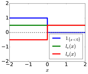
losseven function leodd function logenericl(x)12(l(x)+l(x))12(l(x)l(x))011{x0}112{x0}12sign(x)exponentialexcosh(x)sinh(x)hinge[1x]+12([1x]+[1x]+)12([1x]+[1+x]+)loll(x)12(l(x)+l(x))axρ-lossρ|x|ρx+1ρ|x|+1ρx(ρ0)unhinged1x1xperceptronmax(0,x)xsign(x)x2-hingemax(x,1/2max(0,1x))xsplal+l(x)/blal+12bl(l(x)+l(x))x/(2bl)logisticlog(1+ex)12log(2+ex+ex)x/2square(1x)21+x22xMatsushita1+x2x1+x2xmissing-subexpressionmissing-subexpressionmissing-subexpressionmissing-subexpressionlosseven function leodd function lomissing-subexpressionmissing-subexpressionmissing-subexpressionmissing-subexpressionmissing-subexpressionmissing-subexpressionmissing-subexpressionmissing-subexpressionmissing-subexpressionmissing-subexpressionmissing-subexpressionmissing-subexpressiongeneric𝑙𝑥12𝑙𝑥𝑙𝑥12𝑙𝑥𝑙𝑥missing-subexpressionmissing-subexpressionmissing-subexpressionmissing-subexpression011𝑥0112𝑥012sign𝑥missing-subexpressionmissing-subexpressionmissing-subexpressionmissing-subexpressionexponentialsuperscript𝑒𝑥𝑥𝑥missing-subexpressionmissing-subexpressionmissing-subexpressionmissing-subexpressionhingesubscriptdelimited-[]1𝑥12subscriptdelimited-[]1𝑥subscriptdelimited-[]1𝑥12superscriptsubscriptdelimited-[]1𝑥subscriptdelimited-[]1𝑥missing-subexpressionmissing-subexpressionmissing-subexpressionmissing-subexpressionlol𝑙𝑥12𝑙𝑥𝑙𝑥𝑎𝑥ρ-loss𝜌𝑥𝜌𝑥1𝜌𝑥1𝜌𝑥𝜌0unhinged1𝑥1𝑥perceptron0𝑥𝑥sign𝑥𝑥2-hinge𝑥1201𝑥𝑥splsubscript𝑎𝑙superscript𝑙𝑥subscript𝑏𝑙subscript𝑎𝑙12subscript𝑏𝑙superscript𝑙𝑥superscript𝑙𝑥𝑥2subscript𝑏𝑙logistic1superscript𝑒𝑥122superscript𝑒𝑥superscript𝑒𝑥𝑥2squaresuperscript1𝑥21superscript𝑥22𝑥Matsushita1superscript𝑥2𝑥1superscript𝑥2𝑥missing-subexpressionmissing-subexpressionmissing-subexpressionmissing-subexpression\begin{array}[]{|l|l|c|c|}\hline\cr\mbox{}&\mbox{loss}&\mbox{even function $l_{e}$}&\mbox{odd function $l_{o}$}\\ \hline\cr\hline\cr\hline\cr\mbox{generic}&l(x)&\frac{1}{2}(l(x)+l(-x))&\frac{1}{2}(l(x)-l(-x))\\ \hline\cr\mbox{01}&1\{x\leq 0\}&1-\frac{1}{2}\{x\neq 0\}&-\frac{1}{2}\operatornamewithlimits{sign}(x)\\ \hline\cr\mbox{exponential}&e^{-x}&\cosh(x)&-\sinh(x)\\ \hline\cr\mbox{hinge}&[1-x]_{+}&\frac{1}{2}([1-x]_{+}-[1-x]_{+})&\frac{1}{2}([1-x]_{+}-[1+x]_{+})^{\dagger}\\ \hline\cr\mbox{{lol}}&l(x)&\frac{1}{2}(l(x)+l(-x))&-ax\\ \mbox{$\rho$-loss}&\rho|x|-\rho x+1&\rho|x|+1&-\rho x\>\>(\rho\geq 0)\\ \mbox{unhinged}&1-x&1&-x\\ \mbox{perceptron}&\max(0,-x)&x~{}\mathrm{sign}(x)&-x\\ \mbox{2-hinge}&\max(-x,1/2\max(0,1-x))&\dagger\dagger&-x\\ \mbox{{spl}}&a_{l}+l^{\star}(-x)/b_{l}&a_{l}+\frac{1}{2b_{l}}(l^{\star}(x)+l^{\star}(-x))&-x/(2b_{l})\\ \mbox{logistic}&\log(1+e^{-x})&\frac{1}{2}\log(2+e^{x}+e^{-x})&-x/2\\ \mbox{square}&(1-x)^{2}&1+x^{2}&-2x\\ \mbox{Matsushita}&\sqrt{1+x^{2}}-x&\sqrt{1+x^{2}}&-x\\ \hline\cr\hline\cr\end{array}
Table 3: Factorization of losses in light of Theorem 12. The odd term of hinge loss is upperbounded by (1x)/21𝑥2(1-x)/2 in B. =max(x,1/2max(0,1x))+max(x,1/2max(0,1+x)){}^{\dagger\dagger}=\max(-x,1/2\max(0,1-x))+\max(x,1/2\max(0,1+x)).
Refer to caption
(a) 0-1 loss
Refer to caption
(b) Matsushita loss
Refer to caption
(c) ρ𝜌\rho-loss, ρ𝜌\rho=1
Refer to caption
(d) 2-hinge loss
Refer to caption
(e) hinge loss
Refer to caption
(f) Huber loss