All-electron self-consistent GW in the Matsubara-time domain: implementation and benchmarks of semiconductors and insulators

Abstract

The GW approximation is a well-known method to improve electronic structure predictions calculated within density functional theory. In this work, we have implemented a computationally efficient GW approach that calculates central properties within the Matsubara-time domain using the modified version of Elk, the full-potential linearized augmented plane wave (FP-LAPW) package. Continuous-pole expansion (CPE), a recently proposed analytic continuation method, has been incorporated and compared to the widely used Pade approximation. Full crystal symmetry has been employed for computational speedup. We have applied our approach to 18 well-studied semiconductors/insulators that cover a wide range of band gaps computed at the levels of single-shot G₀W₀, partially self-consistent GW₀, and fully self-consistent GW (scGW). Our calculations show that G₀W₀ leads to band gaps that agree well with experiment for the case of simple $s$-$p$ electron systems, whereas scGW is required for improving the band gaps in 3-$d$ electron systems. In addition, GW₀ almost always predicts larger band gap values compared to scGW, likely due to the substantial underestimation of screening effects. Both the CPE method and Pade approximation lead to similar band gaps for most systems except strontium titantate, suggesting further investigation into the latter approximation is necessary for strongly correlated systems. Our computed band gaps serve as important benchmarks for the accuracy of the Matsubara-time GW approach.

I Introduction

Calculations using density functional theoryKohn and Sham (1965); Hohenberg and Kohn (1964) (DFT) have become the standard ab initio technique to study the electronic and structural properties of molecules, nanoparticles, and periodic solids.Kohn et al. (1996); Dreizler and Gross (2012); Norskov et al. (2011); Ruiz et al. (2012) However, it is well-known that the electronic band gap of semiconductors and insulators is severely underestimated within DFT due to the lack of a derivative discontinuity in standard exchange-correlation potentials.Sham and Schlüter (1983) This deficiency hinders the theory’s useful application in fields such as optics, photovoltaics, thermoelectrics, and transport that require an accurate characterization of excited state properties.

The GW approximation, originally proposed by Hedin,Hedin (1965) provides a route to improve electronic descriptions and band gap results using many-body perturbation theory. The central quantity in this approach is the exchange-correlation self-energy ($\Sigma^{xc}$), which incorporates (i) the exact electronic exchange interaction, and (ii) the complex electron-electron correlation accounting for screening effects often treated within the random phase approximation (RPA).Eshuis et al. (2012); Ren et al. (2012) This approach has been applied to a wide variety of materials and provides electronic structure results in better agreement with experiments compared to its DFT counterpart.Chu et al. (2014); Yang et al. (2007); Shishkin and Kresse (2007); Kresse et al. (2012); Fuchs et al. (2007); Faleev et al. (2004)

Although studies employing the GW approximation have enjoyed early success in improving band gap predictions, many implementations rely on the pseudopotential (PP) approximation that treats pseudo wave functions and valence-core interactions at the level of DFT.Deslippe et al. (2012); Marini et al. (2001); Dixit et al. (2011); Pham et al. (2013) To avoid the PP approximation, several all-electron GW implementations have been reported in recent years based on the full-potential linearized augmented plane wave (FP-LAPW),Ku and Eguiluz (2002); Sharma et al. (2005); Friedrich et al. (2010); Jiang et al. (2013); Usuda et al. (2002) the linearized muffin-tin orbital (LMTO),Usuda et al. (2002) and the projector-augmented wave (PAW)Blöchl (1994) in conjunction with a plane-wave basis.Shishkin and Kresse (2006, 2007) Most of these all-electron studies have only implemented the G₀W₀ approximation due to its lower computational cost,Usuda et al. (2002); Gómez-Abal et al. (2008); Li et al. (2012) however these single-shot calculations are plagued by violations of momentum, energy, and particle conservation laws.Baym and Kadanoff (1961); Baym (1962); Dahlen et al. (2006) They also introduce a troubling dependence on the choice of Kohn-Sham (K-S) basis used as a zeroth order starting point.Rinke et al. (2005); Fuchs et al. (2007) Fully self-consistent GW (scGW) calculations avoid these issues and provide an unbiased physical picture predicted by GW theory. To date, few studies have performed scGW calculations within an all-electron framework,Caruso et al. (2012, 2013); Ku and Eguiluz (2002) among them includes the self-consistent GW method performed within the Matsubara-time domain,Mahan (2013); Bruus and Flensberg (2004); Ku and Eguiluz (2002) as first implemented by Ku and Eguiluz.Ku and Eguiluz (2002) However, this approach has only been applied to bulk Si and Ge and its applicability to other semiconductors and insulators requires further examination.

There are two main advantages of performing GW calculations within the Matsubara-time domain. First, $\Sigma$ is simply the product of the single-particle Green’s function ($G$) and screened Coulomb interaction ($W$). In contrast, the solution for $\Sigma$ in Matsubara-frequency space requires a convolution of $G$ and $W$ that usually demands more frequency points to reach convergence.Kutepov et al. (2009) Second, the Green’s function in Matsubara-time lacks singular points that can arise in frequency space, which leads to smoother single-particle Green’s functions compared to those in the frequency domain. Despite these advantages, the need for a reliable analytic continuation technique makes accurate calculations within Matsubara-time particularly challenging. The Pade approximation is often adopted for this purpose due to its simple implementation and low computational efficiency.Vidberg and Serene (1977) In this approach, the quantities of interest (e.g., $\Sigma$ and $G$) are expressed as fractional polynomials that are fitted to computed values in the Matsubara-frequency domain. Such expressions are then analytically continued into the real-frequency domain. The reliability of this approximation remains under debate, and recently Staar and co-workers have proposed the continuous-pole expansion (CPE) as an alternative algorithm for analytic continuation from the Matsubara-frequency to the real-frequency domain.Staar et al. (2014) Unlike the Pade approximation, this method explicitly takes into account the physical causality that places a constraint on the self-energy.

In this paper, we build upon an all-electron GW code we have already developedKozhevnikov et al. (2010); Chu et al. (2014) by calculating $\Sigma$ within the Matsubara-time domain, which improves the code’s computational efficiency and provides scGW calculations. We implement this method in conjunction with the CPE to solve for the quasiparticle energies in the real-frequency domain. We validate this method by investigating the electronic band gaps of a wide range of semiconductors and insulators at different levels of GW approximation. Our calculations demonstrate that the band gaps for 3-$d$ electron systems are often in better agreement with experiment when using scGW than the commonly used G₀W₀ approximation, whereas the latter approximation often yields reasonable experimental agreement in simple $s$-$p$ electron systems. We also find that both the CPE and Pade approximation yield very similar electronic band gaps among most tested systems, however the CPE method provides a better electronic description of strongly-correlated strontium titanate.

The rest of the paper is organized as follows. Section II outlines the scGW approximation and Section III describes its implementation within the existing all-electron DFT package. Results and discussion are then presented in Section V, followed by the conclusion in Section VI.

II Basics of the Theory

Within the single-particle picture, the excitation properties of solids can be determined by the single-particle Green’s function via Dyson equation. When expressed in real-space and Matsubara-time domain, the Dyson equation reads

$$G({\bf r},{\bf r}^{\prime}|\tau) =G^{0}({\bf r},{\bf r}^{\prime}|\tau)+\int^{\beta}_{0}d\tau_{1}\int^{\beta}_{0}d\tau_{2}\int d{\bf r}_{1}\int d{\bf r}_{2}G^{0}({\bf r},{\bf r}_{1}|\tau-\tau_{1})$$

$$\times\Delta\Sigma({\bf r}_{1},{\bf r}_{2}|\tau_{1}-\tau_{2})G({\bf r}_{2},{\bf r}^{\prime}|\tau_{2}),$$

where $G$ and $G^{0}$ are the Green’s functions associated with the interacting system of interest and a pre-selected reference system, respectively. In this work, the non-interacting K-S system calculated within DFT is adopted as the reference system. $\tau$ is the Matsubara-time argument that in general falls within [-$\beta$, $\beta$] where $\beta=1/k_{B}T$, $k_{B}$ is Boltzmann’s constant, and $T$ is the temperature. Given that $G$ obeys the relation $G({\bf r},{\bf r}^{\prime},-\tau)=-G({\bf r},{\bf r}^{\prime},-\tau+\beta)$ for $\tau\in[0,\beta]$, it is sufficient to restrict our study to $\tau\in[0,\,\beta$]. $\Delta\Sigma$ is the change in the electron-electron interaction between the interacting and reference K-S systems:

$$\Delta\Sigma({\bf r},{\bf r}^{\prime}|\tau)=\Sigma({\bf r},{\bf r}^{\prime}|\tau)-\Sigma^{0}({\bf r},{\bf r}^{\prime})\delta(\tau),$$ (2)

$$\Sigma({\bf r},{\bf r}^{\prime}|\tau)=\Sigma^{H}({\bf r})\delta({\bf r}-{\bf r}^{\prime})\delta(\tau)+\Sigma^{xc}({\bf r},{\bf r}^{\prime}|\tau),$$ (3)

$$\Sigma^{H}({\bf r})=\int d{\bf r}_{1}\frac{\rho({\bf r}_{1})}{|{\bf r}-{\bf r}_{1}|},$$ (4)

$$\rho({\bf r})=G({\bf r},{\bf r}|\tau\rightarrow 0^{-}).$$ (5)

Here, $\Sigma$ is the electron self-energy that captures the complicated electron-electron interactions. It is composed of the Hartree ($\Sigma^{H}$) and exchange-correlation ($\Sigma^{xc}$) components of the self-energy. $\Sigma^{H}$ relates to the updated electronic charge density ($\rho$) and $\Sigma^{0}$ is the sum of Hartree and exchange-correlation potentials in the reference K-S system. $\delta(\tau)$ is the Dirac delta function.

Given the high computational cost of calculating $\Sigma^{xc}$, the standard method used to find this quantity is the GW approximation, which can be expressed in real-space and Matsubara-time asMahan (2013)

$$\Sigma^{xc}({\bf r},{\bf r}^{\prime}|\tau)=-G({\bf r},{\bf r}^{\prime}|\tau)\cdot W({\bf r},{\bf r}^{\prime}|\tau).$$ (6)

Here, $W$ is the dynamically screened Coulomb potential, which describes the interactions between quasiparticles while including screening effects. The screened Coulomb potential obeys the Dyson equation that reads

$$W({\bf r},{\bf r}^{\prime}|\tau) =v({\bf r},{\bf r}^{\prime})\delta(\tau)+\int^{\beta}_{0}d\tau^{\prime}\int d{\bf r}_{1}\int d{\bf r}_{2}v({\bf r},{\bf r}_{1})$$

$$\times P({\bf r}_{1},{\bf r}_{2}|\tau-\tau^{\prime})W({\bf r}_{2},{\bf r}^{\prime}|\tau^{\prime}),$$

where $v({\bf r},{\bf r}^{\prime})=1/|{\bf r}-{\bf r}^{\prime}|$ is the bare Coulomb potential, and $P$ is the irreducible polarization within RPA,

$$P({\bf r},{\bf r}^{\prime}|\tau)=G({\bf r},{\bf r}^{\prime}|\tau)\cdot G({\bf r},{\bf r}^{\prime}|-\tau).$$ (8)

In addition, $\Sigma^{xc}(\tau)$ is often expressed as the sum of the exchange self-energy, $\Sigma^{x}(\tau)=-G(\tau)\cdot v\delta(\tau)$, which corresponds to the Fock exchange term, and the correlation self-energy, $\Sigma^{c}=-G(\tau)\cdot[W(\tau)-v\delta(\tau)]$. Note that the self-energy in Matsubara-time domain is simply a product of the Green’s function and screened Coulomb potential, in contrast to the corresponding expression in Matsubara-frequency domain that requires a convolution of $G$ and $W$. The electron self-energy within the GW approximation (its exchange-correlation part is given in Eq. (6)) correlates with the Green’s function and thus both need to be solved self-consistently via Eq. (II).

The set of inter-correlated equations presented above allows us to compute $G$ and $\Sigma$ self-consistently. Once they are converged to the required accuracy, a Fourier transform of $\Sigma$ from the Matsubara-time to Matsubara-frequency domain is performed, i.e. $\{\Sigma(\tau)\}\rightarrow\{\Sigma(i\omega_{n})\}$ where $\{\omega_{n}=(2n+1)\pi/\beta\}$ are the Matsubara frequencies with $n$ being integers, and the spatial dependence of $\Sigma$ is neglected for simplicity. This is then followed by an analytic continuation to real frequency space, $\{\Sigma(i\omega_{n})\}\rightarrow\{\Sigma(\omega+i\eta)\}$, with $\eta$ being a positive infinitesimal number, which yields the Green’s function in the real-frequency domain and the excitation spectrum of the system.

III Implementation of the Self-consistent GW Method

In this section, we describe the self-consistent GW approach in the Matsubara-time domain, which has been implemented in the modified version of the Elk FP-LAPW package.exc ; Kozhevnikov et al. (2010) The approach is essentially similar to the one proposed by Ku and Eguiluz,Ku and Eguiluz (2002) but with more efficient computational schemes. In particular, (i) we have employed the more efficient uniform power mesh (UPM) in Matsubara-time domain as proposed by Stan et al.,Stan et al. (2009) (ii) we have adopted the CPE for analytic continuation in conjunction with our scGW method, and (iii) full crystal symmetry has been taken into account to significantly reduce the computational load. We briefly summarize these improvements in the subsections below.

III.1 Matsubara-time sampling

The Green’s function $G$ in the Matsubara-time domain varies smoothly in the range $0\leq\tau\leq\beta$ and does not have any singularity points, however it varies rapidly near $\tau=0$ and $\beta$. To capture this behavior without losing computational efficiency, we employ the UPM to sample the $\tau$-axis on the grid $\{\tau_{0}=0,\tau_{1},\tau_{2},...,\tau_{M}=\beta\}$ as proposed by Stan et al.,Stan et al. (2009) which is a modified version of the original one by Ku and Eguiluz.Ku and Eguiluz (2002) The UPM grid can be characterized by a pair of integers ($p$, $m$) as well as the length of the interval $\beta$, in which $p$ is the number of non-uniform sub-intervals generated between 0 and $\beta$ with $2m-1$ evenly distributed grid points inside each of these sub-intervals. A UPM mesh with given ($p$, $m$) results in 2$pm$+1 grid points (including the end points) in the interval. In this scheme, the grid density increases for values of $\tau$ closer to the end points in order to capture the varying behavior of $G$. Using this scheme, explicit evaluation of quantities such as the self-energy and Green’s function, which is normally computationally expensive, now only requires a coarse UPM grid. Thus, implementation of this grid significantly reduces the computational effort. For $\tau$ domain integrals that require knowledge of the integrand on a dense uniform $\tau$ grid, e.g. solving the Dyson equation, a higher-order interpolation such as cubic spline can be subsequently applied.

III.2 Scheme for scGW in Matsubara-time domain

In this work, we expand and compute the Green’s function $G$ and self-energy $\Sigma$ using the K-S basis ({$\phi_{n{\bf k}}$}), whereas we evaluate the polarization function $P$ and the screened Coulomb potential $W$ in reciprocal space ({G}). We also assume that the quasiparticle wavefunctions are very similar to K-S eigenfunctions so that $\Sigma$ and $G$ become approximately diagonal in the K-S basis, significantly reducing computational effort. This approximation has been shown to provide reasonable results for a variety of systems.Shishkin and Kresse (2007); Usuda et al. (2002); Gómez-Abal et al. (2008) A direct generalization to include off-diagonal elements of $\Sigma$ is straightforward and will be completed in the future. The scGW approach is outlined below.

III.2.1 Green’s function in the reference K-S system $G^{0}$

As a first step in scGW, we construct the Green’s function in the reference K-S system ($G^{0}$):

$$G^{0}_{j}({\bf k}|\tau)=-\exp(-\epsilon_{j{\bf k}}\tau)[1-n_{F}(\epsilon_{j{\bf k}})],\ \ \ \ \ 0\leq\tau\leq\beta$$ (9)

where $\{\epsilon_{j{\bf k}}\}$ are the K-S eigenenergies measured from the chemical potential $\mu$ of the system, $n_{F}=[\exp(\beta\epsilon_{j{\bf k}})+1]^{-1}$ is the Fermi-Dirac distribution, and $\bf k$ is a wave vector. In the zero-temperature limit, the results for a system with a non-zero band gap are insensitive to the choice of $\mu$ provided that it is placed inside the gap.

III.2.2 Irreducible polarization

The irreducible polarization $P$ in the reciprocal space $\{{\bf G}\}$ can be obtained via Fourier transformations in Eq. (8) that reads,

$$P_{{\bf G}{\bf G}^{\prime}}({\bf q}|\tau)=\frac{1}{\Omega}\int d{\bf r}\int d{\bf r}^{\prime}e^{-i({\bf k}+{\bf G})\cdot{\bf r}}P({\bf r},{\bf r}^{\prime}|\tau)e^{i({\bf k}+{\bf G}^{\prime})\cdot{\bf r}^{\prime}},$$ (10)

where $\Omega$ is the volume of the unit cell, and ${\bf q}$ falling within the first Brillouin Zone (BZ). Using the relation between $P$ and $G$ in real space via Eq. (8), and by transforming the Green’s function from the Bloch-basis to real space,

$$G({{\bf r},{\bf r}^{\prime}}|\tau)=\sum^{BZ}_{{\bf k}}\sum_{j}\phi_{j{\bf k}}({\bf r})G_{j}({{\bf k}}|\tau)[\phi_{j{\bf k}}({\bf r}^{\prime})]^{*},$$ (11)

it is straight-forward to show that the irreducible polarization in the reciprocal space can be expressed as follows,

$$P_{{\bf G}{\bf G}^{\prime}}({\bf q}|\tau)=\frac{1}{\Omega N_{{\bf k}}}\sum_{\sigma}\sum^{BZ}_{{\bf k}}\sum_{j_{1},j_{2}}M^{{\bf k}}_{j_{2}j_{1}}({\bf G},{\bf q})Q_{j_{1}j_{2}}({\bf k},{\bf q}|\tau)[M^{\bf k}_{j_{2}j_{1}}({\bf G}^{\prime},{\bf q})]^{*},$$ (12)

$$Q_{j_{1}j_{2}}({\bf k},{\bf q}|\tau)=G_{j_{1}}({\bf k}+{\bf q}|\tau)G_{j_{2}}({\bf k}|-\tau),$$

$$M^{{\bf k}}_{nm}({\bf G},{\bf q})=\sum_{\sigma}\int d{\bf r}[\psi^{\sigma}_{n{\bf k}}({\bf r})]^{*}e^{-i({\bf q}+{\bf G})\cdot{\bf r}}\psi^{\sigma}_{m{\bf k}+{\bf q}}({\bf r}).$$ (13)

Here, $j_{1}$ and $j_{2}$ are dummy band indices that run through both valence and conduction bands, $\sigma$ is the dummy spin index, ${\bf q}$ is a reciprocal vector, and ${\bf G}$ is a reciprocal lattice vector. It is clear that the irreducible polarization $P$ at any two distinct $\tau_{1}$ and $\tau_{2}$ in [0, $\beta$] are decoupled. Therefore, parallelization over $\tau$ can be performed efficiently when $P$ is evaluated.

III.2.3 Screened Coulomb potential

The screened Coulomb potential ($W$) can be computed once $P$ is determined. Instead of directly solving for $W$, during which the emergence of the Dirac delta function $\delta(\tau)$ (see Eq. (II)) may lead to numerical instability, we work with $\tilde{W}(\tau)\equiv W(\tau)-v\delta(\tau)$ (only $\tau$ dependence is indicated for simplicity). This formulation yields a correlation self-energy, $\Sigma^{c}(\tau)=-G(\tau)\cdot\tilde{W}(\tau)$, and exchange self-energy, $\Sigma^{x}(\tau)=-G(\tau)v\cdot\delta(\tau)$, such that $\Sigma^{xc}(\tau)=\Sigma^{x}(\tau)+\Sigma^{c}(\tau)$. In reciprocal space and Matsubara-time domain, $\tilde{W}$ obeys the following Dyson equation

$$\tilde{W}_{{\bf G}{\bf G}^{\prime}}({\bf q}|\tau)= \sum_{{\bf G}_{2}}\left[\sum_{{\bf G}_{1}}v_{{\bf G}{\bf G}_{1}}({\bf q})P_{{\bf G}_{1}{\bf G}_{2}}({\bf q}|\tau)\right]v_{{\bf G}_{2}{\bf G}^{\prime}}({\bf q})$$ (14)

$$+\int^{\beta}_{0}d\tau^{\prime}\sum_{{\bf G}_{2}}\left[\sum_{{\bf G}_{1}}v_{{\bf G}{\bf G}_{1}}({\bf q})P_{{\bf G}_{1}{\bf G}_{2}}({\bf q}|\tau-\tau^{\prime})\right]\tilde{W}_{{\bf G}_{2}{\bf G}^{\prime}}({\bf q}|\tau^{\prime}),$$

where $v_{{\bf G}{\bf G}^{\prime}}({\bf q})=4\pi\delta_{{\bf G}{\bf G}^{\prime}}/|{\bf q}+{\bf G}|^{2}$ is the Fourier transform of the bare Coulomb potential. We follow the algorithm proposed by Stan et al.Stan et al. (2009) to discretize the $\tau$-axis using the generated UPM grid. The above equation can then be re-arranged to form a linear matrix equation that reads

$$\sum_{r=0}^{M}\sum_{{\bf G}_{2}}\left[\delta_{{\bf G}{\bf G}_{2}}\delta_{p,r}-A_{{\bf G}{\bf G}_{2}}({\bf q}|\tau^{(p)}-\tau^{(r)})\Delta\tau^{(r)}\right]\tilde{W}_{{\bf G}_{2}{\bf G}^{\prime}}({\bf q}|\tau^{(r)})$$

$$=\sum_{{\bf G}_{2}}A_{{\bf G}{\bf G}_{2}}({\bf q}|\tau^{(p)})v_{{\bf G}_{2}{\bf G}^{\prime}}({\bf q}),$$ (15)

$$A_{{\bf G}{\bf G}_{2}}({\bf q}|\tau)\equiv\sum_{{\bf G}_{1}}v_{{\bf G}{\bf G}_{1}}({\bf q})P_{{\bf G}_{1}{\bf G}_{2}}({\bf q}|\tau).$$

Here, the increments $\Delta\tau$ are positive, with $\Delta\tau^{(i)}=(\tau^{i+1}-\tau^{i-1})/2$ for $1\leq i\leq M-1$. At the end points, $\Delta\tau^{(0)}=(\tau^{1}-\tau^{0})/2$ and $\Delta\tau^{(M)}=(\tau^{M}-\tau^{M-1})/2$.

III.2.4 Evaluating the self-energy

With $\tilde{W}(\tau)$ and $G(\tau)$ in hand, the correlation self-energy ($\Sigma$) can be evaluated as

$$\Sigma^{c}_{n}({\bf k}|\tau)=-\frac{1}{\Omega N_{{\bf k}}}\sum^{BZ}_{{\bf q}}\sum_{{\bf G}{\bf G}^{\prime}}\sum_{j}\left[M^{{\bf k}-{\bf q}}_{jn}({\bf G},{\bf q})\right]^{*}O^{{\bf G}{\bf G}^{\prime}}_{j}({\bf k},{\bf q}|\tau)M^{{\bf k}-{\bf q}}_{jn}({\bf G}^{\prime},{\bf q}),$$ (16)

$$O^{{\bf G}{\bf G}^{\prime}}_{j}({\bf k}-{\bf q}|\tau)=G_{j}({\bf k}-{\bf q}|\tau)\tilde{W}({\bf q}|\tau).$$

On the other hand, the exchange self-energy $\Sigma^{x}$ is evaluated in real-space due to the slow convergence of $\Sigma^{x}$ in reciprocal space,Chu et al. (2014)

$$\Sigma^{x}_{n{\bf k}}=-\sum_{{\bf k}^{\prime}\in BZ}\sum^{occ}_{m}\int d{\bf r}\sum_{\sigma}[\psi^{\sigma}_{n{\bf k}}({\bf r})]^{*}\psi^{\sigma}_{m{\bf k}^{\prime}}({\bf r})\int d{\bf r}^{\prime}\frac{\sum_{\sigma}^{\prime}[\psi^{\sigma^{\prime}}_{m{\bf k}^{\prime}}({\bf r}^{\prime})]^{*}\psi^{\sigma^{\prime}}_{n{\bf k}}({\bf r}^{\prime})}{|{\bf r}-{\bf r}^{\prime}|}f_{m{\bf k}^{\prime}},$$ (17)

where $f_{j{\bf k}}=G_{j}({\bf k}|0^{-})$ is the occupation number of the K-S eigenfunction in spinor form, $\Psi_{j{\bf k}^{\prime}}({\bf r})=[\psi^{\uparrow}_{j{\bf k}}({\bf r}),\psi^{\downarrow}_{j{\bf k}}({\bf r})]$. Similarly, the Hartree potential is expressed as

$$\Sigma^{H}_{n{\bf k}}=\sum_{\sigma}\int d{\bf r}|\psi^{\sigma}_{n{\bf k}}({\bf r})|^{2}\int d{\bf r}^{\prime}\frac{\sum_{{\bf k}^{\prime}\in BZ}\sum_{\sigma^{\prime},m}|\psi^{\sigma}_{m{\bf k}^{\prime}}({\bf r}^{\prime})|^{2}}{|{\bf r}-{\bf r}^{\prime}|}f_{m{\bf k}^{\prime}}.$$ (18)

III.2.5 Dressed Green’s function

During the scGW calculation, the Green’s function ($G$) is updated in each iteration using the newly obtained self-energy $\Sigma$ in the Dyson equation, which reads

$$G^{N}_{j}({\bf k}|\tau)=G^{0}_{j}({\bf k}|\tau)+\int^{\beta}_{0}d\tau_{2}Z_{j{\bf k}}(\tau,\tau_{2})G^{N}_{j}({\bf k}|\tau_{2}),$$ (19)

$$Z_{j{\bf k}}(\tau,\tau_{2})=Z^{x}_{j{\bf k}}(\tau,\tau_{2})+Z^{c}_{j{\bf k}}(\tau,\tau_{2}),$$ (20)

$$Z^{x}_{j{\bf k}}(\tau,\tau_{2})=G^{0}_{j}({\bf k}|\tau-\tau_{2})[\Sigma^{x}_{N,j}({\bf k})+\Sigma^{H}_{N,j}({\bf k})-\Sigma_{0,j}({\bf k})],$$ (21)

$$Z^{c}_{j{\bf k}}(\tau,\tau_{2})=\int^{\beta}_{0}d\tau_{1}G^{0}_{j}({\bf k}|\tau-\tau_{1})\cdot\Sigma^{c}_{N,j}({\bf k}|\tau_{1}-\tau_{2}).$$ (22)

The integrals along the $\tau$ axis in Eqs. (19) and (22) may have substantial numerical errors when performed on the UPM mesh that becomes coarse farther away from the end points of $0\leq\tau\leq\beta$. To overcome this issue, a cubic spline interpolation is applied to the Green’s function and self-energy elements between two adjacent $\tau$ grid points, in which the increment $\Delta\tau$ in the resulting dense uniform $\tau$ grid is selected as $\tau_{1}-\tau_{0}$. This is also the smallest $\Delta\tau$ in the UPM mesh. Then the Dyson equation is solved on the generated, denser uniform $\tau$ mesh. Similar to the algorithm for $\tilde{W}$ as proposed by Stan et al.,Stan et al. (2009) the Dyson equation for $G$ along $\tau$ axis can be re-arranged to form a linear matrix equation.

$$\sum^{N}_{r=1}[\delta_{p,r}-\Delta\tau^{(r)}Z_{j{\bf k}}(\tau^{(p)},\tau^{(r)})]G^{N}_{j}({\bf k}|\tau^{(r)})=G^{0}_{j}({\bf k}|\tau^{(p)}).$$ (23)

During the scGW calculation, we repeat the steps mentioned above in each iteration using the newly obtained Green’s function $G$, as indicated in Eqs.(12), (15)-(18) and (21)-(23). We solve for the self-energy and the Green’s function in Matsubara-time domain self-consistently until any given accuracy is reached. Note that this corresponds to the single-shot G₀W₀ if the self-consistent calculation is terminated at the first iteration. The approximated calculation known as GW₀ can also be performed if the screened Coulomb potential $W$ is kept constant after the first iteration whereas $G$ is updated during the self-consistent loop.

III.2.6 Analytic continuation

To obtain quantities that can be measured in experiments, such as the excitation spectrum, knowledge of $G$ and $\Sigma$ in the real-frequency domain is required. This is achieved by a two-step procedure performed after calculating the converged self-energy in the Matsubara-time domain ($\Sigma^{xc}(\tau)$). First, a Fourier transformation from Matsubara-time to Matsubara-frequency domain is employed. For a given band index $n$ and ${\bf k}$, this reads

$$\Sigma^{xc}_{j}({\bf k}|i\omega_{n})=\int^{\beta}_{0}d\tau e^{i\omega_{n}\tau}\Sigma^{xc}_{j}({\bf k}|\tau),$$ (24)

where $\omega_{n}=(2n+1)\pi/\beta$ is the Matsubara frequency with $n$ being an integer. We use a cubic spline interpolation of the UPM grid for the accurate evaluation of the integral. Second, we implement analytic continuation using the CPE method proposed by Staar et al.Staar et al. (2014) to yield the self-energy in the real-frequency domain ($\Sigma^{xc}(\omega+i\eta)$). Unlike the commonly used Pade approximation,Vidberg and Serene (1977) where the self-energy elements are simply expanded as polynomials, the CPE takes advantage of the fact that the self-energy in the upper complex plane ($z$) can be expressed as

$$\Sigma_{j}^{xc}({\bf k},z)=\frac{1}{2\pi}\int^{+\infty}_{-\infty}d\omega\frac{\operatorname{Im}[\Sigma^{xc}_{j}({\bf k},\omega+i\eta)]}{\omega-z},$$ (25)

$$\operatorname{Im}[\Sigma^{xc}_{j}({\bf k},\omega+i\eta)]<0,$$ (26)

where $\eta$ is a positive infinitesimal and Eq. (26) arises from causality. For each $j$ and ${\bf k}$, $\operatorname{Im}\Sigma^{xc}_{j}({\bf k}|\omega+i\eta)$ can be expanded as a set of piecewise linear functions of $\omega$ with undetermined coefficients $\{a_{nj}({\bf k})\}$. This leads to $\Sigma^{xc}_{j}({\bf k},z)=\sum_{m}a_{mj}({\bf k})\Phi_{mj,{\bf k}}(z)$ where $\Phi_{mj,{\bf k}}(z)$ is some analytic function defined in the upper complex plane $z$. With the set of computed elements $\{\tilde{\Sigma}^{xc}_{j}({\bf k}|i\omega_{m})\}$ in hand and Eq. (26) as the constraint, for each given $j$ and ${\bf k}$, $\{a_{nj}({\bf k})\}$ are then determined by minimizing the norm function $\Omega$ defined as

$$\Omega_{j}({\bf k})=\sum^{M}_{m=0}|\tilde{\Sigma}^{xc}_{j}({\bf k}|i\omega_{m})-\Sigma^{xc}_{j}({\bf k}|i\omega_{m})|^{2},$$ (27)

with $M$ being the number of positive Matsubara frequencies. Given the fitted $\Sigma_{j}^{xc}({\bf k}|\omega)$, for each $j$ and ${\bf k}$, the Green’s function associated with the interacting system can be determined using

$$G_{j}({\bf k}|\omega)=\frac{1}{[G^{0}_{j}({\bf k}|\omega)^{-1}-\Sigma^{xc}_{j}({\bf k}|\omega)-\Sigma^{H}_{j}({\bf k})]}.$$ (28)

The quasiparticle energies, and hence the electronic band gap can be directly obtained from the spectral function $A_{j{\bf k}}(\omega)=-\frac{1}{\pi}$Im$[G_{j{\bf k}}(\omega)]$ for given $j$ and ${\bf k}$.

III.3 Use of Crystal Symmetry for Computational Speedup

Calculating the elements of $\Sigma^{c}(\tau)$ can be computationally expensive as it involves the evaluation of Eqs. (12), (13), (15) and (16). Such computational effort can be considerably reduced using crystal symmetry to decrease the number of required operations. The allowed crystal symmetry operations are those that leave the Hamiltonian invariant. Using these operations, reciprocal vectors in the first BZ $\{{\bf k}_{BZ}\}$ are decomposed to a number of subsets. The reciprocal vectors in each of these subsets are related via the action of the symmetry operations. Therefore, the first BZ can be represented using a reduced set of ${\bf k}$ vectors that form the irreducible BZ, denoted as $\{{\bf k}_{IBZ}\}$.

Suppose $S_{u}\equiv\{({\bf R}_{i}|{\bf t}_{i}),i=1,...,N_{u}\}$ is the set of symmetry operations in which ${\bf R}$ is a $3\times 3$ rotation matrix and ${\bf t}$ the translation vector in real space. The application of a given symmetry operation, $B_{i}=({\bf R}_{i}|{\bf t}_{i})$, on the real-space vector ${\bf r}$ and reciprocal vector in IBZ lead respectively to

$$B_{i}{\bf r}={\bf R}_{i}{\bf r}+{\bf t}_{i},$$ (29)

$${\bf k}_{BZ}=B_{i}{\bf k}_{IBZ}={\bf R}_{i}{\bf k}_{IBZ}+{\bf G}_{{\bf R}i},$$ (30)

where ${\bf G}_{{\bf R}i}$ is the reciprocal lattice vector that brings ${\bf R}_{i}{\bf k}_{IBZ}$ back to the 1st BZ. For a given ${\bf q}_{BZ}$ that is associated with ${\bf q}_{IBZ}$ via ${\bf R}$ and ${\bf G}$ using Eq. (30), it is straight forward to prove that the plane-wave matrix $M$ in Eq.(13), the irreducible polarization $P(\tau)$ in Eq.(12), and $\tilde{W}(\tau)$ in Eq.(15) obey the following relations

$$M^{{\bf k}}_{nm}({\bf G},{\bf q}_{BZ})=M^{{\bf R}^{-1}{\bf k}}_{nm}[{\bf G}_{1},{\bf q}_{IBZ}]\exp[-i({\bf R}{\bf q}_{IBZ}+{\bf G}_{{\bf R}}+{\bf G})\cdot{\bf t}],$$ (31)

$$P_{{\bf G}{\bf G}^{\prime}}({\bf q}_{BZ}|\tau)=P_{{\bf G}_{1}{\bf G}^{\prime}_{1}}({\bf q}_{IBZ}|\tau)\exp[-i({\bf G}-{\bf G}^{\prime})\cdot{\bf t}],$$ (32)

$$\tilde{W}_{{\bf G}{\bf G}^{\prime}}({\bf q}_{BZ}|\tau)=\tilde{W}_{{\bf G}_{1}{\bf G}^{\prime}_{1}}({\bf q}_{IBZ}|\tau)\exp[-i({\bf G}-{\bf G}^{\prime})\cdot{\bf t}],$$ (33)

where ${\bf G}_{1}={\bf R}^{-1}({\bf G}+{\bf G}_{{\bf R}})$ and ${\bf G}^{\prime}_{1}={\bf R}^{-1}({\bf G}^{\prime}+{\bf G}_{{\bf R}})$. It follows that the correlation self-energy can be re-arranged as

$$\Sigma^{c}_{n}({\bf k}|\tau)= -\frac{1}{\Omega N_{{\bf k}}}\sum_{{\bf q}_{IBZ}}\sum_{{\bf R}}\sum_{{\bf G}{\bf G}^{\prime}}\tilde{W}_{{\bf G}{\bf G}^{\prime}}({\bf q}_{IBZ}|\tau)\sum_{j}[M^{{\bf R}^{-1}{\bf k}-{\bf q}_{IBZ}}_{jn}({\bf G},{\bf q}_{IBZ})]^{*}$$ (34)

$$\times G_{j}({\bf R}^{-1}{\bf k}-{\bf q}_{IBZ}|\tau)M^{{\bf R}^{-1}{\bf k}-{\bf q}_{IBZ}}_{jn}({\bf G}^{\prime},{\bf q}_{IBZ}).$$

Here, ${\bf R}^{-1}{\bf k}-{\bf q}_{IBZ}$ is assumed to fall in the set of $\{{\bf k}_{BZ}\}$ vectors. It is thus sufficient to compute the summands in the above equation for the sets of $\{{\bf q}_{IBZ}\}$ and $\{{\bf k}_{BZ}\}$ vectors, which leads to significant reduction to computational time. Similarly, the computation of the elements of $\Sigma^{x}$ can be sped up with the use of symmetry operations for ${\bf k}$. According to Eq. (17), in particular, ${\bf k}$ associated with $\Sigma^{x}$ can be confined to the IBZ, whereas ${\bf k}^{\prime}$ runs over the 1st BZ.

IV Computational Details

The scGW scheme has been applied to calculate the electronic band gaps of 18 diverse semiconductors and insulators. We have adopted the experimental lattice parameters of 5.43 $\AA$ (Si), 5.658 $\AA$ (Ge), 5.66 $\AA$ (GaAs), 4.35 $\AA$ (SiC), 5.91 $\AA$ (CaSe), 3.57 $\AA$ (diamond), 5.64 $\AA$ (NaCl), 4.21 $\AA$ (MgO), 3.62 $\AA$ (cubic BN), 4.01 $\AA$ (LiF), 3.91 $\AA$ (cubic SrTiO3), 4.27 $\AA$ (Cu2O), 4.52 $\AA$ (GaN), 4.58 $\AA$ (zinc-blende ZnO), 5.42 $\AA$ (zinc-blende ZnS), 5.67 $\AA$ (zinc-blende ZnSe), 6.05 $\AA$ (zinc-blende CdSe) and 5.82 $\AA$ (zinc-blende CdS) throughout this work. All DFT calculations have been carried out using the modified version of the Elk FP-LAPW package.exc ; Kozhevnikov et al. (2010) The augmented plane wave + local orbitals (APW+lo) basisSjöstedt et al. (2000) with a single second-order local orbital per core or semi-core state has been adopted. The local density approximation (LDA)Perdew and Wang (1992) has been utilized for the exchange-correlation functionals. When expanding the interstitial potential and charge density, the maximum length of the reciprocal lattice vector $|{\bf G}|$ has been chosen as 12 a.u. The angular momentum has been truncated as $\ell_{max}=8$ for the expansions of muffin-tin charge density, potential and wave function. In the expansion of the wave function, $|{\bf G}+{\bf k}|_{max}=8.0/R_{avg}$ has been used, where $R_{avg}$ is the average of the muffin-tin radii ($R^{MT}$) in each system. Linearization energy ($E_{\ell,\nu}$), which is associated with each radial function labeled with $\nu$, is chosen at the center of the corresponding band with $\ell$-like character. The first BZ has been sampled by a $4\times 4\times 4$ ${\bf k}$-mesh for all the systems except for diamond, where a $6\times 6\times 6$ ${\bf k}$ mesh has been used instead. All the aforementioned parameters have been carefully tested to achieve total energy convergence.

In the GW calculations, the cutoff for $|{\bf G}+{\bf q}|$ used in Eqs. (12) and (18) has been set 4.0 a.u. for all the systems except for the systems of ZnO, diamond and cubic BN (c-BN), where a cutoff of 5.0 a.u. has been selected instead. These length cutoffs correspond to a kinetic-energy cutoff of 16 Ry and 25 Ry, respectively. The Matsubara-time ($\tau$) domain has been sampled with a (9, 5) UPM mesh, which consists of 81 grid points between 0 and $\beta$ associated with an artificial temperature of 300 K. A minimum of 150 conduction bands have been included for the band summations in Eqs. (12) and (18) for the systems studied to ensure the convergence of the band gaps. In the GW₀ and scGW calculations, states with an energy falling in the energy window of $\pm$ 15 eV around the DFT-LDA Fermi energy have been updated, and the number of iterations has been set 4. In the transformation indicated in Eq. (24), a set of 128 positive Matsubara frequencies has been adopted, which is subsequently used in analytic continuation schemes of both CPE and Pade approximation. For comparison, we have also performed G₀W₀ calculations using the plasmon-pole approximation (PPA), in which we have selected the model proposed by Godby and NeedsGodby and Needs (1989) that has proven to be in consistent agreement with numerical integration method.Stankovski et al. (2011); Chu et al. (2014) All the above parameters are carefully examined to ensure the band gap values converged to within 50 meV.

V Results and Discussion

V.1 Benchmarking Si, Ge and GaAs

We first apply the Matsubara-time GW method to study the electronic properties of bulk silicon (Si), a prototypical system that has been studied as a benchmark for previous GW code developments. Figure 1(a) and (b) illustrate the Matsubara-time Green’s functions ($G(\tau)$) of the band-edge states at $\Gamma_{v}$ and $X_{c}$ at different levels of GW approximations, where $K_{v}$ ($K_{c}$) denotes the highest occupied (lowest unoccupied) single-particle state at $K$. $G(\tau)$ approaches -1 and 0 at each end of the $\tau$ axis. For the case of the valence (conduction) band state in a semiconductor/insulator, $G(\beta^{-})\rightarrow-1(0)$ to account for the occupation number of that state. It can be seen that in Matsubara-time domain, scGW leads to substantial changes of $G$ compared to those from G₀W₀. It is worth pointing out that the dressed $G$ at $\Gamma_{v}$ upon scGW becomes very similar to that from LDA, i.e. $G^{0}$. On the other hand, the scGW leads to more deviation of $G$ at $X_{c}$ from $G^{0}$, suggesting that GW corrections to the conduction bands are likely more pronounced than to the valence bands. Figure 1 (c) shows the typical Green’s function in Matsubara-frequency domain (both real and imaginary parts) for the band edge states of bulk Si from scGW calculations.

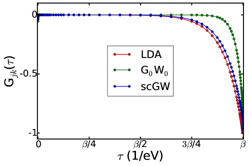
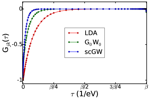
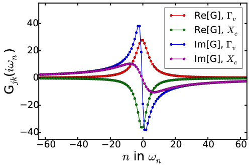
Figure 1: (Color online) Single-particle Green’s functions $G_{n{\bf k}}$ at the (a) valence band maximum ($\Gamma_{v}$) and (b) conduction band minimum ($X_{c}$) of bulk Si in Matsubara-time domain. (c) Single-particle Green’s function of bulk Si in Matsubara-frequency domain from scGW calculations.

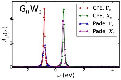
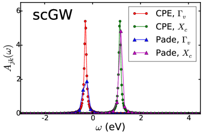
Figure 2: (Color online) Spectral functions of band edge states $\Gamma_{v}$ and $X_{c}$ of bulk Si from (a) G₀W₀, and (b) scGW. Spectral functions of band edge states $R_{v}$ and $\Gamma_{c}$ of SrTiO3 from (c) G₀W₀, and (d) scGW.

The calculated band gaps for bulk Si are tabulated in Table 1. When the non-self-consistent G₀W₀ calculation is performed, the direct band gap at $\Gamma$ and the indirect band gap from $\Gamma$ to $X$ are, respectively, 3.40 eV and 1.38 eV. These values are in relatively good agreement with experimental values.Landolt-Börnstein (1987) Compared to those obtained from plane-wave pseudopotential (PP)-based and/or all-electron G₀W₀, our computed G₀W₀ direct band gap and the indirect band gap are 0.1 eV and 0.2 eV higher, respectively. Moreover, we notice that band gap values are further increased by 0.2 eV upon implementing the partially self-consistent, GW₀ calculation. However, fully self-consistent GW brings the direct and indirect band gap values close to those calculated within the G₀W₀ approximation. Our scGW results are also comparable with the previous study by Ku et al., which uses a similar implementation to the present method. We also compare the results at different levels of GW using either the CPE method or Pade approximation. Band gap results using the Pade approximation generally agree well with those using CPE analytic continuation within 0.02 eV. However, the Si direct band gap value predicted by the Pade approximation is 0.16 eV higher than the CPE value, and is 0.09 eV higher than the value by Ku et al.. This also shows that CPE results are generally in better agreement with experiment. In addition, all levels of GW calculations, from G₀W₀ to scGW, overestimate the experimental indirect band gap value by 0.13 to 0.34 eV. The overestimation arising by scGW also agrees with the previous GW study.Shishkin and Kresse (2007)

Note that the important effect of core electrons on the valence-core interaction, and hence exchange self-energy has been discussed for bulk Si in the previous study.Ku and Eguiluz (2002) We have also evaluated the exchange self-energy elements of band edge states $\Gamma_{v}$ and $X_{c}$ with and without the core electrons. The difference in self-energy can be as large as 2 eV, in line with values given in that study.

We have also compared the spectral functions ($A_{j{\bf k}}(\omega)$) of the band edge states $\Gamma_{v}$ and $X_{c}$ of bulk Si from CPE to those obtained from Pade approximation, as shown in Figure 2 (a) and (b) for the cases of G₀W₀ and scGW, respectively. In the case of Si, results from these two approaches of analytic continuation are very similar in terms of peak position, as well as the broadening of peaks that is related to the lifetime of the associated quasiparticle states.

Table 1: Band gap values of bulk Si for various levels of approximation. The values in parentheses are computed using the Pade approximation. All values are in eV.

	$\Gamma_{v}-\Gamma_{c}$	$\Gamma_{v}-X_{c}$
This work
LDA	2.52	0.58
G0W0	3.40 (3.38)	1.38 (1.36)
GW0	3.69 (3.68)	1.59 (1.58)
scGW	3.41 (3.57)	1.44 (1.44)
plane-wave PP, G0W0a	3.24	1.18
all-electron, G0W0
Hamada et al.b	3.30	1.14
Kotani et al.c	3.13
Ku et al.d	3.12
Gomez-Abal et al.e		1.15
all-electron, scGWd	3.48
Experimentf	3.35	1.25

• Reference Tiago et al., 2004.

• Reference Hamada et al., 1990.

• Reference Kotani and van Schilfgaarde, 2002.

• Reference Ku and Eguiluz, 2002.

• Reference Gómez-Abal et al., 2008.

• Reference Landolt-Börnstein, 1987.

Finally, we demonstrate the computational advantage of the current implementation by evaluating silicon’s G₀W₀ band gaps with a similar parameter set but using a direct numerical integration method in the real-frequency domain. We find that more than 1000 frequency points are needed to achieve the converged results. Since the computational load at each frequency/Matsubara-time grid point is similar, it is clear that significant computational speedup can be accomplished when GW calculation is performed in Matsubara-time domain (81 $\tau$ points used in this work).

Table 2: Band gap values of bulk Ge for various levels of approximation. The values in parentheses are computed using the Pade approximation. All values are in eV.

	$\Gamma_{v}-\Gamma_{c}$	$\Gamma_{v}-L_{c}$	$\Gamma_{v}-X_{c}$
This work
LDA	-0.19	0.03	0.64
G0W0	0.49 (0.51)	0.58 (0.59)	0.65 (0.70)
GW0	1.09 (1.10)	0.85 (0.86)	1.35 (1.33)
scGW	1.11 (1.11)	0.85 (0.85)	1.30 (1.30)
plane-wave PP, G0W0a	0.85	0.65	0.98
all-electron, G0W0
Kotani et al.b	0.89	0.57
Ku et al.c	1.11	0.51	0.49
all-electron, scGWc	1.51	0.79	0.71
Experimentd	0.90	0.74	1.30

• Reference Tiago et al., 2004.

• Reference Kotani and van Schilfgaarde, 2002.

• Reference Ku and Eguiluz, 2002.

• Reference Landolt-Börnstein, 1987.

Table 2 summarizes the band gaps at different levels of theory for bulk Ge. The minimal, indirect band gap of bulk Ge is between $\Gamma_{v}$ and $L_{c}$ according to experiment.Landolt-Börnstein (1987) It is clear that both LDA and G₀W₀ predict a minimal band gap as direct at $\Gamma$, inconsistent with experiment. It is only when the self-consistency is considered in GW, (either GW₀ or scGW) that the correct indirect band gap can be predicted. Note that the results from scGW agree well with experimental data, and also very close to those from GW₀, regardless of CPE or Pade approximation being adopted. It is worth pointing out that there is a substantial difference between our results and those by Ku et al., with a band gap difference as large as 0.5 eV. We believe that such discrepancy is due mainly to the insufficient amount of empty bands used in their study, as pointed out in the previous study by Tiago et al..Tiago et al. (2004)

Table 3: Band gap values of bulk GaAs for various levels of approximation. The values in parentheses are computed using the Pade approximation. All values are in eV.

	$\Gamma_{v}-\Gamma_{c}$	$\Gamma_{v}-L_{c}$	$\Gamma_{v}-X_{c}$
This work
LDA	0.23	0.81	1.31
G0W0	1.48 (1.47)	1.62 (1.62)	1.98 (1.94)
GW0	1.82 (1.83)	2.00 (2.00)	2.31 (2.30)
scGW	1.80 (1.81)	1.95 (1.96)	2.23 (2.25)
plane-wave PP, G0W0a	1.38	1.65	1.83
all-electron, G0W0
Kotani et al.b	1.20	1.40	1.46
Gomez-Abal et al.c	1.29
Friedrich et al.d
Experimente	1.52	1.82	1.98

• Reference Tiago et al., 2004.

• Reference Kotani and van Schilfgaarde, 2002.

• Reference Gómez-Abal et al., 2008.

• Reference Friedrich et al., 2010.

• Reference Aspnes, 1976.

Gallium aresnide is another common compound we use as a benchmark, with computed band gap results shown in Table 3. This compound has also been extensively investigated, which has a direct electronic band gap at $\Gamma$. Our calculations show that G₀W₀ results in the best agreement with experiment,Aspnes (1976) and also agree with previous all-electron G₀W₀ studies with a $\sim$0.2 eV difference. Moreover, both scGW and GW₀ lead to larger band gap values compared to the G₀W₀ results, and are overestimated by around 0.3 eV compared to experiment. Such trends regarding G₀W₀ and scGW are also in line with previous GW studies within the plane-wave PAW potential framework.Shishkin and Kresse (2007) Similar to the aforementioned compounds investigated, the CPE and Pade approximation lead to very close results to each other. Our scGW results presented here also serve as important predictions for this level of theory since there are no previous all-electron-based, self-consistent GW results for GaAs.

In general, G₀W₀ accurately predicts Si and GaAs band gap values but predicts inaccurate bulk Ge band gap values compared to experiment. On the other hand, scGW band gaps agree fairly well with experiment across all three elements, and GW₀ generally worsens the band gaps compared to scGW.

V.2 Band gap calculations for other semiconductors and insulators

Having demonstrated the accuracy of scGW calculations for predicting electronic band gaps in benchmark materials, we next report results for 18 semiconductors/insulators that have band gaps covering a wide range of values from less than 1 eV to over 10 eV. The calculated minimal band gaps are summarized in Table 4, comparing all levels of approximation, and also in Fig. 3 which visualizes LDA, G₀W₀, and scGW results. As expected, the LDA band gaps are always severely underestimated compared to experimental values. Upon GW corrections, the electronic band gaps for all the systems studied are substantially improved. In the following, we discuss the effects of G₀W₀ and scGW band gap corrections by categorizing the compounds studied into three groups: (1) simple $s$-$p$ electron systems involving Si, SiC, C, BN, LiF, NaCl and MgO; (2) non-transition-metal systems with 3-$d$ electrons that include Ge, GaAs, GaN, CaSe, CdSe and CdS; and (3) transition-metal chalcogenides of SrTiO3, Cu2O, ZnO, ZnS, ZnSe.

Table 4: Electronic band gap (in eV) of various semiconductors and insulators calculated by DFT-LDA, different levels of Matsubara-time GW (G₀W₀, GW₀ and scGW), and PPA-G₀W₀. Values in the parentheses are obtained using the Pade approximation. The experimental values (Expt.) are also given for comparison.

	LDA	G0W0	GW0	full-GW	PPA-G0W0	Expt.
Si	0.58	1.38 (1.36)	1.59 (1.58)	1.44 (1.44)	1.28	1.25a
Ge	0.03	0.58 (0.59)	0.85 (0.86)	0.85 (0.85)	0.71	0.74a
GaAs	0.24	1.48 (1.47)	1.82 (1.83)	1.80 (1.81)	1.51	1.52b
SiC	1.27	2.44 (2.45)	2.90 (2.90)	2.64 (2.56)	2.30	2.40a
CaSe	2.00	3.89 (3.94)	4.60 (4.64)	4.35 (4.34)	3.89	3.85c
C	4.14	6.15 (6.15)	6.42 (6.43)	6.10 (6.11)	6.09	5.48a
NaCl	4.74	8.09 (8.11)	9.00 (9.02)	8.27 (8.28)	8.11	8.5d
MgO	4.65	7.79 (7.78)	8.74 (8.74)	7.94 (7.94)	7.75	7.83e
BN	4.34	6.71 (6.73)	7.16 (7.18)	7.10 (7.11)	6.58	6.1-6.4f
LiF	8.94	14.51 (14.54)	15.78 (15.81)	14.45 (14.47)	14.55	14.20g
SrTiO3	1.75	3.58 (4.08)	7.01 (7.13)	6.87 (7.22)	3.86	3.25h
Cu2O	0.52	1.61 (1.54)	2.16 (2.17)	2.00 (2.02)	1.59	2.17i
GaN	1.70	3.01 (3.05)	3.61 (3.66)	3.36 (3.38)	3.03	3.27j
ZnO	0.60	2.31 (2.35)	3.69 (3.71)	3.53 (3.56)	2.32	3.44k
ZnS	1.80	3.46 (3.43)	4.06 (4.09)	3.92 (3.85)	3.43	3.91k
ZnSe	1.01	2.43 (2.48)	3.03 (3.09)	2.94 (2.96)	2.50	2.95a
CdSe	0.34	1.42 (1.51)	1.97 (1.98)	1.92 (1.93)	1.46	1.83a
CdS	0.86	2.01 (2.03)	2.63 (2.66)	2.49 (2.50)	2.06	2.50a

• Reference Landolt-Börnstein, 1987.

• Reference Aspnes, 1976.

• Reference Kaneko and Koda, 1988.

• Reference Poole et al., 1975.

• Reference Whited et al., 1973.

• Reference Lev, 2001.

• Reference Piacentini et al., 1976.

• Reference van Benthem et al., 2001.

• Reference Baumeister, 1961.

• Reference Okumura et al., 1994.

• Reference Kittel and McEuen, 1986.

Figure 3: (Color online) Computed electronic band gap at DFT-LDA as well as GW levels versus the experimental counterpart for all the compounds studied in this work except for Ge. Log scale is adopted for both axes.

Concerning simple $s$-$p$ electron systems, the G₀W₀ corrected band gaps are in very good agreement with experimental data, with a relative band gap error of $\pm 10\%$ for most compounds with the exception of diamond, for which G₀W₀ overestimates the experimental gap by 0.6 eV ($12\%$). This may be attributed to the RPA that leads to more severe underestimation of the screening effect in diamond, as pointed out in a previous study.Shishkin and Kresse (2007) Results using PPA are remarkably close to general G₀W₀ calculations, differing by only 0.1 eV or less. Our G₀W₀ band gaps are all comparable to previous all-electron G₀W₀ calculations.Friedrich et al. (2010); Gómez-Abal et al. (2008) When full self-consistency is taken into account, our calculations show that scGW may further overestimate the electronic band gap due probably to the underestimated screening effect by RPA, in agreement with previous findings.Shishkin and Kresse (2007); Shishkin et al. (2007) The exceptions are diamond and the ionic crystals NaCl and LiF, for which the inclusion of self-consistency tends to improve results. It is worth pointing out that the band gaps from partially self-consistent GW₀ are considerably higher than scGW ones, which is in contrast to previous finding.Shishkin and Kresse (2007) This different trend is likely due to differences in method implementation. Specifically, the Green’s function in our approach is fully updated during the GW₀ iteration, whereas in the previous GW₀ study only the shift in quasiparticle energies is updated in the Green’s function.Shishkin and Kresse (2007) Compared to our scGW results, the further overestimation of GW₀ band gaps can be attributed to the further underestimation of screening due to the screened potential ($W$), which is not updated iteratively within GW₀. This also highlights the importance of the full self-consistency. Furthermore, the band gaps at different levels of GW have also been computed based on the CPE and Pade approximation. According to our results, they are in remarkable agreement with each other, with a typical difference of 0.1 eV or less in all the cases. This also confirms the applicability of the Pade approximation and the analytic continuation approach for $s$-$p$ electron systems.

For non-transition-metal systems with 3-$d$ electrons, we have observed that G₀W₀ corrected band gaps are typically still underestimated. Fully self-consistent GW calculations are necessary to achieve better agreement with experimental data. The exception involves CaSe and GaAs, in which scGW leads to overestimated band gaps of about 0.3-0.5 eV, corresponding to a relative difference of more than 12 %. Compared to scGW, GW₀ results in about 5 % larger band gap values in the systems studied. The difference is smaller than in the case of $s$-$p$ electron systems.

Moreover, in the cases of transition metal chalcogenides ZnO, ZnS and Cu2O, it is clear that band gaps resulting from G₀W₀ are substantially underestimated by at least 0.5 eV compared to the experimental values. In particular, the G₀W₀ band gap of ZnO is 1 eV lower than the experimental data, agreeing well with previously underestimated values.Shishkin and Kresse (2007) Upon scGW, the band gaps of these systems are significantly improved such that they are within 0.2 eV of experimental results. In the case of the perovskite SrTiO3, on the other hand, our G₀W₀ approach overestimates the band gap by about 0.3 eV, which is also consistent with the studies by Friedrich et al.Friedrich et al. (2010) and Kang et al.,Kang et al. (2015) and both scGW and GW₀ worsen the band gap prediction further with a result of more than 6.8 eV, much higher than the experimental value of 3.25 eV. We have further varied parameters such as the number of conduction bands and the cutoff of reciprocal lattice vectors, and the corresponding results only change slightly.

A previous GW study by Cappellini et al. also showed that the minimal band gap of SrTiO3 can be severely overestimated even at the level of G₀W₀ (5.07 eV),Cappellini et al. (2000) Such an overestimation may be attributed to the improper description of local field effects by their model dielectric function. Moreover, our scGW band gap of SrTiO3 is indeed in line with the previous findings, in which the band gap is overestimated by around 0.9 eV in all-electron quasiparticle self-consistent GW,van Schilfgaarde et al. (2006) whereas such overestimation becomes 1.8 eV in self-consistent GW with the diagonal approximation in the plane-wave PAW potential framework.Kang et al. (2015) Such a severe overestimation of the calculated scGW band gap is thus likely due to the poor accuracy of the diagonal approximation adopted for $G$, which leads to unchanged charge and spin densities during scGW. For systems with strongly correlated 3-$d$ electrons near the band edge, such as SrTiO3, the quasiparticle wave functions may substantially deviate from K-S wave functions, resulting in considerable change in charge density and errors to the electronic band gap. Future work will include an investigation into how the diagonal approximation affects electronic structure predictions of transition metal oxides and other strongly correlated systems.

Another possibility is the missing electron-hole correlation effects in RPA.van Schilfgaarde et al. (2006) Such effects have proven to be crucial in conjunction with self-consistency to predict correct electronic band gaps.Shishkin et al. (2007) Further investigation excluding the diagonal approximation and/or including screening effects beyond RPA is necessary and will be conducted in the future. Similar to the other two types of systems, the CPE and Pade approximation lead to similar band gaps differing within 0.05 eV. The only exception is SrTiO3, for which the band gap from both approaches can differ by as much as 0.5 eV, as indicated in Table 4 and shown via the spectral functions in Figure 2 (c) and (d). Regarding the spectral functions of band edge states, difference in weight of spectral functions indicates that the estimated lifetime of the quasiparticle states may differ substantially. CPE appears to be the more valid method for analytic continuation given its general agreement with experiment for a wide range of systems. Still, the applicability of Pade approximation is justified for many systems based on our calculations.

VI Conclusion

To summarize, we have implemented an efficient Matsubara-time GW approach in conjunction with CPE, a newly developed analytic continuation method. The method has been used in a detailed study of the electronic band gaps across 18 semiconductors and/or insulators at the levels of G₀W₀, GW₀ and scGW approximations. Benchmark calculations of silicon’s electronic structure demonstrate the accuracy and computational speedup of our Matsubara-time method compared to previously used, frequency-domain calculations. Our results demonstrate that for most of the simple $s$-$p$ electron systems, G₀W₀ leads to reasonable agreement with experiments, and scGW tends to overestimate the calculated band gaps, whereas scGW is required for more accurate band gaps in the cases of 3-$d$ transition metal chalcogenides. These findings are in line with the previous GW studies and it is likely due to the underestimated screening effects by RPA during scGW. We have also found that the band gap of strongly correlated systems such as SrTiO3 can be substantially overestimated within the current framework, and off-diagonal elements in $G$ as well as the electron-hole correlation effects beyond RPA may need to be included for more accurate results in those systems. Moreover, we have compared the results from both CPE and Pade approximation. In general, CPE results are more consistently in agreement with experimental data in a wide range of systems, suggesting the applicability of CPE for analytic continuation as a standard for GW calculations.

VII Acknowledgements

This work is supported by the U.S. Department of Energy (DOE), Office of Basic Energy Sciences (BES), under Contract No. DE-FG02-02ER45995. A. G. Eguiluz acknowledges funding support from National Science Foundation (NSF) under Grant No. OCI-0904972. All calculations were performed at the National Energy Research Scientific Computing Center (NERSC).

References

- Kohn and Sham (1965) W. Kohn and L. J. Sham, Phys. Rev. 140, A1133 (1965).
- Hohenberg and Kohn (1964) P. Hohenberg and W. Kohn, Phys. Rev. 136, B864 (1964).
- Kohn et al. (1996) W. Kohn, A. D. Becke, and R. G. Parr, J. Phys. Chem. 100, 12974 (1996).
- Dreizler and Gross (2012) R. M. Dreizler and E. K. Gross, Density functional theory: an approach to the quantum many-body problem (Springer Science & Business Media, 2012).
- Norskov et al. (2011) J. K. Norskov, F. Abild-Pedersen, F. Studt, and T. Bligaard, Proc. Natl. Acad. Sci. 108, 937 (2011).
- Ruiz et al. (2012) V. G. Ruiz, W. Liu, E. Zojer, M. Scheffler, and A. Tkatchenko, Phys. Rev. Lett. 108, 146103 (2012).
- Sham and Schlüter (1983) L. J. Sham and M. Schlüter, Phys. Rev. Lett. 51, 1888 (1983).
- Hedin (1965) L. Hedin, Phys. Rev. 139, A796 (1965).
- Eshuis et al. (2012) H. Eshuis, J. Bates, and F. Furche, Theor. Chem. Acc. 131, 1084 (2012).
- Ren et al. (2012) X. Ren, P. Rinke, C. Joas, and M. Scheffler, J. Mater. Sci. 47, 7447 (2012).
- Chu et al. (2014) I.-H. Chu, A. Kozhevnikov, T. C. Schulthess, and H.-P. Cheng, J. Chem. Phys. 141, 044709 (2014).
- Yang et al. (2007) L. Yang, C.-H. Park, Y.-W. Son, M. L. Cohen, and S. G. Louie, Phys. Rev. Lett. 99, 186801 (2007).
- Shishkin and Kresse (2007) M. Shishkin and G. Kresse, Phys. Rev. B 75, 235102 (2007).
- Kresse et al. (2012) G. Kresse, M. Marsman, L. E. Hintzsche, and E. Flage-Larsen, Phys. Rev. B 85, 045205 (2012).
- Fuchs et al. (2007) F. Fuchs, J. Furthmüller, F. Bechstedt, M. Shishkin, and G. Kresse, Phys. Rev. B 76, 115109 (2007).
- Faleev et al. (2004) S. V. Faleev, M. van Schilfgaarde, and T. Kotani, Phys. Rev. Lett. 93, 126406 (2004).
- Deslippe et al. (2012) J. Deslippe, G. Samsonidze, D. A. Strubbe, M. Jain, M. L. Cohen, and S. G. Louie, Comput. Phys. Commun. 183, 1269 (2012).
- Marini et al. (2001) A. Marini, G. Onida, and R. Del Sole, Phys. Rev. Lett. 88, 016403 (2001).
- Dixit et al. (2011) H. Dixit, R. Saniz, D. Lamoen, and B. Partoens, Comput. Phys. Commun. 182, 2029 (2011).
- Pham et al. (2013) T. A. Pham, H.-V. Nguyen, D. Rocca, and G. Galli, Phys. Rev. B 87, 155148 (2013).
- Ku and Eguiluz (2002) W. Ku and A. G. Eguiluz, Phys. Rev. Lett. 89, 126401 (2002).
- Sharma et al. (2005) S. Sharma, J. K. Dewhurst, and C. Ambrosch-Draxl, Phys. Rev. Lett. 95, 136402 (2005).
- Friedrich et al. (2010) C. Friedrich, S. Blügel, and A. Schindlmayr, Phys. Rev. B 81, 125102 (2010).
- Jiang et al. (2013) H. Jiang, R. I. Gómez-Abal, X.-Z. Li, C. Meisenbichler, C. Ambrosch-Draxl, and M. Scheffler, Comput. Phys. Commun. 184, 348 (2013).
- Usuda et al. (2002) M. Usuda, N. Hamada, T. Kotani, and M. van Schilfgaarde, Phys. Rev. B 66, 125101 (2002).
- Blöchl (1994) P. E. Blöchl, Phys. Rev. B 50, 17953 (1994).
- Shishkin and Kresse (2006) M. Shishkin and G. Kresse, Phys. Rev. B 74, 035101 (2006).
- Gómez-Abal et al. (2008) R. Gómez-Abal, X. Li, M. Scheffler, and C. Ambrosch-Draxl, Phys. Rev. Lett. 101, 106404 (2008).
- Li et al. (2012) X.-Z. Li, R. Gómez-Abal, H. Jiang, C. Ambrosch-Draxl, and M. Scheffler, New J. Phys. 14, 023006 (2012).
- Baym and Kadanoff (1961) G. Baym and L. P. Kadanoff, Phys. Rev. 124, 287 (1961).
- Baym (1962) G. Baym, Phys. Rev. 127, 1391 (1962).
- Dahlen et al. (2006) N. E. Dahlen, R. van Leeuwen, and U. von Barth, Phys. Rev. A 73, 012511 (2006).
- Rinke et al. (2005) P. Rinke, A. Qteish, J. Neugebauer, C. Freysoldt, and M. Scheffler, New J. Phys. 7, 126 (2005).
- Caruso et al. (2012) F. Caruso, P. Rinke, X. Ren, M. Scheffler, and A. Rubio, Phys. Rev. B 86, 081102 (2012).
- Caruso et al. (2013) F. Caruso, P. Rinke, X. Ren, A. Rubio, and M. Scheffler, Phys. Rev. B 88, 075105 (2013).
- Mahan (2013) G. D. Mahan, Many-particle physics (Springer Science & Business Media, 2013).
- Bruus and Flensberg (2004) H. Bruus and K. Flensberg, Many-body quantum theory in condensed matter physics: an introduction (OUP Oxford, 2004).
- Kutepov et al. (2009) A. Kutepov, S. Y. Savrasov, and G. Kotliar, Phys. Rev. B 80, 041103 (2009).
- Vidberg and Serene (1977) H. Vidberg and J. Serene, J. Low Temp. Phys. 29, 179 (1977).
- Staar et al. (2014) P. Staar, B. Ydens, A. Kozhevnikov, J.-P. Locquet, and T. Schulthess, Phys. Rev. B 89, 245114 (2014).
- Kozhevnikov et al. (2010) A. Kozhevnikov, A. G. Eguiluz, and T. C. Schulthess, in SC’10 Proceedings of the 2010 ACM/IEEE International Conference for High Performance Computing, Networking, Storage, and Analysis (IEEE Computer Society, Washington, DC, 2010) (2010), pp. 1–10.
- (42) See https://code.google.com/p/exciting-plus/ for information about the source code.
- Stan et al. (2009) A. Stan, N. E. Dahlen, and R. van Leeuwen, J. Chem. Phys. 130, 114105 (2009).
- Sjöstedt et al. (2000) E. Sjöstedt, L. Nordström, and D. Singh, Solid state commun. 114, 15 (2000).
- Perdew and Wang (1992) J. P. Perdew and Y. Wang, Phys. Rev. B 45, 13244 (1992).
- Godby and Needs (1989) R. W. Godby and R. J. Needs, Phys. Rev. Lett. 62, 1169 (1989).
- Stankovski et al. (2011) M. Stankovski, G. Antonius, D. Waroquiers, A. Miglio, H. Dixit, K. Sankaran, M. Giantomassi, X. Gonze, M. Côté, and G.-M. Rignanese, Phys. Rev. B 84, 241201 (2011).
- Landolt-Börnstein (1987) Landolt-Börnstein, Numerical Data and Functional Relationships in Science and Technology, edited by K.-H. Hellwege, O. Madelung, M. Schulz, and H. Weiss, New Series, vol. III (Springer-Verlag, New York, 1987).
- Tiago et al. (2004) M. L. Tiago, S. Ismail-Beigi, and S. G. Louie, Phys. Rev. B 69, 125212 (2004).
- Hamada et al. (1990) N. Hamada, M. Hwang, and A. J. Freeman, Phys. Rev. B 41, 3620 (1990).
- Kotani and van Schilfgaarde (2002) T. Kotani and M. van Schilfgaarde, Solid State Commun. 121, 461 (2002).
- Aspnes (1976) D. E. Aspnes, Phys. Rev. B 14, 5331 (1976).
- Kaneko and Koda (1988) Y. Kaneko and T. Koda, J. Cryst. Growth 86, 72 (1988).
- Poole et al. (1975) R. T. Poole, J. G. Jenkin, J. Liesegang, and R. C. G. Leckey, Phys. Rev. B 11, 5179 (1975).
- Whited et al. (1973) R. Whited, C. J. Flaten, and W. Walker, Solid State Commun. 13, 1903 (1973).
- Lev (2001) Properties of Advanced Semiconductor Materials: GaN, AlN, InN, BN, SiC, and SiGe, edited by M. E. Levinshtein, S. L. Rumyantsev, and M. S. Shur (Wiley, New York, 2001).
- Piacentini et al. (1976) M. Piacentini, D. W. Lynch, and C. G. Olson, Phys. Rev. B 13, 5530 (1976).
- van Benthem et al. (2001) K. van Benthem, C. Elsässer, and R. H. French, J. Appl. Phys. 90, 6156 (2001).
- Baumeister (1961) P. W. Baumeister, Phys. Rev. 121, 359 (1961).
- Okumura et al. (1994) H. Okumura, S. Yoshida, and T. Okahisa, Appl. Phys. Lett. 64, 2997 (1994).
- Kittel and McEuen (1986) C. Kittel and P. McEuen, Introduction to solid state physics, vol. 8 (Wiley New York, 1986).
- Shishkin et al. (2007) M. Shishkin, M. Marsman, and G. Kresse, Phys. Rev. Lett. 99, 246403 (2007).
- Kang et al. (2015) G. Kang, Y. Kang, and S. Han, Phys. Rev. B 91, 155141 (2015).
- Cappellini et al. (2000) G. Cappellini, S. Bouette-Russo, B. Amadon, C. Noguera, and F. Finocchi, J. Phys.: Condens. Matter 12, 3671 (2000).
- van Schilfgaarde et al. (2006) M. van Schilfgaarde, T. Kotani, and S. Faleev, Phys. Rev. Lett. 96, 226402 (2006).