Numerical study of the simplest string bit model

Abstract

String bit models provide a possible method to formulate a string as a discrete chain of pointlike string bits. When the bit number $M$ is large, a chain behaves as a continuous string. We study the simplest case that has only one bosonic bit and one fermionic bit. The creation and annihilation operators are adjoint representations of the $U\left(N\right)$ color group. We show that the supersymmetry reduces the parameter number of a Hamiltonian from 7 to 3 and, at $N=\infty$, ensures a continuous energy spectrum, which implies the emergence of one spatial dimension. The Hamiltonian $H_{0}$ is constructed so that in the large $N$ limit it produces a world sheet spectrum with one Grassmann world sheet field. We concentrate on numerical study of the model in finite $N$. For the Hamiltonian $H_{0}$, we find that the would-be ground energy states disappear at $N=\left(M-1\right)/2$ for odd $M\leq 11$. Such a simple pattern is spoiled if $H$ has an additional term $\xi\Delta H$ which does not affect the result of $N=\infty$. The disappearance point moves to higher (lower) $N$ when $\xi$ increases (decreases). Particularly, the $\pm\left(H_{0}-\Delta H\right)$ cases suggest a possibility that the ground state could survive at large $M$ and $M\gg N$. Our study reveals that the model has stringy behavior: when $N$ is fixed and large enough, the ground energy decreases linearly with respect to $M$, and the excitation energy is roughly of order $M^{-1}$. We also verify that a stable system of Hamiltonian $\pm H_{0}+\xi\Delta H$ requires $\xi\geq\mp 1$.

Institute for Fundamental Theory,

Department of Physics, University of Florida, Gainesville, Florida 32611, USA

1 Introduction

The idea of string bits, proposed over two decades ago [1], is one approach to formulate string theory. In this formulation, strings in $D$-dimensional spacetime are chainlike objects comprised of pointlike entities, string bits, moving in space of $d=D-2$ dimensions. The dynamics of the string bits is chosen to retain the Galilei symmetry described by the group $\mathrm{Galilei}\left(d,1\right)$. While one spatial coordinate is missing and the Lorentz invariance is not built in a priori, both of them are regained in the critical dimension when the number of string bits is large enough. Thereby, string theory emerges. Since the physics in $\left(d+1\right)$-dimensional space is described by physics in $d$-dimensional space, the string bit models provide an implementation of ’t Hooft’s holography hypothesis [2, 3, 4].

Such an idea is motivated by the discretization of a continuous string. Consider a string in lightcone coordinates [5, 6],

$$x^{\pm}=\frac{x^{0}\pm x^{1}}{\sqrt{2}},\quad\mathbf{x}=\left(x^{2},\cdots,x^{d+1}\right),$$

where $\mathbf{x}$ is the transverse coordinates, the Hamiltonian of the string reads [7, 8]

$$P^{-}=\frac{1}{2}\int_{0}^{P^{+}}d\sigma\,[\mathbf{p}^{2}+T_{0}^{2}\mathbf{x}^{\prime 2}],$$ (1)

where $P^{\pm}$ are the momenta conjugate to $x^{\mp}$ coordinates. In analogy to (1), a harmonic chain of $M$ string bits, each of which has mass $m$, is described by the Hamiltonian

$$H=\frac{1}{2m}\sum_{k=1}^{M}\left[\mathbf{p}_{n}^{2}+T_{0}^{2}\left(\mathbf{x}_{n+1}-\mathbf{x}_{n}\right)^{2}\right].$$ (2)

Under the Galilei transformation $x^{k}\to x^{k}+V^{k}x^{+}$, the timelike coordinate $x^{+}$ and the mass of each string bit are invariant. Consequently, $P^{+}=Mm$ can be considered as the Newtonian mass of the bitchain. For $M\to\infty$, $P^{+}$ behaves like a continuous variable of which the conjugate can be interpreted as the missing coordinate $x^{-}$. If the bound states for a many-bit system are closed linear chains and the excitation energies scale as $1/M$ for large $M$, Lorentz invariance is regained and leads to a Poincaré invariant dispersion relation $P^{-}=\left(\mathbf{P}^{2}+\mu^{2}\right)/(2P^{+})$. It is noteworthy that such bound states can be achieved in the context of the ’t Hooft large $N$ limit [9, 10].

However, the Hamiltonian (2) for a bosonic closed string bit chain leads to inevitable instability. The ground state energy of such a system in the limit $M\to\infty$ is given by

$$E_{G}=\frac{2dT_{0}M}{m\pi}-\frac{\pi dT_{0}}{6Mm}+{\cal O}\left(M^{-3}\right).$$

The first term can be dropped as the bit number is conserved in string interaction[11]. Because of the negative $\mathcal{O}\left(M^{-1}\right)$ term, a long closed bit chain tends to split into multiple smaller chains for a lower energy state. This instability issue can be fixed by introducing supersymmetry[12, 13, 14, 15, 16, 17]. In supersymmetry, string bits are multiplets with both bosonic and fermionic degrees of freedom [18, 19]. It turns out that, for models with $d$ bosonic and $s$ fermionic world sheet degrees of freedom, the ground energy becomes[25]

$$E_{G}=\frac{(s-d)\pi T_{0}}{6Mm}.$$

It implies that the system is stable for $s>d$ and unstable for $s<d$. The supersymmetric case $s=d$ gives rise to exact cancellation between bosonic and fermionic contributions for all $M$.

To set up the dynamics of the superstring bit model, we employ ’t Hooft’s large $N$ limit and follow the standard second-quantized formalism[26]. A general superstring bit annihilation operator is an $N\times N$ matrix denoted by

$$\left(\phi_{\left[a_{1}\cdots a_{n}\right]}\right)_{\alpha}^{\beta}\left(\mathbf{x}\right),\quad n=0,\cdots,s,$$

where each $a_{i}$ is a spinor index running over $s$ values and $\alpha,\beta=1,\cdots,N$ are color indices for the adjoint representation of the color group $SU\left(N\right)$. $\phi$ is bosonic for even $n$ and fermionic for odd $n$. The square bracket in the subscript denotes complete antisymmetric relation among $a_{i}$ indices. For superstring theory, the Poincaré symmetry demands $s=d=8$.

In Ref. [20], Thorn and one of us studied the simplest case of the model with $d=0,\,s=1$, where there are $N^{2}$ bosonic annihilation operators $\left(a_{\alpha}^{\beta}\right)$ and $N^{2}$ fermionic annihilation operators $\left(b_{\alpha}^{\beta}\right)$, with corresponding creation operators defined as $\bar{a}_{\alpha}^{\beta}\equiv\left(a_{\beta}^{\alpha}\right)^{\dagger}$ and $\bar{b}_{\alpha}^{\beta}\equiv\left(b_{\beta}^{\alpha}\right)^{\dagger}$. These operators satisfy the (anti)commutation relations,

$$\left[a_{\alpha}^{\beta},\bar{a}_{\gamma}^{\delta}\right]=\delta_{\alpha}^{\delta}\delta_{\gamma}^{\beta},\quad\left\{b_{\alpha}^{\beta},\bar{b}_{\gamma}^{\delta}\right\}=\delta_{\alpha}^{\delta}\delta_{\gamma}^{\beta},$$ (3)

and all others vanishing. With these creation operators, we can build trace states as follows. Introduce the vacuum state $\left|0\right\rangle$ annihilated by all the $a_{\alpha}^{\beta}$ and $b_{\alpha}^{\beta}$. We can act on $\left|0\right\rangle$ with a sequence of $\bar{a}$ and $\bar{b}$ to obtain a nonvacuum state with color indices. Finally, we take the trace of the creation operators to obtain a color-singlet state. Each creation operator in the trace state is interpreted as a string bit. Trace states with an even number of $\bar{b}$ are bosonic states, while those with an odd number of $\bar{b}$ are fermionic states. To give a few examples, $\operatorname{Tr}\bar{a}^{3}\left|0\right\rangle$, $\operatorname{Tr}\bar{a}^{2}\operatorname{Tr}\bar{a}\left|0\right\rangle$, and $\operatorname{Tr}\bar{a}\bar{b}^{2}\left|0\right\rangle$ are 3-bit bosonic trace states; $\operatorname{Tr}\bar{a}\bar{b}\left|0\right\rangle$ and $\operatorname{Tr}\bar{a}\operatorname{Tr}\bar{b}\left|0\right\rangle$ are 2-bit fermionic trace states. Note that, because of the property of the trace and the anticommutation relation in (3), some of such expressions are not a valid trace state, for example, $\operatorname{Tr}\bar{b}\bar{b}\left|0\right\rangle=-\operatorname{Tr}\bar{b}\bar{b}\left|0\right\rangle=0$. Clearly, the number of trace states increases exponentially as $M$ increases. In Appendix B, we provide a formula to count the single trace states and an algorithm to calculate the number of trace states, including both single and multiple trace states. In Appendix A, we list all the different bosonic trace states from 1 bit to 7 bits.

The Hamiltonian of the toy model in Ref. [20] is chosen to be a linear combination of single trace operators

$$\operatorname{Tr}\bar{a}^{2}a^{2},\quad\operatorname{Tr}\bar{b}^{2}b^{2},\quad\operatorname{Tr}\bar{b}^{2}a^{2},\quad\operatorname{Tr}\bar{a}^{2}b^{2},\quad\operatorname{Tr}\bar{a}\bar{b}ba,\quad\operatorname{Tr}\bar{a}\bar{b}ab,\quad\operatorname{Tr}\bar{b}\bar{a}ba,\quad\operatorname{Tr}\bar{b}\bar{a}ab,$$ (4)

with coefficients scaling as $1/N$. Such a choice ensures the action of the Hamiltonian to the trace states survives at the large $N$ limit. It then studied a special form of such a Hamiltonian

$$H_{0}=\frac{2}{N}\operatorname{Tr}\left[\left(\bar{a}^{2}-i\bar{b}^{2}\right)a^{2}-\left(\bar{b}^{2}-i\bar{a}^{2}\right)b^{2}+\left(\bar{a}\bar{b}+\bar{b}\bar{a}\right)ba+\left(\bar{a}\bar{b}-\bar{b}\bar{a}\right)ab\right],$$ (5)

which produces the Green-Schwarz Hamiltonian[18, 21] at $N=\infty$. By the variational method, it shows that the ground states of the Hamiltonian only survive at $N>\left(M-1\right)/2$. Then a numerical study of the Hamiltonian at $M=3$ is performed.

In this paper, we will investigate more general forms of the supersymmetric Hamiltonian and their energy spectrum at the large $N$ limit. We will perform a numerical study of the Hamiltonian $H_{0}$ for $M\leq 11$. We will plot the energy levels as a function of $N$ at fixed values of $M$ and show numerically that the would-be ground state disappears at $N\leq\left(M-1\right)/2$ for odd $M\leq 11$. Such a pattern is spoiled when we add to $H_{0}$ an additional $\Delta H$ term, which does not affect the large $N$ limit. For the Hamiltonians $\pm\left(H_{0}-\Delta H\right)$, the disappearance of the ground state occurs at $N<\left(M-1\right)/2$, which might suggest that the ground states can survive when $M$ is large and $N$ is much smaller than $M$. We will also plot the ground energy and excitation energy as a function of $M$ at fixed $N$ to check whether the system manifests stringy behavior. For stringy behavior, the ground energy should be a linear function of $M$ with negative slope and the excitation energy proportional to $M^{-1}$ with positive coefficient. It turns out that, for $N$ large enough, the ground energies do drop almost linearly. For excitation energies, although there are not enough data for an unquestioned pattern, it still shows tendencies to go roughly as $M^{-1}$ when $N$ is large.

The rest of this paper is organized as follows. In Sec. 2, we discuss the general constraint on a supersymmetric Hamiltonian. In Sec. 3, we investigate the energy spectrum of the system in the large $N$ limit. In Sec. 4, we compute the energy spectrum at finite $N$ numerically and present the plots from the numerical study. The Hamiltonian $H_{0}$ and its variations will be studied in the section. The main text is closed with a section of a summary and conclusion. Finally, we include seven appendices covering technical details.

2 Supersymmetric Hamiltonian

In the toy model with $d=0,\,s=1$, while the spacetime supersymmetry is explicitly broken, there still exists a form of supersymmetry between bosonic and fermionic trace states. As the mathematical proof in Appendix B shows, the numbers of bosonic and fermionic trace states are equal at any value of $M$. This is not a coincidence. The physical interpretation is that the bit number operator $M=\operatorname{Tr}\left(\bar{a}a+\bar{b}b\right)$ commutes with the supersymmetry operator

$$Q=\exp\left(\frac{i\pi}{4}\right)\operatorname{Tr}\bar{a}b+\exp\left(-\frac{i\pi}{4}\right)\operatorname{Tr}\bar{b}a.$$ (6)

Also we notice that $M=Q^{2}$. A Hamiltonian $H$ is supersymmetric if $\left[H,Q\right]=0$. As we will show in the next section, a nice feature of the supersymmetric Hamiltonian is that its excitation energy vanishes at large $M$.

Now, let us investigate possible forms of a supersymmetric Hamiltonian and generalizations of $H_{0}$. The general form of a Hermitian Hamiltonian built out of the trace operators in (4) reads

$$H = \frac{1}{N}\Big{[}c_{1}\operatorname{Tr}\bar{a}^{2}a^{2}+c_{2}\operatorname{Tr}\bar{b}^{2}b^{2}+iz_{1}\operatorname{Tr}\bar{a}^{2}b^{2}-iz_{1}^{*}\operatorname{Tr}\bar{b}^{2}a^{2}$$ (7)

$$+c_{3}\operatorname{Tr}\bar{a}\bar{b}ba+c_{4}\operatorname{Tr}\bar{b}\bar{a}ab+z_{2}\operatorname{Tr}\bar{a}\bar{b}ab+z_{2}^{*}\operatorname{Tr}\bar{b}\bar{a}ba\Big{]},$$

where $c_{i}$ are real and $z_{i}$ are complex. Imposing the constraint $\left[H,Q\right]=0$ yields

$$\begin{cases}\Im z_{1}&=\Im z_{2}\\ c_{1}-c_{2}&=2\Re z_{2}\\ c_{3}-c_{4}&=2\Re z_{1}\\ c_{1}+c_{2}&=c_{3}+c_{4}\end{cases},$$ (8)

which implies that a supersymmetric Hamiltonian can be written as

$$H = H_{0}+\frac{2\xi}{N}\operatorname{Tr}\left(\bar{a}\bar{b}ba+\bar{b}\bar{a}ab+\bar{a}^{2}a^{2}+\bar{b}^{2}b^{2}\right)$$ (9)

$$+\frac{2\eta}{N}\operatorname{Tr}\left(\bar{b}^{2}a^{2}+\bar{a}^{2}b^{2}+i\bar{a}\bar{b}ab-i\bar{b}\bar{a}ba\right)$$

$$+\frac{2\zeta}{N}\operatorname{Tr}\left(i\bar{b}^{2}a^{2}-i\bar{a}^{2}b^{2}-\bar{a}\bar{b}ba+\bar{b}\bar{a}ab\right),$$

where $\xi$, $\eta$, $\zeta$ are real parameters. Note that each term in (9) is Hermitian and supersymmetric.

The Hamiltonian $H_{0}$ is the special case of (9) when $\xi=\eta=\zeta=0$. But we can also obtain a generalization of $H_{0}$ by keeping a twisted $\xi$ term. As noted in Ref. [20], we are free to add the terms

$$\Delta H^{\prime}=\frac{1}{N}\mathrm{Tr}\left[2\xi_{1}\bar{a}\bar{b}ba+2\xi_{2}\bar{b}\bar{a}ab+\left(\xi_{1}+\xi_{2}\right)\left(\bar{a}^{2}a^{2}+\bar{b}^{2}b^{2}-\tilde{M}\right)\right],$$ (10)

to a Hamiltonian without affecting the large $N$ limit. Here, $\tilde{M}$ is a supersymmetric term given by

$$\tilde{M}=\operatorname{Tr}\left(\bar{a}a+\bar{b}b\right)-\frac{1}{N}\left(\operatorname{Tr}\bar{a}\operatorname{Tr}a+\operatorname{Tr}\bar{b}\operatorname{Tr}b\right).$$

Setting $\xi_{1}-1=\xi_{2}+1=\xi$, we obtain a supersymmetric $\Delta H^{\prime}$ term which equals the $\xi$ term in (9) minus a $\tilde{M}$ term. Therefore, $H_{0}$ can be generalized to

$$H=H_{0}+\xi\Delta H,$$ (11)

where

$$\Delta H=\frac{2}{N}\operatorname{Tr}\left[\bar{a}\bar{b}ba+\bar{b}\bar{a}ab+\bar{a}^{2}a^{2}+\bar{b}^{2}b^{2}-\tilde{M}\right].$$

In (11), $H_{0}$ makes a $\mathcal{O}\left(1\right)$ contribution, while $\Delta H$ makes only a $\mathcal{O}\left(\frac{1}{N}\right)$ contribution. The values of $\xi$ are constrained by the requirement that a well-defined Hamiltonian should be stable for large $M$. The $\operatorname{Tr}\bar{a}^{2}a^{2}$ term can produce about $M^{2}$ terms by attacking to the trace state $\operatorname{Tr}\bar{a}^{M}\left|0\right\rangle$. This would cause a dangerous instability if the coefficient of $\operatorname{Tr}\bar{a}^{2}a^{2}$ is negative. To maintain a positive $\operatorname{Tr}\bar{a}^{2}a^{2}$ term, we must choose $\xi\geq-1$. Therefore, we obtain a form of the well-defined Hamiltonian,

$$H=H_{0}+\xi\Delta H,\quad\xi\geq-1.$$ (12)

In addition to (12), there exists another form of the supersymmetric Hamiltonian. As suggested in Ref. [20], we can replace $H_{0}$ with $-H_{0}$ and obtain

$$H=-H_{0}+\xi\Delta H,\quad\xi\geq 1,$$ (13)

where the constraint $\xi\geq 1$ comes from the stability condition.

One might wonder if there exist other supersymmetric operators that are capable of stabilizing $-H_{0}$ and make only $\mathcal{O}\left(\frac{1}{N}\right)$ contributions. As suggested by Ref. [1], one possibility is to use the $\operatorname{Tr}\bar{a}a\bar{a}a$ operator, which also produces about $M^{2}$ terms when acting on $\operatorname{Tr}\bar{a}^{M}\left|0\right\rangle$. A combination like

$$H^{\prime}=\frac{2}{N}\operatorname{Tr}\left(\bar{a}a\bar{a}a+\bar{b}b\bar{a}a-\bar{a}b\bar{b}a\right)$$

meets such a requirement. However, as Appendix E shows, $H^{\prime}$ equals $\Delta H$ for all trace states, i.e.,

$$\left(H^{\prime}-\Delta H\right)\left|\text{Any trace state}\right\rangle=0.$$

While we are not sure if there exist other variations of $H_{0}$, for the time being, we leave the question for further research and only study Hamiltonians as (12) and (13) in this paper.

3 Energy spectrum in large $N$ limit

In this section, we will study the energy spectrum of our toy string bit model in the large $N$ limit by both analytic and numerical methods. We first show that the supersymmetry guarantees the excitation energy to be vanishing at large $M$ and then present the energy spectrum graphically.

3.1 General $H$

For convenience, we introduce a super creation operator using a Grassmann anticommuting number $\theta$,

$$\psi(\theta)=\bar{a}+\bar{b}\theta,\quad\bar{b}=-\frac{d}{d\theta}\psi,\quad\bar{a}=\left(1-\theta\frac{d}{d\theta}\right)\psi.$$

We then choose

$$\left|\theta_{1}\theta_{2}\cdots\theta_{M}\right\rangle=\operatorname{Tr}\left[\psi\left(\theta_{1}\right)\psi\left(\theta_{2}\right)\cdots\psi\left(\theta_{M}\right)\right]\left|0\right\rangle$$ (14)

to be a basis of $M$-bit single trace states. A general single trace energy eigenstate at large $N$ reads

$$\left|E\right\rangle=\int d^{M}\theta\,\Psi\left(\theta_{1}\cdots\theta_{M}\right)\left|\theta_{1}\theta_{2}\cdots\theta_{M}\right\rangle,$$ (15)

where $\Psi\left(\theta_{1}\cdots\theta_{M}\right)$ is the wave function in terms of $\theta_{i}$. Under the cyclic transformation, $\theta_{i}\to\theta_{i+1}$, $\left|\theta_{1}\cdots\theta_{M}\right\rangle$ is invariant and the Jacobi $d^{M}\theta$ obtain a factor of $\left(-1\right)^{M-1}$. It follows that we can constrain the wave function by a cyclic symmetry,

$$\Psi\left(\theta_{1}\theta_{2}\cdots\theta_{M}\right)=\left(-1\right)^{M-1}\Psi\left(\theta_{M}\theta_{1}\cdots\theta_{M-1}\right).$$ (16)

In the basis (14), the leading term of trace operators in (4) can be expressed in terms of $\theta_{i}$ and $\frac{d}{d\theta_{i}}$, as shown in Eqs. (9) to (16) of Ref. [20], by which we rewrite (7) in the large $N$ limit as

$$H\left|\theta_{1}\cdots\theta_{M}\right\rangle=\hat{h}\left|\theta_{1}\cdots\theta_{M}\right\rangle+\mathcal{O}\left(\frac{1}{N}\right),$$

$$\hat{h} = \sum_{k=1}^{M}\Big{[}iz_{1}\theta_{k+1}\theta_{k}-iz_{1}^{\dagger}\frac{d}{d\theta_{k}}\frac{d}{d\theta_{k+1}}+z_{2}\theta_{k}\frac{d}{d\theta_{k+1}}$$ (17)

$$+z_{2}^{\dagger}\theta_{k+1}\frac{d}{d\theta_{k}}+\left(-2c_{1}+c_{3}+c_{4}\right)\theta_{k}\frac{d}{d\theta_{k}}$$

$$+\left(c_{1}+c_{2}-c_{3}-c_{4}\right)\theta_{k}\frac{d}{d\theta_{k}}\theta_{k+1}\frac{d}{d\theta_{k+1}}\Big{]}+c_{1}M.$$

Performing integration by parts as

$$\int d^{M}\theta\,\Psi\left(\theta_{1}\cdots\theta_{M}\right)\hat{h}\left|\theta_{1}\theta_{2}\cdots\theta_{M}\right\rangle=\int d^{M}\theta\,h\Psi\left(\theta_{1}\cdots\theta_{M}\right)\left|\theta_{1}\theta_{2}\cdots\theta_{M}\right\rangle,$$

we obtain

$$h = \sum_{k=1}^{M}\Big{[}iz_{1}\theta_{k+1}\theta_{k}-iz_{1}^{\dagger}\frac{d}{d\theta_{k}}\frac{d}{d\theta_{k+1}}-z_{2}\theta_{k}\frac{d}{d\theta_{k+1}}$$

$$-z_{2}^{\dagger}\theta_{k+1}\frac{d}{d\theta_{k}}+\left(2c_{1}-c_{3}-c_{4}\right)\theta_{k}\frac{d}{d\theta_{k}}\Big{]}$$

$$+\left(c_{3}+c_{4}-c_{1}\right)M,$$

where for simplicity we drop the quartic term, which vanishes automatically under the supersymmetry constraint (8). We then introduce the Fourier transforms

$$\alpha_{n} = \frac{1}{\sqrt{M}}\sum_{k=1}^{M}\theta_{k}e^{2\pi ikn/M},\quad\beta_{n}=\frac{1}{\sqrt{M}}\sum_{k=1}^{M}\frac{d}{d\theta_{k}}e^{2\pi ikn/M},\quad n=0,\dots M-1,$$

$$\theta_{k} = \frac{1}{\sqrt{M}}\sum_{n=0}^{M-1}\alpha_{n}e^{-2\pi ikn/M},\quad\frac{d}{d\theta_{k}}=\frac{1}{\sqrt{M}}\sum_{n=0}^{M-1}\beta_{n}e^{-2\pi ikn/M},\quad k=1,\dots M,$$

satisfying

$$\left\{\alpha_{n},\beta_{m}\right\}=\delta_{m+n,M}+\delta_{m,0}\delta_{n,0}.$$

A little algebra yields

$$h = \sum_{n=1}^{M-1}\Big{[}\left(z_{1}\alpha_{n}\alpha_{M-n}+z_{1}^{\dagger}\beta_{n}\beta_{M-n}\right)\sin\frac{2n\pi}{M}$$

$$+2\left(c-\Re\left(z_{2}e^{2\pi in/M}\right)\right)\alpha_{n}\beta_{M-n}\Big{]}$$

$$+2\left(c-\Re z_{2}\right)\alpha_{0}\beta_{0}+\left(c_{1}-2c\right)M,$$

where we have defined $c=c_{1}-\frac{1}{2}\left(c_{3}+c_{4}\right)$. Note that we have $c=\Re z_{2}$ under the supersymmetry constraint (8).

We now find the ladder operators of $h$, which we denote as $L_{k}$. We use the ansatz $L_{k}=a\alpha_{k}+b\beta_{k}$ and impose the constraint

$$\left[h,L_{k}\right]=\epsilon_{k}L_{k}.$$ (18)

By direct calculation, we have

$$\left[h,a\alpha_{k}+ib\beta_{k}\right]=2\left(ad_{k}+bz_{1}\sin\frac{2k\pi}{M}\right)\alpha_{k}+2\left(az_{1}^{\dagger}\sin\frac{2k\pi}{M}-bd_{M-k}\right)\beta_{k},$$

where $d_{k}\equiv c-\Re\left(z_{2}e^{2\pi ik/M}\right)$. Constraint (18) yields

$$\begin{cases}2\left(ad_{k}+bz_{1}\sin\frac{2k\pi}{M}\right)&=a\epsilon_{k}\\ 2\left(az_{1}^{\dagger}\sin\frac{2k\pi}{M}-bd_{M-k}\right)&=b\epsilon_{k}\end{cases}$$ (19)

Let us first consider the $k=0$ case. If $d_{0}\equiv c-\Re z_{2}\neq 0$, there are two solutions:

$$\text{when }a\neq 0,\,b = 0,\quad\epsilon_{0}=2\left(\Re z_{2}-c\right);$$

$$\text{when }a=0,\,b \neq 0,\quad\epsilon_{0}=-2\left(\Re z_{2}-c\right).$$

The corresponding ladder operators are $\alpha_{0}$ and $\beta_{0}$, respectively. If $c-\Re z_{2}=0$, i.e., the supersymmetry case, then $a,b$ can be any value, and $\epsilon_{0}=0$ , which implies there is no ladder operator for $k=0$. In the supersymmetry case, the linear combination $\exp\left(\frac{i\pi}{4}\right)\alpha_{0}+\exp\left(-\frac{i\pi}{4}\right)\beta_{0}$ is just the supersymmetry operator (6).

For $k\neq 0$, we solve for $\epsilon_{k}$,

$$\epsilon_{k}^{\pm}=2\Im z_{2}\sin\frac{2k\pi}{M}\pm 2\sqrt{\left(c-\Re z_{2}\cos\frac{2k\pi}{M}\right)^{2}+\left|z_{1}\right|^{2}\sin^{2}\frac{2k\pi}{M}}.$$

In general, $\epsilon_{k}$ is finite at large $M$, and the energy levels are discrete. But under the supersymmetry constraint (8),

$$\epsilon_{k}^{\pm}=4\left(-\Im z_{1}\cos\frac{\pi k}{M}\pm\sqrt{\left(\Re z_{2}\right)^{2}\sin^{2}\frac{k\pi}{M}+|z_{1}|^{2}\cos^{2}\frac{k\pi}{M}}\right)\sin\frac{k\pi}{M},$$ (20)

which vanishes for finite $k$ at large $M$. Therefore, supersymmetry ensures a continuous energy spectrum and stringy behavior.

3.2 $H=H_{0}$

In the case of $H=H_{0}$, we have $c_{1}=-c_{2}=c_{3}=-c_{4}=c=2$, $z_{1}=z_{2}=2$, and

$$\epsilon_{k}^{\pm}=\pm 8\sin\frac{k\pi}{M},\quad r_{k}^{\pm}\equiv\frac{a}{b}=\tan\frac{k\pi}{M}\pm\sec\frac{k\pi}{M},\quad k=1,\cdots,M-1.$$

As $r_{M/2}^{+}=\infty$ and $r_{M/2}^{-}=0$, we choose the raising and lowering operators to be

$$L_{k}^{+}=\alpha_{k}+\frac{1}{r_{k}^{+}}\beta_{k},\quad L_{k}^{-}=r_{k}^{-}\alpha_{k}+\beta_{k},\quad k=1,\cdots,M-1.$$

Now, we can construct the ground function, which is annihilated by all lowering operators. Observing that

$$L_{k}^{-}\left(1+r_{k}^{-}\alpha_{k}\alpha_{M-k}\right) = L_{M-k}^{-}\left(1+r_{k}^{-}\alpha_{k}\alpha_{M-k}\right)=0,$$

and that $\alpha_{0}$ commutes with all $L_{k}^{-}$, we obtain ground wave functions,

$$\Phi_{M}^{b}=\prod_{k=1}^{\left\lfloor M/2\right\rfloor}\left(1+r_{k}^{-}\alpha_{k}\alpha_{M-k}\right),\quad\Phi_{M}^{f}=\alpha_{0}\prod_{k=1}^{\left\lfloor M/2\right\rfloor}\left(1+r_{k}^{-}\alpha_{k}\alpha_{M-k}\right)$$

with $\left\lfloor M/2\right\rfloor$ the integral part of $M/2$. Clearly $\Phi_{M}^{b}$ is bosonic and $\Phi_{M}^{f}$ is fermionic. A direct calculation shows they have the same eigenvalue

$$E_{G}=-4\sum_{k=1}^{M-1}\sin\frac{k\pi}{M}=-4\cot\frac{\pi}{2M}.$$ (21)

For each $k<M/2$, we have four different choices to attack the ground functions, i.e., using 1, $L_{k}^{+}$, $L_{M-k}^{+}$, and $L_{k}^{+}L_{M-k}^{+}$, which correspond to the energy level increasing by 0, $\epsilon_{k}^{+}$, $\epsilon_{k}^{+}$, and $2\epsilon_{k}^{+}$. For $k=M/2$, there are two choices to attack $\Phi_{M}$, by 1 and $L_{M/2}^{+}$, with energy increments of 0 and $\epsilon_{M/2}^{+}$. Therefore, for each choice of ground function, the energy levels can be written as

$$E\left(\left\{\eta_{k}\right\}\right) = E_{G}+8\sum_{k=1}^{\left\lfloor M/2\right\rfloor}\sin\frac{k\pi}{M}+8\sum_{k=1}^{\left\lfloor M/2\right\rfloor}\eta_{k}\sin\frac{k\pi}{M}$$ (22)

$$=8\sum_{k=1}^{\left\lfloor M/2\right\rfloor}\eta_{k}\sin\frac{k\pi}{M}+\begin{cases}0&\;\text{for odd }M\\ 4&\;\text{for even }M\end{cases}$$

$$\eta_{k}=-1,\,0,\,0,\,1,\;\text{for }k<M/2;\;\eta_{M/2}=-1,0.$$ (23)

Here, we reproduced Eqs. (94) and (95) of Ref. [20] with a different approach.

Now, consider the cyclic constraint (16). The eigenfunctions should be changed by a factor of $\left(-1\right)^{M-1}$ under the transformation $\alpha_{k}\to\exp\left(2ik\pi/M\right)\alpha_{k}$ and $\beta_{k}\to\exp\left(2ik\pi/M\right)\beta_{k}$. Clearly the ground eigenfunction $\Phi_{M}$ is invariant under the transformation, and $L_{k}^{+}$ changes as $L_{k}^{+}\to\exp\left(2ik\pi/M\right)L_{k}^{+}$, from which it follows that $\eta_{k}$ must satisfy

$$\sum_{\eta_{k}=0}^{M/2}k=\begin{cases}nM,&\quad\text{for odd }M\\ \left(n+\frac{1}{2}\right)M,&\quad\text{for even }M\end{cases},\quad n=0,1,2,\cdots.$$ (24)

This constraint has several interesting consequences:

• For odd $M$, the lowest energy state of the $M$-bit system is comprised of $M$-bit single trace states, which are generated by setting all $\eta_{k}$ to $-1$, i.e.,

  $$E_{\mathrm{min}}=E_{\mathrm{min}}^{\left(1\right)}=-4\cot\frac{\pi}{2M}=-\frac{8M}{\pi}+\frac{2\pi}{3M}+\mathcal{O}\left(M^{-3}\right),$$ (25)

  where we use the superscript $\left(1\right)$ to denote single trace states.

• For even $M$, the lowest energy of single trace states, $E_{\mathrm{min}}^{\left(1\right)}$, is achieved when $\eta_{M/2}=0$ and all other $\eta_{k}=-1$; while the lowest energy state of the system is comprised of double trace states with each trace of $M/2$ bits (if $M/2$ is even, the two traces are of $M/2-1$ and $M/2+1$ bits). So we have

  $$E_{\mathrm{min}}^{\left(1\right)} = -\frac{8M}{\pi}+\frac{2\pi}{3M}+8+\mathcal{O}\left(M^{-3}\right),$$

  $$E_{\mathrm{min}} = E_{\mathrm{min}}^{\left(2\right)}=-\frac{8M}{\pi}+\frac{4\pi}{3M}+\mathcal{O}\left(M^{-2}\right).$$

  When $M/2$ is even, the lowest energy states have extra degeneracy, because the bosonic ground functions can be $\Phi_{M/2-1}^{b}\Phi_{M/2+1}^{b}$ and $\Phi_{M/2-1}^{f}\Phi_{M/2+1}^{f}$.

• For large $M$, the excitation energy is very small, and the discrete energy levels become a continuous energy band. The difference of $E_{\mathrm{min}}^{\left(1\right)}$ between odd and even $M$ is much large than the excitation energy, which implies only odd-bit chains participate in the low energy physics. Particularly, it also means a low energy odd-bit chain cannot decay into two chains.

Now, let us consider the first excitation energy of the odd $M$ system. From the above analysis, there are no double trace states in the low energy region, so we consider the triple trace states. From (25), the lowest energy of triple trace states is achieved when each trace has $M/3$ bits. Hence, we have

$$E_{1}=-\frac{8M}{\pi}+\frac{16\pi}{M}+\mathcal{O}\left(M^{-2}\right),$$

from which it follows that the energy gap between the ground energy (25) and first excitation energy is $\frac{16\pi}{3M}$. If $M$ is divisible by 3, the first excitation energy has no extra degeneracy. If $M=3n\pm 1$, it has extra degeneracy: for $M=3n+1$, the bosonic ground function can be $\Phi_{n-1}^{b}\Phi_{n+1}^{b}\Phi_{n+1}^{b}$ and $\Phi_{n-1}^{f}\Phi_{n+1}^{f}\Phi_{n+1}^{b}$; for $M=3n+1$, the bosonic ground function can be $\Phi_{n-1}^{b}\Phi_{n-1}^{b}\Phi_{n+1}^{b}$ and $\Phi_{n-1}^{b}\Phi_{n-1}^{f}\Phi_{n+1}^{f}$.

Figure 1 shows the energy spectrum at $N=\infty$ for $M$ at $11$, 21, 51, and 101. In the plot, energy states are represented by horizontal lines, with the red color for single trace states and yellow color for triple trace states. The vertical coordinate is $M\times\left(E-E_{\mathrm{min}}\right)$, the product of $M$ with the difference between energy level and the lowest energy. The threshold for triple trace states is a blue line.

From the figure, it is clear that the energy gaps go smaller as $M$ increases and the energy levels become continuous at large $M$. The energy of single trace states tends to distribute near multiples of $\frac{16\pi}{M}$, and the first excitation energy appears near $\frac{16\pi}{3M}$. The energy levels of triple trace states are even denser than single trace states. At $M=101$, they almost filled the gap between consecutive single trace energy levels. All these behaviors illustrate that the chains behave as continuous strings at large $M$.

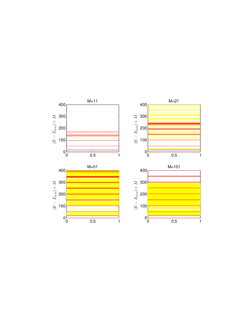
Figure 1: The energy levels of single trace states (red lines) and triple trace states (yellow lines) at $M=11$, M=21, M=51, and M=101 and the large $N$ limit. The blue dashed line is the threshold for multitrace states energy when $M=\infty$.

4 Energy spectrum at finite $N$

In this section, we show numerically how the energy levels change with respect to $N$ and the bit number $M$. We first introduce the methods to calculate the energy states of the system. We then analyze the result of the original Hamiltonian $H=H_{0}$, for which the $M=3$ case has been investigated in Ref. [20]. Next, we move to the Hamiltonians of the form $H=H_{0}+\xi\Delta H$ and investigate how the parameter $\xi$ affects the energy levels. Finally, we explore the Hamiltonians of the form $H=-H_{0}+\xi\Delta H$. For each case, we first analyze the change of energy levels with respect to $N$ when $M$ is fixed and then with respect to $M$ when $N$ is fixed.

4.1 $\mathcal{H}$ matrices

We have two methods to calculate the energy states of the system. Both methods involve the $\mathcal{H}$ matrix defined as

$$H\left|i\right\rangle=\sum_{j}\left|j\right\rangle\mathcal{H}_{ji},$$

where $\left|i\right\rangle$ and $\left|j\right\rangle$ are $M$-bit trace states. Note that, since the trace state basis is not orthonormal, $\mathcal{H}$ is not the Hamiltonian matrix and even not Hermitian.

The first method, used in Ref. [20], is to calculate the eigenvalues of the $\mathcal{H}$ from the equation

$$\mathcal{H}\left|E\right\rangle=E\left|E\right\rangle.$$ (26)

The relation between eigenvalues of $\mathcal{H}$ and of the Hamiltonian matrix is determined by the norm matrix, $G=\left\langle i|j\right\rangle$, as follows:

• If $G$ is positive definite, i.e., all its eigenvalues are positive, there is a one-to-one correspondence between the eigenvalues of $\mathcal{H}$ and the Hamiltonian. In this case, all the eigenstates of $\mathcal{H}$ are physical and have positive norm, which is defined as

  $$\left\langle E|E\right\rangle=\sum_{ij}v^{i*}\left\langle i|j\right\rangle v^{j}=v^{\dagger}Gv$$

  for an eigenstate $\left|E\right\rangle=\sum_{i}\left|i\right\rangle v^{i}$. Our numerical calculation shows that when $N\geq M$ the norm matrix $G$ is always positive definite.

• When $N$ is an integer and less than $M$, the norm matrix $G$ is positive semidefinite; i.e., some eigenvalues are zero, and the others are positive. In this case, only those eigenstates of $\mathcal{H}$ with positive norm correspond to energy states of the Hamiltonian, while those eigenstates of $\mathcal{H}$ with zero norm are unphysical.

• When $N$ is a noninteger and less than $M$, the norm matrix $G$ is indefinite; i.e., $G$ has both positive and negative eigenvalues. There is a subtlety in this case. The eigenstates of $\mathcal{H}$ can be of positive norm, of zero norm, and of negative norm. The negative norm eigenstates of $\mathcal{H}$ stem from their coupling to ghost states, the eigenstates of $G$ of which the eigenvalues are negative. The zero and negative norm eigenstates are still unphysical. But positive norm eigenstates cannot be simply taken as energy states anymore. A positive norm eigenstate is a physical energy state if it is orthogonal to every ghost state.

From the above statements, we should treat positive norm eigenstates of $\mathcal{H}$ physical when $N$ is large enough or a small integral. Moreover, the eigenvalues of $\mathcal{H}$ can be nonreal. This occurs for both positive-semidefinite and indefinite cases. For a nonreal eigenvalue of $\mathcal{H}$, the norm of its eigenstate must be zero, and its complex conjugate is also an eigenvalue of $\mathcal{H}$.

The second method is to solve a generalized eigenvalue problem,

$$\left(G\mathcal{H}\right)\left|E\right\rangle=EG\left|E\right\rangle.$$ (27)

This method is helpful for filtering unphysical states when $G$ is positive semidefinite. If $G$ is a full-rank matrix, this is a regular generalized eigenvalue problem. If $G$ is not a full-rank matrix, to solve the equation, we need to remove some rows and columns from $G$ and $G\mathcal{H}$. If the rank of $G$ is $r$, we can pick $r$ independent rows and columns from $G$ and $\left(G\mathcal{H}\right)$ to form two $r\times r$ matrices as

$$\tilde{G} = \left(\begin{array}[]{cccc}G_{i_{1}i_{1}}&G_{i_{1}i_{2}}&\cdots&G_{i_{1}i_{r}}\\ G_{i_{2}i_{2}}&G_{i_{2}i_{2}}&\cdots&G_{i_{2}i_{r}}\\ \vdots&\vdots&\vdots&\vdots\\ G_{i_{r}i_{1}}&G_{i_{r}i_{2}}&\cdots&G_{i_{r}i_{r}}\end{array}\right),$$

$$\widetilde{G\mathcal{H}} = \left(\begin{array}[]{cccc}\left(G\mathcal{H}\right)_{i_{1}i_{1}}&\left(G\mathcal{H}\right)_{i_{1}i_{2}}&\cdots&\left(G\mathcal{H}\right)_{i_{1}i_{r}}\\ \left(G\mathcal{H}\right)_{i_{2}i_{2}}&\left(G\mathcal{H}\right)_{i_{2}i_{2}}&\cdots&\left(G\mathcal{H}\right)_{i_{2}i_{r}}\\ \vdots&\vdots&\vdots&\vdots\\ \left(G\mathcal{H}\right)_{i_{r}i_{1}}&\left(G\mathcal{H}\right)_{i_{r}i_{2}}&\cdots&\left(G\mathcal{H}\right)_{i_{r}i_{r}}\end{array}\right).$$

Then, Eq. (27) becomes

$$\left(\widetilde{G\mathcal{H}}\right)\left|E\right\rangle=E\tilde{G}\left|E\right\rangle,$$

the eigenvalues and eigenstates of which are all physical.

The first method is used to investigate the change of eigenstates, including both physical and unphysical states, with respect to $N$ for fixed $M$, while the second one is for the change of physical energy levels with respect to $M$ for fixed $N$. For different values of $M$, we calculated the $\mathcal{H}$ and $G$ matrices, the entries of which are expressed in terms of $N$. Then we solve Eq. (26) or (27) to find their eigenstates. Since the number of trace states increases exponentially as $M$ increases, it is only feasible to perform the calculation for small $M$. The highest value of $M$ we study is 11, at which $\mathcal{H}$ and $G$ are $1473\times 1473$ matrices.

4.2 $H=H_{0}$

Let us first consider the case of odd $M$. Figures 2 to 6 show the lowest five eigenvalues of $\mathcal{H}$ as a function of $1/N$ for odd $M$ from 3 to 11. We use different line styles for different norm types: solid, dotted, and dash-dotted curves correspond to positive, negative, and zero norm eigenstates, respectively. Dash-dotted curves are actually associated with two complex eigenvalues which are conjugate to each other and hence represent only the real part of the eigenvalues. For higher $M$, the eigenvalues decline dramatically in higher $1/N$, which would squeeze the lower $1/N$ part into a small vertical size. To show more details in lower $1/N$, we split some plots into a lower $1/N$ part and a higher $1/N$ part, between which curves of the same color represent the same eigenstate. See Fig. 4 as an example.

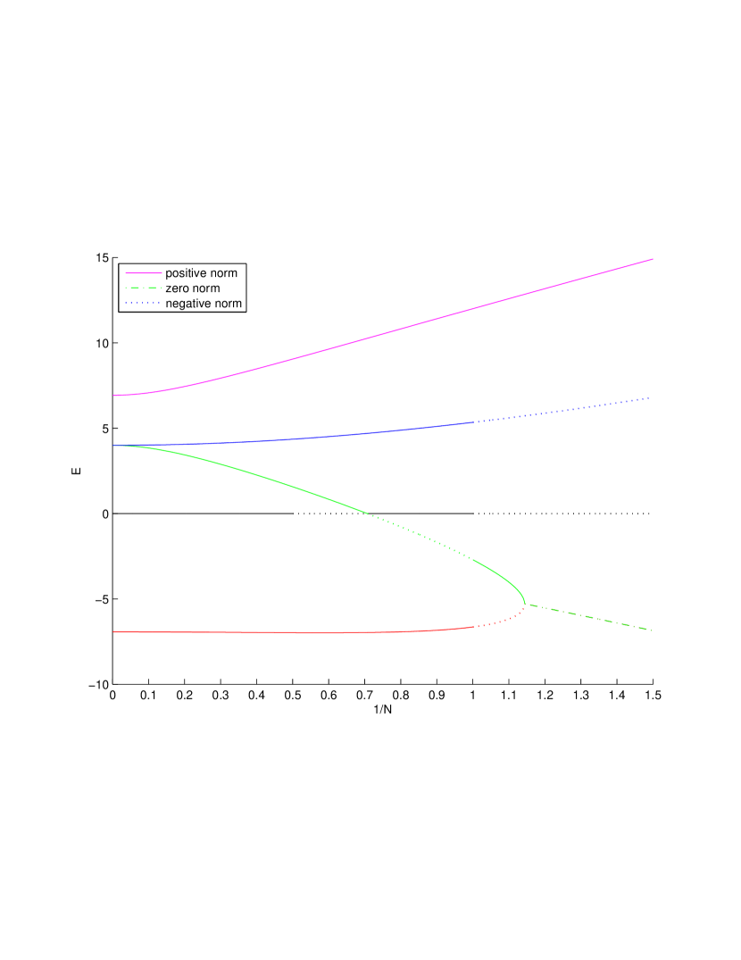
Figure 2: Lowest five energy states of the 3-bit system with Hamiltonian $H=H_{0}$.

From these figures, we see several features of the eigenstates of $\mathcal{H}$. At $N=\infty$, the ground states are nondegenerate, while the first excited states are nondegenerate for $M$ divisible by 3 and degenerate otherwise. This is consistent with the analytic discussion of the previous section. As $1/N$ increases, degeneracies are broken and the solid curves turn to dotted or dash-dotted curves, which implies the disappearance of physical states. If a physical state disappears at an integer value $N=n$, it also disappears at $N=n-1,\,n-2$, and etc. For convenience, we denote as $N_{M}^{*}$ the maximum value of $N$ where the first disappearance of the ground state occurs for bit number $M$. From the figures, we see that $N_{M}^{*}=\left(M-1\right)/2$ for $M\leq 11$. If it is true for all $M$, it follows that, for ground states surviving, $N$ must increase linearly as $M$ increases. The eigenvalues drop dramatically at large $1/N$, as the right parts of Figs. 4 to 6 show. But it does not imply the decrease of energy levels, since all these eigenstates are actually unphysical.

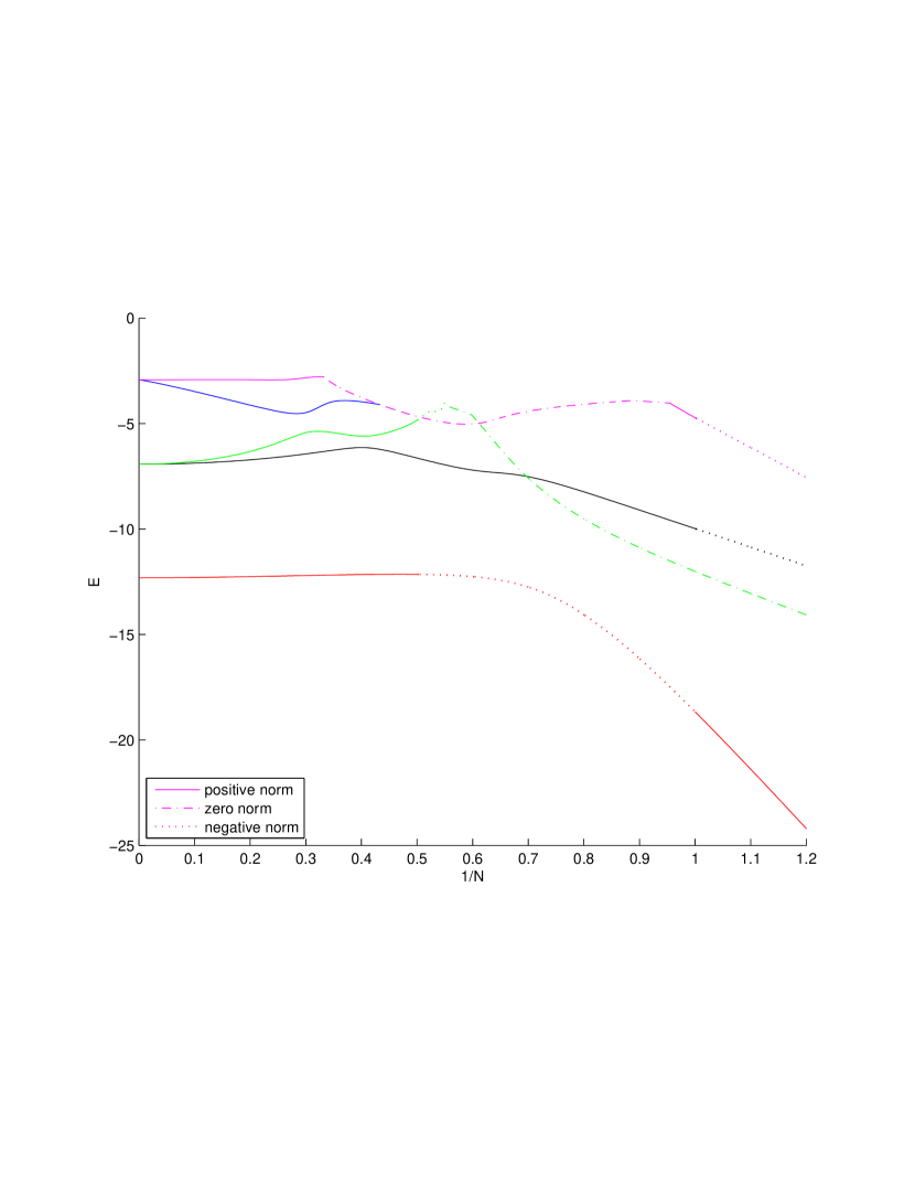
Figure 3: Lowest five eigenstates of $\mathcal{H}$ at $M=5$ for $H=H_{0}$.

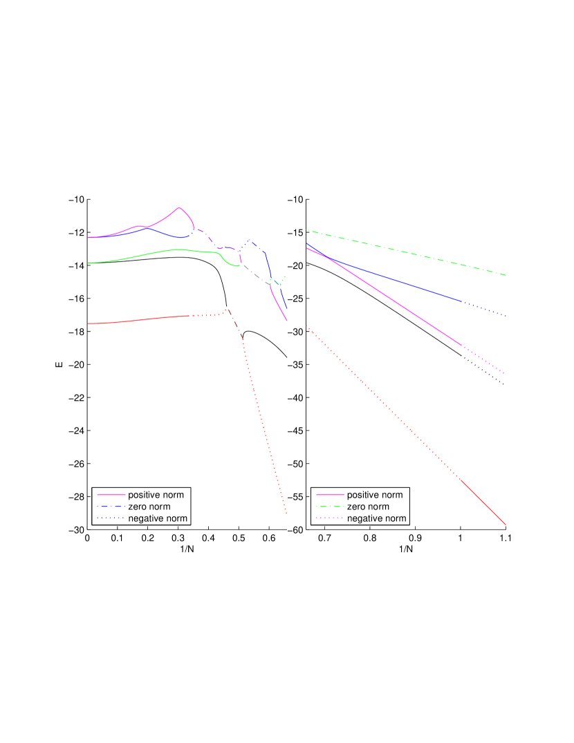
Figure 4: Lowest five eigenstates of $\mathcal{H}$ at $M=7$ for $H=H_{0}$.

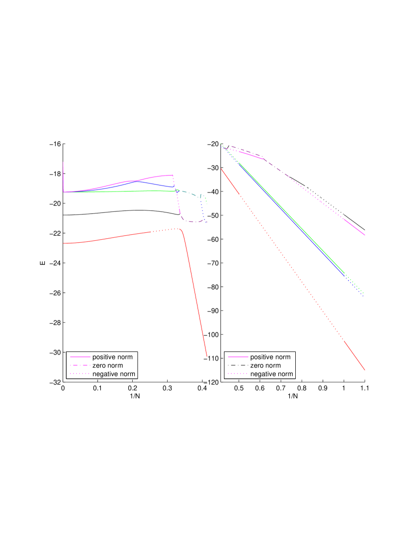
Figure 5: Lowest five eigenstates of $\mathcal{H}$ at $M=9$ for $H=H_{0}$.

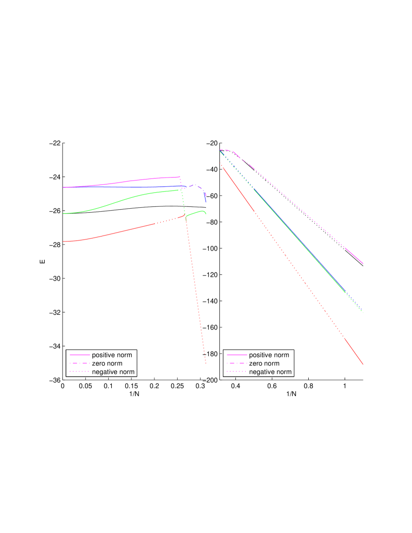
Figure 6: Lowest five eigenstates of $\mathcal{H}$ at $M=11$ for $H=H_{0}$.

For even $M$, we have similar plots as Fig. 7. At $N=\infty$, the lowest eigenstates are degenerate for $M=4$ and $8$ and nondegenerate for $M=6$ and 10. It is again consistent with our analysis in the previous section. The lowest states also disappear when $N$ is small. But unlike the odd $M$ case, there is no simple formula to determine $N_{M}^{*}$. The reason is that the lowest energy of $E\left(\eta_{i}\right)$ in (22) is excluded by the cyclic constraint (24).

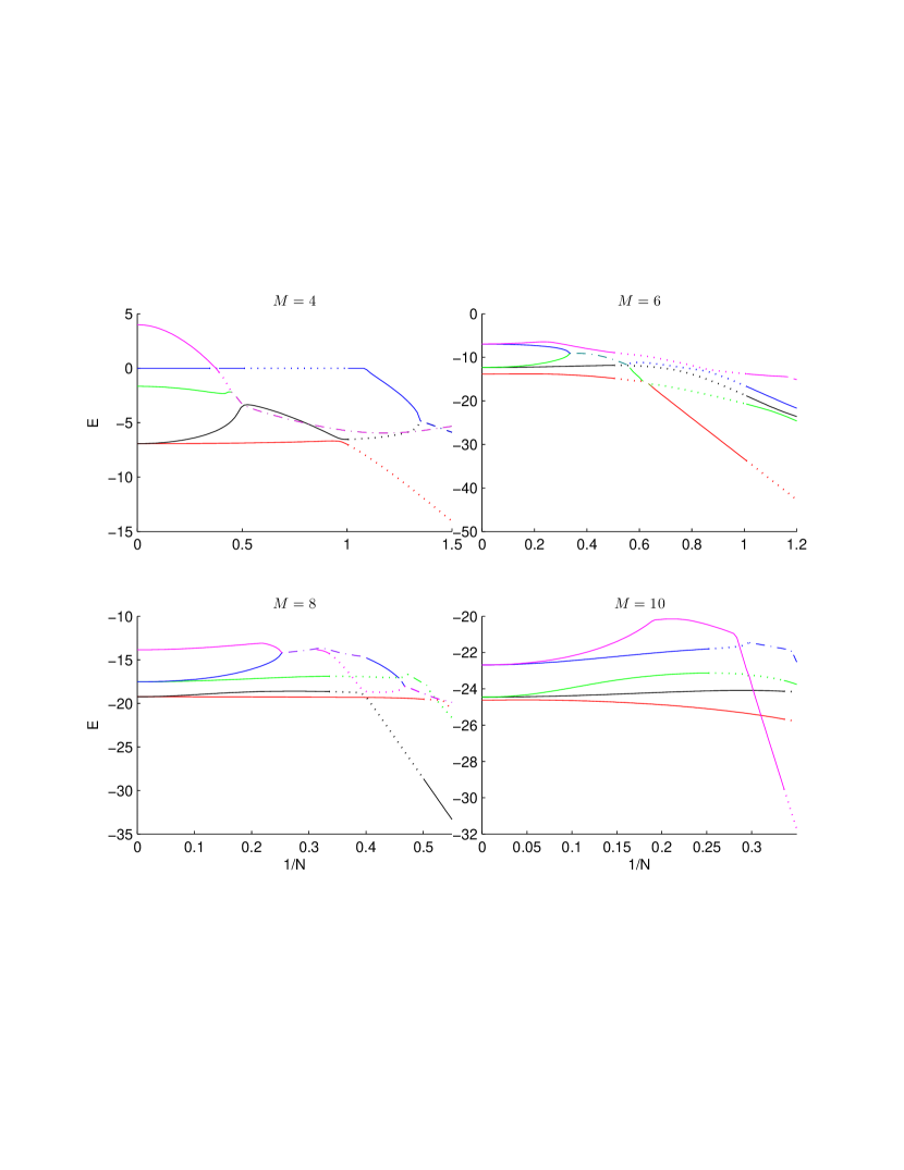
Figure 7: Lowest five eigenstates of $\mathcal{H}$ for $H=H_{0}$ at $M=4,6,8,10$

We now consider the physical ground energy as a function of $M$ when $N$ is fixed, shown as Fig. 8. The physical ground states have different trends at different values of $N$. For $N=1$, the physical ground state climbs significantly. This is consistent with analytical calculation, which shows the ground state is a quadratic function of $M$ when $N=1$. For $N=2$, the ground state only goes up slightly. When $N\geq 3$, it turns downward. For large $N$, the physical ground energy drops almost linearly with respect to $M$ at rate $-8/\pi$, as predicted by Eq. (25). This indicates the system becomes stringy when $N$ is large enough.

Figure 8: Change of physical ground states with respect to $M$ for fixed $N$. Only the ground energies at odd $M$ are sampled.

Fig. 9 shows how the excitation energy changes with respect to $M$ for fixed $N$. The vertical axis of Fig. 9 is $M\times\left(E_{1}-E_{0}\right)$, where $E_{1}-E_{0}$ is the gap between the first excited energy and lowest energy. For stringy behavior, $M\times\left(E_{1}-E_{0}\right)$ should be constant for large $M$. Though we only calculate up to $M=11$, we still see the trend that, for $N$ large enough, $M\times\left(E_{1}-E_{0}\right)$ is almost a constant between 15 and 20. As a reference, the analytic prediction of the gap at $N=\infty$ is $16\pi/3M$. That being said, there is no inconsistency between the numerical results and stringy behavior.

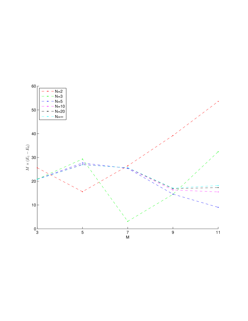
Figure 9: $\left(E_{1}-E_{0}\right)\times M$ as a function of $M$

4.3 Variations of $H$

In this subsection, we will analyze the energy levels of two variations of the Hamiltonian, $H=H_{0}+\xi\Delta H$ and $H=-H_{0}+\xi\Delta H$.

Figure 10 shows the eigenvalues of $\mathcal{H}$ as a function of $1/N$ when $M=3$ and the Hamiltonian is of the form $H=H_{0}+\xi\Delta H$. As $\xi$ increases, the disappearance point of the highest eigenstate moves in the small $N$ direction: for $\xi=-1$, it is at $N=2$; for $\xi=-0.6$, it is at $N=1$; when $\xi\geq-0.1$, the disappearance point occurs after $N<1/2$. The disappearance point of the ground state, $N_{3}^{*}$, moves in the opposite direction: for $-1\leq\xi\leq-0.1$, $N_{3}^{*}=1$; for $\xi=0.5$, $1<N_{3}^{*}<2$; for $\xi=3$, $N_{3}^{*}=2$.

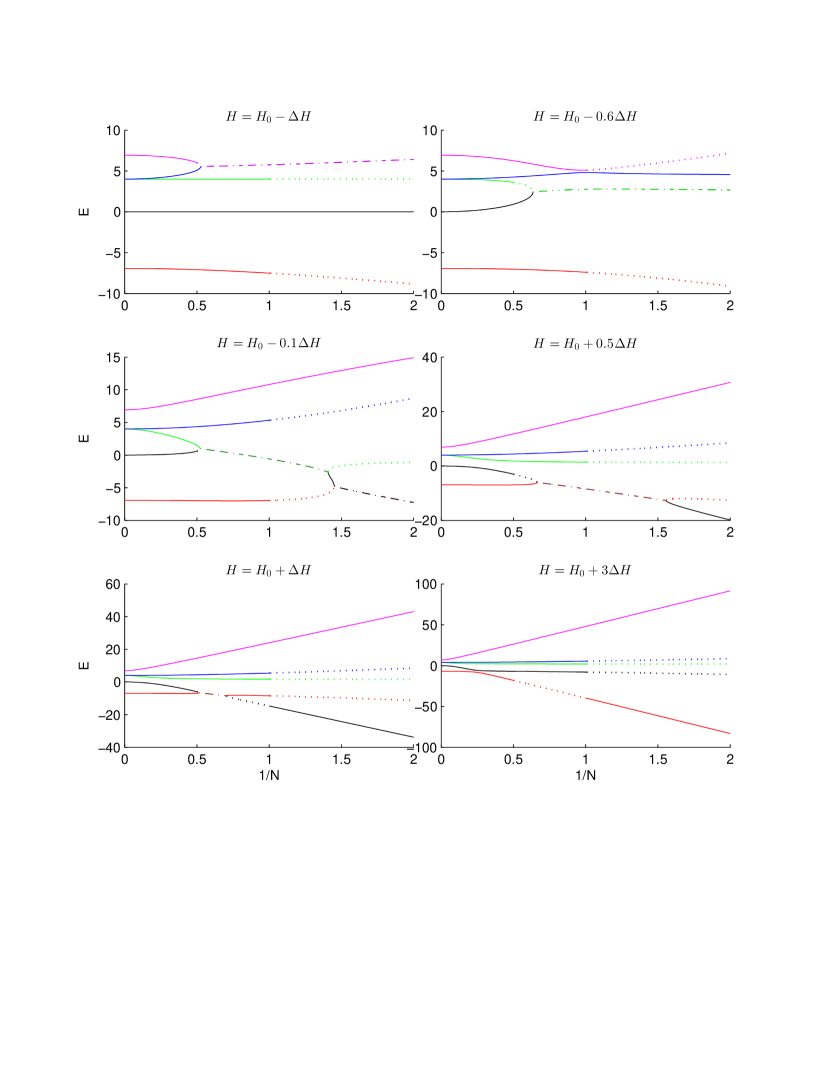
Figure 10: Eigenvalues of $\mathcal{H}$ matrices at $M=3$ for Hamiltonian $H=H_{0}+\xi\Delta H$, with $\xi=-1$, $-0.6$, $-0.1$, $0.5$, $1$, and $3$.

Since all eigenstates of $\mathcal{H}$ are physical when $N\geq M$, the largest value of $N_{M}^{*}$ is $M-1$. Particularly, for $M\leq 11$, we find $N_{M}^{*}=M-1$ can be achieved when $\xi\geq 2$. $N_{M}^{*}$ is minimal when $\xi=-1$, the lower bound of $\xi$ under the stabilization constraint. The $\xi=-1$ case is shown in Fig. 11. While $N_{M}^{*}=\left(M-1\right)/2$ still holds for $M=5$ and $7$, $N_{9}^{*}=2$ and $N_{11}^{*}=3$ spoil the pattern. We do not have results for $M>11$, but it seems that $M/N_{M}^{*}$ could be large for large $M$. If it is true, it means that the ground eigenstates could survive when $M$ is large and $N\ll M$.

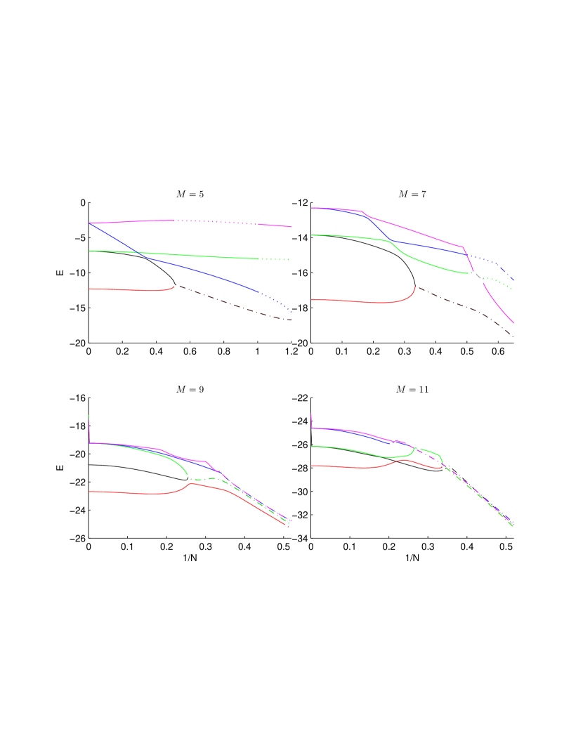
Figure 11: Lowest five eigenstates of $\mathcal{H}$ for $H=H_{0}-\Delta H$ at $M=5,7,9,11$

Figure 12 shows the change of physical ground energy with respect to $M$ for a fixed value of $N$. Note that only ground energies at odd $M$ are evaluated. The ground energies have different trends for $\xi<-1$, $\xi=-1$, and $\xi>-1$: when $\xi=-1$, the ground energies decrease almost linearly for all $N$; when $\xi<-1$, the ground energies decline faster than linearly, which implies the system is not stable; when $\xi>-1$, the ground energy first declines and then increases for small $N$, and it declines linearly for large $N$. It follows that the system has stringy behavior if $\xi\geq-1$ and $N$ is not too small.

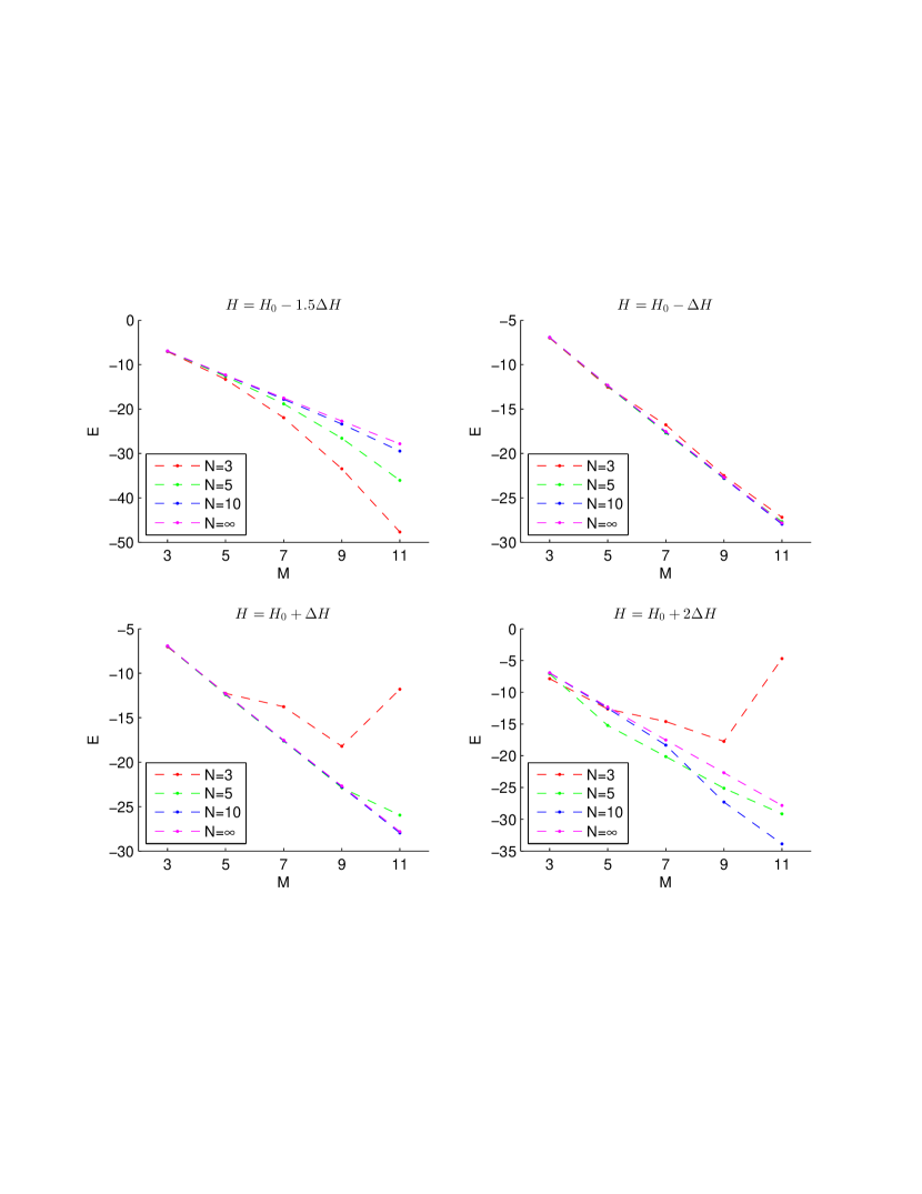
Figure 12: Change of physical ground energy with respect to $M$ at fixed $N$

For $H=-H_{0}+\xi\Delta H$, in the large $N$ limit, the maximum value of $E\left(\eta_{i}\right)$ in (22) is allowed for both odd and even $M$. Consequently, the ground eigenstates are nondegenerate for all $M$, as shown in Fig. 13 for $H=-H_{0}+1.5\Delta H$. From the figure, we see that $N_{M}^{*}=M-1$.

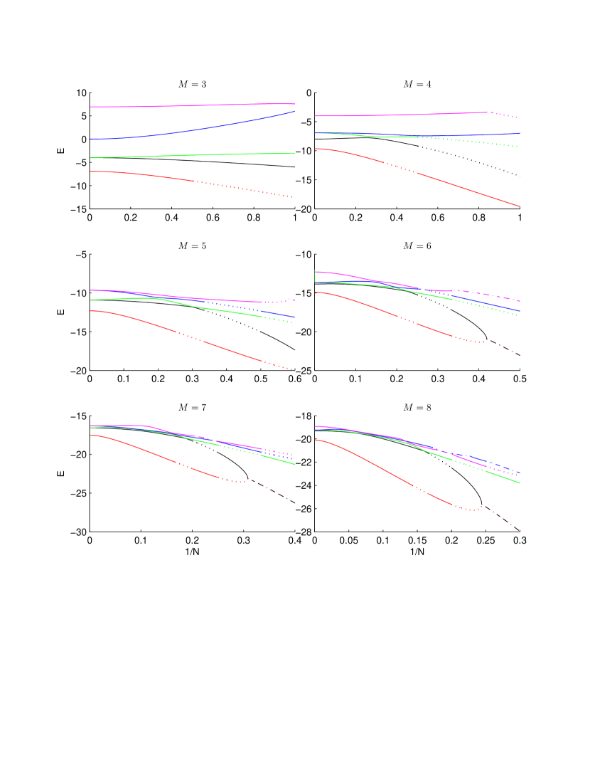
Figure 13: Eigenvalues of $\mathcal{H}$ for $H=-H_{0}+1.5\Delta H$. For each $M$, the ground state disappears at $N=M-1$.

$\xi$ has a similar impact on $N_{M}^{*}$ as the $H=H_{0}+\xi\Delta H$ case. Figure 14 plots the eigenstates of $\mathcal{H}$ for $\xi=1$, when $N_{M}^{*}$ is minimal. There is no simple pattern for $N_{M}^{*}$: for odd $M$, $N_{3}^{*}=2$, $N_{5}^{*}=2$, $N_{7}^{*}=3$, and $N_{9}^{*}=3$; for even $M$, $N_{4}^{*}=3$, $N_{6}^{*}=2$, $N_{8}=2$, and $N_{10}^{*}=3$. It seems to suggest that the ground eigenstate could survive when $M$ is large and $N\ll M$.

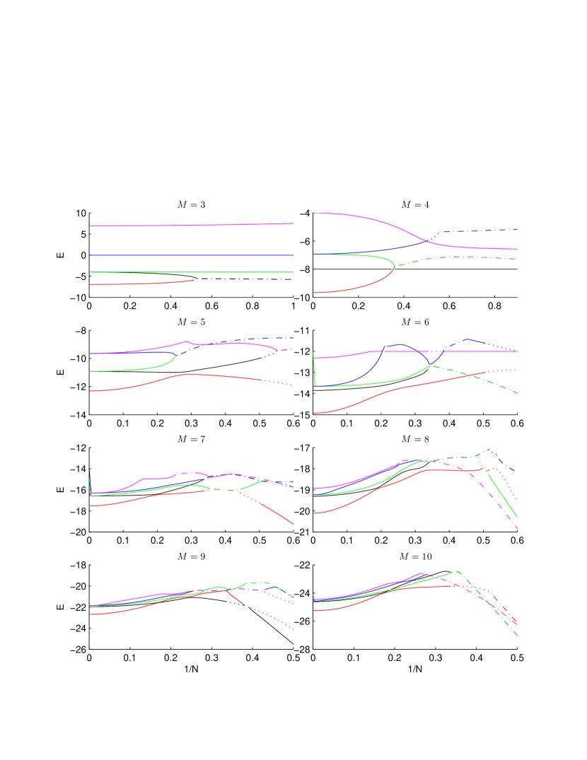
Figure 14: Eigenvalues of $\mathcal{H}$ for $H=-H_{0}+\Delta H$ and $3\leq M\leq 10$.

Figure 15 shows the change of physical ground energy with respect to $M$ at fixed $N$ for $H=-H_{0}+\xi\Delta H$. It is similar to the $H=H_{0}+\xi\Delta H$ case. When $\xi=0.5$, the system is not stable at finite $N$ as the curves decline faster than linearly. $\xi=1$ is the marginal case, in which all the physical ground energies drop almost linearly. When $\xi=1.5$ or $\xi=3$, the curves for small $N$ are zig-zag, and particularly, when $\xi=3$ and $N=3$, the trend is slightly upward. It implies that the system is stable for large $M$.

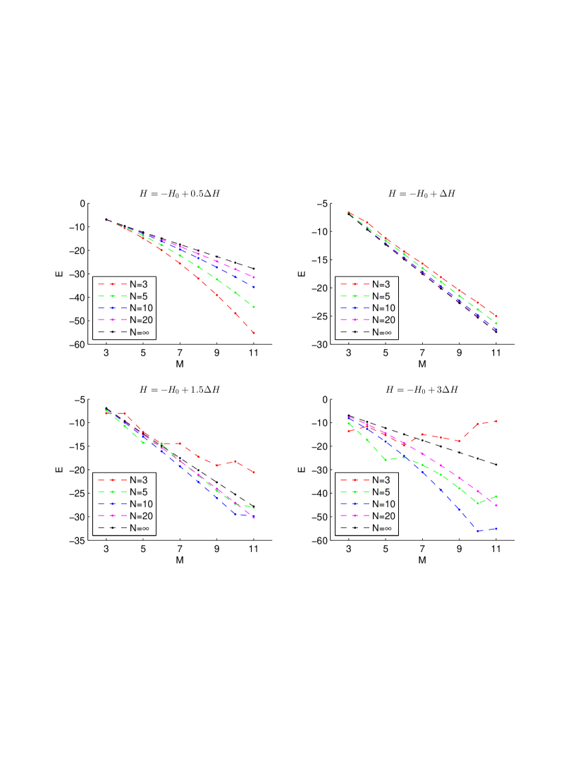
Figure 15: Physical ground energy of $-H_{0}+\xi\Delta H$ at $\xi=0.5,\,1,\,1.5,\,3$ and $N=3,\,5,\,10,\,20,\,\infty$.

5 Summary and conclusion

In this paper we have studied the string bit model with $s=1$, $d=0$. We studied possible forms of the supersymmetric Hamiltonian and their excitation energies in the large $N$ limit. We also performed a numerical study of energy levels at finite $N$ for Hamiltonians $H=\pm H_{0}+\xi\Delta H$, where, at $N=\infty$, $\Delta H$ vanishes and $H_{0}$ produces the Green-Schwarz Hamiltonian.

We showed that the supersymmetry plays a crucial role in the model. The general Hamiltonian is chosen to be a linear combination of eight single trace operators, which contain two consecutive creation operators followed by two annihilation operators. With the supersymmetry constraint, we reduce the number of parameters in the Hamiltonian to 3. Another interesting consequence of supersymmetry is that, after imposing the supersymmetry constraint on the Hamiltonian, the excitation energy becomes of order $M^{-1}$, which implies the energy spectrum of the model is continuous when $M$ is large.

In finite $N$, we numerically studied the energy spectrum of the model up to $M\leq 11$. There exists a maximal integer $N_{M}^{*}$ that when $N\leq N_{M}^{*}$ the would-be ground energy eigenstate of the $M$-bit system is unphysical. For $H=H_{0}$ and odd $M\leq 11$, the numerical computation shows $N_{M}^{*}=\left(M-1\right)/2$. If such a simple relation holds for all odd $M$, then, at large $M$, the surviving of ground state requires $N$ to be large as well. For $H=\pm H_{0}+\xi\Delta H$, $N_{M}^{*}$ increases (decreases) as $\xi$ increases (decreases). The maximum value of $N_{M}^{*}$ is $\left(M-1\right)$. The minimum of $N_{M}^{*}$ is achieved when $H=\pm H_{0}\mp\Delta H$ because of the stabilization constraint $\xi\geq\mp 1$. In the minimum cases, one find that $N_{M}^{*}$ is less than $\left(M-1\right)/2$ when $7<M\leq 11$ . If such a trend continues for $M>11$, it means that the ground energy state might be able to survive at very large $M$ and $M\gg N$.

For fixed finite $N$ and $H=\pm H_{0}+\xi\Delta H$, the system is stable only when $\xi\geq\mp 1$. The ground energy drops almost linearly with respect to $M$ when $\xi\geq\mp 1$ and faster than linearly when $\xi<\mp 1$. The numerical computation also reveals the excitation energy is roughly proportional to $M^{-1}$. While we do not have data for $M>11$, the trend is still evident. These properties indicate that the model has stringy behavior when $\xi\geq\mp 1$.

The numerical computation is performed up to $M=11$. The bottleneck is the calculation of norm matrices. Our algorithm has $\mathcal{O}\left(M!\right)$ time complexity for computing each entry of the matrix. It needs significant improvement for numerical computation of higher $M$. This is one of the issues we need to address in future research.

We can also extend our work in other directions. Our strategy can be applied to the model with $s>1,d=0$ or $d>0$ cases. We can also analytically calculate $1/N$ expansion of the model, in which some progress has been made by Ref. [23].

6 Acknowledgments

We thank Charles Thorn for his guidance on this work. This research was supported in part by the Department of Energy under Grant No. DE-SC0010296.

Appendix A Bosonic trace states

1. 1 bit

One bosonic state:

$$\left|1\right\rangle =\mathrm{Tr}\bar{a}\left|0\right\rangle$$

2. 2 bits

Two bosonic states:

$$\left|1\right\rangle =\mathrm{Tr}\bar{a}\bar{a}\left|0\right\rangle \left|2\right\rangle =\mathrm{Tr}\bar{a}\mathrm{Tr}\bar{a}\left|0\right\rangle$$

3. 3 bits

Five bosonic states:

$$\left|1\right\rangle =\mathrm{Tr}\bar{a}\bar{a}\bar{a}\left|0\right\rangle \left|2\right\rangle =\mathrm{Tr}\bar{a}\mathrm{Tr}\bar{a}\bar{a}\left|0\right\rangle \left|3\right\rangle =\mathrm{Tr}\bar{a}\mathrm{Tr}\bar{a}\mathrm{Tr}\bar{a}\left|0\right\rangle$$

$$\left|4\right\rangle =\mathrm{Tr}\bar{a}\bar{b}\bar{b}\left|0\right\rangle \left|5\right\rangle =\mathrm{Tr}\bar{b}\mathrm{Tr}\bar{a}\bar{b}\left|0\right\rangle$$

4. 4 bits

Ten bosonic states:

$$\left|1\right\rangle =\mathrm{Tr}\bar{a}\bar{a}\bar{a}\bar{a}\left|0\right\rangle \left|2\right\rangle =\mathrm{Tr}\bar{a}\mathrm{Tr}\bar{a}\bar{a}\bar{a}\left|0\right\rangle \left|3\right\rangle =\mathrm{Tr}\bar{a}\bar{a}\mathrm{Tr}\bar{a}\bar{a}\left|0\right\rangle$$

$$\left|4\right\rangle =\mathrm{Tr}\bar{a}\mathrm{Tr}\bar{a}\mathrm{Tr}\bar{a}\bar{a}\left|0\right\rangle \left|5\right\rangle =\mathrm{Tr}\bar{a}\mathrm{Tr}\bar{a}\mathrm{Tr}\bar{a}\mathrm{Tr}\bar{a}\left|0\right\rangle \left|6\right\rangle =\mathrm{Tr}\bar{a}\bar{a}\bar{b}\bar{b}\left|0\right\rangle$$

$$\left|7\right\rangle =\mathrm{Tr}\bar{a}\mathrm{Tr}\bar{a}\bar{b}\bar{b}\left|0\right\rangle \left|8\right\rangle =\mathrm{Tr}\bar{b}\mathrm{Tr}\bar{a}\bar{a}\bar{b}\left|0\right\rangle \left|9\right\rangle =\mathrm{Tr}\bar{a}\mathrm{Tr}\bar{b}\mathrm{Tr}\bar{a}\bar{b}\left|0\right\rangle$$

$$\left|10\right\rangle =\mathrm{Tr}\bar{b}\mathrm{Tr}\bar{b}\bar{b}\bar{b}\left|0\right\rangle$$

5. 5 bits

Twenty-one bosonic states:

$$\left|1\right\rangle =\mathrm{Tr}\bar{a}\bar{a}\bar{a}\bar{a}\bar{a}\left|0\right\rangle \left|2\right\rangle =\mathrm{Tr}\bar{a}\mathrm{Tr}\bar{a}\bar{a}\bar{a}\bar{a}\left|0\right\rangle \left|3\right\rangle =\mathrm{Tr}\bar{a}\bar{a}\mathrm{Tr}\bar{a}\bar{a}\bar{a}\left|0\right\rangle$$

$$\left|4\right\rangle =\mathrm{Tr}\bar{a}\mathrm{Tr}\bar{a}\mathrm{Tr}\bar{a}\bar{a}\bar{a}\left|0\right\rangle \left|5\right\rangle =\mathrm{Tr}\bar{a}\mathrm{Tr}\bar{a}\bar{a}\mathrm{Tr}\bar{a}\bar{a}\left|0\right\rangle \left|6\right\rangle =\mathrm{Tr}\bar{a}\mathrm{Tr}\bar{a}\mathrm{Tr}\bar{a}\mathrm{Tr}\bar{a}\bar{a}\left|0\right\rangle$$

$$\left|7\right\rangle =\mathrm{Tr}\bar{a}\mathrm{Tr}\bar{a}\mathrm{Tr}\bar{a}\mathrm{Tr}\bar{a}\mathrm{Tr}\bar{a}\left|0\right\rangle \left|8\right\rangle =\mathrm{Tr}\bar{a}\bar{a}\bar{a}\bar{b}\bar{b}\left|0\right\rangle \left|9\right\rangle =\mathrm{Tr}\bar{a}\bar{a}\bar{b}\bar{a}\bar{b}\left|0\right\rangle$$

$$\left|10\right\rangle =\mathrm{Tr}\bar{a}\mathrm{Tr}\bar{a}\bar{a}\bar{b}\bar{b}\left|0\right\rangle \left|11\right\rangle =\mathrm{Tr}\bar{b}\mathrm{Tr}\bar{a}\bar{a}\bar{a}\bar{b}\left|0\right\rangle \left|12\right\rangle =\mathrm{Tr}\bar{a}\bar{a}\mathrm{Tr}\bar{a}\bar{b}\bar{b}\left|0\right\rangle$$

$$\left|13\right\rangle =\mathrm{Tr}\bar{a}\bar{b}\mathrm{Tr}\bar{a}\bar{a}\bar{b}\left|0\right\rangle \left|14\right\rangle =\mathrm{Tr}\bar{a}\mathrm{Tr}\bar{a}\mathrm{Tr}\bar{a}\bar{b}\bar{b}\left|0\right\rangle \left|15\right\rangle =\mathrm{Tr}\bar{a}\mathrm{Tr}\bar{b}\mathrm{Tr}\bar{a}\bar{a}\bar{b}\left|0\right\rangle$$

$$\left|16\right\rangle =\mathrm{Tr}\bar{b}\mathrm{Tr}\bar{a}\bar{a}\mathrm{Tr}\bar{a}\bar{b}\left|0\right\rangle \left|17\right\rangle =\mathrm{Tr}\bar{a}\mathrm{Tr}\bar{a}\mathrm{Tr}\bar{b}\mathrm{Tr}\bar{a}\bar{b}\left|0\right\rangle \left|18\right\rangle =\mathrm{Tr}\bar{a}\bar{b}\bar{b}\bar{b}\bar{b}\left|0\right\rangle$$

$$\left|19\right\rangle =\mathrm{Tr}\bar{b}\mathrm{Tr}\bar{a}\bar{b}\bar{b}\bar{b}\left|0\right\rangle \left|20\right\rangle =\mathrm{Tr}\bar{a}\bar{b}\mathrm{Tr}\bar{b}\bar{b}\bar{b}\left|0\right\rangle \left|21\right\rangle =\mathrm{Tr}\bar{a}\mathrm{Tr}\bar{b}\mathrm{Tr}\bar{b}\bar{b}\bar{b}\left|0\right\rangle$$

6. 6 bits

Forty-four bosonic states:

$$\left|1\right\rangle =\mathrm{Tr}\bar{a}\bar{a}\bar{a}\bar{a}\bar{a}\bar{a}\left|0\right\rangle \left|2\right\rangle =\mathrm{Tr}\bar{a}\mathrm{Tr}\bar{a}\bar{a}\bar{a}\bar{a}\bar{a}\left|0\right\rangle \left|3\right\rangle =\mathrm{Tr}\bar{a}\bar{a}\mathrm{Tr}\bar{a}\bar{a}\bar{a}\bar{a}\left|0\right\rangle$$

$$\left|4\right\rangle =\mathrm{Tr}\bar{a}\bar{a}\bar{a}\mathrm{Tr}\bar{a}\bar{a}\bar{a}\left|0\right\rangle \left|5\right\rangle =\mathrm{Tr}\bar{a}\mathrm{Tr}\bar{a}\mathrm{Tr}\bar{a}\bar{a}\bar{a}\bar{a}\left|0\right\rangle \left|6\right\rangle =\mathrm{Tr}\bar{a}\mathrm{Tr}\bar{a}\bar{a}\mathrm{Tr}\bar{a}\bar{a}\bar{a}\left|0\right\rangle$$

$$\left|7\right\rangle =\mathrm{Tr}\bar{a}\bar{a}\mathrm{Tr}\bar{a}\bar{a}\mathrm{Tr}\bar{a}\bar{a}\left|0\right\rangle \left|8\right\rangle =\mathrm{Tr}\bar{a}\mathrm{Tr}\bar{a}\mathrm{Tr}\bar{a}\mathrm{Tr}\bar{a}\bar{a}\bar{a}\left|0\right\rangle \left|9\right\rangle =\mathrm{Tr}\bar{a}\mathrm{Tr}\bar{a}\mathrm{Tr}\bar{a}\bar{a}\mathrm{Tr}\bar{a}\bar{a}\left|0\right\rangle$$

$$\left|10\right\rangle =\mathrm{Tr}\bar{a}\mathrm{Tr}\bar{a}\mathrm{Tr}\bar{a}\mathrm{Tr}\bar{a}\mathrm{Tr}\bar{a}\bar{a}\left|0\right\rangle \left|11\right\rangle =\mathrm{Tr}\bar{a}\mathrm{Tr}\bar{a}\mathrm{Tr}\bar{a}\mathrm{Tr}\bar{a}\mathrm{Tr}\bar{a}\mathrm{Tr}\bar{a}\left|0\right\rangle \left|12\right\rangle =\mathrm{Tr}\bar{a}\bar{a}\bar{a}\bar{a}\bar{b}\bar{b}\left|0\right\rangle$$

$$\left|13\right\rangle =\mathrm{Tr}\bar{a}\bar{a}\bar{a}\bar{b}\bar{a}\bar{b}\left|0\right\rangle \left|14\right\rangle =\mathrm{Tr}\bar{a}\mathrm{Tr}\bar{a}\bar{a}\bar{a}\bar{b}\bar{b}\left|0\right\rangle \left|15\right\rangle =\mathrm{Tr}\bar{a}\mathrm{Tr}\bar{a}\bar{a}\bar{b}\bar{a}\bar{b}\left|0\right\rangle$$

$$\left|16\right\rangle =\mathrm{Tr}\bar{b}\mathrm{Tr}\bar{a}\bar{a}\bar{a}\bar{a}\bar{b}\left|0\right\rangle \left|17\right\rangle =\mathrm{Tr}\bar{a}\bar{a}\mathrm{Tr}\bar{a}\bar{a}\bar{b}\bar{b}\left|0\right\rangle \left|18\right\rangle =\mathrm{Tr}\bar{a}\bar{b}\mathrm{Tr}\bar{a}\bar{a}\bar{a}\bar{b}\left|0\right\rangle$$

$$\left|19\right\rangle =\mathrm{Tr}\bar{a}\bar{a}\bar{a}\mathrm{Tr}\bar{a}\bar{b}\bar{b}\left|0\right\rangle \left|20\right\rangle =\mathrm{Tr}\bar{a}\mathrm{Tr}\bar{a}\mathrm{Tr}\bar{a}\bar{a}\bar{b}\bar{b}\left|0\right\rangle \left|21\right\rangle =\mathrm{Tr}\bar{a}\mathrm{Tr}\bar{b}\mathrm{Tr}\bar{a}\bar{a}\bar{a}\bar{b}\left|0\right\rangle$$

$$\left|22\right\rangle =\mathrm{Tr}\bar{a}\mathrm{Tr}\bar{a}\bar{a}\mathrm{Tr}\bar{a}\bar{b}\bar{b}\left|0\right\rangle \left|23\right\rangle =\mathrm{Tr}\bar{a}\mathrm{Tr}\bar{a}\bar{b}\mathrm{Tr}\bar{a}\bar{a}\bar{b}\left|0\right\rangle \left|24\right\rangle =\mathrm{Tr}\bar{b}\mathrm{Tr}\bar{a}\bar{a}\mathrm{Tr}\bar{a}\bar{a}\bar{b}\left|0\right\rangle$$

$$\left|25\right\rangle =\mathrm{Tr}\bar{b}\mathrm{Tr}\bar{a}\bar{b}\mathrm{Tr}\bar{a}\bar{a}\bar{a}\left|0\right\rangle \left|26\right\rangle =\mathrm{Tr}\bar{a}\mathrm{Tr}\bar{a}\mathrm{Tr}\bar{a}\mathrm{Tr}\bar{a}\bar{b}\bar{b}\left|0\right\rangle \left|27\right\rangle =\mathrm{Tr}\bar{a}\mathrm{Tr}\bar{a}\mathrm{Tr}\bar{b}\mathrm{Tr}\bar{a}\bar{a}\bar{b}\left|0\right\rangle$$

$$\left|28\right\rangle =\mathrm{Tr}\bar{a}\mathrm{Tr}\bar{b}\mathrm{Tr}\bar{a}\bar{a}\mathrm{Tr}\bar{a}\bar{b}\left|0\right\rangle \left|29\right\rangle =\mathrm{Tr}\bar{a}\mathrm{Tr}\bar{a}\mathrm{Tr}\bar{a}\mathrm{Tr}\bar{b}\mathrm{Tr}\bar{a}\bar{b}\left|0\right\rangle \left|30\right\rangle =\mathrm{Tr}\bar{a}\bar{a}\bar{b}\bar{b}\bar{b}\bar{b}\left|0\right\rangle$$

$$\left|31\right\rangle =\mathrm{Tr}\bar{a}\bar{b}\bar{a}\bar{b}\bar{b}\bar{b}\left|0\right\rangle \left|32\right\rangle =\mathrm{Tr}\bar{a}\bar{b}\bar{b}\bar{a}\bar{b}\bar{b}\left|0\right\rangle \left|33\right\rangle =\mathrm{Tr}\bar{a}\mathrm{Tr}\bar{a}\bar{b}\bar{b}\bar{b}\bar{b}\left|0\right\rangle$$

$$\left|34\right\rangle =\mathrm{Tr}\bar{b}\mathrm{Tr}\bar{a}\bar{a}\bar{b}\bar{b}\bar{b}\left|0\right\rangle \left|35\right\rangle =\mathrm{Tr}\bar{b}\mathrm{Tr}\bar{a}\bar{b}\bar{a}\bar{b}\bar{b}\left|0\right\rangle \left|36\right\rangle =\mathrm{Tr}\bar{a}\bar{b}\mathrm{Tr}\bar{a}\bar{b}\bar{b}\bar{b}\left|0\right\rangle$$

$$\left|37\right\rangle =\mathrm{Tr}\bar{a}\bar{a}\bar{b}\mathrm{Tr}\bar{b}\bar{b}\bar{b}\left|0\right\rangle \left|38\right\rangle =\mathrm{Tr}\bar{a}\bar{b}\bar{b}\mathrm{Tr}\bar{a}\bar{b}\bar{b}\left|0\right\rangle \left|39\right\rangle =\mathrm{Tr}\bar{a}\mathrm{Tr}\bar{b}\mathrm{Tr}\bar{a}\bar{b}\bar{b}\bar{b}\left|0\right\rangle$$

$$\left|40\right\rangle =\mathrm{Tr}\bar{a}\mathrm{Tr}\bar{a}\bar{b}\mathrm{Tr}\bar{b}\bar{b}\bar{b}\left|0\right\rangle \left|41\right\rangle =\mathrm{Tr}\bar{b}\mathrm{Tr}\bar{a}\bar{a}\mathrm{Tr}\bar{b}\bar{b}\bar{b}\left|0\right\rangle \left|42\right\rangle =\mathrm{Tr}\bar{b}\mathrm{Tr}\bar{a}\bar{b}\mathrm{Tr}\bar{a}\bar{b}\bar{b}\left|0\right\rangle$$

$$\left|43\right\rangle =\mathrm{Tr}\bar{a}\mathrm{Tr}\bar{a}\mathrm{Tr}\bar{b}\mathrm{Tr}\bar{b}\bar{b}\bar{b}\left|0\right\rangle \left|44\right\rangle =\mathrm{Tr}\bar{b}\mathrm{Tr}\bar{b}\bar{b}\bar{b}\bar{b}\bar{b}\left|0\right\rangle$$

7. 7 bits

Eighty-nine bosonic states:

$$\left|1\right\rangle =\mathrm{Tr}\bar{a}\bar{a}\bar{a}\bar{a}\bar{a}\bar{a}\bar{a}\left|0\right\rangle \left|2\right\rangle =\mathrm{Tr}\bar{a}\mathrm{Tr}\bar{a}\bar{a}\bar{a}\bar{a}\bar{a}\bar{a}\left|0\right\rangle \left|3\right\rangle =\mathrm{Tr}\bar{a}\bar{a}\mathrm{Tr}\bar{a}\bar{a}\bar{a}\bar{a}\bar{a}\left|0\right\rangle$$

$$\left|4\right\rangle =\mathrm{Tr}\bar{a}\bar{a}\bar{a}\mathrm{Tr}\bar{a}\bar{a}\bar{a}\bar{a}\left|0\right\rangle \left|5\right\rangle =\mathrm{Tr}\bar{a}\mathrm{Tr}\bar{a}\mathrm{Tr}\bar{a}\bar{a}\bar{a}\bar{a}\bar{a}\left|0\right\rangle \left|6\right\rangle =\mathrm{Tr}\bar{a}\mathrm{Tr}\bar{a}\bar{a}\mathrm{Tr}\bar{a}\bar{a}\bar{a}\bar{a}\left|0\right\rangle$$

$$\left|7\right\rangle =\mathrm{Tr}\bar{a}\mathrm{Tr}\bar{a}\bar{a}\bar{a}\mathrm{Tr}\bar{a}\bar{a}\bar{a}\left|0\right\rangle \left|8\right\rangle =\mathrm{Tr}\bar{a}\bar{a}\mathrm{Tr}\bar{a}\bar{a}\mathrm{Tr}\bar{a}\bar{a}\bar{a}\left|0\right\rangle \left|9\right\rangle =\mathrm{Tr}\bar{a}\mathrm{Tr}\bar{a}\mathrm{Tr}\bar{a}\mathrm{Tr}\bar{a}\bar{a}\bar{a}\bar{a}\left|0\right\rangle$$

$$\left|10\right\rangle =\mathrm{Tr}\bar{a}\mathrm{Tr}\bar{a}\mathrm{Tr}\bar{a}\bar{a}\mathrm{Tr}\bar{a}\bar{a}\bar{a}\left|0\right\rangle \left|11\right\rangle =\mathrm{Tr}\bar{a}\mathrm{Tr}\bar{a}\bar{a}\mathrm{Tr}\bar{a}\bar{a}\mathrm{Tr}\bar{a}\bar{a}\left|0\right\rangle \left|12\right\rangle =\mathrm{Tr}\bar{a}\mathrm{Tr}\bar{a}\mathrm{Tr}\bar{a}\mathrm{Tr}\bar{a}\mathrm{Tr}\bar{a}\bar{a}\bar{a}\left|0\right\rangle$$

$$\left|13\right\rangle =\mathrm{Tr}\bar{a}\mathrm{Tr}\bar{a}\mathrm{Tr}\bar{a}\mathrm{Tr}\bar{a}\bar{a}\mathrm{Tr}\bar{a}\bar{a}\left|0\right\rangle \left|14\right\rangle =\mathrm{Tr}\bar{a}\mathrm{Tr}\bar{a}\mathrm{Tr}\bar{a}\mathrm{Tr}\bar{a}\mathrm{Tr}\bar{a}\mathrm{Tr}\bar{a}\bar{a}\left|0\right\rangle \left|15\right\rangle =\mathrm{Tr}\bar{a}\mathrm{Tr}\bar{a}\mathrm{Tr}\bar{a}\mathrm{Tr}\bar{a}\mathrm{Tr}\bar{a}\mathrm{Tr}\bar{a}\mathrm{Tr}\bar{a}\left|0\right\rangle$$

$$\left|16\right\rangle =\mathrm{Tr}\bar{a}\bar{a}\bar{a}\bar{a}\bar{a}\bar{b}\bar{b}\left|0\right\rangle \left|17\right\rangle =\mathrm{Tr}\bar{a}\bar{a}\bar{a}\bar{a}\bar{b}\bar{a}\bar{b}\left|0\right\rangle \left|18\right\rangle =\mathrm{Tr}\bar{a}\bar{a}\bar{a}\bar{b}\bar{a}\bar{a}\bar{b}\left|0\right\rangle$$

$$\left|19\right\rangle =\mathrm{Tr}\bar{a}\mathrm{Tr}\bar{a}\bar{a}\bar{a}\bar{a}\bar{b}\bar{b}\left|0\right\rangle \left|20\right\rangle =\mathrm{Tr}\bar{a}\mathrm{Tr}\bar{a}\bar{a}\bar{a}\bar{b}\bar{a}\bar{b}\left|0\right\rangle \left|21\right\rangle =\mathrm{Tr}\bar{b}\mathrm{Tr}\bar{a}\bar{a}\bar{a}\bar{a}\bar{a}\bar{b}\left|0\right\rangle$$

$$\left|22\right\rangle =\mathrm{Tr}\bar{a}\bar{a}\mathrm{Tr}\bar{a}\bar{a}\bar{a}\bar{b}\bar{b}\left|0\right\rangle \left|23\right\rangle =\mathrm{Tr}\bar{a}\bar{a}\mathrm{Tr}\bar{a}\bar{a}\bar{b}\bar{a}\bar{b}\left|0\right\rangle \left|24\right\rangle =\mathrm{Tr}\bar{a}\bar{b}\mathrm{Tr}\bar{a}\bar{a}\bar{a}\bar{a}\bar{b}\left|0\right\rangle$$

$$\left|25\right\rangle =\mathrm{Tr}\bar{a}\bar{a}\bar{a}\mathrm{Tr}\bar{a}\bar{a}\bar{b}\bar{b}\left|0\right\rangle \left|26\right\rangle =\mathrm{Tr}\bar{a}\bar{a}\bar{b}\mathrm{Tr}\bar{a}\bar{a}\bar{a}\bar{b}\left|0\right\rangle \left|27\right\rangle =\mathrm{Tr}\bar{a}\bar{b}\bar{b}\mathrm{Tr}\bar{a}\bar{a}\bar{a}\bar{a}\left|0\right\rangle$$

$$\left|28\right\rangle =\mathrm{Tr}\bar{a}\mathrm{Tr}\bar{a}\mathrm{Tr}\bar{a}\bar{a}\bar{a}\bar{b}\bar{b}\left|0\right\rangle \left|29\right\rangle =\mathrm{Tr}\bar{a}\mathrm{Tr}\bar{a}\mathrm{Tr}\bar{a}\bar{a}\bar{b}\bar{a}\bar{b}\left|0\right\rangle \left|30\right\rangle =\mathrm{Tr}\bar{a}\mathrm{Tr}\bar{b}\mathrm{Tr}\bar{a}\bar{a}\bar{a}\bar{a}\bar{b}\left|0\right\rangle$$

$$\left|31\right\rangle =\mathrm{Tr}\bar{a}\mathrm{Tr}\bar{a}\bar{a}\mathrm{Tr}\bar{a}\bar{a}\bar{b}\bar{b}\left|0\right\rangle \left|32\right\rangle =\mathrm{Tr}\bar{a}\mathrm{Tr}\bar{a}\bar{b}\mathrm{Tr}\bar{a}\bar{a}\bar{a}\bar{b}\left|0\right\rangle \left|33\right\rangle =\mathrm{Tr}\bar{a}\mathrm{Tr}\bar{a}\bar{a}\bar{a}\mathrm{Tr}\bar{a}\bar{b}\bar{b}\left|0\right\rangle$$

$$\left|34\right\rangle =\mathrm{Tr}\bar{b}\mathrm{Tr}\bar{a}\bar{a}\mathrm{Tr}\bar{a}\bar{a}\bar{a}\bar{b}\left|0\right\rangle \left|35\right\rangle =\mathrm{Tr}\bar{b}\mathrm{Tr}\bar{a}\bar{b}\mathrm{Tr}\bar{a}\bar{a}\bar{a}\bar{a}\left|0\right\rangle \left|36\right\rangle =\mathrm{Tr}\bar{b}\mathrm{Tr}\bar{a}\bar{a}\bar{a}\mathrm{Tr}\bar{a}\bar{a}\bar{b}\left|0\right\rangle$$

$$\left|37\right\rangle =\mathrm{Tr}\bar{a}\bar{a}\mathrm{Tr}\bar{a}\bar{a}\mathrm{Tr}\bar{a}\bar{b}\bar{b}\left|0\right\rangle \left|38\right\rangle =\mathrm{Tr}\bar{a}\bar{a}\mathrm{Tr}\bar{a}\bar{b}\mathrm{Tr}\bar{a}\bar{a}\bar{b}\left|0\right\rangle \left|39\right\rangle =\mathrm{Tr}\bar{a}\mathrm{Tr}\bar{a}\mathrm{Tr}\bar{a}\mathrm{Tr}\bar{a}\bar{a}\bar{b}\bar{b}\left|0\right\rangle$$

$$\left|40\right\rangle =\mathrm{Tr}\bar{a}\mathrm{Tr}\bar{a}\mathrm{Tr}\bar{b}\mathrm{Tr}\bar{a}\bar{a}\bar{a}\bar{b}\left|0\right\rangle \left|41\right\rangle =\mathrm{Tr}\bar{a}\mathrm{Tr}\bar{a}\mathrm{Tr}\bar{a}\bar{a}\mathrm{Tr}\bar{a}\bar{b}\bar{b}\left|0\right\rangle \left|42\right\rangle =\mathrm{Tr}\bar{a}\mathrm{Tr}\bar{a}\mathrm{Tr}\bar{a}\bar{b}\mathrm{Tr}\bar{a}\bar{a}\bar{b}\left|0\right\rangle$$

$$\left|43\right\rangle =\mathrm{Tr}\bar{a}\mathrm{Tr}\bar{b}\mathrm{Tr}\bar{a}\bar{a}\mathrm{Tr}\bar{a}\bar{a}\bar{b}\left|0\right\rangle \left|44\right\rangle =\mathrm{Tr}\bar{a}\mathrm{Tr}\bar{b}\mathrm{Tr}\bar{a}\bar{b}\mathrm{Tr}\bar{a}\bar{a}\bar{a}\left|0\right\rangle \left|45\right\rangle =\mathrm{Tr}\bar{b}\mathrm{Tr}\bar{a}\bar{a}\mathrm{Tr}\bar{a}\bar{a}\mathrm{Tr}\bar{a}\bar{b}\left|0\right\rangle$$

$$\left|46\right\rangle =\mathrm{Tr}\bar{a}\mathrm{Tr}\bar{a}\mathrm{Tr}\bar{a}\mathrm{Tr}\bar{a}\mathrm{Tr}\bar{a}\bar{b}\bar{b}\left|0\right\rangle \left|47\right\rangle =\mathrm{Tr}\bar{a}\mathrm{Tr}\bar{a}\mathrm{Tr}\bar{a}\mathrm{Tr}\bar{b}\mathrm{Tr}\bar{a}\bar{a}\bar{b}\left|0\right\rangle \left|48\right\rangle =\mathrm{Tr}\bar{a}\mathrm{Tr}\bar{a}\mathrm{Tr}\bar{b}\mathrm{Tr}\bar{a}\bar{a}\mathrm{Tr}\bar{a}\bar{b}\left|0\right\rangle$$

$$\left|49\right\rangle =\mathrm{Tr}\bar{a}\mathrm{Tr}\bar{a}\mathrm{Tr}\bar{a}\mathrm{Tr}\bar{a}\mathrm{Tr}\bar{b}\mathrm{Tr}\bar{a}\bar{b}\left|0\right\rangle \left|50\right\rangle =\mathrm{Tr}\bar{a}\bar{a}\bar{a}\bar{b}\bar{b}\bar{b}\bar{b}\left|0\right\rangle \left|51\right\rangle =\mathrm{Tr}\bar{a}\bar{a}\bar{b}\bar{a}\bar{b}\bar{b}\bar{b}\left|0\right\rangle$$

$$\left|52\right\rangle =\mathrm{Tr}\bar{a}\bar{a}\bar{b}\bar{b}\bar{a}\bar{b}\bar{b}\left|0\right\rangle \left|53\right\rangle =\mathrm{Tr}\bar{a}\bar{a}\bar{b}\bar{b}\bar{b}\bar{a}\bar{b}\left|0\right\rangle \left|54\right\rangle =\mathrm{Tr}\bar{a}\bar{b}\bar{a}\bar{b}\bar{a}\bar{b}\bar{b}\left|0\right\rangle$$

$$\left|55\right\rangle =\mathrm{Tr}\bar{a}\mathrm{Tr}\bar{a}\bar{a}\bar{b}\bar{b}\bar{b}\bar{b}\left|0\right\rangle \left|56\right\rangle =\mathrm{Tr}\bar{a}\mathrm{Tr}\bar{a}\bar{b}\bar{a}\bar{b}\bar{b}\bar{b}\left|0\right\rangle \left|57\right\rangle =\mathrm{Tr}\bar{a}\mathrm{Tr}\bar{a}\bar{b}\bar{b}\bar{a}\bar{b}\bar{b}\left|0\right\rangle$$

$$\left|58\right\rangle =\mathrm{Tr}\bar{b}\mathrm{Tr}\bar{a}\bar{a}\bar{a}\bar{b}\bar{b}\bar{b}\left|0\right\rangle \left|59\right\rangle =\mathrm{Tr}\bar{b}\mathrm{Tr}\bar{a}\bar{a}\bar{b}\bar{a}\bar{b}\bar{b}\left|0\right\rangle \left|60\right\rangle =\mathrm{Tr}\bar{b}\mathrm{Tr}\bar{a}\bar{a}\bar{b}\bar{b}\bar{a}\bar{b}\left|0\right\rangle$$

$$\left|61\right\rangle =\mathrm{Tr}\bar{b}\mathrm{Tr}\bar{a}\bar{b}\bar{a}\bar{b}\bar{a}\bar{b}\left|0\right\rangle \left|62\right\rangle =\mathrm{Tr}\bar{a}\bar{a}\mathrm{Tr}\bar{a}\bar{b}\bar{b}\bar{b}\bar{b}\left|0\right\rangle \left|63\right\rangle =\mathrm{Tr}\bar{a}\bar{b}\mathrm{Tr}\bar{a}\bar{a}\bar{b}\bar{b}\bar{b}\left|0\right\rangle$$

$$\left|64\right\rangle =\mathrm{Tr}\bar{a}\bar{b}\mathrm{Tr}\bar{a}\bar{b}\bar{a}\bar{b}\bar{b}\left|0\right\rangle \left|65\right\rangle =\mathrm{Tr}\bar{a}\bar{a}\bar{b}\mathrm{Tr}\bar{a}\bar{b}\bar{b}\bar{b}\left|0\right\rangle \left|66\right\rangle =\mathrm{Tr}\bar{a}\bar{b}\bar{b}\mathrm{Tr}\bar{a}\bar{a}\bar{b}\bar{b}\left|0\right\rangle$$

$$\left|67\right\rangle =\mathrm{Tr}\bar{b}\bar{b}\bar{b}\mathrm{Tr}\bar{a}\bar{a}\bar{a}\bar{b}\left|0\right\rangle \left|68\right\rangle =\mathrm{Tr}\bar{a}\mathrm{Tr}\bar{a}\mathrm{Tr}\bar{a}\bar{b}\bar{b}\bar{b}\bar{b}\left|0\right\rangle \left|69\right\rangle =\mathrm{Tr}\bar{a}\mathrm{Tr}\bar{b}\mathrm{Tr}\bar{a}\bar{a}\bar{b}\bar{b}\bar{b}\left|0\right\rangle$$

$$\left|70\right\rangle =\mathrm{Tr}\bar{a}\mathrm{Tr}\bar{b}\mathrm{Tr}\bar{a}\bar{b}\bar{a}\bar{b}\bar{b}\left|0\right\rangle \left|71\right\rangle =\mathrm{Tr}\bar{a}\mathrm{Tr}\bar{a}\bar{b}\mathrm{Tr}\bar{a}\bar{b}\bar{b}\bar{b}\left|0\right\rangle \left|72\right\rangle =\mathrm{Tr}\bar{a}\mathrm{Tr}\bar{a}\bar{a}\bar{b}\mathrm{Tr}\bar{b}\bar{b}\bar{b}\left|0\right\rangle$$

$$\left|73\right\rangle =\mathrm{Tr}\bar{a}\mathrm{Tr}\bar{a}\bar{b}\bar{b}\mathrm{Tr}\bar{a}\bar{b}\bar{b}\left|0\right\rangle \left|74\right\rangle =\mathrm{Tr}\bar{b}\mathrm{Tr}\bar{a}\bar{a}\mathrm{Tr}\bar{a}\bar{b}\bar{b}\bar{b}\left|0\right\rangle \left|75\right\rangle =\mathrm{Tr}\bar{b}\mathrm{Tr}\bar{a}\bar{b}\mathrm{Tr}\bar{a}\bar{a}\bar{b}\bar{b}\left|0\right\rangle$$

$$\left|76\right\rangle =\mathrm{Tr}\bar{b}\mathrm{Tr}\bar{a}\bar{a}\bar{a}\mathrm{Tr}\bar{b}\bar{b}\bar{b}\left|0\right\rangle \left|77\right\rangle =\mathrm{Tr}\bar{b}\mathrm{Tr}\bar{a}\bar{a}\bar{b}\mathrm{Tr}\bar{a}\bar{b}\bar{b}\left|0\right\rangle \left|78\right\rangle =\mathrm{Tr}\bar{a}\bar{a}\mathrm{Tr}\bar{a}\bar{b}\mathrm{Tr}\bar{b}\bar{b}\bar{b}\left|0\right\rangle$$

$$\left|79\right\rangle =\mathrm{Tr}\bar{a}\mathrm{Tr}\bar{a}\mathrm{Tr}\bar{b}\mathrm{Tr}\bar{a}\bar{b}\bar{b}\bar{b}\left|0\right\rangle \left|80\right\rangle =\mathrm{Tr}\bar{a}\mathrm{Tr}\bar{a}\mathrm{Tr}\bar{a}\bar{b}\mathrm{Tr}\bar{b}\bar{b}\bar{b}\left|0\right\rangle \left|81\right\rangle =\mathrm{Tr}\bar{a}\mathrm{Tr}\bar{b}\mathrm{Tr}\bar{a}\bar{a}\mathrm{Tr}\bar{b}\bar{b}\bar{b}\left|0\right\rangle$$

$$\left|82\right\rangle =\mathrm{Tr}\bar{a}\mathrm{Tr}\bar{b}\mathrm{Tr}\bar{a}\bar{b}\mathrm{Tr}\bar{a}\bar{b}\bar{b}\left|0\right\rangle \left|83\right\rangle =\mathrm{Tr}\bar{a}\mathrm{Tr}\bar{a}\mathrm{Tr}\bar{a}\mathrm{Tr}\bar{b}\mathrm{Tr}\bar{b}\bar{b}\bar{b}\left|0\right\rangle \left|84\right\rangle =\mathrm{Tr}\bar{a}\bar{b}\bar{b}\bar{b}\bar{b}\bar{b}\bar{b}\left|0\right\rangle$$

$$\left|85\right\rangle =\mathrm{Tr}\bar{b}\mathrm{Tr}\bar{a}\bar{b}\bar{b}\bar{b}\bar{b}\bar{b}\left|0\right\rangle \left|86\right\rangle =\mathrm{Tr}\bar{a}\bar{b}\mathrm{Tr}\bar{b}\bar{b}\bar{b}\bar{b}\bar{b}\left|0\right\rangle \left|87\right\rangle =\mathrm{Tr}\bar{b}\bar{b}\bar{b}\mathrm{Tr}\bar{a}\bar{b}\bar{b}\bar{b}\left|0\right\rangle$$

$$\left|88\right\rangle =\mathrm{Tr}\bar{a}\mathrm{Tr}\bar{b}\mathrm{Tr}\bar{b}\bar{b}\bar{b}\bar{b}\bar{b}\left|0\right\rangle \left|89\right\rangle =\mathrm{Tr}\bar{b}\mathrm{Tr}\bar{a}\bar{b}\bar{b}\mathrm{Tr}\bar{b}\bar{b}\bar{b}\left|0\right\rangle$$

Appendix B Counting problems on trace states

How many trace states are there for a fixed bit number $M$? In this Appendix, we will first count the single trace states and then the trace states which includes both single and multiple trace states.

1. Counting single trace states

There are $2^{M}$ combinations of an $M$-bit string consisting of $\bar{a},\bar{b}$. By the property of trace, a trace state is equivalent to its cyclic permutations. For example, $\operatorname{Tr}\bar{b}\bar{a}$ and $\operatorname{Tr}\bar{a}\bar{b}$ are equivalent states, and so are $\operatorname{Tr}\bar{b}\bar{a}\bar{a}\bar{b}$ and $\operatorname{Tr}\bar{a}\bar{a}\bar{b}\bar{b}$. Actually, the latter case differs by a negative sign,

$$\operatorname{Tr}\bar{a}\bar{a}\bar{b}\bar{b}=-\operatorname{Tr}\bar{b}\bar{a}\bar{a}\bar{b}.$$

The rule is that each swap of two $\bar{b}$ introduces a minus sign. It follows that some trace states are vanishing, for example, $\operatorname{Tr}\bar{b}\bar{b}=-\operatorname{Tr}\bar{b}\bar{b}=0.$

To count the single trace states, we need the following definition and theorem [24].

Definition.

Given a group $G$ acting on a set $X$, the orbit of $x\in X$ is the set $Gx=\left\{g\cdot x|g\in G\right\}$. The set of orbits is denoted by $X/G$.

In our case, the cyclic group $C_{M}$ is the group $G$. $X$ is the $2^{M}$ combinations of $M$-bit operators, and $x$ corresponds to one particular combination. $X/G$ is the set of different combinations under the action of the cyclic group.

Theorem.

(Burnside’s counting theorem). —If $G$ is a finite group acting on a finite set $X$, then

$$\left|X/G\right|=\frac{1}{\left|G\right|}\sum_{g\in G}\left|\mathrm{Fix}\left(g\right)\right|,$$

where $\mathrm{Fix}\left(g\right)$ is the set of $x$ that is invariant under action of $g$, i.e.,

$$\mathrm{Fix}\left(g\right)=\left\{x\in X|g\cdot x=x\right\}.$$

To find the number of states, we need to find $\left|\mathrm{Fix}\left(g\right)\right|$ for each group member.

We first consider the odd $M$ case. Let $c_{k}\in C_{M},\,k=1,2,\cdots M$, be the group member that shifts $k$ operators from the tail of the trace to the beginning. The identity of the group is $e=c_{M}$. Let $\left(M,k\right)$ denote the greatest common divisor of $M$ and $k$. For group member $c_{k}$, we equally partition the $M$ bits into $M/\left(M,k\right)$ consecutive parts: the first part starts from bit 1 to bit $\left(M,k\right)$, the second part starts from bit $\left(M,k\right)+1$ to bit $2\left(M,k\right)$, etc. Under the action of $c_{k}$, the $i$th part transfers as

$$i\mathrm{th}\text{ part}\to\left(i+\frac{k}{\left(M,k\right)}\right)\mathrm{\text{th part}}.$$

The trace is invariant under $c_{k}$ if and only if all the parts are identical to each other. For bosonic trace states, each part need to bosonic, from which it follows that

$$\left|\mathrm{Fix}\left(c_{k}\right)\right|=\sum_{\text{even }i}\binom{\left(M,k\right)}{i}=\frac{1}{2}2^{\left(M,k\right)}.$$ (B.1)

Similarly, for fermionic single trace states, each part needs to be fermionic,

$$\left|\mathrm{Fix}\left(c_{k}\right)\right|=\sum_{\text{odd }i}\binom{\left(M,k\right)}{i}=\frac{1}{2}2^{\left(M,k\right)},$$ (B.2)

which implies there is the same number of bosonic and fermionic single trace states for odd $M$. By Burnside’s theorem, this number is given by

$$S_{M}=\frac{1}{2M}\sum_{k=1}^{M}2^{\left(M,k\right)}.$$ (B.3)

For even $M$, let us first consider the fermionic states. For a group member $c_{k}$, $\left|\mathrm{Fix}\left(c_{k}\right)\right|=0$ if $M/\left(M,k\right)$ is even. The reason is that an odd number of $\bar{b}$ cannot be equally partitioned into even parts. Therefore, only odd $M/\left(M,k\right)$ contributes to $\left|\mathrm{Fix}\left(c_{k}\right)\right|$, which is still given by (B.2). And Eq. (B.3) becomes

$$S_{M}=\frac{1}{2M}\sum_{M/\left(M,k\right)\text{ is odd}}2^{\left(M,k\right)}.$$ (B.4)

Let $i=M/\left(M,k\right)$; Eq. (B.4) can be written as

$$S_{M}=\frac{1}{2M}\sum_{\mathrm{odd}\,i,i|M}\varphi\left(i\right)2^{\frac{M}{i}},$$ (B.5)

where $\varphi\left(i\right)$ is the Euler totient function and $i|M$ means $M$ is divisible by $i$. We see that Eq. (B.3) can also be written as Eqs. (B.4) and (B.5).

For bosonic states, because there exist vanishing states, like $\operatorname{Tr}\bar{a}\bar{b}\bar{a}\bar{b}=-\operatorname{Tr}\bar{a}\bar{b}\bar{a}\bar{b}=0$, the number of bosonic states equals the number of even-$\bar{b}$ state minus the number of vanishing states. Consider the number of even-$\bar{b}$-states, which is denoted as $B_{M}$ for convenience. For a group member $c_{k}$, we partition $M$ bits equally into $M/\left(M,k\right)$ consecutive parts with each part $\left(M,k\right)$ bits: if $M/\left(M,k\right)$ is odd, we need even number of $\bar{b}$ in each part; if $M/\left(M,k\right)$ is even, there can be any number of $\bar{b}$ in each part, from which it follows that

$$B_{M} = \frac{1}{M}\left(\sum_{M/\left(M,k\right)\text{ is odd}}2^{\left(M,k\right)-1}+\sum_{M/\left(M,k\right)\text{ is even}}2^{\left(M,k\right)}\right)$$ (B.6)

$$= \frac{1}{2M}\left(\sum_{\mathrm{odd}\,i,i|M}\varphi\left(i\right)2^{\frac{M}{i}}+2\sum_{\mathrm{even}\,i,i|M}\varphi\left(i\right)2^{\frac{M}{i}}\right).$$

Now, consider the number of vanishing states, which is denoted as $V_{M}$. For each $c_{k}$, we again partition $M$ bits into $M/\left(M,k\right)$ consecutive parts. If $M/\left(M,k\right)$ is even and all parts are identical with an odd number of $\bar{b}$, then it is a vanishing state. But this does not cover all the possibilities. If $\left(M,k\right)$ is even, we can perform finer partition: divide $M$-bits into $2M/\left(M,k\right)$ parts with each part of $\left(M,k\right)/2$ bits. If all the $2M/\left(M,k\right)$ parts are the same and contain an odd number of $\bar{b}$, it is a vanishing state. We can continue to perform the finer partition $i$ times until $\left(M,k\right)/2^{i}$ is odd. There is a difference between odd $M/\left(M,k\right)$ and even $M/\left(M,k\right)$: it needs to perform at least one finer partition for odd $M/\left(M,k\right)$, while for even $M/\left(M,k\right)$ it does not. Therefore, the number of vanishing states reads

$$V_{M} = \frac{1}{M}\sum_{\text{odd }M/\left(M,k\right)}\left(\sum_{i\geq 1\text{ and }2^{i}|\left(M,k\right)}2^{\frac{\left(M,k\right)}{2^{i}}-1}\right)$$ (B.7)

$$+\frac{1}{M}\sum_{\text{even }M/\left(M,k\right)}\left(\sum_{i\geq 0\text{ and }2^{i}|\left(M,k\right)}2^{\frac{\left(M,k\right)}{2^{i}}-1}\right)$$

$$= \frac{1}{2M}\left[\sum_{k}\left(\sum_{i\geq 1,2^{i}|\left(M,k\right)}2^{\frac{\left(M,k\right)}{2^{i}}}\right)+\sum_{\text{even }M/\left(M,k\right)}2^{\left(M,k\right)}\right]$$

$$= \frac{1}{2M}\left[\sum_{k}\left(\sum_{i\geq 1,2^{i}|\left(M,k\right)}2^{\frac{\left(M,k\right)}{2^{i}}}\right)+\sum_{\mathrm{even}\,i,i|M}\varphi\left(i\right)2^{\frac{M}{i}}\right]$$

Let $\left(M,k\right)/2^{i}=\frac{M}{j}$; then we have $2^{i}|j$ and $\left(M,k\right)=2^{i}M/j$. The number of $k$ satisfying $\left(M,k\right)=2^{i}M/j$ is equal to

$$\varphi\left(\frac{M}{2^{i}M/j}\right)=\varphi\left(\frac{j}{2^{i}}\right).$$

Now, the first term inside the parentheses of Eq. (B.7) can be written as

$$\sum_{k}\left(\sum_{i\geq 1,2^{i}|\left(M,k\right)}2^{\frac{\left(M,k\right)}{2^{i}}}\right)=\sum_{\text{ even }j,j|M}\left[\sum_{i\geq 1,2^{i}|j}\varphi\left(\frac{j}{2^{i}}\right)2^{\frac{M}{j}}\right].$$ (B.8)

With the following property of the function $\varphi$,

$$\varphi\left(2m\right)=\begin{cases}2\varphi\left(m\right)&\quad\text{if }m\text{ is even}\\ \varphi\left(m\right)&\quad\text{if }m\text{ is odd}\end{cases},$$

we see that

$$\sum_{i\geq 1,2^{i}|j}\varphi\left(\frac{j}{2^{i}}\right)=\varphi\left(j\right),\quad\text{if }j\text{ is even},$$

Now Eq.(B.8) becomes

$$\sum_{k}\left(\sum_{i\geq 1,2^{i}|\left(M,k\right)}2^{\frac{\left(M,k\right)}{2^{i}}}\right)=\sum_{\text{even }j,j|M}\varphi\left(j\right)2^{\frac{M}{j}},$$

from which it follows that

$$V_{M}=\frac{1}{M}\sum_{\mathrm{even}\,i,i|M}\varphi\left(i\right)2^{\frac{M}{i}}.$$

The difference of Eqs. (B.6) and (B.7) is

$$S_{M}=B_{M}-V_{M}=\frac{1}{2M}\sum_{\mathrm{odd}\,i,i|M}\varphi\left(i\right)2^{\frac{M}{i}},$$

which is the same as the formula for fermionic states.

In summation, we conclude that there is an equal number of bosonic and fermionic states for a given bit number $M$ and both can be written as

$$S_{M}=\frac{1}{2M}\sum_{\mathrm{odd}\,n,n|M}\varphi\left(n\right)2^{\frac{M}{n}}.$$ (B.9)

2. Counting trace states

Now, consider the general trace states, including single and multiple trace states. Let $T_{m,r}^{\left(0\right)}$ be the number of $r$-bit bosonic trace states built out of single trace states of bits less than or equal to $m$. $T_{m,r}^{\left(1\right)}$ is defined similarly for fermionic trace states. We can build the recursive relation of $T_{m,r}^{\left(b\right)}$ as follows. Out of $r$ string bits, we can assign $i\times m$ bits to $i$ bosonic $m$-bit single trace states and $j\times m$ bits to $j$ fermionic $m$-bit single trace states provided $\left(i+j\right)m\leq r$. There are $\binom{S_{m}}{i}$ ways to pick $i$ fermionic $m$-bit single trace states and $\binom{S_{m}+j-1}{j}$ ways to pick $j$ bosonic $m$-bit single trace states. The remaining $r-\left(i+j\right)m$ bits need to be built out of single trace states of bits less than $m$. Summation over all non-negative $i$, $j$ yields

$$T_{m,r}^{\left(b\right)}=\sum_{\left(i+j\right)m\leq r}\binom{S_{m}}{i}\binom{S_{m}+j-1}{j}T_{m-1,r-\left(i+j\right)m}^{\left(\left(b+i\right)\mod 2\right)}.$$ (B.10)

We can actually drop the superscript of $T$ because $T_{m,r}^{\left(0\right)}$ equals $T_{m,r}^{\left(0\right)}$ for all $m,r$. It can be proved by mathematical induction that for $m=1$ the only $r$-bit bosonic state is $\left(\operatorname{Tr}\bar{a}\right)^{r}\left|0\right\rangle$ and the only $r$-bit fermionic state is $\left(\operatorname{Tr}\bar{a}\right)^{r-1}\operatorname{Tr}\bar{b}\left|0\right\rangle$, which implies $T_{1,r}^{\left(0\right)}=T_{1,r}^{\left(1\right)}$. If $T_{m-1,r}^{\left(0\right)}=T_{m-1,r}^{\left(1\right)}$ holds for all $r$, then Eq. (B.10) gives the same result for $T_{m,r}^{\left(0\right)}$ and $T_{m,r}^{\left(0\right)}$, from which it follows that $T_{m,r}^{\left(0\right)}=T_{m,r}^{\left(0\right)}$ holds for all values of $m,r$. Therefore, we can simply write (B.10) as

$$T_{m,r}=\sum_{\left(i+j\right)m\leq r}\binom{S_{m}}{i}\binom{S_{m}+j-1}{j}T_{m-1,r}.$$ (B.11)

The number of $M$-bit bosonic or fermionic trace states is simply

$$T_{M}=T_{M,M}.$$ (B.12)

We use a computer program to calculate the values of $S_{M}$ and $T_{M}$, as shown in Table 1. The results reveal that when $M$ is large

$$S_{M}\to\frac{2^{M-1}}{M},\qquad T_{M}\to\left(0.7261768212\cdots\right)\times 2^{M}.$$

The limit of $S_{M}$ shows that almost all the single trace states have $M$ different cyclic permutations when $M$ is large. This is not surprising: the density of the single trace with certain cyclic symmetry goes down as $M$ increases. $T_{M}$ increases as $2^{M}$ with a magic prefactor we do not understand, which could be an interesting mathematical problem to explore.

M	$S_{M}$	$T_{M}$	$S_{M}\times\nicefrac{{M}}{{2^{M}}}$	$\nicefrac{{T_{M}}}{{2^{M}}}$
1	1	1	0.500000000000	0.500000000000
2	1	2	0.500000000000	0.500000000000
3	2	5	0.750000000000	0.625000000000
4	2	10	0.500000000000	0.625000000000
5	4	21	0.625000000000	0.656250000000
6	6	44	0.562500000000	0.687500000000
7	10	89	0.546875000000	0.695312500000
8	16	180	0.500000000000	0.703125000000
9	30	365	0.527343750000	0.712890625000
10	52	734	0.507812500000	0.716796875000
11	94	1473	0.504882812500	0.719238281250
20	26216	761282	0.500030517578	0.726015090942
30	17895736	779724424	0.500001087785	0.726174958050
40	13743895360	798439834644	0.500000000466	0.726176799293
50	11258999068468	817602415099946	0.500000000001	0.726176820986
60	9607679205074672	837224873334502342	0.500000000001	0.726176821223

Table 1: Number of trace states

Appendix C Rank of norm matrix

The rank of norm matrix $G_{ij}=\left\langle i|j\right\rangle$ is the dimension of the trace state space and also the number of energy levels of the system. In this section, we show some interesting patterns of the rank of norm matrix. We only focus on the norm matrix of $M$-bit bosonic trace states, which is a $T_{M}\times T_{M}$ real symmetric matrix. By supersymmetry, the norm matrix of $M$-bit fermionic trace state space has the same rank as the one of $M$-bit bosonic trace state space.

We generate the norm matrices for $M\leq 11$ and calculate their ranks numerically. We find that when $N\geq M$ $G$ has full rank and when $N<M$ it is rank deficient. As $N$ changes from $M$ to $1$, the rank of $G$ changes from $T_{M}$ to $1$. We arrange the ranks of norm matrices for $M\leq 11$ and $N\leq M$ as a number triangle as below:

$$1$$

$$1\quad 2$$

$$1\quad 4\quad 5$$

$$1\quad 6\quad 9\quad 10$$

$$1\quad 8\quad 17\quad 20\quad 21$$

$$1\quad 10\quad 31\quad 40\quad 43\quad 44$$

$$1\quad\,12\quad 49\quad\,76\quad\,85\quad 88\quad 89$$

$$1\quad 14\quad 75\quad 140\quad 167\quad 176\quad 179\quad 180$$

$$1\quad 16\quad 109\quad 252\quad 325\quad 352\quad 361\quad 364\quad 365$$

$$1\quad 18\quad 147\quad 436\quad 621\quad 694\quad 721\quad 730\quad 733\quad 734$$

$$1\quad 20\quad 193\quad 724\;\;1165\;\;1360\;\;1433\;\;1460\;\;1469\;\;1472\;\;1473$$

The number at the $i$ th row and $j$ th column is the rank of $G$ for $M=i$ and $N=j$. For convenience, we denote it as $R_{i,j}$. We immediately see several patterns: $R_{M,M}=T_{M}$, $R_{M,M-1}=T_{M}-1$, $R_{M,1}=1$, and for $M$ greater than 1, $R_{M,2}=2M-2$. If we define $R_{i,0}=0$, then we can define new variables $D_{i,j}=R_{i,j}-R_{i,j-1}$, which represent the change of $G$’s rank when $M=i$ and $N$ change from $j$ to $j-1$. We arrange $D_{ij}$ as another number triangle as below:

$$1$$

$$1\quad 1$$

$$1\quad 3\quad 1$$

$$1\quad 5\quad 3\quad 1$$

$$1\quad 7\quad 9\quad 3\quad 1$$

$$1\quad 9\quad 21\quad 9\quad 3\quad 1$$

$$1\quad 11\quad 37\quad 27\quad 9\quad 3\quad 1$$

$$1\quad 13\quad 61\quad 65\quad 27\quad 9\quad 3\quad 1$$

$$1\quad 15\quad 93\quad 143\quad 73\quad 27\quad 9\quad 3\quad 1$$

$$1\quad 17\quad 129\quad 289\quad 185\quad 73\quad 27\quad 9\quad 3\quad 1$$

$$1\quad 19\quad 173\quad 531\quad 441\quad 195\quad 73\quad 27\quad 9\quad 3\quad 1$$

Going through each row from right to left, we find the following sequence:

$$1,\quad 3,\quad 9,\quad 27,\quad 73,\quad 195,\cdots.$$

For odd $M$, the sequence starts from $N=M$ and ends at $N=\left(M+1\right)/2$; for even $M$, the sequence starts from $N=M$ and ends at $N=M/2$. This means that, no matter what the value $M$ is, the changes of $G$’s rank from $N$ to $N-1$ for $N\geq M$ are the same.

Since we only obtain the norm matrices for $M\leq 11$, we do not know the next number of the sequence. Finding the pattern of the sequence is an interesting problem for future research.

Appendix D Calculation of $\left[H,Q\right]$

In this section, let us find the constraint of the supersymmetric Hamiltonian, i.e., the condition for $\left[H,Q\right]=0$, where

$$Q=\exp\left(\frac{i\pi}{4}\right)\operatorname{Tr}\bar{a}b+\exp\left(-\frac{i\pi}{4}\right)\operatorname{Tr}\bar{b}a.$$

We first calculate the commutation between $Q$ and each trace operator in (4). We have

$$\left[\mathrm{Tr}\bar{a}^{2}b^{2},\mathrm{Tr}\bar{a}b\right]=\mathrm{Tr}\bar{a}^{2}b^{2}\mathrm{Tr}\bar{a}b-\mathrm{Tr}\bar{a}b\mathrm{Tr}\bar{a}^{2}b^{2}=0,$$

$$\left[\mathrm{Tr}\bar{a}^{2}b^{2},\operatorname{Tr}\bar{b}a\right] = \mathrm{Tr}\bar{a}^{2}b^{2}\mathrm{Tr}\bar{b}a-\mathrm{Tr}\bar{b}a\mathrm{Tr}\bar{a}^{2}b^{2}$$

$$= \mathrm{Tr}\bar{a}^{2}ba-\mathrm{Tr}b\bar{a}^{2}a+{:}\!\mathrel{\mathrm{Tr}\bar{a}^{2}b^{2}\mathrm{Tr}\bar{b}a}\!{:}$$

$$-\left(\mathrm{Tr}\bar{b}\bar{a}b^{2}+\operatorname{Tr}\bar{b}b^{2}\bar{a}+{:}\!\mathrel{\mathrm{Tr}\bar{a}^{2}b^{2}\mathrm{Tr}\bar{b}a}\!{:}\right)$$

$$= \operatorname{Tr}\bar{a}^{2}\left(ba-ab\right)-\operatorname{Tr}\left(\bar{b}\bar{a}+\bar{a}\bar{b}\right)b^{2},$$

where ${:}\!\mathrel{\mathrm{Tr}\bar{a}^{2}b^{2}\mathrm{Tr}\bar{b}a}\!{:}$ denotes the normal ordering of $\mathrm{Tr}\bar{a}^{2}b^{2}\mathrm{Tr}\bar{b}a$. As we see, the normal ordering terms cancel out. This occurs for all the trace operators. So in the following calculation, we simply drop the normal ordering terms in most cases. From above two results, it follows that

$$\left[\mathrm{Tr}\bar{a}^{2}b^{2},Q\right] = \exp\left(-i\frac{\pi}{4}\right)\left[\mathrm{Tr}\bar{a}^{2}b^{2},\operatorname{Tr}\bar{b}a\right]$$

$$= \exp\left(-i\frac{\pi}{4}\right)\left[\operatorname{Tr}\bar{a}^{2}\left(ba-ab\right)-\operatorname{Tr}\left(\bar{b}\bar{a}+\bar{a}\bar{b}\right)b^{2}\right].$$

We repeat the calculation for the other trace operators as follows:

$$\left[\operatorname{Tr}\bar{b}^{2}a^{2},\operatorname{Tr}\bar{a}b\right] = \operatorname{Tr}\bar{b}^{2}a^{2}\operatorname{Tr}\bar{a}b-\operatorname{Tr}\bar{a}b\operatorname{Tr}\bar{b}^{2}a^{2}$$

$$= \operatorname{Tr}\bar{b}^{2}ab+\operatorname{Tr}a\bar{b}^{2}b-\operatorname{Tr}\bar{a}\bar{b}a^{2}+\operatorname{Tr}\bar{a}a^{2}\bar{b}$$

$$= \operatorname{Tr}\bar{b}^{2}\left(ab+ba\right)+\operatorname{Tr}\left(\bar{b}\bar{a}-\bar{a}\bar{b}\right)a^{2},$$

$$\left[\operatorname{Tr}\bar{b}^{2}a^{2},\operatorname{Tr}\bar{b}a\right]=0,$$

from which it follows that

$$\left[\operatorname{Tr}\bar{b}^{2}a^{2},Q\right] = \exp\left(i\frac{\pi}{4}\right)\left[\operatorname{Tr}\bar{b}^{2}a^{2},\operatorname{Tr}\bar{a}b\right]$$ (D.1)

$$= \exp\left(i\frac{\pi}{4}\right)\left[\operatorname{Tr}\bar{b}^{2}\left(ab+ba\right)+\operatorname{Tr}\left(\bar{b}\bar{a}-\bar{a}\bar{b}\right)a^{2}\right].$$

$$\left[\operatorname{Tr}\bar{a}^{2}a^{2},\operatorname{Tr}\bar{a}b\right] = \operatorname{Tr}\bar{a}^{2}a^{2}\operatorname{Tr}\bar{a}b-\operatorname{Tr}\bar{a}b\operatorname{Tr}\bar{a}^{2}a^{2}$$

$$= \operatorname{Tr}\bar{a}^{2}ab+\operatorname{Tr}\bar{a}^{2}ba+{:}\!\mathrel{\operatorname{Tr}\bar{a}^{2}a^{2}\operatorname{Tr}\bar{a}b}\!{:}-\operatorname{Tr}\bar{a}b\operatorname{Tr}\bar{a}^{2}a^{2}$$

$$= \operatorname{Tr}\bar{a}^{2}\left(ab+ba\right),$$

$$\left[\operatorname{Tr}\bar{a}^{2}a^{2},\operatorname{Tr}\bar{b}a\right] = \operatorname{Tr}\bar{a}^{2}a^{2}\operatorname{Tr}\bar{b}a-\operatorname{Tr}\bar{b}a\operatorname{Tr}\bar{a}^{2}a^{2}$$

$$= \operatorname{Tr}\bar{a}^{2}a^{2}\operatorname{Tr}\bar{b}a-\operatorname{Tr}\bar{b}\bar{a}a^{2}-\operatorname{Tr}\bar{a}\bar{b}a^{2}-{:}\!\mathrel{\operatorname{Tr}\bar{b}a\operatorname{Tr}\bar{a}^{2}a^{2}}\!{:}$$

$$= -\operatorname{Tr}\left(\bar{a}\bar{b}+\bar{b}\bar{a}\right)a^{2},$$

from which it follows that

$$\left[\operatorname{Tr}\bar{a}^{2}a^{2},Q\right] = \exp\left(i\frac{\pi}{4}\right)\left[\operatorname{Tr}\bar{a}^{2}a^{2},\operatorname{Tr}\bar{a}b\right]+\exp\left(-i\frac{\pi}{4}\right)\left[\operatorname{Tr}\bar{a}^{2}a^{2},\operatorname{Tr}\bar{b}a\right]$$ (D.2)

$$= \exp\left(i\frac{\pi}{4}\right)\operatorname{Tr}\bar{a}^{2}\left(ab+ba\right)-\exp\left(-i\frac{\pi}{4}\right)\operatorname{Tr}\left(\bar{a}\bar{b}+\bar{b}\bar{a}\right)a^{2}.$$

$$\left[\operatorname{Tr}\bar{b}^{2}b^{2},\operatorname{Tr}\bar{a}b\right] = \operatorname{Tr}\bar{b}^{2}b^{2}\operatorname{Tr}\bar{a}b-\operatorname{Tr}\bar{a}b\operatorname{Tr}\bar{b}^{2}b^{2}$$

$$= \operatorname{Tr}\bar{b}^{2}b^{2}\operatorname{Tr}\bar{a}b-\operatorname{Tr}\bar{a}\bar{b}b^{2}+\operatorname{Tr}\bar{b}\bar{a}b^{2}-{:}\!\mathrel{\operatorname{Tr}\bar{a}b\operatorname{Tr}\bar{b}^{2}b^{2}}\!{:}$$

$$= \operatorname{Tr}\left(\bar{b}\bar{a}-\bar{a}\bar{b}\right)b^{2},$$

$$\left[\operatorname{Tr}\bar{b}^{2}b^{2},\operatorname{Tr}\bar{b}a\right] = \operatorname{Tr}\bar{b}^{2}b^{2}\operatorname{Tr}\bar{b}a-\operatorname{Tr}\bar{b}a\operatorname{Tr}\bar{b}^{2}b^{2}$$

$$= \operatorname{Tr}\bar{b}^{2}ba-\operatorname{Tr}\bar{b}^{2}ab+{:}\!\mathrel{\operatorname{Tr}\bar{b}^{2}b^{2}\operatorname{Tr}\bar{b}a}\!{:}-\operatorname{Tr}\bar{b}a\operatorname{Tr}\bar{b}^{2}b^{2}$$

$$= \operatorname{Tr}\bar{b}^{2}\left(ba-ab\right),$$

from which it follows that

$$\left[\operatorname{Tr}\bar{b}^{2}b^{2},Q\right] = \exp\left(i\frac{\pi}{4}\right)\left[\operatorname{Tr}\bar{b}^{2}b^{2},\operatorname{Tr}\bar{a}b\right]+\exp\left(-i\frac{\pi}{4}\right)\left[\operatorname{Tr}\bar{b}^{2}b^{2},\operatorname{Tr}\bar{b}a\right]$$ (D.3)

$$= \exp\left(i\frac{\pi}{4}\right)\operatorname{Tr}\left(\bar{b}\bar{a}-\bar{a}\bar{b}\right)b^{2}+\exp\left(-i\frac{\pi}{4}\right)\operatorname{Tr}\bar{b}^{2}\left(ba-ab\right).$$

$$\left[\operatorname{Tr}\bar{b}\bar{a}ba,\operatorname{Tr}\bar{a}b\right] = \operatorname{Tr}\bar{b}\bar{a}ba\operatorname{Tr}\bar{a}b-\operatorname{Tr}\bar{a}b\operatorname{Tr}\bar{b}\bar{a}ba$$

$$= \operatorname{Tr}\bar{b}\bar{a}bb+{:}\!\mathrel{\operatorname{Tr}\bar{b}\bar{a}ba\operatorname{Tr}\bar{a}b}\!{:}-\operatorname{Tr}\bar{a}\bar{a}ba+{:}\!\mathrel{\operatorname{Tr}\bar{a}b\operatorname{Tr}\bar{b}\bar{a}ba}\!{:}$$

$$= \operatorname{Tr}\bar{b}\bar{a}bb+{:}\!\mathrel{\operatorname{Tr}\bar{b}\bar{a}ba\operatorname{Tr}\bar{a}b}\!{:}-\operatorname{Tr}\bar{a}\bar{a}ba-{:}\!\mathrel{\operatorname{Tr}\bar{b}\bar{a}ba\operatorname{Tr}\bar{a}b}\!{:}$$

$$= \operatorname{Tr}\bar{b}\bar{a}bb-\operatorname{Tr}\bar{a}\bar{a}ba,$$

$$\left[\operatorname{Tr}\bar{b}\bar{a}ba,\operatorname{Tr}\bar{b}a\right] = \operatorname{Tr}\bar{b}\bar{a}ba\operatorname{Tr}\bar{b}a-\operatorname{Tr}\bar{b}a\operatorname{Tr}\bar{b}\bar{a}ba$$

$$= \operatorname{Tr}\bar{b}\bar{a}a^{2}-{:}\!\mathrel{\operatorname{Tr}\bar{b}\bar{a}ba\operatorname{Tr}\bar{b}a}\!{:}+\operatorname{Tr}\bar{b}\bar{b}ba-{:}\!\mathrel{\operatorname{Tr}\bar{b}a\operatorname{Tr}\bar{b}\bar{a}ba}\!{:}$$

$$= \operatorname{Tr}\bar{b}\bar{a}a^{2}-{:}\!\mathrel{\operatorname{Tr}\bar{b}\bar{a}ba\operatorname{Tr}\bar{b}a}\!{:}+\operatorname{Tr}\bar{b}\bar{b}ba+{:}\!\mathrel{\operatorname{Tr}\bar{b}\bar{a}ba\operatorname{Tr}\bar{b}a}\!{:}$$

$$= \operatorname{Tr}\bar{b}\bar{a}a^{2}+\operatorname{Tr}\bar{b}\bar{b}ba,$$

from which it follows that

$$\left[\operatorname{Tr}\bar{b}\bar{a}ba,Q\right] = \exp\left(i\frac{\pi}{4}\right)\left[\operatorname{Tr}\bar{b}\bar{a}ba,\operatorname{Tr}\bar{a}b\right]+\exp\left(-i\frac{\pi}{4}\right)\left[\operatorname{Tr}\bar{b}\bar{a}ba,\operatorname{Tr}\bar{b}a\right]$$ (D.4)

$$= \exp\left(i\frac{\pi}{4}\right)\left[\operatorname{Tr}\bar{b}\bar{a}bb-\operatorname{Tr}\bar{a}\bar{a}ba\right]$$

$$+\exp\left(-i\frac{\pi}{4}\right)\left[\operatorname{Tr}\bar{b}\bar{a}a^{2}+\operatorname{Tr}\bar{b}\bar{b}ba\right].$$

$$\left[\operatorname{Tr}\bar{a}\bar{b}ab,\operatorname{Tr}\bar{a}b\right] = \operatorname{Tr}\bar{a}\bar{b}ab\operatorname{Tr}\bar{a}b-\operatorname{Tr}\bar{a}b\operatorname{Tr}\bar{a}\bar{b}ab$$

$$= -\operatorname{Tr}\bar{a}\bar{b}b^{2}+{:}\!\mathrel{\operatorname{Tr}\bar{a}\bar{b}ab\operatorname{Tr}\bar{a}b}\!{:}-\operatorname{Tr}\bar{a}^{2}ab+{:}\!\mathrel{\operatorname{Tr}\bar{a}b\operatorname{Tr}\bar{a}\bar{b}ab}\!{:}$$

$$= -\operatorname{Tr}\bar{a}\bar{b}b^{2}-\operatorname{Tr}\bar{a}^{2}ab,$$

$$\left[\operatorname{Tr}\bar{a}\bar{b}ab,\operatorname{Tr}\bar{b}a\right] = \operatorname{Tr}\bar{a}\bar{b}ab\operatorname{Tr}\bar{b}a-\operatorname{Tr}\bar{b}a\operatorname{Tr}\bar{a}\bar{b}ab$$

$$= \operatorname{Tr}\bar{a}\bar{b}a^{2}-{:}\!\mathrel{\operatorname{Tr}\bar{a}\bar{b}ab\operatorname{Tr}\bar{b}a}\!{:}-\operatorname{Tr}\bar{b}^{2}ab-{:}\!\mathrel{\operatorname{Tr}\bar{a}\bar{b}ab\operatorname{Tr}\bar{b}a}\!{:}$$

$$= \operatorname{Tr}\bar{a}\bar{b}a^{2}-\operatorname{Tr}\bar{b}^{2}ab,$$

which follows

$$\left[\operatorname{Tr}\bar{a}\bar{b}ab,Q\right] = \exp\left(i\frac{\pi}{4}\right)\left[\operatorname{Tr}\bar{a}\bar{b}ab,\operatorname{Tr}\bar{b}a\right]+\exp\left(-i\frac{\pi}{4}\right)\left[\operatorname{Tr}\bar{a}\bar{b}ab,\operatorname{Tr}\bar{a}b\right]$$ (D.5)

$$= \exp\left(i\frac{\pi}{4}\right)\left[-\operatorname{Tr}\bar{a}\bar{b}b^{2}-\operatorname{Tr}\bar{a}^{2}ab\right]$$

$$+\exp\left(-i\frac{\pi}{4}\right)\left[\operatorname{Tr}\bar{a}\bar{b}a^{2}-\operatorname{Tr}\bar{b}^{2}ab\right].$$

$$\left[\operatorname{Tr}\bar{a}\bar{b}ba,\operatorname{Tr}\bar{a}b\right] = \operatorname{Tr}\bar{a}\bar{b}ba\operatorname{Tr}\bar{a}b-\operatorname{Tr}\bar{a}b\operatorname{Tr}\bar{a}\bar{b}ba$$

$$= \operatorname{Tr}\bar{a}\bar{b}bb+{:}\!\mathrel{\operatorname{Tr}\bar{a}\bar{b}ba\operatorname{Tr}\bar{a}b}\!{:}-\operatorname{Tr}\bar{a}^{2}ba+{:}\!\mathrel{\operatorname{Tr}\bar{a}b\operatorname{Tr}\bar{a}\bar{b}ba}\!{:}$$

$$= \operatorname{Tr}\bar{a}\bar{b}bb-\operatorname{Tr}\bar{a}^{2}ba,$$

$$\left[\operatorname{Tr}\bar{a}\bar{b}ba,\operatorname{Tr}\bar{b}a\right] = \operatorname{Tr}\bar{a}\bar{b}ba\operatorname{Tr}\bar{b}a-\operatorname{Tr}\bar{b}a\operatorname{Tr}\bar{a}\bar{b}ba$$

$$= \operatorname{Tr}\bar{a}\bar{b}aa-{:}\!\mathrel{\operatorname{Tr}\bar{a}\bar{b}ba\operatorname{Tr}\bar{b}a}\!{:}-\operatorname{Tr}\bar{b}\bar{b}ba-{:}\!\mathrel{\operatorname{Tr}\bar{a}\bar{b}ba\operatorname{Tr}\bar{b}a}\!{:}$$

$$= \operatorname{Tr}\bar{a}\bar{b}aa-\operatorname{Tr}\bar{b}^{2}ba,$$

from which it follows that

$$\left[\operatorname{Tr}\bar{a}\bar{b}ba,Q\right] = \exp\left(i\frac{\pi}{4}\right)\left[\operatorname{Tr}\bar{a}\bar{b}ba,\operatorname{Tr}\bar{a}b\right]+\exp\left(-i\frac{\pi}{4}\right)\left[\operatorname{Tr}\bar{a}\bar{b}ba,\operatorname{Tr}\bar{b}a\right]$$ (D.6)

$$= \exp\left(i\frac{\pi}{4}\right)\left[\operatorname{Tr}\bar{a}\bar{b}bb-\operatorname{Tr}\bar{a}^{2}ba\right]$$

$$+\exp\left(-i\frac{\pi}{4}\right)\left[\operatorname{Tr}\bar{a}\bar{b}aa-\operatorname{Tr}\bar{b}^{2}ba\right].$$

$$\left[\operatorname{Tr}\bar{b}\bar{a}ab,\operatorname{Tr}\bar{a}b\right] = \operatorname{Tr}\bar{b}\bar{a}ab\operatorname{Tr}\bar{a}b-\operatorname{Tr}\bar{a}b\operatorname{Tr}\bar{b}\bar{a}ab$$

$$= -\operatorname{Tr}\bar{b}\bar{a}b^{2}-\operatorname{Tr}\bar{a}^{2}ab,$$

$$\left[\operatorname{Tr}\bar{b}\bar{a}ab,\operatorname{Tr}\bar{b}a\right] = \operatorname{Tr}\bar{b}\bar{a}ab\operatorname{Tr}\bar{b}a-\operatorname{Tr}\bar{b}a\operatorname{Tr}\bar{b}\bar{a}ab$$

$$= \operatorname{Tr}\bar{b}\bar{a}a^{2}+\operatorname{Tr}\bar{b}^{2}ab,$$

from which it follows that

$$\left[\operatorname{Tr}\bar{b}\bar{a}ab,Q\right] = \exp\left(i\frac{\pi}{4}\right)\left[\operatorname{Tr}\bar{b}\bar{a}ab,\operatorname{Tr}\bar{a}b\right]+\exp\left(-i\frac{\pi}{4}\right)\left[\operatorname{Tr}\bar{b}\bar{a}ab,\operatorname{Tr}\bar{b}a\right]$$ (D.7)

$$= \exp\left(i\frac{\pi}{4}\right)\left[-\operatorname{Tr}\bar{b}\bar{a}b^{2}-\operatorname{Tr}\bar{a}^{2}ab\right]$$

$$+\exp\left(-i\frac{\pi}{4}\right)\left[\operatorname{Tr}\bar{b}\bar{a}a^{2}+\operatorname{Tr}\bar{b}^{2}ab\right].$$

As mentioned in the main text, the general form of Hermitian Hamiltonian is

$$H = \frac{1}{N}\Big{[}c_{1}\operatorname{Tr}\bar{a}^{2}a^{2}+c_{2}\operatorname{Tr}\bar{b}^{2}b^{2}+iz_{1}\operatorname{Tr}\bar{a}^{2}b^{2}-iz_{1}^{*}\operatorname{Tr}\bar{b}^{2}a^{2}$$

$$+c_{3}\operatorname{Tr}\bar{a}\bar{b}ba+c_{4}\operatorname{Tr}\bar{b}\bar{a}ab+z_{2}\operatorname{Tr}\bar{a}\bar{b}ab+z_{2}^{*}\operatorname{Tr}\bar{b}\bar{a}ba\Big{]}.$$

With the above calculation, we have

$$N\exp\left(\frac{i\pi}{4}\right)\left[H,Q\right] = c_{1}\left[i\operatorname{Tr}\bar{a}^{2}\left(ab+ba\right)-\operatorname{Tr}\left(\bar{a}\bar{b}+\bar{b}\bar{a}\right)a^{2}\right]$$

$$+c_{2}\left[i\operatorname{Tr}\left(\bar{b}\bar{a}-\bar{a}\bar{b}\right)b^{2}+\operatorname{Tr}\bar{b}^{2}\left(ba-ab\right)\right]$$

$$+iz_{1}\left[\operatorname{Tr}\bar{a}^{2}\left(ba-ab\right)-\operatorname{Tr}\left(\bar{b}\bar{a}+\bar{a}\bar{b}\right)b^{2}\right]$$

$$+z_{1}^{*}\left[\operatorname{Tr}\bar{b}^{2}\left(ab+ba\right)+\operatorname{Tr}\left(\bar{b}\bar{a}-\bar{a}\bar{b}\right)a^{2}\right]$$

$$+c_{3}\left[i\left(\operatorname{Tr}\bar{a}\bar{b}bb-\operatorname{Tr}\bar{a}^{2}ba\right)+\operatorname{Tr}\bar{a}\bar{b}aa-\operatorname{Tr}\bar{b}^{2}ba\right]$$

$$+c_{4}\left[i\left(-\operatorname{Tr}\bar{b}\bar{a}b^{2}-\operatorname{Tr}\bar{a}^{2}ab\right)+\operatorname{Tr}\bar{b}\bar{a}a^{2}+\operatorname{Tr}\bar{b}^{2}ab\right]$$

$$+z_{2}\left[i\left(-\operatorname{Tr}\bar{a}\bar{b}b^{2}-\operatorname{Tr}\bar{a}^{2}ab\right)+\operatorname{Tr}\bar{a}\bar{b}a^{2}-\operatorname{Tr}\bar{b}^{2}ab\right]$$

$$+z_{2}^{*}\left[i\left(\operatorname{Tr}\bar{b}\bar{a}bb-\operatorname{Tr}\bar{a}^{2}ba\right)+\operatorname{Tr}\bar{b}\bar{a}a^{2}+\operatorname{Tr}\bar{b}^{2}ba\right]$$

$$= i\left(c_{1}-z_{1}-c_{4}-z_{2}\right)\operatorname{Tr}\bar{a}^{2}ab-\left(c_{1}-z_{1}^{*}-c_{4}-z_{2}^{*}\right)\operatorname{Tr}\bar{b}\bar{a}a^{2}$$

$$+i\left(c_{1}+z_{1}-c_{3}-z_{2}^{*}\right)\operatorname{Tr}\bar{a}^{2}ba-\left(c_{1}+z_{1}^{*}-c_{3}-z_{2}\right)\operatorname{Tr}\bar{a}\bar{b}a^{2}$$

$$-\left(c_{2}-z_{1}^{*}-c_{4}+z_{2}\right)\operatorname{Tr}\bar{b}^{2}ab+i\left(c_{2}-z_{1}-c_{4}+z_{2}^{*}\right)\operatorname{Tr}\bar{a}\bar{b}b^{2}$$

$$+\left(c_{2}+z_{1}^{*}-c_{3}+z_{2}^{*}\right)\operatorname{Tr}\bar{b}^{2}ba-i\left(c_{2}+z_{1}-c_{3}+z_{2}\right)\operatorname{Tr}\bar{a}\bar{b}b^{2}.$$

Then, $\left[H,Q\right]=0$ yields

$$\begin{cases}c_{1}-z_{1}-c_{4}-z_{2}&=0\\ c_{1}+z_{1}-c_{3}-z_{2}^{*}&=0\\ c_{2}-z_{1}^{*}-c_{4}+z_{2}&=0\\ c_{2}+z_{1}^{*}-c_{3}+z_{2}^{*}&=0\end{cases},$$

from which it follows (8).

Appendix E Proof of $\left(H^{\prime}-\Delta H\right)\left|\text{any trace state}\right\rangle=0$

$\Delta H$ and $H^{\prime}$ are defined as

$$\Delta H = \frac{2}{N}\operatorname{Tr}\left[\bar{a}\bar{b}ba+\bar{b}\bar{a}ab+\bar{a}^{2}a^{2}+\bar{b}^{2}b^{2}-\tilde{M}\right],$$

$$H^{\prime} = \frac{2}{N}\operatorname{Tr}\left(\bar{a}a\bar{a}a+\bar{b}b\bar{a}a-\bar{a}b\bar{b}a\right),$$

where

$$\tilde{M}=\operatorname{Tr}\left(\bar{a}a+\bar{b}b\right)-\frac{1}{N}\left(\operatorname{Tr}\bar{a}\operatorname{Tr}a+\operatorname{Tr}\bar{b}\operatorname{Tr}b\right).$$

We first prove that

$$N\left(H^{\prime}-\Delta H\right)=\operatorname{Tr}G^{2},$$ (E.1)

where the color operator $G_{\alpha}^{\beta}$ is defined as

$$G_{\alpha}^{\beta}=\left(\bar{a}a-{:}\!\mathrel{a\bar{a}}\!{:}+\bar{b}b-{:}\!\mathrel{b\bar{b}}\!{:}\right)_{\alpha}^{\beta},$$

then it is sufficient to prove that

$$G_{\alpha}^{\beta}\left|\text{Any trace state}\right\rangle=0.$$ (E.2)

Expanding $\operatorname{Tr}G^{2}$ yields

$$\operatorname{Tr}G^{2}=\operatorname{Tr}\left(\bar{a}a-{:}\!\mathrel{a\bar{a}}\!{:}\right)^{2}+\operatorname{Tr}\left(\bar{b}b-{:}\!\mathrel{b\bar{b}}\!{:}\right)^{2}+2\operatorname{Tr}\left(\bar{b}b-{:}\!\mathrel{b\bar{b}}\!{:}\right)\left(\bar{a}a-{:}\!\mathrel{a\bar{a}}\!{:}\right).$$

Expanding each term of the right-hand side, we obtain

$$\operatorname{Tr}\left(\bar{a}a-{:}\!\mathrel{a\bar{a}}\!{:}\right)^{2} = \operatorname{Tr}\bar{a}a\bar{a}a+\operatorname{Tr}\left({:}\!\mathrel{a\bar{a}}\!{:}{:}\!\mathrel{a\bar{a}}\!{:}\right)-\operatorname{Tr}\left(\bar{a}a{:}\!\mathrel{a\bar{a}}\!{:}+{:}\!\mathrel{a\bar{a}}\!{:}\bar{a}a\right)$$

$$= 2\operatorname{Tr}\left({:}\!\mathrel{\bar{a}a\bar{a}a}\!{:}\right)+2N\operatorname{Tr}\bar{a}a-\left(2\operatorname{Tr}\bar{a}^{2}a^{2}+\operatorname{Tr}\bar{a}\operatorname{Tr}a\right),$$

$$\operatorname{Tr}\left(\bar{b}b-{:}\!\mathrel{b\bar{b}}\!{:}\right)^{2} = \operatorname{Tr}\left(\bar{b}b\bar{b}b+{:}\!\mathrel{b\bar{b}}\!{:}{:}\!\mathrel{b\bar{b}}\!{:}\right)-\operatorname{Tr}\left(\bar{b}b{:}\!\mathrel{b\bar{b}}\!{:}+{:}\!\mathrel{b\bar{b}}\!{:}\bar{b}b\right)$$

$$= 2N\operatorname{Tr}\bar{b}b-2\left(\operatorname{Tr}\bar{b}^{2}b^{2}+\operatorname{Tr}\bar{b}\operatorname{Tr}b\right),$$

$$\operatorname{Tr}\left(\bar{b}b-{:}\!\mathrel{b\bar{b}}\!{:}\right)\left(\bar{a}a-{:}\!\mathrel{a\bar{a}}\!{:}\right)=\operatorname{Tr}\bar{b}b\bar{a}a+\operatorname{Tr}\left({:}\!\mathrel{\bar{a}b\bar{b}a}\!{:}\right)-\operatorname{Tr}\left(\bar{a}\bar{b}ba+\bar{b}\bar{a}ab\right).$$

It follows that

$$\operatorname{Tr}G^{2} = 2\operatorname{Tr}\left({:}\!\mathrel{\bar{a}a\bar{a}a}\!{:}+\bar{b}b\bar{a}a+{:}\!\mathrel{\bar{a}b\bar{b}a}\!{:}\right)$$

$$-2\operatorname{Tr}\left(\bar{a}\bar{b}ba+\bar{b}\bar{a}ab+\bar{a}^{2}a^{2}+\bar{b}^{2}b^{2}\right)$$

$$+2N\operatorname{Tr}\left(\bar{a}a+\bar{b}b\right)-2\operatorname{Tr}\bar{a}\operatorname{Tr}a-2\operatorname{Tr}\bar{b}\operatorname{Tr}b$$

$$= 2\operatorname{Tr}\left(\bar{a}a\bar{a}a+\bar{b}b\bar{a}a-\bar{a}b\bar{b}a\right)$$

$$-2\operatorname{Tr}\left(\bar{a}\bar{b}ba+\bar{b}\bar{a}ab+\bar{a}^{2}a^{2}+\bar{b}^{2}b^{2}-\tilde{M}\right)$$

$$= N\left(H^{\prime}-\Delta H\right).$$

Now let us prove (E.2). It is easy to check that

$$\left[\bar{a}_{\alpha}^{\beta},G_{\gamma}^{\delta}\right] = \bar{a}_{\gamma}^{\beta}\delta_{\alpha}^{\delta}-\delta_{\gamma}^{\beta}\bar{a}_{\alpha}^{\delta},$$

$$\left[\bar{b}_{\alpha}^{\beta},G_{\gamma}^{\delta}\right] = \bar{b}_{\gamma}^{\beta}\delta_{\alpha}^{\delta}-\delta_{\gamma}^{\beta}\bar{b}_{\alpha}^{\delta}.$$

Let $X$ be an $M$-bit chain

$$X_{\alpha}^{\beta}=\left(\bar{x}_{1}\bar{x}_{2}\cdots\bar{x}_{M}\right)_{\alpha}^{\beta},\quad\bar{x}_{i}=\bar{a}\,\text{or}\,\bar{b},$$

then

$$\left[X_{\alpha}^{\beta},G_{\gamma}^{\delta}\right] = \sum_{i=1}^{M}\left(\bar{x}_{1}\cdots\bar{x}_{i-1}\right)_{\sigma}^{\beta}\left[\bar{x}_{\rho}^{\sigma},G_{\gamma}^{\delta}\right]\left(\bar{x}_{i+1}\cdots\bar{x}_{M}\right)_{\alpha}^{\rho}$$

$$= \sum_{i=1}^{M}\left(\bar{x}_{1}\cdots\bar{x}_{i-1}\right)_{\sigma}^{\beta}\left(\left(\bar{x}_{i}\right)_{\gamma}^{\sigma}\delta_{\rho}^{\delta}-\delta_{\gamma}^{\sigma}\left(\bar{x}_{i}\right)_{\rho}^{\delta}\right)\left(\bar{x}_{i+1}\cdots\bar{x}_{M}\right)_{\alpha}^{\rho}$$

$$= \sum_{i=1}^{M-1}\left(\bar{x}_{1}\cdots\bar{x}_{i}\right)_{\gamma}^{\beta}\left(\bar{x}_{i+1}\cdots\bar{x}_{M}\right)_{\alpha}^{\delta}+\left(\bar{x}_{1}\cdots\bar{x}_{M}\right)_{\gamma}^{\beta}\delta_{\alpha}^{\delta}$$

$$-\left(\sum_{i=2}^{M}\left(\bar{x}_{1}\cdots\bar{x}_{i-1}\right)_{\gamma}^{\beta}\left(\bar{x}_{i}\cdots\bar{x}_{M}\right)_{\alpha}^{\delta}+\delta_{\gamma}^{\beta}\left(\bar{x}_{1}\cdots\bar{x}_{M}\right)_{\alpha}^{\delta}\right)$$

$$= \left(\bar{x}_{1}\cdots\bar{x}_{M}\right)_{\gamma}^{\beta}\delta_{\alpha}^{\delta}-\delta_{\gamma}^{\beta}\left(\bar{x}_{1}\cdots\bar{x}_{M}\right)_{\alpha}^{\delta}.$$

On the other hand,

$$\left[X_{\alpha}^{\beta},G_{\gamma}^{\delta}\right]\left|0\right\rangle=X_{\alpha}^{\beta}G_{\gamma}^{\delta}\left|0\right\rangle-G_{\gamma}^{\delta}X_{\alpha}^{\beta}\left|0\right\rangle=-G_{\gamma}^{\delta}X_{\alpha}^{\beta}\left|0\right\rangle,$$

from which it follows that

$$G_{\gamma}^{\delta}X_{\alpha}^{\beta}\left|0\right\rangle=\left(\delta_{\gamma}^{\beta}\left(\bar{x}_{1}\cdots\bar{x}_{M}\right)_{\alpha}^{\delta}-\left(\bar{x}_{1}\cdots\bar{x}_{M}\right)_{\gamma}^{\beta}\delta_{\alpha}^{\delta}\right)\left|0\right\rangle.$$

Taking the trace on the indices of $X$ yields

$$G_{\gamma}^{\delta}\operatorname{Tr}X\left|0\right\rangle=0.$$

Therefore, we proved (E.2).

Appendix F Hamiltonian eigenvalue problem

This section proves several claims on the eigenvalue problems of $\mathcal{H}$,

$$\left(\mathcal{H}-E\right)V=0,$$ (F.1)

where $V$ is a vector and $\mathcal{H}$ is given by

$$H\left|i\right\rangle=\sum_{j}\left|j\right\rangle\mathcal{H}_{ji}.$$ (F.2)

First, let us prove the following two claims:

• If $E$ is an eigenvalue of $\mathcal{H}$, its complex conjugate $E^{*}$ is also an eigenvalue of $\mathcal{H}$.

• If $E$ is not real, it must have $V^{\dagger}GV=0$, where $G$ is the norm matrix $G_{ij}=\left\langle i|j\right\rangle$.

Proof.

—Using (F.2), we have

$$\left\langle i\right|H\left|j\right\rangle=\sum_{k}\left\langle i|k\right\rangle\mathcal{H}_{kj}=\left(G\mathcal{H}\right)_{ij}.$$

Since $H$ is Hermitian, we also have

$$\left\langle i\right|H\left|j\right\rangle=\sum_{k}\mathcal{H}_{ik}^{\dagger}\left\langle k|j\right\rangle=\left(\mathcal{H}^{\dagger}G\right)_{ij},$$

which implies

$$G\mathcal{H}=\mathcal{H}^{\dagger}G.$$ (F.3)

Left multiplying Eq. (F.1) by $G$ and taking the complex conjugate yields

$$V^{\dagger}\left(\mathcal{H}^{\dagger}G-E^{*}G\right)=0.$$ (F.4)

Using Eq. (F.3) and taking the transpose of Eq. (F.4), we obtain

$$\left(\mathcal{H}^{T}-E^{*}\right)GV^{*}=0.$$

Since $\mathcal{H}$ has the same eigenvalues as $\mathcal{H}^{T}$, $E^{*}$ is an eigenvalue of $\mathcal{H}$.

Using (F.1), we have

$$EV^{\dagger}GV = V^{\dagger}G\left(EV\right)=V^{\dagger}G\mathcal{H}V,$$

$$E^{*}V^{\dagger}GV = \left(E^{*}V^{\dagger}\right)GV=V^{\dagger}\mathcal{H}^{\dagger}GV,$$

from which it follows that

$$\left(E-E^{*}\right)V^{\dagger}GV=V^{\dagger}\left(G\mathcal{H}-\mathcal{H}^{\dagger}G\right)V=0.$$

Therefore, if $E$ is not real, it must have $V^{\dagger}GV=0$. ∎

The remaining claims are related to whether or not $G$ is positive semidefinite. Let us discuss them case by case.

1. Positive-semidefinite $G$ matrix

If $G$ is a positive-semidefinite matrix, all its eigenvalues are non-negative. There exists a set of orthonormal bases spanning the trace state space. Suppose there are $r$ trace states $\left|1\right\rangle,\cdots,\left|r\right\rangle$, with dimension $p\leq r$. We can build orthonormal bases $\left|i\right\}$ using a $p\times r$ matrix $S$,

$$\left\{i\right|=\sum_{j}S_{ij}\left\langle j\right|,\quad 1\leq i\leq p,\,1\leq j\leq r,$$ (F.5)

where the basis and the matrix $S$ satisfy

$$\left\{i|j\right\} = \sum_{k,l}S\left\langle k|l\right\rangle S=\left(SGS\right)_{ij}=\delta_{ij}.$$

In this basis, the $p\times p$ Hamiltonian matrix $\mathbf{H}$ is given by

$$\mathbf{H}_{ij} \equiv \left\{i\right|H\left|j\right\}$$ (F.6)

$$= \sum_{k,l}S_{ik}\left\langle k\right|H\left|l\right\rangle S_{lj}^{\dagger}$$

$$= \sum_{k,l,m}S_{ik}\left\langle k|m\right\rangle\mathcal{H}_{ml}S_{lj}^{\dagger}$$

$$= \left(SG\mathcal{H}S^{\dagger}\right)_{ij}.$$

The eigenvalues of the Hamiltonian are given by the equation

$$\left(\mathbf{H}-E\right)W=0,$$ (F.7)

where $W$ is a $p$-dimensional vector. We claim:

• Every eigenvalue of $\mathbf{H}$ is an eigenvalue of $\mathcal{H}$.

• An eigenvalue E of $\mathcal{H}$ with an eigenvector $V$ is also an eigenvalue of $\mathbf{H}$ if and only if $V^{\dagger}GV>0$.

Proof.

—We extend the $p$ basis vectors $\left|i\right\}$ to $r$ vectors $\left|i\right\}^{\prime}$ so that

$$\left\{i|j\right\}^{\prime}=\begin{cases}\delta_{ij}&,\quad\text{if }i,j\leq p\\ 0&,\quad\text{if }i>p\,\text{ or }j>p\end{cases}.$$

This can be done by extending the $p\times r$ matrix $S$ to an $r\times r$ invertible matrix $R$. The matrix $R$ can be constructed as follows. We pick any invertible $r\times r$ matrix which contains $S$ as the first $p$ rows. For the $\left(p+1\right)$ th row vector, $R_{p+1}$, we calculate $R_{p+1}^{\dagger}GR_{i}$ for each $i\leq p$. If $R_{p+1}^{\dagger}GR_{i}\neq 0$, we replace $R_{p+1}$ with $R_{p+1}-\left(R_{p+1}^{\dagger}GR_{i}\right)R_{i}$. In this way, $R_{p+1}$ will be orthogonal to all the first $p$ row vectors, and since the dimension of the state space is $p$, $R_{p+1}^{\dagger}GR$ must be zero. Repeating this process for the rest rows, we obtain the invertible square matrix $R$.

The new bases are

$$\left\{i\right|^{\prime}=R_{ij}\left\langle j\right|,\quad 1\leq i,j\leq r,$$

which satisfy

$$\left\{i|j\right\}^{\prime}=\left(RGR^{\dagger}\right)_{ij}=\left(\mathbf{I}_{p}\oplus\mathbf{O}_{r-p}\right)_{ij},$$ (F.8)

where $\mathbf{I}_{p}$ is the $p\times p$ identity matrix and $\mathbf{O}_{r-p}$ is the $\left(r-p\right)\times\left(r-p\right)$ zero matrix. In the new basis, we define a matrix,

$$\mathbb{H}=RG\mathcal{H}R^{\dagger}=\mathbf{H}\oplus\mathbf{O}_{r-p}.$$ (F.9)

Clearly, if $E$ is an eigenvalue of $\mathbf{H}$ with eigenvector $W$, it is also an eigenvalue of $\mathbb{H}$,

$$\left(\mathbb{\mathbb{H}}-E\right)W^{\prime}=0,$$ (F.10)

with the eigenvector $W^{\prime}$ satisfying

$$W_{i}^{\prime}=\begin{cases}W_{i}&,\quad\text{if }1\leq i\leq p\\ 0&,\quad\text{if }p<i\leq r\end{cases}.$$ (F.11)

With relations (F.9) and (F.8), the left-hand side of Eq. (F.10) can be expressed as

$$\left(\mathbb{H}-E\right)W^{\prime} = RG\mathcal{H}R^{\dagger}W^{\prime}-E\left(\mathbf{I}_{p}\oplus\mathbf{O}_{r-p}\right)W^{\prime}$$ (F.12)

$$= RG\mathcal{H}R^{\dagger}W^{\prime}-ERGR^{\dagger}W^{\prime}$$

$$= R\left(\mathcal{H}^{\dagger}-E\right)GR^{\dagger}W^{\prime}$$

$$= R\left(\mathcal{H}^{\dagger}-E\right)R^{-1}\left(\mathbf{I}_{p}\oplus\mathbf{O}_{r-p}\right)W^{\prime}$$

$$= R\left(\mathcal{H}^{\dagger}-E\right)R^{-1}W^{\prime}$$

Since $R$ is invertible, we obtain

$$\left(\mathcal{H}^{\dagger}-E\right)R^{-1}W^{\prime}=0.$$

$R^{-1}W^{\prime}$ cannot be zero as $R^{-1}$ is invertible and $W^{\prime}\neq 0$. As $E$ is real, $E$ is an eigenvalue of $\mathcal{H}^{\dagger}$ and $\mathcal{H}$.

Conversely, if $E$ is an eigenvalue of $\mathcal{H}$ with eigenvector $V$, we have

$$RG\left(\mathcal{H}-E\right)V=0.$$

The right-hand side can be expressed as

$$RG\left(\mathcal{H}-E\right)V = RG\left(\mathcal{H}R^{\dagger}-ER^{\dagger}\right)R^{\dagger-1}V$$

$$= \left(\mathbb{H}-E\left(\mathbf{I}_{p}\oplus\mathbf{O}_{r-p}\right)\right)R^{\dagger-1}V$$

$$= \left(\mathbb{H}-E\right)\left(\mathbf{I}_{p}\oplus\mathbf{O}_{r-p}\right)R^{\dagger-1}V,$$

from which it follows that

$$\left(\mathbb{H}-E\right)\left(\mathbf{I}_{p}\oplus\mathbf{O}_{r-p}\right)R^{\dagger-1}V=0.$$ (F.13)

To let $E$ be an eigenvalue of $\mathbb{H}$, we need $W^{\prime}\equiv\left(\mathbf{I}_{p}\oplus\mathbf{O}_{r-p}\right)R^{\dagger-1}V$ to be a nonzero vector. By calculating the norm of $W^{\prime}$,

$$W^{\prime\dagger}W^{\prime} = V^{\dagger}R^{\dagger-1}\left(\mathbf{I}_{p}\oplus\mathbf{O}_{r-p}\right)R^{\dagger-1}V$$

$$= V^{\dagger}GV,$$

we find that $E$ is an eigenvalue of $\mathbb{H}$ if and only if $V^{\dagger}GV>0$. Under this constraint, as $\mathbb{H}=\mathbf{H}\oplus\mathbf{O}_{r-p}$, $E$ is also an eigenvalue of $\mathbf{H}$. ∎

2. Non-positive-semidefinite $G$

If $G$ is not a positive-semidefinite matrix, at least one of its eigenvalues is negative. There does not exist an orthonormal basis in the trace state space. Suppose the $r\times r$ matrix $G$ has $p$ positive eigenvalues, $q$ negative eigenvalues, and $s=r-p-q$ zero eigenvalues. We can properly choose a unitary matrix $R$ so that the new basis $\left|i\right\}^{\prime}$ satisfies

$$\left\{i|j\right\}^{\prime}=\left(RGR^{\dagger}\right)_{ij}=\left(\mathbf{I}_{p}\oplus-\mathbf{I}_{q}\oplus\mathbf{O}_{s}\right)_{ij},$$

where $\left|1\right\}^{\prime},\cdots,\left|p\right\}^{\prime}$ are positive norm-square states, $\left|p+1\right\}^{\prime},\cdots,\left|p+q\right\}^{\prime}$ are negative norm-square states, and $\left|p+q+1\right\}^{\prime},\cdots,\left|r\right\}^{\prime}$ are zero norm states. The negative norm-square states are also called ghost states. The existence of a ghost state implies the Hamiltonian is not unitary.

In analogy with (F.6) and (F.9), we define $\mathbf{H}$ and $\mathbb{H}$ by

$$\mathbf{H}_{ij}=\left\{i\right|H\left|j\right\},\quad 1\leq i,j\leq p+q$$

and

$$\mathbb{H}=RG\mathcal{H}R^{\dagger}=\mathbf{H}\oplus\mathbf{O}_{s}.$$

We claim:

• If $E$ is an eigenvalue of $\mathbf{H}$ with eigenvector $W$, it is an eigenvalue of $\mathcal{H}$ when $W$ does not couple with any ghost state.

• If $E$ is an eigenvalue of $\mathcal{H}$ with eigenvector $V$, it is an eigenvalue of $\mathbf{H}$ when $E=0$ or $V^{\dagger}\mathrm{abs}\left(G\right)V=V^{\dagger}GV>0$, where the function $\mathrm{abs}$ is defined as

  $$\mathrm{abs}\left(G\right)=U^{\dagger}\left(\begin{array}[]{cccc}\left|g_{1}\right|\\ &\left|g_{2}\right|\\ &&\ddots\\ &&&\left|g_{n}\right|\end{array}\right)U,$$

  with

  $$G=U^{\dagger}\left(\begin{array}[]{cccc}g_{1}\\ &g_{2}\\ &&\ddots\\ &&&g_{n}\end{array}\right)U$$

  being the eigendecomposition of $G$.

The condition $V^{\dagger}\mathrm{abs}\left(G\right)V=V^{\dagger}GV$ implies that, in the basis where $G$ is diagonal, $V$ does not couple with any ghost state. According to our numerical calculation, $G$ is not positive semidefinite only when $N<M$ and is not integer. The numerical calculation shows that, except the $E=0$ case, the condition $V^{\dagger}\mathrm{abs}\left(G\right)V=V^{\dagger}GV$ is usually not satisfied when $G$ is not positive semidefinite. The proof of the claims is given as follows.

Proof.

—If $E$ is an eigenvalue of $\mathbf{H}$ with eigenvector $W$, $E$ is also an eigenvalue of $\mathbb{H}$ with the eigenvector defined as

$$W_{i}^{\prime}=\begin{cases}W_{i}&,\quad\text{if }1\leq i\leq p+q\\ 0&,\quad\text{if }p+q<i\leq r\end{cases}.$$ (F.14)

In analogy with (F.12), we have

$$\left(\mathbb{H}-E\right)W^{\prime} = RG\mathcal{H}R^{\dagger}W^{\prime}-E\left(\mathbf{I}_{p+q}\oplus\mathbf{O}_{s}\right)W^{\prime}$$

$$= RG\mathcal{H}R^{\dagger}W^{\prime}-E\left(RGR^{\dagger}+2\mathbf{O}_{p}\oplus\mathbf{I}_{q}\oplus\mathbf{O}_{s}\right)W^{\prime}$$

$$= R\left(\mathcal{H}-E\right)GR^{\dagger}W^{\prime}-2E\left(\mathbf{O}_{p}\oplus\mathbf{I}_{q}\oplus\mathbf{O}_{s}\right)W^{\prime}$$

$$= R\left(\mathcal{H}-E\right)R^{-1}\left(\mathbf{I}_{p}\oplus-\mathbf{I}_{q}\oplus\mathbf{O}_{s}\right)W^{\prime}-2E\left(\mathbf{O}_{p}\oplus\mathbf{I}_{q}\oplus\mathbf{O}_{s}\right)W^{\prime}.$$

If the following conditions are satisfied, $E$ is an eigenvalue of $\mathcal{H}$:

$$\begin{cases}\left(\mathbf{O}_{p}\oplus\mathbf{I}_{q}\oplus\mathbf{O}_{s}\right)W^{\prime}&=0\\ \left(\mathbf{I}_{p}\oplus-\mathbf{I}_{q}\oplus\mathbf{O}_{s}\right)W^{\prime}&\neq 0\end{cases}.$$

With (F.14) and $W\neq 0$, it implies that, if

$$\left(\mathbf{O}_{p}\oplus\mathbf{I}_{q}\right)W=0,$$ (F.15)

$E$ is an eigenvalue of $\mathcal{H}$. Equation (F.15) is a constraint under which the eigenvector does not couple with the ghost states.

Conversely, if $E$ is an eigenvalue of $\mathcal{H}$ with eigenvector $V$,

$$RG\left(\mathcal{H}-E\right)V=0.$$

The left-hand side of the equation can be expressed as

$$RG\left(\mathcal{H}-E\right)V = RG\mathcal{H}R^{\dagger}R^{\dagger-1}V-ERGR^{\dagger}R^{\dagger-1}V$$

$$= \mathbb{H}R^{\dagger-1}V-E\left(\mathbf{I}_{p}\oplus-\mathbf{I}_{q}\oplus\mathbf{O}_{s}\right)R^{\dagger-1}V$$

$$= \left(\mathbb{H}-E\right)\left(\mathbf{I}_{p+q}\oplus\mathbf{O}_{s}\right)R^{\dagger-1}V+2E\left(\mathbf{O}_{p}\oplus\mathbf{I}_{q}\oplus\mathbf{O}_{s}\right)R^{\dagger-1}V$$

$$= \left(\mathbb{H}-E\right)W^{\prime}+2EW^{\prime\prime},$$

where we have defined

$$W^{\prime} \equiv \left(\mathbf{I}_{p+q}\oplus\mathbf{O}_{s}\right)R^{\dagger-1}V,$$

$$W^{\prime\prime} \equiv \left(\mathbf{O}_{p}\oplus\mathbf{I}_{q}\oplus\mathbf{O}_{s}\right)R^{\dagger-1}V.$$

If $E=0$, or $W^{\prime}\neq 0$ and $W^{\prime\prime}=0$, $E$ is an eigenvalue of $\mathbb{H}$. $W^{\prime}\neq 0$ implies

$$W^{\prime\dagger}W^{\prime} = V^{\dagger}R^{-1}\left(\mathbf{I}_{p+q}\oplus\mathbf{O}_{s}\right)R^{\dagger-1}V$$ (F.16)

$$= V^{\dagger}R^{-1}\left(\mathbf{I}_{p}\oplus-\mathbf{I}_{q}\oplus\mathbf{O}_{s}\right)R^{\dagger-1}V$$

$$= V^{\dagger}R^{-1}RGR^{\dagger}R^{\dagger-1}V$$

$$= V^{\dagger}GV>0,$$

where we use the constraint $W^{\prime\prime}=0$ in the second equality. With the equation

$$2\left(\mathbf{O}_{p}\oplus\mathbf{I}_{q}\oplus\mathbf{O}_{s}\right)=\left(RGR^{\dagger}\right)^{2}-RGR^{\dagger},$$

$W^{\prime\prime}=0$ is equivalent to

$$V^{\dagger}\left(GR^{\dagger}RG-G\right)V=0.$$ (F.17)

Combining constraints (F.16) and (F.17), we findthat, if

$$V^{\dagger}GR^{\dagger}RGV=V^{\dagger}GV>0,$$

$E$ is an eigenvalue of $\mathbf{H}$.

The matrix $GR^{\dagger}RG$ seems to be dependent on $R$, but actually it only depends on $G$. Indeed, any unitary transformation $R\to UR$ does not change $GR^{\dagger}RG$. In general, if the eigendecomposition of $G$ is

$$G=U^{\dagger}\left(\begin{array}[]{cccc}g_{1}\\ &g_{2}\\ &&\ddots\\ &&&g_{n}\end{array}\right)U,\quad U^{\dagger}U=\mathbf{I},$$

we can choose $R$ as

$$R_{i}=\begin{cases}\frac{1}{\sqrt{\left|g_{i}\right|}}U_{i},&\quad\text{if }g_{i}\neq 0\\ U_{i},&\quad\text{if }g_{i}=0\end{cases}.$$

Then, we obtain

$$GR^{\dagger}RG=U^{\dagger}\left(\begin{array}[]{cccc}\left|g_{1}\right|\\ &\left|g_{2}\right|\\ &&\ddots\\ &&&\left|g_{n}\right|\end{array}\right)U,$$

which clearly only depends on $G$. ∎

Appendix G Algorithms

The numerical computation is performed by C++ and the matlab program. We use the C++ program to generate the norm matrices and $\mathcal{H}$ matrices and then use matlab to find eigenvalues and eigenstates. Here we introduce the algorithms for generating trace states, calculating norm matrices, and building $\mathcal{H}$ matrices.

1. Generate trace states

Trace states are represented by integer numbers. The bosonic and fermionic creation operators are mapped to $0$ and 1, respectively. Then, an $M$-bit single trace state is mapped as an $M$-bit binary number, and a multiple trace state is an array of integers. Because of the cyclic symmetry, a single trace state corresponds to several integers. Among these integers we choose the smallest integer. For example, $\operatorname{Tr}\bar{a}\bar{b}\bar{b}\left|0\right\rangle$ is mapped to $\left(011\right)_{2}=3$ rather than $\left(110\right)_{2}=6$. We then go through all integers between $0$ and $2^{M}-1$. A number is a single trace state only when it meets two conditions:

• There is no cyclic rotation on this integer producing a smaller integer.

• The corresponding trace state is nonvanishing. A trace state is vanishing if it can be partitioned into an even number of identical consecutive parts, each of which has an odd number of $\bar{b}$. For example, $\operatorname{Tr}\bar{b}\bar{b}\bar{b}\bar{b}\left|0\right\rangle$ vanishes as it can be partitioned into four $\bar{b}$s.

After generating all single trace states, we can build multiple trace states out of single trace states. The procedure is similar to the recursive relation (B.11) for calculating the number of trace states.

2. Calculate norm matrices

To build a norm matrix, we need to calculate $\left\langle i|j\right\rangle$ for each pair of states $i,\,j$. The norm can be calculated as follows. If two $M$-bit states $i,j$ do not have the same number of $\bar{b}$, then $\left\langle i|j\right\rangle=0$. Otherwise, if both have $n$ fermionic operators, there are $n!\left(M-n\right)!$ ways to contract their color indices. Take $\operatorname{Tr}\bar{a}\bar{a}\bar{b}\bar{b}\left|0\right\rangle$ and $\operatorname{Tr}\bar{a}\operatorname{Tr}\bar{a}\bar{b}\bar{b}\left|0\right\rangle$ as an example. We first write the states as

$$\operatorname{Tr}\bar{a}\bar{a}\bar{b}\bar{b}\left|0\right\rangle = \bar{a}_{\alpha}^{\beta}\bar{a}_{\beta}^{\gamma}\bar{b}_{\gamma}^{\rho}\bar{b}_{\rho}^{\alpha}\left|0\right\rangle,$$

$$\operatorname{Tr}\bar{a}\operatorname{Tr}\bar{a}\bar{b}\bar{b}\left|0\right\rangle = \bar{a}_{i}^{i}\bar{a}_{j}^{k}\bar{b}_{k}^{l}\bar{b}_{l}^{j}\left|0\right\rangle.$$

Using the commutation and anticommutation relations, we can expand the norm into $2!\times 2!=4$ terms,

$$\left\langle 0\right|\operatorname{Tr}bbaa\operatorname{Tr}\bar{a}\operatorname{Tr}\bar{a}\bar{b}\bar{b}\left|0\right\rangle = \left\langle 0\right|b_{\alpha}^{\rho}b_{\rho}^{\gamma}a_{\gamma}^{\beta}a_{\beta}^{\alpha}\bar{a}_{i}^{i}\bar{a}_{j}^{k}\bar{b}_{k}^{l}\bar{b}_{l}^{j}\left|0\right\rangle$$

$$= \delta_{j}^{\beta}\delta_{\gamma}^{k}\delta_{i}^{\alpha}\delta_{\beta}^{i}\left(\delta_{l}^{\rho}\delta_{\alpha}^{j}\delta_{k}^{\gamma}\delta_{\rho}^{l}-\delta_{k}^{\rho}\delta_{\alpha}^{l}\delta_{l}^{\gamma}\delta_{\rho}^{j}\right)$$

$$+\delta_{i}^{\beta}\delta_{\gamma}^{i}\delta_{j}^{\alpha}\delta_{\beta}^{k}\left(\delta_{l}^{\rho}\delta_{\alpha}^{j}\delta_{k}^{\gamma}\delta_{\rho}^{l}-\delta_{k}^{\rho}\delta_{\alpha}^{l}\delta_{l}^{\gamma}\delta_{\rho}^{j}\right).$$

The sign of each term is determined by how many times a swap occurs among $b$ and $\bar{b}$: and odd (even) number of swaps produces a negative (positive) sign. The first term can be written as

$$\delta_{j}^{\beta}\delta_{\gamma}^{k}\delta_{i}^{\alpha}\delta_{\beta}^{i}\delta_{l}^{\rho}\delta_{\alpha}^{j}\delta_{k}^{\gamma}\delta_{\rho}^{l}=\left(\delta_{j}^{\beta}\delta_{\beta}^{i}\delta_{i}^{\alpha}\delta_{\alpha}^{j}\right)\left(\delta_{\gamma}^{k}\delta_{k}^{\gamma}\right)\left(\delta_{l}^{\rho}\delta_{\rho}^{l}\right),$$

where Kronecker delta functions are put into three groups. The contraction of the indices in each group produces a factor of $N$, which implies the first term is equal to $N^{3}$. Repeating the procedure, we obtain

$$\left\langle 0\right|\operatorname{Tr}bbaa\operatorname{Tr}\bar{a}\operatorname{Tr}\bar{a}\bar{b}\bar{b}\left|0\right\rangle=2N^{3}-2N.$$

Finally, the result is normalized by multiplying $1/N^{4}$, which yields $2/N-2/N^{3}$.

Our algorithm simply simulates the procedure and hence has $\mathcal{O}\left(M!\right)$ time complexity to calculate each entry of a norm matrix. For numerical computation of higher $M$, we need to improve time complexity significantly.

3. Build $\mathcal{H}$ matrices

To build $\mathcal{H}$ matrices, we need to calculate the action of trace operators on trace states. Let us take an example that the trace operator is $\operatorname{Tr}Aab$, where $A$ is any creation operator chain. To calculate $\operatorname{Tr}Aab\operatorname{Tr}S\left|0\right\rangle$, we need to find all possible ways to partition $S$ into the form $B\bar{a}C\bar{b}D$ or $B\bar{b}C\bar{a}D$, where $B$, $C$, $D$ are any creation operator chains. Each partition corresponds to one way to contract the indices among annihilation and creation operators. The results of these two contraction schemes are

$$\operatorname{Tr}Aab\operatorname{Tr}B\bar{b}C\bar{a}D\left|0\right\rangle \to \left(-1\right)^{\pi\left(AB\bar{b}CD\to A\bar{b}DBC\right)}\operatorname{Tr}ADB\operatorname{Tr}C\left|0\right\rangle,$$ (G.1)

$$\operatorname{Tr}Aab\operatorname{Tr}B\bar{a}C\bar{b}D\left|0\right\rangle \to \left(-1\right)^{\pi\left(ABC\bar{b}D\to A\bar{b}CDB\right)}\operatorname{Tr}AC\operatorname{Tr}DB\left|0\right\rangle,$$ (G.2)

where $\pi\left(AB\bar{b}CD\to A\bar{b}DBC\right)$ denotes the number of swaps occurring among the fermionic operators as the chain being reordered from$AB\bar{b}CD$ to $A\bar{b}DBC$. Let $f\left(A\right)$ denote the number of $\bar{b}$ in $A$; then,

$$\pi\left(AB\bar{b}CD\to A\bar{b}DBC\right)=f\left(B\right)+f\left(D\right)f\left(BC\right).$$

The complete result of $\operatorname{Tr}Aab\operatorname{Tr}S\left|0\right\rangle$ can be written as

$$\operatorname{Tr}Aab\operatorname{Tr}S\left|0\right\rangle = \sum_{B\bar{b}C\bar{a}D=S}\left(-1\right)^{\pi\left(AB\bar{b}CD\to A\bar{b}DBC\right)}\operatorname{Tr}ADB\operatorname{Tr}C\left|0\right\rangle$$

$$+\sum_{B\bar{a}C\bar{b}D=S}\left(-1\right)^{\pi\left(ABC\bar{b}D\to A\bar{b}CDB\right)}\operatorname{Tr}AC\operatorname{Tr}DB\left|0\right\rangle.$$

In analogy with (G.1) and (G.2), for two trace states, we have

$$\operatorname{Tr}Aab\operatorname{Tr}B\bar{a}C\operatorname{Tr}D\bar{b}E\left|0\right\rangle \to \left(-1\right)^{\pi\left(ABCD\bar{b}E\to A\bar{b}CBED\right)}\operatorname{Tr}ACBED\left|0\right\rangle,$$

$$\operatorname{Tr}Aab\operatorname{Tr}B\bar{b}C\operatorname{Tr}D\bar{a}E\left|0\right\rangle \to \left(-1\right)^{\pi\left(AB\bar{b}CDE\to A\bar{b}EDCB\right)}\operatorname{Tr}AEDCB\left|0\right\rangle.$$

The algorithm takes $\mathcal{O}\left(M^{2}\right)$ to calculate one row of the $\mathcal{H}$ matrix. Since there are about $2^{M}$ trace states, it takes $\mathcal{O}\left(M^{2}2^{M}\right)$ to build an $\mathcal{H}$ matrix, which is much faster than building a norm matrix.

References

- [1] C. B. Thorn. Reformulating string theory with the 1/N expansion. In The First International A.D. Sakharov Conference on Physics Moscow, USSR, May 27-31, 1991, 1991.
- [2] G. ’t Hooft. Quantization of Discrete Deterministic Theories by Hilbert Space Extension. Nucl. Phys., B342:471–485, 1990.
- [3] G. ’t Hooft. On the Quantization of Space and Time. In V.A. Berezin Eds. M.A. Markov and V.P. Frolov, editors, Proc. of the 4th Seminar on Quantum Gravity, May 25-29, 1987, Moscow, USSR., pages 551–567. World Scientific Press, 1988.
- [4] G. ’t Hooft. Dimensional reduction in quantum gravity. In Salamfest 1993:0284-296, pages 0284–296, 1993.
- [5] S. Mandelstam. Interacting String Picture of Dual Resonance Models. Nucl. Phys., B64:205–235, 1973.
- [6] S. Mandelstam. Interacting String Picture of the Neveu-Schwarz-Ramond Model. Nucl. Phys., B69:77–106, 1974.
- [7] P. Goddard, C. Rebbi, and C. B. Thorn. Lorentz covariance and the physical states in dual resonance models. Nuovo Cim., A12:425–441, 1972.
- [8] P. Goddard, J. Goldstone, C. Rebbi, and C. B. Thorn. Quantum dynamics of a massless relativistic string. Nucl. Phys., B56:109–135, 1973.
- [9] G. ’t Hooft. A Planar Diagram Theory for Strong Interactions. Nucl. Phys., B72:461, 1974.
- [10] C. B. Thorn. A Fock Space Description of the 1/ Expansion of Quantum Chromodynamics. Phys. Rev., D20:1435, 1979.
- [11] R. Giles and C. B. Thorn. A Lattice Approach to String Theory. Phys. Rev., D16:366, 1977.
- [12] F. Gliozzi, J. Scherk, and D. I. Olive. Supersymmetry, Supergravity Theories and the Dual Spinor Model. Nucl. Phys., B122:253–290, 1977.
- [13] P. Ramond. Dual Theory for Free Fermions. Phys. Rev., D3:2415–2418, 1971.
- [14] A. Neveu and J. H. Schwarz. Factorizable dual model of pions. Nucl. Phys., B31:86–112, 1971.
- [15] A. Neveu, J. H. Schwarz, and C. B. Thorn. Reformulation of the Dual Pion Model. Phys. Lett., B35:529–533, 1971.
- [16] C. B. Thorn. Embryonic Dual Model for Pions and Fermions. Phys. Rev., D4:1112–1116, 1971.
- [17] A. Neveu and J. H. Schwarz. Quark Model of Dual Pions. Phys. Rev., D4:1109–1111, 1971.
- [18] M. B. Green and J. H. Schwarz. Supersymmetrical Dual String Theory. Nucl. Phys., B181:502–530, 1981.
- [19] K. Bardakci and M. B. Halpern. New dual quark models. Phys. Rev., D3:2493, 1971.
- [20] S. Sun and C. B. Thorn. Stable String Bit Models. Phys. Rev., D89(10):105002, 2014.
- [21] M. B. Green, J. H. Schwarz, and L. Brink. Superfield Theory of Type II Superstrings. Nucl. Phys., B219:437–478, 1983.
- [22] G. Chen. String bit project source code. https://github.com/gaolichen/stringbit. Accessed: 2016-01-23.
- [23] Charles B. Thorn. 1/N Perturbations in Superstring Bit Models. Phys. Rev., D93(6):066003, 2016.
- [24] J. Rotman. An Introduction to the Theory of Groups. Graduate Texts in Mathematics. Springer New York, 1999.
- [25] C. B. Thorn. Substructure of string. In Strings 96: Current Trends in String Theory Santa Barbara, California, July 15-20, 1996, 1996.
- [26] O. Bergman and C. B. Thorn. String bit models for superstring. Phys. Rev., D52:5980–5996, 1995.