Parameter Insensitivity in ADMM-Preconditioned Solution of Saddle-Point Problems

Abstract.

We consider the solution of linear saddle-point problems, using the alternating direction method-of-multipliers (ADMM) as a preconditioner for the generalized minimum residual method (GMRES). We show, using theoretical bounds and empirical results, that ADMM is made remarkably insensitive to the parameter choice with Krylov subspace acceleration. We prove that ADMM-GMRES can consistently converge, irrespective of the exact parameter choice, to an $\epsilon$-accurate solution of a $\kappa$-conditioned problem in $O(\kappa^{2/3}\log\epsilon^{-1})$ iterations. The accelerated method is applied to randomly generated problems, as well as the Newton direction computation for the interior-point solution of semidefinite programs in the SDPLIB test suite. The empirical results confirm this parameter insensitivity, and suggest a slightly improved iteration bound of $O(\sqrt{\kappa}\log\epsilon^{-1})$.

1. Introduction

We consider iteratively solving very large scale instances of the saddle-point problem

(1) $$\begin{bmatrix}D&0&A^{T}\\ 0&0&B^{T}\\ A&B&0\end{bmatrix}\begin{bmatrix}x\\ z\\ y\end{bmatrix}=\begin{bmatrix}r_{x}\\ r_{z}\\ r_{y}\end{bmatrix}\qquad\Leftrightarrow\qquad Mu=r,$$

with data matrices $A\in\mathbb{R}^{n_{y}\times n_{x}}$ with $AA^{T}$ invertible, $B\in\mathbb{R}^{n_{y}\times n_{z}}$ with $B^{T}B$ invertible, symmetric positive definite $D\in\mathbb{R}^{n_{y}\times n_{y}}$, and data vectors $r_{x}\in\mathbb{R}^{n_{x}}$, $r_{z}\in\mathbb{R}^{n_{z}}$, $r_{y}\in\mathbb{R}^{n_{y}}$. Note that the special case of $A=I$ reduces (1) to the familiar block $2\times 2$ saddle-point structure

$$\begin{bmatrix}D^{-1}&B\\ B^{T}&0\end{bmatrix}\begin{bmatrix}-y\\ z\end{bmatrix}=\begin{bmatrix}r_{y}-D^{-1}r_{x}\\ -r_{z}\end{bmatrix}.$$

Additionally, we assume that efficient solutions (i.e. black-box oracles) to the two subproblems

(2) $$\begin{bmatrix}D&A^{T}\\ A&-\beta^{-1}I\end{bmatrix}\begin{bmatrix}\tilde{x}\\ \tilde{y}\end{bmatrix}=\begin{bmatrix}\tilde{r}_{x}\\ \tilde{r}_{y}\end{bmatrix},\qquad\begin{bmatrix}0&B^{T}\\ B&-\beta^{-1}I\end{bmatrix}\begin{bmatrix}\tilde{z}\\ \tilde{y}\end{bmatrix}=\begin{bmatrix}\tilde{r}_{z}\\ \tilde{r}_{y}\end{bmatrix},$$

are available for a fixed choice of $\beta>0$.

Saddle-point problems with this structure arise in numerous settings, ranging from nonlinear optimization to the numerical solution of partial differential equations (PDEs); the subproblems (2) are often solved with great efficiency by exploiting application-specific features. For example, when the data matrices are large-and-sparse, the smaller saddle-point problems (2) can admit highly sparse factorizations, based on nested dissection or minimum degree orderings [31, 30]. Also, the Schur complements $D+\beta A^{T}A$ and $B^{T}B$ are symmetric positive definite, and can often be interpreted as discretized Laplacian operators, for which many fast solvers are available [29, 26, 32, 25]. In some special cases, a triangular factorization or a diagonalization may be available analytically [28]. The reader is referred to [4] for a more comprehensive review of possible applications.

The problem structure has an interpretation of establishing consensus between the two subproblems. To see this, note that (1) is the Karush–Kuhn–Tucker (KKT) optimality condition associated with the equality-constrained least-squares problem

(3) $$\underset{x,z}{\text{minimize }}\qquad \frac{1}{2}x^{T}Dx-r_{x}^{T}x-r_{z}^{T}z,$$

subject to $$Ax+Bz=r_{y},$$

and the solution to (1) is the unique optimal point. This problem is easy to solve if one of two variables were held fixed. For instance, holding $z$ fixed, the minimization of (3) over $x$ to $\epsilon$-accuracy can be made with just a single call to the first subproblem in (2), taking the parameter to be $\beta\in O(\epsilon^{-1})$. The difficulty of the overall problem, then, lies entirely in the need for consensus, i.e. for two independent minimizations to simultaneously satisfy a single equality constraint.

The alternating direction method-of-multipliers (ADMM) is a popular first-order method widely used in signal processing, machine learning, and related fields, to solve consensus problems like the one posed in (3); cf. [7] for an extensive review. Each ADMM iteration calls the subproblems in (2), with $\beta$ serving as the step-size parameter for the underlying gradient ascent. Under the assumptions on the data matrices stated at the start of the paper, ADMM converges at a linear rate (with error scaling $O(e^{-k})$ at the $k$-th iteration), starting from any initial point.

The choice of the parameter $\beta$ heavily influences the effectiveness of ADMM. Using an optimal choice [15, 19, 13, 14], the method is guaranteed converge to an $\epsilon$-accurate solution in

(4) $$O(\sqrt{\kappa}\log\epsilon^{-1})\text{ iterations},$$

where $\kappa$ is the condition number associated with the rescaled matrix $\tilde{D}=(AD^{-1}A^{T})^{-1}$. This bound is asymptotically optimal, in the sense that the square-root factor cannot be improved [18, Thm. 2.1.13].

Unfortunately, explicitly estimating the optimal parameter choice can be challenging. Picking any arbitrarily value, say $\beta=1$, often results in convergence that is so slow as to be essentially stagnant, even on well-conditioned problems [14, 19]. A heuristic that works well in practice is to adjust the parameter after each iteration, using a rule-of-thumb based on keeping the primal and dual residuals within the same order of magnitude [17, 33, 7]. However, varying the value of $\beta$ between iterations can substantially increase the cost of solving the subproblems in (2).

1.1. Main results

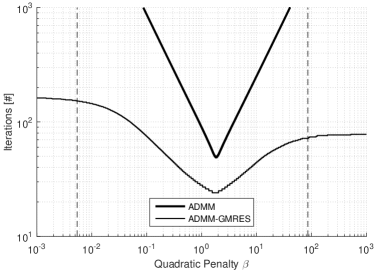
(a)

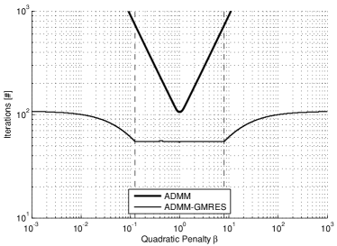
(b)

Figure 1. Convergence of GMRES-accelerated ADMM and regular ADMM with varying $\beta$, and error convergence tolerance $\epsilon=10^{-6}$: (a) randomly generated problem with dimensions $n_{y}=10^{3}$, $n_{x}=2\times 10^{3}$, $n_{z}=300$. The vertical lines mark $m=5.4\times 10^{-3}$ and $\ell=86$ for $\sqrt{m\ell}=0.68$ and $\kappa=\ell/m=1.6\times 10^{4}$; (b) Construction 2 from [34, Sec 6.1], with $n_{y}=n_{x}=10^{3}$, $n_{z}=500$, $\ell=8$, $m=0.125$, $\sqrt{m\ell}=1$, and $\kappa=64$.

When applied to a least-squares problem, ADMM reduces to a classic block Gauss-Seidel splitting on the corresponding KKT equations, i.e. the original saddle-point problem in (1). Viewing ADMM as the resulting linear fixed-point iterations, convergence can be optimally accelerated by using a Krylov subspace method like generalized minimum residual (GMRES) [24, 23]. Or equivalently, viewing ADMM as a preconditioner, it may be used to improve the conditioning of the KKT equations for a Krylov subspace method like GMRES. We refer to the GMRES-accelerated version of ADMM (or the ADMM-preconditioned GMRES) as ADMM-GMRES.

In this paper, we show, using theoretical bounds and empirical results, that ADMM-GMRES (nearly) achieves the optimal convergence rate in (4) for every parameter choice. Figure 1 makes this comparison for two representative problems. Our first main result (Theorem 7) conclusively establishes the optimal iteration bound when $\beta$ is very large or very small. Our second main result (Theorem 9) proves a slightly weaker statement: ADMM-GMRES converges within $O(\kappa^{2/3}\log\epsilon^{-1})$ iterations for all remaining choices of $\beta$, subject to a certain normality assumption. The two bounds gives us the confidence to select the parameter choice $\beta$ in order to maximize numerical stability.

To validate these results, we benchmark the performance of ADMM-GMRES with a randomly selected $\beta$ in Section 7 against regular ADMM with an optimally selected $\beta$. Two problem classes are considered: (1) random problems generated by selecting random orthonormal bases and singular values; and (2) the Newton direction subproblems associated with the interior-point solution of large-scale semidefinite programs. Our numerical results suggest that ADMM-GMRES converges in $O(\sqrt{\kappa}\log\epsilon^{-1})$ iterations for all values of $\beta$, which is a slightly stronger iteration bound that the one we have proved.

1.2. Related ideas

When the optimal parameter choice $\beta$ for (regular) ADMM is explicitly available, we showed in a previous paper [34] that ADMM-GMRES can consistently converge in just $O(\kappa^{1/4}\log\epsilon^{-1})$ iterations, which is an entire order of magnitude better than the optimal bound (4). Problems that would otherwise require thousands of iterations to solve using ADMM are reduced to just tens of ADMM-GMRES iterations. However, the improved rate cannot be guaranteed over all problems, and there exist problem classes where ADMM-GMRES convergences in $\Omega(\sqrt{\kappa}\log\epsilon^{-1})$ iterations for all choices of $\beta$.

More generally, the idea of using a preconditioned Krylov subspace method to solve a saddle-point system has been explored in-depth by a number of previous authors [2, 28, 20, 1, 3, 4]. We make special mention of the Hemitian / Skew-Hermitian (HSS) splitting method, first proposed by Bai, Golub & Ng [1] and used as a preconditioner for saddle-point problems by Benzi & Golub [3], which also makes use of efficient solutions to the subproblems in (2). It is curious to note that HSS has a strikingly similar expression for its optimal parameter choice and the resulting convergence rate, suggesting that the two methods may be closely related.

Note that ADMM is an entirely distinct approach from the augmented Lagrangian / method of multipliers (MM) in optimization, or equivalently, the Uzawa method in saddle-point problems [10, 8]. In MM, convergence is guaranteed in a small, constant number of iterations, but each step requires the solution of an ill-conditioned symmetric positive definite system of equations, often via preconditioned conjugate gradients. In ADMM, convergence is slowly achieved over a large number of iterations, but each iteration is relatively inexpensive. We refer the reader to [7] for a more detailed comparison of the two methods.

Finally, it remains unknown whether these benefits extend to nonlinear saddle-point problems (or equivalently, nonlinear versions of the consensus problem), where the ADMM update equations are also nonlinear. There are a number of competiting approaches to generalize GMRES to nonlinear fixed-point iterations [22, 9, 11]. Their application to ADMM is the subject of future work.

1.3. Definitions & Notation

Given a matrix $M$, we use $\lambda_{i}(M)$ to refer to its $i$-th eigenvalue, and $\Lambda\{M\}$ to denote its set of eigenvalues, including multiplicities. If the eigenvalues are purely-real, then $\lambda_{\max}(M)$ refers to its most positive eigenvalue, and $\lambda_{\min}(M)$ its most negative eigenvalue. Let $\|\cdot\|$ denote the $l_{2}$ vector norm, as well as the associated induced norm, also known as the spectral norm. We use $\sigma_{i}(M)$ to refer to the $i$-th largest singular value.

Define $m=\lambda_{\min}(\tilde{D})$ and $\ell=\lambda_{\max}(\tilde{D})$ as the strong convexity parameter and the gradient Lipschitz constant for the quadratic form associated with the matrix $\tilde{D}=(AD^{-1}A^{T})^{-1}$. The quantity $\kappa=\ell/m$ is the corresponding condition number.

2. Application of ADMM to the Saddle-point Problem

Beginning with a choice of the quadratic-penalty / step-size parameter $\beta>0$ and initial points $\{x^{(0)},z^{(0)},y^{(0)}\}$, the method generates iterates

$$\text{Local var. update: }x^{(k+1)} =\arg\min_{x}\frac{1}{2}x^{T}Dx-r_{x}^{T}x+\frac{\beta}{2}\|Ax+Bz^{(k)}-c+\frac{1}{\beta}y^{(k)}\|^{2},$$

$$\text{Global var. update: }z^{(k+1)} =\arg\min_{z}-r_{z}^{T}z+\frac{\beta}{2}\|Ax^{(k+1)}+Bz-c+\frac{1}{\beta}y^{(k)}\|^{2},$$

$$\text{Multiplier update: }y^{(k+1)} =y^{(k)}+\beta(Ax^{(k+1)}+Bz^{(k+1)}-c).$$

Note that the local and global variable updates can each be implemented by calling one of the two subproblems in (2). Since the KKT optimality conditions are linear with respect to the decision variables, the update equations are also linear, and can be written

(5) $$u^{(k+1)}=G_{\mathrm{AD}}(\beta)u^{(k)}+b(\beta),$$

with iteration matrix

(6) $$G_{\mathrm{AD}}(\beta)=\begin{bmatrix}D+\beta A^{T}A&0&0\\ \beta B^{T}A&\beta B^{T}B&0\\ A&B&-\frac{1}{\beta}I\end{bmatrix}^{-1}\begin{bmatrix}0&-\beta A^{T}B&-A^{T}\\ 0&0&-B^{T}\\ 0&0&-\frac{1}{\beta}I\end{bmatrix},$$

upon the vector of local, global, and multiplier variables, $u^{(k)}=[x^{(k)};z^{(k)};y^{(k)}]$. We will refer to the residual norm in all discussions relating to convergence.

Definition 1 (Residual convergence).

Given the initial and final iterates $u^{(0)}=[x^{(0)};z^{(0)};y^{(0)}]$ and $u^{(k)}=[x^{(k)},z^{(k)},y^{(k)}]$, we say $\epsilon$ residual convergence is achieved in $k$ iterations if $\|Mu^{(k)}-r\|\leq\epsilon\|Mu^{(k)}-r\|$, where $M$ and $r$ are the KKT matrix and vector in (1).

2.1. Basic Spectral Properties

Convergence analysis for linear fixed-point iterations is normally performed by examining the spectral properties of the corresponding iteration matrix. Using dual feasibility arguments, a block-Schur decomposition for (6) can be explicitly specified.

Lemma 2 ([34, Lem. 11]).

Define the QR decomposition $B=QR$ with $Q\in\mathbb{R}^{n_{y}\times n_{z}}$ and $R\in\mathbb{R}^{n_{z}\times n_{z}}$, and define $P\in\mathbb{R}^{p\times(n_{y}-n_{z})}$ as its orthogonal complement. Then defining the orthogonal matrix $U$ and the scaling matrix $S(\beta)$,

(7) $$U=\left[\begin{array}[]{c|cc|c}I_{n_{x}}&0&0&0\\ 0&I_{n_{z}}&0&0\\ 0&0&P&Q\end{array}\right],\qquad S(\beta)=\left[\begin{array}[]{c|cc|c}\beta I_{n_{x}}&0&0&0\\ \hline\cr 0&\beta R&0&0\\ 0&0&I_{n_{y}-n_{z}}&0\\ \hline\cr 0&0&0&I_{n_{z}}\end{array}\right]$$

yields a block-Schur decomposition of $G_{\mathrm{AD}}(\beta)$

(8) $$U^{T}G_{\mathrm{AD}}(\beta)U=S^{-1}(\beta)\left[\begin{array}[]{c|c|c}0_{n_{x}}&G_{12}(\beta)&G_{13}(\beta)\\ \hline\cr 0&G_{22}(\beta)&G_{23}(\beta)\\ \hline\cr 0&0&0_{n_{z}}\end{array}\right]S(\beta),$$

where the size $n_{y}\times n_{y}$ inner iteration matrix $G_{22}(\beta)=\frac{1}{2}I+\frac{1}{2}K(\beta)$ is defined in terms of the matrix

(9) $$K(\beta)=\begin{bmatrix}Q^{T}\\ -P^{T}\end{bmatrix}[(\beta^{-1}\tilde{D}+I)^{-1}-(\beta\tilde{D}^{-1}+I)^{-1}]\begin{bmatrix}Q&P\end{bmatrix},$$

and $\tilde{D}=(AD^{-1}A^{T})^{-1}$.

We may immediately conclude that $G_{\mathrm{AD}}(\beta)$ has $n_{x}+n_{z}$ zero eigenvalues, and $n_{y}$ nonzero eigenvalues the lie within a disk on the complex plane centered at $+\frac{1}{2}$, with radius of $\frac{1}{2}\|K(\beta)\|$. It is straightforward to compute the radius of this disk exactly.

Lemma 3.

Let $\tilde{D}=(AD^{-1}A^{T})^{-1}$, and define $m=\lambda_{\min}(\tilde{D})$ and $\ell=\lambda_{\max}(\tilde{D})$. Then the spectral norm of $K(\beta)$ is given

(10) $$\|K(\beta)\|=\frac{\gamma-1}{\gamma+1},\text{ where }\gamma=\max\left\{\frac{\beta}{m},\frac{\ell}{\beta}\right\}.$$

Also, we see from (8) that each Jordan block associated with a zero eigenvalue of $G_{\mathrm{AD}}(\beta)$ is at most size $2\times 2$. After two iterations, the behavior of ADMM becomes entirely dependent upon the inner iteration matrix $G_{22}(\beta)=\frac{1}{2}I+\frac{1}{2}K(\beta)$.

Lemma 4 ([34, Lem. 13]).

For any $\beta$ and any polynomial $p(\cdot)$, we have

$$\|p(G_{\mathrm{AD}}(\beta))\,G_{\mathrm{AD}}^{2}(\beta)\|\leq c_{1}(\beta)\|p(G_{22}(\beta))\|,$$

where $c_{1}(\beta)$ is defined in terms of the matrices in Lemma 2, as in

$$c_{1}(\beta)=\|S(\beta)\|\|S^{-1}(\beta)\|\|G_{\mathrm{AD}}(\beta)\|^{2}.$$

One application of Lemma 4 is to bound the spectral norm of the $k$-th power iteration, i.e. $\|G_{\mathrm{AD}}^{k}(\beta)\|$, thereby yielding the following iteration estimate.

Proposition 5 ([34, Prop. 7]).

ADMM with fixed parameter $\beta=\sqrt{m\ell}$ attains $\epsilon$ residual convergence in

$$2+\left\lceil(\kappa^{\frac{1}{2}}+1)\log(c_{1}\kappa_{M}\epsilon^{-1})\right\rceil\text{ iterations,}$$

where $c_{1}$ is defined in Lemma 4, and $\kappa_{M}=\|M\|\|M^{-1}\|$ with $M$ defined in (1).

2.2. Accelerating Convergence using GMRES

In the context of quadratic objectives, the convergence of ADMM can be accelerated by GMRES in a largely plug-and-play manner. Given a specific choice of parameter $\beta>0$ and an initial point $u^{(0)}=[x^{(0)};z^{(0)};y^{(0)}]$, we may task GMRES with the fixed-point equation associated with the ADMM update equation (5)

(11) $$u^{\star}-G_{\mathrm{AD}}(\beta)u^{\star}=b(\beta),$$

which is indeed a linear system of equations when $\beta$ is held fixed. It is an elementary fact that the resulting iterates will always converge onto the fixed-point point faster than regular ADMM (under a suitably defined metric) [24].

Alternatively, the fixed-point equation (11) is equivalent to the left-preconditioned system of equations

(12) $$P_{\mathrm{AD}}^{-1}(\beta)[Mu^{\star}-r]=0\qquad\Leftrightarrow\qquad\text{(\ref{eq:admm_fixed})},$$

where $M$ and $r$ are the KKT matrix and residual defined in (1), the ADMM preconditioner matrix is

(13) $$P_{\mathrm{AD}}(\beta)=\begin{bmatrix}I&0&-\beta A^{T}\\ 0&I&-\beta B^{T}\\ 0&0&I\end{bmatrix}\begin{bmatrix}D+\beta A^{T}A&0&0\\ \beta B^{T}A&\beta B^{T}B&0\\ A&B&-\frac{1}{\beta}I\end{bmatrix}=\begin{bmatrix}D&-\beta A^{T}B&A^{T}\\ 0&0&B^{T}\\ A&B&-\frac{1}{\beta}I\end{bmatrix}.$$

Note that the ADMM iteration matrix satisfies $G_{\mathrm{AD}}(\beta)=I-P_{\mathrm{AD}}^{-1}(\beta)M$ by definition. In turn, GMRES-accelerated ADMM is equivalent to a preconditioned GMRES solution to the KKT system, $Mu=r$, with preconditioner $P_{\mathrm{AD}}(\beta)$. Matrix-vector products with $P_{\mathrm{AD}}^{-1}(\beta)$ can always be implemented as the composition of an augmentation operation and a single iteration of ADMM, as seen in the factorization in (13).

GMRES can also be used to solve the right-preconditioned system

(14) $$MP_{\mathrm{AD}}^{-1}(\beta)\hat{u}-r=0,$$

and the solution is recovered via $u=P_{\mathrm{AD}}^{-1}(\beta)\hat{u}$. The resulting method performs essentially the same steps as the one above, but optimizes the iterates under a more preferable metric. Starting from the same initial point $u^{(0)}$, the $k$-th iterate of GMRES as applied to (14), written $u_{\mathrm{GM}}^{(k)}$, is guaranteed to produce a KKT residual norm that is smaller than or equal to that of the $k$-th iterate of regular ADMM, written $u_{\mathrm{AD}}^{(k)}$, as in $\|Mu_{\mathrm{GM}}^{(k)}-r\|\leq\|Mu_{\mathrm{AD}}^{(k)}-r\|$. This property is preferable as $P_{\mathrm{AD}}(\beta)$ becomes progressively ill-conditioned and numerical precision becomes an issue; cf. [34, Sec. 7] for details.

Throughout this paper, we will refer to both methods as GMRES-accelerated ADMM, or ADMM-GMRES for short, and reserve the “left-preconditioned” or the “right-preconditioned” specifications only where the distinctions are important. The reason is that both methods share a common bound for the purposes of convergence analysis.

Proposition 6.

Given fixed $\beta>0$, let $u^{(k)}$ be the iterate generated at the $k$-th iteration of GMRES as applied to either (12) or (14). Then the following bounds hold for all $k\geq 2$

$$\frac{\|Mu^{(k)}-r\|}{\|Mu^{(0)}-r\|}\leq c_{1}\kappa_{P}\min_{\begin{subarray}{c}p\in\mathbb{P}_{k-2}\\ p(1)=1\end{subarray}}\|p(K)\|,$$

where $K\equiv K(\beta)$ is defined in (9), $c_{1}$ is defined in Lemma 4, $\kappa_{P}=\|P_{\mathrm{AD}}\|\|P_{\mathrm{AD}}^{-1}\|$ with $P_{\mathrm{AD}}\equiv P_{\mathrm{AD}}(\beta)$ defined in (13), and $\mathbb{P}_{k}$ denotes the space of order-$k$ polynomials.

Proof.

Given an arbitrary linear system, $Au=b$, GMRES generates iterates $u^{(k)}$ that satisfies the minimal residual property [24]

(15) $$\|r^{(k)}\|/\|r^{(0)}\|\leq\min_{\begin{subarray}{c}p\in\mathbb{P}_{k}\\ p(1)=1\end{subarray}}\|p(I-A)\|,$$

where $r^{(k)}=Au^{(k)}-b$ is the $k$-th residual vector. Furthermore, Lemma 4 yields for all $k\geq 2$,

(16) $$\min_{\begin{subarray}{c}p\in\mathbb{P}_{k}\\ p(1)=1\end{subarray}}\|p(G_{\mathrm{AD}})\|\leq c_{1}\min_{\begin{subarray}{c}p\in\mathbb{P}_{k-2}\\ p(1)=1\end{subarray}}\|p(G_{22})\|=c_{1}\min_{\begin{subarray}{c}p\in\mathbb{P}_{k-2}\\ p(1)=1\end{subarray}}\|p(K)\|,$$

and the last equality is due to the existence of a bijective linear map between $G_{22}\cup\{1\}$ and $K\cup\{1\}$. In the left-preconditioned system (12), the matrix $I-A$ is $I-P_{\mathrm{AD}}^{-1}M=G_{\mathrm{AD}}$, and the $\kappa_{P}$ factor arises by bounding the residuals $\|P_{\mathrm{AD}}r^{(k)}\|/\|P_{\mathrm{AD}}r^{(0)}\|\leq\kappa_{P}\|r^{(k)}\|/\|r^{(0)}\|$. In the right-preconditioned system (12), the matrix $I-A$ is $I-MP_{\mathrm{AD}}^{-1}=P_{\mathrm{AD}}G_{\mathrm{AD}}P_{\mathrm{AD}}^{-1}$, and the $\kappa_{P}$ factor arises via $\|p(P_{\mathrm{AD}}G_{\mathrm{AD}}P_{\mathrm{AD}}^{-1})\|\leq\kappa_{P}\|p(G_{\mathrm{AD}})\|$. ∎

In order to use Proposition 6 to derive useful convergence estimates, the polynomial norm-minimization problem can be reduced into a polynomial min-max approximation problem over a set of points on the complex plane. More specifically, consider the following sequence of inequalities

(17) $$\min_{\begin{subarray}{c}p\in\mathbb{P}_{k}\\ p(1)=1\end{subarray}}\|p(K)\|\leq\min_{\begin{subarray}{c}p\in\mathbb{P}_{k}\\ p(1)=1\end{subarray}}\|Xp(\Lambda)X^{-1}\|\leq\kappa_{X}\min_{\begin{subarray}{c}p\in\mathbb{P}_{k}\\ p(1)=1\end{subarray}}\max_{\lambda\in\Lambda\{K\}}|p(\lambda)|,$$

which makes the following normality assumption, that is standard within this context.

Assumption 1 ($\kappa_{X}$ is bounded).

Given fixed $\beta>0$, the matrix $K\equiv K(\beta)$, defined in (9), is diagonalizable with eigendecomposition, $K=X\Lambda X^{-1}$. Furthermore, the condition number for the matrix-of-eigenvectors, $\kappa_{X}=\|X\|\|X^{-1}\|$, is bounded from above by an absolute constant.

We refer to this last problem in (17) as the eigenvalue approximation problem. Only in very rare cases is an explicit closed-form solution known, but any heuristic choice of polynomial $p(\cdot)$ will provide a valid upper-bound.

3. Convergence Analysis for ADMM-GMRES

Our main result in this paper is that ADMM-GMRES converges to an $\epsilon$-accurate solution in $O(\kappa^{2/3}\log\epsilon^{-1})$ iterations for any value of $\beta>0$, in the sense of the residual. We split the precise statement into two parts. First, for very large and very small values of $\beta$, we can conclusively establish that ADMM-GMRES convergences in $O(\sqrt{\kappa}\log\epsilon^{-1})$ iterations. This is asymptotically the same as the optimal figure for regular ADMM.

Theorem 7 (Extremal $\beta$).

For any choice of $\beta>\ell$ or $0<\beta<m$, GMRES-accelerated ADMM generates the iterate $u^{(k)}=[x^{(k)};z^{(k)};y^{(k)}]$ at the $k$-th iteration that satisfies

$$\frac{\|Mu^{(k)}-r\|}{\|Mu^{(0)}-r\|}\leq 2\,c_{1}\,\kappa_{P}\left[1+\left(\max\left\{\frac{\beta}{\ell},\frac{m}{\beta}\right\}-1\right)^{-1}\right]\left(\frac{\sqrt{2\kappa}-1}{\sqrt{2\kappa}+1}\right)^{0.317\,k}$$

where $\kappa=\ell/m$ and the factors $c_{1},\kappa_{P}$ are polynomial in $\beta+\beta^{-1}$ and defined in Lemma 4 and Proposition 6.

Corollary 8.

GMRES-accelerated ADMM achieves $\epsilon$ residual convergence in

$$O(\sqrt{\kappa}\log\epsilon^{-1}+\sqrt{\kappa}|\log\beta|)\text{ iterations}$$

for any choice of $\beta>\ell$ or $0<\beta<m$.

For intermediate choices of $\beta$, the same result almost holds. Subject to the normality assumption in Assumption 1, ADMM-GMRES converges in $O(\kappa^{2/3}\log\epsilon^{-1})$ iterations. Accordingly, we conclude that ADMM-GMRES converge within this number of iterations for every fixed value of $\beta>0$.

Theorem 9 (Intermediate $\beta$).

For any choice of $m\leq\beta\leq\ell$, GMRES-accelerated ADMM generates the iterate $u^{(k)}=[x^{(k)};z^{(k)};y^{(k)}]$ at the $k$-th iteration that satisfies

$$\frac{\|Mu^{(k)}-r\|}{\|Mu^{(0)}-r\|}\leq 2\,c_{1}\,\kappa_{P}\,\kappa_{X}\left(\frac{\kappa^{2/3}}{\kappa^{2/3}+1}\right)^{0.209\,k}$$

where $\kappa=\ell/m$, the factors $c_{1},\kappa_{P}$ are polynomial in $\beta$ and defined in Lemma 4 and Proposition 6, and the factor $\kappa_{X}$ is defined in Assumption 1.

Corollary 10.

GMRES-accelerated ADMM achieves $\epsilon$ residual convergence in

$$O(\kappa^{2/3}\log\epsilon^{-1}+\kappa^{2/3}|\log\beta|)\text{ iterations}$$

for any choice of $\beta>0$.

As we reviewed in Section 2, convergence analysis for GMRES can be reduced to a polynomial approximation problem over the eigenvalues of $K(\beta)$, written in (17). Our proofs for Theorems 7 & 9 are based on solving this polynomial approximation problem heuristically. The discrete eigenvalue distribution of $K(\beta)$ is enclosed within simple regions on the complex plane in Section 4 for different values of $\beta$. The polynomial approximation problems associated with these outer enclosures are solved in their most general form in Section 5. These results are pieced together in Section 6, yielding proofs to our main results.

4. Eigenvalue Distribution of the Iteration Matrix

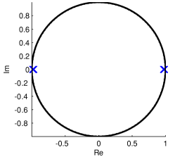
(a)

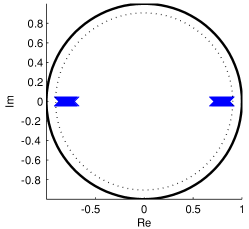
(b)

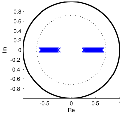
(c)

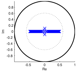
(d)

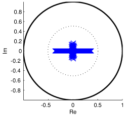
(e)

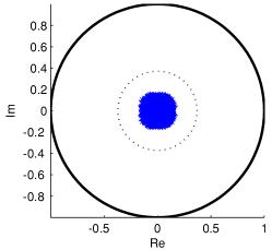
(f)

Figure 2. Eigenvalues (markers) and the spectral norm (dotted circle) of $K(\beta)$ for a randomly generated problem with $n_{y}=n_{x}=1000$, $n_{z}=500$, $m=0.49$ and $\ell=2.2$: (a) $\beta=0.01$; (b) $\beta=0.1$; (c) $\beta=0.33$; (d) $\beta=0.5$; (e) $\beta=0.67$; (f) $\beta=1$. The unit circle is shown in as a solid circle.

The eigenvalues of the iteration matrix $K(\beta)$ play a pivotal role in driving the convergence of both ADMM as well as ADMM-GMRES. Figure 2 plots these for a fixed, randomly generated problem, while sweeping the value of $\beta$. Initially, we see two clusters of purely-real eigenvalues, tightly concentrated about $\pm 1$, that enlargen and shift closer towards the origin and towards each other with increasing $\beta$. As the two clusters coalesce, some of the purely-real eigenvalues become complex. The combined radius of the two clusters reaches its minimum at around $\beta=\sqrt{m\ell}$, at which point most of the eigenvalues are complex. Although not shown, the process is reversed once $\beta$ moves past $\sqrt{m\ell}$; the two clusters shrink, become purely-real, break apart, and move away from the origin, ultimately reverting into two clusters concentrated about $\pm 1$.

Three concrete findings can be summarized from these observations. First, despite the fact that $K(\beta)$ is nonsymmetric, its eigenvalues are purely-real over a broad range of $\beta$.

Lemma 11.

Let $\beta>\ell$ or $\beta<m$. Then $K(\beta)$ is diagonalizable and its eigenvalues are purely real. Furthermore, let $\kappa_{X}$ be the condition number for the matrix-of-eigenvectors as defined in Assumption 1. Then this quantity is bound

(18) $$\kappa_{X}\leq 1+\left(\max\left\{\frac{\beta}{\ell},\frac{m}{\beta}\right\}-1\right)^{-1}.$$

Furthermore, the eigenvalues are partitioned into two distinct, purely-real clusters that only become complex once they coalesce.

Lemma 12.

Define the positive scalar $\gamma=\max\{\beta/m,\ell/\beta\}$, which satisfies $\gamma\geq\sqrt{\kappa}$ by construction. If $\gamma\in[\sqrt{\kappa},\kappa]$, then $\Lambda(K)$ is enclosed within the union of a disk and an interval:

(19) $$\Lambda(K)\subset\left\{z\in\mathbb{C}:|z|\leq\frac{\kappa}{\gamma+\kappa}-\frac{1}{\gamma+1}\right\}\cup\left[-\frac{\gamma-1}{\gamma+1},+\frac{\gamma-1}{\gamma+1}\right].$$

If $\gamma\in(\kappa,2\kappa]$, then $\Lambda(K)$ is enclosed within a single interval:

(20) $$\Lambda(K)\subset\left[-\frac{\gamma-1}{\gamma+1},+\frac{\gamma-1}{\gamma+1}\right].$$

Finally, if $\gamma\in(2\kappa,\infty)$, then $\Lambda(K)$ is enclosed within the union of two disjoint intervals:

(21) $$\Lambda(K)\subset\left[-\frac{\gamma-1}{\gamma+1},-\frac{\gamma-2\kappa}{\gamma+\kappa}\right]\cup\left[+\frac{\gamma-2\kappa}{\gamma+\kappa},+\frac{\gamma-1}{\gamma+1}\right].$$

Furthermore, if $0<n_{x}<n_{y}$, then $\Lambda(K)$ contains at least one eigenvalue within each interval.

In the limits $\beta\to 0$ and $\beta\to\infty$, the two clusters in (21) concentrate about $\pm 1$, and the spectral radius of the ADMM iteration matrix converges towards 1.

Corollary 13.

Let $\beta>2\ell$ or $\beta<\frac{1}{2}m$. Then for $0<n_{z}<n_{y}$, there exists an eigenvalue of the ADMM iteration matrix $\lambda_{i}\in\Lambda\{G_{\mathrm{AD}}(\beta)\}$ whose modulus is lower-bounded

$$|\lambda_{i}|\geq\frac{\gamma-\kappa}{\gamma+\kappa},\text{ where }\gamma=\max\left\{\frac{\beta}{m},\frac{\ell}{\beta}\right\}.$$

The spectral radius determines the asympotic convergence rate, so given Corollary 13, it is unsurprising that ADMM stagnates if $\beta$ is poorly chosen. But the situation is different with ADMM-GMRES, because it is able to exploit the clustering of eigenvalues. As we will see later, this is the mechanism that allows ADMM-GMRES to be insensitive to the parameter choice.

4.1. Properties of $J$-symmetric matrices

Most of our characterizations for the eigenvalues of $K(\beta)$ are based on a property known as “$J$-symmetry”. In the following discussion, we will drop all arguments with respect to $\beta$ for clarity. Returning to its definition in (9), we note that $K$ has the block structure

(22) $$K=\begin{bmatrix}X&Z\\ -Z^{T}&Y\end{bmatrix},$$

with subblocks $X\in\mathbb{R}^{n_{z}\times n_{z}}$, $Y\in\mathbb{R}^{(n_{y}-n_{z})\times(n_{y}-n_{z})}$, and $Z\in\mathbb{R}^{n_{z}\times(n_{y}-n_{z})}$,

(23) $$X=Q^{T}\tilde{K}Q,\qquad Y=-P^{T}\tilde{K}P,\qquad Z=Q^{T}\tilde{K}P,$$

(24) $$\tilde{K}=(\beta^{-1}\tilde{D}+I)^{-1}-(\beta\tilde{D}^{-1}+I)^{-1},$$

and the matrices $Q$ and $P$ with orthonormal columns are defined as in Lemma 2. From the block structure in (22) we see that the matrix $K$ is self-adjoint with respect to the indefinite product (assuming $0<n_{z}<n_{y}$) defined by $J=\mathrm{blkdiag}(I_{n_{z}},-I_{(n_{y}-n_{z})})$:

$$\left\langle y,Mx\right\rangle_{J}=\left\langle My,x\right\rangle_{J}\qquad\iff\qquad y^{T}JMx=(My)^{T}Jx.$$

Matrices that have this property frequently appear in saddle-point type problems; cf. [4, 5] for a more detailed treatment of this subject. Much can be said about their spectral properties.

Proposition 14.

The $J$-symmetric matrix $K$ in (22) has at most $2\min\{n_{z},n_{y}-n_{z}\}$ eigenvalues with nonzero imaginary parts, counting conjugates. These eigenvalues are contained within the disk $\mathcal{D}_{a}=\{z\in\mathbb{C}:|z|\leq a\}$ of radius

$$a=\min_{\eta\in\mathbb{R}}\|K+\eta J\|,$$

where $\mathbb{P}$ denotes the space of polynomials.

Proof.

Benzi & Simoncini [5] provide a succinct proof for the first statement. The second statement is based on the fact that every eigenpair $\{\lambda_{i},x_{i}\}$ of $K$ satisfying $\mathrm{Im}(\lambda_{i})\neq 0$ must have an eigenvector $x_{i}$ that is “$J$-neutral”, i.e. satisfying $x_{i}^{*}Jx_{i}=0$; cf. [5, Thm. 2.1]. Hence, the following bound holds

(25) $$|\lambda_{i}|\leq\max_{\|x\|=1}\{|x^{*}Kx|:x^{*}Jx=0\}$$

for every $\lambda_{i}$ with $\mathrm{Im}(\lambda_{i})\neq 0$. Taking the Lagrangian dual of (25) yields the desired statement. ∎

Also, we can derive a simple sufficient condition for the eigenvalues of $K$ to be purely real, based on the ideas described in [5].

Proposition 15.

Suppose that there exists a real scalar $\eta\neq 0$ to make the matrix $H=\eta JK$ positive definite. Then $K$ is diagonalizable with eigendecomposition, $K=X\Lambda X^{-1}$, its eigenvalues are purely-real, and the condition number of the matrix-of-eigenvectors satisfies $\kappa_{X}\triangleq\|X\|\|X^{-1}\|\leq\sqrt{\|H\|\|H^{-1}\|}$

Proof.

It is easy to verify that $K$ is also symmetric with respect to $H$, as in $KM=K^{T}H$. Since $H$ is positive definite, there exists a symmetric positive definite matrix $W=W^{T}$ satisfying $W^{2}=H$, and the $H$-symmetry implies

$$W(WMW^{-1})W=W(W^{-1}M^{T}W)W\quad\iff\quad WMW^{-1}=(WMW^{-1})^{T}=\tilde{M}.$$

Hence we conclude that $M$ is similar to the real symmetric matrix $\tilde{M}$, with purely-real eigenvalues and eigendecomposition $\tilde{M}=V\Lambda V^{T}$, where $V$ is orthogonal. The corresponding eigendecomposition for $M$ is $M=X\Lambda X^{-1}$ with $X=W^{-1}V$. ∎

Finally, we may use the block-generalization of Gershgorin’s circle theorem to decide when the off-diagonal block $Z$ is sufficiently “small” such that the eigenvalues of $K$ become similar to the block diagonal matrix $\mathrm{blkdiag}(X,Y)$.

Proposition 16.

Given $J$-symmetric matrix $K$ in (22), define the two Gershgorin sets

$$\mathcal{G}_{X}=\bigcup_{i=1}^{n}\{z\in\mathbb{C}:|z-\lambda_{i}(X)|\leq\|Z\|\},\qquad\mathcal{G}_{Y}=\bigcup_{i=1}^{m}\{z\in\mathbb{C}:|z-\lambda_{i}(Y)|\leq\|Z\|\}.$$

Then $\Lambda\{K\}\subset\mathcal{G}_{X}\cup\mathcal{G}_{Y}$. Moreover, if $\mathcal{G}_{X}$ and $\mathcal{G}_{Y}$ are disjoint, i.e. $\mathcal{G}_{X}\cap\mathcal{G}_{Y}=\emptyset$, then $\Lambda\{K\}$ contains exactly $n_{z}$ eigenvalues in $\mathcal{G}_{X}$ and $n_{y}-n_{z}$ eigenvalues in $\mathcal{G}_{Y}$.

Proof.

This is a straightforward application of the block Gershgorin’s theorem for matrices with normal pivot blocks [12, Thm. 4]. ∎

4.2. Proof of Lemma 11

Proof.

The cases of $n_{z}=0$ and $n_{z}=n_{y}$ are trivial. In the remaining cases, $K$ is $J$-symmetric, and we will use Proposition 15 to prove the statement. Noting that $JK$ is unitarily similar with $\tilde{K}$, simple direct computation reveals that $+JK$ is positive definite for $\beta>\ell$, and $-JK$ is positive definite for $\beta<m$. Hence, for these choices of $\beta$, the eigenvalues of $K$ are purely real. Some further computation reveals that $\|JK\|=(\gamma-1)/(\gamma+1)$ and $\|(JK)^{-1}\|=(\gamma+\kappa)/(\gamma-\kappa)$, so the condition number of $JK$ is bound

(26) $$\|JK\|\|(JK)^{-1}\|<\|(JK)^{-1}\|=\frac{\gamma+\kappa}{\gamma-\kappa}=1+\frac{2}{\gamma/\kappa-1}.$$

Taking the square-root and substituting $\sqrt{1+2x}\leq 1+x$ yields the desired estimate for $\kappa_{X}$ in (18). ∎

4.3. Proof of Lemma 12

Proof.

Again, the cases of $n_{z}=0$ and $n_{z}=n_{y}$ are trivial. In all remaining cases, $K$ is $J$-symmetric. The single interval case (20) is a trivial consequence of our purely-real result in Lemma 11. The disk-and-interval case (19) arises from Proposition 14, in which we use the disk of radius

$$a=\min_{\eta\in\mathbb{R}}\|K-\eta J\|=\min_{\eta\in\mathbb{R}}\|\tilde{K}-\eta I\|=\frac{\kappa}{\gamma+\kappa}-\frac{1}{\gamma+1}$$

to enclose the eigenvalues with nonzero imaginary parts, and the spectral norm disk $|\lambda_{i}(K)|\leq\|K\|$ to enclose the purely-real eigenvalues. The two-interval case (21) is a consequence of the block Gershgorin theorem in Proposition 16. Some direct computation on the block matrices in (22) yields the following two statements

(27) $$\Lambda\{X\}\cup\Lambda\{Y\} \subset\left[-\frac{\gamma-1}{\gamma+1},-\frac{\gamma-\kappa}{\gamma+\kappa}\right]\cup\left[+\frac{\gamma-\kappa}{\gamma+\kappa},+\frac{\gamma-1}{\gamma+1}\right]\subset\mathbb{R},$$

(28) $$\|Z\| \leq\frac{\kappa}{\gamma+\kappa},$$

the latter of which also uses the fact that $\|Q^{T}\tilde{K}P\|=\|Q^{T}(\tilde{K}-\eta I)P\|\leq\|\tilde{K}-\eta I\|$. The projections of the corresponding Gershgorin regions onto the real line satisfy

$$\mathrm{Re}\{\mathcal{G}_{-}\}\subset\left[-\frac{\gamma-1}{\gamma+1}-\frac{\kappa}{\gamma+\kappa},-\frac{\gamma-2\kappa}{\gamma+\kappa}\right],\quad\mathrm{Re}\{\mathcal{G}_{+}\}\subset\left[\frac{\gamma-2\kappa}{\gamma+\kappa},\frac{\gamma-1}{\gamma+1}+\frac{\kappa}{\gamma+\kappa}\right].$$

Once $\gamma>2\kappa$, the regions become separated. Taking the intersection between each disjoint Gershgorin region, the real line, and the spectral norm disk $|\lambda_{i}(K)|\leq\|K\|$ yields (21). ∎

5. Solving the Approximation Problems

With the distribution of eigenvalues characterized in Lemma 12, we now consider solving each of the three accompanying approximation problems in their most general form.

5.1. Chebyshev approximation over the real interval

The optimal approximation for an interval over the real line has a closed-form solution due to a classic result attributed to Chebyshev.

Theorem 17.

Let $\mathcal{I}$ denote the interval $[c-a,c+a]$ on the real line. Then assuming that $+1\notin\mathcal{I}$, the polynomial approximation problem has closed-form solution

(29) $$\min_{\begin{subarray}{c}p\in\mathbb{P}_{k}\\ p(1)=1\end{subarray}}\max_{z\in\mathcal{I}}|p(z)|=\frac{1}{|T_{k}(\frac{1-c}{a})|}\leq 2\left(\frac{\sqrt{\kappa_{I}}-1}{\sqrt{\kappa_{I}}+1}\right)^{k},$$

where $T_{k}(z)$ is the degree-$k$ Chebyshev polynomial of the first kind, and $\kappa_{I}=(|1-c|+a)/(|1-c|-a)$ is the condition number for the interval. The minimum is attained by the Chebyshev polynomial $p^{\star}(z)=T_{k}(\frac{z-c}{a})/|T_{k}(\frac{1-c}{a})|$.

Proof.

See e.g. [21]. ∎

Whereas approximating a general $\kappa$-conditioned region to $\epsilon$-accuracy requires an order $O(\kappa\log\epsilon^{-1})$ polynomial, approximating a real interval of the same conditioning and to the same accuracy only requires an order $O(\sqrt{\kappa}\log\epsilon^{-1})$ polynomial. This is the underlying mechanism that grants the conjugate gradients method a square-root factor speed-up over gradient descent; cf. [16, Ch. 3] for a more detailed discussion. For future reference, we also note the following identity.

Remark 18.

Given any $\zeta>+1$, define the corresponding condition number as $\nu=(\zeta+1)/(\zeta-1)$. Then

(30) $$|\zeta|^{k}=\left(\frac{\nu+1}{\nu-1}\right)^{k},\qquad\frac{1}{2}\left(\frac{\sqrt{\nu}+1}{\sqrt{\nu}-1}\right)^{k}\leq|T_{k}(\zeta)|\leq\left(\frac{\sqrt{\nu}+1}{\sqrt{\nu}-1}\right)^{k}.$$

5.2. Real intervals symmetric about the imaginary axis

Now, consider the polynomial approximation problem for two real, non-overlapping intervals with respect to the constraint point $+1$, illustrated in Fig. 3, which arises as the eigenvalue distribution (21) in Lemma 12.

Lemma 19.

Given $a\geq 0$ and $c\geq a$, define the two closed intervals

(31) $$\mathcal{I}_{-}=\{z\in\mathbb{R}:|z+c|\leq a\},\qquad\mathcal{I}_{+}=\{z\in\mathbb{R}:|z-c|\leq a\},$$

such that $+1\notin I_{+}$ and $\mathcal{I}_{-}\cap\mathcal{I}_{+}=\emptyset$. Then the following holds

(32) $$\left(\frac{\sqrt{\kappa_{+}}+1}{\sqrt{\kappa_{+}}-1}\right)^{k}\leq\min_{\begin{subarray}{c}p\in\mathbb{P}_{k}\\ p(1)=1\end{subarray}}\max_{z\in\mathcal{I}_{-}\cup\mathcal{I}_{+}}|p(z)|\leq 2\left(\frac{\sqrt{\kappa_{+}}+1}{\sqrt{\kappa_{+}}-1}\right)^{0.317\,k}$$

where $\kappa_{+}=(1-c+a)/(1-c-a)$ is the condition number for the segment $\mathcal{I}_{+}$.

Of course, the union of the two intervals, i.e. $\mathcal{I}_{-}\cup\mathcal{I}_{+}$, lies within a single real interval with condition number $\kappa_{I}=(1+c+a)/(1-c-a)$, so Theorem 17 can also be used to obtain an estimate. However, the explicit treatment of clustering in Lemma 19 yields a considerably tighter bound, because it is entirely possible for each $\mathcal{I}_{-}$ and $\mathcal{I}_{+}$ to be individually well-conditioned while admitting an extremely ill-conditioned union. For a concrete example, consider setting $a=0$ and taking the limit $c\to 1$; the condition number for $\mathcal{I}_{+}$ is fixed at $\kappa_{+}=1$, but the condition number for the union $\mathcal{I}_{-}\cup\mathcal{I}_{+}$ diverges $\kappa_{I}\to\infty$. In this case, Lemma 19 predicts extremely rapid convergence for all values of $c$, whereas Theorem 17 does not promise convergence at all.

Figure 3. Real intervals symmetric about the imaginary axis.

To prove Lemma 19, we will begin by stating a technical lemma.

Lemma 20.

Define $f(x)=\log[(x-1)/(x+1)]$ with domain $x\in(1,\infty)$. Then the quotient $g(x)=f(x)/f(x^{2})$ is monotonously increasing with infimum attained at the limit point $g(1)=1$.

Proof.

By definition, we see that both $f(x)$ and $f(x^{2})$ are nonzero for all $x>1$. Taking the derivatives

(33) $$\frac{d}{dx}\left[f(x)\right]=\frac{2}{x^{2}-1}=\frac{2x^{2}+2}{x^{4}-1},\qquad\frac{d}{dx}\left[f(x^{2})\right]=\frac{4x}{x^{4}-1},$$

reveals that $f(x)$ is monotonously increasing for all $x>1$, so we also have $f(x)<f(x^{2})$. Finally, we observe that $\frac{d}{dx}\left[f(x)\right]>\frac{d}{dx}\left[f(x^{2})\right]>0$ for all $x>1$. Combining these three observations with the quotient rule reveals that $g(x)$ is monotonously increasing

(34) $$\frac{d}{dx}\left[g(x)\right]=\frac{f(x^{2})\,\frac{d}{dx}\left[f(x)\right]-f(x)\,\frac{d}{dx}\left[f(x^{2})\right]}{[f(x^{2})]^{2}}>0\qquad\forall x>1.$$

Hence, the infimum for $g(x)$ must be attain at its lower limit point $x=1$. Using l’Hôpital’s rule yields $\lim_{x\to 1}g(x)=\lim_{x\to 1}(2x^{2}+2)/(4x)=1$. ∎

Proof of Lemma 19.

For the lower-bound, we have via Theorem 17 and Remark 18

$$\min_{\begin{subarray}{c}p\in\mathbb{P}_{k}\\ p(1)=1\end{subarray}}\max_{z\in\mathcal{I}_{-}\cup\mathcal{I}_{+}}|p(z)|\geq\min_{\begin{subarray}{c}p\in\mathbb{P}_{k}\\ p(1)=1\end{subarray}}\max_{z\in\mathcal{I}_{+}}|p(z)|=\frac{1}{T_{k}(\frac{1-c}{a})}\geq\left(\frac{\sqrt{\kappa_{+}}+1}{\sqrt{\kappa_{+}}-1}\right)^{k}.$$

For the upper-bound, consider the product of an order-$\xi$ Chebyshev polynomial over $\mathcal{I}_{+}$ and an order-$\eta$ monomial over $\mathcal{I}_{-}$, as in

(35) $$p(z)=\left(\frac{z+c}{1+c}\right)^{\eta}\frac{T_{\xi}(\frac{z-c}{a})}{|T_{\xi}(\frac{1-c}{a})|},$$

with infinity norms $\|p(z)\|_{\mathcal{I}_{-}}\triangleq\max_{z\in\mathcal{I}_{-}}|p(z)|$ and $\|p(z)\|_{\mathcal{I}_{+}}\triangleq\max_{z\in\mathcal{I}_{+}}|p(z)|$ attained at $z=-(c+a)$ and $z=+(c+a)$ respectively

(36) $$\|p(z)\|_{\mathcal{I}_{-}}=\left(\frac{a}{1+c}\right)^{\eta}\frac{|T_{\xi}(\frac{a+2c}{a})|}{|T_{\xi}(\frac{1-c}{a})|},\qquad\|p(z)\|_{\mathcal{I}_{+}}=\left(\frac{a+2c}{1+c}\right)^{\eta}\frac{1}{|T_{\xi}(\frac{1-c}{a})|}.$$

We choose the exponents $\eta+\xi=k$ in the ratio

(37) $$\eta/\xi =\log\left(\frac{\sqrt{\nu}-1}{\sqrt{\nu}+1}\right)\bigg{/}\log\left(\frac{\nu-1}{\nu+1}\right),$$

in which $\nu=1+a/c$ is the condition number of the well-conditioned interval $\mathcal{I}_{-}$ with respect to the ill-conditioned interval $\mathcal{I}_{+}$. This particular ratio implies

(38) $$\left(\frac{\nu-1}{\nu+1}\right)^{\eta}=\left(\frac{\sqrt{\nu}-1}{\sqrt{\nu}+1}\right)^{\xi}\qquad\implies\qquad\left(\frac{a}{a+2c}\right)^{\eta}\leq\frac{1}{|T_{\xi}(\frac{a+2c}{a})|},$$

via the bounds in Remark 18, so $\|p(z)\|_{\mathcal{I}_{+}}\geq\|p(z)\|_{\mathcal{I}_{-}}$ is satisfied by construction, and the global error bound is bound

(39) $$\max_{z\in\mathcal{I}_{-}\cup\mathcal{I}_{+}}|p(z)|\leq\|p(z)\|_{\mathcal{I}_{+}}\leq 2\left(\frac{\sqrt{\kappa_{+}}+1}{\sqrt{\kappa_{+}}-1}\right)^{\xi}.$$

To complete the proof, we require a lower estimate of $\xi$ in terms of $k$ that is valid for any valid of $a$ and $c$, or equivalently, any value of $\nu$. Since $k=\eta+\xi$ by definition, the ratio is written $\xi/k=1/(1+\eta/\xi)$, so we really desire an upper estimate on the ratio $\eta/\xi$ defined in (37). According to Lemma 20, the quotient in (37) is monotonously increasing with respect to $\sqrt{\nu}$. Hence, the maximum value of $\eta/\xi$ is attained at the maximum value of $\nu$. The choice of $a=c$ maximizes $\nu$ with maximum at $v=2$, since any choice of $a>c$ would cause $\mathcal{I}_{-}$ and $\mathcal{I}_{+}$ to overlap. Evaluating the expression at $\nu=2$ yields $\eta/\xi\leq\log\left(\frac{\sqrt{2}-1}{\sqrt{2}+1}\right)\bigg{/}\log\left(\frac{2-1}{2+1}\right)\leq 2.151$. This implies $\xi/k=1/(1+\eta/\xi)\geq 1/3.151=0.317$. ∎

5.3. Concentric disk and interval

Figure 4. Disk-and-interval eigenvalue distribution.

Finally, consider the polynomial approximation problem for the union of a disk and a real interval with respect to the constraint point $+1$, illustrated in Fig. 4, which arises as the eigenvalue distribution (19) in Lemma 12.

Lemma 21.

Given $0\leq a_{D}\leq a_{I}<1$, define the disk $\mathcal{D}=\{z\in\mathbb{C}:|z|\leq a_{D}\}$ and the interval $\mathcal{I}=\{z\in\mathbb{C}:|z|\leq a_{I}\}$. Then

(40) $$\min_{\begin{subarray}{c}p\in\mathbb{P}_{k}\\ p(1)=1\end{subarray}}\max_{z\in\mathcal{D}\cup\mathcal{I}}|p(z)|\leq 2\left(\frac{\kappa_{I}-1}{\kappa_{I}+1}\right)^{\eta}\left(\frac{\sqrt{\kappa_{I}}-1}{\sqrt{\kappa_{I}}+1}\right)^{\xi}.$$

where $\kappa_{I}=(1+a_{I})/(1-a_{I})$ is the condition number for the interval, and $\eta+\xi=k$ are defined

$$\eta=\left\lceil\frac{c_{0}}{\delta+c_{0}}\right\rceil,\qquad\xi=\left\lfloor\frac{\delta}{\delta+c_{0}}\right\rfloor$$

where $\delta=1-a_{D}/a_{I}$ and $c_{0}=\log(1+\sqrt{2})\approx 0.8814$.

It is easy to verify that $\kappa_{I}$ is also the condition number for the union of the disk and the interval, $\mathcal{D}\cup\mathcal{I}$. Consequently, one interpretation of Lemma 21 is that there exists an order $O(\sqrt{\kappa}\log\epsilon^{-1})$ polynomial that approximates a $\kappa$-conditioned version of $\mathcal{D}\cup\mathcal{I}$ to $\epsilon$-accuracy, but only so long as the disk $\mathcal{D}$ is strictly better conditioned than the interval $\mathcal{I}$. If $a_{D}=a_{I}$, then both regions share the same condition number, and the square-root factor speed-up is lost; an order $O(\kappa\log\epsilon^{-1})$ polynomial is now required to solve the same approximation problem.

The proof of Lemma 21 requires the following estimate on the value of the Chebyshev polynomial over the complex plane.

Proposition 22.

The maximum modulus of the $k$-th order Chebyshev polynomial is bound within the disk on the complex plane centered at the origin with radius $\eta$,

(41) $$\max_{|z|\leq\eta}|T_{k}(z)|\leq T_{k}(\sqrt{1+\eta^{2}})\leq\left(\eta+\sqrt{1+\eta^{2}}\right)^{k},$$

and the first inequality is tight for $k$ even.

Proof.

The maximum modulus for $T_{k}(z)$ over the ellipse with unit focal distance and principal axis $a\geq\eta$ are attained at $2n$ points along its boundary the points [21, 24]

(42) $$z_{k}=a\cos\left(\frac{k\pi}{n}\right)+j\sqrt{a^{2}-1}\sin\left(\frac{k\pi}{n}\right)\qquad k=1,\ldots,2n.$$

The ellipse with $a=\sqrt{1+\eta^{2}}$ is the smallest to enclose the disk of radius $\eta$, and if $k$ is even, then $z_{k/2}$ also lies on its boundary. The second bound follows by definition

(43) $$T_{k}(\sqrt{1+\eta^{2}})=\frac{1}{2}\left(\eta+\sqrt{1+\eta^{2}}\right)^{k}+\frac{1}{2}\left(\eta+\sqrt{1+\eta^{2}}\right)^{-k}\leq\left(\eta+\sqrt{1+\eta^{2}}\right)^{k}.$$

∎

Proof of Lemma 21.

Consider the product of an order-$\xi$ Chebyshev polynomial over $\mathcal{I}_{+}$ and an order-$\eta$ monomial over $\mathcal{I}_{-}$, as in

(44) $$p(z)=\left(\frac{z/a_{D}}{1/a_{D}}\right)^{\eta}\frac{T_{\xi}(z/a_{I})}{|T_{\xi}(1/a_{I})|}=z^{\eta}\,\frac{T_{\xi}(z/a_{I})}{|T_{\xi}(1/a_{I})|},$$

with infinity norms $\|p(z)\|_{\mathcal{D}}\triangleq\max_{z\in\mathcal{D}}|p(z)|$ and $\|p(z)\|_{\mathcal{I}}\triangleq\max_{z\in\mathcal{I}}|p(z)|$ given

(45) $$\|p(z)\|_{\mathcal{D}}=\frac{a_{D}^{\eta}\,\|T_{\xi}(z/a_{I})\|_{\mathcal{D}}}{|T_{\xi}(1/a_{I})|}\leq\frac{a_{D}^{\eta}(1+\sqrt{2})^{\xi}}{|T_{\xi}(1/a_{I})|},\qquad\|p(z)\|_{\mathcal{I}}=\frac{a_{I}^{\eta}}{|T_{\xi}(1/a_{I})|}.$$

The bound $(1+\sqrt{2})^{\xi}\geq\max_{|z|\leq 1}|T_{\xi}(z)|\geq\|T_{\xi}(z/a_{I})\|_{\mathcal{D}}$ arises from $a_{D}\leq a_{I}$ and Proposition 22. Choosing the exponents $\eta$ and $\xi$ to satisfy the ratio

(46) $$\eta/\xi=\frac{\log(1+\sqrt{2})}{1-a_{D}/a_{I}}\geq\frac{\log(1+\sqrt{2})}{\log(a_{I}/a_{D})}\qquad\implies\qquad\left(\frac{a_{D}}{a_{I}}\right)^{\eta}\leq\frac{1}{(1+\sqrt{2})^{\xi}},$$

satisfies $\|p(z)\|_{\mathcal{D}}\leq\|p(z)\|_{\mathcal{I}}$ by construction, so the global error is bound by $\|p(z)\|_{\mathcal{I}}$. Bounding the term $1/|T_{\xi}(1/a_{I})|$ in $\|p(z)\|_{\mathcal{I}}$ with Remark 18 completes the result. ∎

6. Proof of the Main Results

With the eigenvalues of $K(\beta)$ characterized and the corresponding approximation problems solved, we are now ready to prove our main results.

6.1. Regime of purely-real eigenvalues

Loosely speaking, Theorem 7 states that for parameter values of $\beta>\ell$ or $\beta<m$, ADMM-GMRES is guaranteed to converge to an $\epsilon$-accurate solution in $O(\sqrt{\kappa}\log\epsilon^{-1})$ iterations. We will prove this statement by solving the $K(\beta)$ eigenvalue approximation problem associated for $\beta>\ell$ or $\beta<m$ heuristically, using Theorem 17 and Lemma 19, and substituting the resulting bound into Proposition 6. This two-step process begins with the following bound.

Lemma 23.

Let $\beta>\ell$ or $\beta<m$. Then the eigenvalue approximation problem for $K(\beta)$ has bounds

(47) $$\min_{\begin{subarray}{c}p\in\mathbb{P}_{k}\\ p(1)=1\end{subarray}}\max_{\lambda\in\Lambda\{K(\beta)\}}|p(\lambda)|\leq 2\left(\frac{\sqrt{2\kappa}-1}{\sqrt{2\kappa}+1}\right)^{0.317\,k}.$$

Proof.

First, we consider $\beta\in[\frac{1}{2}m,m)\cup(\ell,2\ell]$. According to (20) in Lemma 12, the eigenvalues of $K(\beta)$ are distributed over a purely-real interval bounded by $\|K(\beta)\|=(\gamma-1)/(\gamma+1)$, where $\gamma=\max\{\beta/m,\ell/\beta\}$ lies $\gamma\in(\kappa,2\kappa]$. The associated condition number $\kappa_{I}=\gamma$ is bounded $\kappa<\kappa_{I}\leq 2\kappa$, and applying the Chebyshev polynomial approximation in Theorem 17 yields a less conservative version of (47), i.e. one with a larger exponent on the upper-bound.

Next, we consider the remaining choices, $\beta>2\ell$ or $\beta<\frac{1}{2}m$. According to (21) in Lemma 12, the eigenvalues of $K(\beta)$ are clustered along two non-overlapping intervals, symmetric about the imaginary axis. The condition number for the interval lying in the right-half plane is $\kappa_{+}=\frac{3}{2}\kappa(\gamma+1)/(\gamma+\kappa)$ with $\gamma>2\kappa$, so its value is bound $\kappa<\kappa_{+}\leq 2\kappa$. Making this substitution into the heuristic solution for the two-segment problem in Lemma 19 yields exactly (47). ∎

According to Lemma 47, solving the $K(\beta)$ eigenvalue approximation problem (for $\beta>\ell$ or $\beta<m$) to $\epsilon$-accuracy will require a polynomial of order $\approx 2.2\sqrt{\kappa}\log\epsilon^{-1}$, where the leading constant is $2.2\approx\sqrt{2}/(2\times 0.317)$. Assuming that the eigenvalue characterizations (20) and (21) in Lemma 12 are sharp, this figure cannot be improved by more than a small absolute constant. This is because all other ingredients in the proof of Lemma 23 have approximation constants no greater than 4.

Proof of Theorem 7.

Substituting the bound on the eigenvalue approximation problem in Lemma 23 and the bound on the condition number for the matrix-of-eigenvectors in Lemma 11 into Proposition 6 yields the desired statement. ∎

6.2. Regime of complex eigenvalues

Loosely speaking, Theorem 7 states that for parameter values of $m\leq\beta\leq\ell$, ADMM-GMRES is guaranteed to converge to an $\epsilon$-accurate solution in $O(\kappa^{2/3}\log\epsilon^{-1})$ iterations. We will prove this statement by solving the $K(\beta)$ eigenvalue approximation problem heuristically using Lemma 21, estimating a bound on the resulting convergence factor that is independent of $\beta$, and substituting the bound into Proposition 6.

To begin, Lemma 12 says that for $\beta\in[m,\ell]$, the eigenvalues of $K(\beta)$ are distributed over the union of a disk and an interval. Lemma 21 can be used to provide a heuristic solution for this eigenvalue distribution. Substituting the former into the latter yields

(48) $$\min_{\begin{subarray}{c}p\in\mathbb{P}_{k}\\ p(1)=1\end{subarray}}\max_{\lambda\in K(\beta)}|p(\lambda)|\leq 2\rho^{k},$$

where the convergence factor and associated parameters are

(49) $$\rho(\gamma)=\left(\frac{\gamma-1}{\gamma+1}\right)^{\frac{c_{0}}{c_{0}+\delta}}\left(\frac{\sqrt{\gamma}-1}{\sqrt{\gamma}+1}\right)^{\frac{\delta}{c_{0}+\delta}},\qquad\delta(\gamma)=\frac{\gamma^{2}-\kappa}{(\gamma+\kappa)(\gamma+1)}$$

and $c_{0}=\log(1+\sqrt{2})$. Recall that $\gamma=\max\{\beta/m,\ell/\beta\}$.

Lemma 24.

Let $\sqrt{\kappa}\leq\gamma\leq\kappa$, and define $\delta(\gamma)$ as a function of $\gamma$ as in (49). Then

(50) $$\left(\frac{\gamma-1}{\gamma+1}\right)^{\frac{c_{0}}{c_{0}+\delta(\gamma)}}\left(\frac{\sqrt{\gamma}-1}{\sqrt{\gamma}+1}\right)^{\frac{\delta(\gamma)}{c_{0}+\delta(\gamma)}}\leq\left(1-\frac{1}{\kappa^{2/3}+1}\right)^{0.209\,k}.$$

Proof.

We will attempt to lower-bound the logarithm of (50) by applying $\log(1+x)\leq x$, as in

(51) $$-\frac{1}{2}\log\rho\geq\frac{c_{0}}{c_{0}+\delta(\gamma)}\left(\frac{1}{\gamma+1}\right)+\frac{\delta(\gamma)}{c_{0}+\delta(\gamma)}\left(\frac{1}{\sqrt{\gamma}+1}\right).$$

Directly substituting $\delta(\gamma)$ from (49) into (51) and sweeping $\gamma=\kappa^{\alpha}$ over $\alpha\in[0.5,1]$ yields

(52) $$\text{(\ref{eq:proof_thm_log_conv_fac})}= \frac{c_{0}^{-1}\kappa^{2\alpha}+\kappa^{1.5\alpha}+\kappa^{\alpha}+\kappa^{0.5\alpha+1}-(c_{0}^{-1}-1)\kappa}{\left(\kappa^{0.5\alpha}+1\right)\left((c_{0}^{-1}+1)\kappa^{2\alpha}+\kappa^{\alpha}+\kappa^{\alpha+1}-(c_{0}^{-1}-1)\kappa\right)}$$

(53) $$= \frac{c_{0}^{-1}\kappa^{0.5\alpha-1}+\kappa^{-1}+\kappa^{-0.5\alpha-1}+\kappa^{-\alpha}-(c_{0}^{-1}-1)\kappa^{-1.5\alpha}}{\left(1+\kappa^{-0.5\alpha}\right)\left((c_{0}^{-1}+1)\kappa^{\alpha-1}+\kappa^{-1}+1-(c_{0}^{-1}-1)\kappa^{-\alpha}\right)}$$

(54) $$\geq \frac{c_{0}^{-1}\kappa^{0.5\alpha-1}+0+0+\kappa^{-\alpha}-(c_{0}^{-1}-1)\kappa^{-1.5\alpha}+0}{\left(1+1\right)\left((c_{0}^{-1}+1)+1+1\right)}$$

(55) $$= \frac{c_{0}^{-1}\kappa^{0.5\alpha-1}+\kappa^{-\alpha}-(c_{0}^{-1}-1)\kappa^{-1.5\alpha}}{2(c_{0}^{-1}+3)}$$

where (52)$\Rightarrow$(53) divides the numerator and denominator by $\kappa^{1.5\alpha+1}$, and (53)$\Rightarrow$(54) uses the fact that $\kappa\geq 1$ and that $(c_{0}^{-1}-1)>0$. Finally, employing the bounds

$$c_{0}^{-1}\kappa^{0.5\alpha-1}+\kappa^{-\alpha} \geq\min\{c_{0}^{-1},1\}\max\{\kappa^{0.5\alpha-1},\kappa^{-\alpha}\}\geq\kappa^{-2/3}\quad\forall\alpha>0,$$

$$(c_{0}^{-1}-1)\kappa^{-1.5\alpha} \leq(c_{0}^{-1}-1)\kappa^{-0.75}\leq(c_{0}^{-1}-1)\kappa^{-2/3}\quad\forall\alpha\in[0.5,1],$$

simplifies (55) enough for an exact number

$$-\log\rho\geq 2\,\frac{2-c_{0}^{-1}}{2(c_{0}^{-1}+3)}\kappa^{-2/3}\geq 0.209\kappa^{-2/3}.$$

Finally, we translate the lower-bound $-\log\rho\geq c\kappa^{-\alpha}$ into the upper-bound $\rho\leq(1-(\kappa^{\alpha}+1)^{-1})^{c}$ using the fact that $\log(1+x)\geq x(1+x)^{-1}$, thereby completing the proof. ∎

Proof of Theorem 9.

Substituting the convergence factor bound in Lemma 24 into (48)-(49) yields a bound to the eigenvalue approximation problem

(56) $$\min_{\begin{subarray}{c}p\in\mathbb{P}_{k}\\ p(1)=1\end{subarray}}\max_{\lambda\in K(\beta)}|p(\lambda)|\leq 2\left(1-\frac{1}{\kappa^{2/3}+1}\right)^{0.209\,k}$$

for any $m\leq\beta\leq\ell$. Substituting the bound (56) into Proposition 6 proves the desired statement. ∎

7. Numerical Examples

Finally, we benchmark the performance of ADMM-GMRES numerically. Two classes of problems are considered: (1) random problems generated by selecting random orthonormal bases and singular values; and (2) the Newton direction subproblems associated with the interior-point solution of large-scale semidefinite programs.

In each case, the parameter value $\beta$ used in ADMM-GMRES is randomly selected from the log-uniform distribution scaled to span four orders of magnitude, from $10^{-2}$ to $10^{2}$. More precisely, let $Y$ be a random variable uniformly distributed in $[-1,+1]$; then for each subproblem solved, we randomly select $\beta$ from the distribution $10^{2Y}$. These results are benchmarked against regular ADMM with the optimal parameter value of $\beta=\sqrt{m\ell}$.

Overall, the numerical results validate our conclusions. We find that ADMM-GMRES converges to an $\epsilon$-accurate solution of a $\kappa$-conditioned problem within $O(\sqrt{\kappa}\log\epsilon^{-1})$ iterations. This is a slightly stronger finding than our theoretical predictions, which only promised convergence in $O(\kappa^{2/3}\log\epsilon^{-1})$ iterations.

7.1. Random problems

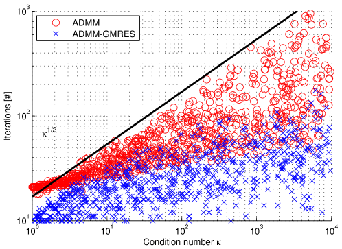
Figure 5. Number of iterations to solve 1000 randomly generated problems to $\epsilon=10^{-6}$ accuracy using ADMM with $\beta=\sqrt{m\ell}$ (circles) and GMRES-accelerated ADMM with randomly selected $\beta$ (crosses). The solid line is $17\sqrt{\kappa}$. Both methods converge in $O(\sqrt{\kappa})$ iterations. The problems have random dimensions $1\leq n_{x}\leq 1000$, $1\leq n_{y}\leq n_{x}$, $1\leq n_{z}\leq n_{y}$.

First, we compare the performance of ADMM and GMRES-accelerated ADMM in the solution of random problems generated via the following procedure taken from [34].

Construction 1.

Begin with nonzero positive integer parameters $n_{x}$, $n_{y}\leq n_{x}$, $n_{z}\leq n_{y}$ and positive real parameter $s$.

1. Select the orthogonal matrices $U_{A},U_{B}\in\mathbb{R}^{n_{y}\times n_{y}}$, $V_{A},U_{D}\in\mathbb{R}^{n_{x}\times n_{x}}$, $V_{B}\in\mathbb{R}^{n_{y}\times n_{z}}$ i.i.d. uniformly from their respective orthogonal groups.

2. Select the positive scalars $\sigma_{A}^{(1)},\ldots,\sigma_{A}^{(n_{y})}$, $\sigma_{B}^{(1)},\ldots,\sigma_{B}^{(n_{z})}$, and $\sigma_{D}^{(1)},\ldots,\sigma_{D}^{(n_{x})}$ i.i.d. from the log-normal distribution $\sim\mathrm{exp}(0,s^{2})$.

3. Output the matrices $A=U_{A}\mathrm{diag}(\sigma_{A}^{(1)},\ldots,\sigma_{A}^{(n_{y})})V_{A}^{T}$, $B=U_{B}\mathrm{diag}(\sigma_{B}^{(1)},\ldots,\sigma_{B}^{(n_{y})})V_{B}^{T}$, and $D=U_{D}\mathrm{diag}(\sigma_{D}^{(1)},\ldots,\sigma_{D}^{(n_{y})})U_{D}^{T}$.

The dimension parameters $n_{x}$, $n_{y}$, $n_{z}$ are uniformly sampled from $n_{x}\in\{1,\ldots,1000\}$, $n_{y}\in\{1,\ldots,n_{x}\}$, and $n_{z}\in\{1,\ldots,n_{z}\}$, and the log-standard-deviation uniformly swept within the range $s\in[0,1]$, in order to produce a range of condition numbers spanning $1\leq\kappa\leq 10^{4}$. Note that by construction, the optimal parameter choice $\sqrt{m\ell}$ has an expected value of 1.

Figure 5 plots the number of iterations to converge to $\epsilon=10^{-6}$ for each method and over each problem. We see that both ADMM and ADMM-GMRES converges in $O(\sqrt{\kappa})$ iterations, with ADMM-GMRES typically converging in slightly fewer iterations than ADMM. The difference, of course, is that the feat is achieved by ADMM-GMRES without needing to estimate the values of $m$ and $\ell$.

Note that the ADMM-GMRES curve bends downwards with increasing $\kappa$. This is an artifact of the distribution of $\beta$ becoming optimal with increasing $\kappa$. As we noted in the proof of our main results, the convergence of ADMM-GMRES is entirely driven by an indirect, rescaled quantity $\gamma=\max\{\ell/\beta,\beta/m\}$. When $\ell$ and $m$ are increased and decreased at the same uniform rate, the distribution for $\gamma$ and $\beta$ become concentrated about $\gamma=\sqrt{\kappa}$ and $\beta=\sqrt{m\ell}$ respectively. These choices of $\gamma$ and $\beta$ often allow ADMM-GMRES to converge in $O(\kappa^{\frac{1}{4}}\log\epsilon^{-1})$ iterations [34].

7.2. Interior-point Newton Direction for SDPs

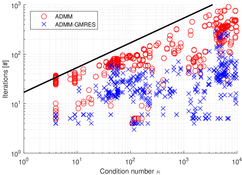
Figure 6. Number of iterations to solve 508 Newton direction subproblems with $\kappa\leq 10^{4}$ to $\epsilon=10^{-6}$ accuracy. The solid line plots $k=17\sqrt{\kappa}$.

Next, we compare the performance of ADMM and GMRES-accelerated ADMM in their ability to recompute the Newton steps as generated by SeDuMi [27] over 80 semidefinite programs (SDPs) in the SDPLIB suite [6]. The experimental set-up is similar to that described in [34]: the 80 problems from the SDPLIB suite with less than 700 constraints are pre-solved using SeDuMi, and the predictor and corrector Newton step problems at each interior-point step are exported, each of the form

(57) $$\begin{bmatrix}D&0&I\\ 0&0&B^{T}\\ I&B&0\end{bmatrix}\begin{bmatrix}\Delta x\\ \Delta z\\ \Delta y\end{bmatrix}=\begin{bmatrix}r_{x}\\ r_{z}\\ r_{y}\end{bmatrix}.$$

Clearly, this is the KKT system for the prototype ADMM problem (3) with substitutions $f(x)=\frac{1}{2}x^{T}Dx-r_{x}^{T}x$, $g(z)=-r_{z}^{T}z$, $A=I$, $c=r_{y}$, so both ADMM and ADMM-GMRES can be used to recompute the solution $[\Delta x;\Delta z;\Delta y]$. The associated matrix-vector products should be implicitly performed in order for either methods to be efficient (cf. [34, Sec. 8]), but this is an implementation detail that does not affect the iterates generated.

Figure 6 shows the number of iterations to converge to $\epsilon=10^{-6}$ over all 508 Newton direction subproblems with $\kappa\leq 10^{4}$. Again, both ADMM and ADMM-GMRES required $O(\sqrt{\kappa})$ iterations, with the latter achieving the feat without needing to estimate the values of $m$ and $\ell$. In fact, ADMM-GMRES converged in fewer iterations for all of the problems considered.

References

• [1] Z.-Z. Bai, G. H. Golub, and M. K. Ng, Hermitian and skew-hermitian splitting methods for non-hermitian positive definite linear systems, SIAM Journal on Matrix Analysis and Applications, 24 (2003), pp. 603–626.
• [2] A. Battermann and M. Heinkenschloss, Preconditioners for karush-kuhn-tucker matrices arising in the optimal control of distributed systems, in Control and Estimation of Distributed Parameter Systems, Springer, 1998, pp. 15–32.
• [3] M. Benzi and G. H. Golub, A preconditioner for generalized saddle point problems, SIAM Journal on Matrix Analysis and Applications, 26 (2004), pp. 20–41.
• [4] M. Benzi, G. H. Golub, and J. Liesen, Numerical solution of saddle point problems, Acta numerica, 14 (2005), pp. 1–137.
• [5] M. Benzi and V. Simoncini, On the eigenvalues of a class of saddle point matrices, Numerische Mathematik, 103 (2006), pp. 173–196.
• [6] B. Borchers, Sdplib 1.2, a library of semidefinite programming test problems, Optimization Methods and Software, 11 (1999), pp. 683–690.
• [7] S. Boyd, N. Parikh, E. Chu, B. Peleato, and J. Eckstein, Distributed optimization and statistical learning via the alternating direction method of multipliers, Foundations and Trends® in Machine Learning, 3 (2011), pp. 1–122.
• [8] J. H. Bramble, J. E. Pasciak, and A. T. Vassilev, Analysis of the inexact uzawa algorithm for saddle point problems, SIAM Journal on Numerical Analysis, 34 (1997), pp. 1072–1092.
• [9] P. N. Brown and Y. Saad, Convergence theory of nonlinear newton-krylov algorithms, SIAM Journal on Optimization, 4 (1994), pp. 297–330.
• [10] H. C. Elman and G. H. Golub, Inexact and preconditioned uzawa algorithms for saddle point problems, SIAM Journal on Numerical Analysis, 31 (1994), pp. 1645–1661.
• [11] H.-r. Fang and Y. Saad, Two classes of multisecant methods for nonlinear acceleration, Numerical Linear Algebra with Applications, 16 (2009), pp. 197–221.
• [12] D. G. Feingold, R. S. Varga, et al., Block diagonally dominant matrices and generalizations of the gerschgorin circle theorem, Pacific J. Math, 12 (1962), pp. 1241–1250.
• [13] G. França and J. Bento, An explicit rate bound for the over-relaxed admm, arXiv preprint arXiv:1512.02063, (2015).
• [14] E. Ghadimi, A. Teixeira, I. Shames, and M. Johansson, Optimal parameter selection for the alternating direction method of multipliers (admm): quadratic problems, Automatic Control, IEEE Transactions on, 60 (2015), pp. 644–658.
• [15] P. Giselsson and S. Boyd, Diagonal scaling in douglas-rachford splitting and admm, in Decision and Control (CDC), 2014 IEEE 53rd Annual Conference on, IEEE, 2014, pp. 5033–5039.
• [16] A. Greenbaum, Iterative methods for solving linear systems, vol. 17, Siam, 1997.
• [17] B. He, H. Yang, and S. Wang, Alternating direction method with self-adaptive penalty parameters for monotone variational inequalities, Journal of Optimization Theory and applications, 106 (2000), pp. 337–356.
• [18] Y. Nesterov, Introductory lectures on convex optimization, vol. 87, Springer Science & Business Media, 2004.
• [19] R. Nishihara, L. Lessard, B. Recht, A. Packard, and M. I. Jordan, A general analysis of the convergence of admm, arXiv preprint arXiv:1502.02009, (2015).
• [20] A. R. Oliveira and D. C. Sorensen, A new class of preconditioners for large-scale linear systems from interior point methods for linear programming, Linear Algebra and its applications, 394 (2005), pp. 1–24.
• [21] T. J. Rivlin, The Chebyshev Polynomials: From Approximation Theory to Algebra and Number Theory, John Wiley & Sons, 1974.
• [22] Y. Saad, A flexible inner-outer preconditioned gmres algorithm, SIAM Journal on Scientific Computing, 14 (1993), pp. 461–469.
• [23] Y. Saad, Iterative methods for sparse linear systems, Siam, 2003.
• [24] Y. Saad and M. H. Schultz, Gmres: A generalized minimal residual algorithm for solving nonsymmetric linear systems, SIAM Journal on scientific and statistical computing, 7 (1986), pp. 856–869.
• [25] D. A. Spielman and S.-H. Teng, Nearly linear time algorithms for preconditioning and solving symmetric, diagonally dominant linear systems, SIAM Journal on Matrix Analysis and Applications, 35 (2014), pp. 835–885.
• [26] K. Stüben, A review of algebraic multigrid, Journal of Computational and Applied Mathematics, 128 (2001), pp. 281–309.
• [27] J. F. Sturm, Using sedumi 1.02, a matlab toolbox for optimization over symmetric cones, Optimization methods and software, 11 (1999), pp. 625–653.
• [28] K.-C. Toh, Solving large scale semidefinite programs via an iterative solver on the augmented systems, SIAM Journal on Optimization, 14 (2004), pp. 670–698.
• [29] U. Trottenberg, C. W. Oosterlee, and A. Schuller, Multigrid, Academic press, 2000.
• [30] R. J. Vanderbei, Symmetric quasidefinite matrices, SIAM Journal on Optimization, 5 (1995), pp. 100–113.
• [31] R. J. Vanderbei and T. J. Carpenter, Symmetric indefinite systems for interior point methods, Mathematical Programming, 58 (1993), pp. 1–32.
• [32] N. K. Vishnoi, Laplacian solvers and their algorithmic applications, Theoretical Computer Science, 8 (2012), pp. 1–141.
• [33] S. Wang and L. Liao, Decomposition method with a variable parameter for a class of monotone variational inequality problems, Journal of optimization theory and applications, 109 (2001), pp. 415–429.
• [34] R. Y. Zhang and J. K. White, On the convergence of GMRES-accelerated ADMM in $O(\kappa^{1/4}\log\epsilon^{-1})$ iterations for quadratic objectives, arXiv preprint arXiv:1601.06200v3, (2016).