Parallel Ordered Sets Using Join

Abstract

Ordered sets (and maps when data is associated with each key) are one of the most important and useful data types. The set-set functions union, intersection and difference are particularly useful in certain applications. Brown and Tarjan first described an algorithm for these functions, based on 2-3 trees, that meet the optimal $\Theta\mathopen{}\mathclose{{}\left({m\log\mathopen{}\mathclose{{}\left(\frac{n}{m}+1}\right)}}\right)$ time bounds in the comparison model ($n$ and $m\leq n$ are the input sizes). Later Adams showed very elegant algorithms for the functions, and others, based on weight-balanced trees. They only require a single function that is specific to the balancing scheme—a function that joins two balanced trees—and hence can be applied to other balancing schemes. Furthermore the algorithms are naturally parallel. However, in the twenty-four years since, no one has shown that the algorithms are work efficient (or optimal), sequential or parallel, and even for the original weight-balanced trees.

In this paper we show that Adams’ algorithms are both work efficient and highly parallel (polylog depth) across four different balancing schemes—AVL trees, red-black trees, weight balanced trees and treaps. To do this we need careful, but simple, algorithms for Join that maintain certain invariants, and our proof is (mostly) generic across the schemes.

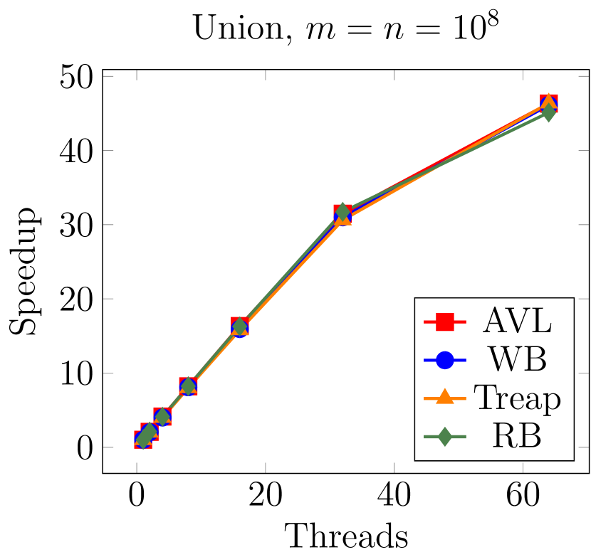
To understand how the algorithms perform in practice we have also implemented them (all code except Join is generic across the balancing schemes). Interestingly the implementations on all four balancing schemes and three set functions perform similarly in time and speedup (more than 45x on 64 cores). We also compare the performance of our implementation to other existing libraries and algorithms including the standard template library (STL) implementation of red-black trees, the multicore standard template library (MCSTL), and a recent parallel implementation based on weight-balanced trees. Our implementations are not as fast as the best of these on fully overlapping keys (but comparable), but better than all on keys with a skewed overlap (two Gaussians with different means).

1 Introduction

Ordered sets and ordered maps (sets with data associated with each key) are two of the most important data types used in modern programming. Most programming languages either have them built in as basic types (e.g. python) or supply them as standard libraries (C++, C# Java, Scala, Haskell, ML). These implementations are based on some form of balanced tree (or tree-like) data structure and, at minimum, support lookup, insertion, and deletion in logarithmic time. Most also support set-set functions such as union, intersection, and difference. These functions are particularly useful when using parallel machines since they can support parallel bulk updates. In this paper we are interested in simple and efficient parallel algorithms for such set-set functions.

The lower bound for comparison-based algorithms for union, intersection and difference for inputs of size $n$ and $m\leq n$ and output an ordered structure is $\log_{2}{m+n\choose n}=\Theta\mathopen{}\mathclose{{}\left({m\log\mathopen{}\mathclose{{}\left(\frac{n}{m}+1}\right)}}\right)$. Brown and Tarjan first described a sequential algorithm for merging that asymptotically match these bounds [11]. It can be adapted for union, intersection and difference with the same bounds. The bound is interesting since it shows that implementing insertion with union, or deletion with difference, is asymptotically efficient ($O(\log n)$ time), as is taking the union of two equal sized sets ($O(n)$ time). However, the Brown and Tarjan algorithm is complicated, and completely sequential.

⬇

insert$(T,k)$ $=$

$(T_{L},m,T_{R})$ $=$ split$(T,k)$;

join$(T_{L},k,T_{R})$

delete$(T,k)$ $=$

$(T_{L},m,T_{R})$ $=$ split$(T,k)$;

join2$(T_{L},T_{R})$

split$(T,k)$ $=$

if $T$ $=$ Leaf then $($Leaf,false,Leaf$)$

else $(L,m,R)$ $=$ expose$(T)$;

if $k=m$ then $($$L$,true,$R$$)$

else if $k<m$ then

$(L_{L},b,L_{R})$ $=$ split$(L,k)$;

$($$L_{L}$,$b$,join$(L_{R},m,R)$$)$

else $(R_{L},b,R_{R})$ $=$ split$(R,k)$;

$($join$(L,m,R_{L}),b,R_{R})$

splitLast$($$T$$)$ $=$

$(L,k,R)$ $=$ expose$(T)$;

if $R$ $=$ Leaf then $($$L,k$$)$

else $(T^{\prime},k^{\prime})$ $=$ splitLast$($$R$$)$;

$($join$($$L,k,T^{\prime}$$)$,$k^{\prime}$$)$

join2$($$T_{L}$,$T_{R}$$)$ $=$

if $T_{L}$ $=$ Leaf then $T_{R}$

else $(T_{L}^{\prime},k)$ $=$ splitLast$($$T_{L}$$)$;

join$($$T_{L}^{\prime},k,T_{R}$$)$

⬇

union$($$T_{1}$,$T_{2}$$)$ $=$

if $T_{1}$ $=$ Leaf then $T_{2}$

else if $T_{2}$ $=$ Leaf then $T_{1}$

else $($$L_{2}$,$k_{2}$,$R_{2}$$)$ $=$ expose$($$T_{2}$$)$;

$($$L_{1}$,$b$,$R_{1}$$)$ $=$ split$($$T_{1}$,$k_{2}$$)$;

$T_{L}$ $=$ union$($$L_{1}$,$L_{2}$$)$ $\|$ $T_{R}$ $=$ union$($$R_{1}$,$R_{2}$$)$;

join$($$T_{L}$,$k_{2}$,$T_{R}$$)$

intersect$($$T_{1}$,$T_{2}$$)$ $=$

if $T_{1}$ $=$ Leaf then Leaf

else if $T_{2}$ $=$ Leaf then Leaf

else $($$L_{2}$,$k_{2}$,$R_{2}$$)$ $=$ expose$($$T_{2}$$)$;

$($$L_{1}$,$b$,$R_{1}$$)$ $=$ split$($$T_{1}$,$k_{2}$$)$;

$T_{L}$ $=$ intersect$($$L_{1}$,$L_{2}$$)$ $\|$ $T_{R}$ $=$ intersect$($$R_{1}$,$R_{2}$$)$;

if $b$ $=$ true then join$($$T_{L}$,$k_{2}$,$T_{R}$$)$

else join2$($$T_{L}$,$T_{R}$$)$

difference$($$T_{1}$,$T_{2}$$)$ $=$

if $T_{1}$ $=$ Leaf then Leaf

else if $T_{2}$ $=$ Leaf then $T_{1}$

else $($$L_{2}$,$k_{2}$,$R_{2}$$)$ $=$ expose$($$T_{2}$$)$;

$($$L_{1}$,$b$,$R_{1}$$)$ $=$ split$($$T_{1}$,$k_{2}$$)$;

$T_{L}$ $=$ difference$($$L_{1}$,$L_{2}$$)$ $\|$ $T_{R}$ $=$ difference$($$R_{1}$,$R_{2}$$)$;

join2$($$T_{L}$,$T_{R}$$)$

Figure 1: Implementing Union, Intersect, Difference, Insert, Delete, Split, and Join2 with just Join. Expose returns the left tree, key, and right tree of a node. The $||$ notation indicates the recursive calls can run in parallel. These are slight variants of the algorithms described by Adams [1], although he did not consider parallelism.

Adams later described very elegant algorithms for union, intersection, and difference, as well as other functions using weight-balanced trees, based on a single function, Join [1, 2] (see Figure 1). The algorithms are naturally parallel. The Join$(L,k,R)$ function takes a key $k$ and two ordered sets $L$ and $R$ such that $L<k<R$ and returns the union of the keys [28, 26]. Join can be used to implement Join2$(L,R)$, which does not take the key in the middle, and Split$(T,k)$, which splits a tree at a key $k$ returning the two pieces and a flag indicating if $k$ is in $T$ (See Section 4). With these three functions, union, intersection, and difference (as well as insertion, deletion and other functions) are almost trivial. Because of this at least three libraries use Adams’ algorithms for their implementation of ordered sets and tables (Haskell [19] and MIT/GNU Scheme, and SML).

Join can be implemented on a variety of different balanced tree schemes. Sleator and Tarjan describe an algorithm for Join based on splay trees which runs in amortized logarithmic time [26]. Tarjan describes a version for red-black tree that runs in worst case logarithmic time [28]. Adams describes version based on weight-balanced trees [1]. Adams’ algorithms were proposed in an international competition for the Standard ML community, which is about implementations on “set of integers”. Prizes were awarded in two categories: fastest algorithm, and most elegant yet still efficient program. Adams won the elegance award, while his algorithm is as fast as the fastest program for very large sets, and was faster for smaller sets. Adams’ algorithms actually show that in principle all balance criteria for search trees can be captured by a single function Join, although he only considered weight-balanced trees.

Surprisingly, however, there have been almost no results on bounding the work (time) of Adams’ algorithms, in general nor on specific trees. Adams informally argues that his algorithms take $O(n+m)$ work for weight-balanced tree, but that is a very loose bound. Blelloch and Miller later show that similar algorithms for treaps [6], are optimal for work (i.e. $\Theta\mathopen{}\mathclose{{}\left({m\log\mathopen{}\mathclose{{}\left(\frac{n}{m}+1}\right)}}\right)$), and also parallel. Their algorithms, however, are specific for treaps. The problem with bounding the work of Adams’ algorithms, is that just bounding the time of Split, Join and Join2 with logarithmic costs is not sufficient. One needs additional properties of the trees.

The contribution of this paper is to give first work-optimal bounds for Adams’ algorithms. We do this not only for the weight-balanced trees. we bound the work and depth of Adams’ algorithms (union, intersection and difference) for four different balancing shemes: AVL trees, red-black trees, weight-balanced trees and treaps. We analyze exactly the algorithms in Figure 1, and the bounds hold when either input tree is larger. We show that with appropriate (and simple) implementations of Join for each of the four balancing schemes, we achieve asymptotically optimal bounds on work. Furthermore the algorithms have $O(\log n\log m)$ depth, and hence are highly parallel. To prove the bounds on work we show that our implementations of Join satisfy certain conditions based on a rank we define for each tree type. In particular the cost of Join must be proportional to the difference in ranks of two trees, and the rank of the result of a join must be at most one more than the maximum rank of the two arguments.

In addition to the theoretical analysis of the algorithms, we implemented parallel versions of all of the algorithms on all four tree types and describe a set of experiments. Our implementation is generic in the sense that we use common code for the algorithms in Figure 1, and only wrote specialized code for each tree type for the Join function. Our implementations of Join are as described in this paper. We compare performance across a variety of parameters. We compare across the tree types, and interestingly all four balance criteria have very similar performance. We measure the speedup on up to 64 cores and achieve close to a 46-fold speedup. We compare to other implementations, including the set implementation in the C++ Standard Template library (STL) for sequential performance, and parallel weight-balanced B-trees (WBB-trees) [12] and the multi-core standard template library (MCSTL) [13] for parallel performance. We also compare for different data distributions. The conclusion from the experiments is that although not always as fast as (WBB-trees) [12] on uniform distributions, the generic code is quite competitive, and on keys with a skewed overlap (two Gaussians with different means), our implementation is much better than all the other baselines.

Related Work

Parallel set operations on two ordered sets have been well-studied, but each previous algorithm only works on one type of balance tree. Paul, Vishkin, and Wagener studied bulk insertion and deletion on 2-3 trees in the PRAM model [24]. Park and Park showed similar results for red-black trees [23]. These algorithms are not based on Join. Katajainen [16] claimed an algorithm with $O\mathopen{}\mathclose{{}\left(m\log(\frac{n}{m}+1)}\right)$ work and $O(\log n)$ depth using 2-3 tree, but was shown to contain some bugs so the bounds do not hold [6]. Akhremtsev and Sanders [4] (unpublished) recently fixed that and proposed an algorithm based on $(a,b)$-trees with optimal work and $O(\log n)$ depth. Their algorithm only works for $(a,b)$-trees, and they only gave algorithms on Union. Besides, our algorithm is much simpler and easy to be implemented than theirs. Blelloch and Miller showed a similar algorithm as Adams’ (as well as ours) on treaps with optimal work and $O(\log n)$ depth on a EREW PRAM with scan operation using pipelines (implying $O(\log n\log m)$ depth on a plain EREW PRAM, and $O(\log^{*}m\log n)$ depth on a plain CRCW PRAM). The pipelining is quite complicated. Our focus in this paper is in showing that very simple algorithm are work efficient and have polylogarithmic depth, and less with optimizing the depth.

Many researchers have considered concurrent implementations of balanced search trees (e.g., [17, 18, 10, 21]). None of these is work efficient for Union since it is necessary to insert one tree into the other taking work at least $O(m\log n)$. Furthermore the overhead of concurrency is likely to be very high.

2 Preliminaries

A binary tree is either a Leaf, or a node consisting of a left binary tree $T_{L}$, a value (or key) $v$, and a right binary tree $T_{R}$, and denoted Node$(T_{L},v,T_{R})$. The size of a binary tree, or $|T|$, is $0$ for a Leaf and $|T_{L}|+|T_{R}|+1$ for a Node$(T_{L},v,T_{R})$. The weight of a binary tree, or $w(T)$, is one more than its size (i.e., the number of leaves in the tree). The height of a binary tree, or $h(T)$, is $0$ for a Leaf, and $\max(h(T_{L}),h(T_{R}))+1$ for a Node$(T_{L},v,T_{R})$. Parent, child, ancestor and descendant are defined as usual (ancestor and descendant are inclusive of the node itself). The left spine of a binary tree is the path of nodes from the root to a leaf always following the left tree, and the right spine the path to a leaf following the right tree. The in-order values of a binary tree is the sequence of values returned by an in-order traversal of the tree.

A balancing scheme for binary trees is an invariant (or set of invariants) that is true for every node of a tree, and is for the purpose of keeping the tree nearly balanced. In this paper we consider four balancing schemes that ensure the height of every tree of size $n$ is bounded by $O(\log n)$. For each balancing scheme we define the rank of a tree, or $r(T)$.

AVL trees [3] have the invariant that for every $\mbox{\tt Node}(T_{L},v,T_{R})$, the height of $T_{L}$ and $T_{R}$ differ by at most one. This property implies that any AVL tree of size $n$ has height at most $\log_{\phi}(n+1)$, where $\phi=\frac{1+\sqrt{5}}{2}$ is the golden ratio. For AVL trees $r(T)=h(T)-1$.

Red-black (RB) trees [5] associate a color with every node and maintain two invariants: (the red rule) no red node has a red child, and (the black rule) the number of black nodes on every path from the root down to a leaf is equal. Unlike some other presentations, we do not require that the root of a tree is black. Our proof of the work bounds requires allowing a red root. We define the black height of a node $T$, denoted $\hat{h}(T)$ to be the number of black nodes on a downward path from the node to a leaf (inclusive of the node). Any RB tree of size $n$ has height at most $2\log_{2}(n+1)$. In RB trees $r(T)=2(\hat{h}(T)-1)$ if $T$ is black and $r(T)=2\hat{h}(T)-1$ if $T$ is red.

Weight-balanced (WB) trees with parameter $\alpha$ (also called BB$[\alpha]$ trees) [22] maintain for every $T=\mbox{\tt Node}(T_{L},v,T_{R})$ the invariant $\alpha\leq\frac{w(T_{L})}{w(T)}\leq 1-\alpha$. We say two weight-balanced trees $T_{1}$ and $T_{2}$ have like weights if $\mbox{\tt Node}(T_{1},v,T_{2})$ is weight balanced. Any $\alpha$ weight-balanced tree of size $n$ has height at most $\log_{\frac{1}{1-\alpha}}n$. For $\frac{2}{11}<\alpha\leq 1-\frac{1}{\sqrt{2}}$ insertion and deletion can be implemented on weight balanced trees using just single and double rotations [22, 7]. We require the same condition for our implementation of Join, and in particular use $\alpha=0.29$ in experiments. For WB trees $r(T)=\lceil\log_{2}(w(T))\rceil-1$.

Treaps [25] associate a uniformly random priority with every node and maintain the invariant that the priority at each node is no greater than the priority of its two children. Any treap of size $n$ has height $O(\log n)$ with high probability (w.h.p). For treaps $r(T)=\lceil\log_{2}(w(T))\rceil-1$.

For all the four balancing schemes $r(T)=\Theta(\log(|T|+1))$. The notation we use for binary trees is summarized in Table 1.

A Binary Search Tree (BST) is a binary tree in which each value is a key taken from a total order, and for which the in-order values are sorted. A balanced BST is a BST maintained with a balancing scheme, and is an efficient way to represent ordered sets.

Our algorithms are based on nested parallelism with nested fork-join constructs and no other synchronization or communication among parallel tasks. All algorithms are deterministic. We use work ($W$) and span ($S$) to analyze asymptotic costs, where the work is the total number of operations and span is the critical path. We use the simple composition rules $W(e_{1}~{}||~{}e_{2})=W(e_{1})+W(e_{2})+1$ and $S(e_{1}~{}||~{}e_{2})=\max(S(e_{1}),S(e_{2}))+1$. For sequential computation both work and span compose with addition. Any computation with $W$ work and $S$ span will run in time $T<\frac{W}{P}+S$ assuming a PRAM (random access shared memory) with $P$ processors and a greedy scheduler [9, 8].

Notation	Description
$|T|$	The size of tree $T$
$h(T)$	The height of tree $T$
$\hat{h}(T)$	The black height of an RB tree $T$
$r(T)$	The rank of tree $T$
$w(T)$	The weight of tree $T$ (i.e, $|T|+1$)
$p(T)$	The parent of node $T$
$k(T)$	The value (or key) of node $T$
$L(T)$	The left child of node $T$
$R(T)$	The right child of node $T$
expose$(T)$	$(L(T),k(T),R(T))$

Table 1: Summary of notation.

3 The JOIN Function

Here we describe algorithms for Join for the four balancing schemes we defined in Section 2. The function Join$(T_{L},k,T_{R})$ takes two binary trees $T_{L}$ and $T_{R}$, and a value $k$, and returns a new binary tree for which the in-order values are a concatenation of the in-order values of $T_{L}$, then $k$, and then the in-order values of $T_{R}$.

As mentioned in the introduction and shown in Section 4, Join fully captures what is required to rebalance a tree and can be used as the only function that knows about and maintains the balance invariants. For AVL, RB and WB trees we show that Join takes work that is proportional to the difference in rank of the two trees. For treaps the work depends on the priority of $k$. All versions of Join are sequential so the span is equal to the work. Due to space limitations, we describe the algorithms, state the theorems for all balancing schemes, but only show a proof outline for AVL trees.

⬇

1joinRight$(T_{L},k,T_{R})$ $=$

2 $(l,k^{\prime},c)$ $=$ expose$(T_{L})$;

3 if $h(c)\leq h(T_{R})+1$ then

4 $T^{\prime}=\mbox{\tt Node}(c,k,T_{R})$;

5 if $h(T^{\prime})\leq h(l)+1$ then $\mbox{\tt Node}(l,k^{\prime},T^{\prime})$

6 else rotateLeft$($Node$($$l,k^{\prime},$ rotateRight$(T^{\prime})$$)$$)$

7 else

8 $T^{\prime}$ $=$ joinRight$(c,k,T_{R})$;

9 $T^{\prime\prime}$ $=$ $\mbox{\tt Node}(l,k^{\prime},T^{\prime})$;

10 if $h(T^{\prime})\leq h(l)+1$ then $T^{\prime\prime}$

11 else rotateLeft$(T^{\prime\prime})$

12join$(T_{L},k,T_{R})$ $=$

13 if $h(T_{L})>h(T_{R})+1$ then joinRight$(T_{L},k,T_{R})$

14 else if $h(T_{R})>h(T_{L})+1$ then joinLeft$(T_{L},k,T_{R})$

15 else $\mbox{\tt Node}(T_{L},k,T_{R})$

Figure 2: AVL Join algorithm.

⬇

1joinRightRB$(T_{L},k,T_{R})$ $=$

2 if $($$r(T_{L})=\lfloor r(T_{R})/2\rfloor\times 2$$)$ then

3 $\mbox{\tt Node}(T_{L},\mathopen{}\mathclose{{}\left<k,\texttt{red}}\right>,T_{R})$;

4 else

5 $(L^{\prime},\mathopen{}\mathclose{{}\left<k^{\prime},c^{\prime}}\right>,R^{\prime})$$=$expose$($$T_{L}$$)$;

6 $T^{\prime}$ $=$ $\mbox{\tt Node}(L^{\prime},\mathopen{}\mathclose{{}\left<k^{\prime},c^{\prime}}\right>$,joinRightRB$(R^{\prime},k,T_{R}))$;

7 if $($$c^{\prime}$$=$black$)$ and $($$c(R(T^{\prime}))=c(R(R(T^{\prime})))$$=$red$)$ then

8 $c(R(R(T^{\prime})))$$=$black;

9 $T^{\prime\prime}$$=$rotateLeft$(T^{\prime})$

10 else $T^{\prime\prime}$

11joinRB$(T_{L},k,T_{R})$ $=$

12 if $\lfloor r(T_{L})/2\rfloor>\lfloor r(T_{R})/2\rfloor$ then

13 $T^{\prime}=$joinRightRB$(T_{L},k,T_{R})$;

14 if $($$c(T^{\prime})$$=$red$)$ and $($$c(R(T^{\prime}))$$=$red$)$ then

15 $\mbox{\tt Node}(L(T^{\prime}),\mathopen{}\mathclose{{}\left<k(T^{\prime}),\texttt{black}}\right>,R(T^{\prime}))$

16 else $T^{\prime}$

17 else if $\lfloor r(T_{R})/2\rfloor>\lfloor r(T_{L})/2\rfloor$ then

18 $T^{\prime}=$joinLeftRB$(T_{L},k,T_{R})$;

19 if $($$c(T^{\prime})$$=$red$)$ and $($$c(L(T^{\prime}))$$=$red$)$ then

20 $\mbox{\tt Node}(L(T^{\prime}),\mathopen{}\mathclose{{}\left<k(T^{\prime}),\texttt{black}}\right>,R(T^{\prime}))$

21 else $T^{\prime}$

22 else if $($$c(T_{L})$$=$black$)$ and $($$c(T_{R})$$=$black$)$ then

23 $\mbox{\tt Node}(T_{L},\mathopen{}\mathclose{{}\left<k,\texttt{red}}\right>,T_{R})$

24 else $\mbox{\tt Node}(T_{L},\mathopen{}\mathclose{{}\left<k,\texttt{black}}\right>,T_{R})$

Figure 3: RB Join algorithm.

⬇

1joinRightWB$(T_{L},k,T_{R})$ $=$

2 $($$l,k^{\prime},c$$)$$=$expose$($$T_{L}$$)$;

3 if $($balance$($$|T_{L}|,|T_{R}|$$)$ then $\mbox{\tt Node}(T_{L},k,T_{R}))$;

4 else

5 $T^{\prime}$ $=$ joinRightWB$(c,k,T_{R})$;

6 $(l_{1},k_{1},r_{1})$ $=$ expose$(T^{\prime})$;

7 if like$(|l|,|T^{\prime}|)$ then Node$($$l,k^{\prime},T^{\prime}$$)$

8 else if $($like$(|l|,|l_{1}|)$$)$ and $($like$(|l|+|l_{1}|,r_{1})$$)$ then

9 rotateLeft$($Node$($$l,k^{\prime},T^{\prime}$$)$$)$

10 else rotateLeft$($Node$($$l,k^{\prime}$,rotateRight$(T^{\prime})$$)$$)$

11joinWB$(T_{L},k,T_{R})$ $=$

12 if heavy$($$T_{L},T_{R}$$)$ then joinRightWB$(T_{L},k,T_{R})$

13 else if heavy$($$T_{R},T_{L}$$)$ then joinLeftWB$(T_{L},k,T_{R})$

14 else $\mbox{\tt Node}(T_{L},k,T_{R})$

Figure 4: WB Join algorithm.

⬇

1joinTreap$(T_{L},k,T_{R})$ $=$

2 if prior$($$k,k_{1}$$)$ and prior$($$k,k_{2}$$)$ then $\mbox{\tt Node}(T_{L},k,T_{R})$

3 else $($$l_{1},k_{1},r_{1}$$)$$=$expose$($$T_{L}$$)$;

4 $($$l_{2},k_{2},r_{2}$$)$$=$expose$($$T_{R}$$)$;

5 if prior$($$k_{1},k_{2}$$)$ then

6 Node$($$l_{1},k_{1}$,joinTreap$(r_{1},k,T_{R})$$)$

7 else Node$($joinTreap$($$T_{L},k,l_{2}$$)$,$k_{2},r_{2}$$)$

Figure 5: Treap Join algorithm.

AVL trees. Pseudocode for AVL Join is given in Figure 2 and illustrated in Figure 6. Every node stores its own height so that $h(\cdot)$ takes constant time. If the two trees $T_{L}$ and $T_{R}$ differ by height at most one, Join can simply create a new Node$(T_{L},k,T_{R})$. However if they differ by more than one then rebalancing is required. Suppose that $h(T_{L})>h(T_{R})+1$ (the other case is symmetric). The idea is to follow the right spine of $T_{L}$ until a node $c$ for which $h(c)\leq h(T_{R})+1$ is found (line 3). At this point a new $\mbox{\tt Node}(c,k,T_{R})$ is created to replace $c$ (line 4). Since either $h(c)=h(T_{R})$ or $h(c)=h(T_{R})+1$, the new node satisfies the AVL invariant, and its height is one greater than $c$. The increase in height can increase the height of its ancestors, possibly invalidating the AVL invariant of those nodes. This can be fixed either with a double rotation if invalid at the parent (line 6) or a single left rotation if invalid higher in the tree (line 11), in both cases restoring the height for any further ancestor nodes. The algorithm will therefore require at most two rotations.

Figure 6: An example for Join on AVL trees ($h(T_{L})>h(T_{R})+1$). We first follow the right spine of $T_{L}$ until a subtree of height at most $h(T_{r})+1$ is found (i.e., $T_{2}$ rooted at $c$). Then a new Node$(c,k,T_{R})$ is created, replacing $c$ (Step 1). If $h(T_{1})=h$ and $h(T_{2})=h+1$, the node $p$ will no longer satisfy the AVL invariant. A double rotation (Step 2) restores both balance and its original height.

Lemma 1.

For two AVL trees $T_{L}$ and $T_{R}$, the AVL Join algorithm works correctly, runs with $O(|h(T_{L})-h(T_{R})|)$ work, and returns a tree satisfying the AVL invariant with height at most $1+\max(h(T_{L}),h(T_{R}))$.

Proof outline. Since the algorithm only visits nodes on the path from the root to $c$, and only requires at most two rotations, it does work proportional to the path length. The path length is no more than the difference in height of the two trees since the height of each consecutive node along the right spine of $T_{L}$ differs by at least one. Along with the case when $h(T_{R})>h(T_{L})+1$, which is symmetric, this gives the stated work bounds. The resulting tree satisfies the AVL invariants since rotations are used to restore the invariant (details left out). The height of any node can increase by at most one, so the height of the whole tree can increase by at most one. ∎

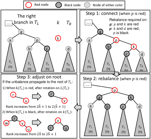
Red-black Trees. Tarjan describes how to implement the Join function for red-black trees  [28]. Here we describe a variant that does not assume the roots are black (this is to bound the increase in rank by Union). The pseudocode is given in Figure 3. We store at every node its black height $\hat{h}(\cdot)$. The first case is when $\hat{h}(T_{R})=\hat{h}(T_{L})$. Then if both $k(T_{R})$ and $k(T_{L})$ are black, we create red $\mbox{\tt Node}(T_{L},k,T_{R})$, otherwise we create black $\mbox{\tt Node}(T_{L},k,T_{R})$. The second case is when $\hat{h}(T_{R})<\hat{h}(T_{L})=\hat{h}$ (the third case is symmetric). Similarly to AVL trees, Join follows the right spine of $T_{L}$ until it finds a black node $c$ for which $\hat{h}(c)=\hat{h}(T_{R})$. It then creates a new red Node$(c,k,T_{R})$ to replace $c$. Since both $c$ and $T_{R}$ have the same height, the only invariant that can be violated is the red rule on the root of $T_{R}$, the new node, and its parent, which can all be red. In the worst case we may have three red nodes in a row. This is fixed by a single left rotation: if a black node $v$ has $R(v)$ and $R(R(v))$ both red, we turn $R(R(v))$ black and perform a single left rotation on $v$. The update is illustrated in Figure 7. The rotation, however can again violate the red rule between the root of the rotated tree and its parent, requiring another rotation. The double-red issue might proceed up to the root of $T_{L}$. If the original root of $T_{L}$ is red, the algorithm may end up with a red root with a red child, in which case the root will be turned black, turning $T_{L}$ rank from $2\hat{h}-1$ to $2\hat{h}$. If the original root of $T_{L}$ is black, the algorithm may end up with a red root with two black children, turning the rank of $T_{L}$ from $2\hat{h}-2$ to $2\hat{h}-1$. In both cases the rank of the result tree is at most $1+r(T_{L})$.

Lemma 2.

For two RB trees $T_{L}$ and $T_{R}$, the RB Join algorithm works correctly, runs with $O(|r(T_{L})-r(T_{R})|)$ work, and returns a tree satisfying the red-black invariants and with rank at most $1+\max(r(T_{L}),r(T_{R}))$.

The proof is similar as Lemma 1.

Figure 7: An example of Join on red-black trees ($\hat{h}=\hat{h}(T_{L})>\hat{h}(T_{R})$). We follow the right spine of $T_{L}$ until we find a black node with the same black height as $T_{R}$ (i.e., $c$). Then a new red Node$(c,k,T_{R})$ is created, replacing $c$ (Step 1). The only invariant that can be violated is when either $c$’s previous parent $p$ or $T_{R}$’s root $d$ is red. If so, a left rotation is performed at some black node. Step 2 shows the rebalance when $p$ is red. The black height of the rotated subtree (now rooted at $p$) is the same as before ($h+1$), but the parent of $p$ might be red, requiring another rotation. If the red-rule violation propagates to the root, the root is either colored red, or rotated left (Step 3).

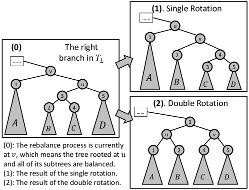
Weight Balanced Trees. We store the weight of each subtree at every node. The algorithm for joining two weight-balanced trees is similar to that of AVL trees and RB trees. The pseudocode is shown in Figure 4. The like function in the code returns true if the two input tree sizes are balanced, and false otherwise. If $T_{L}$ and $T_{R}$ have like weights the algorithm returns a new Node$(T_{L},k,T_{R})$. Suppose $|T_{R}|\leq|T_{L}|$, the algorithm follows the right branch of $T_{L}$ until it reaches a node $c$ with like weight to $T_{R}$. It then creates a new $\mbox{\tt Node}(c,k,T_{R})$ replacing $c$. The new node will have weight greater than $c$ and therefore could imbalance the weight of $c$’s ancestors. This can be fixed with a single or double rotation (as shown in Figure 8) at each node assuming $\alpha$ is within the bounds given in Section 2.

Figure 8: An illustration of single and double rotations possibly needed to rebalance weight-balanced trees. In the figure the subtree rooted at $u$ has become heavier due to joining in $T_{L}$ and its parent $v$ now violates the balance invariant.

Lemma 3.

For two $\alpha$ weight-balanced trees $T_{L}$ and $T_{R}$ and $\alpha\leq 1-\frac{1}{\sqrt{2}}\approx 0.29$, the weight-balanced Join algorithm works correctly, runs with $O(|\log(w(T_{L})/w(T_{R}))|)$ work, and returns a tree satisfying the $\alpha$ weight-balance invariant and with rank at most $1+\max(r(T_{L}),r(T_{R}))$.

The proof is shown in the Appendix.

Treaps. The treap Join algorithm (as in Figure 5) first picks the key with the highest priority among $k$, $k(T_{L})$ and $k(T_{R})$ as the root. If $k$ is the root then the we can return Node$(T_{L},k,T_{R})$. Otherwise, WLOG, assume $k(T_{L})$ has a higher priority. In this case $k(T_{L})$ will be the root of the result, $L(T_{L})$ will be the left tree, and $R(T_{L})$, $k$ and $T_{R}$ will form the right tree. Thus Join recursively calls itself on $R(T_{L})$, $k$ and $T_{R}$ and uses result as $k(T_{L})$’s right child. When $k(T_{R})$ has a higher priority the case is symmetric. The cost of Join is therefore the depth of the key $k$ in the resulting tree (each recursive call pushes it down one level). In treaps the shape of the result tree, and hence the depth of $k$, depend only on the keys and priorities and not the history. Specifically, if a key has the $t^{th}$ highest priority among the keys, then its expected depth in a treap is $O(\log t)$ (also w.h.p.). If it is the highest priority, for example, then it remains at the root.

Lemma 4.

For two treaps $T_{L}$ and $T_{R}$, if the priority of $k$ is the $t$-th highest among all keys in $T_{L}\cup\{k\}\cup T_{R}$, the treap Join algorithm works correctly, runs with $O(\log t+1)$ work in expectation and w.h.p., and returns a tree satisfying the treap invariant with rank at most $1+\max(r(T_{L}),r(T_{R}))$.

From the above lemmas we can get the following fact for Join.

Theorem 1.

For AVL, RB and WB trees Join$(T_{L},k,T_{R})$ does $O\mathopen{}\mathclose{{}\left(|r(T_{L})-r(T_{R})|}\right)$ work. For treaps Join does $O(\log t)$ work in expectation if $k$ has the $t$-th highest priority among all keys. For AVL, RB, WB trees and treaps, Join returns a tree $T$ for which the rank satisfies $\max\mathopen{}\mathclose{{}\left(r(T_{L}),r(T_{R})}\right)\leq r(T)\leq 1+\max(r(T_{L}),r(T_{R}))$.

4 Other Functions Using JOIN

In this section, we describe algorithms for various functions that use just Join. The algorithms are generic across balancing schemes. The pseudocodes for the algorithms in this section is shown in Figure 1.

Split. For a BST $T$ and key $k$, Split$(T,k)$ returns a triple $(T_{L},b,T_{R})$, where $T_{L}$ ($T_{R}$) is a tree containing all keys in $T$ that are less (larger) than $k$, and $b$ is a flag indicating whether $k\in T$. The algorithm first searches for $k$ in $T$, splitting the tree along the path into three parts: keys to the left of the path, $k$ itself (if it exists), and keys to the right. Then by applying Join, the algorithm merges all the subtrees on the left side (using keys on the path as intermediate nodes) from bottom to top to form $T_{L}$, and merges the right parts to form $T_{R}$. Figure 9 gives an example.

Figure 9: An example of Split in a BST with key $42$. We first search for $42$ in the tree and split the tree by the searching path, then use Join to combine trees on the left and on the right respectively, bottom-top.

Theorem 2.

The work of Split$(T,k)$ is $O(\log|T|)$ for all balancing schemes described in Section 3 (w.h.p. for treaps). The two resulting trees $T_{L}$ and $T_{R}$ will have rank at most $r(T)$.

Proof.

We only consider the work of joining all subtrees on the left side. The other side is symmetric. Suppose we have $l$ subtrees on the left side, denoted from bottom to top as $T_{1},T_{2},\dots T_{l}$. We have that $r(T_{1})\leq r(T_{2})\leq\dots\leq r(T_{l})$. As stated above, we consecutively join $T_{1}$ and $T_{2}$ returning $T^{\prime}_{2}$, then join $T^{\prime}_{2}$ with $T_{3}$ returning $T^{\prime}_{3}$ and so forth, until all trees are merged. The overall work of Split is the sum of the cost of $l-1$ Join functions.

For AVL trees, red-black trees and weight-balanced trees, recall Theorem 1 that we have $r(T^{\prime}_{i})\leq r(T_{i})+1$, so $r(T^{\prime}_{i})\leq r(T_{i})+1\leq r(T_{i+1})+1$. According to Theorem 1, the work of a single operation is $O(|r(T_{i+1})-r(T^{\prime}_{i})|)$. The overall complexity is $\sum_{i=1}^{l}|r(T_{i+1})-r(T^{\prime}_{i})|\leq\sum_{i=1}^{l}r(T_{i+1})-r(T^{\prime}_{i})+2=O(r(T))=O(\log|T|)$.

For treaps, each Join uses the key with the highest priority since the key is always on a upper level. Hence by Lemma 4, the complexity of each Join is $O(1)$ and the work of split is at most $O(\log|T|)$ w.h.p.

Also notice that when getting the final result $T_{L}$ and $T_{R}$, the last step is a Join on two trees, the larger one of which is a subtree of the original $T$. Thus the rank of the two trees to be joined is of rank at most $r(T)-1$, according to Theorem 1 we have $r(T_{L})$ and $r(T_{R})$ at most $r(T)$. ∎

Join2. Join2$(T_{L},T_{R})$ returns a binary tree for which the in-order values is the concatenation of the in-order values of the binary trees $T_{L}$ and $T_{R}$ (the same as Join but without the middle key). For BSTs, all keys in $T_{L}$ have to be less than keys in $T_{R}$. Join2 first finds the last element $k$ (by following the right spine) in $T_{L}$ and on the way back to root, joins the subtrees along the path, which is similar to Split $T_{L}$ by $k$. We denote the result of dropping $k$ in $T_{L}$ as $T_{L}^{\prime}$. Then Join($T_{L}^{\prime},k,T_{R}$) is the result of Join2. Unlike Join, the work of Join2 is proportional to the rank of both trees since both Split and Join take at most logarithmic work.

Theorem 3.

The work of Join2$(T_{L},T_{R})$ is $O(r(T_{L})+r(T_{R}))$ for all balancing schemes described in Section 3 (bounds are w.h.p for treaps).

Union, Intersect and Difference. Union$(T_{1},T_{2})$ takes two BSTs and returns a BST that contains the union of all keys. The algorithm uses a classic divide-and-conquer strategy, which is parallel. At each level of recursion, $T_{1}$ is split by $k(T_{2})$, breaking $T_{1}$ into three parts: one with all keys smaller than $k(T_{2})$ (denoted as $L_{1}$), one in the middle either of only one key equal to $k(T_{2})$ (when $k(T_{2})\in T_{1}$) or empty (when $k(T_{2})\notin T_{1}$), the third one with all keys larger than $k(T_{2})$ (denoted as $R_{1}$). Then two recursive calls to Union are made in parallel. One unions $L(T_{2})$ with $L_{1}$, returning $T_{L}$, and the other one unions $R(T_{2})$ with $R_{1}$, returning $T_{R}$. Finally the algorithm returns Join$(T_{L},k(T_{2}),T_{R})$, which is valid since $k(T_{2})$ is greater than all keys in $T_{L}$ are less than all keys in $T_{R}$.

The functions Intersect$(T_{1},T_{2})$ and Difference$(T_{1},T_{2})$ take the intersection and difference of the keys in their sets, respectively. The algorithms are similar to Union in that they use one tree to split the other. However, the method for joining is different. For Intersect, Join2 is used instead of Join if the root of the first is not found in the second. For Difference, Join2 is used anyway because $k(T_{2})$ should be excluded in the result tree. The base cases are also different in the obvious way.

Theorem 4 (Main Theorem).

For all the four balance schemes mentioned in Section 3, the work and span of the algorithm (as shown in Figure 1) of Union, Intersect or Difference on two balanced BSTs of sizes $m$ and $n$ ($n\geq m$) is $\displaystyle O\mathopen{}\mathclose{{}\left({m\log\mathopen{}\mathclose{{}\left(\frac{n}{m}+1}\right)}}\right)$ and $O(\log n\log m)$ respectively (the bound is in expectation for treaps).

A generic proof of Theorem 4 working for all the four balancing schemes will be shown in the next section.

The work bound for these algorithms is optimal in the comparison-based model. In particular considering all possible interleavings, the minimum number of comparisons required to distinguish them is $\log{m+n\choose n}=\Theta\mathopen{}\mathclose{{}\left({m\log\mathopen{}\mathclose{{}\left(\frac{n}{m}+1}\right)}}\right)$ [15].

Other Functions. Many other functions can be implemented with Join. Pseudocode for Insert and Delete was given in Figure 1. For a tree of size $n$ they both take $O(\log n)$ work.

5 The Proof of the Main Theorem

In this section we prove Theorem 4, for all the four balance schemes (AVL trees, RB trees, WB trees and treaps) and all three set algorithms (Union, Intersect, Difference) from Figure 1. For this purpose we make two observations. The first is that all the work for the algorithms can be accounted for within a constant factor by considering just the work done by the Splits and the Joins (or Join2s), which we refer to as split work and join work, respectively. This is because the work done between each split and join is constant. The second observation is that the split work is identical among the three set algorithms. This is because the control flow of the three algorithms is the same on the way down the recursion when doing Splits—the algorithms only differ in what they do at the base case and on the way up the recursion when they join.

Given these two observations, we prove the bounds on work by first showing that the join work is asymptotically at most as large as the split work (by showing that this is true at every node of the recursion for all three algorithms), and then showing that the split work for Union (and hence the others) satisfies our claimed bounds.

Notation	Description
$T_{p}$	The pivot tree
$T_{d}$	The decomposed tree
$n$	$\max(|T_{p}|,|T_{d}|)$
$m$	$\min(|T_{p}|,|T_{d}|)$
$T_{p}(v),v\in T_{p}$	The subtree rooted at $v$ in $T_{p}$
$T_{d}(v),v\in T_{p}$	The tree from $T_{d}$ that $v$ splits
$s_{i}$	The number of nodes in layer $i$
$v_{kj}$	The $j$-th node on layer $k$ in $T_{p}$
$d(v)$	The number of nodes attached to a layer
	root $v$ in a treap

Table 2: Descriptions of notations used in the proof.

We start with some notation, which is summarized in Table 2. In the three algorithms the first tree ($T_{1}$) is split by the keys in the second tree ($T_{2}$). We therefore call the first tree the decomposed tree and the second the pivot tree, denoted as $T_{d}$ and $T_{p}$ respectively. The tree that is returned is denoted as $T_{r}$. Since our proof works for either tree being larger, we use $m=\min(|T_{p}|,|T_{d}|)$ and $n=\max(|T_{p}|,|T_{d}|)$. We denote the subtree rooted at $v\in T_{p}$ as $T_{p}(v)$, and the tree of keys from $T_{d}$ that $v$ splits as $T_{d}(v)$ (i.e., Split$(v,T_{d}(v))$ is called at some point in the algorithm). For $v\in T_{p}$, we refer to $|T_{d}(v)|$ as its splitting size.

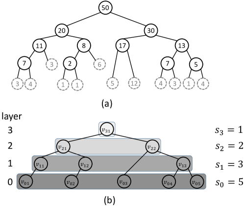
Figure 10 (a) illustrates the pivot tree with the splitting size annotated on each node. Since Split has logarithmic work, we have,

$$\mbox{split work }=O\mathopen{}\mathclose{{}\left(\sum_{v\in T_{p}}(\log|T_{d}(v)|+1)}\right),$$

which we analyze in Theorem 6. We first, however, show that the join work is bounded by the split work. We use the following Lemma, which is proven in the appendix.

Lemma 5.

For $T_{r}=$Union$(T_{p},T_{d})$ on AVL, RB or WB trees, if $r(T_{p})>r(T_{d})$ then $r(T_{r})\leq r(T_{p})+r(T_{d})$.

Theorem 5.

For each function call to Union, Intersect or Difference on trees $T_{p}(v)$ and $T_{d}(v)$, the work to do the Join (or Join2) is asymptotically no more than the work to do the Split.

Proof.

For Intersect or Difference, the cost of Join (or Join2) is $O(\log(|T_{r}|+1))$. Notice that Difference returns the keys in $T_{d}\backslash T_{p}$. Thus for both Intersect and Difference we have $T_{r}\subseteq T_{d}$. The join work is $O(\log(|T_{r}|+1))$, which is no more than $O(\log(|T_{d}|+1))$ (the split work).

For Union, if $r(T_{p})\leq r(T_{d})$, the Join will cost $O(r(T_{d}))$, which is no more than the split work.

Consider $r(T_{p})>r(T_{d})$ for AVL, RB or WB trees. The rank of $L(T_{p})$ and $R(T_{p})$, which are used in the recursive calls, are at least $r(T_{p})-1$. Using Lemma 5, the rank of the two trees returned by the two recursive calls will be at least $(r(T_{p})-1)$ and at most $(r(T_{p})+r(T_{d}))$, and differ by at most $O(r(T_{d}))=O(\log|T_{d}|+1)$. Thus the join cost is $O(\log|T_{d}|+1)$, which is no more than the split work.

Consider $r(T_{p})>r(T_{d})$ for treaps. If $r(T_{p})>r(T_{d})$, then $|T_{p}|\geq|T_{d}|$. The root of $T_{p}$ has the highest priority among all $|T_{p}|$ keys, so on expectation it takes at most the $\frac{|T_{p}|+|T_{d}|}{|T_{p}|}\leq 2$-th place among all the $|T_{d}|+|T_{p}|$ keys. From Lemma 4 we know that the cost on expectation is $\mathbb{E}[\log t]+1\leq\log\mathbb{E}[t]+1\leq\log 2+1$, which is a constant. ∎

Figure 10: An illustration of splitting tree and layers. The tree in (a) is $T_{p}$, the dashed circle are the exterior nodes. The numbers on the nodes are the sizes of the tree from $T_{d}$ to be split by this node, i.e., the “splitting size” $|T_{d}(v)|$. In (b) is an illustration of layers on an AVL tree.

This implies the total join work is asymptotically bounded by the split work.

We now analyze the split work. We do this by layering the pivot tree starting at the leaves and going to the root and such that nodes in a layer are not ancestors of each other. We define layers based on the ranks and denote the size of layer $i$ as $s_{i}$. We show that $s_{i}$ shrinks geometrically, which helps us prove our bound on the split work. For AVL and RB trees, we group the nodes with rank $i$ in layer $i$. For WB trees and treaps, we put a node $v$ in layer $i$ iff $v$ has rank $i$ and $v$’s parent has rank strictly greater than $i$. Figure 10 (b) shows an example of the layers of an AVL tree.

Definition 1.

In a BST, a set of nodes $V$ is called a disjoint set if and only if for any two nodes $v_{1},v_{2}$ in $V$, $v_{1}$ is not the ancestor of $v_{2}$.

Lemma 6.

For any disjoint set $V\subseteq T_{p}$, $\sum_{v\in V}|T_{d}(v)|\leq|T_{d}|$.

The proof of this Lemma is straightforward.

Lemma 7.

For an AVL, RB, WB tree or a treap of size $N$, each layer is a disjoint set, and $s_{i}\leq\frac{N}{c^{\lfloor i/2\rfloor}}$ holds for some constant $c>1$.

Proof.

For AVL, RB, WB trees and treaps, a layer is obviously a disjoint set: a node and its ancestor cannot lie in the same layer.

For AVL trees, consider a node in layer 2, it must have at least two descendants in layer 0. Thus $s_{0}\geq 2s_{2}$. Since an AVL tree with its leaves removed is still an AVL tree, we have $s_{i}\geq 2s_{i+2}$. Since $s_{0}$ and $s_{1}$ are no more than $N$, we can get that $s_{i}<\frac{N}{2^{\lfloor i/2\rfloor}}$.

For RB trees, the number of black nodes in layer $2i$ is more than twice as many as in layer $2(i+1)$ and less than four times as many as in layer $2(i+1)$, i.e., $s_{2i}\geq 2s_{2i+2}$. Also, the number of red nodes in layer $2i+1$ is no more than the black nodes in layer $2i$. Since $s_{0}$ and $s_{1}$ are no more than $N$, $s_{i}<\frac{N}{2^{\lfloor i/2\rfloor}}$.

For WB trees and treaps, the rank is defined as $\lceil\log_{2}(w(T))\rceil-1$, which means that a node in layer $i$ has weight at least $2^{i}+1$. Thus $s_{i}\leq(N+1)/(2^{i}+1)\leq N/2^{i}$. ∎

Not all nodes in a WB tree or a treap are assigned to a layer. We call a node a layer root if it is in a layer. We attach each node $u$ in the tree to the layer root that is $u$’s ancestor and has the same rank as $u$. We denote $d(v)$ as the number of descendants attached to a layer root $v$.

Lemma 8.

For WB trees and treaps, if $v$ is a layer root, $d(v)$ is less than a constant (in expectation for treaps). Furthermore, the random variables $d(v)$ for all layer roots in a treap are i.i.d. (See the proof in the Appendix.)

By applying Lemma 7 and 8 we prove the split work. In the following proof, we denote $v_{kj}$ as the $j$-th node in layer $k$.

Theorem 6.

The split work in Union, Intersect and Difference on two trees of size $m$ and $n$ is $O\mathopen{}\mathclose{{}\left({m\log\mathopen{}\mathclose{{}\left(\frac{n}{m}+1}\right)}}\right)$.

Proof.

The total work of Split is the sum of the log of all the splitting sizes on the pivot tree $O\mathopen{}\mathclose{{}\left(\sum_{v\in T_{p}}\log(|T_{d}(v)|+1)}\right)$. Denote $l$ as the number of layers in the tree. Also, notice that in the pivot tree, in each layer there are at most $|T_{d}|$ nodes with $|T_{d}(v_{kj})|>0$. Since those nodes with splitting sizes of $0$ will not cost any work, we can assume $s_{i}\leq|T_{d}|$. We calculate the dominant term $\sum_{v\in T_{p}}\log(|T_{d}(v)|+1)$ in the complexity by summing the work across layers:

$$\sum_{k=0}^{l}\sum_{j=1}^{s_{k}}\log\mathopen{}\mathclose{{}\left(|T_{d}(v_{kj})|+1}\right) \leq\sum_{k=0}^{l}s_{k}\log\mathopen{}\mathclose{{}\left(\frac{\sum_{j}|T_{d}(v_{kj})|+1}{s_{k}}}\right)$$

$$=\sum_{k=0}^{l}s_{k}\log\mathopen{}\mathclose{{}\left(\frac{|T_{d}|}{s_{k}}+1}\right)$$

We split it into two cases. If $|T_{d}|\geq|T_{p}|$, $\frac{|T_{d}|}{s_{k}}$ always dominates $1$. we have:

$$\sum_{k=0}^{l}s_{k}\log\mathopen{}\mathclose{{}\left(\frac{|T_{d}|}{s_{k}}+1}\right)=~{} \sum_{k=0}^{l}s_{k}\log\mathopen{}\mathclose{{}\left(\frac{n}{s_{k}}+1}\right)$$ (1)

$$\leq~{} \sum_{k=0}^{l}\frac{m}{c^{\lfloor k/2\rfloor}}\log\mathopen{}\mathclose{{}\left(\frac{n}{m/c^{\lfloor k/2\rfloor}}+1}\right)$$ (2)

$$\leq~{} 2\sum_{k=0}^{l/2}\frac{m}{c^{k}}\log\frac{n}{m/c^{k}}$$

$$\leq~{} 2\sum_{k=0}^{l/2}\frac{m}{c^{k}}\log\frac{n}{m}+2\sum_{k=0}^{l/2}k\frac{m}{c^{k}}$$

$$=~{} O\mathopen{}\mathclose{{}\left(m\log\frac{n}{m}}\right)+O(m)$$

$$=~{} O\mathopen{}\mathclose{{}\left({m\log\mathopen{}\mathclose{{}\left(\frac{n}{m}+1}\right)}}\right)$$ (3)

If $|T_{d}|<|T_{p}|$, $\frac{|T_{d}|}{s_{k}}$ can be less than $1$ when $k$ is smaller, thus the sum should be divided into two parts. Also note that we only sum over the nodes with splitting size larger than $0$. Even though there could be more than $|T_{d}|$ nodes in one layer in $T_{p}$, only $|T_{d}|$ of them should count. Thus we assume $s_{k}\leq|T_{d}|$, and we have:

$$\sum_{k=0}^{l}s_{k}\log\mathopen{}\mathclose{{}\left(\frac{|T_{d}|}{s_{k}}+1}\right)=~{} \sum_{k=0}^{l}s_{k}\log\mathopen{}\mathclose{{}\left(\frac{m}{s_{k}}+1}\right)$$ (4)

$$\leq~{} \sum_{k=0}^{2\log_{c}\frac{n}{m}}|T_{d}|\log\mathopen{}\mathclose{{}\left(1+1}\right)$$

$$+ \sum_{k=2\log_{c}\frac{n}{m}}^{l}\frac{n}{c^{\lfloor k/2\rfloor}}\log\mathopen{}\mathclose{{}\left(\frac{m}{n/c^{\lfloor k/2\rfloor}}+1}\right)$$ (5)

$$\leq~{} O\mathopen{}\mathclose{{}\left(m\log\frac{n}{m}}\right)+2\sum_{k^{\prime}=0}^{\frac{l}{2}-\log_{c}\frac{m}{n}}\frac{m}{c^{k^{\prime}}}\log c^{k^{\prime}}$$

$$=~{} O\mathopen{}\mathclose{{}\left(m\log\frac{n}{m}}\right)+O(m)$$

$$=~{} O\mathopen{}\mathclose{{}\left(m\log(\frac{n}{m}+1)}\right)$$ (6)

From (1) to (2) and (4) to (5) we apply Lemma 7 and the fact that $f(x)=x\log({n\over x}+1)$ is monotonically increasing when $x\leq n$.

For WB trees and treaps, the calculation above only includes the log of splitting size on layer roots. We need to further prove the total sum of the log of all splitting size is still $O\mathopen{}\mathclose{{}\left({m\log\mathopen{}\mathclose{{}\left(\frac{n}{m}+1}\right)}}\right)$. Applying Lemma 8, the expectation is less than:

$$\mathbb{E}\mathopen{}\mathclose{{}\left[2\sum_{k=0}^{l}\sum_{j=1}^{x_{k}}d(v_{kj})\log((T_{d}(v_{kj})+1)}\right]$$

$$=~{} \mathbb{E}[d(v_{kj})]\times 2\sum_{k=0}^{l}\sum_{j=1}^{x_{k}}\log((T_{d}(v_{kj})+1)$$

$$=~{} O\mathopen{}\mathclose{{}\left({m\log\mathopen{}\mathclose{{}\left(\frac{n}{m}+1}\right)}}\right)$$

For WB trees $d(v_{kj})$ is no more than a constant, so we can also come to the same bound.

To conclude, the split work on all four balancing schemes of all three functions is $O\mathopen{}\mathclose{{}\left({m\log\mathopen{}\mathclose{{}\left(\frac{n}{m}+1}\right)}}\right)$. ∎

Theorem 7.

The total work of Union, Intersect or Difference of all four balancing schemes on two trees of size $m$ and $n$ ($m\geq n$) is $O\mathopen{}\mathclose{{}\left({m\log\mathopen{}\mathclose{{}\left(\frac{n}{m}+1}\right)}}\right)$.

This directly follows Theorem 5 and 6.

Theorem 8.

The span of Union and Intersect or Difference on all four balancing schemes is $O(\log n\log m$). Here $n$ and $m$ are the sizes of the two tree.

Proof.

For the span of these algorithms, we denote $D(h_{1},h_{2})$ as the span on Union, Intersect or Difference on two trees of height $h_{1}$ and $h_{2}$. According to Theorem 5, the work (span) of Split and Join are both $O(\log|T_{d}|)=O(h(T_{d}))$. We have:

$$D(h(T_{p}),h(T_{d}))\leq D(h(T_{p})-1,h(T_{d}))+2h(T_{d})$$

Thus $D(h(T_{p}),h(T_{d}))\leq 2h(T_{p})h(T_{d})=O(\log n\log m)$. ∎

Combine Theorem 7 and 8 we come to Theorem 4.

6 Experiments

To evaluate the performance of our algorithms we performed several experiments across the four balancing schemes using different set functions, while varying the core count and tree sizes. We also compare the performance of our implementation to other existing libraries and algorithms.

Experiment setups and baseline algorithms

For the experiments we use a 64-core machine with 4 x AMD Opteron(tm) Processor 6278 (16 cores, 2.4GHz, 1600MHz bus and 16MB L3 cache). Our code was compiled using the g++ 4.8 compiler with the Cilk Plus extensions for nested parallelism. The only compilation flag we used was the -O2 optimization flag. In all our experiments we use keys of the double data type. The size of each node is about 40 bytes, including the two child pointers, the key, the balance information, the size of the subtree, and a reference count. We generate multiple sets varying in size from $10^{4}$ to $10^{8}$. Depending on the experiment the keys are drawn either from an uniform or a Gaussian distribution. We use $\mu$ and $\sigma$ to denote the mean and the standard deviation in Gaussian distribution. Throughout this section $n$ and $m$ represent the two input sizes for functions with two input sets ($n\geq m$).

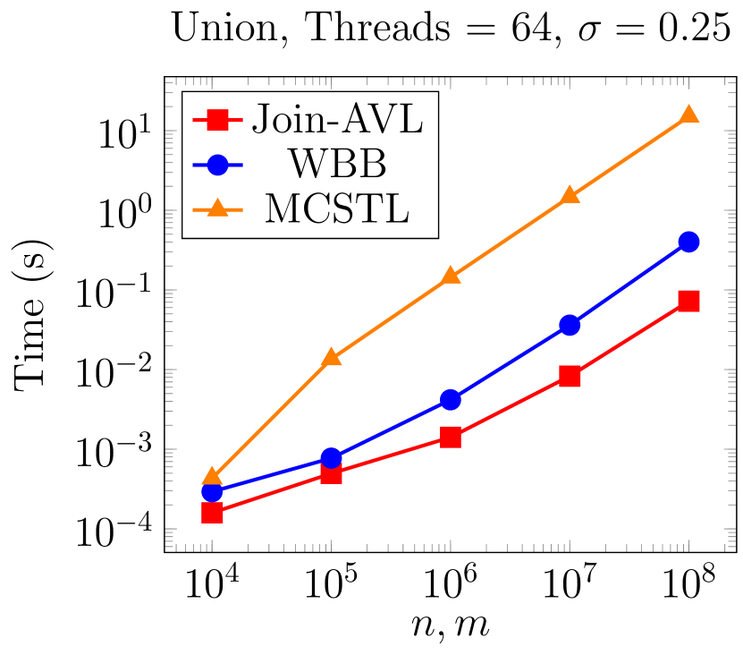
We test our algorithm by comparing it to other available implementations. This includes the sequential version of the set functions defined in the C++ Standard Template Library (STL) [20] and STL’s std::set (implemented by RB tree). The STL supports the set operations set_union, set_intersection, and set_difference on any container class. Using an std::vector these algorithms achieve a runtime of $O(m+n)$. Since the STL does not offer any parallel version of these functions we could only use it for sequential experiments. To see how well our algorithm performs in a parallel setting, we compare it to parallel WBB-trees [12] and the MCSTL library [13]. WBB-trees, as well as the MCSTL, offer support for bulk insertions and deletions. They process the bulk updates differently. The MCSTL first splits the main tree among $p$ processors, based on the bulk sequence, and then inserts the chunks dynamically into each subtree. The WBB-tree recursively inserts the bulk in parallel into the main tree. To deal with heavily skewed sequences they use partial tree reconstruction for fixing imbalances, which takes constant amortized time. The WBB-tree has a more cache aware layout, leading to a better cache utilization compared to both the MCSTL and our implementation. To make a comparison with these implementations we use their bulk insertions, which can also be viewed as an union of two sets. However notice that WBB-trees take the bulk in the form of a sorted sequence, which gives them an advantage due to the faster access to the one array than to a tree, and far better cache performance (8 keys per cache line as opposed to 1).

(a)

(b)

(c)

(d)

(e)

(f)

(g)

(h)

Figure 11: (a) Times for Union as a function of size ($n=10^{8}$) for different BBSTs; (b) speed up of Union for different BBSTs; (c) times for various operations on AVL trees as a function of size ($n=10^{8}$); (d) comparing STLs set_union with our Union; (e, f, g, h) comparing our Union to other parallel search trees; (e, h) input keys are uniformly distributed doubles in the range of [0, 1]; (f, g) inputs keys follow a normal distribution of doubles - the mean of the main tree is always $\mu_{1}=0$, while the mean of the bulk is $\mu_{2}=1$. Figure (f) uses a standard deviation of $\sigma=0.25$, while Figure (g) shows the performance across different standard deviations.

Comparing the balancing schemes and functions

To compare the four balancing schemes we choose Union as the representative operation. Other operations would lead to similar results since all operations except Join are generic across the trees. We compare the schemes across different thread counts and different sizes.

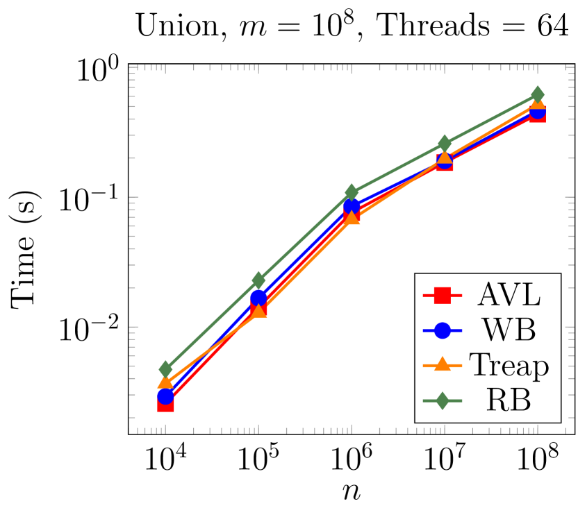
Figure 11 (a) shows the runtime of Union for various tree sizes and all four balancing schemes across 64 cores. The times are very similar among the balancing schemes—they differ by no more than 10%.

Figure 11 (b) shows the speedup curves for Union on varying core numbers with two inputs of size $10^{8}$. All balancing schemes achieve a speedup of about 45 on 64 cores, and about 30 on 32 cores. The less-than-linear speedup beyond 32 cores is not due to lack of parallelism, since when we ran the same experiments on significantly smaller input (and hence less parallelism) we get very similar curves (not shown). Instead it seems to be due to saturation of the memory bandwidth.

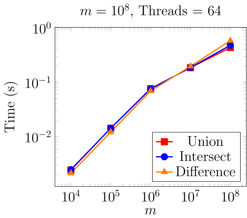
We use the AVL tree as the representative tree to compare different functions. Figure 11 (c) compares the Union, Intersect and Difference functions. The size of the larger tree is fixed ($10^{8}$), while the size of the smaller tree varies from $10^{4}$ to $10^{8}$. As the plot indicates, the three functions have very similar performance.

The experiments are a good indication of the performance of different balancing schemes and different functions, while controlling other factors. The conclusion is that all schemes perform almost equally on all the set functions. It is not surprising that all balancing schemes achieve similar performance because the dominant cost is in cache misses along the paths in the tree, and all schemes keep the trees reasonably balanced. The AVL tree is always slightly faster than the other trees and this is likely due to the fact that they maintain a slightly stricter balance than the other trees, and hence the paths that need to be traversed are slightly shorter. For different set functions the performance is also as expected given the similarity of the code.

Given the result that the four balancing schemes do not have a big difference in timing and speedup, nor do the three set functions, in the following experiments we use the AVL tree along with Union to make comparisons with other implementations.

Comparing to sequential implementations

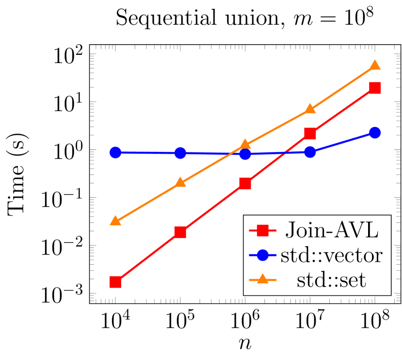
The STL supports set_union on any sorted container class, including sets based on red-black trees, and sorted vectors (arrays). The STL set_union merges the two sorted containers by moving from left to right on the two inputs, comparing the current values, and writing the lesser to the end of the output. For two inputs of size $n$ and $m$, $m\leq n$, it takes $O(m+n)$ time on std::vectors, and $O((n+m)\log(n+m))$ time on std::set (each insertion at the end of the output red-black tree takes $O(\log(n+m))$ time). In the case of ordered sets we can do better by inserting elements from the smaller set into the larger, leading a time of $O(m\log(n+m)$. This is also what we do in our experiments. For vectors we stick with the available set_union implementation.

Figure 11 (d) gives a comparison of times for Union. For equal lengths our implementation is about a factor of 3 faster than set variant (red-black trees), and about 8 times slower than the vector variant. This is not surprising since we are asymptotically faster than their red-black tree implementation, and their array-based implementation just reads and writes the values, one by one, from flat arrays, and therefore has much less overhead and much fewer cache misses. For taking the union of smaller and larger inputs, our Union is orders of magnitude faster than either STL version. This is because their theoretical work bound ($O(m+n)$ and $O(m\log(m+n)$) is worse than our $O(m\log(n/m+1))$, which is optimal in comparison model.

Comparing to parallel implementations on various input distributions

We compare our implementations to other parallel search trees, such as the WBB-trees, as described in [12], and parallel RB trees from the MCSTL [13]. We test the performance on different input distributions.

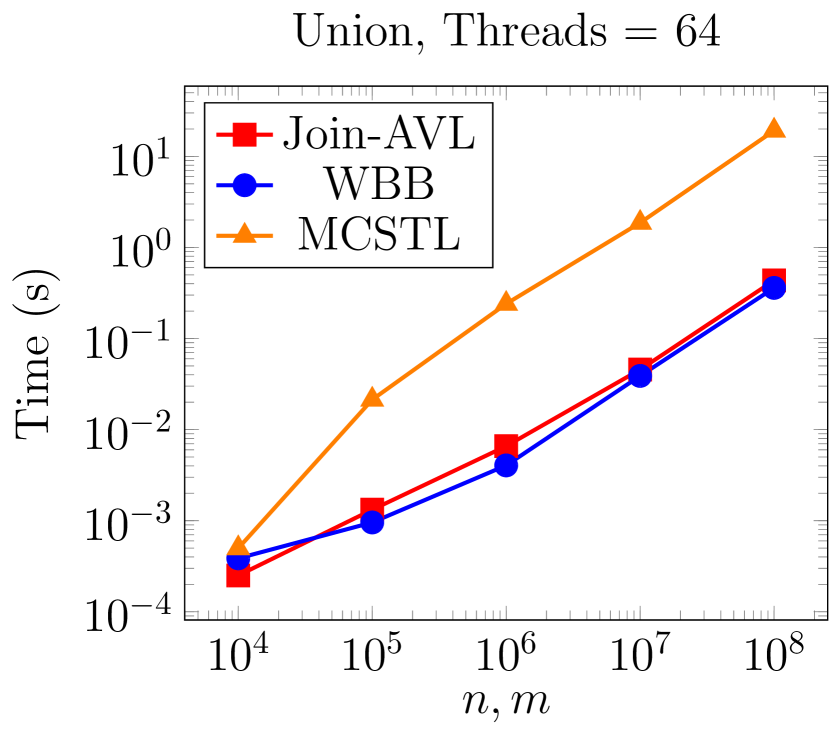
In Figure 11 (e) we show the result of Union on uniformly distributed doubles in the range of [0,1] across 64 cores. We set the input size to $n=m=10^{i}$, $i$ from $4$ to $8$. The three implementations have similar performance when $n=m=10^{4}$. As the input size increases, MCSTL shows much worse performance than the other two because of the lack of parallelism (Figure 11 (h) is a good indication), and the WBB-tree implementation is slightly better than ours. For the same reason that STL vectors outperform STL sets (implemented with RB trees) and our sequential implementation, the WBB-trees take the bulk as a sorted array, which has much less overhead to access and much better cache locality. Also their tree layout is more cache efficient and the overall height is lower since they store multiple keys per node.

Figure 11 (f) shows the result of a Gaussian distribution with doubles, also on all 64 cores with set sizes of $n=m=10^{i}$ for $i=4$ through $8$. The distributions of the two sets have means at $0$ and $1$ respectively, and both having a standard deviation of $0.25$, meaning that the data in the two sets have less overlap comparing to a uniform distribution (as in (e)). In this case our code achieves better performance than the other two implementations. For our algorithms less overlap in the data means more parts of the trees will be untouched, and therefore less nodes will be operated on. This in turn leads to less processing time.

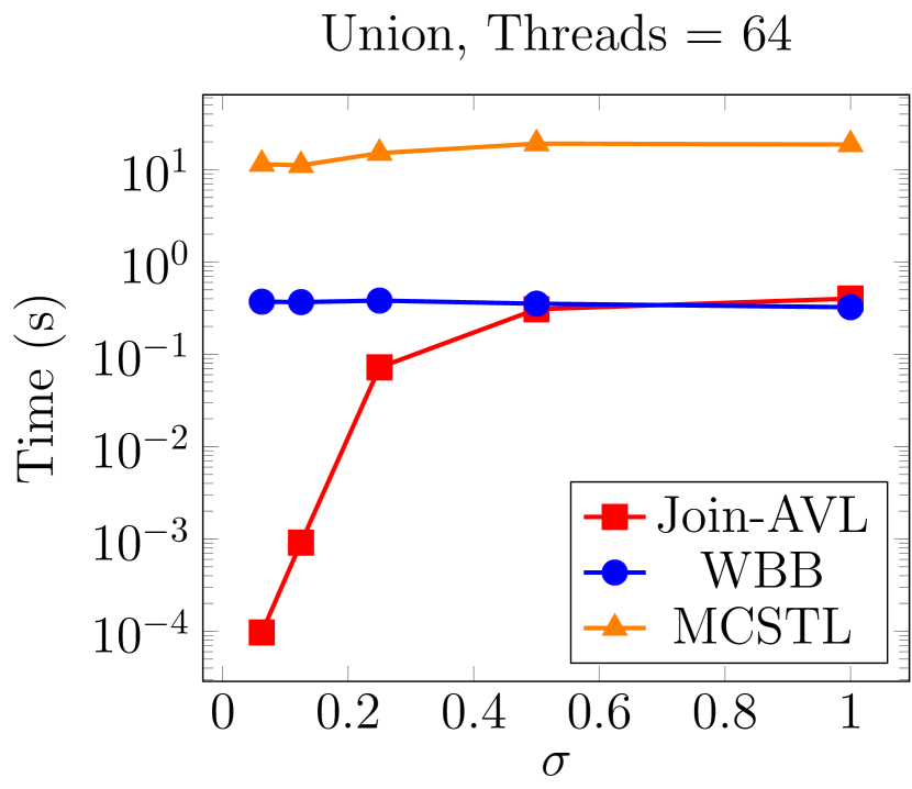
We also do an in-depth study on how the overlap of the data sets affects the performance of each algorithm. We generate two sets of size $n=m=10^{8}$, each from a Gaussian distribution. The distributions of the two sets have means at $0$ and $1$ respectively, and both have an equal standard deviation varying in $\{1,1/2,1/4,1/8,1/16\}$. The different standard deviations are to control the overlap of the two sets, and ideally less overlap should simplify the problem. Figure 11 (g) shows the result of the three parallel implementations on a Gaussian distribution with different standard deviations. From the figure we can see that MCSTL and WBB-tree are not affected by different standard deviations, while our join-based union takes advantage of less overlapping and achieves a much better performance when $\sigma$ is small. This is not surprising since when the two sets are less overlapped, e.g., totally disjoint, our Union will degenerate to a simple Join, which costs only $O(\log n)$ work. This behavior is consistent with the “adaptive” property (not always the worst-case) in [demaine2000adaptive]. This indicates that our algorithm is the only one among the three parallel implementations that can detect and take advantage of less overlapping in data, hence have a much better performance when the two operated sets are less overlapped.

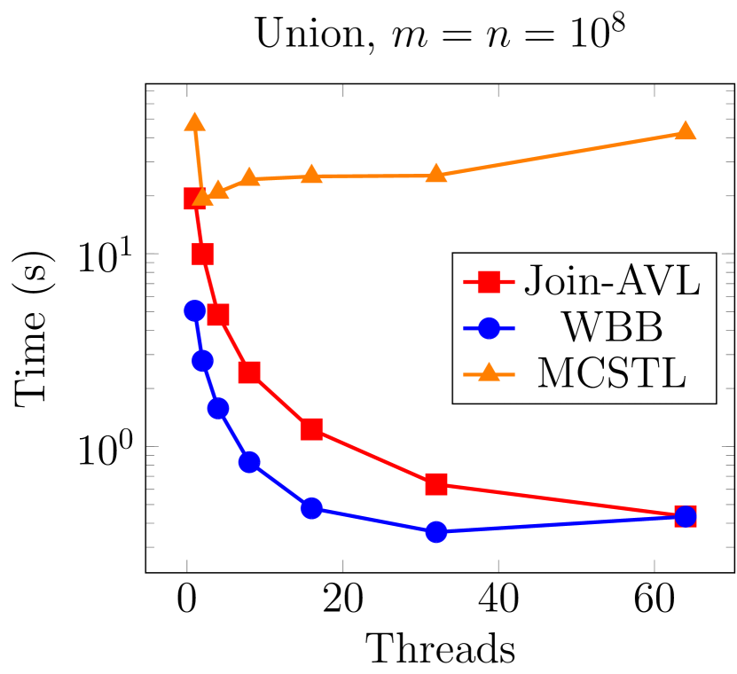
We also compare the parallelism of these implementations. In Figure 11 (h) we show their performance across 64 cores. The inputs are both of size $10^{8}$, and generated from an uniform distribution of doubles. It is easy to see that MCSTL does not achieve good parallelism beyond 16 cores, which explains why the MCSTL always performs the worst on 64 cores in all settings. As we mentioned earlier, the WBB-tree are slightly faster than our code, but when it comes to all 64 cores, both algorithms have similar performance. This indicates that our algorithm achieves better parallelism.

To conclude, in terms of parallel performance, our code and WBB-trees are always much better than the MCSTL because of MCSTL’s lack of parallelism. WBB-trees achieve a slightly better performance than ours on uniformly distributed data, but it does not improve when the two sets are less overlapped. Thus our code is much better than the other two implementations on less overlapped data, while still achieving a similar performance with the other algorithms when the two sets are more intermixed with each other.

7 Conclusions

In this paper, we study ordered sets implemented with balanced binary search trees. We show for the first time that a very simple “classroom-ready” set of algorithms due to Adams’ are indeed work optimal when used with four different balancing schemes–AVL, RB, WB trees and treaps—and also highly parallel. The only tree-specific algorithm that is necessary is the Join, and even the Joins are quite simple, as simple as Insert or Delete. It seems it is not sufficient to give a time bound to Join and base analysis on it. Indeed if this were the case it would have been done years ago. Instead our approach defines the notion of a rank (differently for different trees) and shows invariants on the rank. It is important that the cost of Join is proportional to the difference in ranks. It is also important that when joining two trees the resulting rank is only a constant bigger than the larger rank of the inputs. This insures that when joins are used in a recursive tree, as in Union, the ranks of the results in a pair of recursive calls does not differ much on the two sides. This then ensures that the set functions are efficient.

We also test the performance of our algorithm. Our experiments show that our sequential algorithm is about 3x faster for union on two maps of size $10^{8}$ compared to the STL red-black tree implementation. In parallel settings our code is much better than the two baseline algorithms (MCSTL and WBB-tree) on less overlapped data, while still achieves similar performances with WBB-tree when the two sets are more intermixed. Our code also achieves 45x speedup on 64 cores.

Appendix A Proofs for Some Lemmas

A.1 Proof for Lemma 8

Proof.

One observation in WB trees and treaps is that all nodes attached to a single layer root form a chain. This is true because if two children of one node $v$ are both in layer $i$, the weight of $v$ is more than $2^{i+1}$, meaning that $v$ should be layer $i+1$.

For a layer root $v$ in a WB tree on layer $k$, $w(v)$ is at most $2^{k+1}$. Considering the balance invariant that its child has weight at most $(1-\alpha)w(v)$, the weight of the $t$-th generation of its descendants is no more than $2^{k+1}(1-\alpha)^{t}$. This means that after $t^{*}=\log_{\frac{1}{1-\alpha}}2$ generations, the weight should decrease to less than $2^{k}$. Thus $d(v)\leq\log_{\frac{1}{1-\alpha}}2$, which is a constant.

For treaps consider a layer root $v$ on layer $k$ that has weight $N\in[2^{k},2^{k+1})$. The probability that $d(v)\geq 2$ is equal to the probability that one of its grandchildren has weight at least $2^{k}$. This probability $P$ is:

$$P =\frac{1}{2^{k}}\sum_{i=2^{k}+1}^{N}\frac{i-2^{k}}{i}$$ (7)

$$\leq\frac{1}{2^{k}}\sum_{i=2^{k}+1}^{2^{k+1}}\frac{i-2^{k}}{i}$$ (8)

$$\approx 1-\ln 2$$ (9)

We denote $1-\ln 2$ as $p_{c}$. Similarly, the probability that $d(v)\geq 4$ should be less than $p_{c}^{2}$, and the probability shrink geometrically as $d(v)$ increase. Thus the expected value of $d(v)$ is a constant.

Since treaps come from a random permutation, all $s(v)$ are i.i.d. ∎

A.2 Proof for Lemma 5

Proof.

We are trying to show that for $T_{r}=$Union$(T_{p},T_{d})$ on AVL, RB or WB trees, if $r(T_{p})>r(T_{d})$ then $r(T_{r})\leq r(T_{p})+r(T_{d})$.

For AVL and RB trees we use induction on $r(T_{p})+r(T_{d})$. When $r(T_{d})+r(T_{p})=1$ the conclusion is trivial. If $r=r(T_{p})>r(T_{d})$, $T_{p}$ will be split into two subtrees, with rank at most $r(T_{p})-1$ since we remove the root. $T_{d}$ will be split into two trees with height at most $r(T_{d})$ (Theorem 2). Using the inductive hypothesis, the two recursive calls will return two trees of height at most $r(T_{p})-1+r(T_{d})$. The result of the final Join is therefore at most $r(T_{p})+r(T_{d})$.

For WB trees, $|T|\leq|T_{p}|+|T_{d}|\leq 2|T_{p}|$. Thus $r(T)\leq r(T_{p})+1\leq r(T_{p})+r(T_{d})$. ∎

A.3 Proof for Lemma 3

Proof.

Figure 12: An illustration of two kinds of outcomes of rotation after joining two weight balanced trees. After we append the smaller tree to the larger one and rebalance from that point upwards, we reach the case in (0), where $u$ has been balanced, and the smaller tree has been part of it. Now we are balancing $v$, and two options are shown in (1) and (2). At least one of the two rotation will rebalance $v$.

Recall that in a weight balanced tree, for a certain node, neither of its children is $\beta$ times larger than the other one, where $\beta=\frac{1}{\alpha}-1$. When $\alpha\leq 1-\frac{1}{\sqrt{2}}$, we have $\beta\geq 1+\sqrt{2}$.

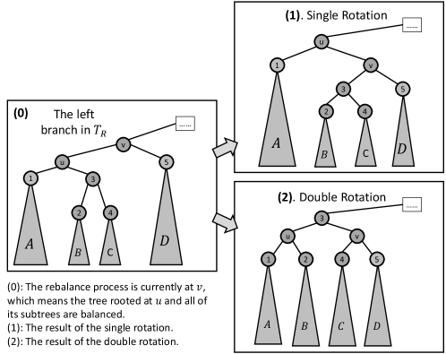
WLOG, we prove the case when $|T_{L}|<|T_{R}|$, where $T_{L}$ is inserted along the left branch of $T_{R}$. Then we rebalance the tree from the point of key $k$ and go upwards. As shown in Figure 12 (0), suppose the rebalance has been processed to $u$ (then we can use reduction). Thus the subtree rooted at $u$ is balanced, and $T_{L}$ is part of it. We name the four trees from left to right $A,B,C$ and $D$, and the number of nodes in them $a,b,c$ and $d$. From the balance condition we know that $A$ is balanced with $B+C$, and $B$ is balanced to $C$, i.e.:

$$\frac{1}{\beta}(b+c)\leq a\leq\beta(b+c)$$ (10)

$$\frac{1}{\beta}b\leq c\leq\beta c$$ (11)

We claim that at least one of the two operations will rebalanced the tree rooted at $v$ in Figure 12 (0):

1. Single rotation: right rotation at $u$ and $v$ (as shown in Figure 12 (1));

2. double rotation: Left rotation followed by a right rotation (as shown in Figure 12 (2)).

Also, notice that the inbalance is caused by the insertion of a subtree at the leftmost branch. Suppose the size of the smaller tree is $x$, and the size of the original left child of $v$ is $y$. Note that in the process of Join, $T_{L}$ is not concatenated with $v$. Instead, it goes down to deeper nodes. Also, note that the original subtree of size $y$ is weight balanced with $D$. This means we have:

$$x <\frac{1}{\beta}(d+y)$$

$$\frac{1}{\beta}d \leq y\leq\beta d$$

$$x+y =a+b+c$$

From the above three inequalities we get $x<\frac{1}{\beta}d+d$, thus:

$$a+b+c=x+y<(1+\beta+\frac{1}{\beta})d$$ (12)

Since a unbalance occurs, we have:

$$a+b+c>\beta d$$ (13)

We discuss the following 3 cases:

1. $\bm{B+C}$ is weight balanced with $\bm{D}$, i.e.,

   $${\frac{1}{\beta}}(b+c)\leq d\leq\beta(b+c)$$ (14)

   In this case, we apply a right rotate. The new tree rooted at $u$ is now balanced. $A$ is naturally balanced.

   Then we discuss in two cases:

   1. $\bm{\beta a\geq b+c+d}$.

      Notice that $b+c\geq{\frac{1}{\beta}}a$, meaning that $b+c+d>{\frac{1}{\beta}}a$. Then in this case, $A$ is balanced to $B+C+D$, $B+C$ is balanced to $D$. Thus just one right rotation will rebalance the tree rooted at $u$ (Figure 12 (1)).

   2. $\bm{\beta a<b+c+d}$.

      In this case, we claim that a double rotation as shown in Figure 12 (2) will rebalance the tree. Now we need to prove the balance of all the subtree pairs: $A$ with $B$, $C$ with $D$, and $A+B$ with $C+D$.

      First notice that when $\beta a<b+c+d$, from (13) we can get:

      $$\beta d<a+b+c<{\frac{1}{\beta}}(b+c+d)+b+c$$

      $$\Rightarrow (\beta-{\frac{1}{\beta}})d<({\frac{1}{\beta}}+1)(b+c)$$

      $$\Rightarrow (\beta-1)d<b+c$$ (15)

      Considering (14), we have $(\beta-1)d<b+c\leq\beta d$. Notice $b$ and $c$ satisfy (11), we have:

      $$b>\frac{1}{\beta+1}(b+c)>\frac{\beta-1}{\beta+1}d$$ (16)

      $$c>\frac{1}{\beta+1}(b+c)>\frac{\beta-1}{\beta+1}d$$ (17)

      Also note that when $\beta>1+\sqrt{2}\approx 2.414$, we have

      $$\frac{\beta+1}{\beta-1}<\beta$$ (18)

      We discuss the following three conditions of subtrees’ balance:

      1. Prove $\bm{A}$ is weight balanced to $\bm{B}$.

         1. Prove $\bm{b\leq\beta a}$.

            Since $\beta a\leq b+c$ (applying (10)) , we have $b\leq\beta a$.

         2. Prove $\bm{a\leq\beta b}$.

            In the case when $\beta a<b+c+d$ we have:

            $$a <\frac{1}{\beta}(b+c+d)~{}~{}~{}~{}{\rm{(applying{(\ref{btoc}),(\ref{btod})})}}$$

            $$<{\frac{1}{\beta}}(b+\beta b+\frac{\beta+1}{\beta-1}b)$$

            $$=\frac{\beta+1}{\beta-1}b$$

            $$<\beta b$$

      2. Prove $\bm{C}$ is weight balanced to $\bm{D}$.

         1. Prove $\bm{c\leq\beta d}$.

            Since $b+c\leq\beta d$ (applying (14)), we have $c\leq\beta d$.

         2. Prove $\bm{d\leq\beta c}$.

            From (17), we have

            $$d<\frac{\beta+1}{\beta-1}c<\beta c$$

      3. Prove $\bm{A+B}$ is weight balanced to $\bm{C+D}$.

         1. Prove $\bm{a+b\leq\beta(c+d)}$.

            From (15), (11) and (18) we have:

            $$d<\frac{1}{\beta-1}(b+c)\leq\frac{1}{\beta-1}(\beta c+c)$$

            $$=\frac{\beta+1}{\beta-1}c<\beta c$$

            $$\Rightarrow {\frac{1}{\beta}}d<c$$

            $$\Rightarrow (1+{\frac{1}{\beta}})d<(1+\beta)c$$

            $$\Rightarrow (1+{\frac{1}{\beta}}+\beta)d<\beta(c+d)+c~{}~{}{({\rm{applying~{}(\ref{a+b+csmallerd})}})}$$

            $$\Rightarrow a+b+c<(1+{\frac{1}{\beta}}+\beta)d<\beta(c+d)+c$$

            $$\Rightarrow a+b<\beta(c+d)$$

         2. Prove $\bm{c+d\leq\beta(a+b)}$.

            When $\beta>2$, we have $\frac{\beta}{\beta-1}<\beta$. Thus applying (15) and (10) we have:

            $$d<\frac{1}{\beta-1}(b+c)\leq\frac{\beta}{\beta-1}a<\beta a$$

            Also we have $c\leq\beta b$ (applying (11)). Thus $c+d<\beta(a+b)$.

2. $\bm{B+C}$ is too light that cannot be balanced with $\bm{D}$, i.e.,

   $$\beta(b+c)<d$$ (19)

   In this case, we have $a<\beta(b+c)<d$ (applying (10) and (19)), which means that $a+b+c<d+{\frac{1}{\beta}}d<\beta d$ when $\beta>\frac{1+\sqrt{5}}{2}\approx 1.618$. This contradicts with the condition that $A+B+C$ is too heavy to $D$ ($a+b+c>\beta d$). Thus this case is impossible.

3. $\bm{B+C}$ is too heavy that cannot be balanced with $\bm{D}$, i.e.,

   $$b+c>\beta d$$ (20)

   $$\Rightarrow a>{\frac{1}{\beta}}(b+c)>d$$ (21)

   In this case, we apply the double rotation.

   We need to prove the following balance conditions:

   1. Prove $\bm{A}$ is weight balanced to $\bm{B}$.

      1. Prove $\bm{b<\beta a}$.

         Since $\beta a>b+c$ (applying (10)) , we have $b<\beta a$.

      2. Prove $\bm{a<\beta b}$.

         Suppose $c=kb$, where ${\frac{1}{\beta}}<k<\beta$. Since $b+c>\beta d$, we have:

         $$d<\frac{1+k}{\beta}b$$ (22)

         From the above inequalities, we have:

         $$a+b+c =a+b+kb~{}~{}~{}~{}~{}~{}~{}~{}({\rm{applying(\ref{a+b+csmallerd}}}))$$

         $$<(1+\beta+{\frac{1}{\beta}})d~{}~{}~{}({\rm{applying(\ref{dtob}}}))$$

         $$<(1+\beta+{\frac{1}{\beta}})\times\frac{1+k}{\beta}b$$

         $$\Rightarrow a <\mathopen{}\mathclose{{}\left(\frac{1+\beta+{\frac{1}{\beta}}}{\beta}-1}\right)(1+k)b$$

         $$=\frac{\beta+1}{\beta^{2}}(1+k)b$$

         $$<\frac{(\beta+1)^{2}}{\beta^{2}}b$$

         When $\beta>\frac{7}{9}\times(\frac{\sqrt{837}+47}{54})^{-1/3}+(\frac{\sqrt{837}+47}{54})^{1/3}+\frac{1}{3}\approx 2.1479$, we have $\frac{(\beta+1)^{2}}{\beta}<\beta$. Hence $a<\beta b$.

   2. Prove $\bm{C}$ is weight balanced to $\bm{D}$.

      1. Prove $\bm{d\leq\beta c}$.

         When $\beta>\frac{1+\sqrt{5}}{2}\approx 1.618$, we have $\beta>1+{\frac{1}{\beta}}$. Assume to the contrary $c<{\frac{1}{\beta}}d$, we have $b<\beta c<d$. Thus:

         $$b+c<(1+{\frac{1}{\beta}})d<\beta d$$

         , which contradicts with (20) that $B+C$ is too heavy to be balanced with $D$.

      2. Prove $\bm{c<\beta d}$.

         Plug (21) in (12) and get $b+c<(\beta+{\frac{1}{\beta}})d$. Recall that $\beta>1$, we have:

         $${\frac{1}{\beta}}c+c<b+c<(\beta+{\frac{1}{\beta}})d$$

         $$\Rightarrow c<\frac{\beta^{2}+1}{\beta+1}d<\beta d$$

   3. Prove $\bm{A+B}$ is weight balanced with $\bm{C+D}$.

      1. Prove $\bm{c+d\leq\beta(a+b)}$.

         From (11) we have $c<\beta b$, also $d<a<\beta a$ (applying (21)), thus $c+d<\beta(a+b)$.

      2. Prove $\bm{a+b\leq\beta(c+d)}$.

         Recall when $\beta>\frac{1+\sqrt{5}}{2}\approx 1.618$, we have $\beta>1+{\frac{1}{\beta}}$. Applying (20) and (11) we have:

         $$d\leq{\frac{1}{\beta}}(b+c)\leq c+{\frac{1}{\beta}}c<\beta c$$

         $$\Rightarrow {\frac{1}{\beta}}d<c$$

         $$\Rightarrow (1+{\frac{1}{\beta}})d<(1+\beta)c$$

         $$\Rightarrow (1+{\frac{1}{\beta}}+\beta)d<\beta(c+d)+c~{}~{}{({\rm{applying~{}(\ref{a+b+csmallerd})}})}$$

         $$\Rightarrow a+b+c<(1+{\frac{1}{\beta}}+\beta)d<\beta(c+d)+c$$

         $$\Rightarrow a+b<\beta(c+d)$$

Taking all the three conclusions into consideration, after either a single rotation or a double rotation, the new subtree will be rebalanced.

Then by induction we can prove Lemma 3. ∎

References

- [1] S. Adams. Implementing sets effciently in a functional language. Technical Report CSTR 92-10, University of Southampton, 1992.
- [2] S. Adams. Efficient sets—a balancing act. Journal of functional programming, 3(04):553–561, 1993.
- [3] G. Adelson-Velsky and E. M. Landis. An algorithm for the organization of information. Proc. of the USSR Academy of Sciences, 145:263–266, 1962. In Russian, English translation by Myron J. Ricci in Soviet Doklady, 3:1259-1263, 1962.
- [4] Y. Akhremtsev and P. Sanders. Fast parallel operations on search trees(unpublished), 2016.
- [5] R. Bayer. Symmetric binary b-trees: Data structure and maintenance algorithms. Acta Informatica, 1:290–306, 1972.
- [6] G. E. Blelloch and M. Reid-Miller. Fast set operations using treaps. In Proc. ACM Symposium on Parallel Algorithms and Architectures (SPAA), pages 16–26, 1998.
- [7] N. Blum and K. Mehlhorn. On the average number of rebalancing operations in weight-balanced trees. Theoretical Computer Science, 11(3):303–320, 1980.
- [8] R. D. Blumofe and C. E. Leiserson. Space-efficient scheduling of multithreaded computations. SIAM J. on Computing, 27(1):202–229, 1998.
- [9] R. P. Brent. The parallel evaluation of general arithmetic expressions. Journal of the ACM, 21(2):201–206, Apr. 1974.
- [10] N. G. Bronson, J. Casper, H. Chafi, and K. Olukotun. A practical concurrent binary search tree. In Proc. ACM SIGPLAN Symp. on Principles and Practice of Parallel Programming (PPoPP), pages 257–268, 2010.
- [11] M. R. Brown and R. E. Tarjan. A fast merging algorithm. Journal of the ACM (JACM), 26(2):211–226, 1979.
- [12] S. Erb, M. Kobitzsch, and P. Sanders. Parallel bi-objective shortest paths using weight-balanced b-trees with bulk updates. In Experimental Algorithms, pages 111–122. Springer, 2014.
- [13] L. Frias and J. Singler. Parallelization of bulk operations for STL dictionaries. In Euro-Par 2007 Workshops: Parallel Processing, HPPC 2007, UNICORE Summit 2007, and VHPC 2007, pages 49–58, 2007.
- [14] Y. Hirai and K. Yamamoto. Balancing weight-balanced trees. Journal of Functional Programming, 21(03):287–307, 2011.
- [15] F. K. Hwang and S. Lin. A simple algorithm for merging two disjoint linearly ordered sets. SIAM J. on Computing, 1(1):31–39, 1972.
- [16] J. Katajainen. Efficient parallel algorithms for manipulating sorted sets. In Proceedings of the 17th Annual Computer Science Conference. University of Canterbury, 1994.
- [17] H. T. Kung and P. L. Lehman. Concurrent manipulation of binary search trees. ACM Trans. Database Syst., 5(3):354–382, 1980.
- [18] K. S. Larsen. AVL trees with relaxed balance. J. Comput. Syst. Sci., 61(3):508–522, 2000.
- [19] S. Marlow et al. Haskell 2010 language report. Available online http://www. haskell. org/(May 2011), 2010.
- [20] D. R. Musser, G. J. Derge, and A. Saini. STL tutorial and reference guide: C++ programming with the standard template library. Addison-Wesley Professional, 2009.
- [21] A. Natarajan and N. Mittal. Fast concurrent lock-free binary search trees. In Proc. ACM SIGPLAN Symp. on Principles and Practice of Parallel Programming (PPoPP), pages 317–328, 2014.
- [22] J. Nievergelt and E. M. Reingold. Binary search trees of bounded balance. SIAM J. Comput., 2(1):33–43, 1973.
- [23] H. Park and K. Park. Parallel algorithms for red–black trees. Theoretical Computer Science, 262(1):415–435, 2001.
- [24] W. J. Paul, U. Vishkin, and H. Wagener. Parallel dictionaries in 2-3 trees. In Proc. Intl. Colloq. on Automata, Languages and Programming (ICALP), pages 597–609, 1983.
- [25] R. Seidel and C. R. Aragon. Randomized search trees. Algorithmica, 16:464–497, 1996.
- [26] D. D. Sleator and R. E. Tarjan. Self-adjusting binary search trees. Journal of the ACM (JACM), 32(3):652–686, 1985.
- [27] M. Straka. Adams’ trees revisited. In Trends in Functional Programming, pages 130–145. Springer, 2012.
- [28] R. E. Tarjan. Data Structures and Network Algorithms. Society for Industrial and Applied Mathematics, Philadelphia, PA, USA, 1983.