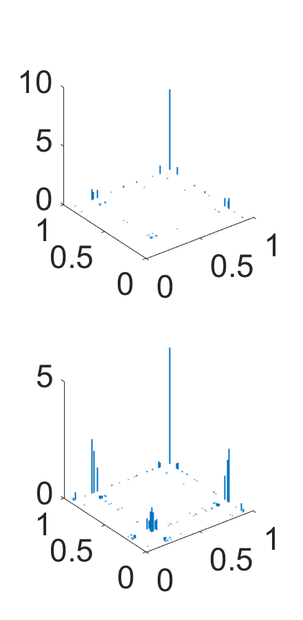
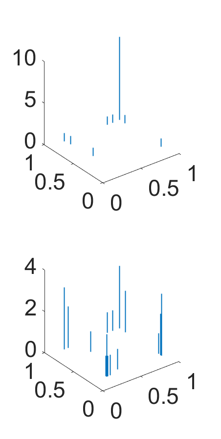
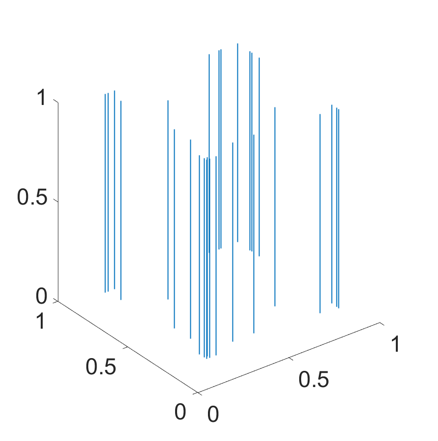
, and

Exchangeable Random Measures for Sparse and Modular Graphs with Overlapping Communities

Adrien Todeschinilabel=e2]Adrien.Todeschini@inria.fr [    Xenia Miscouridoulabel=e3]xenia.miscouridou@spc.ox.ac.uk [    François Caronlabel=e1]caron@stats.ox.ac.uk [ INRIA and University of Oxford INRIA & Institut de Mathématiques de Bordeaux, France
Department of Statistics, University of Oxford, UK
Abstract

We propose a novel statistical model for sparse networks with overlapping community structure. The model is based on representing the graph as an exchangeable point process, and naturally generalizes existing probabilistic models with overlapping block-structure to the sparse regime. Our construction builds on vectors of completely random measures, and has interpretable parameters, each node being assigned a vector representing its level of affiliation to some latent communities. We develop methods for simulating this class of random graphs, as well as to perform posterior inference. We show that the proposed approach can recover interpretable structure from two real-world networks and can handle graphs with thousands of nodes and tens of thousands of edges.

keywords:
Networks, Random Graphs, Multiview Networks, Multigraphs, Completely Random Measures, Lévy measure, Multivariate Subordinator, Sparsity, Non-Negative Factorization, Exchangeability, Point Processes

1 Introduction

There has been a growing interest in the analysis, understanding and modeling of network data over the recent years. A network is composed of a set of nodes, or vertices, with connections between them. Network data arise in a wide range of fields, and include social networks, collaboration networks, communication networks, biological networks, food webs and are a useful way of representing interactions between sets of objects. Of particular importance is the elaboration of random graph models, which can capture the salient properties of real-world graphs. Following the seminal work of Erdös and Rényi (1959), various network models have been proposed; see the overviews of Newman (2003b, 2009), Kolaczyk (2009), Bollobás (2001), Goldenberg et al. (2010), Fienberg (2012) or Jacobs and Clauset (2014). In particular, a large body of the literature has concentrated on models that can capture some modular or community structure within the network. The first statistical network model in this line of research is the popular stochastic block-model (Holland et al., 1983; Snijders and Nowicki, 1997; Nowicki and Snijders, 2001). The stochastic block-model assumes that each node belongs to one of p𝑝p latent communities, and the probability of connection between two nodes is given by a p×p𝑝𝑝p\times p connectivity matrix. This model has been extended in various directions, by introducing degree-correction parameters (Karrer and Newman, 2011), by allowing the number of communities to grow with the size of the network (Kemp et al., 2006), or by considering overlapping communities (Airoldi et al., 2008; Miller et al., 2009; Latouche et al., 2011; Palla et al., 2012; Yang and Leskovec, 2013). Stochastic block-models and their extensions have shown to offer a very flexible modeling framework, with interpretable parameters, and have been successfully used for the analysis of numerous real-world networks. However, as outlined by Orbanz and Roy (2015), when one makes the usual assumption that the ordering of the nodes is irrelevant in the definition of the statistical network model, the Bayesian probabilistic versions of those models lead to dense networks111We refer to graphs whose number of edges scales quadratically with the number of nodes as dense, and sparse if it scales sub-quadratically.: that means that the number of edges grows quadratically with the number of nodes. This property is rather undesirable, as many real-world networks are believed to be sparse.

Recently, Caron and Fox (2017) proposed an alternative framework for statistical network modeling. The framework is based on representing the graph as an exchangeable random measure on the plane. More precisely, the nodes are embedded at some location θi+subscript𝜃𝑖subscript\theta_{i}\in\mathbb{R}_{+} and, for simple graphs, a connection exists between two nodes i𝑖i and j𝑗j if there is a point at locations (θi,θj)subscript𝜃𝑖subscript𝜃𝑗(\theta_{i},\theta_{j}) and (θj,θi)subscript𝜃𝑗subscript𝜃𝑖(\theta_{j},\theta_{i}). An undirected simple graph is therefore represented by a symmetric point process Z𝑍Z on the plane

Z=i,jzijδ(θi,θj)𝑍subscript𝑖𝑗subscript𝑧𝑖𝑗subscript𝛿subscript𝜃𝑖subscript𝜃𝑗Z=\sum_{i,j}z_{ij}\delta_{(\theta_{i},\theta_{j})} (1)

where zij=zji=1subscript𝑧𝑖𝑗subscript𝑧𝑗𝑖1z_{ij}=z_{ji}=1 if i𝑖i and j𝑗j are connected, 0 otherwise; see Figure 1 for an illustration. Caron and Fox (2017) noted that jointly exchangeable random measures, a notion to be defined in Eq. (23), admit a representation theorem due to Kallenberg (1990), providing a general construction for exchangeable random measures hence random graphs represented by such objects. This connection is further explored by Veitch and Roy (2015) and Borgs et al. (2016), who provide a detailed description and extensive theoretical analysis of the associated class of random graphs, which they name Kallenberg exchangeable graphs or graphon processes. Within this class of models, Caron and Fox (2017) consider in particular the following simple generative model, where two nodes ij𝑖𝑗i\neq j connect with probability

Pr(zij=1|(w)=1,2,)=1e2wiwjPrsubscript𝑧𝑖𝑗conditional1subscriptsubscript𝑤121superscript𝑒2subscript𝑤𝑖subscript𝑤𝑗\Pr(z_{ij}=1|(w_{\ell})_{\ell=1,2,\ldots})=1-e^{-2w_{i}w_{j}} (2)

where the (wi,θi)i=1,2,subscriptsubscript𝑤𝑖subscript𝜃𝑖𝑖12(w_{i},\theta_{i})_{i=1,2,\ldots} are the points of a Poisson point process on +2superscriptsubscript2\mathbb{R}_{+}^{2}. The parameters wi>0subscript𝑤𝑖0w_{i}>0 can be interpreted as sociability parameters. Depending on the properties of the mean measure of the Poisson process, the authors show that it is possible to generate both dense and sparse graphs, with potentially heavy-tailed degree distributions, within this framework. The construction (2) is however rather limited in terms of capturing structure in the network. Herlau et al. (2015) proposed an extension of (2), which can accommodate a community structure. More precisely, introducing latent community membership variables ci{1,,p}subscript𝑐𝑖1𝑝c_{i}\in\{1,\ldots,p\}, two nodes ij𝑖𝑗i\neq j connect with probability

Pr(zij=1|(w,c)=1,2,,(ηk)1k,p)=1e2ηcicjwiwjPrsubscript𝑧𝑖𝑗conditional1subscriptsubscript𝑤subscript𝑐12subscriptsubscript𝜂𝑘formulae-sequence1𝑘𝑝1superscript𝑒2subscript𝜂subscript𝑐𝑖subscript𝑐𝑗subscript𝑤𝑖subscript𝑤𝑗\Pr(z_{ij}=1|(w_{\ell},c_{\ell})_{\ell=1,2,\ldots},(\eta_{k\ell})_{1\leq k,\ell\leq p})=1-e^{-2\eta_{c_{i}c_{j}}w_{i}w_{j}} (3)

where the (wi,ci,θi)i=1,2,subscriptsubscript𝑤𝑖subscript𝑐𝑖subscript𝜃𝑖𝑖12(w_{i},{c_{i}},\theta_{i})_{i=1,2,\ldots} are the points of a (marked) Poisson point process on +×{1,,p}×+subscript1𝑝subscript\mathbb{R}_{+}\times\{1,\ldots,p\}\times\mathbb{R}_{+} and ηksubscript𝜂𝑘\eta_{k\ell} are positive random variables parameterizing the strength of interaction between nodes in community k𝑘k and nodes in community \ell. The model is similar in spirit to the degree-corrected stochastic block-model (Karrer and Newman, 2011), but within the point process framework (1), and can thus accommodate both sparse and dense networks with community structure. The model of Herlau et al. (2015) however shares the limitations of the (degree-corrected) stochastic block-model, in the sense that it cannot model overlapping community structures, each node being assigned to a single community; see Latouche et al. (2011) and Yang and Leskovec (2013) for more discussion along these lines. Other extensions with block structure or mixed membership block structure are also suggested by Borgs et al. (2016).

In this paper, we consider that each node i𝑖i is assigned a set of latent non-negative parameters wiksubscript𝑤𝑖𝑘w_{ik}, k=1,,p𝑘1𝑝k=1,\ldots,p, and that the probability that two nodes ij𝑖𝑗i\neq j connect is given by

Pr(zij=1|(w1,,wp)=1,2,)=1e2k=1pwikwjk.Prsubscript𝑧𝑖𝑗conditional1subscriptsubscript𝑤1subscript𝑤𝑝121superscript𝑒2superscriptsubscript𝑘1𝑝subscript𝑤𝑖𝑘subscript𝑤𝑗𝑘\Pr(z_{ij}=1|(w_{\ell 1},\ldots,w_{\ell p})_{\ell=1,2,\ldots})=1-e^{-2\sum_{k=1}^{p}w_{ik}w_{jk}}. (4)

These non-negative weights can be interpreted as measuring the level of affiliation of node i𝑖i to the latent communities k=1,,p𝑘1𝑝k=1,\ldots,p. For example, in a friendship network, these communities can correspond to colleagues, family, or sport partners, and the weights measure the level of affiliation of an individual to each community. Note that as individuals can have high weights in different communities, the model can capture overlapping communities. The link probability (4) builds on a non-negative factorization; it has been used by other authors for network modeling (Yang and Leskovec, 2013; Zhou, 2015) and is also closely related to the model for multigraphs of Ball et al. (2011). The main contribution of this paper is to use the link probability (4) within the point process framework of Caron and Fox (2017). To this aim, we consider that the node locations and weights (wi1,,wip,θi)i=1,2,subscriptsubscript𝑤𝑖1subscript𝑤𝑖𝑝subscript𝜃𝑖𝑖12(w_{i1},\ldots,w_{ip},\theta_{i})_{i=1,2,\ldots} are drawn from a Poisson point process on +p+1superscriptsubscript𝑝1\mathbb{R}_{+}^{p+1} with a given mean measure ν𝜈\nu. The construction of such multivariate point process relies on vectors of completely random measures (or equivalently multivariate subordinators). In particular, we build on the flexible though tractable construction recently introduced by Griffin and Leisen (2017).

The proposed model generalizes that of Caron and Fox (2017) by allowing the model to capture more structure in the network, while retaining its main features, and is shown to have the following properties:

  • Interpretability: each node is assigned a set of positive parameters, which can be interpreted as measuring the levels of affiliation of a node to latent communities; once those parameters are learned, they can be used to undercover the latent structure in the network.

  • Sparsity: we can generate graphs whose number of edges grows subquadratically with the number of nodes.

  • Exchangeability: in the sense of Kallenberg (1990).

Additionally, we develop a Markov chain Monte Carlo (MCMC) algorithm for posterior inference with this model, and show experiments on two real-world networks with a thousand of nodes and tens of thousands of edges.

The article is organized as follows. The class of random graph models is introduced in Section 2. Properties of the class of graphs and simulation are described in Section 3. We derive a scalable MCMC algorithm for posterior inference in Section 4. In Section 5 we provide illustrations of the proposed method on simulated data and on two networks: a network of citations between political blogs and a network of connections between US airports. We show that the approach is able to discover interpretable structure in the data and performs well compared to alternatives.

0zijsubscript𝑧𝑖𝑗\color[rgb]{0,0,0.3}\definecolor[named]{pgfstrokecolor}{rgb}{0,0,0.3}z_{ij}θisubscript𝜃𝑖\color[rgb]{0,0,0}\definecolor[named]{pgfstrokecolor}{rgb}{0,0,0}\pgfsys@color@gray@stroke{0}\pgfsys@color@gray@fill{0}\theta_{i}θjsubscript𝜃𝑗\color[rgb]{0,0,0}\definecolor[named]{pgfstrokecolor}{rgb}{0,0,0}\pgfsys@color@gray@stroke{0}\pgfsys@color@gray@fill{0}\theta_{j}wi1subscript𝑤𝑖1\color[rgb]{0,0.7,0}\definecolor[named]{pgfstrokecolor}{rgb}{0,0.7,0}w_{i1}wi2subscript𝑤𝑖2\color[rgb]{1,0,0}\definecolor[named]{pgfstrokecolor}{rgb}{1,0,0}w_{i2}wi3subscript𝑤𝑖3\color[rgb]{0,0,1}\definecolor[named]{pgfstrokecolor}{rgb}{0,0,1}w_{i3}wj1subscript𝑤𝑗1\color[rgb]{0,0.7,0}\definecolor[named]{pgfstrokecolor}{rgb}{0,0.7,0}w_{j1}wj2subscript𝑤𝑗2\color[rgb]{1,0,0}\definecolor[named]{pgfstrokecolor}{rgb}{1,0,0}w_{j2}wj3subscript𝑤𝑗3\color[rgb]{0,0,1}\definecolor[named]{pgfstrokecolor}{rgb}{0,0,1}w_{j3}
Figure 1: Representation of a undirected graph via a point process Z𝑍Z. Each node i𝑖i is embedded in +subscript\mathbb{R}_{+} at some location θisubscript𝜃𝑖\theta_{i} and is associated with a set of positive attributes (wi1,,wip)subscript𝑤𝑖1subscript𝑤𝑖𝑝(w_{i1},\ldots,w_{ip}). An edge between nodes θisubscript𝜃𝑖\theta_{i} and θjsubscript𝜃𝑗\theta_{j} is represented by a point at locations (θi,θj)subscript𝜃𝑖subscript𝜃𝑗(\theta_{i},\theta_{j}) and (θj,θi)subscript𝜃𝑗subscript𝜃𝑖(\theta_{j},\theta_{i}) in +2superscriptsubscript2\mathbb{R}_{+}^{2}.

2 Sparse graph models with overlapping communities

In this section, we present the statistical model for simple graphs. The construction builds on vectors of completely random measures (CRM, Kingman, 1967). We only provide here the necessary material for the definition of the network model; please refer to Appendix A for additional background on vectors of CRMs. The model described in this section can also be extended to bipartite graphs; see Appendix E.

2.1 General construction using vectors of CRMs

We consider that each node i𝑖i is embedded at some location θi+subscript𝜃𝑖subscript\theta_{i}\in\mathbb{R}_{+}, and has some set of positive weights (wi1,,wip)+psubscript𝑤𝑖1subscript𝑤𝑖𝑝superscriptsubscript𝑝(w_{i1},\ldots,w_{ip})\in\mathbb{R}_{+}^{p}. The points (wi1,,wip,θi)i=1,,subscriptsubscript𝑤𝑖1subscript𝑤𝑖𝑝subscript𝜃𝑖𝑖1(w_{i1},\ldots,w_{ip},\theta_{i})_{i=1,\ldots,\infty} are assumed to be drawn from a Poisson process with mean measure

ν(dw1,,dwp,dθ)=ρ(dw1,,dwp)λ(dθ)𝜈𝑑subscript𝑤1𝑑subscript𝑤𝑝𝑑𝜃𝜌𝑑subscript𝑤1𝑑subscript𝑤𝑝𝜆𝑑𝜃\nu(dw_{1},\ldots,dw_{p},d\theta)=\rho(dw_{1},\ldots,dw_{p})\lambda(d\theta) (5)

where λ𝜆\lambda is the Lebesgue measure and ρ𝜌\rho is a σ𝜎\sigma-finite measure on +psubscriptsuperscript𝑝\mathbb{R}^{p}_{+}, concentrated on +p\{𝟎}\subscriptsuperscript𝑝0\mathbb{R}^{p}_{+}\backslash\{\mathbf{0}\}, which satisfies

+pmin(1,k=1pwk)ρ(dw1,,dwp)<.subscriptsuperscriptsubscript𝑝1superscriptsubscript𝑘1𝑝subscript𝑤𝑘𝜌𝑑subscript𝑤1𝑑subscript𝑤𝑝\int_{\mathbb{R}_{+}^{p}}\min\left(1,\sum_{k=1}^{p}w_{k}\right)\rho(dw_{1},\ldots,dw_{p})<\infty. (6)

Under this condition (Skorohod, 1991; Barndorff-Nielsen et al., 2001), we can describe the set of weights and locations using a vector of completely random measures (W1,,Wp)subscript𝑊1subscript𝑊𝑝(W_{1},\ldots,W_{p}) on +subscript\mathbb{R}_{+}:

Wk=i=1wikδθi, for k=1,,p.formulae-sequencesubscript𝑊𝑘superscriptsubscript𝑖1subscript𝑤𝑖𝑘subscript𝛿subscript𝜃𝑖 for 𝑘1𝑝W_{k}=\sum_{i=1}^{\infty}w_{ik}\delta_{\theta_{i}},\text{ for }k=1,\ldots,p. (7)

We simply write

(W1,,Wp)CRM(ρ,λ).similar-tosubscript𝑊1subscript𝑊𝑝CRM𝜌𝜆(W_{1},\ldots,W_{p})\sim\text{CRM}(\rho,\lambda). (8)
Refer to caption
Refer to caption
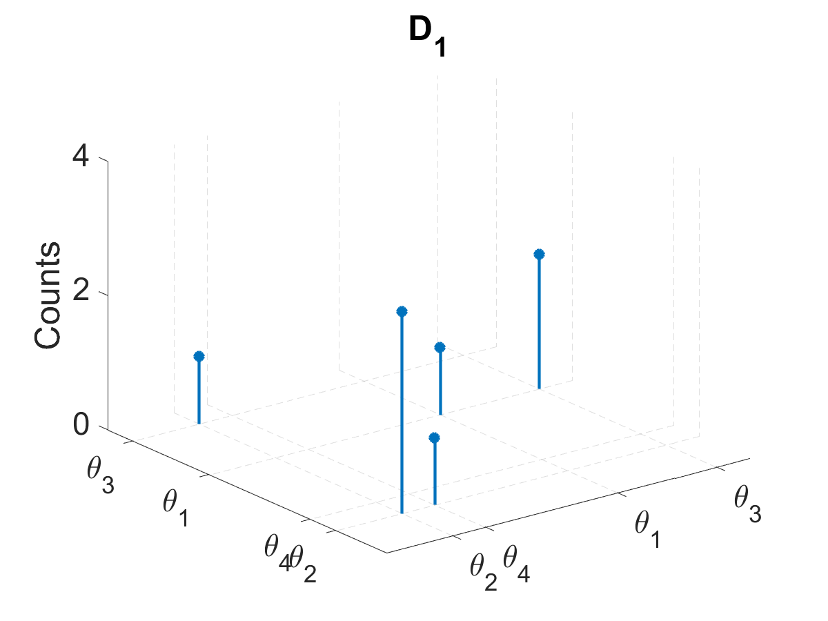
θ1subscript𝜃1\theta_{1}θ2subscript𝜃2\theta_{2}θ3subscript𝜃3\theta_{3}θ4subscript𝜃4\theta_{4}333111111111222
θ1subscript𝜃1\theta_{1}θ2subscript𝜃2\theta_{2}θ3subscript𝜃3\theta_{3}444222111333
θ1subscript𝜃1\theta_{1}θ2subscript𝜃2\theta_{2}θ3subscript𝜃3\theta_{3}θ4subscript𝜃4\theta_{4}
(a)   (b)   (c)
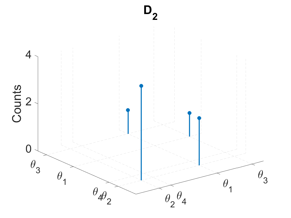
Figure 2: An example of (a) the restriction on [0,1]2superscript012[0,1]^{2} of the two atomic measures D1subscript𝐷1D_{1} and D2subscript𝐷2D_{2}, (b) the corresponding multiview directed multigraphs (top: view 1; bottom: view 2) and (c) corresponding undirected graph.
Refer to caption
(a) Wk×Wksubscript𝑊𝑘subscript𝑊𝑘W_{k}\times W_{k}
Refer to caption
(b) Integer point processes Dksubscript𝐷𝑘D_{k}
Refer to caption
(c) Point process Z𝑍Z
Figure 3: An example, for p=2𝑝2p=2, of (a) the product measures Wk×Wksubscript𝑊𝑘subscript𝑊𝑘W_{k}\times W_{k}, (b) a draw of the directed multigraph measures DkWkPoisson(Wk×Wk)similar-toconditionalsubscript𝐷𝑘subscript𝑊𝑘Poissonsubscript𝑊𝑘subscript𝑊𝑘D_{k}\mid W_{k}\sim{\operatorname{Poisson}}(W_{k}\times W_{k}) and (c) corresponding undirected measure Z=i=1j=1min(1,k=1pnijk+njik)δ(θi,θj)𝑍superscriptsubscript𝑖1superscriptsubscript𝑗11superscriptsubscript𝑘1𝑝subscript𝑛𝑖𝑗𝑘subscript𝑛𝑗𝑖𝑘subscript𝛿subscript𝜃𝑖subscript𝜃𝑗Z=\sum_{i=1}^{\infty}\sum_{j=1}^{\infty}\min(1,\sum_{k=1}^{p}n_{ijk}+n_{jik})\delta_{(\theta_{i},\theta_{j})}.

Mimicking the hierarchical construction of Caron and Fox (2017), we introduce integer-valued random measures Dksubscript𝐷𝑘D_{k} on +2subscriptsuperscript2\mathbb{R}^{2}_{+}, k=1,,p𝑘1𝑝k=1,\ldots,p,

Dk=i=1j=1nijkδ(θi,θj)subscript𝐷𝑘superscriptsubscript𝑖1superscriptsubscript𝑗1subscript𝑛𝑖𝑗𝑘subscript𝛿subscript𝜃𝑖subscript𝜃𝑗D_{k}=\sum_{i=1}^{\infty}\sum_{j=1}^{\infty}n_{ijk}\delta_{(\theta_{i},\theta_{j})} (9)

where the nijksubscript𝑛𝑖𝑗𝑘n_{ijk} are natural integers. The vector of random measures (D1,,Dp)subscript𝐷1subscript𝐷𝑝(D_{1},\ldots,D_{p}) can be interpreted as representing a multiview (a.k.a. multiplex or multi-relational) directed multigraph (Verbrugge, 1979; Salter-Townshend and McCormick, 2013), where nijksubscript𝑛𝑖𝑗𝑘n_{ijk} represents the number of interactions from node i𝑖i to node j𝑗j in the view k𝑘k; see Figure 2 for an illustration. Conditionally on the vector of CRMs, the measures Dksubscript𝐷𝑘D_{k} are independently drawn from a Poisson process222Note that we consider a generalized definition of a Poisson process, where the mean measure is allowed to have atoms; see e.g. Daley and Vere-Jones (2008a, Section 2.4). with mean measure Wk×Wksubscript𝑊𝑘subscript𝑊𝑘W_{k}\times W_{k}

Dk|(W1,,Wp)conditionalsubscript𝐷𝑘subscript𝑊1subscript𝑊𝑝\displaystyle D_{k}|(W_{1},\ldots,W_{p}) Poisson(Wk×Wk)similar-toabsentPoissonsubscript𝑊𝑘subscript𝑊𝑘\displaystyle\sim\operatorname{Poisson}\left(W_{k}\times W_{k}\right) (10)

that is, the nijksubscript𝑛𝑖𝑗𝑘n_{ijk} are independently Poisson distributed with rate wikwjksubscript𝑤𝑖𝑘subscript𝑤𝑗𝑘w_{ik}w_{jk}.

Finally, the point process Z𝑍Z representing the graph (Eq. (1)) is deterministically obtained from (D1,,Dp)subscript𝐷1subscript𝐷𝑝(D_{1},\ldots,D_{p}) by setting zij=1subscript𝑧𝑖𝑗1z_{ij}=1 if there is at least one directed connection between i𝑖i and j𝑗j in any view, and 0 otherwise, therefore zij=min(1,k=1pnijk+njik)subscript𝑧𝑖𝑗1superscriptsubscript𝑘1𝑝subscript𝑛𝑖𝑗𝑘subscript𝑛𝑗𝑖𝑘z_{ij}=\min(1,\sum_{k=1}^{p}n_{ijk}+n_{jik}). To sum up, the graph model is described as follows:

Wk=i=1wikδθi(W1,,Wp)CRM(ρ,λ)Dk=i=1j=1nijkδ(θi,θj)DkWkPoisson(Wk×Wk)Z=i=1j=1min(1,k=1pnijk+njik)δ(θi,θj).subscript𝑊𝑘superscriptsubscript𝑖1subscript𝑤𝑖𝑘subscript𝛿subscript𝜃𝑖similar-tosubscript𝑊1subscript𝑊𝑝CRM𝜌𝜆subscript𝐷𝑘superscriptsubscript𝑖1superscriptsubscript𝑗1subscript𝑛𝑖𝑗𝑘subscript𝛿subscript𝜃𝑖subscript𝜃𝑗similar-toconditionalsubscript𝐷𝑘subscript𝑊𝑘Poissonsubscript𝑊𝑘subscript𝑊𝑘𝑍superscriptsubscript𝑖1superscriptsubscript𝑗11superscriptsubscript𝑘1𝑝subscript𝑛𝑖𝑗𝑘subscript𝑛𝑗𝑖𝑘subscript𝛿subscript𝜃𝑖subscript𝜃𝑗missing-subexpression\displaystyle\begin{aligned} \begin{array}[]{ll}W_{k}=\sum_{i=1}^{\infty}w_{ik}\delta_{\theta_{i}}&(W_{1},\ldots,W_{p})\sim\mbox{CRM}(\rho,\lambda)\\ D_{k}=\sum_{i=1}^{\infty}\sum_{j=1}^{\infty}n_{ijk}\delta_{(\theta_{i},\theta_{j})}&D_{k}\mid W_{k}\sim\text{Poisson}\left(W_{k}\times W_{k}\right)\\ Z=\sum_{i=1}^{\infty}\sum_{j=1}^{\infty}\min(1,\sum_{k=1}^{p}n_{ijk}+n_{jik})\delta_{(\theta_{i},\theta_{j})}.&\end{array}\end{aligned} (11)

The model construction is illustrated in Figure 3. Integrating out the measures Dksubscript𝐷𝑘D_{k}, k=1,,p𝑘1𝑝k=1,\ldots,p, the construction can be expressed as, for ij𝑖𝑗i\leq j

zij|(w1,,wp)=1,2,conditionalsubscript𝑧𝑖𝑗subscriptsubscript𝑤1subscript𝑤𝑝12\displaystyle z_{ij}|(w_{\ell 1},\ldots,w_{\ell p})_{\ell=1,2,\ldots} {Ber(1exp(2k=1pwikwjk))ijBer(1exp(k=1pwik2))i=jsimilar-toabsentcasesBer12superscriptsubscript𝑘1𝑝subscript𝑤𝑖𝑘subscript𝑤𝑗𝑘𝑖𝑗Ber1superscriptsubscript𝑘1𝑝superscriptsubscript𝑤𝑖𝑘2𝑖𝑗\displaystyle\sim\left\{\begin{array}[c]{ll}\text{Ber}(1-\exp(-2\sum_{k=1}^{p}w_{ik}w_{jk}))&i\neq j\\ \text{Ber}(1-\exp(-\sum_{k=1}^{p}w_{ik}^{2}))&i=j\end{array}\right. (14)

and zji=zijsubscript𝑧𝑗𝑖subscript𝑧𝑖𝑗z_{ji}=z_{ij}; see Figure 1.

Graph Restrictions.

Except in trivial cases, we have Wk(+)=subscript𝑊𝑘subscriptW_{k}(\mathbb{R}_{+})=\infty a.s. and therefore Z(+2)=𝑍subscriptsuperscript2Z(\mathbb{R}^{2}_{+})=\infty a.s., so the number of points over the plane is infinite a.s. For α>0𝛼0\alpha>0, we consider restrictions of the measures Wksubscript𝑊𝑘W_{k}, k=1,,p𝑘1𝑝k=1,\ldots,p, to the interval [0,α]0𝛼[0,\alpha] and of the measures Dksubscript𝐷𝑘D_{k} and Z𝑍Z to the box [0,α]2superscript0𝛼2[0,\alpha]^{2}, and write respectively Wkαsubscript𝑊𝑘𝛼W_{k\alpha}, Dkαsubscript𝐷𝑘𝛼D_{k\alpha} and Zαsubscript𝑍𝛼Z_{\alpha} these restrictions. Note that condition (6) ensures that Wkα([0,α])<subscript𝑊𝑘𝛼0𝛼W_{k\alpha}([0,\alpha])<\infty a.s. hence Dkα([0,α]2)<subscript𝐷𝑘𝛼superscript0𝛼2D_{k\alpha}([0,\alpha]^{2})<\infty and Zα([0,α]2)<subscript𝑍𝛼superscript0𝛼2Z_{\alpha}([0,\alpha]^{2})<\infty a.s. As a consequence, for a given α>0𝛼0\alpha>0, the model yields a finite number of edges a.s., even though there may be an infinite number of points (wi,θi)+×[0,α]subscript𝑤𝑖subscript𝜃𝑖subscript0𝛼(w_{i},\theta_{i})\in\mathbb{R}_{+}\times[0,\alpha]; see Section 3.

Remark 1

The model defined above can also be used for random multigraphs, where nij=k=1pnijksubscript𝑛𝑖𝑗superscriptsubscript𝑘1𝑝subscript𝑛𝑖𝑗𝑘n_{ij}=\sum_{k=1}^{p}n_{ijk} is the number of directed interactions between i𝑖i and j𝑗j. Then we have

nij|(w1,,wp)=1,2,Poisson(k=1pwikwjk)similar-toconditionalsubscript𝑛𝑖𝑗subscriptsubscript𝑤1subscript𝑤𝑝12Poissonsuperscriptsubscript𝑘1𝑝subscript𝑤𝑖𝑘subscript𝑤𝑗𝑘n_{ij}|(w_{\ell 1},\ldots,w_{\ell p})_{\ell=1,2,\ldots}\sim\operatorname{Poisson}\left(\sum_{k=1}^{p}w_{ik}w_{jk}\right)

which is a Poisson non-negative factorization (Lee, 1999; Cemgil, 2009; Psorakis et al., 2011; Ball et al., 2011; Gopalan et al., 2015).

Remark 2

The model defined by Eq. (14) allows to model networks which exhibit assortativity (Newman, 2003a), meaning that two nodes with similar characteristics (here similar set of weights) are more likely to connect than nodes with dissimilar characteristics. The link function can be generalized to (see e.g. Zhou, 2015)

zijBer(1exp(k=1p=1pηkwikwj))similar-tosubscript𝑧𝑖𝑗Ber1superscriptsubscript𝑘1𝑝superscriptsubscript1𝑝subscript𝜂𝑘subscript𝑤𝑖𝑘subscript𝑤𝑗z_{ij}\sim\operatorname{Ber}\left(1-\exp\left(-\sum_{k=1}^{p}\sum_{\ell=1}^{p}\eta_{k\ell}w_{ik}w_{j\ell}\right)\right)

where ηk0subscript𝜂𝑘0\eta_{k\ell}\geq 0, in order to be able to capture both assortative and dissortative mixing in the network. In particular, setting larger values off-diagonal than on the diagonal of the matrix (ηk)1k,psubscriptsubscript𝜂𝑘formulae-sequence1𝑘𝑝(\eta_{k\ell})_{1\leq k,\ell\leq p} allows to capture dissortative mixing. The properties and algorithms for simulation and posterior inference can trivially be extended to this more general case. In order to keep the notations as simple as possible, we focus here on the simpler link function (14).

2.2 Particular model based on compound CRMs
Refer to caption
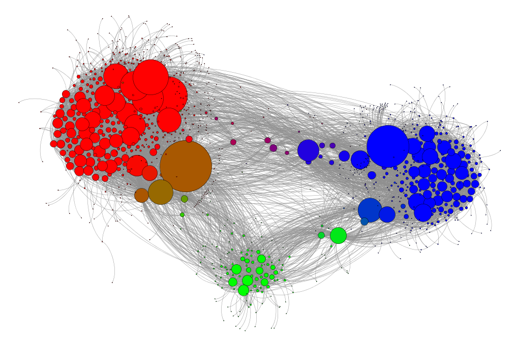
Figure 4: Graph sampled from the model with three latent communities, identified by colors red, green, blue. For each node, the intensity of each color is proportional to the value of the associated weight in that community. Pure red/green/blue color indicates the node is only strongly affiliated to a single community. A mixture of those colors indicates balanced affiliations to different communities. Graph generated with the software Gephi (Bastian et al., 2009).

The key component in our statistical network model is the multivariate Lévy measure ρ𝜌\rho in (8). Various approaches have been developed for constructing multivariate Lévy measures (Tankov, 2003; Cont and Tankov, 2003; Kallsen and Tankov, 2006; Barndorff-Nielsen et al., 2001; Skorohod, 1991), or more specifically vectors of completely random measures (Epifani and Lijoi, 2010; Leisen and Lijoi, 2011; Leisen et al., 2013; Griffin et al., 2013; Lijoi et al., 2014). We will in this paper consider the following particular form:

ρ(dw1,,dwp)=ek=1pγkwk0w0pF(dw1w0,,dwpw0)ρ0(dw0)𝜌𝑑subscript𝑤1𝑑subscript𝑤𝑝superscript𝑒superscriptsubscript𝑘1𝑝subscript𝛾𝑘subscript𝑤𝑘superscriptsubscript0superscriptsubscript𝑤0𝑝𝐹𝑑subscript𝑤1subscript𝑤0𝑑subscript𝑤𝑝subscript𝑤0subscript𝜌0𝑑subscript𝑤0\rho(dw_{1},\ldots,dw_{p})=e^{-\sum_{k=1}^{p}\gamma_{k}w_{k}}\int_{0}^{\infty}w_{0}^{-p}F\left(\frac{dw_{1}}{w_{0}},\ldots,\frac{dw_{p}}{w_{0}}\right)\rho_{0}(dw_{0}) (15)

where F(dβ1,dβp)𝐹𝑑subscript𝛽1𝑑subscript𝛽𝑝F(d\beta_{1},\ldots d\beta_{p}) is some score probability distribution on +dsuperscriptsubscript𝑑\mathbb{R}_{+}^{d}, with moment generating function M(t1,,tp)𝑀subscript𝑡1subscript𝑡𝑝M(t_{1},\ldots,t_{p}), ρ0subscript𝜌0\rho_{0} is a base Lévy measure on +subscript\mathbb{R}_{+} and γk0subscript𝛾𝑘0\gamma_{k}\geq 0 are exponentially tilting parameters for k=1,,p𝑘1𝑝k=1,\ldots,p. The model defined by (5) and (15) is a special case of the compound completely random measure (CCRM) model proposed by Griffin and Leisen (2017). It admits the following hierarchical construction, which makes interpretability, characterization of the conditionals and analysis of this class of models particularly easy. Let

W0=i=1wi0δθiCRM(ρ~0,λ)subscript𝑊0superscriptsubscript𝑖1subscript𝑤𝑖0subscript𝛿subscript𝜃𝑖similar-toCRMsubscript~𝜌0𝜆W_{0}=\sum_{i=1}^{\infty}w_{i0}\delta_{\theta_{i}}\sim\text{CRM}(\widetilde{\rho}_{0},\lambda) (16)

where ρ~0subscript~𝜌0\widetilde{\rho}_{0} is a measure on +subscript\mathbb{R}_{+} defined by ρ~0(dw0)=M(w0γ1,,w0γp)ρ0(dw0)subscript~𝜌0𝑑subscript𝑤0𝑀subscript𝑤0subscript𝛾1subscript𝑤0subscript𝛾𝑝subscript𝜌0𝑑subscript𝑤0\widetilde{\rho}_{0}(dw_{0})=M(-w_{0}\gamma_{1},\ldots,-w_{0}\gamma_{p})\rho_{0}(dw_{0}), and for k=1,,p𝑘1𝑝k=1,\ldots,p and i=1,2,𝑖12i=1,2,\ldots

wik=βikwi0subscript𝑤𝑖𝑘subscript𝛽𝑖𝑘subscript𝑤𝑖0w_{ik}=\beta_{ik}w_{i0}

where the scores βiksubscript𝛽𝑖𝑘\beta_{ik} have the following joint distribution

(βi1,,βip)|wi0indH(|wi0)(\beta_{i1},\ldots,\beta_{ip})|w_{i0}\overset{\text{ind}}{\sim}H(\cdot|w_{i0}) (17)

with H𝐻H is an exponentially tilted version of F𝐹F:

H(dβ1,,dβp|w0)=ew0k=1pγkβkF(dβ1,,dβp)+pew0k=1pγkβ~kF(dβ~1,,dβ~p).𝐻𝑑subscript𝛽1conditional𝑑subscript𝛽𝑝subscript𝑤0superscript𝑒subscript𝑤0superscriptsubscript𝑘1𝑝subscript𝛾𝑘subscript𝛽𝑘𝐹𝑑subscript𝛽1𝑑subscript𝛽𝑝subscriptsuperscriptsubscript𝑝superscript𝑒subscript𝑤0superscriptsubscript𝑘1𝑝subscript𝛾𝑘subscript~𝛽𝑘𝐹𝑑subscript~𝛽1𝑑subscript~𝛽𝑝H(d\beta_{1},\ldots,d\beta_{p}|w_{0})=\frac{e^{-w_{0}\sum_{k=1}^{p}\gamma_{k}\beta_{k}}F\left(d\beta_{1},\ldots,d\beta_{p}\right)}{\int_{\mathbb{R}_{+}^{p}}e^{-w_{0}\sum_{k=1}^{p}\gamma_{k}\widetilde{\beta}_{k}}F\left(d\widetilde{\beta}_{1},\ldots,d\widetilde{\beta}_{p}\right)}. (18)

Additionally, the set of points (wi0,βi1,,βip)i=1,2,subscriptsubscript𝑤𝑖0subscript𝛽𝑖1subscript𝛽𝑖𝑝𝑖12(w_{i0},\beta_{i1},\ldots,\beta_{ip})_{i=1,2,\ldots} is a Poisson point process with mean measure

ew0k=1pγkβkF(dβ1,,dβp)ρ0(dw0).superscript𝑒subscript𝑤0superscriptsubscript𝑘1𝑝subscript𝛾𝑘subscript𝛽𝑘𝐹𝑑subscript𝛽1𝑑subscript𝛽𝑝subscript𝜌0𝑑subscript𝑤0e^{-w_{0}\sum_{k=1}^{p}\gamma_{k}\beta_{k}}F(d\beta_{1},\ldots,d\beta_{p})\rho_{0}(dw_{0}). (19)

Dependence between the different CRMs is both tuned by the shared scaling parameter wi0subscript𝑤𝑖0w_{i0} and potential dependency between the scores (βi1,,βip)subscript𝛽𝑖1subscript𝛽𝑖𝑝(\beta_{i1},\ldots,\beta_{ip}). The hierarchical construction has the following interpretation:

  • The weight wi0subscript𝑤𝑖0w_{i0} is an individual scaling parameter for node i𝑖i whose distribution is tuned by the base Lévy measure ρ0subscript𝜌0\rho_{0}. It can be considered as a degree correction, as often used in network models (Karrer and Newman, 2011; Zhao et al., 2012; Herlau et al., 2015). As shown in Section 3, ρ0subscript𝜌0\rho_{0} tunes the overall sparsity properties of the network.

  • The community-related scores βiksubscript𝛽𝑖𝑘\beta_{ik} tune the level of affiliation of node i𝑖i to community k𝑘k; this is controlled by both the score distribution F𝐹F and the tilting coefficients γksubscript𝛾𝑘\gamma_{k}. These parameters tune the overlapping block-structure of the network.

An example of such a graph with three communities is displayed in Figure 4.

Specific choices for F𝐹F and ρ0subscript𝜌0\rho_{0}.

We now give here specific choices of score distribution F𝐹F and base Lévy measure ρ0subscript𝜌0\rho_{0}, which lead to scalable inference algorithms. As in Griffin and Leisen (2017), we consider that F𝐹F is a product of independent gamma distributions

F(dβ1,,dβp)=k=1pβkak1ebkβkbkakΓ(ak)dβk𝐹𝑑subscript𝛽1𝑑subscript𝛽𝑝superscriptsubscriptproduct𝑘1𝑝superscriptsubscript𝛽𝑘subscript𝑎𝑘1superscript𝑒subscript𝑏𝑘subscript𝛽𝑘superscriptsubscript𝑏𝑘subscript𝑎𝑘Γsubscript𝑎𝑘𝑑subscript𝛽𝑘F(d\beta_{1},\ldots,d\beta_{p})=\prod_{k=1}^{p}\beta_{k}^{a_{k}-1}e^{-b_{k}\beta_{k}}\frac{b_{k}^{a_{k}}}{\Gamma(a_{k})}d\beta_{k} (20)

where ak>0subscript𝑎𝑘0a_{k}>0,bk>0subscript𝑏𝑘0b_{k}>0, k=1,,p𝑘1𝑝k=1,\ldots,p, which leads to

H(dw1,,dwp|w0)k=1pwkak1ebkwkw0γkwkdwkproportional-to𝐻𝑑subscript𝑤1conditional𝑑subscript𝑤𝑝subscript𝑤0superscriptsubscriptproduct𝑘1𝑝superscriptsubscript𝑤𝑘subscript𝑎𝑘1superscript𝑒subscript𝑏𝑘subscript𝑤𝑘subscript𝑤0subscript𝛾𝑘subscript𝑤𝑘𝑑subscript𝑤𝑘H(dw_{1},\ldots,dw_{p}|w_{0})\propto\prod_{k=1}^{p}w_{k}^{a_{k}-1}e^{-\frac{b_{k}w_{k}}{w_{0}}-\gamma_{k}w_{k}}dw_{k}

which is also a product of gamma distributions.

ρ0subscript𝜌0\rho_{0} is set to be the mean measure of the jump part of a generalized gamma process (Hougaard, 1986; Brix, 1999), which has been extensively used in BNP models due to its generality, the interpretability of its parameters and its attractive conjugacy properties (James, 2002; Lijoi et al., 2007; Saeedi and Bouchard-Côté, 2011; Caron, 2012; Caron et al., 2014). The Lévy measure in this case is

ρ0(dw0)=1Γ(1σ)w01σexp(w0τ)dw0subscript𝜌0𝑑subscript𝑤01Γ1𝜎superscriptsubscript𝑤01𝜎subscript𝑤0𝜏𝑑subscript𝑤0\rho_{0}(dw_{0})=\frac{1}{\Gamma(1-\sigma)}w_{0}^{-1-\sigma}\exp(-w_{0}\tau)dw_{0} (21)

where the parameters (σ,τ)𝜎𝜏(\sigma,\tau) verify

σ(0,1),τ0 or σ(,0],τ>0.formulae-sequenceformulae-sequence𝜎01𝜏0 or 𝜎0𝜏0\displaystyle\sigma\in(0,1),\tau\geq 0~{}~{}\text{ or }~{}~{}\sigma\in(-\infty,0],\tau>0. (22)

The gamma process (σ=0𝜎0\sigma=0), the inverse Gaussian process (σ=12𝜎12\sigma=\frac{1}{2}) and the stable process (σ(0,1)𝜎01\sigma\in(0,1), τ=0𝜏0\tau=0) are special cases. Using (20) and (21), the multivariate Lévy measure has the following analytic form

ρ(dw1,,dwp)𝜌𝑑subscript𝑤1𝑑subscript𝑤𝑝\displaystyle\rho(dw_{1},\ldots,dw_{p}) =2ek=1pγkwkΓ(1σ)[k=1pwkak1bkakΓ(ak)](τk=1pbkwk)κ2Kκ(2τkbkwk)dw1dwpabsent2superscript𝑒superscriptsubscript𝑘1𝑝subscript𝛾𝑘subscript𝑤𝑘Γ1𝜎delimited-[]superscriptsubscriptproduct𝑘1𝑝superscriptsubscript𝑤𝑘subscript𝑎𝑘1superscriptsubscript𝑏𝑘subscript𝑎𝑘Γsubscript𝑎𝑘superscript𝜏superscriptsubscript𝑘1𝑝subscript𝑏𝑘subscript𝑤𝑘𝜅2subscript𝐾𝜅2𝜏subscript𝑘subscript𝑏𝑘subscript𝑤𝑘𝑑subscript𝑤1𝑑subscript𝑤𝑝\displaystyle=\frac{2e^{-\sum_{k=1}^{p}\gamma_{k}w_{k}}}{\Gamma(1-\sigma)}\left[\prod_{k=1}^{p}\frac{w_{k}^{a_{k}-1}b_{k}^{a_{k}}}{\Gamma(a_{k})}\right]\left(\frac{\tau}{\sum_{k=1}^{p}b_{k}w_{k}}\right)^{{-}\frac{\kappa}{2}}K_{\kappa}\left(2\sqrt{\tau\sum_{k}b_{k}w_{k}}\right)dw_{1}\ldots dw_{p}

where κ=σ+k=1pak𝜅𝜎superscriptsubscript𝑘1𝑝subscript𝑎𝑘\kappa=\sigma+\sum_{k=1}^{p}a_{k} and K𝐾K is the modified Bessel function of the second kind.

3 Properties and Simulation

The first theorem provides expressions for the expected number of edges in the multigraph and simple graph, and for the expected number of nodes. The proof is given in Appendix C.

Theorem 3

The expected number of edges in the multigraph Dαsubscriptsuperscript𝐷𝛼D^{*}_{\alpha}, edges in the undirected graph Nα(e)subscriptsuperscript𝑁𝑒𝛼N^{(e)}_{\alpha} and observed nodes Nαsubscript𝑁𝛼N_{\alpha} are given as follows:

𝔼[Dα]𝔼delimited-[]subscriptsuperscript𝐷𝛼\displaystyle\mathbb{E}[D^{*}_{\alpha}] =α2μTμ+αtr(Σ)absentsuperscript𝛼2superscript𝜇𝑇𝜇𝛼trΣ\displaystyle=\alpha^{2}\mu^{T}\mu+\alpha\text{tr}(\Sigma)
𝔼[Nα(e)]𝔼delimited-[]subscriptsuperscript𝑁𝑒𝛼\displaystyle\mathbb{E}[N^{(e)}_{\alpha}] =α+p(1ewTw)ρ(dw1,,dwp)+α22+pψ(2w1,,2wp)ρ(dw1,,dwp)absent𝛼subscriptsubscriptsuperscript𝑝1superscript𝑒superscript𝑤𝑇𝑤𝜌𝑑subscript𝑤1𝑑subscript𝑤𝑝superscript𝛼22subscriptsubscriptsuperscript𝑝𝜓2subscript𝑤12subscript𝑤𝑝𝜌𝑑subscript𝑤1𝑑subscript𝑤𝑝\displaystyle=\alpha\int_{\mathbb{R}^{p}_{+}}\left(1-e^{-w^{T}w}\right)\rho(dw_{1},\ldots,dw_{p})+\frac{\alpha^{2}}{2}\int_{\mathbb{R}^{p}_{+}}\psi(2w_{1},\ldots,2w_{p})\rho(dw_{1},\ldots,dw_{p})
𝔼[Nα]𝔼delimited-[]subscript𝑁𝛼\displaystyle\mathbb{E}[N_{\alpha}] =α+p(1ewTwαψ(2w))ρ(dw1,,dwp)absent𝛼subscriptsubscriptsuperscript𝑝1superscript𝑒superscript𝑤𝑇𝑤𝛼𝜓2𝑤𝜌𝑑subscript𝑤1𝑑subscript𝑤𝑝\displaystyle=\alpha\int_{\mathbb{R}^{p}_{+}}\left(1-e^{-w^{T}w-\alpha\psi(2w)}\right)\rho(dw_{1},\ldots,dw_{p})

where μ=+pwρ(dw1,,dwp)𝜇subscriptsubscriptsuperscript𝑝𝑤𝜌𝑑subscript𝑤1𝑑subscript𝑤𝑝\mu=\int_{\mathbb{R}^{p}_{+}}w\rho(dw_{1},\ldots,dw_{p}), Σ=+pwwTρ(dw1,,dwp)Σsubscriptsubscriptsuperscript𝑝𝑤superscript𝑤𝑇𝜌𝑑subscript𝑤1𝑑subscript𝑤𝑝\Sigma=\int_{\mathbb{R}^{p}_{+}}ww^{T}\rho(dw_{1},\ldots,dw_{p}) and ψ(t1,,tp)=+p(1ek=1ptiwi)ρ(dw1,,dwp)𝜓subscript𝑡1subscript𝑡𝑝subscriptsubscriptsuperscript𝑝1superscript𝑒superscriptsubscript𝑘1𝑝subscript𝑡𝑖subscript𝑤𝑖𝜌𝑑subscript𝑤1𝑑subscript𝑤𝑝\psi(t_{1},\ldots,t_{p})=\int_{\mathbb{R}^{p}_{+}}(1-e^{-\sum_{k=1}^{p}t_{i}w_{i}})\rho(dw_{1},\ldots,dw_{p}) is the multivariable Laplace exponent.

3.1 Exchangeability

The point process Z𝑍Z defined by (11) is jointly exchangeable in the sense of Kallenberg (1990, 2005). For any h>00h>0 and any permutation π𝜋\pi of \mathbb{N}

(Z(Ai×Aj))=𝑑(Z(Aπ(i)×Aπ(j))) for (i,j)2𝑍subscript𝐴𝑖subscript𝐴𝑗𝑑𝑍subscript𝐴𝜋𝑖subscript𝐴𝜋𝑗 for 𝑖𝑗superscript2(Z(A_{i}\times A_{j}))\overset{d}{=}(Z(A_{\pi(i)}\times A_{\pi(j)}))\text{ for }(i,j)\in\mathbb{N}^{2} (23)

where Ai=[h(i1),hi]subscript𝐴𝑖𝑖1𝑖A_{i}=[h(i-1),hi]. This follows directly from the fact that the vector of CRMs (W1,,Wp)subscript𝑊1subscript𝑊𝑝(W_{1},\ldots,W_{p}) has independent and identically distributed increments, hence

(W1(Ai),,Wp(Ai))=𝑑(W1(Aπ(i)),,Wp(Aπ(i))).subscript𝑊1subscript𝐴𝑖subscript𝑊𝑝subscript𝐴𝑖𝑑subscript𝑊1subscript𝐴𝜋𝑖subscript𝑊𝑝subscript𝐴𝜋𝑖(W_{1}(A_{i}),\ldots,W_{p}(A_{i}))\overset{d}{=}(W_{1}(A_{\pi(i)}),\ldots,W_{p}(A_{\pi(i)})). (24)

The model thus falls into the general representation theorem for exchangeable point processes (Kallenberg, 1990).

3.2 Sparsity

In this section, following the asymptotic notations of Janson (2011), we derive the sparsity properties of our graph model, first for the general construction of Section 2.1, then for the specific construction on compound CRMs of Section 2.2. Similarly to the notations in Caron and Fox (2017), let Zαsubscript𝑍𝛼Z_{\alpha} be the restriction of Z𝑍Z to the box [0,α]2superscript0𝛼2[0,\alpha]^{2}. Let (Nα)α0subscriptsubscript𝑁𝛼𝛼0(N_{\alpha})_{\alpha\geq 0} and (Nα(e))α0subscriptsuperscriptsubscript𝑁𝛼𝑒𝛼0(N_{\alpha}^{(e)})_{\alpha\geq 0} be counting processes respectively corresponding to the number of nodes and edges in Zαsubscript𝑍𝛼Z_{\alpha}:

Nαsubscript𝑁𝛼\displaystyle N_{\alpha} =i𝟙θiα𝟙(jzij𝟙θjα)1absentsubscript𝑖subscript1subscript𝜃𝑖𝛼subscript1subscript𝑗subscript𝑧𝑖𝑗subscript1subscript𝜃𝑗𝛼1\displaystyle=\sum_{i}\mathds{1}_{\theta_{i}\leq\alpha}\mathds{1}_{(\sum_{j}z_{ij}\mathds{1}_{\theta_{j}\leq\alpha})\geq 1}
Nα(e)superscriptsubscript𝑁𝛼𝑒\displaystyle N_{\alpha}^{(e)} =ijzij𝟙θiα𝟙θjα.absentsubscript𝑖𝑗subscript𝑧𝑖𝑗subscript1subscript𝜃𝑖𝛼subscript1subscript𝜃𝑗𝛼\displaystyle=\sum_{i\leq j}z_{ij}\mathds{1}_{\theta_{i}\leq\alpha}\mathds{1}_{\theta_{j}\leq\alpha}.

Note that in the propositions below, we discard the trivial case +pρ(dw1,,dwp)=0subscriptsubscriptsuperscript𝑝𝜌𝑑subscript𝑤1𝑑subscript𝑤𝑝0\int_{\mathbb{R}^{p}_{+}}\rho(dw_{1},\ldots,dw_{p})=0 which implies Nα(e)=Nα=0superscriptsubscript𝑁𝛼𝑒subscript𝑁𝛼0N_{\alpha}^{(e)}=N_{\alpha}=0 a.s.

General construction.

The next proposition characterizes the sparsity properties of the random graph depending on the properties of the Lévy measure ρ𝜌\rho. In particular, if

+pρ(dw1,,dwp)=subscriptsubscriptsuperscript𝑝𝜌𝑑subscript𝑤1𝑑subscript𝑤𝑝\int_{\mathbb{R}^{p}_{+}}\rho(dw_{1},\ldots,dw_{p})=\infty (25)

then, for any α>0𝛼0\alpha>0, there is a.s. an infinite number of θi[0,α]subscript𝜃𝑖0𝛼\theta_{i}\in[0,\alpha] for which kwik>0subscript𝑘subscript𝑤𝑖𝑘0\sum_{k}w_{ik}>0 and the vector of CRMs is called infinite-activity. Otherwise, it is finite-activity.

Proposition 4

Assume that, for any k=1,,p𝑘1𝑝k=1,\ldots,p,

+pwkρ(dw1,,dwp)<subscriptsubscriptsuperscript𝑝subscript𝑤𝑘𝜌𝑑subscript𝑤1𝑑subscript𝑤𝑝\int_{{\mathbb{R}^{p}_{+}}}w_{k}\rho(dw_{1},\ldots,dw_{p})<\infty (26)

Then

Nα(e)={Θ(Nα2)if (W1,,Wp) is finite-activityo(Nα2)otherwisesuperscriptsubscript𝑁𝛼𝑒casesΘsuperscriptsubscript𝑁𝛼2if subscript𝑊1subscript𝑊𝑝 is finite-activity𝑜superscriptsubscript𝑁𝛼2otherwiseN_{\alpha}^{(e)}=\left\{\begin{array}[]{ll}\Theta(N_{\alpha}^{2})&\text{if }(W_{1},\ldots,W_{p})\text{ is finite-activity}\\ o(N_{\alpha}^{2})&\text{otherwise}\end{array}\right.

a.s. as α𝛼\alpha tends to \infty.

The proof is given in Appendix B.

Construction based on CCRMs.

For the CCRM Lévy measure (15), the sparsity properties are solely tuned by the base Lévy measure ρ0subscript𝜌0\rho_{0}. Ignoring trivial degenerate cases for the score distribution F𝐹F, it is easily shown that the CCRM model defined by (5) and (15) is infinite-activity iff the Lévy measure ρ0subscript𝜌0\rho_{0} verifies

0ρ0(dw)=.superscriptsubscript0subscript𝜌0𝑑𝑤\int_{0}^{\infty}\rho_{0}(dw)=\infty. (27)

In this case all CRMs W0,W1,,Wpsubscript𝑊0subscript𝑊1subscript𝑊𝑝W_{0},W_{1},\ldots,W_{p} are infinite-activity. Otherwise they are all finite-activity and the vector of CRMs is finite-activity. In the particular case of a CCRM with independent gamma distributed scores (20) and generalized gamma process base measure (21), the condition (27) is satisfied whenever σ0𝜎0\sigma\geq 0. The next proposition characterizes the sparsity of the network depending on the properties of the base Lévy measure ρ0subscript𝜌0\rho_{0}.

Proposition 5

Assume that

0w0ρ0(dw0)<superscriptsubscript0subscript𝑤0subscript𝜌0𝑑subscript𝑤0\int_{0}^{\infty}w_{0}\rho_{0}(dw_{0})<\infty (28)

and F𝐹F is not degenerated at 0. Then

Nα(e)={Θ(Nα2)if 0ρ0(dw)<o(Nα2)otherwisesuperscriptsubscript𝑁𝛼𝑒casesΘsuperscriptsubscript𝑁𝛼2if superscriptsubscript0subscript𝜌0𝑑𝑤𝑜superscriptsubscript𝑁𝛼2otherwiseN_{\alpha}^{(e)}=\left\{\begin{array}[]{ll}\Theta(N_{\alpha}^{2})&\text{if }\int_{0}^{\infty}\rho_{0}(dw)<\infty\\ o(N_{\alpha}^{2})&\text{otherwise}\end{array}\right.

a.s. as α𝛼\alpha tends to \infty. Furthermore, if the tail Lévy intensity ρ¯0subscript¯𝜌0\overline{\rho}_{0} defined by

ρ¯0(x)=xρ0(dw),subscript¯𝜌0𝑥superscriptsubscript𝑥subscript𝜌0𝑑𝑤\overline{\rho}_{0}(x)=\int_{x}^{\infty}\rho_{0}(dw), (29)

is a regularly varying function, i.e.

ρ¯0(x)xσ(1/x)1 as x0subscript¯𝜌0𝑥superscript𝑥𝜎1𝑥1 as 𝑥0\frac{\overline{\rho}_{0}(x)}{x^{-\sigma}\ell(1/x)}\longrightarrow 1\text{ as }x\rightarrow 0

for some σ(0,1)𝜎01\sigma\in(0,1) where \ell is a slowly varying function verifying limt(at)/(t)=1subscript𝑡𝑎𝑡𝑡1\lim_{t\rightarrow\infty}\ell(at)/\ell(t)=1 for any a>0𝑎0a>0 and limt(t)>0subscript𝑡𝑡0\lim_{t\rightarrow\infty}\ell(t)>0, then

Nα(e)=O(Nα2/(1+σ))superscriptsubscript𝑁𝛼𝑒𝑂superscriptsubscript𝑁𝛼21𝜎N_{\alpha}^{(e)}=O(N_{\alpha}^{2/(1+\sigma)})

a.s. as α𝛼\alpha tends to \infty. In the particular case of a CCRM with independent gamma distributed scores (20) and generalized gamma process base measure (21), condition (28) is equivalent to having τ>0𝜏0\tau>0. In this case, we therefore have

Nα(e)={Θ(Nα2)if σ<0o(Nα2)if σ0O(Nα2/(1+σ))if σ(0,1).superscriptsubscript𝑁𝛼𝑒casesΘsuperscriptsubscript𝑁𝛼2if 𝜎0𝑜superscriptsubscript𝑁𝛼2if 𝜎0𝑂superscriptsubscript𝑁𝛼21𝜎if 𝜎01N_{\alpha}^{(e)}=\left\{\begin{array}[]{ll}\Theta(N_{\alpha}^{2})&\text{if }\sigma<0\\ o(N_{\alpha}^{2})&\text{if }\sigma\geq 0\\ O(N_{\alpha}^{2/(1+\sigma)})&\text{if }\sigma\in(0,1).\end{array}\right.
Refer to caption
Refer to caption
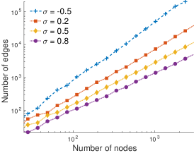
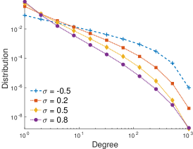
Figure 5: Empirical analysis of the properties of CCRM based graphs generated with parameters p=2𝑝2p=2, τ=1𝜏1\tau=1, ak=0.2subscript𝑎𝑘0.2a_{k}=0.2, bk=1psubscript𝑏𝑘1𝑝b_{k}=\frac{1}{p} and averaging over various α𝛼\alpha. (a) Number of edges versus the number of nodes and (b) degree distributions on a log-log scale for various σ𝜎\sigma: one finite-activity CCRM (σ=0.5𝜎0.5\sigma=-0.5) and three infinite-activity CCRMs (σ=0.2𝜎0.2\sigma=0.2, σ=0.5𝜎0.5\sigma=0.5 and σ=0.8𝜎0.8\sigma=0.8). In (a) we note growth at a rate Θ(Nα2)Θsuperscriptsubscript𝑁𝛼2\Theta(N_{\alpha}^{2}) for σ=0.5𝜎0.5\sigma=-0.5 and O(Nα2/(1+σ))𝑂superscriptsubscript𝑁𝛼21𝜎O(N_{\alpha}^{2/(1+\sigma)}) for σ(0,1)𝜎01\sigma\in(0,1).

The proof is given in Appendix B. Figure 5(a) provides an empirical illustration of Proposition 5 for a CCRM with independent gamma scores and generalized gamma based Lévy measure. Figure 5(b) shows empirically that the degree distribution also exhibits a power-law behaviour when σ(0,1)𝜎01\sigma\in(0,1).

3.3 Simulation

The point process Z𝑍Z is defined on the plane. We describe in this section how to sample realizations of restrictions Zαsubscript𝑍𝛼Z_{\alpha} of Z𝑍Z to the box [0,α]2superscript0𝛼2[0,\alpha]^{2}.

General construction.

The hierarchical construction given by Eq. (11) suggests a direct way to sample from the model:

  1. 1.

    Sample (wi1,,wip,θi)i=1,2,subscriptsubscript𝑤𝑖1subscript𝑤𝑖𝑝subscript𝜃𝑖𝑖12(w_{i1},\ldots,w_{ip},\theta_{i})_{i=1,2,\ldots} from a Poisson process with mean measure ν(dw1,,dwp,dθ)𝟙θ[0,α]𝜈𝑑subscript𝑤1𝑑subscript𝑤𝑝𝑑𝜃subscript1𝜃0𝛼\nu(dw_{1},\ldots,dw_{p},d\theta){\mathds{1}}_{\theta\in[0,\alpha]}.

  2. 2.

    For each pair of points, sample zijsubscript𝑧𝑖𝑗z_{ij} from (14).

There are two caveats to this strategy. First, for infinite-activity CRMs, the number of points in +p×[0,α]superscriptsubscript𝑝0𝛼\mathbb{R}_{+}^{p}\times[0,\alpha] is almost surely infinite; even for finite-activity CRMs, it may be so large that it is not practically feasible. We need therefore to resort to an approximation, by sampling from a Poisson process with an approximate mean measure νε(dw1,,dwp,dθ)𝟙θ[0,α]=ρε(dw1,,dwp)λ(dθ)𝟙θ[0,α]superscript𝜈𝜀𝑑subscript𝑤1𝑑subscript𝑤𝑝𝑑𝜃subscript1𝜃0𝛼superscript𝜌𝜀𝑑subscript𝑤1𝑑subscript𝑤𝑝𝜆𝑑𝜃subscript1𝜃0𝛼\nu^{\varepsilon}(dw_{1},\ldots,dw_{p},d\theta){\mathds{1}}_{\theta\in[0,\alpha]}=\rho^{\varepsilon}(dw_{1},\ldots,dw_{p})\lambda(d\theta){\mathds{1}}_{\theta\in[0,\alpha]} where

+pρε(dw1,,dwp)<subscriptsuperscriptsubscript𝑝superscript𝜌𝜀𝑑subscript𝑤1𝑑subscript𝑤𝑝\int_{\mathbb{R}_{+}^{p}}\rho^{\varepsilon}(dw_{1},\ldots,dw_{p})<\infty

with ε>0𝜀0\varepsilon>0 controlling the level of approximation. The approximation is specific to the choice of the mean measure, and we describe such an approximation for CCRMs below.

The second caveat is that, for applying Eq. (14), we need to consider all pairs ij𝑖𝑗i\leq j, which can be computationally problematic. We can instead, similarly to Caron and Fox (2017), use the hierarchical Poisson construction as follows:

  1. 1.

    Sample (wi1,,wip,θi)i=1,2,,Ksubscriptsubscript𝑤𝑖1subscript𝑤𝑖𝑝subscript𝜃𝑖𝑖12𝐾(w_{i1},\ldots,w_{ip},\theta_{i})_{i=1,2,\ldots,K} from a Poisson process with mean measure νε(dw1,,dwp,dθ)𝟙θ[0,α]superscript𝜈𝜀𝑑subscript𝑤1𝑑subscript𝑤𝑝𝑑𝜃subscript1𝜃0𝛼\nu^{\varepsilon}(dw_{1},\ldots,dw_{p},d\theta){\mathds{1}}_{\theta\in[0,\alpha]}. Let Wk,αε=i=1Kwikδθisuperscriptsubscript𝑊𝑘𝛼𝜀superscriptsubscript𝑖1𝐾subscript𝑤𝑖𝑘subscript𝛿subscript𝜃𝑖W_{k,\alpha}^{\varepsilon}=\sum_{i=1}^{K}w_{ik}\delta_{\theta_{i}} be the associated truncated CRMs and Wk,αε=i=1Kwiksuperscriptsubscript𝑊𝑘𝛼𝜀superscriptsubscript𝑖1𝐾subscript𝑤𝑖𝑘W_{k,\alpha}^{\varepsilon\ast}=\sum_{i=1}^{K}w_{ik} their total masses.

  2. 2.

    For k=1,,p𝑘1𝑝k=1,\ldots,p, sample Dk,α|Wk,αεPoisson((Wk,αε)2)similar-toconditionalsubscriptsuperscript𝐷𝑘𝛼superscriptsubscript𝑊𝑘𝛼𝜀Poissonsuperscriptsuperscriptsubscript𝑊𝑘𝛼𝜀2D^{\ast}_{k,\alpha}|W_{k,\alpha}^{\varepsilon\ast}\sim\text{Poisson}((W_{k,\alpha}^{\varepsilon\ast})^{2}).

  3. 3.

    For k=1,,p𝑘1𝑝k=1,\ldots,p, =1,,Dk,α1subscriptsuperscript𝐷𝑘𝛼\ell=1,\ldots,D^{\ast}_{k,\alpha}, j=1,2𝑗12j=1,2, sample Ukj|Wk,αεindWk,αεWk,αεconditionalsubscript𝑈𝑘𝑗superscriptsubscript𝑊𝑘𝛼𝜀indsimilar-tosuperscriptsubscript𝑊𝑘𝛼𝜀superscriptsubscript𝑊𝑘𝛼𝜀U_{k\ell j}|W_{k,\alpha}^{\varepsilon}\overset{\text{ind}}{\sim}\frac{W_{k,\alpha}^{\varepsilon}}{W_{k,\alpha}^{\varepsilon\ast}}.

  4. 4.

    Set Dk,αε==1Dk,αδUk1,k2superscriptsubscript𝐷𝑘𝛼𝜀superscriptsubscript1subscriptsuperscript𝐷𝑘𝛼subscript𝛿subscript𝑈𝑘1𝑘2D_{k,\alpha}^{\varepsilon}=\sum_{\ell=1}^{D^{\ast}_{k,\alpha}}\delta_{U_{k\ell 1,k\ell 2}}.

  5. 5.

    Obtain Z𝑍Z from (D1,,Dp)subscript𝐷1subscript𝐷𝑝(D_{1},\ldots,D_{p}) as in (11).

Construction based on CCRMs.

The hierarchical construction of compound CRMs suggests an algorithm to simulate a vector of CRMS. We consider the following (truncated) mean measure

ρε(dw1,,dwp)=ek=1pγkwkεw0pF(dw1w0,,dwpw0)ρ0(dw0)superscript𝜌𝜀𝑑subscript𝑤1𝑑subscript𝑤𝑝superscript𝑒superscriptsubscript𝑘1𝑝subscript𝛾𝑘subscript𝑤𝑘superscriptsubscript𝜀superscriptsubscript𝑤0𝑝𝐹𝑑subscript𝑤1subscript𝑤0𝑑subscript𝑤𝑝subscript𝑤0subscript𝜌0𝑑subscript𝑤0\rho^{\varepsilon}(dw_{1},\ldots,dw_{p})=e^{-\sum_{k=1}^{p}\gamma_{k}w_{k}}\int_{\varepsilon}^{\infty}w_{0}^{-p}F\left(\frac{dw_{1}}{w_{0}},\ldots,\frac{dw_{p}}{w_{0}}\right)\rho_{0}(dw_{0}) (30)

with ε0𝜀0\varepsilon\geq 0. We can sample from the (truncated) CCRM as follows

  1. 1.

    (a) Sample (wi0,θi)i=1,,Ksubscriptsubscript𝑤𝑖0subscript𝜃𝑖𝑖1𝐾(w_{i0},\theta_{i})_{i=1,\ldots,K} from a Poisson point process with mean measure ρ~0(dw0)λ(dθ)𝟙{w0>ε,θ[0,α]}subscript~𝜌0𝑑subscript𝑤0𝜆𝑑𝜃subscript1formulae-sequencesubscript𝑤0𝜀𝜃0𝛼\widetilde{\rho}_{0}(dw_{0})\lambda(d\theta){\mathds{1}}_{\{w_{0}>\varepsilon,\theta\in[0,\alpha]\}}.

  2.   

    (b) For i=1,,K𝑖1𝐾i=1,\ldots,K and k=1,,p𝑘1𝑝k=1,\ldots,p, set wik=βikwi0subscript𝑤𝑖𝑘subscript𝛽𝑖𝑘subscript𝑤𝑖0w_{ik}=\beta_{ik}w_{i0} where (βi1,,βip)|wi0conditionalsubscript𝛽𝑖1subscript𝛽𝑖𝑝subscript𝑤𝑖0(\beta_{i1},\ldots,\beta_{ip})|w_{i0} is drawn from (17).

The truncation level ε𝜀\varepsilon is set to 0 for finite-activity CCRMs, and ε>0𝜀0\varepsilon>0 otherwise. We explain in Appendix D how to perform step 1.(a) in the case of a tilted generalized gamma process.

4 Posterior inference

In this section, we describe a MCMC algorithm for posterior inference of the model parameters and hyperparameters in the statistical network model defined in Section 2. We first describe the data augmentation scheme and characterization of conditionals. We then describe the sampler for a general Lévy measure ρ𝜌\rho, and finally derive the sampler for compound CRMs.

4.1 Characterization of conditionals and data augmentation

Assume that we have observed a set of connections (zij)1i,jNαsubscriptsubscript𝑧𝑖𝑗formulae-sequence1𝑖𝑗subscript𝑁𝛼(z_{ij})_{1\leq i,j\leq N_{\alpha}}, where Nαsubscript𝑁𝛼N_{\alpha} is the number of nodes with at least one connection. We aim at inferring the positive parameters (wi1,,wip)i=1,,Nαsubscriptsubscript𝑤𝑖1subscript𝑤𝑖𝑝𝑖1subscript𝑁𝛼(w_{i1},\ldots,w_{ip})_{i=1,\ldots,N_{\alpha}} associated to the nodes with at least one connection. We also want to estimate the positive parameters associated to the other nodes with no connection. The number of such nodes may be large, and even infinite for infinite-activity CRMs; but under our model, these parameters are only identifiable through their sum, denoted (w1,,wp)subscript𝑤absent1subscript𝑤absent𝑝(w_{\ast 1},\ldots,w_{\ast p}). Note that the node locations θisubscript𝜃𝑖\theta_{i} are not likelihood identifiable, and we will not try to infer them. We assume that there is a set of unknown hyperparameters ϕitalic-ϕ\phi of the mean intensity ρ𝜌\rho, with prior p(ϕ)𝑝italic-ϕp(\phi). We assume that the Lévy measure ρ𝜌\rho is absolutely continuous with respect to the Lebesgue measure on dsuperscript𝑑\mathbb{R}^{d}, and write simply ρ(dw1,,dwp;ϕ)=ρ(w1,,wp;ϕ)dw1dwp𝜌𝑑subscript𝑤1𝑑subscript𝑤𝑝italic-ϕ𝜌subscript𝑤1subscript𝑤𝑝italic-ϕ𝑑subscript𝑤1𝑑subscript𝑤𝑝\rho(dw_{1},\ldots,dw_{p};\phi)=\rho(w_{1},\ldots,w_{p};\phi)dw_{1}\ldots dw_{p}. The parameter α𝛼\alpha is also assumed to be unknown, with some prior αGamma(aα,bα)similar-to𝛼Gammasubscript𝑎𝛼subscript𝑏𝛼\alpha\sim\operatorname{Gamma}(a_{\alpha},b_{\alpha}) with aα>0,bα>0formulae-sequencesubscript𝑎𝛼0subscript𝑏𝛼0a_{\alpha}>0,b_{\alpha}>0. We therefore aim at approximating p((w1k,,wNαk,wk)k=1,,p,ϕ,α|(zij)1i,jNα)𝑝subscriptsubscript𝑤1𝑘subscript𝑤subscript𝑁𝛼𝑘subscript𝑤absent𝑘𝑘1𝑝italic-ϕconditional𝛼subscriptsubscript𝑧𝑖𝑗formulae-sequence1𝑖𝑗subscript𝑁𝛼p((w_{1k},\ldots,w_{N_{\alpha}k},w_{\ast k})_{k=1,\ldots,p},\phi,\alpha|(z_{ij})_{1\leq i,j\leq N_{\alpha}}).

As a first step, we characterize the conditional distribution of the restricted vector of CRMs (W1α,,Wpα)subscript𝑊1𝛼subscript𝑊𝑝𝛼(W_{1\alpha},\ldots,W_{p\alpha}) given the restricted measures (D1α,,Dpα)subscript𝐷1𝛼subscript𝐷𝑝𝛼(D_{1\alpha},\ldots,D_{p\alpha}). Proposition 6 below extends Theorem 12 in Caron and Fox (2017) to the multivariate setting.

Proposition 6

Let (θ1,,θNα)subscript𝜃1subscript𝜃subscript𝑁𝛼(\theta_{1},\ldots,\theta_{N_{\alpha}}), Nα0subscript𝑁𝛼0N_{\alpha}\geq 0 be the support points of (D1α,,Dpα)subscript𝐷1𝛼subscript𝐷𝑝𝛼(D_{1\alpha},\ldots,D_{p\alpha}), with

Dkα=1i,jNαnijkδ(θi,θj).subscript𝐷𝑘𝛼subscriptformulae-sequence1𝑖𝑗subscript𝑁𝛼subscript𝑛𝑖𝑗𝑘subscript𝛿subscript𝜃𝑖subscript𝜃𝑗D_{k\alpha}=\sum_{1\leq i,j\leq N_{\alpha}}n_{ijk}\delta_{(\theta_{i},\theta_{j})}.

The conditional distribution of (W1α,,Wpα)subscript𝑊1𝛼subscript𝑊𝑝𝛼(W_{1\alpha},\ldots,W_{p\alpha}) given (D1α,,Dpα)subscript𝐷1𝛼subscript𝐷𝑝𝛼(D_{1\alpha},\ldots,D_{p\alpha}) is equivalent to the distribution of

(W~1+i=1Nαwi1δθi,,W~p+i=1Nαwipδθi)subscript~𝑊1superscriptsubscript𝑖1subscript𝑁𝛼subscript𝑤𝑖1subscript𝛿subscript𝜃𝑖subscript~𝑊𝑝superscriptsubscript𝑖1subscript𝑁𝛼subscript𝑤𝑖𝑝subscript𝛿subscript𝜃𝑖\left(\widetilde{W}_{1}+\sum_{i=1}^{N_{\alpha}}w_{i1}\delta_{\theta_{i}},\ldots,\widetilde{W}_{p}+\sum_{i=1}^{N_{\alpha}}w_{ip}\delta_{\theta_{i}}\right) (31)

where (W~1,,W~p)subscript~𝑊1subscript~𝑊𝑝(\widetilde{W}_{1},\ldots,\widetilde{W}_{p}) is a vector of discrete random measures, which depends on (D1α,,Dpα)subscript𝐷1𝛼subscript𝐷𝑝𝛼(D_{1\alpha},\ldots,D_{p\alpha}) only through the total masses wk=W~k([0,α])subscript𝑤absent𝑘subscript~𝑊𝑘0𝛼w_{\ast k}=\widetilde{W}_{k}([0,\alpha]).

The set of weights (wik)i=1,,Nα;k=1,,psubscriptsubscript𝑤𝑖𝑘formulae-sequence𝑖1subscript𝑁𝛼𝑘1𝑝(w_{ik})_{i=1,\ldots,N_{\alpha};k=1,\ldots,p} and (wk)k=1,,psubscriptsubscript𝑤absent𝑘𝑘1𝑝(w_{\ast k})_{k=1,\ldots,p} are dependent, with joint conditional distribution

p((w1k,,wNαk,wk)k=1,,p|(nijk)1i,jNα;k=1,,p,ϕ,α)𝑝conditionalsubscriptsubscript𝑤1𝑘subscript𝑤subscript𝑁𝛼𝑘subscript𝑤absent𝑘𝑘1𝑝subscriptsubscript𝑛𝑖𝑗𝑘formulae-sequence1𝑖formulae-sequence𝑗subscript𝑁𝛼𝑘1𝑝italic-ϕ𝛼\displaystyle p((w_{1k},\ldots,w_{N_{\alpha}k},w_{\ast k})_{k=1,\ldots,p}|(n_{ijk})_{1\leq i,j\leq N_{\alpha}{;}k=1,\ldots,p},\phi,\alpha)
[i=1Nαk=1pwikmik]ek=1p(wk+i=1Nαwik)2[i=1Nαρ(wi1,,wip;ϕ)]αNαgα(w1,,wp;ϕ)proportional-toabsentdelimited-[]superscriptsubscriptproduct𝑖1subscript𝑁𝛼superscriptsubscriptproduct𝑘1𝑝superscriptsubscript𝑤𝑖𝑘subscript𝑚𝑖𝑘superscript𝑒superscriptsubscript𝑘1𝑝superscriptsubscript𝑤absent𝑘superscriptsubscript𝑖1subscript𝑁𝛼subscript𝑤𝑖𝑘2delimited-[]superscriptsubscriptproduct𝑖1subscript𝑁𝛼𝜌subscript𝑤𝑖1subscript𝑤𝑖𝑝italic-ϕsuperscript𝛼subscript𝑁𝛼subscript𝑔absent𝛼subscript𝑤absent1subscript𝑤absent𝑝italic-ϕ\displaystyle~{}~{}~{}~{}\propto\left[\prod_{i=1}^{N_{\alpha}}\prod_{k=1}^{p}w_{ik}^{m_{ik}}\right]e^{-\sum_{k=1}^{p}(w_{\ast k}+\sum_{i=1}^{N_{\alpha}}w_{ik})^{2}}\left[\prod_{i=1}^{N_{\alpha}}\rho(w_{i1},\ldots,w_{ip};\phi)\right]\alpha^{N_{\alpha}}g_{\ast\alpha}(w_{\ast 1},\ldots,w_{\ast p};\phi) (32)

where mik=j=1Nαnijk+njiksubscript𝑚𝑖𝑘superscriptsubscript𝑗1subscript𝑁𝛼subscript𝑛𝑖𝑗𝑘subscript𝑛𝑗𝑖𝑘m_{ik}=\sum_{j=1}^{N_{\alpha}}n_{ijk}+n_{jik} and gα(w1,,wp;ϕ)subscript𝑔absent𝛼subscript𝑤absent1subscript𝑤absent𝑝italic-ϕg_{\ast\alpha}(w_{\ast 1},\ldots,w_{\ast p};\phi) is the probability density function of the random vector (W1([0,α]),,Wp([0,α]))subscript𝑊10𝛼subscript𝑊𝑝0𝛼(W_{1}([0,\alpha]),\ldots,W_{p}([0,\alpha])).

The proof can be straightforwardly adapted from that of Caron and Fox (2017), or from Proposition 5.2 of James (2014) and is omitted here. It builds on other posterior characterizations in Bayesian nonparametric models (Prünster, 2002; James, 2002, 2005; James et al., 2009).

Data augmentation.

Similarly to Caron and Fox (2017), we introduce latent count variables n~ijk=nijk+njiksubscript~𝑛𝑖𝑗𝑘subscript𝑛𝑖𝑗𝑘subscript𝑛𝑗𝑖𝑘\widetilde{n}_{ijk}=n_{ijk}+n_{jik} with

(n~ij1,,n~ijp)|w,zconditionalsubscript~𝑛𝑖𝑗1subscript~𝑛𝑖𝑗𝑝𝑤𝑧\displaystyle(\widetilde{n}_{ij1},\ldots,\widetilde{n}_{ijp})|w,z {δ(0,,0)if zij=0tPoisson(2wi1wj1,,2wipwjp)if zij=1ijsimilar-toabsentcasessubscript𝛿00if subscript𝑧𝑖𝑗0tPoisson2subscript𝑤𝑖1subscript𝑤𝑗12subscript𝑤𝑖𝑝subscript𝑤𝑗𝑝if subscript𝑧𝑖𝑗1𝑖𝑗\displaystyle\sim\left\{\begin{array}[c]{ll}\delta_{(0,\ldots,0)}&\text{if }z_{ij}=0\\ \operatorname{tPoisson}(2w_{i1}w_{j1},\ldots,2w_{ip}w_{jp})&\text{if }z_{ij}=1\text{, }i\neq j\end{array}\right. (35)
(n~ij12,,n~ijp2)|w,zconditionalsubscript~𝑛𝑖𝑗12subscript~𝑛𝑖𝑗𝑝2𝑤𝑧\displaystyle\left(\frac{\widetilde{n}_{ij1}}{2},\ldots,\frac{\widetilde{n}_{ijp}}{2}\right)|w,z tPoisson(wi12,,wip2)if zij=1i=jsimilar-toabsenttPoissonsuperscriptsubscript𝑤𝑖12superscriptsubscript𝑤𝑖𝑝2if subscript𝑧𝑖𝑗1𝑖𝑗\displaystyle\sim\begin{array}[c]{ll}\operatorname{tPoisson}(w_{i1}^{2},\ldots,w_{ip}^{2})&\text{if }z_{ij}=1\text{, }i=j\end{array} (37)

where tPoisson(λ1,,λp)tPoissonsubscript𝜆1subscript𝜆𝑝\operatorname{tPoisson}(\lambda_{1},\ldots,\lambda_{p}) is the multivariate Poisson distribution truncated at zero, whose pmf is

tPoisson(x1,xp;λ1,,λp)=k=1pPoisson(xk;λk)1exp(k=1pxkλk)𝟙{k=1pxk>0}.tPoissonsubscript𝑥1subscript𝑥𝑝subscript𝜆1subscript𝜆𝑝superscriptsubscriptproduct𝑘1𝑝Poissonsubscript𝑥𝑘subscript𝜆𝑘1superscriptsubscript𝑘1𝑝subscript𝑥𝑘subscript𝜆𝑘subscript1superscriptsubscript𝑘1𝑝subscript𝑥𝑘0\operatorname{tPoisson}(x_{1},\ldots x_{p};\lambda_{1},\ldots,\lambda_{p})=\frac{\prod_{k=1}^{p}\text{Poisson}(x_{k};\lambda_{k})}{1-\exp(-\sum_{k=1}^{p}x_{k}\lambda_{k})}{\mathds{1}}_{\left\{\sum_{k=1}^{p}x_{k}>0\right\}}.

One can sample from this distribution by first sampling x=k=1pxk𝑥superscriptsubscript𝑘1𝑝subscript𝑥𝑘x=\sum_{k=1}^{p}x_{k} from a zero-truncated Poisson distribution with rate k=1pλksuperscriptsubscript𝑘1𝑝subscript𝜆𝑘\sum_{k=1}^{p}\lambda_{k} , and then (x1,,xp)|(λ1,,λp),xMultinomial(x,(λ1λk,λpλk))similar-toconditionalsubscript𝑥1subscript𝑥𝑝subscript𝜆1subscript𝜆𝑝𝑥Multinomial𝑥subscript𝜆1subscript𝜆𝑘subscript𝜆𝑝subscript𝜆𝑘(x_{1},\ldots,x_{p})|(\lambda_{1},\ldots,\lambda_{p}),x\sim\operatorname{Multinomial}\left(x,\left(\frac{\lambda_{1}}{\sum\lambda_{k}},\ldots\frac{\lambda_{p}}{\sum\lambda_{k}}\right)\right).

4.2 Markov chain Monte Carlo algorithm: General construction

Using the data augmentation scheme together with the posterior characterization (32), we can derive the following MCMC sampler, which uses Metropolis-Hastings (MH) and Hamiltonian Monte Carlo (HMC) updates within a Gibbs sampler, and iterates as described in Algorithm 1.

Algorithm 1 Markov chain Monte Carlo sampler for posterior inference.

In general, if the Lévy intensity ρ𝜌\rho can be evaluated pointwise, one can use a MH update for step 1, but it would scale poorly with the number of nodes. Alternatively, if the Lévy intensity ρ𝜌\rho is differentiable, one can use a Hamiltonian Monte Carlo update (Duane et al., 1987; Neal, 2011).

The challenging part of the Algorithm 1 is Step 2. From Eq. (32) we have

p((wk)k=1,,p,ϕ,α|rest)p(ϕ)p(α)ek=1p(wk+i=1Nαwik)2[i=1Nαρ(wi1,,wip;ϕ)]αNαgα(w1,,wp;ϕ).proportional-to𝑝subscriptsubscript𝑤absent𝑘𝑘1𝑝italic-ϕconditional𝛼rest𝑝italic-ϕ𝑝𝛼superscript𝑒superscriptsubscript𝑘1𝑝superscriptsubscript𝑤absent𝑘superscriptsubscript𝑖1subscript𝑁𝛼subscript𝑤𝑖𝑘2delimited-[]superscriptsubscriptproduct𝑖1subscript𝑁𝛼𝜌subscript𝑤𝑖1subscript𝑤𝑖𝑝italic-ϕsuperscript𝛼subscript𝑁𝛼subscript𝑔absent𝛼subscript𝑤absent1subscript𝑤absent𝑝italic-ϕ\displaystyle p((w_{\ast k})_{k=1,\ldots,p},\phi,\alpha|\text{rest})\propto p(\phi)p(\alpha)e^{-\sum_{k=1}^{p}(w_{\ast k}+\sum_{i=1}^{N_{\alpha}}w_{ik})^{2}}\left[\prod_{i=1}^{N_{\alpha}}\rho(w_{i1},\ldots,w_{ip};\phi)\right]\alpha^{N_{\alpha}}g_{\ast\alpha}(w_{\ast 1},\ldots,w_{\ast p};\phi).

This conditional distribution is not of standard form and involves the multivariate pdf gα(w1,,wp)subscript𝑔absent𝛼subscript𝑤absent1subscript𝑤absent𝑝g_{\ast\alpha}(w_{\ast 1},\ldots,w_{\ast p}) of the random vector (W1([0,α]),,Wp([0,α]))subscript𝑊10𝛼subscript𝑊𝑝0𝛼(W_{1}([0,\alpha]),\ldots,W_{p}([0,\alpha])) for which there is typically no analytical expression. All is available is its Laplace transform, which is given by

𝔼[ek=1ptkWk([0,α])]=eαψ(t1,,tp;ϕ)𝔼delimited-[]superscript𝑒superscriptsubscript𝑘1𝑝subscript𝑡𝑘subscript𝑊𝑘0𝛼superscript𝑒𝛼𝜓subscript𝑡1subscript𝑡𝑝italic-ϕ\displaystyle\mathbb{E}\left[e^{-\sum_{k=1}^{p}t_{k}W_{k}([0,\alpha])}\right]=e^{-\alpha\psi(t_{1},\ldots,t_{p};\phi)} (38)

where

ψ(t1,,tp;ϕ)=+p(1ek=1ptkwk)ρ(dw1,,dwp;ϕ)𝜓subscript𝑡1subscript𝑡𝑝italic-ϕsubscriptsubscriptsuperscript𝑝1superscript𝑒superscriptsubscript𝑘1𝑝subscript𝑡𝑘subscript𝑤𝑘𝜌𝑑subscript𝑤1𝑑subscript𝑤𝑝italic-ϕ\displaystyle\psi(t_{1},\ldots,t_{p};\phi)=\int_{{\mathbb{R}^{p}_{+}}}\left(1-e^{-\sum_{k=1}^{p}t_{k}w_{k}}\right)\rho(dw_{1},\ldots,dw_{p};\phi) (39)

is the multivariate Laplace exponent, which involves a p𝑝p-dimensional integral. We propose to use a Metropolis-Hastings step, with proposal

q(w~1:p,ϕ~,α~|w1:p,ϕ,α)𝑞subscript~𝑤absent1:absent𝑝~italic-ϕconditional~𝛼subscript𝑤absent1:absent𝑝italic-ϕ𝛼\displaystyle q(\widetilde{w}_{\ast 1:p},\widetilde{\phi},\widetilde{\alpha}|w_{\ast 1:p},\phi,\alpha) =q(w~1:p|w1:p,ϕ~,α~)×q(ϕ~|ϕ)×q(α~|α,ϕ~,w1:p)absent𝑞conditionalsubscript~𝑤absent1:absent𝑝subscript𝑤absent1:absent𝑝~italic-ϕ~𝛼𝑞conditional~italic-ϕitalic-ϕ𝑞conditional~𝛼𝛼~italic-ϕsubscript𝑤absent1:absent𝑝\displaystyle=q(\widetilde{w}_{\ast 1:p}|w_{\ast 1:p},\widetilde{\phi},\widetilde{\alpha})\times q(\widetilde{\phi}|\phi)\times q(\widetilde{\alpha}|\alpha,\widetilde{\phi},w_{\ast 1:p}) (40)

where

q(α~|α,ϕ~,w1:p)𝑞conditional~𝛼𝛼~italic-ϕsubscript𝑤absent1:absent𝑝\displaystyle q(\widetilde{\alpha}|\alpha,\widetilde{\phi},w_{\ast 1:p}) =Gamma(α~;aα+Nα,bα+ψ(λ1,,λp;ϕ~))absentGamma~𝛼subscript𝑎𝛼subscript𝑁𝛼subscript𝑏𝛼𝜓subscript𝜆1subscript𝜆𝑝~italic-ϕ\displaystyle=\operatorname{Gamma}(\widetilde{\alpha};a_{\alpha}+N_{\alpha},b_{\alpha}+\psi(\lambda_{1},\ldots,\lambda_{p};\widetilde{\phi})) (41)

and the proposal for w1:psubscript𝑤absent1:absent𝑝w_{\ast 1:p} is an exponentially tilted version of gαsubscript𝑔absent𝛼g_{\ast\alpha}

q((w~k)k=1,,p|(wk)k=1,,p,ϕ~)𝑞conditionalsubscriptsubscript~𝑤absent𝑘𝑘1𝑝subscriptsubscript𝑤absent𝑘𝑘1𝑝~italic-ϕ\displaystyle q((\widetilde{w}_{\ast k})_{k=1,\ldots,p}|(w_{\ast k})_{k=1,\ldots,p},\widetilde{\phi}) =ek=1pλkw~kgα~(w~1,,w~p;ϕ~)eα~ψ(λ1,,λp;ϕ~)absentsuperscript𝑒superscriptsubscript𝑘1𝑝subscript𝜆𝑘subscript~𝑤absent𝑘subscript𝑔absent~𝛼subscript~𝑤1subscript~𝑤𝑝~italic-ϕsuperscript𝑒~𝛼𝜓subscript𝜆1subscript𝜆𝑝~italic-ϕ\displaystyle=\frac{e^{-\sum_{k=1}^{p}\lambda_{k}\widetilde{w}_{\ast k}}g_{\ast\widetilde{\alpha}}(\widetilde{w}_{1},\ldots,\widetilde{w}_{p};\widetilde{\phi})}{e^{-{\widetilde{\alpha}\psi(\lambda_{1},\ldots,\lambda_{p};\widetilde{\phi})}}} (42)

where λk=wk+2i=1Nαwiksubscript𝜆𝑘subscript𝑤absent𝑘2superscriptsubscript𝑖1subscript𝑁𝛼subscript𝑤𝑖𝑘\lambda_{k}=w_{\ast k}+2\sum_{i=1}^{N_{\alpha}}w_{ik} and q(ϕ~|ϕ)𝑞conditional~italic-ϕitalic-ϕq(\widetilde{\phi}|\phi) can be freely specified by the user. This leads to the following acceptance ratio

r𝑟\displaystyle r =p(ϕ~)q(ϕ|ϕ~)p(ϕ)q(ϕ~|ϕ)[i=1Nαρ(wi1,,wip;ϕ~)ρ(wi1,,wip;ϕ)][bα+ψ(λ~1,,λ~p;ϕ)bα+ψ(λ1,,λp;ϕ~)]aα+Nαek=1p[wk2w~k2]absent𝑝~italic-ϕ𝑞conditionalitalic-ϕ~italic-ϕ𝑝italic-ϕ𝑞conditional~italic-ϕitalic-ϕdelimited-[]superscriptsubscriptproduct𝑖1subscript𝑁𝛼𝜌subscript𝑤𝑖1subscript𝑤𝑖𝑝~italic-ϕ𝜌subscript𝑤𝑖1subscript𝑤𝑖𝑝italic-ϕsuperscriptdelimited-[]subscript𝑏𝛼𝜓subscript~𝜆1subscript~𝜆𝑝italic-ϕsubscript𝑏𝛼𝜓subscript𝜆1subscript𝜆𝑝~italic-ϕsubscript𝑎𝛼subscript𝑁𝛼superscript𝑒superscriptsubscript𝑘1𝑝delimited-[]superscriptsubscript𝑤absent𝑘2superscriptsubscript~𝑤absent𝑘2\displaystyle=\frac{p(\widetilde{\phi})q(\phi|\widetilde{\phi})}{p(\phi)q(\widetilde{\phi}|\phi)}\left[\prod_{i=1}^{N_{\alpha}}\frac{\rho(w_{i1},\ldots,w_{ip};\widetilde{\phi})}{\rho(w_{i1},\ldots,w_{ip};\phi)}\right]\left[\frac{b_{\alpha}+\psi(\widetilde{\lambda}_{1},\ldots,\widetilde{\lambda}_{p};\phi)}{b_{\alpha}+\psi(\lambda_{1},\ldots,\lambda_{p};\widetilde{\phi})}\right]^{a_{\alpha}+N_{\alpha}}e^{\sum_{k=1}^{p}[w_{\ast k}^{2}-\widetilde{w}_{\ast k}^{2}]}

where λ~k=w~k+2i=1Nαwiksubscript~𝜆𝑘subscript~𝑤absent𝑘2superscriptsubscript𝑖1subscript𝑁𝛼subscript𝑤𝑖𝑘\widetilde{\lambda}_{k}=\widetilde{w}_{\ast k}+2\sum_{i=1}^{N_{\alpha}}w_{ik}. This acceptance ratio involves evaluating the multivariate exponent (39).

In the general case, the MCMC algorithm 1 thus requires to be able to

  1. (a)

    evaluate pointwise the Lévy intensity ρ𝜌\rho, and potentially differentiate it,

  2. (b)

    evaluate pointwise the Laplace exponent (39) and

  3. (c)

    sample from the exponentially tilted distribution (42).

Regarding point (c), the random variable with pdf (42) has the same distribution as the random vector (W1([0,α]),,Wp([0,α]))superscriptsubscript𝑊10𝛼superscriptsubscript𝑊𝑝0𝛼\left(W_{1}^{\prime}([0,\alpha]{)},\ldots,W_{p}^{\prime}([0,\alpha])\right) where (W1,,Wp)CRM(ρ,λ)similar-tosuperscriptsubscript𝑊1superscriptsubscript𝑊𝑝CRMsuperscript𝜌𝜆(W_{1}^{\prime},\ldots,W_{p}^{\prime})\sim\operatorname{CRM}(\rho^{\prime},\lambda) with ρsuperscript𝜌\rho^{\prime} is an exponentially tilted version of ρ𝜌\rho

ρ(w1,,wp)=ekλkwkρ(w1,,wp).superscript𝜌subscript𝑤1subscript𝑤𝑝superscript𝑒subscript𝑘subscript𝜆𝑘subscript𝑤𝑘𝜌subscript𝑤1subscript𝑤𝑝\rho^{\prime}(w_{1},\ldots,w_{p})=e^{-\sum_{k}\lambda_{k}w_{k}}\rho(w_{1},\ldots,w_{p}).\ (43)

By considering an approximate tilted intensity ρε(w1,,wp)superscript𝜌𝜀subscript𝑤1subscript𝑤𝑝\rho^{\varepsilon~{}\prime}(w_{1},\ldots,w_{p}), one can approximately sample from (42) by simulating points from a Poisson process with mean measure αρε(w1,,wp)𝛼superscriptsuperscript𝜌𝜀subscript𝑤1subscript𝑤𝑝\alpha{\rho^{\varepsilon}~{}}^{\prime}(w_{1},\ldots,w_{p}) and summing them up.

4.3 Markov chain Monte Carlo algorithm: Compound CRMs

The hierarchical construction of CCRMs enables to derive a certain number of simplifications in the algorithm described in the previous section. Using the construction wik=βikwi0subscript𝑤𝑖𝑘subscript𝛽𝑖𝑘subscript𝑤𝑖0w_{ik}=\beta_{ik}w_{i0} where the points (wi0,βi1,,βip)i=1,2,subscriptsubscript𝑤𝑖0subscript𝛽𝑖1subscript𝛽𝑖𝑝𝑖12(w_{i0},\beta_{i1},\ldots,\beta_{ip})_{i=1,2,\ldots} have Lévy measure (19), we aim at approximating the posterior

p((w10,,wNα0),(β1k,,βNαk,wk)k=1,,p,ϕ,α|(zij)1i,jNα).𝑝subscript𝑤10subscript𝑤subscript𝑁𝛼0subscriptsubscript𝛽1𝑘subscript𝛽subscript𝑁𝛼𝑘subscript𝑤absent𝑘𝑘1𝑝italic-ϕconditional𝛼subscriptsubscript𝑧𝑖𝑗formulae-sequence1𝑖𝑗subscript𝑁𝛼p((w_{10},\ldots,w_{N_{\alpha}0}),(\beta_{1k},\ldots,\beta_{N_{\alpha}k},w_{\ast k})_{k=1,\ldots,p},\phi,\alpha|(z_{ij})_{1\leq i,j\leq N_{\alpha}}). (44)

Conditional on the latent count variables defined in (37), we have the following conditional characterization, similar to (32)

p((w10,,wNα0),(β1k,,βNαk,wk)k=1,,p|(nijk)1i,jNα;k=1,,p,ϕ,α)𝑝subscript𝑤10subscript𝑤subscript𝑁𝛼0conditionalsubscriptsubscript𝛽1𝑘subscript𝛽subscript𝑁𝛼𝑘subscript𝑤absent𝑘𝑘1𝑝subscriptsubscript𝑛𝑖𝑗𝑘formulae-sequence1𝑖formulae-sequence𝑗subscript𝑁𝛼𝑘1𝑝italic-ϕ𝛼\displaystyle p((w_{10},\ldots,w_{N_{\alpha}0}),(\beta_{1k},\ldots,\beta_{N_{\alpha}k},w_{\ast k})_{k=1,\ldots,p}|(n_{ijk})_{1\leq i,j\leq N_{\alpha}{;}k=1,\ldots,p},\phi,\alpha)
[i=1Nαwi0mik=1pβikmik]ek=1p(wk+i=1Nαwik)2i=1Nαwi0(k=1pγkβik)proportional-toabsentdelimited-[]superscriptsubscriptproduct𝑖1subscript𝑁𝛼superscriptsubscript𝑤𝑖0subscript𝑚𝑖superscriptsubscriptproduct𝑘1𝑝superscriptsubscript𝛽𝑖𝑘subscript𝑚𝑖𝑘superscript𝑒superscriptsubscript𝑘1𝑝superscriptsubscript𝑤absent𝑘superscriptsubscript𝑖1subscript𝑁𝛼subscript𝑤𝑖𝑘2superscriptsubscript𝑖1subscript𝑁𝛼subscript𝑤𝑖0superscriptsubscript𝑘1𝑝subscript𝛾𝑘subscript𝛽𝑖𝑘\displaystyle~{}~{}~{}~{}~{}~{}~{}~{}\propto\left[\prod_{i=1}^{N_{\alpha}}w_{i0}^{m_{i}}\prod_{k=1}^{p}\beta_{ik}^{m_{ik}}\right]e^{-\sum_{k=1}^{p}(w_{\ast k}+\sum_{i=1}^{N_{\alpha}}w_{ik})^{2}-\sum_{i=1}^{N_{\alpha}}w_{i0}(\sum_{k=1}^{p}\gamma_{k}\beta_{ik})}
×[i=1Nαf(βi1,,βip;ϕ)ρ0(wi0;ϕ)]αNαgα(w1,,wp;ϕ)absentdelimited-[]superscriptsubscriptproduct𝑖1subscript𝑁𝛼𝑓subscript𝛽𝑖1subscript𝛽𝑖𝑝italic-ϕsubscript𝜌0subscript𝑤𝑖0italic-ϕsuperscript𝛼subscript𝑁𝛼subscript𝑔absent𝛼subscript𝑤absent1subscript𝑤absent𝑝italic-ϕ\displaystyle~{}~{}~{}~{}~{}~{}~{}~{}~{}~{}\times\left[\prod_{i=1}^{N_{\alpha}}f(\beta_{i1},\ldots,\beta_{ip};\phi)\rho_{0}(w_{i0};\phi)\right]\alpha^{N_{\alpha}}g_{\ast\alpha}(w_{\ast 1},\ldots,w_{\ast p};\phi) (45)

where mi=k=1pmiksubscript𝑚𝑖superscriptsubscript𝑘1𝑝subscript𝑚𝑖𝑘m_{i}=\sum_{k=1}^{p}m_{ik} and f𝑓f and ρ0subscript𝜌0\rho_{0} are densities of F𝐹F and ρ0subscript𝜌0\rho_{0} with respect to the Lebesgue measure.

If f𝑓f and ρ0subscript𝜌0\rho_{0} are differentiable, one can use a HMC update for Step 1 of Algorithm 1. In particular, when they take the form (20) and (21), we obtain the following simple expressions for the gradient:

U(q)d(logwi0)𝑈𝑞𝑑subscript𝑤𝑖0\displaystyle\frac{\partial U(q)}{d(\log w_{i0})} =miσwi0[τ+2k=1pβik(wk+j=1Nαwj0βjk)],i=1,,Nα,formulae-sequenceabsentsubscript𝑚𝑖𝜎subscript𝑤𝑖0delimited-[]𝜏2superscriptsubscript𝑘1𝑝subscript𝛽𝑖𝑘subscript𝑤absent𝑘superscriptsubscript𝑗1subscript𝑁𝛼subscript𝑤𝑗0subscript𝛽𝑗𝑘𝑖1subscript𝑁𝛼\displaystyle=m_{i}-\sigma-w_{i0}\left[\tau+2\sum_{k=1}^{p}\beta_{ik}\left(w_{\ast k}+\sum_{{j}=1}^{N_{\alpha}}w_{{j}0}\beta_{{j}k}\right)\right],~{}~{}~{}i=1,\ldots,N_{\alpha},
U(q)d(logβik)𝑈𝑞𝑑subscript𝛽𝑖𝑘\displaystyle\frac{\partial U(q)}{d(\log\beta_{ik})} =mik+akβik[bk+2wi0(wk+j=1Nαwj0βjk)],i=1,,Nα,k=1,,p,formulae-sequenceabsentsubscript𝑚𝑖𝑘subscript𝑎𝑘subscript𝛽𝑖𝑘delimited-[]subscript𝑏𝑘2subscript𝑤𝑖0subscript𝑤absent𝑘superscriptsubscript𝑗1subscript𝑁𝛼subscript𝑤𝑗0subscript𝛽𝑗𝑘formulae-sequence𝑖1subscript𝑁𝛼𝑘1𝑝\displaystyle=m_{ik}+a_{k}-\beta_{ik}\left[b_{k}+2w_{i0}\left(w_{\ast k}+\sum_{{j}=1}^{N_{\alpha}}w_{{j}0}\beta_{{j}k}\right)\right],~{}~{}~{}i=1,\ldots,N_{\alpha},~{}~{}~{}k=1,\ldots,p,

where U(q)=logp(q|rest)𝑈𝑞𝑝conditional𝑞restU(q)=\log p\left(q|\text{rest}\right) with q=(logwi0,logβi1,,logβip)i=1,,Nα𝑞subscriptsubscript𝑤𝑖0subscript𝛽𝑖1subscript𝛽𝑖𝑝𝑖1subscript𝑁𝛼q=\left(\log w_{i0},\log\beta_{i1},\ldots,\log\beta_{ip}\right)_{i=1,\ldots,N_{\alpha}}.

Regarding Step 2 of Algorithm 1, the Laplace exponent for CCRM takes the simple form

ψ(t1,,tp)=0[M(w0γ1,,w0γp)M(w0(t1+γ1),,w0(tp+γp))]ρ0(dw0)𝜓subscript𝑡1subscript𝑡𝑝superscriptsubscript0delimited-[]𝑀subscript𝑤0subscript𝛾1subscript𝑤0subscript𝛾𝑝𝑀subscript𝑤0subscript𝑡1subscript𝛾1subscript𝑤0subscript𝑡𝑝subscript𝛾𝑝subscript𝜌0𝑑subscript𝑤0\displaystyle\psi(t_{1},\ldots,t_{p})=\int_{0}^{\infty}\left[M(-w_{0}\gamma_{1},\ldots,-w_{0}\gamma_{p})-M\left(-w_{0}(t_{1}+\gamma_{1}),\ldots,-w_{0}(t_{p}+\gamma_{p})\right)\right]\rho_{0}(dw_{0}) (46)

which only requires evaluating a one-dimensional integral, whatever the number p𝑝p of communities, and this can be done numerically. For the specific model defined by (20) and (21), we obtain

ψ(t1,,tp)=1Γ(1σ)0[1k=1p(1+w0tkbk+w0γk)ak][k=1p(1+w0γkbk)ak]w01σew0τ𝑑w0.𝜓subscript𝑡1subscript𝑡𝑝1Γ1𝜎superscriptsubscript0delimited-[]1superscriptsubscriptproduct𝑘1𝑝superscript1subscript𝑤0subscript𝑡𝑘subscript𝑏𝑘subscript𝑤0subscript𝛾𝑘subscript𝑎𝑘delimited-[]superscriptsubscriptproduct𝑘1𝑝superscript1subscript𝑤0subscript𝛾𝑘subscript𝑏𝑘subscript𝑎𝑘superscriptsubscript𝑤01𝜎superscript𝑒subscript𝑤0𝜏differential-dsubscript𝑤0\displaystyle\psi(t_{1},\ldots,t_{p})=\frac{1}{\Gamma(1-\sigma)}\int_{0}^{\infty}\left[1-\prod_{k=1}^{p}\left(1+\frac{w_{0}t_{k}}{b_{k}+w_{0}\gamma_{k}}\right)^{-a_{k}}\right]\left[\prod_{k=1}^{p}\left(1+\frac{w_{0}\gamma_{k}}{b_{k}}\right)^{-a_{k}}\right]w_{0}^{-1-\sigma}e^{-w_{0}\tau}dw_{0}.

Finally, we need to sample total masses (w1,,wp)subscript𝑤absent1subscript𝑤absent𝑝(w_{\ast 1},\ldots,w_{\ast p}) from (42), and this can be done by simulating points (wi0,βi1,,βip)i=1,2,subscriptsubscript𝑤𝑖0subscript𝛽𝑖1subscript𝛽𝑖𝑝𝑖12(w_{{i0}},\beta_{i1},\ldots,\beta_{ip})_{i=1,2,\ldots} from a Poisson process with exponentially tilted Lévy intensity

αew0k=1p(γk+λk)βkf(β1,,βp)ρ0(w0)𝛼superscript𝑒subscript𝑤0superscriptsubscript𝑘1𝑝subscript𝛾𝑘subscript𝜆𝑘subscript𝛽𝑘𝑓subscript𝛽1subscript𝛽𝑝subscript𝜌0subscript𝑤0\alpha e^{-w_{0}\sum_{k=1}^{p}(\gamma_{k}+\lambda_{k})\beta_{k}}f(\beta_{1},\ldots,\beta_{p})\rho_{0}(w_{0}) (47)

and summing up the weights wk=i=1,2,wi0βiksubscript𝑤absent𝑘subscript𝑖12subscript𝑤𝑖0subscript𝛽𝑖𝑘w_{\ast k}=\sum_{i=1,2,\ldots}w_{{i0}}\beta_{ik} for k=1,,p𝑘1𝑝k=1,\ldots,p. For infinite-activity CRMs, this is not feasible, and we suggest to resort to the approximation of Cohen and Rosinski (2007). More precisely, we write

(w1,,wp)=Xε+Xεsubscript𝑤absent1subscript𝑤absent𝑝subscript𝑋𝜀superscript𝑋𝜀(w_{\ast 1},\ldots,w_{\ast p})=X_{\varepsilon}+X^{\varepsilon}

where the random vectors Xε+psubscript𝑋𝜀superscriptsubscript𝑝X_{\varepsilon}\in\mathbb{R}_{+}^{p} and Xε+psuperscript𝑋𝜀superscriptsubscript𝑝X^{\varepsilon}\in\mathbb{R}_{+}^{p} are defined as Xε=i|wi0<εwi0(βi1,,βip)subscript𝑋𝜀subscriptconditional𝑖subscript𝑤𝑖0𝜀subscript𝑤𝑖0subscript𝛽𝑖1subscript𝛽𝑖𝑝X_{\varepsilon}=\sum_{i|w_{{i0}}<\varepsilon}w_{{i0}}(\beta_{i1},\ldots,\beta_{ip}) and Xε=i|wi0>εwi0(βi1,,βip)superscript𝑋𝜀subscript𝑖ketsubscript𝑤𝑖0𝜀subscript𝑤𝑖0subscript𝛽𝑖1subscript𝛽𝑖𝑝X^{\varepsilon}=\sum_{i|w_{{i0}}>\varepsilon}w_{{i0}}(\beta_{i1},\ldots,\beta_{ip}). We can sample a realization of the random vector Xεsuperscript𝑋𝜀X^{\varepsilon} exactly by simulating the points of a Poisson process with mean intensity

αew0k=1p(γk+λk)βkf(β1,,βp)ρ0(w0)𝟙w0>ε𝛼superscript𝑒subscript𝑤0superscriptsubscript𝑘1𝑝subscript𝛾𝑘subscript𝜆𝑘subscript𝛽𝑘𝑓subscript𝛽1subscript𝛽𝑝subscript𝜌0subscript𝑤0subscript1subscript𝑤0𝜀\alpha e^{-w_{0}\sum_{k=1}^{p}(\gamma_{k}+\lambda_{k})\beta_{k}}f(\beta_{1},\ldots,\beta_{p})\rho_{0}(w_{0}){\mathds{1}}_{w_{0}>\varepsilon} (48)

See Section 3.3 and Appendix D for details. The positive random vector Xεsubscript𝑋𝜀X_{\varepsilon} is approximated by a truncated Gaussian random vector with mean μεsubscript𝜇𝜀\mu_{\varepsilon} and variance ΣεsubscriptΣ𝜀\Sigma_{\varepsilon} such that

μεsubscript𝜇𝜀\displaystyle\mu_{\varepsilon} =α+pw1:pρε(dw1,,dwp)absent𝛼subscriptsuperscriptsubscript𝑝subscript𝑤:1𝑝subscript𝜌𝜀𝑑subscript𝑤1𝑑subscript𝑤𝑝\displaystyle=\alpha\int_{\mathbb{R}_{+}^{p}}w_{1:p}\rho_{\varepsilon}(dw_{1},\ldots,dw_{p})
ΣεsubscriptΣ𝜀\displaystyle\Sigma_{\varepsilon} =α+pw1:pw1:pTρε(dw1,,dwp)absent𝛼subscriptsuperscriptsubscript𝑝subscript𝑤:1𝑝superscriptsubscript𝑤:1𝑝𝑇subscript𝜌𝜀𝑑subscript𝑤1𝑑subscript𝑤𝑝\displaystyle=\alpha\int_{\mathbb{R}_{+}^{p}}w_{1:p}w_{1:p}^{T}\rho_{\varepsilon}(dw_{1},\ldots,dw_{p})

where

ρε(dw1,,dwp)=ek=1p(γk+λk)wk0εw0pF(dw1w0,,dwpw0)ρ0(dw0).subscript𝜌𝜀𝑑subscript𝑤1𝑑subscript𝑤𝑝superscript𝑒superscriptsubscript𝑘1𝑝subscript𝛾𝑘subscript𝜆𝑘subscript𝑤𝑘superscriptsubscript0𝜀superscriptsubscript𝑤0𝑝𝐹𝑑subscript𝑤1subscript𝑤0𝑑subscript𝑤𝑝subscript𝑤0subscript𝜌0𝑑subscript𝑤0\rho_{\varepsilon}(dw_{1},\ldots,dw_{p})=e^{-\sum_{k=1}^{p}(\gamma_{k}+\lambda_{k})w_{k}}\int_{0}^{\varepsilon}w_{0}^{-p}F\left(\frac{dw_{1}}{w_{0}},\ldots,\frac{dw_{p}}{w_{0}}\right)\rho_{0}(dw_{0}).

Note that μεsubscript𝜇𝜀\mu_{\varepsilon} and ΣεsubscriptΣ𝜀\Sigma_{\varepsilon} can both be expressed as one-dimensional integrals using the gradient and Hessian of the moment generating function M𝑀M of F𝐹F. Theorem 7 in Appendix F, which is an adaptation of the results of Cohen and Rosinski (2007) to CCRM, gives the conditions on the parameters of CCRM under which

Σε1/2(Xεμε)𝑑𝒩(0,Ip)asε0superscriptsubscriptΣ𝜀12subscript𝑋𝜀subscript𝜇𝜀𝑑𝒩0subscript𝐼𝑝as𝜀0\Sigma_{\varepsilon}^{-1/2}(X_{\varepsilon}-\mu_{\varepsilon})\overset{d}{\rightarrow}\mathcal{N}(0,I_{p}){~{}\text{as}~{}\varepsilon\rightarrow 0}

and thus the approximation is asymptotically valid. The Gaussian approximation is in particular asymptotically valid for the CCRM defined by (20) and (21) when σ(0,1)𝜎01\sigma\in(0,1), hence is valid for all infinite-activity cases except σ=0𝜎0\sigma=0.

Note that due to the Gaussian approximation in the proposal distribution for (wα)subscript𝑤absent𝛼(w_{\ast\alpha}), Algorithm 1 does not actually admit the posterior distribution (44) as invariant distribution, and is an approximation of an exact MCMC algorithm targeting this distribution. We observe in the experimental section that this approximation provides very reasonable results for the examples considered.

5 Experiments

5.1 Simulated data

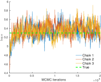
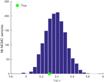
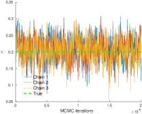
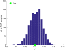
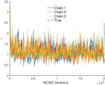
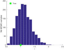
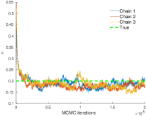
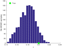
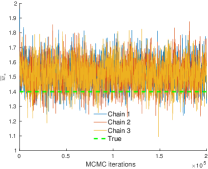
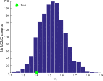
We first study the convergence of the MCMC algorithm on synthetic data simulated from the CCRM based graph model described in Section 2 where F𝐹F and ρ0subscript𝜌0\rho_{0} take the form (20) and (21). We generate an undirected graph with p=2𝑝2p=2 communities and parameters α=200𝛼200\alpha=200, σ=0.2𝜎0.2\sigma=0.2, τ=1𝜏1\tau=1, bk=b=1psubscript𝑏𝑘𝑏1𝑝b_{k}=b=\frac{1}{p}, ak=a=0.2subscript𝑎𝑘𝑎0.2a_{k}=a=0.2 and γk=γ=0subscript𝛾𝑘𝛾0\gamma_{k}=\gamma=0. The sampled graph has 112111211121 nodes and 609060906090 edges. For the inference, we consider that b𝑏b and γ𝛾\gamma are known and we assume a vague prior Gamma(0.01,0.01)Gamma0.010.01\mbox{Gamma}(0.01,0.01) on the unknown parameters α𝛼\alpha and ϕ=(1σ,τ,a)italic-ϕ1𝜎𝜏𝑎\phi=(1-\sigma,\tau,a). We run 333 parallel MCMC chains with different initial values. Each chain starts with 100001000010000 iterations using our model with only one community where the scores β𝛽\beta are fixed to 111, which is equivalent to the model of Caron and Fox (2017). We then run 200000200000200000 iterations using our model with p𝑝p communities. We use ε=103𝜀superscript103\varepsilon=10^{-3} as a truncation level for simulating w1:psubscript𝑤absent1:absent𝑝w_{\ast 1:p} and L=10𝐿10L=10 leapfrog steps for the HMC. The stepsizes of both the HMC and the random walk MH on (log(1σ),logτ,loga)1𝜎𝜏𝑎\left(\log(1-\sigma),\log\tau,\log a\right) are adapted during the first 500005000050000 iterations so as to target acceptance ratios of 0.650.650.65 and 0.230.230.23 respectively. The computations take around 111h101010 using Matlab on a standard desktop computer. Trace plots of the parameters logα𝛼\log\alpha, σ𝜎\sigma, τ𝜏\tau, a𝑎a and w¯=1pk=1pwksubscript¯𝑤1𝑝superscriptsubscript𝑘1𝑝subscript𝑤absent𝑘\overline{w}_{\ast}=\frac{1}{p}\sum_{k=1}^{p}w_{\ast k} and histograms based on the last 500005000050000 iterations are given in Figure 6. Posterior samples clearly converge around the sampled value. Aiming to study further the rate of convergence of our algorithm, we explore the impact of a lower threshold value ε𝜀\varepsilon and a higher number of iterations. Firstly, decreasing the threshold ε𝜀\varepsilon to a value 103much-less-thanabsentsuperscript103\ll 10^{-3} does not lead to any noticeable change in the MCMC histograms, suggesting that the target distribution of our approximate MCMC is very close to the posterior distribution of interest. Similarly, our approximate MCMC posterior obtained from running the algorithm for 106superscript10610^{6} iterations is very close to the one obtained from 200000200000200000 iterations.

Refer to caption
Refer to caption
(a) logα𝛼\log\alpha
Refer to caption
Refer to caption
(b) σ𝜎\sigma
Refer to caption
Refer to caption
(c) τ𝜏\tau
Refer to caption
Refer to caption
(d) a𝑎a
Refer to caption
Refer to caption
(e) w¯subscript¯𝑤\overline{w}_{\ast}
Figure 6: MCMC trace plots (left) and histograms (right) of parameters (a) logα𝛼\log\alpha, (b) σ𝜎\sigma, (c) τ𝜏\tau, (d) a𝑎a and (e) w¯subscript¯𝑤\overline{w}_{\ast} for a graph generated with parameters p=2𝑝2p=2, α=200𝛼200\alpha=200, σ=0.2𝜎0.2\sigma=0.2, τ=1𝜏1\tau=1, b=1p𝑏1𝑝b=\frac{1}{p}, a=0.2𝑎0.2a=0.2 and γ=0𝛾0\gamma=0.

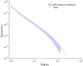
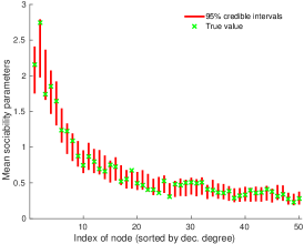
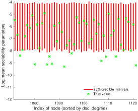
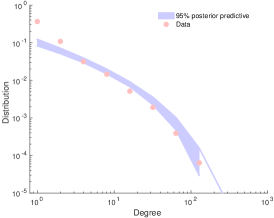
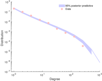
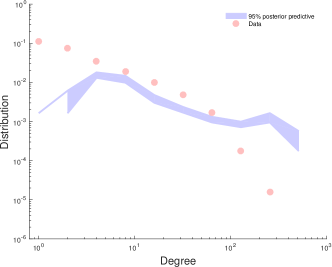
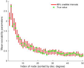
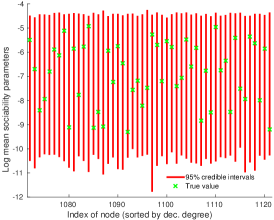
Our model is able to accurately recover the mean parameters of both low and high degree nodes and to provide reasonable credible intervals, as shown in Figure 7(a-b). By generating 500050005000 graphs from the posterior predictive we assess that our model fits the empirical power-law degree distribution of the sparse generated graph as shown in Figure 7(c). We demonstrate the interest of our nonparametric approach by comparing these results to the ones obtained with the parametric version of our model. To achieve this, we fix wk=0subscript𝑤absent𝑘0w_{\ast k}=0 and force the model to lie in the finite-activity domain by assuming σ(,0)𝜎0\sigma\in(-\infty,0{)} and using the prior distribution σGamma(0.01,0.01)similar-to𝜎Gamma0.010.01-\sigma\sim\mbox{Gamma}(0.01,0.01). Note that in this case, the model is equivalent to that of Zhou (2015). As shown in Figure 8(a-b), the parametric model is able to recover the mean parameters of nodes with high degrees, and credible intervals are similar to that obtained with the full model; however, it fails to provide reasonable credible intervals for nodes with low degree. In addition, as shown in Figure 8(c), the posterior predictive degree distribution does not fit the data, illustrating the unability of this parametric model to capture power-law behaviour.
Refer to caption
(a) 50 nodes with highest degrees
Refer to caption
(b) 50 nodes with lowest degrees
Refer to caption
(c) Degree distribution
Figure 7: 95% posterior credible intervals and true values of (a) the mean parameters w¯i=1pk=1pwiksubscript¯𝑤𝑖1𝑝superscriptsubscript𝑘1𝑝subscript𝑤𝑖𝑘\overline{w}_{i}=\frac{1}{p}\sum_{k=1}^{p}w_{ik} of the 50 nodes with highest degrees and (b) the log mean parameters logw¯isubscript¯𝑤𝑖\log\overline{w}_{i} of the 50 nodes with lowest degrees. (c) Empirical degree distribution and 95% posterior predictive credible interval. Results obtained for a graph generated with parameters p=2𝑝2p=2, α=200𝛼200\alpha=200, σ=0.2𝜎0.2\sigma=0.2, τ=1𝜏1\tau=1, b=1p𝑏1𝑝b=\frac{1}{p}, a=0.2𝑎0.2a=0.2 and γ=0𝛾0\gamma=0.
Refer to caption
(a) 50 nodes with highest degrees
Refer to caption
(b) 50 nodes with lowest degrees
Refer to caption
(c) Degree distribution
Figure 8: See Figure 7. Results obtained on the same generated graph by inferring a finite-activity model with wk=0subscript𝑤absent𝑘0w_{\ast k}=0 and σ0𝜎0\sigma\leq 0.

5.2 Real-world graphs

We now apply our methods to learn the latent communities of two real-world undirected simple graphs. The first network to be considered, the polblogs network (Adamic and Glance, 2005), is the network of the American political blogosphere in February 2005333http://www.cise.ufl.edu/research/sparse/matrices/Newman/polblogs. Two blogs are considered as connected if there is at least one hyperlink from one blog to the other. Additional information on the political leaning of each blog (left/right) is also available. The second network, named USairport, is the network of airports with at least one connection to a US airport in 2010444http://www.transtats.bts.gov/DL_SelectFields.asp?Table_ID=292.

Table 1: Size of the networks, number of communities and computational time.
Name Nb nodes Nb edges Nb communities p𝑝p Time
polblogs 122412241224 167151671516715 222 202020m
USairport 157415741574 172151721517215 444 111h

The sizes of the different networks are given in Table 1. We consider γk=0subscript𝛾𝑘0\gamma_{k}=0 is known and we assume a vague prior Gamma(0.01,0.01)Gamma0.010.01\mbox{Gamma}(0.01,0.01) on the unknown parameters α𝛼\alpha, 1σ1𝜎1-\sigma, τ𝜏\tau, aksubscript𝑎𝑘a_{k} and bksubscript𝑏𝑘b_{k}. We take p=2𝑝2p=2 communities for polblogs and p=4𝑝4p=4 communities for USairport. We run 333 parallel MCMC chains, each with 10000+20000010000200000$10000$+$200000$ iterations, using the same procedure as used for the simulated data; see Section 5.1. Computation times are reported in Table 1. The simulation of w1:psubscript𝑤absent1:absent𝑝w_{\ast 1:p} requires more computational time when σ0𝜎0\sigma\geq 0 (infinite-activity case). This explain the larger computation times for USairport compared to polblogs.

We interpret the communities based on the minimum Bayes risk point estimate where the cost function is a permutation-invariant absolute loss on the weights w=(wik)i=1,,Nα;k=1,,p𝑤subscriptsubscript𝑤𝑖𝑘formulae-sequence𝑖1subscript𝑁𝛼𝑘1𝑝w=(w_{ik})_{i=1,\ldots,N_{\alpha}{;}k=1,\ldots,p}. Let 𝒮psubscript𝒮𝑝\mathcal{S}_{p} be the set of permutations of {1,,p}1𝑝\{1,\ldots,p\} and consider the cost function

C(w,w)=minπ𝒮p[k=1pi=1Nα|wiπ(k)wik|+k=1p|wπ(k)wk|]𝐶𝑤superscript𝑤subscript𝜋subscript𝒮𝑝superscriptsubscript𝑘1𝑝superscriptsubscript𝑖1subscript𝑁𝛼subscript𝑤𝑖𝜋𝑘superscriptsubscript𝑤𝑖𝑘superscriptsubscript𝑘1𝑝subscript𝑤absent𝜋𝑘superscriptsubscript𝑤absent𝑘C\left(w,w^{\star}\right)=\min_{\pi\in\mathcal{S}_{p}}\left[\sum_{k=1}^{p}\sum_{i=1}^{N_{\alpha}}\left|w_{i\pi(k)}-w_{ik}^{\star}\right|+\sum_{k=1}^{p}\left|w_{\ast\pi(k)}-w_{\ast k}^{\star}\right|\right]

whose evaluation requires solving a combinatorial optimization problem in O(p3)𝑂superscript𝑝3O\left(p^{3}\right) using the Hungarian method. We therefore want to solve

w^=argminw𝔼[C(w,w)|Z]^𝑤superscript𝑤𝔼delimited-[]conditional𝐶𝑤superscript𝑤𝑍\widehat{w}=\underset{w^{\star}}{\arg\min}\,\mathbb{E}\left[C\left(w,w^{\star}\right)|Z\right]

where 𝔼[C(w,w)|Z]1Nt=1NC(w(t),w)similar-to-or-equals𝔼delimited-[]conditional𝐶𝑤superscript𝑤𝑍1𝑁superscriptsubscript𝑡1𝑁𝐶superscript𝑤𝑡superscript𝑤\mathbb{E}\left[C\left(w,w^{\star}\right)|Z\right]\simeq\frac{1}{N}\sum_{t=1}^{N}C\left(w^{(t)},w^{\star}\right) and (w(t))t=1,,Nsubscriptsuperscript𝑤𝑡𝑡1𝑁\left(w^{(t)}\right)_{t=1,\ldots,N} are from the MCMC output. For simplicity, we limit the search of w^^𝑤\widehat{w} to the set of MCMC samples giving

w^=argminw{w(1),,w(N)}1Nt=1NC(w(t),w).^𝑤superscript𝑤superscript𝑤1superscript𝑤𝑁1𝑁superscriptsubscript𝑡1𝑁𝐶superscript𝑤𝑡superscript𝑤\widehat{w}=\underset{w^{\star}\in\left\{w^{(1)},\ldots,w^{(N)}\right\}}{\arg\min}\frac{1}{N}\sum_{t=1}^{N}C\left(w^{(t)},w^{\star}\right).
Refer to caption
(a) polblogs
Refer to caption
(b) USairport
Figure 9: Adjacency matrices of the (a) polblogs and (b) USairport networks, reordered by associating each node to the community where it has the highest weight.
Table 2: Nodes with highest weight in each community for the polblogs network. Blog URLs are followed by known political leaning: (L) for left-wing and (R) for right-wing.
Community 1: “Liberal” Community 2: “Conservative”
dailykos.com (L)
atrios.blogspot.com (L)
talkingpointsmemo.com (L)
washingtonmonthly.com (L)
liberaloasis.com (L)
talkleft.com (L)
digbysblog.blogspot.com (L)
newleftblogs.blogspot.com (L)
politicalstrategy.org (L)
juancole.com (L) instapundit.com (R)
blogsforbush.com (R)
powerlineblog.com (R)
drudgereport.com (R)
littlegreenfootballs.com/weblog (R)
michellemalkin.com (R)
lashawnbarber.com (R)
wizbangblog.com (R)
hughhewitt.com (R)
truthlaidbear.com (R)

Table 3: Nodes with highest weights in each community for the USairport network.
Community 1: “Hub” Community 2: “East” Community 3: “West” Community 4: “Alaska”
Miami, FL
New York, NY
Newark, NJ
Los Angeles, CA
Atlanta, GA
Washington, DC
Chicago, IL
Boston, MA
Houston, TX
Orlando, FL Cleveland, OH
Detroit, MI
Nashville, TN
Chicago, IL
Knoxville, TN
Atlanta, GA
Louisville, KY
Indianapolis, IN
Memphis, TN
Charlotte, NC Denver, CO
Las Vegas, NV
Los Angeles, CA
Salt Lake City, UT
Seattle, WA
Burbank, CA
Phoenix, AZ
Oakland, CA
Portland, OR
Albuquerque, NM Anchorage, AK
Fairbanks, AK
Bethel, AK
St. Mary’s, AK
King Salmon, AK
McGrath, AK
Unalakleet, AK
Galena, AK
Aniak, AK
Kotzebue, AK
Refer to caption
Figure 10: Level of affiliation of each blog of the polblogs network to the communities identified as “Liberal” (top) and “Conservative” (bottom). The names of the blogs are grouped according to the left-right wing ground truth. Left-wing blogs are represented in blue on the left, right-wing blogs in red on the right.
Refer to caption
(a) polblogs
Refer to caption
(b) USairport
Figure 11: Relative values of the weights in each community for a subset of the nodes of the (a) polblogs and (b) USairport networks.

Table 5.2 reports the nodes with highest weights in each community for the polblogs network. Figure 10 also shows the weight associated to each of the two community alongside the true left/right class for each blog. The two learned communities, which can be interpreted as “Liberal” and “Conservative”, clearly recover the political leaning of the blogs. Figure 9 shows the adjacency matrices obtained by reordering the nodes by community membership, where each node is assigned to the community whose weight is maximum, clearly showing the block-structure of this network. The obtained clustering yields a 93.9593.9593.95% accuracy when compared to the ground truth classification. Figure 11(a) shows the relative community proportions for a subset of the blogs. dailykos.com and washingtonmonthly.com are clearly described as liberal while blogsforbush.com, instapundit.com and drudgereport.com are clearly conservative. Other more moderate blogs such as danieldrezner.com/blog and andrewsullivan.com have more balanced values in both communities. Figure 12(a) shows that the posterior predictive degree distribution provides a good fit to the data.

For USairport, the four learned communities can also be easily interpreted, as seen in Table 5.2. The first community, labeled “Hub”, represents highly connected airports with no preferred location, while the three others, labeled “East”, “West” and “Alaska”, are communities based on the location of the airport. In Figure 11(b), we can see that some airports have a strong level of affiliation in a single community: New York and Miami for “Hub”, Lansing for “East”, Seattle for “West” and Bethel and Anchorage for “Alaska”. Other airports have significant weights in different communities: Raleigh/Durham and Los Angeles are hubs with strong regional connections, Nashville and Minneapolis share a significant number of connections with both East and West of the USA. Anchorage has a significant “Hub” weight, while most airports in Alaska are disconnected from the rest of the world as can be seen in Figure 9(b). “Alaska” appears as a separate block while substantial overlaps are observed between the “Hub”, “East” and “West” communities. Figure 12(b) shows that the posterior predictive degree distribution also provides a good fit to the data.

5.3 Comparisons
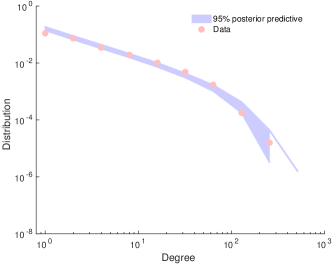
Refer to caption
(a) polblogs
Refer to caption
(b) USairport
Refer to caption
(c) polblogs
Refer to caption
(d) USairport
Refer to caption
(e) polblogs
Refer to caption
(f) USairport
Figure 12: Empirical degree distribution (red) and posterior predictive (blue) of the (left) polblogs and (right) USairport networks under our (top row) CCRM model, (middle row) MMSB and the (bottom row) MLFM.
Refer to caption
(a) polblogs
Refer to caption
(b) USairport
Refer to caption
(c) polblogs
Refer to caption
(d) USairport
Figure 13: Posterior predictive plots for the polblogs and USairport networks under the CCRM, MLFM and MMSB models. Top row: standard deviation of degree; bottom row: cluster coefficient

We compare the fit of our model to the mixed membership stochastic blockmodel (MMSB) of Airoldi et al. (2008) and the multiplicative latent factor model (MLFM) of Hoff (2009). The two models are briefly explained below.

Multiplicative latent factor model

Let XN×N𝑋superscript𝑁𝑁X\in\mathbb{R}^{N\times N} denote a (symmetric) random matrix of effects for a set of N𝑁N nodes. Under this model, X𝑋X is explained as the sum of systematic patterns and random noise. Y𝑌Y denotes the adjacency matrix. For 1i<jN1𝑖𝑗𝑁1\leq i<j\leq N

Xijsubscript𝑋𝑖𝑗\displaystyle X_{ij} =ξ0+ζi+ζj+Mij+Eijabsentsubscript𝜉0subscript𝜁𝑖subscript𝜁𝑗subscript𝑀𝑖𝑗subscript𝐸𝑖𝑗\displaystyle=\xi_{0}+\zeta_{i}+\zeta_{j}+M_{ij}+E_{ij}
Yijsubscript𝑌𝑖𝑗\displaystyle Y_{ij} =𝟙Xij>0absentsubscript1subscript𝑋𝑖𝑗0\displaystyle=\mathds{1}_{X_{ij}>0}

where ξ0subscript𝜉0\xi_{0}\in\mathbb{R} is the intercept, ζisubscript𝜁𝑖\zeta_{i}\in\mathbb{R} is the additive node effect, MN×N𝑀superscript𝑁𝑁M\in\mathbb{R}^{N\times N} is the matrix of multiplicative effects. The square symmetric matrix M𝑀M has a latent decomposition of the form M=UΛUT,𝑀𝑈Λsuperscript𝑈𝑇M=U\Lambda U^{T}, where UN×p𝑈superscript𝑁𝑝U\in\mathbb{R}^{N\times p} and Λp×pΛsuperscript𝑝𝑝\Lambda\in\mathbb{R}^{p\times p} is a diagonal matrix. EN×N𝐸superscript𝑁𝑁E\in\mathbb{R}^{N\times N} is the matrix of standard normal noise; Eijiid𝒩(0,1)subscript𝐸𝑖𝑗iidsimilar-to𝒩01E_{ij}\overset{\text{iid}}{\sim}\mathcal{N}(0,1). Denoting by uisubscript𝑢𝑖u_{i} the ithsuperscript𝑖thi^{\text{th}} row of U𝑈U we have Mij=uiTΛujsubscript𝑀𝑖𝑗subscriptsuperscript𝑢𝑇𝑖Λsubscript𝑢𝑗M_{ij}=u^{T}_{i}\Lambda u_{j}. We use the priors implemented in the package amen. For the additive effect ζisubscript𝜁𝑖\zeta_{i} it is assumed that ζii.i.d.𝒩(0,σζ2)subscript𝜁𝑖i.i.d.similar-to𝒩0superscriptsubscript𝜎𝜁2\,\zeta_{i}\overset{\text{i.i.d.}}{\sim}\mathcal{N}(0,\sigma_{\zeta}^{2}), with 1/σζ2Gamma(12,12)similar-to1superscriptsubscript𝜎𝜁2Gamma12121/\sigma_{\zeta}^{2}\sim\text{Gamma}\left(\frac{1}{2},\frac{1}{2}\right). For the multiplicative effects it is assumed that uijind𝒩(0,σj2)subscript𝑢𝑖𝑗indsimilar-to𝒩0superscriptsubscript𝜎𝑗2\,u_{ij}\overset{\text{ind}}{\sim}\mathcal{N}(0,\sigma_{j}^{2}) with 1/σj2Gamma(2,1)similar-to1superscriptsubscript𝜎𝑗2Gamma211/\sigma_{j}^{2}\sim\text{Gamma}(2,1). For ξ0subscript𝜉0\xi_{0} we use an improper prior p(ξ0)1/ξ0proportional-to𝑝subscript𝜉01subscript𝜉0p(\xi_{0})\propto 1/\xi_{0}.

Mixed membership stochastic blockmodel

Let N𝑁N be the number of nodes in the network and Y𝑌Y the adjacency matrix. For each node i=1,,N𝑖1𝑁i=1,\ldots,N, let π_i∼Dirichlet(ς,…,ς) be a p𝑝p dimensional mixed membership probability vector for node i𝑖i, with ς>0𝜍0\varsigma>0. For each pair of nodes i<j𝑖𝑗i<j, let

cij|πiconditionalsubscript𝑐𝑖𝑗subscript𝜋𝑖\displaystyle c_{ij}|\pi_{i} πisimilar-toabsentsubscript𝜋𝑖\displaystyle\sim\pi_{i}
cji|πjconditionalsubscript𝑐𝑗𝑖subscript𝜋𝑗\displaystyle c_{ji}|\pi_{j} πjsimilar-toabsentsubscript𝜋𝑗\displaystyle\sim\pi_{j}
Yij|cij,cji,Bconditionalsubscript𝑌𝑖𝑗subscript𝑐𝑖𝑗subscript𝑐𝑗𝑖𝐵\displaystyle Y_{ij}|c_{ij},c_{ji},B Bernoulli{(1ρ)Bcijcji}similar-toabsentBernoulli1𝜌subscript𝐵subscript𝑐𝑖𝑗subscript𝑐𝑗𝑖\displaystyle\sim\text{Bernoulli}\left\{\left(1-\rho\right)B_{c_{ij}c_{ji}}\right\}

where cij{1,,p}subscript𝑐𝑖𝑗1𝑝c_{ij}\in\{1,\ldots,p\} is the emission indicator variable, ρ𝜌\rho is a parameter that controls the proportion of zeros that should not be explained by the blockmodel and B𝐵B is the p×p𝑝𝑝p\times p matrix that contains the Bernoulli rates of the link probabilities between different communities, i.e. Bk,lsubscript𝐵𝑘𝑙B_{k,l} is the probability of a connection between a member of group k𝑘k and one of group l𝑙l. We assume ςGamma(1,1)similar-to𝜍Gamma11\varsigma\sim\text{Gamma}(1,1), ρBeta(1/2,1/2)similar-to𝜌Beta1212\rho\sim\text{Beta}(1/2,1/2) and Bk,Beta(1,1)similar-tosubscript𝐵𝑘Beta11B_{k,\ell}\sim\text{Beta}(1,1).

For each model, we run three MCMC chains for posterior inference, using the amen R package (Hoff et al., 2017) for MLFM. Under MMSB, we use 200000200000200000 MCMC iterations, of which 100000100000100000 discarded as burn in. Under MLFM, which required more iterations to converge, we ran 1M1𝑀1M iterations, of which 500000500000500000 discarded as burn-in. In both cases we thinned the output to obtain 500 samples approximately distributed from the posterior distribution.

Posterior predictive checks.

In order to evaluate the goodness of fit of each model, we look at some statistics of a replicated network for a new set of nodes, sampled under the posterior predictive. Let Ysuperscript𝑌Y^{*} be a N𝑁N by N𝑁N adjacency matrix corresponding to the edges of a set of N𝑁N new nodes, sampled from

Pr(Y|Y)={Pr(Y|ξ0,Λ)Pr(dξ0,dΛ|Y) for MLFMPr(Y|ς,ρ,B)Pr(dς,dρ,dB|Y) for MMSBPrconditionalsuperscript𝑌𝑌casesPrconditionalsuperscript𝑌subscript𝜉0ΛPr𝑑subscript𝜉0conditional𝑑Λ𝑌 for MLFMPrconditionalsuperscript𝑌𝜍𝜌𝐵Pr𝑑𝜍𝑑𝜌conditional𝑑𝐵𝑌 for MMSB\displaystyle\Pr(Y^{*}|Y)=\left\{\begin{array}[]{ll}\int\Pr(Y^{*}|\xi_{0},\Lambda)\Pr(d\xi_{0},d\Lambda|Y)&\text{ for MLFM}\\ \int\Pr(Y^{*}|\varsigma,\rho,B)\Pr(d\varsigma,d\rho,dB|Y)&\text{ for MMSB}\end{array}\right.

Note that the posterior predictive setting is different from that of Hoff (2009), which replicates a network for the same set of nodes and therefore conditions on the parameters ui,ζisubscript𝑢𝑖subscript𝜁𝑖u_{i},\zeta_{i}. We generate 500 samples from the posterior predictive under each model. We are interested in some standard summary statistics: the degree distribution, standard deviation of the degrees and cluster coefficient. Posterior degree distributions under each model for polblogs and USairport are presented in Figure 12 and posterior predictive distributions of the standard deviation of the degree and clustering coefficient in Figure 13.

Overall, the MMSB did not perform well on the two datasets considered. While being a very flexible model, applied successfully to a wide range of real-world networks, the MMSB doesn’t explicitly capture degree heterogeneity; the latent communities recovered (not shown) do not correspond to those recovered by CCRM or MLFM: it tends to cluster nodes according to their degree, explaining the shape of the posterior degree predictive in Figure 12(c-d) . Such limitations, due to the lack of degree correction, have been acknowledged by previous authors (Karrer and Newman, 2011; Gopalan et al., 2013). Note that degree-corrected MMSB have been proposed by Gopalan et al. (2013), similar to the general class of models discussed in (Hoff, 2009).

MLFM on the other hand incorporates degree heterogeneity and thus gives better fit on the degree predictive distribution. It also gives similar results than CCRM and recovers similar latent communities. However, by construction this model cannot capture sparsity or heavy tailed degree distributions. It underestimates the proportion of nodes with degree one as shown in Figure 12 (top row). While our CCRM model over-estimates the proportion of nodes of degree one, it tends to give a better fit to the empirical degree distribution overall. Finally, in Figure 13, we report the goodness of fit statistics used in the analyses of Hoff (2009). The first one is the standard deviation of the degree shown in the middle row, on which MMSB performs poorly, whereas CCRM and MLFM have similar results, marginally close to the empirical value. The bottom row reports the cluster coefficient, also known as triadic dependence. In this case, CCRM gives a better fit on the sparse USairport dataset while MFLM gives a better result than CCRM on the dense polblogs dataset.

Acknowledgments

The authors thank George Deligiannidis for pointing out the article of Asmussen and Rosiński (2001). FC acknowledges the support of the European Commission under the Marie Curie Intra-European Fellowship Programme. Part of this work has been supported by the BNPSI ANR project no ANR-13-BS-03-0006-01.

Appendix A Background on completely random measures

A.1 Completely random measures

Completely random measures (CRM) were introduced by Kingman (1967, 1993) and are now standard tools for constructing flexible Bayesian nonparametric (BNP) models; see for example the surveys of Lijoi and Prünster (2010) or Daley and Vere-Jones (2008b, Section 10.1).

A CRM W𝑊W on +subscript\mathbb{R}_{+} is a random measure such that, for any collection of disjoint measurable subsets A1,,Ansubscript𝐴1subscript𝐴𝑛A_{1},\ldots,A_{n} of +subscript\mathbb{R}_{+}, W(A1),,W(An)𝑊subscript𝐴1𝑊subscript𝐴𝑛W(A_{1}),\ldots,W(A_{n}) are independent. A CRM can be decomposed into a sum of three independent parts: a non-random measure, a countable collection of atoms with random masses at fixed locations, and a countable collection of atoms with random masses and random locations. Here, we will only consider CRMs with random masses and random locations, which take the form

W=i=1wiδθi𝑊superscriptsubscript𝑖1subscript𝑤𝑖subscript𝛿subscript𝜃𝑖W=\sum_{i=1}^{\infty}w_{i}\delta_{\theta_{i}} (49)

where the wi+subscript𝑤𝑖subscriptw_{i}\in\mathbb{R}_{+} are the masses and θi+subscript𝜃𝑖subscript\theta_{i}\in\mathbb{R}_{+} are the locations. The law of W𝑊W can actually be characterized by a Poisson point process N={(wi,θi)i=1,2,}𝑁subscriptsubscript𝑤𝑖subscript𝜃𝑖𝑖12N=\{(w_{i},\theta_{i})_{i=1,2,\ldots}\} on +2superscriptsubscript2\mathbb{R}_{+}^{2} with mean measure ν(dw,dθ)𝜈𝑑𝑤𝑑𝜃\nu(dw,d\theta). We focus here on the case where the CRM is homogeneous with independent increments. This implies that the location θisubscript𝜃𝑖\theta_{i} are independent of the weights wisubscript𝑤𝑖w_{i} and the mean measure decomposes as ν(dw,dθ)=ρ(dw)λ(dθ)𝜈𝑑𝑤𝑑𝜃𝜌𝑑𝑤𝜆𝑑𝜃\nu(dw,d\theta)=\rho(dw)\lambda(d\theta) where λ𝜆\lambda is the Lebesgue measure and ρ𝜌\rho is a measure on +subscript\mathbb{R}_{+} such that

0(1ew)ρ(dw)<.superscriptsubscript01superscript𝑒𝑤𝜌𝑑𝑤\int_{0}^{\infty}(1-e^{-w})\rho(dw)<\infty. (50)

We write WCRM(ρ,λ)similar-to𝑊CRM𝜌𝜆W\sim\operatorname{CRM}(\rho,\lambda). Note that W([0,T])<𝑊0𝑇W([0,T])<\infty a.s. for any real T𝑇T while W(+)=𝑊subscriptW(\mathbb{R}_{+})=\infty a.s. if ρ𝜌\rho is not degenerate at 00. If

0ρ(dw)=superscriptsubscript0𝜌𝑑𝑤\int_{0}^{\infty}\rho(dw)=\infty (51)

then there will be a.s. an infinite number of jumps in any interval [0,T]0𝑇[0,T] and we refer to the CRM as infinite-activity. Otherwise, it is called finite activity. Let ρ¯¯𝜌\overline{\rho} be the tail Lévy intensity defined as

ρ¯(x)=xρ(dw)¯𝜌𝑥superscriptsubscript𝑥𝜌𝑑𝑤\overline{\rho}(x)=\int_{x}^{\infty}\rho(dw) (52)

for x>0𝑥0x>0. This function corresponds to the expected number of points (wi,θi)subscript𝑤𝑖subscript𝜃𝑖(w_{i},\theta_{i}) such that wi>xsubscript𝑤𝑖𝑥w_{i}>x and θi[0,1]subscript𝜃𝑖01\theta_{i}\in[0,1], and its asymptotic properties play an important role in the characterization of the graph properties.

A.2 Vectors of CRMs

Multivariate extensions of CRMs have been proposed recently by various authors (Epifani and Lijoi, 2010; Leisen and Lijoi, 2011; Leisen et al., 2013; Griffin et al., 2013; Lijoi et al., 2014). These models are closely related to Lévy copulas (Tankov, 2003; Cont and Tankov, 2003; Kallsen and Tankov, 2006) and multivariate subordinators on cones (Barndorff-Nielsen et al., 2001; Skorohod, 1991). A vector of CRMs (W1,,Wp)subscript𝑊1subscript𝑊𝑝(W_{1},\ldots,W_{p}) on +subscript\mathbb{R}_{+} is a collection of random measures Wksubscript𝑊𝑘W_{k}, k=1,,p𝑘1𝑝k=1,\ldots,p, such that, for any collection of disjoint measurable subsets A1,,Ansubscript𝐴1subscript𝐴𝑛A_{1},\ldots,A_{n} of +subscript\mathbb{R}_{+}, the vectors (W1(A1),,Wp(A1))subscript𝑊1subscript𝐴1subscript𝑊𝑝subscript𝐴1(W_{1}(A_{1}),\ldots,W_{p}(A_{1})), (W1(A2),,Wp(A2))subscript𝑊1subscript𝐴2subscript𝑊𝑝subscript𝐴2(W_{1}(A_{2}),\ldots,W_{p}(A_{2})),…,(W1(An),,Wp(An))subscript𝑊1subscript𝐴𝑛subscript𝑊𝑝subscript𝐴𝑛(W_{1}(A_{n}),\ldots,W_{p}(A_{n})) are mutually independent. We only consider here vectors of CRMs with both random weights and locations. In this case, the measures Wksubscript𝑊𝑘W_{k}, k=1,,p𝑘1𝑝k=1,\ldots,p, are a.s. discrete and take the form

Wk=i=1wikδθi.subscript𝑊𝑘superscriptsubscript𝑖1subscript𝑤𝑖𝑘subscript𝛿subscript𝜃𝑖W_{k}=\sum_{i=1}^{\infty}w_{ik}\delta_{\theta_{i}}. (53)

The law of the vector of CRMs can be characterized by a Poisson point process on +p+1subscriptsuperscript𝑝1\mathbb{R}^{p+1}_{+} with mean measure ν(dw1,,dwp,dθ)𝜈𝑑subscript𝑤1𝑑subscript𝑤𝑝𝑑𝜃\nu(dw_{1},\ldots,dw_{p},d\theta). We focus again on homogeneous vectors of CRMs with independent increments where the mean measure can be written as

ν(dw1,,dwp,dθ)=ρ(dw1,,dwp)λ(dθ).𝜈𝑑subscript𝑤1𝑑subscript𝑤𝑝𝑑𝜃𝜌𝑑subscript𝑤1𝑑subscript𝑤𝑝𝜆𝑑𝜃\nu(dw_{1},\ldots,dw_{p},d\theta)=\rho(dw_{1},\ldots,dw_{p})\lambda(d\theta). (54)

where ρ𝜌\rho is a measure on +psubscriptsuperscript𝑝\mathbb{R}^{p}_{+}, concentrated on +p\{𝟎}\subscriptsuperscript𝑝0\mathbb{R}^{p}_{+}\backslash\{\mathbf{0}\}, which satisfies

+pmin(1,k=1pwk)ρ(dw1,,dwp)<.subscriptsuperscriptsubscript𝑝1superscriptsubscript𝑘1𝑝subscript𝑤𝑘𝜌𝑑subscript𝑤1𝑑subscript𝑤𝑝\int_{\mathbb{R}_{+}^{p}}\min\left(1,{\sum_{k=1}^{p}w_{k}}\right)\rho(dw_{1},\ldots,dw_{p})<\infty. (55)

We use the same notation as for (scalar) CRMs and write simply (W1,,Wp)CRM(ρ,λ)similar-tosubscript𝑊1subscript𝑊𝑝CRM𝜌𝜆(W_{1},\ldots,W_{p})\sim\text{CRM}(\rho,\lambda). A key quantity is the multivariate Laplace exponent defined by

ψ(t1,,tp)𝜓subscript𝑡1subscript𝑡𝑝\displaystyle\psi(t_{1},\ldots,t_{p}) :=log𝔼[ek=1ptkWk([0,1])]assignabsent𝔼delimited-[]superscript𝑒superscriptsubscript𝑘1𝑝subscript𝑡𝑘subscript𝑊𝑘01\displaystyle:=-\log\mathbb{E}\left[e^{-\sum_{k=1}^{p}t_{k}W_{k}([0,1])}\right] (56)
=+p(1ek=1ptkwk)ρ(dw1,,dwp)absentsubscriptsubscriptsuperscript𝑝1superscript𝑒superscriptsubscript𝑘1𝑝subscript𝑡𝑘subscript𝑤𝑘𝜌𝑑subscript𝑤1𝑑subscript𝑤𝑝\displaystyle=\int_{{\mathbb{R}^{p}_{+}}}\left(1-e^{-\sum_{k=1}^{p}t_{k}w_{k}}\right)\rho(dw_{1},\ldots,dw_{p}) (57)

Note that this quantity involves a p𝑝p-dimensional integral which may not be analytically computable, and may be expensive to evaluate numerically. As for CRMs, if

+pρ(dw1,,dwp)=subscriptsubscriptsuperscript𝑝𝜌𝑑subscript𝑤1𝑑subscript𝑤𝑝\int_{\mathbb{R}^{p}_{+}}\rho(dw_{1},\ldots,dw_{p})=\infty (58)

then there will be an infinite number of θi[0,T]subscript𝜃𝑖0𝑇\theta_{i}\in[0,T] for which kwik>0subscript𝑘subscript𝑤𝑖𝑘0\sum_{k}w_{ik}>0 and the vector of CRMs is called infinite-activity. Otherwise, it is called finite-activity. Note that some (but not all) CRMs may still be marginally finite-activity.

Appendix B Proof of Propositions 4 and 5

The proof of (Caron and Fox, 2017, Appendix C) can be directly adapted to the multivariate generalization presented in this paper. We only provide a sketch of the proof. First, as Z𝑍Z is a jointly exchangeable point process verifying (23) and under the moment condition (26), it follows from the law of large numbers that

Nα(e)=Θ(α2) a.s. as α.superscriptsubscript𝑁𝛼𝑒Θsuperscript𝛼2 a.s. as 𝛼N_{\alpha}^{(e)}=\Theta(\alpha^{2})\text{ a.s. as }\alpha\rightarrow\infty.

Finite-activity case.

If the vector of CRMs is finite-activity, the jump locations arise from an homogeneous Poisson process with finite rate, and Nα=Θ(α)subscript𝑁𝛼Θ𝛼N_{\alpha}=\Theta(\alpha) a.s. It follows that

Nα(e)=Θ(Nα2) a.s. as α.superscriptsubscript𝑁𝛼𝑒Θsubscriptsuperscript𝑁2𝛼 a.s. as 𝛼N_{\alpha}^{(e)}=\Theta(N^{2}_{\alpha})\text{ a.s. as }\alpha\rightarrow\infty.

Infinite-activity case.

Consider now the infinite-activity case. Following Caron and Fox (2017), one can lower bound the node counting process Nαsubscript𝑁𝛼N_{\alpha} by a counting process N~αsubscript~𝑁𝛼\widetilde{N}_{\alpha} which is conditionally Poisson, and the same proof applies. For infinite-activity CCRM, we use the fact that ψ(W1([0,α]),,Wp([0,α]))𝜓subscript𝑊10𝛼subscript𝑊𝑝0𝛼\psi(W_{1}([0,\alpha]),\ldots,W_{p}([0,\alpha]))\rightarrow\infty a.s., it follows that Nα=Ω(α)subscript𝑁𝛼Ω𝛼N_{\alpha}=\Omega(\alpha) a.s., and therefore

Nα(e)=o(Nα2) a.s. as α.superscriptsubscript𝑁𝛼𝑒𝑜subscriptsuperscript𝑁2𝛼 a.s. as 𝛼N_{\alpha}^{(e)}=o(N^{2}_{\alpha})\text{ a.s. as }\alpha\rightarrow\infty.

Finally, for compound CRMs with regularly varying ρ0subscript𝜌0\rho_{0} with exponent σ𝜎\sigma and slowly varying function such that limt(t)>0subscript𝑡𝑡0\lim_{t\rightarrow\infty}\ell(t)>0, Proposition G.9 in Appendix G implies that Nα=ω(α1+σ)subscript𝑁𝛼𝜔superscript𝛼1𝜎N_{\alpha}=\omega(\alpha^{1+\sigma}) a.s. and

Nα(e)=O(Nα2/(1+σ)) a.s. as α.superscriptsubscript𝑁𝛼𝑒𝑂superscriptsubscript𝑁𝛼21𝜎 a.s. as 𝛼N_{\alpha}^{(e)}=O(N_{\alpha}^{2/(1+\sigma)})\text{ a.s. as }\alpha\rightarrow\infty.

Appendix C Proof of Theorem 3

Let Dα=k=1pDkα([0,α])subscriptsuperscript𝐷𝛼superscriptsubscript𝑘1𝑝subscript𝐷𝑘𝛼0𝛼D^{*}_{\alpha}=\sum_{k=1}^{p}D_{k\alpha}([0,\alpha]) be the number of edges in the directed graph of size α𝛼\alpha, Wk,α=Wk([0,α])superscriptsubscript𝑊𝑘𝛼subscript𝑊𝑘0𝛼W_{k,\alpha}^{*}=W_{k}([0,\alpha]) and Wα=(W1,α,,Wp,α)Tsuperscriptsubscript𝑊𝛼superscriptsuperscriptsubscript𝑊1𝛼superscriptsubscript𝑊𝑝𝛼𝑇W_{\alpha}^{*}=(W_{1,\alpha}^{*},\ldots,W_{p,\alpha}^{*})^{T}. Using Campbell’s theorem,

𝔼[Dα]=𝔼[𝔼[Dα|Wα]]=𝔼[(Wα)TWα]=𝔼[Wα]T𝔼[Wα]+tr(cov(Wα))=α2μTμ+αtr(Σ)𝔼delimited-[]subscriptsuperscript𝐷𝛼𝔼delimited-[]𝔼delimited-[]conditionalsubscriptsuperscript𝐷𝛼subscriptsuperscript𝑊𝛼𝔼delimited-[]superscriptsubscriptsuperscript𝑊𝛼𝑇subscriptsuperscript𝑊𝛼𝔼superscriptdelimited-[]subscriptsuperscript𝑊𝛼𝑇𝔼delimited-[]subscriptsuperscript𝑊𝛼trcovsubscriptsuperscript𝑊𝛼superscript𝛼2superscript𝜇𝑇𝜇𝛼trΣ\begin{split}\mathbb{E}\left[D^{*}_{\alpha}\right]&=\mathbb{E}\left[\mathbb{E}\left[D^{*}_{\alpha}|W^{*}_{\alpha}\right]\right]=\mathbb{E}\left[(W^{*}_{\alpha})^{T}W^{*}_{\alpha}\right]\\ &=\mathbb{E}\left[W^{*}_{\alpha}\right]^{T}\mathbb{E}\left[W^{*}_{\alpha}\right]+\text{tr}(\text{cov}\left(W^{*}_{\alpha}\right))\\ &=\alpha^{2}\mu^{T}\mu+\alpha\text{tr}(\Sigma)\end{split} (59)

where we define μ= ∫_R^p_+ w ρ(dw_1,…,dw_p),    Σ= ∫_R^p_+ w w^T ρ(dw_1,…,dw_p).

Let wi=(wi1,,wip)subscript𝑤𝑖subscript𝑤𝑖1subscript𝑤𝑖𝑝w_{i}=(w_{i1},\ldots,w_{ip}). We have, using the extended Slivnyak-Mecke theorem (Møller and Waagepetersen, 2003, Theorem 3.3)

𝔼[Nα(e)]=𝔼[𝔼[Nα(e)|W1,,Wp]]=𝔼[i𝟙θiα[(1ewiTwi)+12ji𝟙θjα(1e2wiTwj)]]=α+p(1ewTw)ρ(dw1,,dwp)+α22+pψ(2w1,,2wp)ρ(dw1,,dwp).𝔼delimited-[]superscriptsubscript𝑁𝛼𝑒𝔼delimited-[]𝔼delimited-[]conditionalsubscriptsuperscript𝑁𝑒𝛼subscript𝑊1subscript𝑊𝑝𝔼delimited-[]subscript𝑖subscript1subscript𝜃𝑖𝛼delimited-[]1superscript𝑒superscriptsubscript𝑤𝑖𝑇subscript𝑤𝑖12subscript𝑗𝑖subscript1subscript𝜃𝑗𝛼1superscript𝑒2superscriptsubscript𝑤𝑖𝑇subscript𝑤𝑗𝛼subscriptsubscriptsuperscript𝑝1superscript𝑒superscript𝑤𝑇𝑤𝜌𝑑subscript𝑤1𝑑subscript𝑤𝑝superscript𝛼22subscriptsubscriptsuperscript𝑝𝜓2subscript𝑤12subscript𝑤𝑝𝜌𝑑subscript𝑤1𝑑subscript𝑤𝑝\begin{split}\mathbb{E}[N_{\alpha}^{(e)}]&=\mathbb{E}\left[\mathbb{E}[N^{(e)}_{\alpha}|W_{1},\ldots,W_{p}]\right]\\ &=\mathbb{E}\left[\sum_{i}\mathds{1}_{\theta_{i}\leq\alpha}\left[\left(1-e^{-w_{i}^{T}w_{i}}\right)+\frac{1}{2}\sum_{j\neq i}\mathds{1}_{\theta_{j}\leq\alpha}\left(1-e^{-2w_{i}^{T}w_{j}}\right)\right]\right]\\ &=\alpha\int_{\mathbb{R}^{p}_{+}}\left(1-e^{-w^{T}w}\right)\rho(dw_{1},\ldots,dw_{p})+\frac{\alpha^{2}}{2}\int_{\mathbb{R}^{p}_{+}}\psi(2w_{1},\ldots,2w_{p})\rho(dw_{1},\ldots,dw_{p}).\end{split} (60)

Using the extended Slivnyak-Mecke theorem then Campbell’s theorem,

𝔼[Nα]=𝔼[𝔼[Nα|W1,,Wp]]=𝔼[i(1e2wiT(jiwj1θjα)wiTwi)𝟙θiα]=α+p𝔼(1e2wT(jwj𝟙θjα)wTw)ρ(dw1,,dwp)=α+p(1ewTwαψ(2w1,,2wp))ρ(dw1,,dwp)𝔼delimited-[]subscript𝑁𝛼𝔼delimited-[]𝔼delimited-[]conditionalsubscript𝑁𝛼subscript𝑊1subscript𝑊𝑝𝔼delimited-[]subscript𝑖1superscript𝑒2superscriptsubscript𝑤𝑖𝑇subscript𝑗𝑖subscript𝑤𝑗subscript1subscript𝜃𝑗𝛼superscriptsubscript𝑤𝑖𝑇subscript𝑤𝑖subscript1subscript𝜃𝑖𝛼𝛼subscriptsuperscriptsubscript𝑝𝔼1superscript𝑒2superscript𝑤𝑇subscript𝑗subscript𝑤𝑗subscript1subscript𝜃𝑗𝛼superscript𝑤𝑇𝑤𝜌𝑑subscript𝑤1𝑑subscript𝑤𝑝𝛼subscriptsuperscriptsubscript𝑝1superscript𝑒superscript𝑤𝑇𝑤𝛼𝜓2subscript𝑤12subscript𝑤𝑝𝜌𝑑subscript𝑤1𝑑subscript𝑤𝑝\begin{split}\mathbb{E}[N_{\alpha}]&=\mathbb{E}\left[\mathbb{E}\left[N_{\alpha}|W_{1},\dots,W_{p}\right]\right]\\ &=\mathbb{E}\left[\sum_{i}\left(1-e^{-2w_{i}^{T}(\sum_{j\neq i}w_{j}1_{\theta_{j}\leq\alpha})-w_{i}^{T}w_{i}}\right)\mathds{1}_{\theta_{i}\leq\alpha}\right]\\ &=\alpha\int_{\mathbb{R}_{+}^{p}}\mathbb{E}\left(1-e^{-2w^{T}(\sum_{j}w_{j}\mathds{1}_{\theta_{j}\leq\alpha})-w^{T}w}\right)\rho(dw_{1},\ldots,dw_{p})\\ &=\alpha\int_{\mathbb{R}_{+}^{p}}\left(1-e^{-w^{T}w-\alpha\psi(2w_{1},\ldots,2w_{p})}\right)\rho(dw_{1},\ldots,dw_{p})\end{split} (61)

By monotone convergence, we have, as α𝛼\alpha tends to infinity, E[N_α]∼α∫_R_+^p ρ(dw_1,…,w_p) if the CRM is finite-activity and 𝔼[Nα]=ω(α)𝔼delimited-[]subscript𝑁𝛼𝜔𝛼\mathbb{E}[N_{\alpha}]=\omega(\alpha) otherwise.

Appendix D Simulation from a tilted truncated generalized gamma process

We want to sample points from a Poisson process with truncated mean measure

ρε(dw)=h(w)w1σeτw𝟙w>εdwsuperscript𝜌𝜀𝑑𝑤𝑤superscript𝑤1𝜎superscript𝑒𝜏𝑤subscript1𝑤𝜀𝑑𝑤\rho^{\varepsilon}(dw)=h(w)w^{-1-\sigma}e^{-\tau w}{\mathds{1}}_{w>\varepsilon}dw (62)

where hh is a monotone decreasing and bounded function, and (τ,σ)𝜏𝜎(\tau,\sigma) verify either τ0𝜏0\tau\geq 0 and σ(0,1)𝜎01\sigma\in(0,1), or τ>0𝜏0\tau>0 and σ(1,0]𝜎10\sigma\in(-1,0]. We will resort to adaptive thinning (Lewis and Shedler, 1979; Ogata, 1981; Favaro and Teh, 2013).

For τ>0𝜏0\tau>0, consider the family of adaptive bounds

gt(s)=h(t)t1σexp(τs)subscript𝑔𝑡𝑠𝑡superscript𝑡1𝜎𝜏𝑠g_{t}(s)=h(t)t^{-1-\sigma}\exp(-\tau s)

with gt(s)>ρ(s)subscript𝑔𝑡𝑠𝜌𝑠g_{t}(s)>\rho(s) for s>t𝑠𝑡s>t. We have,

Gt(s)subscript𝐺𝑡𝑠\displaystyle G_{t}(s) =tsgt(s)𝑑sabsentsuperscriptsubscript𝑡𝑠subscript𝑔𝑡superscript𝑠differential-dsuperscript𝑠\displaystyle=\int_{t}^{s}g_{t}(s^{\prime})ds^{\prime}
=h(t)τt1σ(exp(τt)exp(τs))absent𝑡𝜏superscript𝑡1𝜎𝜏𝑡𝜏𝑠\displaystyle=\frac{h(t)}{\tau}t^{-1-\sigma}(\exp(-\tau t)-\exp(-\tau s))

and

Gt1(r)superscriptsubscript𝐺𝑡1𝑟\displaystyle G_{t}^{-1}(r) =1τlog(exp(τt)rτt1σh(t)).absent1𝜏𝜏𝑡𝑟𝜏superscript𝑡1𝜎𝑡\displaystyle=-\frac{1}{\tau}\log\left(\exp(-\tau t)-\frac{r\tau}{t^{-1-\sigma}h(t)}\right).

For τ=0𝜏0\tau=0, we consider bounds

gt(s)=h(t)s1σsubscript𝑔𝑡𝑠𝑡superscript𝑠1𝜎g_{t}(s)=h(t)s^{-1-\sigma}

and we obtain

Gt(s)subscript𝐺𝑡𝑠\displaystyle G_{t}(s) =h(t)σ(tσsσ)absent𝑡𝜎superscript𝑡𝜎superscript𝑠𝜎\displaystyle=\frac{h(t)}{\sigma}(t^{-\sigma}-s^{-\sigma})
Gt1(r)superscriptsubscript𝐺𝑡1𝑟\displaystyle G_{t}^{-1}(r) =[tσrσh(t)]1/σ.absentsuperscriptdelimited-[]superscript𝑡𝜎𝑟𝜎𝑡1𝜎\displaystyle=\left[t^{-\sigma}-\frac{r\sigma}{h(t)}\right]^{-1/\sigma}.

The adaptive thinning sampling scheme is as follows:

  1. 1.

    Set N=,t=εformulae-sequence𝑁𝑡𝜀N=\emptyset,t=\varepsilon

  2. 2.

    iterate until termination

    1. (a)

      Draw rExp(1)similar-to𝑟Exp1r\sim\text{Exp}(1)

    2. (b)

      If r>Gt()𝑟subscript𝐺𝑡r>G_{t}(\infty), terminate; else set t=Gt1(r);superscript𝑡superscriptsubscript𝐺𝑡1𝑟t^{\prime}=G_{t}^{-1}(r);

    3. (c)

      with probability ρε(t)/gt(t)superscript𝜌𝜀superscript𝑡subscript𝑔𝑡superscript𝑡\rho^{\varepsilon}(t^{\prime})/g_{t}(t^{\prime}) accept sample tsuperscript𝑡t^{\prime} and set N=N{t}𝑁𝑁superscript𝑡N=N\cup\{t^{\prime}\}

    4. (d)

      set t=t𝑡superscript𝑡t=t^{\prime} and continue

  3. 3.

    Return N𝑁N a draw from the Poisson random measure with intensity ρεsuperscript𝜌𝜀\rho^{\varepsilon} on [ε,+)𝜀[\varepsilon,+\infty)

The efficiency of this approach depends on the acceptance probability, which is given, for τ>0𝜏0\tau>0, by

ρε(s)gt(s)=h(s)s1σh(t)t1σ<1superscript𝜌𝜀𝑠subscript𝑔𝑡𝑠𝑠superscript𝑠1𝜎𝑡superscript𝑡1𝜎1\frac{\rho^{\varepsilon}(s)}{g_{t}(s)}=\frac{h(s)s^{-1-\sigma}}{h(t)t^{-1-\sigma}}<1

for s>t𝑠𝑡s>t.

Appendix E Bipartite networks

It is possible to use a construction similar to that of Section 2 to model bipartite graphs, and extend the model of Caron (2012). A bipartite graph is a graph with two types of nodes, where only connections between nodes of different types are allowed. Nodes of the first type are embedded at locations θi+subscript𝜃𝑖subscript\theta_{i}\in\mathbb{R}_{+}, and nodes of the second type at location θj+superscriptsubscript𝜃𝑗subscript\theta_{j}^{\prime}\in\mathbb{R}_{+}. The bipartite graph will be represented by a (non-symmetric) point process

Z=i,jzijδ(θi,θj)𝑍subscript𝑖𝑗subscript𝑧𝑖𝑗subscript𝛿subscript𝜃𝑖superscriptsubscript𝜃𝑗Z=\sum_{i,j}z_{ij}\delta_{(\theta_{i},\theta_{j}^{\prime})} (63)

where zij=1subscript𝑧𝑖𝑗1z_{ij}=1 if there is an edge between node i𝑖i of type 1 and node j𝑗j of type 2.

Statistical Model.

We consider the model

W1,,Wpsubscript𝑊1subscript𝑊𝑝\displaystyle W_{1},\ldots,W_{p} CRM(ρ,λ)similar-toabsentCRM𝜌𝜆\displaystyle\sim\operatorname{CRM}(\rho,\lambda)
W1,,Wpsuperscriptsubscript𝑊1superscriptsubscript𝑊𝑝\displaystyle W_{1}^{\prime},\ldots,W_{p}^{\prime} CRM(ρ,λ)similar-toabsentCRMsuperscript𝜌𝜆\displaystyle\sim\operatorname{CRM}(\rho^{\prime},\lambda)

and for k=1,,p𝑘1𝑝k=1,\ldots,p,

Dk|Wk,Wkconditionalsubscript𝐷𝑘subscript𝑊𝑘superscriptsubscript𝑊𝑘\displaystyle D_{k}|W_{k},W_{k}^{\prime} Poisson(Wk×Wk)similar-toabsentPoissonsubscript𝑊𝑘superscriptsubscript𝑊𝑘\displaystyle\sim\text{Poisson}\left(W_{k}\times W_{k}^{\prime}\right)
Dksubscript𝐷𝑘\displaystyle D_{k} =i,jnijkδ(θi,θj)absentsubscript𝑖𝑗subscript𝑛𝑖𝑗𝑘subscript𝛿subscript𝜃𝑖superscriptsubscript𝜃𝑗\displaystyle=\sum_{i,j}n_{ijk}\delta_{(\theta_{i},\theta_{j}^{\prime})}

and zij=min(1,k=1pnijk)subscript𝑧𝑖𝑗1superscriptsubscript𝑘1𝑝subscript𝑛𝑖𝑗𝑘z_{ij}=\min(1,\sum_{k=1}^{p}n_{ijk}).

Posterior inference.

We derive here the inference algorithm when (W1,,Wp)subscript𝑊1subscript𝑊𝑝(W_{1},\ldots,W_{p}) and (W1,,Wp)superscriptsubscript𝑊1superscriptsubscript𝑊𝑝(W_{1}^{\prime},\ldots,W_{p}^{\prime}) are compound CRMs with F𝐹F and ρ0subscript𝜌0\rho_{0} taking the form (20) and (21).

Assume that we observe a set of connections z=(zij)i=1,,Nα;j=1,Nα𝑧subscriptsubscript𝑧𝑖𝑗formulae-sequence𝑖1subscript𝑁𝛼𝑗1superscriptsubscript𝑁𝛼z=(z_{ij})_{i=1,\ldots,N_{\alpha};j=1,\ldots N_{\alpha}^{\prime}}. We introduce latent variables nijksubscript𝑛𝑖𝑗𝑘n_{ijk}, for 1iNα1𝑖subscript𝑁𝛼{1}\leq i\leq N_{\alpha}, 1jNα1𝑗subscriptsuperscript𝑁𝛼{1}\leq{j}\leq N^{\prime}_{\alpha}, k=1,,p𝑘1𝑝k=1,\ldots,p,

(nij1,,nijp)|w,w,z{δ(0,,0)if zij=0tPoisson(wi1wj1,,wipwjp)if zij=1.similar-toconditionalsubscript𝑛𝑖𝑗1subscript𝑛𝑖𝑗𝑝𝑤superscript𝑤𝑧casessubscript𝛿00if subscript𝑧𝑖𝑗0tPoissonsubscript𝑤𝑖1superscriptsubscript𝑤𝑗1subscript𝑤𝑖𝑝superscriptsubscript𝑤𝑗𝑝if subscript𝑧𝑖𝑗1(n_{ij1},\ldots,n_{ijp})|w,w^{\prime},z\sim\left\{\begin{array}[c]{ll}\delta_{(0,\ldots,0)}&\text{if }z_{ij}=0\\ \operatorname{tPoisson}(w_{i1}w_{j1}^{\prime},\ldots,w_{ip}w_{jp}^{\prime})&\text{if }z_{ij}=1\end{array}\right..

We want to approximate

p((w10,wNα0),(β1k,,βNαk,wk)k=1,,p,(w10,,wNα0),(β1k,,βNαk,wk)k=1,,p,ϕ,α,ϕ,α|z)𝑝subscript𝑤10subscript𝑤subscript𝑁𝛼0subscriptsubscript𝛽1𝑘subscript𝛽subscript𝑁𝛼𝑘subscript𝑤absent𝑘𝑘1𝑝superscriptsubscript𝑤10superscriptsubscript𝑤superscriptsubscript𝑁𝛼0subscriptsuperscriptsubscript𝛽1𝑘superscriptsubscript𝛽superscriptsubscript𝑁𝛼𝑘superscriptsubscript𝑤absent𝑘𝑘1𝑝italic-ϕ𝛼superscriptitalic-ϕconditionalsuperscript𝛼𝑧p((w_{10},\ldots w_{N_{\alpha}0}),(\beta_{1k},\ldots,\beta_{N_{\alpha}k},w_{\ast k})_{k=1,\ldots,p},(w_{10}^{\prime},\ldots,w_{N_{\alpha}^{{\prime}}0}^{\prime}),(\beta_{1k}^{\prime},\ldots,\beta_{N_{\alpha}^{{\prime}}k}^{\prime},w_{\ast k}^{\prime})_{k=1,\ldots,p},\phi,\alpha,\phi^{\prime},\alpha^{\prime}|z)

Denote mik=j=1Nαnijksubscript𝑚𝑖𝑘superscriptsubscript𝑗1superscriptsubscript𝑁𝛼subscript𝑛𝑖𝑗𝑘m_{ik}=\sum_{j=1}^{N_{\alpha}^{\prime}}n_{ijk} and mi=k=1pmiksubscript𝑚𝑖superscriptsubscript𝑘1𝑝subscript𝑚𝑖𝑘m_{i}=\sum_{k=1}^{p}m_{ik}. The MCMC algorithm iterates as follows:

  1. 1.

    Update (α,ϕ)|restconditional𝛼italic-ϕrest(\alpha,\phi){|\text{rest}} using a Metropolis-Hastings step.

  2. 2.

    Update

    wi0|restGamma(miσ,τ+k=1pβik[γk+(j=1Nαwjk)+wk]).similar-toconditionalsubscript𝑤𝑖0restGammasubscript𝑚𝑖𝜎𝜏superscriptsubscript𝑘1𝑝subscript𝛽𝑖𝑘delimited-[]subscript𝛾𝑘superscriptsubscript𝑗1superscriptsubscript𝑁𝛼superscriptsubscript𝑤𝑗𝑘superscriptsubscript𝑤absent𝑘w_{i0}|\text{rest}\sim\operatorname{Gamma}\left(m_{i}-\sigma,\tau+\sum_{k=1}^{p}\beta_{ik}\left[\gamma_{k}+\left(\sum_{j=1}^{N_{\alpha}^{\prime}}w_{jk}^{\prime}\right)+w_{\ast k}^{\prime}\right]\right){.}
  3. 3.

    Update

    βik|restGamma(ak+mik,bk+wi0[γk+(j=1Nαwjk)+wk]).similar-toconditionalsubscript𝛽𝑖𝑘restGammasubscript𝑎𝑘subscript𝑚𝑖𝑘subscript𝑏𝑘subscript𝑤𝑖0delimited-[]subscript𝛾𝑘superscriptsubscript𝑗1superscriptsubscript𝑁𝛼superscriptsubscript𝑤𝑗𝑘superscriptsubscript𝑤absent𝑘\beta_{ik}|\text{rest}\sim\operatorname{Gamma}\left(a_{k}+m_{ik},b_{k}+w_{i0}\left[\gamma_{k}+\left(\sum_{j=1}^{N_{\alpha}^{\prime}}w_{jk}^{\prime}\right)+w_{\ast k}^{\prime}\right]\right){.}
  4. 4.

    Update (w1,,wp)subscript𝑤absent1subscript𝑤absent𝑝(w_{\ast 1},\ldots,w_{\ast p})|||rest.

  5. 5.

    Update the latent variables nijk|restconditionalsubscript𝑛𝑖𝑗𝑘restn_{ijk}{|\text{rest}}.

  6. 6.

    Repeat steps 1-4 to update (α,ϕ)superscript𝛼superscriptitalic-ϕ(\alpha^{\prime},\phi^{\prime}), (w10,,wNα0)superscriptsubscript𝑤10superscriptsubscript𝑤superscriptsubscript𝑁𝛼0(w_{10}^{\prime},\ldots,w_{N_{\alpha}^{\prime}0}^{\prime}), (β1k,,βNαk)k=1,,psubscriptsuperscriptsubscript𝛽1𝑘superscriptsubscript𝛽superscriptsubscript𝑁𝛼𝑘𝑘1𝑝(\beta_{1k}^{\prime},\ldots,\beta_{N_{\alpha}^{\prime}k}^{\prime})_{k=1,\ldots,p} and (w1,,wp)superscriptsubscript𝑤absent1superscriptsubscript𝑤absent𝑝(w_{\ast 1}^{\prime},\ldots,w_{\ast p}^{\prime}).

Appendix F Gaussian approximation of the sum of small jumps

Theorem 7

Consider the multivariate random variable Xε+psubscript𝑋𝜀superscriptsubscript𝑝X_{\varepsilon}\in\mathbb{R}_{+}^{p} with moment generating function

𝔼[etTXε]=exp[α+p(1ek=1ptkwk)ρε(dw1,,dwp)]𝔼delimited-[]superscript𝑒superscript𝑡𝑇subscript𝑋𝜀𝛼subscriptsuperscriptsubscript𝑝1superscript𝑒superscriptsubscript𝑘1𝑝subscript𝑡𝑘subscript𝑤𝑘subscript𝜌𝜀𝑑subscript𝑤1𝑑subscript𝑤𝑝\mathbb{E}[e^{-t^{T}X_{\varepsilon}}]=\exp\left[-\alpha\int_{\mathbb{R}_{+}^{p}}\left(1-e^{-\sum_{k=1}^{p}t_{k}w_{k}}\right)\rho_{\varepsilon}(dw_{1},\ldots,dw_{p})\right]

where α>0𝛼0\alpha>0 and

ρε(dw1,,dwp)=ek=1pγkwk0εw0pF(dw1w0,,dwpw0)ρ0(dw0)subscript𝜌𝜀𝑑subscript𝑤1𝑑subscript𝑤𝑝superscript𝑒superscriptsubscript𝑘1𝑝subscript𝛾𝑘subscript𝑤𝑘superscriptsubscript0𝜀superscriptsubscript𝑤0𝑝𝐹𝑑subscript𝑤1subscript𝑤0𝑑subscript𝑤𝑝subscript𝑤0subscript𝜌0𝑑subscript𝑤0\rho_{\varepsilon}(dw_{1},\ldots,dw_{p})=e^{-\sum_{k=1}^{p}\gamma_{k}w_{k}}\int_{0}^{\varepsilon}w_{0}^{-p}F\left(\frac{dw_{1}}{w_{0}},\ldots,\frac{dw_{p}}{w_{0}}\right)\rho_{0}(dw_{0})

with ε>0𝜀0\varepsilon>0, ρ0subscript𝜌0\rho_{0} is a Lévy measure on +subscript\mathbb{R}_{+} and F𝐹F is a probability distribution on +psuperscriptsubscript𝑝\mathbb{R}_{+}^{p} with density f𝑓f verifying

0f(zu1,,zup)𝑑zsuperscriptsubscript0𝑓𝑧subscript𝑢1𝑧subscript𝑢𝑝differential-d𝑧\displaystyle\int_{0}^{\infty}f(zu_{1},\ldots,zu_{p})dz >0 U-almost everywhereabsent0 𝑈-almost everywhere\displaystyle>0\text{ }U\text{-almost everywhere}
+pβ1:p2f(β1,,βp)𝑑β1:psubscriptsuperscriptsubscript𝑝superscriptnormsubscript𝛽:1𝑝2𝑓subscript𝛽1subscript𝛽𝑝differential-dsubscript𝛽:1𝑝\displaystyle\int_{\mathbb{R}_{+}^{p}}\left\|\beta_{1:p}\right\|^{2}f(\beta_{1},\ldots,\beta_{p})d\beta_{1:p} <absent\displaystyle<\infty

where U𝑈U is the uniform distribution on the unit sphere Sp1superscript𝑆𝑝1S^{p-1}. Then if ρ0subscript𝜌0\rho_{0} is a regularly varying Lévy measure with exponent σ(0,1)𝜎01\sigma\in(0,1), i.e.

xρ0(dw0)x0xσ(1/x)superscriptsubscript𝑥subscript𝜌0𝑑subscript𝑤0𝑥0similar-tosuperscript𝑥𝜎1𝑥\int_{x}^{\infty}\rho_{0}(dw_{0})\overset{x\downarrow 0}{\sim}x^{-\sigma}\ell(1/x)

where :(0,)(0,):00\ell:(0,\infty)\rightarrow(0,\infty) is a slowly varying function then

Σε1/2(Xεμε)𝑑𝒩(0,Ip)superscriptsubscriptΣ𝜀12subscript𝑋𝜀subscript𝜇𝜀𝑑𝒩0subscript𝐼𝑝\Sigma_{\varepsilon}^{-1/2}(X_{\varepsilon}-\mu_{\varepsilon})\overset{d}{\rightarrow}\mathcal{N}(0,I_{p})

as ε0𝜀0\varepsilon\rightarrow 0, where

μεsubscript𝜇𝜀\displaystyle\mu_{\varepsilon} =α+pwρε(dw1,,dwp)absent𝛼subscriptsuperscriptsubscript𝑝𝑤subscript𝜌𝜀𝑑subscript𝑤1𝑑subscript𝑤𝑝\displaystyle=\alpha\int_{\mathbb{R}_{+}^{p}}w\rho_{\varepsilon}(dw_{1},\ldots,dw_{p})
ΣεsubscriptΣ𝜀\displaystyle\Sigma_{\varepsilon} =α+pwwTρε(dw1,,dwp)absent𝛼subscriptsuperscriptsubscript𝑝𝑤superscript𝑤𝑇subscript𝜌𝜀𝑑subscript𝑤1𝑑subscript𝑤𝑝\displaystyle=\alpha\int_{\mathbb{R}_{+}^{p}}ww^{T}\rho_{\varepsilon}(dw_{1},\ldots,dw_{p})

with

μεsubscript𝜇𝜀\displaystyle\mu_{\varepsilon} α𝔼[β]σ1σε1σ(1/ε) as ε0similar-toabsent𝛼𝔼delimited-[]𝛽𝜎1𝜎superscript𝜀1𝜎1𝜀 as 𝜀0\displaystyle\sim\alpha\mathbb{E}[\beta]\frac{\sigma}{1-\sigma}\varepsilon^{1-\sigma}\ell(1/\varepsilon)\text{ as }\varepsilon\rightarrow 0
ΣεsubscriptΣ𝜀\displaystyle\Sigma_{\varepsilon} α𝔼[ββT]σ2σε2σ(1/ε) as ε0similar-toabsent𝛼𝔼delimited-[]𝛽superscript𝛽𝑇𝜎2𝜎superscript𝜀2𝜎1𝜀 as 𝜀0\displaystyle\sim\alpha\mathbb{E}[\beta\beta^{T}]\frac{\sigma}{2-\sigma}\varepsilon^{2-\sigma}\ell(1/\varepsilon)\text{ as }\varepsilon\rightarrow 0

where β𝛽\beta is distributed from F𝐹F.

Proof F.8.

We write the model in spherical form. Let r=wk2𝑟superscriptsubscript𝑤𝑘2r=\sqrt{\sum w_{k}^{2}} and uk=wkrsubscript𝑢𝑘subscript𝑤𝑘𝑟u_{k}=\frac{w_{k}}{r} for k=1,,p1𝑘1𝑝1k=1,\ldots,p-1. The determinant of the Jacobian is rp11k=1p1uk2superscript𝑟𝑝11superscriptsubscript𝑘1𝑝1superscriptsubscript𝑢𝑘2\frac{r^{p-1}}{\sqrt{1-\sum_{k=1}^{p-1}u_{k}^{2}}} and so

ρ~ε(r,u1,,up1)subscript~𝜌𝜀𝑟subscript𝑢1subscript𝑢𝑝1\displaystyle\widetilde{\rho}_{\varepsilon}(r,u_{1},\ldots,u_{p-1}) =rp1uperk=1pγkuk0εw0pf(ru1w0,,rupw0)ρ0(dw0)𝑑r𝑑u1:p1absentsuperscript𝑟𝑝1subscript𝑢𝑝superscript𝑒𝑟superscriptsubscript𝑘1𝑝subscript𝛾𝑘subscript𝑢𝑘superscriptsubscript0𝜀superscriptsubscript𝑤0𝑝𝑓𝑟subscript𝑢1subscript𝑤0𝑟subscript𝑢𝑝subscript𝑤0subscript𝜌0𝑑subscript𝑤0differential-d𝑟differential-dsubscript𝑢:1𝑝1\displaystyle=\frac{r^{p-1}}{u_{p}}e^{-r\sum_{k=1}^{p}\gamma_{k}u_{k}}\int_{0}^{\varepsilon}{w_{0}^{-p}}f\left(\frac{ru_{1}}{w_{0}},\ldots,\frac{ru_{p}}{w_{0}}\right)\rho_{0}(dw_{0})drdu_{1:p-1}
:=με(dr|u1:p1)U(du1:p1)assignabsentsubscript𝜇𝜀conditional𝑑𝑟subscript𝑢:1𝑝1𝑈𝑑subscript𝑢:1𝑝1\displaystyle:=\mu_{\varepsilon}(dr|u_{1:p-1})U(du_{1:p-1})

where up=1k=1p1uk2subscript𝑢𝑝1superscriptsubscript𝑘1𝑝1superscriptsubscript𝑢𝑘2u_{p}=\sqrt{1-\sum_{k=1}^{p-1}u_{k}^{2}}, με(dr|u)=rp1erk=1pγkuk0εw0pf(ru1w0,,rupw0)ρ0(dw0)𝑑rsubscript𝜇𝜀conditional𝑑𝑟𝑢superscript𝑟𝑝1superscript𝑒𝑟superscriptsubscript𝑘1𝑝subscript𝛾𝑘subscript𝑢𝑘superscriptsubscript0𝜀superscriptsubscript𝑤0𝑝𝑓𝑟subscript𝑢1subscript𝑤0𝑟subscript𝑢𝑝subscript𝑤0subscript𝜌0𝑑subscript𝑤0differential-d𝑟\mu_{\varepsilon}(dr|u)=r^{p-1}e^{-r\sum_{k=1}^{p}\gamma_{k}u_{k}}\int_{0}^{\varepsilon}{w_{0}^{-p}}f\left(\frac{ru_{1}}{w_{0}},\ldots,\frac{ru_{p}}{w_{0}}\right)\rho_{0}(dw_{0})dr and U(du)=1updu1:p𝑈𝑑𝑢1subscript𝑢𝑝𝑑subscript𝑢:1𝑝U(du)=\frac{1}{u_{p}}du_{1:p} is the uniform distribution on the unit sphere Sp1superscript𝑆𝑝1S^{p-1}.

In order to apply Theorem 2.4 in Cohen and Rosinski (2007) (see also Asmussen and Rosiński, 2001), we need to show that there exists a function bε:(0,1](0,+):subscript𝑏𝜀010b_{\varepsilon}:(0,1]\rightarrow(0,+\infty) such that

limε0σε(u)bε>0U-almost everywheresubscript𝜀0subscript𝜎𝜀𝑢subscript𝑏𝜀0𝑈-almost everywhere\lim_{\varepsilon\rightarrow 0}\frac{\sigma_{\varepsilon}(u)}{b_{\varepsilon}}>0\text{, }U\text{-almost everywhere} (64)

where

σε2(u)=0r2με(dr|u)superscriptsubscript𝜎𝜀2𝑢superscriptsubscript0superscript𝑟2subscript𝜇𝜀conditional𝑑𝑟𝑢\sigma_{\varepsilon}^{2}(u)=\int_{0}^{\infty}r^{2}\mu_{\varepsilon}(dr|u)

and for every κ>ε𝜅𝜀\kappa>\varepsilon

limε01bε2w1:p>κbεw1:p2ρε(dw1,,dwp)=0subscript𝜀01superscriptsubscript𝑏𝜀2subscriptnormsubscript𝑤:1𝑝𝜅subscript𝑏𝜀superscriptnormsubscript𝑤:1𝑝2subscript𝜌𝜀𝑑subscript𝑤1𝑑subscript𝑤𝑝0\lim_{\varepsilon\rightarrow 0}\frac{1}{b_{\varepsilon}^{2}}\int_{\left\|w_{1:p}\right\|>\kappa b_{\varepsilon}}\left\|w_{1:p}\right\|^{2}\rho_{\varepsilon}(dw_{1},\ldots,dw_{p})=0 (65)

Assume that 0f(zu1,,zup)𝑑z>0superscriptsubscript0𝑓𝑧subscript𝑢1𝑧subscript𝑢𝑝differential-d𝑧0\int_{0}^{\infty}f\left(zu_{1},\ldots,zu_{p}\right)dz>0 U𝑈U-almost everywhere. With the change of variable z=rw0𝑧𝑟subscript𝑤0z=\frac{r}{w_{0}}, and the dominated convergence theorem we obtain

σε2(u)superscriptsubscript𝜎𝜀2𝑢\displaystyle\sigma_{\varepsilon}^{2}(u) =0zp+1f(zu1,,zup)[0εezw0k=1pγkukw02ρ0(dw0)]𝑑zabsentsuperscriptsubscript0superscript𝑧𝑝1𝑓𝑧subscript𝑢1𝑧subscript𝑢𝑝delimited-[]superscriptsubscript0𝜀superscript𝑒𝑧subscript𝑤0superscriptsubscript𝑘1𝑝subscript𝛾𝑘subscript𝑢𝑘superscriptsubscript𝑤02subscript𝜌0𝑑subscript𝑤0differential-d𝑧\displaystyle=\int_{0}^{\infty}z^{p+1}f\left(zu_{1},\ldots,zu_{p}\right)\left[\int_{0}^{\varepsilon}e^{-zw_{0}\sum_{k=1}^{p}\gamma_{k}u_{k}}w_{0}^{2}\rho_{0}(dw_{0})\right]dz
(0zp+1f(zu1,,zup)𝑑z)(0εw02ρ0(dw0)) as ε0similar-toabsentsuperscriptsubscript0superscript𝑧𝑝1𝑓𝑧subscript𝑢1𝑧subscript𝑢𝑝differential-d𝑧superscriptsubscript0𝜀superscriptsubscript𝑤02subscript𝜌0𝑑subscript𝑤0 as 𝜀0\displaystyle\sim\left(\int_{0}^{\infty}z^{p+1}f\left(zu_{1},\ldots,zu_{p}\right)dz\right)\left(\int_{0}^{\varepsilon}w_{0}^{2}\rho_{0}(dw_{0})\right)\text{ as }\varepsilon\rightarrow 0
(0zp+1f(zu1,,zup)𝑑z)σ2σε2σ(1/ε) as ε0similar-toabsentsuperscriptsubscript0superscript𝑧𝑝1𝑓𝑧subscript𝑢1𝑧subscript𝑢𝑝differential-d𝑧𝜎2𝜎superscript𝜀2𝜎1𝜀 as 𝜀0\displaystyle\sim\left(\int_{0}^{\infty}z^{p+1}f\left(zu_{1},\ldots,zu_{p}\right)dz\right)\frac{\sigma}{2-\sigma}\varepsilon^{2-\sigma}\ell(1/\varepsilon)\text{ as }\varepsilon\rightarrow 0

Let bε=ε1σ/2(1/ε)subscript𝑏𝜀superscript𝜀1𝜎21𝜀b_{\varepsilon}=\varepsilon^{1-\sigma/2}\sqrt{\ell(1/\varepsilon)}, we have

limε0σε2(u)bε2=(0zp+1f(zu1,,zup)𝑑z)σ2σ>0U-almost everywheresubscript𝜀0superscriptsubscript𝜎𝜀2𝑢superscriptsubscript𝑏𝜀2superscriptsubscript0superscript𝑧𝑝1𝑓𝑧subscript𝑢1𝑧subscript𝑢𝑝differential-d𝑧𝜎2𝜎0𝑈-almost everywhere\lim_{\varepsilon\rightarrow 0}\frac{\sigma_{\varepsilon}^{2}(u)}{b_{\varepsilon}^{2}}=\left(\int_{0}^{\infty}z^{p+1}f\left(zu_{1},\ldots,zu_{p}\right)dz\right)\frac{\sigma}{2-\sigma}>0\text{, }U\text{-almost everywhere} (66)

Now consider, for any κ>0𝜅0\kappa>0,

Iεsubscript𝐼𝜀\displaystyle I_{\varepsilon} =w1:p>κbεw1:p2νε(dw1,,dwp)absentsubscriptnormsubscript𝑤:1𝑝𝜅subscript𝑏𝜀superscriptnormsubscript𝑤:1𝑝2subscript𝜈𝜀𝑑subscript𝑤1𝑑subscript𝑤𝑝\displaystyle=\int_{\left\|w_{1:p}\right\|>\kappa b_{\varepsilon}}\left\|w_{1:p}\right\|^{2}\nu_{\varepsilon}(dw_{1},\ldots,dw_{p})
=0εβ1:p>κbεw0w02β1:p2ew0k=1pγkβkf(β1,,βk)ρ0(dw0)𝑑β1:pabsentsuperscriptsubscript0𝜀subscriptnormsubscript𝛽:1𝑝𝜅subscript𝑏𝜀subscript𝑤0superscriptsubscript𝑤02superscriptnormsubscript𝛽:1𝑝2superscript𝑒subscript𝑤0superscriptsubscript𝑘1𝑝subscript𝛾𝑘subscript𝛽𝑘𝑓subscript𝛽1subscript𝛽𝑘subscript𝜌0𝑑subscript𝑤0differential-dsubscript𝛽:1𝑝\displaystyle=\int_{0}^{\varepsilon}\int_{\left\|\beta_{1:p}\right\|>\frac{\kappa b_{\varepsilon}}{w_{0}}}w_{0}^{2}\left\|\beta_{1:p}\right\|^{2}e^{-w_{0}\sum_{k=1}^{p}\gamma_{k}\beta_{k}}f\left(\beta_{1},\ldots,\beta_{k}\right)\rho_{0}(dw_{0})d\beta_{1:p}

For w0(0,ε)subscript𝑤00𝜀w_{0}\in(0,\varepsilon), we have κbεw0κbεε=εσ/2(1/ε)>κ2εσ/4𝜅subscript𝑏𝜀subscript𝑤0𝜅subscript𝑏𝜀𝜀superscript𝜀𝜎21𝜀subscript𝜅2superscript𝜀𝜎4\frac{\kappa b_{\varepsilon}}{w_{0}}\geq\frac{\kappa b_{\varepsilon}}{\varepsilon}=\varepsilon^{-\sigma/2}\ell(1/\varepsilon)>\kappa_{2}\varepsilon^{-\sigma/4} for ε𝜀\varepsilon small enough as tδ(t)0superscript𝑡𝛿𝑡0t^{\delta}\ell(t)\rightarrow 0 for any δ>0𝛿0\delta>0 as t𝑡t\rightarrow\infty. So for ε𝜀\varepsilon small enough

Iεsubscript𝐼𝜀\displaystyle I_{\varepsilon} >0εβ1:p>κ2εσ/4w02β1:p2ew0k=1pγkβkf(β1,,βk)ρ0(dw0)𝑑β1:pabsentsuperscriptsubscript0𝜀subscriptnormsubscript𝛽:1𝑝subscript𝜅2superscript𝜀𝜎4superscriptsubscript𝑤02superscriptnormsubscript𝛽:1𝑝2superscript𝑒subscript𝑤0superscriptsubscript𝑘1𝑝subscript𝛾𝑘subscript𝛽𝑘𝑓subscript𝛽1subscript𝛽𝑘subscript𝜌0𝑑subscript𝑤0differential-dsubscript𝛽:1𝑝\displaystyle>\int_{0}^{\varepsilon}\int_{\left\|\beta_{1:p}\right\|>\kappa_{2}\varepsilon^{-\sigma/4}}w_{0}^{2}\left\|\beta_{1:p}\right\|^{2}e^{-w_{0}\sum_{k=1}^{p}\gamma_{k}\beta_{k}}f\left(\beta_{1},\ldots,\beta_{k}\right)\rho_{0}(dw_{0})d\beta_{1:p}
>[β1:p>κ2εσ/4β1:p2f(β1,,βk)𝑑β1:p][0εw02ρ0(dw0)]absentdelimited-[]subscriptnormsubscript𝛽:1𝑝subscript𝜅2superscript𝜀𝜎4superscriptnormsubscript𝛽:1𝑝2𝑓subscript𝛽1subscript𝛽𝑘differential-dsubscript𝛽:1𝑝delimited-[]superscriptsubscript0𝜀superscriptsubscript𝑤02subscript𝜌0𝑑subscript𝑤0\displaystyle>\left[\int_{\left\|\beta_{1:p}\right\|>\kappa_{2}\varepsilon^{-\sigma/4}}\left\|\beta_{1:p}\right\|^{2}f\left(\beta_{1},\ldots,\beta_{k}\right)d\beta_{1:p}\right]\left[\int_{0}^{\varepsilon}w_{0}^{2}\rho_{0}(dw_{0})\right]

As [0εw02ρ0(dw0)]σ2σbε2similar-todelimited-[]superscriptsubscript0𝜀superscriptsubscript𝑤02subscript𝜌0𝑑subscript𝑤0𝜎2𝜎superscriptsubscript𝑏𝜀2\left[\int_{0}^{\varepsilon}w_{0}^{2}\rho_{0}(dw_{0})\right]\sim\frac{\sigma}{2-\sigma}b_{\varepsilon}^{2} when ε0𝜀0\varepsilon\rightarrow 0, we conclude that

limε0Iε=limε0σ2σβ1:p>κ2εσ/4β1:p2f(β1,,βk)𝑑β1:p=0subscript𝜀0subscript𝐼𝜀subscript𝜀0𝜎2𝜎subscriptnormsubscript𝛽:1𝑝subscript𝜅2superscript𝜀𝜎4superscriptnormsubscript𝛽:1𝑝2𝑓subscript𝛽1subscript𝛽𝑘differential-dsubscript𝛽:1𝑝0\lim_{\varepsilon\rightarrow 0}I_{\varepsilon}=\lim_{\varepsilon\rightarrow 0}\frac{\sigma}{2-\sigma}\int_{\left\|\beta_{1:p}\right\|>\kappa_{2}\varepsilon^{-\sigma/4}}\left\|\beta_{1:p}\right\|^{2}f\left(\beta_{1},\ldots,\beta_{k}\right)d\beta_{1:p}=0 (67)

Equations (66) and (67) with Theorem 2.4 of Cohen and Rosinski (2007) yield

Σε1/2(Xεμε)𝑑𝒩(0,Ip)superscriptsubscriptΣ𝜀12subscript𝑋𝜀subscript𝜇𝜀𝑑𝒩0subscript𝐼𝑝\Sigma_{\varepsilon}^{-1/2}(X_{\varepsilon}-\mu_{\varepsilon})\overset{d}{\rightarrow}\mathcal{N}(0,I_{p})

as ε0𝜀0\varepsilon\rightarrow 0, where

μεsubscript𝜇𝜀\displaystyle\mu_{\varepsilon} =α+pw1:pρε(dw1,,dwp)absent𝛼subscriptsuperscriptsubscript𝑝subscript𝑤:1𝑝subscript𝜌𝜀𝑑subscript𝑤1𝑑subscript𝑤𝑝\displaystyle=\alpha\int_{\mathbb{R}_{+}^{p}}w_{1:p}\ \rho_{\varepsilon}(dw_{1},\ldots,dw_{p})
=α+p0εw0β1:p ew0k=1pγkβkρ0(dw0)f(β1,,βp)𝑑β1:pabsent𝛼subscriptsuperscriptsubscript𝑝superscriptsubscript0𝜀subscript𝑤0subscript𝛽:1𝑝 superscript𝑒subscript𝑤0superscriptsubscript𝑘1𝑝subscript𝛾𝑘subscript𝛽𝑘subscript𝜌0𝑑subscript𝑤0𝑓subscript𝛽1subscript𝛽𝑝differential-dsubscript𝛽:1𝑝\displaystyle=\alpha\int_{{}_{\mathbb{R}_{+}^{p}}}\int_{0}^{\varepsilon}w_{0}\beta_{1:p}\text{ }e^{-w_{0}\sum_{k=1}^{p}\gamma_{k}\beta_{k}}\rho_{0}(dw_{0})f(\beta_{1},\ldots,\beta_{p})d\beta_{1:p}
α𝔼[β1:p]σ1σε1σ(1/ε) as ε0similar-toabsent𝛼𝔼delimited-[]subscript𝛽:1𝑝𝜎1𝜎superscript𝜀1𝜎1𝜀 as 𝜀0\displaystyle\sim\alpha\mathbb{E}[\beta_{1:p}]\frac{\sigma}{1-\sigma}\varepsilon^{1-\sigma}\ell(1/\varepsilon)\text{ as }\varepsilon\rightarrow 0

and

ΣεsubscriptΣ𝜀\displaystyle\Sigma_{\varepsilon} =α+pw1:pw1:pTρε(dw1,,dwp)absent𝛼subscriptsuperscriptsubscript𝑝subscript𝑤:1𝑝superscriptsubscript𝑤:1𝑝𝑇subscript𝜌𝜀𝑑subscript𝑤1𝑑subscript𝑤𝑝\displaystyle=\alpha\int_{\mathbb{R}_{+}^{p}}w_{1:p}w_{1:p}^{T}\ \rho_{\varepsilon}(dw_{1},\ldots,dw_{p})
α𝔼[β1:pβ1:pT]σ2σε2σ(1/ε) as ε0similar-toabsent𝛼𝔼delimited-[]subscript𝛽:1𝑝superscriptsubscript𝛽:1𝑝𝑇𝜎2𝜎superscript𝜀2𝜎1𝜀 as 𝜀0\displaystyle\sim\alpha\mathbb{E}[\beta_{1:p}\beta_{1:p}^{T}]\frac{\sigma}{2-\sigma}\varepsilon^{2-\sigma}\ell(1/\varepsilon)\text{ as }\varepsilon\rightarrow 0

using the dominated convergence theorem and lemmas G.11 and G.13.

Appendix G Technical lemmas

Proposition G.9.

Let ν𝜈\nu be a Lévy measure defined by Eq. (5) and (15) and ψ𝜓\psi be its multivariate Laplace exponent. Assume that ρ¯0subscript¯𝜌0\overline{\rho}_{0} is a regularly varying function with exponent σ(0,1)𝜎01\sigma\in(0,1):

ρ¯0x0xσ(1/x)subscript¯𝜌0𝑥0similar-tosuperscript𝑥𝜎1𝑥\overline{\rho}_{0}\overset{x\downarrow 0}{\sim}x^{-\sigma}\ell(1/x) (68)

Then ψ𝜓\psi is (multivariate) regularly varying (Resnick, 2013), with exponent σ.𝜎\sigma. More precisely, for any (x1,xp)(0,)psubscript𝑥1subscript𝑥𝑝superscript0𝑝(x_{1},\ldots x_{p})\in(0,\infty)^{p}, we have

ψ(tx1,,txp)𝜓𝑡subscript𝑥1𝑡subscript𝑥𝑝\displaystyle\psi(tx_{1},\ldots,tx_{p}) =+p(1etk=1pxkwk)ν(dw1,,dwp)absentsubscriptsubscriptsuperscript𝑝1superscript𝑒𝑡superscriptsubscript𝑘1𝑝subscript𝑥𝑘subscript𝑤𝑘𝜈𝑑subscript𝑤1𝑑subscript𝑤𝑝\displaystyle=\int_{{\mathbb{R}^{p}_{+}}}\left(1-e^{-t\sum_{k=1}^{p}x_{k}w_{k}}\right)\nu(dw_{1},\ldots,dw_{p})
ttσΓ(1σ)(t)𝔼[(k=1pxkβk)σ].𝑡similar-tosuperscript𝑡𝜎Γ1𝜎𝑡𝔼delimited-[]superscriptsuperscriptsubscript𝑘1𝑝subscript𝑥𝑘subscript𝛽𝑘𝜎\displaystyle\overset{t\uparrow\infty}{\sim}t^{\sigma}\Gamma(1-\sigma)\ell(t)\mathbb{E}\left[\left(\sum_{k=1}^{p}x_{k}\beta_{k}\right)^{\sigma}\right].
Proof G.10.
ψ(tx1,,txp)𝜓𝑡subscript𝑥1𝑡subscript𝑥𝑝\displaystyle\psi(tx_{1},\ldots,tx_{p}) =+p(1etk=1pxkwk)ν(dw1,,dwp)absentsubscriptsubscriptsuperscript𝑝1superscript𝑒𝑡superscriptsubscript𝑘1𝑝subscript𝑥𝑘subscript𝑤𝑘𝜈𝑑subscript𝑤1𝑑subscript𝑤𝑝\displaystyle=\int_{{\mathbb{R}^{p}_{+}}}\left(1-e^{-t\sum_{k=1}^{p}x_{k}w_{k}}\right)\nu(dw_{1},\ldots,dw_{p})
=+p(1etk=1pxkwk)ν(dw1,,dwp)absentsubscriptsubscriptsuperscript𝑝1superscript𝑒𝑡superscriptsubscript𝑘1𝑝subscript𝑥𝑘subscript𝑤𝑘𝜈𝑑subscript𝑤1𝑑subscript𝑤𝑝\displaystyle=\int_{{\mathbb{R}^{p}_{+}}}\left(1-e^{-t\sum_{k=1}^{p}x_{k}w_{k}}\right)\nu(dw_{1},\ldots,dw_{p})
=+pf(β1,,βp)[0(1ew0tk=1pxkβk)ew0k=1pγkβkρ0(dw0)]𝑑β1:pabsentsubscriptsubscriptsuperscript𝑝𝑓subscript𝛽1subscript𝛽𝑝delimited-[]superscriptsubscript01superscript𝑒subscript𝑤0𝑡superscriptsubscript𝑘1𝑝subscript𝑥𝑘subscript𝛽𝑘superscript𝑒subscript𝑤0superscriptsubscript𝑘1𝑝subscript𝛾𝑘subscript𝛽𝑘subscript𝜌0𝑑subscript𝑤0differential-dsubscript𝛽:1𝑝\displaystyle=\int_{{\mathbb{R}^{p}_{+}}}f(\beta_{1},\ldots,\beta_{p})\left[\int_{0}^{\infty}\left(1-e^{-w_{0}t\sum_{k=1}^{p}x_{k}\beta_{k}}\right)e^{-w_{0}\sum_{k=1}^{p}\gamma_{k}\beta_{k}}\rho_{0}(dw_{0})\right]d\beta_{1:p}

which gives, using Lemmas G.11, G.13, and the dominated convergence theorem

ψ(tx1,,txp)ttσΓ(1σ)(t)(0,)p(k=1pxkβk)σf(β1,,βp)𝑑β1:p.𝜓𝑡subscript𝑥1𝑡subscript𝑥𝑝𝑡similar-tosuperscript𝑡𝜎Γ1𝜎𝑡subscriptsuperscript0𝑝superscriptsuperscriptsubscript𝑘1𝑝subscript𝑥𝑘subscript𝛽𝑘𝜎𝑓subscript𝛽1subscript𝛽𝑝differential-dsubscript𝛽:1𝑝\psi(tx_{1},\ldots,tx_{p})\overset{t\uparrow\infty}{\sim}t^{\sigma}\Gamma(1-\sigma)\ell(t)\int_{(0,\infty)^{p}}\left(\sum_{k=1}^{p}x_{k}\beta_{k}\right)^{\sigma}f(\beta_{1},\ldots,\beta_{p})d\beta_{1:p}.
Lemma G.11.

If

xρ(dw)x0xσ(1/x)superscriptsubscript𝑥𝜌𝑑𝑤𝑥0similar-tosuperscript𝑥𝜎1𝑥\int_{x}^{\infty}\rho(dw)\overset{x\downarrow 0}{\sim}x^{-\sigma}\ell(1/x)

Then

xecwρ(dw)x0xσ(1/x)superscriptsubscript𝑥superscript𝑒𝑐𝑤𝜌𝑑𝑤𝑥0similar-tosuperscript𝑥𝜎1𝑥\int_{x}^{\infty}e^{-cw}\rho(dw)\overset{x\downarrow 0}{\sim}x^{-\sigma}\ell(1/x)
Proof G.12.
xecwρ(dw)superscriptsubscript𝑥superscript𝑒𝑐𝑤𝜌𝑑𝑤\displaystyle\int_{x}^{\infty}e^{-cw}\rho(dw) =xρ(dw)x(1ecw)ρ(dw)absentsuperscriptsubscript𝑥𝜌𝑑𝑤superscriptsubscript𝑥1superscript𝑒𝑐𝑤𝜌𝑑𝑤\displaystyle=\int_{x}^{\infty}\rho(dw)-\int_{x}^{\infty}(1-e^{-cw})\rho(dw)
x0xσ(1/x)𝑥0similar-tosuperscript𝑥𝜎1𝑥\displaystyle\overset{x\downarrow 0}{\sim}x^{-\sigma}\ell(1/x)

as 0(1ecw)ρ(dw)<superscriptsubscript01superscript𝑒𝑐𝑤𝜌𝑑𝑤\int_{0}^{\infty}(1-e^{-cw})\rho(dw)<\infty for any c>0𝑐0c>0.

Lemma G.13.

(Gnedin et al., 2007; Bingham et al., 1989). Let ρ𝜌\rho be a Lévy measure with regularly varying tail Lévy intensity

xρ(dw)x0xσ(1/x)superscriptsubscript𝑥𝜌𝑑𝑤𝑥0similar-tosuperscript𝑥𝜎1𝑥\int_{x}^{\infty}\rho(dw)\overset{x\downarrow 0}{\sim}x^{-\sigma}\ell(1/x) (69)

where σ(0,1)𝜎01\sigma\in(0,1) and \ell is a slowly varying function (at infinity). Then (69) is equivalent to

0xwkρ(dw)superscriptsubscript0𝑥superscript𝑤𝑘𝜌𝑑𝑤\displaystyle\int_{0}^{x}w^{k}\rho(dw) x0σkσxkσ(1/x)𝑥0similar-to𝜎𝑘𝜎superscript𝑥𝑘𝜎1𝑥\displaystyle\overset{x\downarrow 0}{\sim}\frac{\sigma}{k-\sigma}x^{k-\sigma}\ell(1/x) (70)
0(1etw)ρ(dw)superscriptsubscript01superscript𝑒𝑡𝑤𝜌𝑑𝑤\displaystyle\int_{0}^{\infty}(1-e^{-tw})\rho(dw) tΓ(1σ)tσ(t)𝑡similar-toΓ1𝜎superscript𝑡𝜎𝑡\displaystyle\overset{t\uparrow\infty}{\sim}\Gamma(1-\sigma)t^{\sigma}\ell(t) (71)

for any k1.𝑘1k\geq 1.

References

  • Adamic and Glance (2005) L. A. Adamic and N. Glance. The political blogosphere and the 2004 US election: divided they blog. In Proceedings of the 3rd international workshop on Link discovery, pages 36–43. ACM, 2005.
  • Airoldi et al. (2008) E. M Airoldi, D. Blei, S. E Fienberg, and E. Xing. Mixed membership stochastic blockmodels. The Journal of Machine Learning Research, 9:1981–2014, 2008.
  • Asmussen and Rosiński (2001) S. Asmussen and J. Rosiński. Approximations of small jumps of Lévy processes with a view towards simulation. Journal of Applied Probability, pages 482–493, 2001.
  • Ball et al. (2011) B. Ball, B. Karrer, and M. E. J. Newman. Efficient and principled method for detecting communities in networks. Physical Review E, 84(3):036103, 2011.
  • Barndorff-Nielsen et al. (2001) O. E. Barndorff-Nielsen, J. Pedersen, and K.-I. Sato. Multivariate subordination, self-decomposability and stability. Advances in Applied Probability, 33:160–187, 2001.
  • Bastian et al. (2009) M. Bastian, S. Heymann, and M. Jacomy. Gephi: An open source software for exploring and manipulating networks. In International AAAI Conference on Weblogs and Social Media, 2009.
  • Bingham et al. (1989) N. H. Bingham, C. M. Goldie, and J. L. Teugels. Regular variation, volume 27. Cambridge university press, 1989.
  • Bollobás (2001) B. Bollobás. Random graphs, volume 73. Cambridge University Press, 2001.
  • Borgs et al. (2016) C. Borgs, J. T. Chayes, H. Cohn, and N. Holden. Sparse exchangeable graphs and their limits via graphon processes. ArXiv preprint arXiv:1601.07134, 2016.
  • Brix (1999) A. Brix. Generalized gamma measures and shot-noise Cox processes. Advances in Applied Probability, 31(4):929–953, 1999.
  • Caron (2012) F. Caron. Bayesian nonparametric models for bipartite graphs. In F. Pereira, C.J.C. Burges, L. Bottou, and K.Q. Weinberger, editors, Advances in Neural Information Processing Systems 25, pages 2051–2059. Curran Associates, Inc., 2012.
  • Caron and Fox (2017) F. Caron and E. B. Fox. Sparse graphs using exchangeable random measures. Journal of the Royal Statistical Society: Series B (Statistical Methodology), 79, 2017.
  • Caron et al. (2014) F. Caron, Y.W. Teh, and T.B. Murphy. Bayesian nonparametric Plackett-Luce models for the analysis of preferences for college degree programmes. The Annals of Applied Statistics, 8(2):1145–1181, 2014.
  • Cemgil (2009) A. T. Cemgil. Bayesian inference for nonnegative matrix factorisation models. Computational Intelligence and Neuroscience, 2009, 2009.
  • Cohen and Rosinski (2007) S. Cohen and J. Rosinski. Gaussian approximation of multivariate Lévy processes with applications to simulation of tempered stable processes. Bernoulli, 13(1):195–210, 2007.
  • Cont and Tankov (2003) R. Cont and P. Tankov. Financial modelling with jump processes, volume 2. CRC press, 2003.
  • Daley and Vere-Jones (2008a) D.J. Daley and D. Vere-Jones. An Introduction to the Theory of Point Processes. Volume I: Elementary Theory and Methods. Springer Verlag, 2nd edition edition, 2008a.
  • Daley and Vere-Jones (2008b) D.J. Daley and D. Vere-Jones. An Introduction to the Theory of Point Processes. Volume II: General Theory and Structure. Springer Verlag, 2nd edition edition, 2008b.
  • Duane et al. (1987) S. Duane, A. D. Kennedy, B. J. Pendleton, and D. Roweth. Hybrid Monte Carlo. Physics Letters B, 195(2):216–222, 1987.
  • Epifani and Lijoi (2010) I. Epifani and A. Lijoi. Nonparametric priors for vectors of survival functions. Statistica Sinica, pages 1455–1484, 2010.
  • Erdös and Rényi (1959) P. Erdös and A. Rényi. On random graphs. Publicationes Mathematicae, 6:290–297, 1959.
  • Favaro and Teh (2013) S. Favaro and Y.W. Teh. MCMC for normalized random measure mixture models. Statistical Science, 28(3):335–359, 2013.
  • Fienberg (2012) S. E Fienberg. A brief history of statistical models for network analysis and open challenges. Journal of Computational and Graphical Statistics, 21(4):825–839, 2012.
  • Gnedin et al. (2007) A. Gnedin, B. Hansen, and J. Pitman. Notes on the occupancy problem with infinitely many boxes: general asymptotics and power laws. Probab. Surv, 4(146-171):88, 2007.
  • Goldenberg et al. (2010) A. Goldenberg, A.X. Zheng, S.E. Fienberg, and E.M. Airoldi. A survey of statistical network models. Foundations and Trends in Machine Learning, 2(2):129–233, 2010.
  • Gopalan et al. (2015) P. Gopalan, J. M. Hofman, and D. M. Blei. Scalable recommendation with hierarchical Poisson factorization. In Conference on Uncertainty in Artificial Intelligence, 2015.
  • Gopalan et al. (2013) P. K. Gopalan, C. Wang, and D. Blei. Modeling overlapping communities with node popularities. In Advances in neural information processing systems, pages 2850–2858, 2013.
  • Griffin and Leisen (2017) J. E. Griffin and F. Leisen. Compound random measures and their use in Bayesian non-parametrics. Journal of the Royal Statistical Society: Series B (Statistical Methodology), 79(2):525–545, 2017.
  • Griffin et al. (2013) J. E. Griffin, M. Kolossiatis, and M. F. J. Steel. Comparing distributions by using dependent normalized random-measure mixtures. Journal of the Royal Statistical Society: Series B, 75(3):499–529, 2013.
  • Herlau et al. (2015) T. Herlau, M. N. Schmidt, and M. Mørup. Completely random measures for modelling block-structured sparse networks. Technical report, arXiv preprint arXiv:1507.02925, 2015.
  • Hoff et al. (2017) P. Hoff, B. Fosdick, A. Volfovsky, and Y. He. amen: Additive and Multiplicative Effects Models for Networks and Relational Data, 2017. URL https://CRAN.R-project.org/package=amen. R package version 1.3.
  • Hoff (2009) P. D. Hoff. Multiplicative latent factor models for description and prediction of social networks. Computational and Mathematical Organization Theory, 15(4):261–272, 2009.
  • Holland et al. (1983) P. W. Holland, K. B. Laskey, and S. Leinhardt. Stochastic blockmodels: First steps. Social networks, 5(2):109–137, 1983.
  • Hougaard (1986) P. Hougaard. Survival models for heterogeneous populations derived from stable distributions. Biometrika, 73(2):387–396, 1986.
  • Jacobs and Clauset (2014) A. Z. Jacobs and A. Clauset. A unified view of generative models for networks: models, methods, opportunities and challenges. Technical report, arXiv:1411.4070, 2014.
  • James (2005) L. James. Bayesian Poisson process partition calculus with an application to Bayesian Lévy moving averages. The Annals of Statistics, pages 1771–1799, 2005.
  • James (2014) L. James. Poisson latent feature calculus for generalized Indian buffet processes. Technical report, arXiv:1411.2936, 2014.
  • James (2002) L. F. James. Poisson process partition calculus with applications to exchangeable models and bayesian nonparametrics. arXiv preprint math/0205093, 2002.
  • James et al. (2009) L.F. James, A. Lijoi, and I. Prünster. Posterior analysis for normalized random measures with independent increments. Scandinavian Journal of Statistics, 36(1):76–97, 2009.
  • Janson (2011) S. Janson. Probability asymptotics: notes on notation. Technical report, arXiv:1108.3924, 2011.
  • Kallenberg (1990) O. Kallenberg. Exchangeable random measures in the plane. Journal of Theoretical Probability, 3(1):81–136, 1990.
  • Kallenberg (2005) O. Kallenberg. Probabilistic symmetries and invariance principles. Springer, 2005.
  • Kallsen and Tankov (2006) J. Kallsen and P. Tankov. Characterization of dependence of multidimensional Lévy processes using Lévy copulas. Journal of Multivariate Analysis, 97(7):1551–1572, 2006.
  • Karrer and Newman (2011) B. Karrer and M. E. J. Newman. Stochastic blockmodels and community structure in networks. Physical Review E, 83(1):016107, 2011.
  • Kemp et al. (2006) C. Kemp, J. B. Tenenbaum, T. L. Griffiths, T. Yamada, and N. Ueda. Learning systems of concepts with an infinite relational model. In AAAI, volume 21, page 381, 2006.
  • Kingman (1967) J.F.C. Kingman. Completely random measures. Pacific Journal of Mathematics, 21(1):59–78, 1967.
  • Kingman (1993) J.F.C. Kingman. Poisson processes. Oxford University Press, USA, 1993.
  • Kolaczyk (2009) E. D. Kolaczyk. Statistical Analysis of Network Data: Methods and Models. Springer, 2009.
  • Latouche et al. (2011) P. Latouche, E. Birmelé, and C. Ambroise. Overlapping stochastic block models with application to the French political blogosphere. The Annals of Applied Statistics, pages 309–336, 2011.
  • Lee (1999) H. S. Lee, D. D.and Seung. Learning the parts of objects by non-negative matrix factorization. Nature, 401(6755):788–791, 1999.
  • Leisen and Lijoi (2011) F. Leisen and A. Lijoi. Vectors of two-parameter Poisson–Dirichlet processes. Journal of Multivariate Analysis, 102(3):482–495, 2011.
  • Leisen et al. (2013) F. Leisen, A. Lijoi, and D. Spanó. A vector of Dirichlet processes. Electronic Journal of Statistics, 7:62–90, 2013.
  • Lewis and Shedler (1979) P. A. Lewis and G. S. Shedler. Simulation of nonhomogeneous Poisson processes by thinning. Naval Research Logistics Quarterly, 26(3):403–413, 1979.
  • Lijoi and Prünster (2010) A. Lijoi and I. Prünster. Models beyond the Dirichlet process. In N. L. Hjort, C. Holmes, P. Müller, and S.G. Walker, editors, Bayesian nonparametrics, volume 28, page 80. Camb. Ser. Stat. Probab. Math, 2010.
  • Lijoi et al. (2007) A. Lijoi, R. H. Mena, and I. Prünster. Controlling the reinforcement in Bayesian non-parametric mixture models. Journal of the Royal Statistical Society: Series B (Statistical Methodology), 69(4):715–740, 2007.
  • Lijoi et al. (2014) A. Lijoi, B. Nipoti, and I. Prünster. Bayesian inference with dependent normalized completely random measures. Bernoulli, 20(3):1260–1291, 2014.
  • Miller et al. (2009) K. Miller, T. Griffiths, and M. Jordan. Nonparametric latent feature models for link prediction. In NIPS, 2009.
  • Møller and Waagepetersen (2003) J. Møller and R. Waagepetersen. Statistical inference and simulation for spatial point processes. CRC Press, 2003.
  • Neal (2011) R. M. Neal. MCMC using Hamiltonian dynamics. In S. Brooks, A. Gelman, G. Jones, and X.-L. Meng, editors, Handbook of Markov Chain Monte Carlo, volume 2. Chapman & Hall / CRC Press, 2011.
  • Newman (2009) M. Newman. Networks: an introduction. OUP Oxford, 2009.
  • Newman (2003a) M. E. J. Newman. Mixing patterns in networks. Physical Review E, 67(2):026126, 2003a.
  • Newman (2003b) M.E.J. Newman. The structure and function of complex networks. SIAM review, pages 167–256, 2003b.
  • Nowicki and Snijders (2001) K. Nowicki and T. Snijders. Estimation and prediction for stochastic blockstructures. Journal of the American Statistical Association, 96(455):1077–1087, 2001.
  • Ogata (1981) Y. Ogata. On Lewis’ simulation method for point processes. IEEE Transactions on Information Theory, 27(1):23–31, 1981.
  • Orbanz and Roy (2015) P. Orbanz and D. M. Roy. Bayesian models of graphs, arrays and other exchangeable random structures. IEEE Trans. Pattern Anal. Mach. Intelligence (PAMI), 37(2):437–461, 2015.
  • Palla et al. (2012) K. Palla, D. A. Knowles, and Z. Ghahramani. An infinite latent attribute model for network data. In ICML, 2012.
  • Prünster (2002) I. Prünster. Random probability measures derived from increasing additive processes and their application to Bayesian statistics. PhD thesis, University of Pavia, 2002.
  • Psorakis et al. (2011) I. Psorakis, S. Roberts, M. Ebden, and B. Sheldon. Overlapping community detection using Bayesian non-negative matrix factorization. Physical Review E, 83(6):066114, 2011.
  • Resnick (2013) S. Resnick. Extreme values, regular variation and point processes. Springer, 2013.
  • Saeedi and Bouchard-Côté (2011) A. Saeedi and A. Bouchard-Côté. Priors over recurrent continuous time processes. In Advances in Neural Information Processing Systems, pages 2052–2060, 2011.
  • Salter-Townshend and McCormick (2013) M. Salter-Townshend and T. H. McCormick. Latent space models for multiview network data. Technical report, Technical Report, 2013.
  • Skorohod (1991) A. V. Skorohod. Random processes with independent increments, volume 47. Springer, 1991.
  • Snijders and Nowicki (1997) T. A. B. Snijders and K. Nowicki. Estimation and prediction for stochastic blockmodels for graphs with latent block structure. Journal of classification, 14(1):75–100, 1997.
  • Tankov (2003) P. Tankov. Dependence structure of spectrally positive multidimensional Lévy processes. Unpublished manuscript, 2003.
  • Veitch and Roy (2015) V. Veitch and D. M. Roy. The class of random graphs arising from exchangeable random measures. arXiv preprint arXiv:1512.03099, 2015.
  • Verbrugge (1979) L. M. Verbrugge. Multiplexity in adult friendships. Social Forces, 57(4):1286–1309, 1979.
  • Yang and Leskovec (2013) J. Yang and J. Leskovec. Overlapping community detection at scale: a nonnegative matrix factorization approach. In Proceedings of the sixth ACM international conference on Web search and data mining, pages 587–596. ACM, 2013.
  • Zhao et al. (2012) Y. Zhao, E. Levina, and J. Zhu. Consistency of community detection in networks under degree-corrected stochastic block models. The Annals of Statistics, 40(4):2266–2292, 2012.
  • Zhou (2015) M. Zhou. Infinite edge partition models for overlapping community detection and link prediction. In Artificial Intelligence and Statistics (AISTATS2015), JMLR W&CP, volume 38, 2015.