Time-dependent renormalized-natural-orbital theory applied to laser-driven H${}_{2}^{+}$

Abstract

Recently introduced time-dependent renormalized-natural orbital theory (TDRNOT) is extended towards a multi-component approach in order to describe H${}_{2}^{+}$ beyond the Born-Oppenheimer approximation. Two kinds of natural orbitals, describing the electronic and the nuclear degrees of freedom are introduced, and the exact equations of motion for them are derived. The theory is benchmarked by comparing numerically exact results of the time-dependent Schrödinger equation for a H${}_{2}^{+}$ model system with the corresponding TDRNOT predictions. Ground state properties, linear response spectra, fragmentation, and high-order harmonic generation are investigated.

I Introduction

Simulating laser-driven $N$-particle systems truly ab initio, i.e., by solving the time-dependent Schrödinger equation (TDSE), is only possible for very small $N$. As more and more experiments are performed in the intense-laser, ultra-short pulse regime Schultz and Vrakking (2014); Yamanouchi and Midorikawa (2013), efficient time-dependent many-body methods, applicable beyond linear response, are needed. A widely used approach is time-dependent density functional theory (TDDFT) Ullrich (2011); Marques et al. (2006); Burke et al. (2005), in which the single-particle density $n(\vec{r},t)$ is used as the basic variable. This quantity is, in principle, sufficient to calculate every observable of a time-dependent quantum system Runge and Gross (1984); Ullrich (2011). However, while the scaling of the computational effort is favorable for TDDFT, a generally unknown exchange-correlation (XC) functional is involved that needs to be approximated. Especially the often used adiabatic XC functionals often miss correlation effects Wilken and Bauer (2006); Ruggenthaler and Bauer (2009); Helbig et al. (2011). Additionally, not all observables are known as functionals of $n(\vec{r},t)$ (an example being correlated photoelectron spectra Wilken and Bauer (2007)), meaning that even if the exact single-particle density $n(\vec{r},t)$ was reproduced by TDDFT, the interesting observables measured in nowadays intense-laser matter experiments could not be reproduced. Other approaches, e.g., multi-configurational time-dependent Hartree-Fock (MCTDHF) Yeager and Jørgensen (1979); Zanghellini et al. (2004) or time-dependent configuration interaction (TDCI) Krause et al. (2005); Rohringer et al. (2006); Krause et al. (2007); Greenman et al. (2010); Karamatskou et al. (2014) do not suffer from these difficulties, however, at a price of much higher computational cost.

When applying many-body methods to molecular systems, the Born-Oppenheimer (BO) approximation is often employed, or the nuclei are even treated classically. However, for an accurate description of molecules in, e.g., strong laser fields, the nuclei should be treated fully quantum mechanically beyond BO. Especially in the case of fragmentation of molecules in intense laser fields the adiabatic BO approximation may break down as electronic and nuclear energy scales are not well separated at avoided crossings or conical intersections. Several approaches aiming at the description of correlated electron-nuclear dynamics beyond the BO approximation were presented in the last few years, e.g., the exact factorization of the molecular wavefunction Abedi et al. (2010, 2012); Suzuki et al. (2014), a multiconfigurational time-dependent Hartree (Fock) approach [MCTDH(F)] Nest (2009); Ulusoy and Nest (2012); Jhala and Lein (2010), or a multicomponent extension of (TD)DFT (MC(TD)DFT) Kreibich and Gross (2001); Kreibich et al. (2008); Butriy et al. (2007), which, besides the single-particle electron density, also takes the diagonal of the nuclear density matrix into account.

In this paper, we extend the recently introduced time-dependent renormalized-natural-orbital theory (TDRNOT) Brics and Bauer (2013); Rapp et al. (2014); Brics et al. (2014, 2016) towards the simplest molecular system, H${}_{2}^{+}$, taking both the electronic and nuclear degrees of freedom fully quantum mechanically into account. We restrict ourselves to a low-dimensional H${}_{2}^{+}$ model system Kulander et al. (1996); Chelkowski et al. (1998); Feuerstein and Thumm (2003a); Butriy et al. (2007); Jhala and Lein (2010); Suzuki et al. (2014); Mosert and Bauer (2015) in order to have the TDSE benchmark results readily available. However, the TDRNOT equations derived in this work are easily generalized to the “real,” three-dimensional (3D) H${}_{2}^{+}$.

The basic quantities of our theory are the so-called natural orbitals (NOs), introduced by Löwdin as the eigenfunctions of the one-body reduced density matrix (1-RDM) Löwdin (1955). Equations of motion (EOM) for the NOs can be derived. However, as each NO is defined up to a phase factor only, the EOM are not unique. This “phase freedom” can be employed to the computational benefit and to remove seeming singularities. Renormalizing NOs amounts to normalizing them to their eigenvalues, which simplifies an exactly unitary propagation Rapp et al. (2014). TDRNOT has been applied to a model two-electron atom and performed well in treating phenomena where TDDFT with known and practicable XC functionals fails Rapp et al. (2014); Brics et al. (2014, 2016). As the NOs are proven to form the best possible basis for two-electron systems Giesbertz (2014), the hope is that TDRNOT provides a means to treat bigger systems in a computationally economic way as well.

The paper is structured as follows. The $\mathrm{H}_{2}^{+}$ model system and the basic properties of the reduced density matrices and NOs of a two-component system are introduced in Sec. II. The EOM for the NOs are presented in Sec. III. In Sec. IV we benchmark TDRNOT by first calculating ground state properties and linear response spectra. Second, the interaction with intense laser pulses is simulated, with the focus on the fragmentation dynamics and high-order harmonic generation (HHG). Finally, in Sec. V we give a conclusion.

Atomic units (a.u.) are used throughout unless noted otherwise.

II Natural-orbital theory
for a two-component system

II.1 Model system

We apply TDRNOT to the widely used one-dimensional $\mathrm{H}_{2}^{+}$ model system Kulander et al. (1996); Chelkowski et al. (1998); Feuerstein and Thumm (2003a); Butriy et al. (2007); Jhala and Lein (2010); Suzuki et al. (2014); Mosert and Bauer (2015). This collinear model utilizes the fact that the ionization and dissociation dynamics of H${}_{2}^{+}$ is predominantly constrained to the polarization direction when interacting with a strong, linearly polarized laser field. The reduced dimensionality permits the exact numerical solution of the TDSE at relatively low computational cost, and thus efficient benchmarking of TDRNOT.

The Hamiltonian of the H${}_{2}^{+}$ model system (in dipole approximation and length gauge) reads

$$\hat{H}(x,R,t) = \hat{h}_{\mathrm{e}}+\hat{h}_{\mathrm{n}}+V_{\mathrm{en}}(x,R),$$ (1)

where

$$\hat{h}_{\mathrm{e}}(x,t) = -\frac{1}{2\,\mu_{\mathrm{e}}}\,\partial_{x}^{2}+q_{e}\,x\,E(t)$$ (2)

$$\hat{h}_{\mathrm{n}}(R) = -\frac{1}{2\,\mu_{\mathrm{n}}}\,\partial_{R}^{2}+V_{\mathrm{nn}}(R).$$ (3)

$x$ and $R$ denote the electron coordinate and the internuclear distance, respectively. We introduce $\hat{h}_{\mathrm{e}}$ and $\hat{h}_{\mathrm{n}}$ as the single-particle Hamiltonians for the electronic and nuclear degree of freedom, respectively. Furthermore, $\mu_{\mathrm{e}}={2\,M}/{(2\,M+1)}$ (with the proton mass $M\simeq 1836$) and $\mu_{\mathrm{n}}={M}/{2}$ denote the reduced masses of the electron and the nuclei, respectively, and $q_{\mathrm{e}}={(2\,M+2)}/{(2\,M+1)}$ is the reduced charge.

The interaction potentials are modeled by soft-core potentials in order to eliminate the singularities:

$$V_{\mathrm{en}}(x,R)=-\frac{1}{\sqrt{(x-\frac{R}{2})^{2}+\varepsilon^{2}_{\mathrm{en}}}}-\frac{1}{\sqrt{(x+\frac{R}{2})^{2}+\varepsilon^{2}_{\mathrm{en}}}},$$ (4)

$$V_{\mathrm{nn}}(R)=\frac{1}{\sqrt{R^{2}+\varepsilon^{2}_{\mathrm{nn}}}}.$$ (5)

The softening parameters are set to $\varepsilon^{2}_{\mathrm{en}}=1$ and $\varepsilon^{2}_{\mathrm{nn}}=0.03$.

To describe the model system in terms of NOs it is useful to expand the wavefunction in orthonormal single-particle wavefunctions describing the electronic and nuclear degree of freedom. The Schmidt decomposition Pathak (2013) ensures that only a single summation is necessary for this expansion,

$$\Psi(x,R,t)=\sum_{k}c_{k}(t)\,\varphi_{k}(x,t)\,\eta_{k}(R,t).$$ (6)

II.2 Density matrices and natural orbitals

Let us start from the pure density matrix

$$\hat{\gamma}_{1,1}(t)=\ket{\Psi(t)}\bra{\Psi(t)}.$$ (7)

Unlike in the two-electron case Rapp et al. (2014) the pure two-body density matrix (2-DM) is a multicomponent object in the case of H${}_{2}^{+}$. Due to the two distinguishable degrees of freedom, different 1-RDMs are obtained, depending on which degree of freedom is traced out,

$$\hat{\gamma}_{1,0}(t) = \operatorname{Tr}_{\mathrm{n}}\hat{\gamma}_{1,1}(t),$$ (8)

$$\hat{\gamma}_{0,1}(t) = \operatorname{Tr}_{\mathrm{e}}\hat{\gamma}_{1,1}(t).$$ (9)

As the NOs and occupation numbers (ONs) are defined as the eigenstates and eigenvalues of the 1-RDM, respectively, two different kinds of orbitals are expected:

$$\hat{\gamma}_{1,0}(t)\ket{k(t)} =n_{k}(t)\ket{k(t)}$$ (10)

$$\hat{\gamma}_{0,1}(t)\ket{K(t)} =N_{K}(t)\ket{K(t)}\!.$$ (11)

Throughout this paper, we will use lower-case letters for electronic NOs and upper-case for nuclear NOs.

Inserting Eq. (6) into Eqs. (7)–(11) leads to the conclusion that the single-particle wavefunctions in Eq. (6) are the electronic and nuclear NOs,

$$\varphi_{k}(x,t)=\braket{x}{k(t)},\qquad\eta_{k}(R,t)=\braket{R}{K(t)},$$ (12)

respectively. The expansion coefficients in Eq. (6) can be expressed in terms of the ONs,

$$c_{k}(t)=\sqrt{n_{k}(t)}\,\mathrm{e}^{\mathrm{i}\phi_{k}(t)},$$ (13)

i.e., they are defined up to a phase factor. Additionally, one finds the constraint

$$n_{k}(t)=N_{K}(t).$$ (14)

Hence, ONs of each pair of electronic and nuclear NOs have to be equal at any time, despite their distinguishability!

For a numerical propagation it is beneficial to introduce renormalized natural orbitals (RNOs)

$$\ket{\tilde{k}(t)}=\sqrt{n_{k}(t)}\ket{k(t)},\quad\ket{\tilde{K}(t)}=\sqrt{N_{K}(t)}\ket{K(t)}$$ (15)

in order to unify the coupled equations of motion for the ONs and NOs and thus propagate only one combined quantity. In terms of RNOs

$$\hat{\gamma}_{1,0}(t)=\sum_{k}\ket{\tilde{k}(t)}\bra{\tilde{k}(t)}.$$ (16)

In the same way $\hat{\gamma}_{0,1}(t)$ can be expanded in nuclear RNOs. The multi-component 2-DM $\hat{\gamma}_{1,1}$ expanded in RNOs reads

$$\hat{\gamma}_{1,1}(t)=\sum_{iJkL}\tilde{\gamma}_{iJkL}(t)\ket{\tilde{i}(t),\tilde{J}(t)}\bra{\tilde{k}(t),\tilde{L}(t)}\!.$$ (17)

The expansion coefficients $\tilde{\gamma}_{iJkL}(t)$ are exactly known in the case of a two-particle system like helium Rapp et al. (2014). But also for any other systems with two degrees of freedom

$$\tilde{\gamma}_{iJkL}(t)=\frac{1}{\sqrt{n_{i}(t)\,n_{k}(t)}}\,\delta_{i,J}\,\delta_{k,L}$$ (18)

holds.

By definitions (10), (11) the NOs are determined only up to an orbital-dependent factor. Assuming the NOs to be normalized (e.g., to unity) there remains still the freedom to choose an orbital-dependent phase factor. Such a choice, however, will affect the phase factors $\mathrm{e}^{\mathrm{i}\phi_{k}(t)}$ in the expansion (6) of $\Psi(x,R,t)$. The phase freedom of the NOs thus allows for a phase transformation leading to tunable, constant phases (for more details see Ref. Rapp et al. (2014)), and all time-dependencies are then incorporated in the so-called “phase-including natural orbitals” (PINOs) Giesbertz (2010); Giesbertz et al. (2012); van Meer et al. (2013). Moreover, as already noted in Rapp et al. (2014), even after shifting all time-dependencies from the phase factor to the NOs there is still the freedom to distribute this phase arbitrarily between each pair of orbitals in the product $\varphi_{k}(x,t)\,\eta_{k}(R,t)$.

The time-evolution of the electronic NOs can be formally expanded as

$$\mathrm{i}\partial_{t}\ket{k(t)}=\sum_{m}\alpha_{km}(t)\ket{m(t)}\!$$ (19)

(analogously for the nuclear NOs). Different phase choices translate to different diagonal elements $\alpha_{kk}(t)$ and $\alpha_{KK}(t)$.

III Equations of motion

Starting from the EOM of the 2-DM and with the knowledge of the expansions of the 1-RDM and 2-DM in RNOs, exact equations of motion for the two types of RNOs can be derived. The electronic RNOs evolve (all time arguments are suppressed for the sake of brevity) according to,

$$\mathrm{i}\partial_{t}\ket{\tilde{n}}=\hat{h}_{\mathrm{e}}\ket{\tilde{n}}+\mathcal{A}_{n}\ket{\tilde{n}}+\sum_{k\neq n}\mathcal{B}_{nk}\ket{\tilde{k}}+\sum_{k}\mathcal{\hat{C}}_{nk}\ket{\tilde{k}}\vphantom{\sum^{N}_{\mathrm{o}}}$$ (20)

with the coefficients

$$\mathcal{A}_{n}\hphantom{{}_{l}} = \frac{\beta_{n}-1}{n_{n}}\operatorname{Re}\sum_{pJL}\tilde{\gamma}_{nJpL}\braket{\tilde{p}\tilde{L}}{\hat{V}_{\mathrm{en}}}{\tilde{n}\tilde{J}}\!,$$ (21a)

$$\mathcal{B}_{nk} = \frac{1}{n_{n}-n_{k}}\sum_{pJL}\left[\tilde{\gamma}_{pLnJ}\braket{\tilde{k}\tilde{J}}{\hat{V}_{\mathrm{en}}}{\tilde{p}\tilde{L}}\right.$$ (21b)

$$\qquad\qquad-\left.\tilde{\gamma}_{kJpL}\braket{\tilde{p}\tilde{L}}{\hat{V}_{\mathrm{en}}}{\tilde{n}\tilde{J}}\right]\!,$$

$$\hat{\mathcal{C}}_{nk} = \sum_{JL}\tilde{\gamma}_{kJnL}\braket{\tilde{L}}{\hat{V}_{\mathrm{en}}}{\tilde{J}}\!,$$ (21c)

while the EOM for the nuclear RNOs is of a similar form

$$\mathrm{i}\partial_{t}\ket{\tilde{N}}=\hat{h}_{\mathrm{n}}\ket{\tilde{N}}+\mathcal{A}_{N}\ket{\tilde{N}}+\!\!\sum_{K\neq N}\!\!\mathcal{B}_{NK}\ket{\tilde{K}}+\sum_{K}\mathcal{\hat{C}}_{NK}\ket{\tilde{K}}\vphantom{\sum^{N}_{\mathrm{o}}}$$ (22)

with

$$\mathcal{A}_{N}\hphantom{{}_{K}} = -\frac{\beta_{n}}{N_{N}}\operatorname{Re}\sum_{ijL}\tilde{\gamma}_{iNjL}\braket{\tilde{j}\tilde{L}}{\hat{V}_{\mathrm{en}}}{\tilde{i}\tilde{N}}\!,$$ (23a)

$$\mathcal{B}_{NK} = \frac{1}{N_{N}-N_{K}}\sum_{ijL}\left[\tilde{\gamma}_{jLiN}\braket{\tilde{i}\tilde{K}}{\hat{V}_{\mathrm{en}}}{\tilde{j}\tilde{L}}\right.$$ (23b)

$$\qquad\qquad-\left.\tilde{\gamma}_{iKjL}\braket{\tilde{j}\tilde{L}}{\hat{V}_{\mathrm{en}}}{\tilde{i}\tilde{N}}\right]\!,$$

$$\hat{\mathcal{C}}_{NK} = \sum_{ij}\tilde{\gamma}_{iKjN}\braket{\tilde{j}}{\hat{V}_{\mathrm{en}}}{\tilde{i}}\!.$$ (23c)

In order to fulfill the constraint given in Eq. (14) at any time also $\dot{n}_{i}(t)=\dot{N}_{I}(t)$ has to hold. While this condition is automatically fulfilled during real-time propagation, the distribution of the phase between each pair of orbitals has to be chosen in a particular way during imaginary time propagation in order to find the true ground state of the system. To that end the parameters

$$\beta_{n}=\frac{1}{2}\operatorname{Re}\left[\frac{\braket{\tilde{N}}{\hat{h}_{\mathrm{n}}}{\tilde{N}}-\braket{\tilde{n}}{\hat{h}_{\mathrm{e}}}{\tilde{n}}}{\sum_{k,K}\frac{1}{\sqrt{n_{n}\,n_{k}}}\braket{\tilde{n}\tilde{N}}{\hat{V}_{en}}{\tilde{k}\tilde{K}}\delta_{k,K}}+1\right]\!$$ (24)

during imaginary time propagation are introduced (arbitrary real $\beta_{n}$ can be chosen during real time propagation; we simply took $\beta_{n}=1/2$).

The EOM are exact for an infinite number of RNOs. However, in a numerical implementation it is necessary to restrict the number of orbitals to a finite value $N_{\mathrm{o}}$. This truncation introduces errors in the propagation. We will therefore analyze the effect of the truncation by comparing to the corresponding exact results obtained by propagating the full many-body wavefunction according to the TDSE. In particular, we may extract the correct, truncation-free NOs by diagonalizing the exact 1-RDMs.

IV Results

In this section, we first benchmark ground state results for the H${}_{2}^{+}$ model obtained with TDRNOT in imaginary time against the TDSE result. Second, as the simplest real-time propagation application, linear response spectra are calculated for different $N_{\mathrm{o}}$ and compared to the reference TDSE result. Finally, we consider the interaction with a short, intense laser pulse.

IV.1 Ground state

The ground state energies obtained from a TDRNOT imaginary-time propagation of $N_{\mathrm{o}}$ orbitals per degree of freedom are presented in Tab. 1, together with the exact value from the TDSE.

Table 1: Energies and ONs of the ground state obtained from imaginary-time propagation using different $N_{\mathrm{o}}$. The exact TDSE results are presented for comparison. With increasing $N_{\mathrm{o}}$ the values converge to the exact results.

	Total energy	Dominant occupation numbers
$N_{\mathrm{o}}$	$E_{0}\;[\mathrm{a.u.}]$	$n_{1}$	$n_{2}\,/10^{-3}$	$n_{3}\,/10^{-6}$	$n_{4}\,/10^{-8}$
1	$-0.774\,84$	$1.000\,00$
2	$-0.776\,36$	$0.997\,75$	$2.255$
4	$-0.776\,38$	$0.997\,70$	$2.291$	$8.330$	$4.685$
8	$-0.776\,38$	$0.997\,70$	$2.291$	$8.332$	$4.746$
TDSE	$-0.776\,38$	$0.997\,70$	$2.291$	$8.332$	$4.746$

Clearly, the TDRNOT ground state energy converges to the exact value for increasing $N_{\mathrm{o}}$, and only a few RNOs are needed to obtain excellent agreement. The ONs show a behavior expected for the ground state: The first orbital is highly occupied with an ON close to one while the ONs for higher orbitals decrease rapidly with increasing orbital index.

Using only one orbital per degree of freedom ($N_{\mathrm{o}}=1$) TDRNOT corresponds to an uncorrelated time-dependent Hartree (TDH) approach Kreibich et al. (2004). The ground-state energy is already reasonably accurate. However, it is known that the TDH approach fails to describe dissociation, as the nuclear potential is only well approximated around the equilibrium internuclear distance Kreibich et al. (2004); Butriy et al. (2007); Jhala and Lein (2010).

Not only the ground state energy but also the correlated ground state probability density is in excellent agreement if enough RNOs are taken into account, as shown in Fig. 1. A grid-like structure is apparent in the differences between the TDRNOT ground state probability densities and the exact TDSE density. This structure is related to the location of the nodal lines of the most significant RNO not included in the TDRNOT calculation.

Figure 1: (color online) Plot of the correlated ground state probability density $|\Psi(x,R)|^{2}$ for (a) $N_{\mathrm{o}}=1$, (b) $N_{\mathrm{o}}=2$, and (c) $N_{\mathrm{o}}=4$ and (d) $N_{\mathrm{o}}=8$ for negative values of $x$. For $x>0$ the absolute difference to the exact probability density is plotted.

IV.2 Linear response spectrum

In order to obtain linear response spectra, the initial ground state RNOs are propagated in real time for $t_{\mathrm{max}}=2000$ after a kick with a small electric field ($E=0.0001$). An imaginary potential is enabled to prevent reflection of the density at the boundaries of the grid. Fourier transforming the time-dependent dipole expectation value $d(t)$,

$$d(t)=-\braket{\Psi(t)}{q_{\mathrm{e}}\hat{x}}{\Psi(t)}=-\sum_{n}q_{\mathrm{e}}\braket{\tilde{n}(t)}{\hat{x}}{\tilde{n}(t)}\!,$$ (25)

leads to a spectrum which exhibits peaks at energy differences $E-E_{0}$ of dipole-allowed transitions. The resulting spectra calculated from TDRNOT propagations with different $N_{\mathrm{o}}$ as well as the reference spectrum from a TDSE calculation are depicted in Fig. 2.

A severe difference between the exact and the TDRNOT result is apparent. As the electronic first excited state (in the BO-picture) is dissociative, a broad continuous feature is visible in the exact spectrum. This is also the case for other electronic transitions. In contrast to HD⁺ Butriy et al. (2007), vibrational excitations have vanishing dipole oscillator strengths. Hence, no excitations at low energies are visible. The results from the TDRNOT calculations show a different behavior: Instead of a continuum discrete peaks are visible. The number of peaks increases with the number of RNOs used in the calculation. In contrast to the helium model atom—where including more RNOs leads to the appearance of peaks describing series of doubly excited states Rapp et al. (2014)—in the molecular case several of the emerging discrete peaks can be assigned to the same electronic transition. The increasing number of discrete transitions should finally result in a continuous spectrum if enough orbitals are taken into account. For the TDH case $N_{\mathrm{o}}=1$ this behavior has already been observed Kreibich et al. (2004); Butriy et al. (2007); Jhala and Lein (2010). Using the Hartree approximation, only one sharp peak—corresponding to a transition to a bound state—appears in the spectrum for the first electronic transition. The reason for this erroneous behavior is the wrong shape of the nuclear potential in this case (see e.g., Refs. Kreibich et al. (2004); Butriy et al. (2007)).

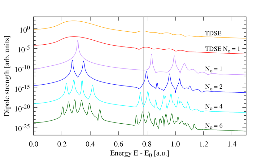
Figure 2: (color online) Linear response spectra obtained from TDRNOT calculations with different numbers of RNOs $N_{\mathrm{o}}$. For comparison also the exact TDSE result is plotted.

As stated before, the restriction to a finite number of RNOs introduces a truncation error. Truncation-error-free reference results for a given $N_{\mathrm{o}}$ can be obtained by diagonalization of the exact 1-RDM (from the TDSE). The resulting spectrum from only one truncation-error-free NO (labeled with TDSE $N_{\mathrm{o}}=1$) is also shown in Fig. 2. It almost completely coincides with the full exact result. One thus can conclude that almost all important information is already included in the first dominant RNO. However, due to the coupling between RNOs in the TDRNOT EOM all other RNOs are important during the propagation.

IV.3 H${}_{2}^{+}$ in intense laser fields

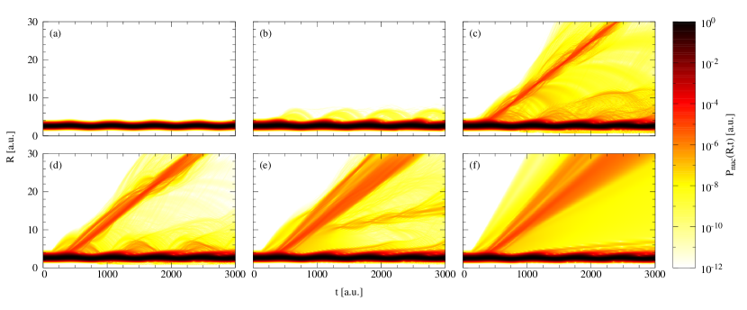
Figure 3: (color online) Time-dependent nuclear probability density upon the interaction with a $800$-nm four-cycle pulse with $I_{0}=10^{14}\,\mathrm{W}\mathrm{/}\mathrm{c}\mathrm{m}^{2}$. Again different numbers of orbitals were used: (a) $N_{\mathrm{o}}=1$, (b) $N_{\mathrm{o}}=2$, (c) $N_{\mathrm{o}}=4$, (d) $N_{\mathrm{o}}=8$, and (e) $N_{\mathrm{o}}=10$. With more RNOs included, the agreement with the exact result of the TDSE, given in panel (f), is considerably improved.

Many different processes influence the fragmentation dynamics of molecules subjected to intense laser fields, e.g., bond softening Bucksbaum et al. (1990), above-threshold dissociation (ATD) Giusti-Suzor et al. (1990), bond hardening or vibrational trapping Giusti-Suzor and Mies (1992), charge-resonance-enhanced ionization Zuo and Bandrauk (1995), and the “retroaction” due to the long-range Coulomb potential Waitz et al. (2016). We want to further benchmark TDRNOT by investigating its ability to describe non-perturbative phenomena far from equilibrium. As the theory is aiming to describe strong-field laser-matter interaction, we study the fragmentation of H${}_{2}^{+}$ upon the interaction with a short, intense laser pulse. Furthermore, HHG spectra are calculated.

IV.3.1 Dissociation and ionization

An infrared $800$-nm four-cycle pulse with a $\sin^{2}$-envelope and a peak intensity of $I_{0}=10^{14}\,\mathrm{W}\mathrm{/}\mathrm{c}\mathrm{m}^{2}$ was applied to the H${}_{2}^{+}$ model system. Upon the interaction with an intense laser pulse, fragmentation can occur due to dissociation or dissociative ionization (DI). In the latter case the removal of the electron leads to Coulomb explosion as the nuclei fly apart due to their Coulomb repulsion. In order to judge whether the different fragmentation processes can be reproduced with TDRNOT, we analyze the time-dependent nuclear probability density,

$$P_{\mathrm{nuc}}(R,t)=\int\mathrm{d}x\,|\Psi(x,R,t)|^{2}=\sum_{k}|\tilde{\eta}_{k}(R,t)|^{2}.$$ (26)

Figure 3 shows the logarithmically scaled, time-dependent nuclear probability density $P_{\mathrm{nuc}}(R,t)$ resulting from TDRNOT calculations. The TDSE reference result is included for comparison in Fig. 3f. In the latter figure a many fold jet-like structure becomes apparent, which can be attributed to dissociation. Due to ATD—the absorption of more photons than needed—dissociation channels with different kinetic energies of the fragments appear. In the TDH case $N_{\mathrm{o}}=1$, however, the time-dependent nuclear probability density shows no indication of dissociation at all (Fig. 3a). This erroneous behavior is due to the wrong shape of the effective nuclear potential again (see Fig. 1 in Ref. Kreibich et al. (2004)). Vibrations around the equilibrium internuclear distance are already reproduced though. A TDRNOT calculation with $N_{\mathrm{o}}=2$ does not lead to a much improved result. However, 4 RNOs are sufficient for reproducing dissociation, as the most prominent jet is clearly visible, although the broadening is not yet in good agreement with $P_{\mathrm{nuc}}(R,t)$ obtained from the TDSE. As expected, including more orbitals leads to a better agreement with the exact result. A second jet corresponding to dissociation upon the absorption of a different number of photons is already clearly visible in the $N_{\mathrm{o}}=8$ density, and with two more orbitals the broadening improves. However, an erroneous structure emerges at intermediate internuclear distances $10<R<20$, which vanishes with even more RNOs (not shown).

Figure 4: (color online) Energy spectra for nuclei and photoelectrons, calculated using the (extended) virtual detector method. (a) Kinetic-energy spectra of the nuclei for dissociation (blue) and DI (red). The vertical grey lines denote $2\omega$, $3\omega$, and $4\omega$ absorption from the vibrational ground state. (b) TDRNOT photoelectron spectrum for 10 RNOs per degree of freedom (red, dashed) compared to the exact result from the TDSE (orange, solid).

The kinetic energy release (KER) in the nuclear fragments for dissociation and DI can be calculated from the RNOs by means of the virtual detector method Feuerstein and Thumm (2003b, a). To that end we reconstruct the wavefunction from the RNOs and then follow Ref. Feuerstein and Thumm (2003a). The resulting KER spectra obtained with 10 RNOs per degree of freedom are compared with the corresponding TDSE benchmark results in Fig. 4a.

Regarding dissociation, multiple peaks at energies $E_{\mathrm{kin}}<0.2$ are observed. The most distinct peaks are separated by roughly the photon energy and can be assigned to three and four-photon ATD, respectively. These processes were found to be dominant also for longer pulses of the same wavelength and intensity Peng et al. (2005). The expected positions of the peaks (using the BO-approximation and assuming the vibrational ground state) in the spectrum can be calculated using a simple energy conservation formula Chelkowski et al. (1998). These positions are depicted as vertical gray lines in Fig. 4a. The spectrum obtained from the TDRNOT calculation has a structure similar to the exact one—heights and positions of the peaks coincide approximately with the exact results. However, in the TDRNOT spectrum several discrete peaks are visible for the three-photon dissociation instead of the broad, continuous energy distribution in the exact spectrum. Moreover, there are discrepancies for lower energies, and the two-photon dissociation is missing completely.

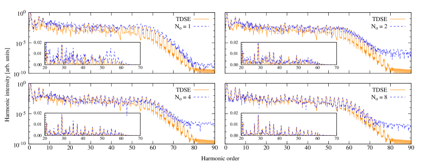
Figure 5: (color online) HHG spectra calculated with TDRNOT using 1, 2, 4, and 8 RNOs per degree of freedom compared to the exact spectrum obtained from the TDSE. The insets show a section of each spectrum plotted on a linear scale.

The KER spectrum in the case of DI is, as the Coulomb energy is released, centered around higher energies $E_{\mathrm{kin}}>0.2$. Note the different scaling of the ordinate as the ionization yield is several orders of magnitude below the dissociation yield. There are slight deviations of TDRNOT from the exact result—the spectrum obtained from TDRNOT is shifted towards lower energies—but the general structure of the spectrum is reproduced.

Furthermore, in the case of DI, we calculate electronic kinetic-energy spectra using the extended virtual detector method Wang et al. (2013). Starting from the virtual detectors, classical trajectories are calculated in order to obtain the final momentum of the electron at the end of the laser pulse. The results are presented in Fig. 4b. For both, the TDRNOT and the TDSE results, a modulation in the yield, depending on $E_{\mathrm{kin}}^{\mathrm{el}}$ is visible. This can be attributed to the interference of quantum trajectories starting at different ionization times, which lead to the same final momentum Milošević et al. (2006); Arbó et al. (2010). In the case of the electronic kinetic-energy spectrum, the agreement between the results from a TDRNOT calculation with $N_{\mathrm{o}}=10$ and the exact result is clearly better than for the KER spectra. This shows that different minimum numbers of RNOs are required, depending on the observable to calculate.

IV.3.2 HHG spectra

Harmonic spectra are obtained by Fourier transforming the time-dependent dipole acceleration $\ddot{d}(t)$ Burnett et al. (1992), which is given by

$$\mu_{\mathrm{e}}\,\ddot{d}(t)=\braket{\Psi(t)}{-\nabla\hat{V}_{\mathrm{en}}+q_{\mathrm{e}}\,E(t)}{\Psi(t)}.$$ (27)

An $800$-nm 10-cycle pulse with $\sin^{2}$-shaped on- and off-ramping over two cycles was employed. The peak intensity of the laser pulse was $I_{0}=3.0\times 10^{14}\,\mathrm{W}\mathrm{/}\mathrm{c}\mathrm{m}^{2}$. In Fig. 5, TDRNOT HHG spectra, calculated using 1 to 8 RNOs per degree of freedom, are compared to the exact TDSE spectrum. In the inset, a part of the spectrum is plotted on a linear scale.

With only 1 RNO the position of the cut-off is already in good agreement with the exact result. However, the shape of individual peaks, especially at high harmonic order, is completely wrong. The TDRNOT calculation with $N_{\mathrm{o}}=2$ exhibits erroneous peaks in addition to the peaks at the odd harmonics, especially pronounced in the region beyond the cut-off. When adding more RNOs the quantitative agreement improves, and the wrong peaks vanish. A similar improvement with increasing number of single-particle functions has been reported for calculations using a MCTDH approach Jhala and Lein (2010). For $N_{\mathrm{o}}=8$ the height and the shape of the peaks are well reproduced up to the 60th harmonic order. At very high harmonic orders some deviations in the spectra are still visible, and the noise level of the TDRNOT results is two orders of magnitude higher than for the TDSE. A similar behavior was observed for HHG in a model He atom Brics et al. (2016). On a linear scale, as often used in experiments, the agreement is excellent and clearly improves with increasing $N_{\mathrm{o}}$ (see insets in Fig. 5).

V Conclusion

We have investigated the performance of time-dependent renormalized-natural-orbital theory (TDRNOT) when applied to the simplest multi-component system exhibiting electron-nuclear correlation, i.e., H${}_{2}^{+}$. Different types of renormalized natural orbitals (RNOs), describing the electronic and the nuclear component, were introduced, and their coupled EOM derived. As in the case of helium investigated earlier no approximations concerning the expansion of the time-dependent two-body density matrix need to be made.

In order to benchmark the theory the ground state of a one-dimensional H${}_{2}^{+}$ model system and linear response spectra were calculated using TDRNOT. While an excellent agreement with the exact ground state energy was achieved with very few orbitals, the linear response spectra were plagued by multiple sharp peaks that only for very many orbitals would reproduce the correct, broad structure caused by bound-continuum transitions. This unpleasant feature is caused by the restriction to a finite number of orbitals, which introduces a truncation error. Future work will be devoted to improve on that aspect of TDRNOT.

Finally, TDRNOT was applied to H${}_{2}^{+}$ interacting with a short, intense laser pulse. The time evolution of the nuclear probability density was studied, and features indicating different fragmentation processes were identified. It was found that TDRNOT is able to reproduce dissociation and Coulomb explosion and the corresponding kinetic-energy-release spectra if enough RNOs are taken into account. The same applies to high-harmonics spectra where 8 RNOs were found yield very good agreement with the benchmark result from the time-dependent Schrödinger equation.