Higgs vacuum metastability in primordial inflation, preheating, and reheating

Abstract

Current measurements of the Higgs boson mass and top Yukawa coupling suggest that the effective Higgs potential develops an instability below the Planck scale. If the energy scale of inflation is as high as the GUT scale, inflationary quantum fluctuations of the Higgs field can easily destabilize the standard electroweak vacuum and produce a lot of AdS domains. This destabilization during inflation can be avoided if a relatively large nonminimal Higgs-gravity or inflaton-Higgs coupling is introduced. Such couplings generate a large effective mass term for the Higgs, which can raise the effective Higgs potential and suppress the vacuum fluctuation of the Higgs field. After primordial inflation, however, such effective masses drops rapidly and the nonminimal Higgs-gravity or inflaton-Higgs coupling can cause large fluctuations of the Higgs field to be generated via parametric resonance, thus producing AdS domains in the preheating stage. Furthermore, thermal fluctuations of the Higgs field cannot be neglected in the proceeding reheating epoch. We discuss the Higgs vacuum fluctuations during inflation, preheating, and reheating, and show that the Higgs metastability problem is severe unless the energy scale of the inflaton potential is much lower than the GUT scale.

I Introduction

With the discovery of the Higgs boson at the LHC, the standard model has been completed, and elementary particle physics has entered a new era. The recent measurements of the Higgs boson mass, $m_{h}=125.09\ \pm\ 0.21\ ({\rm stat})\ \pm\ 0.11\ ({\rm syst})\ {\rm GeV}$  Aad et al. (2015, 2013); Chatrchyan et al. (2014); Giardino et al. (2014) and top quark mass, $m_{t}=173.34\pm 0.27\ ({\rm stat})\pm 0.71\ ({\rm syst})\ {\rm GeV}$ ATLAS et al. (2014) suggest that the running of the quartic Higgs self-coupling $\lambda$ becomes negative, and the effective Higgs potential becomes unstable at the scale $\Lambda_{I}=10^{10}\sim 10^{11}\ {\rm GeV}$ Buttazzo et al. (2013).

If the effective Higgs potential is unstable below the Planck scale, our electroweak vacuum is metastable and should eventually decay into the true vacuum through quantum tunneling Kobzarev, Okun, and Voloshin (1975); Coleman (1977); Callan and Coleman (1977). The timescale for this decay, however, is longer than the age of the Universe, so it was thought that the Higgs vacuum metastability does not phenomenologically have any significant impact on the observed Universe Degrassi et al. (2012); Isidori, Ridolfi, and Strumia (2001); Ellis et al. (2009); Elias-Miro et al. (2012). However, recently it has been argued that the electroweak vacuum instability during inflation or at the end of inflation might threaten the existence of the Universe Espinosa, Giudice, and Riotto (2008); Fairbairn and Hogan (2014); Kobakhidze and Spencer-Smith (2013); Lebedev and Westphal (2013); Kobakhidze and Spencer-Smith (2013); Enqvist, Meriniemi, and Nurmi (2013); Herranen et al. (2014); Kobakhidze and Spencer-Smith (2014); Kamada (2015); Enqvist, Meriniemi, and Nurmi (2014); Hook et al. (2015); Kearney, Yoo, and Zurek (2015); Espinosa et al. (2015); Gross, Lebedev, and Zatta (2015); Herranen et al. (2015); Ema, Mukaida, and Nakayama (2016). Stochastic quantum fluctuations produced during inflation can cause the Higgs field value to grow as

$$\left<{h}^{2}\right>\simeq\frac{{H}^{3}t}{4{\pi}^{2}},$$ (1)

where $h$ is the value of the Higgs and $H$ is the Hubble expansion rate (or the Hubble scale). If the Higgs field evolves beyond the instability scale $\Lambda_{I}$ before the end of inflation, the Higgs field classically rolls down into the true vacuum and Anti-de Sitter (AdS) domains are formed, which is potentially catastrophic.

Not all AdS domains generated during inflation threaten the existence of our Universe Hook et al. (2015); Kearney, Yoo, and Zurek (2015); Espinosa et al. (2015), with the significance highly depending on the number and the evolution of the AdS domains. In Ref.Espinosa et al. (2015), the authors discussed how AdS domains evolve both during inflation and after the end of inflation. The Higgs AdS domains can either shrink or expand, eating other regions of the electroweak vacuum. Although high-energy-scale inflation can lead to the generation of more expanding AdS domains during inflation, such domains never take over all of the inflationary dS space, because the inflationary expansion always overcomes the expansion of the AdS domains. However, after the inflationary epoch, although some AdS domains harmlessly shrink, others expand and devour our whole Universe. This indicates that the existence of AdS domains in our observable universe is catastrophic, and so in this paper we focus on the conditions for them not to be generated.

The generation of Higgs AdS domains during inflation can be suppressed by introducing a relatively large nonminimal Higgs-gravity or inflaton-Higgs coupling. Such couplings give rise to large inflationary effective mass terms, which raise the effective Higgs potential and weaken the Higgs vacuum fluctuations Espinosa et al. (2015); Lebedev and Westphal (2013); Kamada (2015). However, at the end of the inflation, such mass terms drops rapidly, and become ineffective for stabilizing the Higgs field Kamada (2015). Nonminimal Higgs-gravity or inflaton-Higgs coupling can also cause large Higgs fluctuations to be generated via parametric resonance Herranen et al. (2015); Ema, Mukaida, and Nakayama (2016), thus producing a lot of AdS domains in the preheating stage. Moreover, thermal Higgs fluctuations are not negligible in the reheating epoch after inflation. In this paper, we analyse the vacuum fluctuations of the Higgs field during inflation, preheating, and reheating and show that the Higgs metastability is a serious problem in the inflationary Universe unless the energy scale of the inflaton potential is much lower than the GUT scale or the effective Higgs potential is stabilized below the Planck scale. In this paper, we use the reduced Planck mass, $M_{\rm pl}=2.4\times 10^{18}\ {\rm GeV}$.

II Inflationary Higgs fluctuations and Higgs AdS domains

In this section, we discuss the evolution of the massless Higgs field during inflation using the Fokker-Planck equation, and determine the probability that Higgs AdS domains are formed. In the large-field regime $h\gg v$, where $v=246\ {\rm GeV}$, the effective Higgs potential can be approximated by the following Renormalization Group (RG) improved tree-level expression,

$$V_{\rm eff}\left(h\right)=\frac{\lambda_{\rm eff}\left(h\right)}{4}h^{4},$$ (2)

where $\lambda_{\rm eff}\left(h\right)$ is the effective self-coupling including the RG improved couplings, the one-loop corrections. The instability scale $\Lambda_{I}$ can be defined as the effective self-coupling $\lambda_{\rm eff}\left(h\right)$ becomes negative at the scale. In the RG improved effective Higgs potential, the instability scale is $\Lambda_{I}\simeq h_{\rm max}$ where $h_{\rm max}$ defined as $V_{\rm eff}\left(h\right)$ takes its maximal value.

When the Hubble scale $H$ is smaller than the Higgs field value at the maximum of the effective Higgs potential, $h_{\rm max}$, the Higgs field can tunnel into the true vacuum via the Coleman-de Luccia instanton Coleman and De Luccia (1980). If the Hubble rate is as large as the maximal Higgs field value $h_{\rm max}$, the transition is dominated by the Hawking-Moss instanton Hawking and Moss (1982). The transition probability of the Higgs field during inflation can also be obtained by statistical approaches using the Fokker-Planck equation, with the result being approximately equal to that obtained using the Hawking-Moss instanton Linde (1992).

The Fokker-Planck equation describes the evolution of the probability $P\left(h,t\right)$ that the Higgs takes the value $h$ in one Hubble horizon-size region at cosmic time $t$, and takes the following form

$$\frac{\partial{P}}{\partial t}=\frac{\partial^{2}}{\partial h^{2}}\left(\frac{{H}^{3}}{8{\pi}^{2}}P\right)+\frac{\partial}{\partial h}\left(\frac{V_{\rm eff}^{\prime}\left(h\right)}{3H}{P}\right),$$ (3)

where the prime ^′ denotes the derivative with respect to the field, i.e. $V^{\prime}_{\rm eff}(h)=\frac{dV_{\rm eff}}{dh}$. According to Ref.Espinosa et al. (2015), we may ignore the gradient of the effective Higgs potential $V_{\rm eff}^{\prime}\left(h\right)$, with assuming that the field value is $h=0$ at $t=0$, which gives,

$$P\left(h,t\right)=\sqrt{\frac{2{\pi}}{{H}^{3}t}}\exp\left(-\frac{2{{\pi}^{2}}}{{H}^{3}t}{h}^{2}\right).$$ (4)

During inflation, if the Higgs in some region evolves to values larger than $\Lambda_{I}$, then it will roll into the true vacuum and a potentially dangerous AdS region will be formed. The survival probability of the electroweak vacuum at the end of inflation is estimated to be Espinosa, Giudice, and Riotto (2008); Espinosa et al. (2015)

$${P}\left(h<\Lambda_{I},N_{\rm tot}\right) \equiv \int_{-\Lambda_{I}}^{\Lambda_{I}}{dh\ P\left(h,t_{\rm end}\right)},$$ (5)

$$= {\rm erf}\left(\frac{\sqrt{2}\pi\Lambda_{I}}{H\sqrt{N_{\rm tot}}}\right),$$ (6)

where $t_{\rm end}$ denotes the time at the end of inflation, $N_{\rm tot}$ is the total $e$-folding number, defined as $N_{\rm tot}=H\cdot t_{\rm end}$, and ${\rm erf}\left(x\right)$ is the error function, which for $x\gg 1$ is approximately given by

$${\rm erf}\left(x\right)\simeq 1-\frac{1}{\sqrt{\pi}x}{e}^{-{x}^{2}}.$$ (7)

Note that the total e-folding number can be much larger than the observable e-folding number $N_{\rm hor}$, which is the number of e-foldings before the end of inflation that the largest observable scales left the Horizon, i.e. we could have ${N}_{\rm tot}\gg{N}_{\rm hor}$. This implies that our observable universe is only part of the whole Universe.

$P(h,t)$ in the Fokker-Planck equation describes the probability distribution of the Higgs in one horizon-sized region Nambu (1989); Nambu and Sasaki (1989). Inflation produces many such regions, and our observable Universe contains $e^{3N_{\rm hor}}$ of them. As such, the survival probability can be estimated as

$$\left\{{P}\left(h<\Lambda_{I},N_{\rm tot}\right)\right\}^{{e}^{3N_{\rm hor}}}>\frac{1}{2},$$ (8)

which, using (6) and (7), can be approximately re-written as

$$\left\{1-\frac{H\sqrt{N_{\rm tot}}}{\pi\sqrt{2\pi}\ \Lambda_{I}}{e}^{-{\frac{2{\pi}^{2}\Lambda_{I}^{2}}{{H}^{2}N_{\rm tot}}}}\right\}^{{e}^{3N_{\rm hor}}}>\frac{1}{2}.$$ (9)

If we set $N_{\rm hor}=60$ and $N_{\rm tot}=10^{3}$ in (9), we obtain the following upper bound on the Hubble scale,

$$\frac{H}{\Lambda_{I}}<1.1\times 10^{-2}.$$ (10)

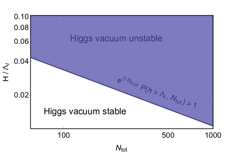
Figure 1: Plot of the upper bound on $H/\Lambda_{I}$ as a function of the total $e$-folding number $N_{\rm tot}$, as determined by (13). We set $N_{\rm hor}=60$ and $60\leq N_{\rm tot}$.

Alternatively, we can restrict $H$ by using the probability that the field rolls down into the true vacuum at the end of inflation, ${P}\left(h>\Lambda_{I},N_{\rm tot}\right)$, which is given as

$${P}\left(h>\Lambda_{I},N_{\rm tot}\right) = 1-{P}\left(h<\Lambda_{I},N_{\rm tot}\right),$$ (11)

$$\simeq \frac{H\sqrt{N_{\rm tot}}}{\pi\sqrt{2\pi}\ \Lambda_{I}}{e}^{-{\frac{2{\pi}^{2}\Lambda_{I}^{2}}{{H}^{2}N_{\rm tot}}}}.$$ (12)

Multiplying this by ${e}^{3N_{\rm hor}}$ gives the number of AdS domains in the local region corresponding to our observable Universe. As such, the condition that there be no AdS regions within the current horizon is expressed as

$${e}^{3N_{\rm hor}}{P}\left(h>\Lambda_{I},N_{\rm tot}\right)<1,$$ (13)

which can be approximated as

$$\scalebox{0.9}{$\displaystyle{e}^{3N_{\rm hor}}{P}\left(h>\Lambda_{I},N_{\rm tot}\right)=\frac{H\sqrt{N_{\rm tot}}}{\pi\sqrt{2\pi}\ \Lambda_{I}}{e}^{3N_{\rm hor}-{\frac{2{\pi}^{2}\Lambda_{I}^{2}}{{H}^{2}N_{\rm tot}}}}$}.$$ (14)

Therefore, we have the upper bound on the Hubble scale,

$$\frac{H}{\Lambda_{I}}<\sqrt{\frac{2{\pi}^{2}}{3N_{\rm hor}N_{\rm tot}}}.$$ (15)

If we take $N_{\rm hor}=60$ and $N_{\rm tot}=10^{3}$ in (14), the upper bound on the Hubble scale is numerically found to be

$$\frac{H}{\Lambda_{I}}<1.1\times 10^{-2}.$$ (16)

In Fig. 1, we plot the upper bound on $H/\Lambda_{I}$ as a function of the total $e$-folding number $N_{\rm tot}$, as determined by (13). We assume that $N_{\rm hor}=60$ and that the total $e$-folding number is greater than $N_{\rm hor}$, i.e. $60\leq N_{\rm tot}$. It is natural to consider that the total $e$-folding number $N_{\rm tot}$ may be huge, due to the stochastic nature of inflation, and the inflationary Higgs vacuum fluctuations grow as time goes by. Consequently, requiring the Higgs vacuum to remain stable throughout inflation puts tight constraints on the Hubble scale during inflation.

Although the AdS domains impact on the existence of our observable universe, the expansion of AdS domains never takes over the expansion of inflationary dS space Espinosa et al. (2015), and therefore, it is impossible that one AdS domain terminates the inflation on all the space of the Universe. However, If the proportion of non-inflating domains or the AdS domains dominates all the space of the Universe Kearney, Yoo, and Zurek (2015); Sekino, Shenker, and Susskind (2010), the inflating space would crack, and inflation comes to an end.

III Inflationary Higgs vacuum fluctuations during inflation

In the previous section we discussed the massless Higgs vacuum fluctuations during inflation, and by solving the Fokker-Planck equation we were able to determine the probability for the formation of Higgs AdS domains. In general, the inflationary Higgs fluctuations become as large as the Hubble scale $H$ during inflation. However, if the Higgs field has a large effective mass, the Higgs vacuum fluctuations are suppressed during inflation. Field fluctuations in the massive case, particularly in the case where $m>3H/2$, have often been discussed using different descriptions in the literature. In this section we introduce mass terms for the Higgs field, determine its fluctuations, calculate the probability for the formation of Higgs AdS domains and obtain constraints on the model parameters by requiring consistency with observations.

III.1 Fluctuations of light Higgs field

The FLRW metric is given by

$$g_{\mu\nu}={\rm diag}\left(-1,\frac{{a}^{2}\left(t\right)}{1-K{r}^{2}},{a}^{2}\left(t\right){r}^{2},{a}^{2}\left(t\right){r}^{2}\sin^{2}{\theta}\right),$$ (17)

where $K$ is the curvature constant and $a=a(t)$ is the scale factor. For simplicity we will take $K=0$. Then, the scalar curvature is obtained as

$$R=6\left[{\left(\frac{\dot{a}}{a}\right)}^{2}+\left(\frac{\ddot{a}}{a}\right)\right].$$ (18)

In a de Sitter Universe where $a\propto e^{Ht}$, the Ricci scalar is estimated to be $R\simeq 12H^{2}$. We assume that the total scalar potential for the inflaton and Higgs is given as follows

$$V\left(\phi,h\right)=V_{\rm inf}\left(\phi\right)+V_{\rm eff}\left(h\right)+\frac{1}{2}\xi h^{2}R+\frac{1}{2}g^{2}\phi^{2}h^{2},$$ (19)

where $\phi$ is the inflation field, $\xi$ is the nonminimal Higgs-gravity coupling constant, and $g$ is the coupling constant between $h$ and $\phi$. The Klein-Gordon equation for Fourier modes of the Higgs field is given as

$${\delta\ddot{h}}_{k}+3H{\delta\dot{h}}_{k}+\left(\frac{k^{2}}{a^{2}}+\xi R+g^{2}\phi^{2}\right){\delta{h}}_{k}=0,$$ (20)

where we have assumed that we can neglect the contribution from $V_{\rm eff}(h)$ in comparison with the other terms. A finite value of $\xi$ or $g$ therefore generates an effective Higgs mass, which during inflation is approximately given as

$$m_{\rm eff}^{2}\simeq 12H^{2}\xi+g^{2}\phi^{2}.$$ (21)

The additional Higgs mass can raise the effective Higgs potential and suppress the vacuum fluctuation of the Higgs field. The maximum of the Higgs potential gets shifted to larger values of $h$.

We introduce the redefined field $\delta\sigma_{k}$ which is related to $\delta h_{k}$ as

$$\delta\sigma_{k}=a\delta{h}_{k}.$$ (22)

The Klein-Gordon equation for $\delta\sigma_{k}$ takes the form

$$\delta\sigma_{k}^{\prime\prime}+\left(k^{2}-\frac{1}{\tau^{2}}\left(\nu^{2}-\frac{1}{4}\right)\right)\delta\sigma_{k}=0,$$ (23)

where the conformal time has been introduced and is defined as $d\tau=dt/a$, and $\nu$ is defined to be

$$\nu=\sqrt{\frac{9}{4}-\frac{m_{\rm eff}^{2}}{H^{2}}}.$$ (24)

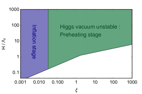
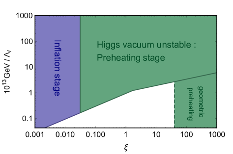
(a)  nonminimal coupling $\xi$ (b)  nonminimal coupling $\xi$

Figure 2: Constraints on $H/\Lambda_{I}$ as a function of the nonminimal coupling $\xi$. We have plotted the lines shown in (38) and (52). We took the effective mass to be $m_{\rm eff}=\sqrt{12\xi}H$ and set $N_{\rm hor}=N_{\rm tot}=60$. In the left panel we neglect the constraint coming from the parametric amplification of the Higgs field in order to remove model-dependence. On the other hand, in the right panel we include the constraint coming from broad resonance during the preheating stage, taking the quadratic chaotic inflation model $V_{\rm inf}\left(\phi\right)\simeq\frac{1}{2}m_{\phi}^{2}\phi^{2}$ and the Hubble scale $H\simeq 10^{13}\ {\rm GeV}$ as an example.

The general solution of Eq. (23) is expressed as

$$\delta\sigma_{k}=\sqrt{-\tau}\left[{c}_{1}{H}_{\nu}^{\left(1\right)}\left(-k\tau\right)+{c}_{2}{H}_{\nu}^{\left(2\right)}\left(-k\tau\right)\right],$$ (25)

where ${H}_{\nu\in C}^{\left(1\right)}\left(x\right)$ and ${H}_{\nu\in C}^{\left(2\right)}\left(x\right)$ are Hankel functions of the first and second kind. In order to determine the coefficients $c_{1}$ and $c_{2}$, in the ultraviolet regime $\left(-k\tau\gg 1\right)$ we match the solution with the postivie-frequency plane-wave solution in flat spacetime, $e^{-ik\tau}/\sqrt{2k}$, which gives

$$c_{1}=\frac{\pi}{2}e^{i\left(\nu+\frac{1}{2}\right)\frac{\pi}{2}},\quad c_{2}=0.$$ (26)

The choice of a particular set of coefficients $c_{1},c_{2}$ is equivalent to choosing the vacuum Birrell and Davies (1984). On super-horizon scales $\left(-k\tau\ll 1\right)$, the re-scaled mode functions of the Higgs take the form

$$\delta\sigma_{k} = \frac{\pi}{2}e^{i\left(\nu+\frac{1}{2}\right)\frac{\pi}{2}}\sqrt{-\tau}{H}_{\nu}^{\left(1\right)}\left(-k\tau\right),$$ (27)

$$= e^{i\left(\nu-\frac{1}{2}\right)\frac{\pi}{2}}2^{\nu-\frac{3}{2}}\frac{\Gamma\left(\nu\right)}{\Gamma\left(3/2\right)}\frac{1}{\sqrt{2k}}{\left(-k\tau\right)}^{\frac{1}{2}-\nu}.$$ (28)

If we consider the case where the Higgs mass is light, i.e. $m_{\rm eff}\leq 3H/2$, the absolute value of $\delta h_{k}$ is given as

$$\left|\delta h_{k}\right| = \frac{H}{\sqrt{2k^{3}}}2^{\nu-\frac{3}{2}}\frac{\Gamma\left(\nu\right)}{\Gamma\left(3/2\right)}\frac{k}{aH}{\left(\frac{k}{aH}\right)}^{\frac{1}{2}-\nu},$$ (29)

$$\simeq \frac{H}{\sqrt{2k^{3}}}{\left(\frac{k}{aH}\right)}^{\frac{3}{2}-\nu}.$$

Integrating over super-horizon modes we obtain the variance of the Higgs field fluctuations a

$$\left<{h}^{2}\right> = \int_{H}^{aH}{{\left|\delta h_{k}\right|}^{2}\frac{d^{3}k}{\left(2\pi\right)^{3}}},$$ (30)

$$\simeq \frac{3{H}^{4}}{8{\pi}^{2}m_{\rm eff}^{2}}\quad(m_{\rm eff}\ll 3H/2).$$ (31)

Next we assume that the Higgs probability distribution function is Gaussian, i.e.

$$P\left(h,t\right)=\frac{1}{\sqrt{2{\pi}\left<{h}^{2}\right>}}\exp\left(-\frac{h^{2}}{2\left<{h}^{2}\right>}\right).$$ (32)

By using Eq. (5), the probability that the standard electroweak vacuum survives can be obtained as

$${P}\left(h<{h}_{\rm max},N_{\rm tot}\right) \equiv \int_{-{h}_{\rm max}}^{{h}_{\rm max}}{dh\ P\left(h,t_{\rm end}\right)},$$ (33)

$$= {\rm erf}\left(\frac{{h}_{\rm max}}{\sqrt{2\left<{h}^{2}\right>}}\right).$$ (34)

On the other hand, the probability that the Higgs falls into the true vacuum is expressed as

$${P}\left(h>{h}_{\rm max},N_{\rm tot}\right) = 1-{\rm erf}\left(\frac{{h}_{\rm max}}{\sqrt{2\left<{h}^{2}\right>}}\right),$$ (35)

$$\simeq \sqrt{\frac{2}{\pi}}\frac{\sqrt{\left<{h}^{2}\right>}}{{h}_{\rm max}}e^{-\frac{{h}_{\rm max}^{2}}{2\left<{h}^{2}\right>}}.$$ (36)

Imposing the condition shown in (13), we obtain the relation

$$\frac{\left<{h}^{2}\right>}{{h}_{\rm max}^{2}}<\frac{1}{6N_{\rm hor}}.$$ (37)

If we substitute $\langle h^{2}\rangle$ from Eq. (31) into this relation, we find the upper bound on $H$ to be

$$\frac{H}{{h}_{\rm max}}<\frac{2{\pi}m_{\rm eff}}{3H\sqrt{N_{\rm hor}}},$$ (38)

which is the same as the constraint given in Ref.Espinosa et al. (2015). We plot this line in Fig. 2, where we assume $h_{\rm max}\sim\Lambda_{I}$ because of the small nonminimal coupling $\xi$ and it is labelled by “Inflation Stage”.

III.2 Fluctuations of Massive Higgs field

In this subsection, we consider the case of a large effective Higgs mass, namely $m_{\rm eff}>3H/2$. We define $\tilde{\nu}$ as

$$\tilde{\nu}=\sqrt{\frac{m_{\rm eff}^{2}}{H^{2}}-\frac{9}{4}}.$$ (39)

On super-horizon scales, the re-scaled Higgs fluctuations are given by

$$\delta\sigma_{k}=\frac{\pi}{2}e^{i\left(i\tilde{\nu}+\frac{1}{2}\right)\frac{\pi}{2}}\sqrt{-\tau}{H}_{i\tilde{\nu}}^{\left(1\right)}\left(-k\tau\right).$$ (40)

The absolute value of $\delta\sigma_{k}$ is obtained as

$$\left|\delta\sigma_{k}\right|\simeq\frac{1}{\sqrt{2k}}\left(-k\tau\right)^{1/2}\frac{{e}^{\frac{\pi}{2}\tilde{\nu}}}{\sqrt{2\pi}\tilde{\nu}}\left|\Gamma\left(1-i\tilde{\nu}\right)\right|.$$ (41)

Using the relation ${\left|\Gamma\left(1-iy\right)\right|}^{2}=\pi y/\sinh{\left(\pi y\right)}$, the fluctuations of the massive Higgs field are estimated to be

$$\left|\delta h_{k}\right|^{2}\simeq\frac{1}{2a^{3}\tilde{\nu}H}.$$ (42)

As such, the variance of the vacuum fluctuations during inflation is given as

$$\left<{h}^{2}\right> = \int_{H}^{aH}{{\left|\delta h_{k}\right|}^{2}\frac{d^{3}k}{\left(2\pi\right)^{3}}}\simeq\frac{H^{2}}{12{\pi}^{2}\tilde{\nu}},$$ (43)

$$\approx \frac{H^{3}}{12{\pi}^{2}m_{\rm eff}}.$$ (44)

Inflationary effective mass terms thus lift the effective Higgs potential and suppress the Higgs vacuum fluctuations. Substituting the above result into (37), in the case of a massive Higgs field the requirement that our observable Universe contains no AdS domains gives us the condition

$$\frac{H}{{h}_{\rm max}}<\sqrt{\frac{2{\pi}^{2}{m}_{\rm eff}}{H{N}_{\rm hor}}}.$$ (45)

The constraint on the nonminimal coupling $\xi$ can be estimated by those conditions shown in (38) and (45). If we assume $m_{\rm eff}=\sqrt{12\xi}H$, we obtain a lower bound on the nonminimal coupling as $\xi>0.03$ using the fact that $h_{\rm max}\simeq 10m_{\rm eff}$. This constraint corresponds to the vertical line in Fig. 2. In the case of inflaton-Higgs coupling, where $m_{\rm eff}=g\phi$, we can similarly obtain a constraint on $g$, but it will depend on the inflaton field value $\phi$ and the Hubble scale $H$.

Whilst inflationary effective masses can prevent the Higgs from evolving into the true vacuum during inflation, after inflation they become ineffective, and the Higgs field fluctuations generated as a result of resonant preheating may destabilize the standard electroweak vacuum. We will discuss this problem in the next section.

IV Higgs fluctuations after inflation and during the preheating stage

After the end of inflation, the inflaton field $\phi$ oscillates near the minimum of its potential and produces a huge amount of elementary particles that interact with each other and eventually form a thermal plasma. The reheating process is generally classified into several stages. In the first stage, the classical, coherently-oscillating inflaton field $\phi$ may give rise to the production of massive bosons due to parametric resonance. In most cases, this first stage occurs extremely rapidly. This nonthermal period is called preheating Kofman, Linde, and Starobinsky (1997), and is different from the subsequent stages of reheating and thermalization. Parametric resonance in the preheating stage may sometimes produce topological defects or lead to nonthermal phase transitions Kofman, Linde, and Starobinsky (1996).

In Ref.Herranen et al. (2015), the authors discussed the resonant production of Higgs fluctuations after inflation in the case that the Higgs is non-minimally coupled to gravity. However, the preheating dynamics is extremely complicated, and it is difficult to estimate analytically the Higgs vacuum fluctuations during the preheating stage. In this section, we numerically analyse the Higgs fluctuations after inflation and during the preheating stage. After inflation, the re-scaled Higgs mode solution is no longer given by Eq. (25). Instead, we use the WKB approximation and obtain the variance of the massive Higgs fluctuations which correspond with the result given by Eq. (44).

The Klein-Gordon equation for $k$-modes of the Higgs field is given as

$${\delta\ddot{h}}_{k}+3H{\delta\dot{h}}_{k}+\left(\frac{k^{2}}{a^{2}}+m_{\rm eff}^{2}\right){\delta{h}}_{k}=0,$$ (46)

which can be re-written in the useful form

$$\begin{split}\frac{d^{2}\left(a^{3/2}{\delta{h}}_{k}\right)}{dt^{2}}+\left(\frac{k^{2}}{a^{2}}+m_{\rm eff}^{2}-\frac{9}{4}H^{2}-\frac{3}{2}\dot{H}\right)\left(a^{3/2}{\delta{h}}_{k}\right)=0.\end{split}$$ (47)

If we consider the massive Higgs field case, i.e. $m_{\rm eff}>3H/2$, then the Higgs mode functions are given by

$${\delta{h}}_{k}\simeq\frac{e^{-i\omega_{k}\left(t\right)\cdot t}}{a^{3/2}\sqrt{2\omega_{k}\left(t\right)}}.$$ (48)

where $\omega_{k}^{2}\simeq\frac{k^{2}}{a^{2}}+m_{\rm eff}^{2}$ and we have assumed the adiabatic condition $\dot{\omega}_{k}\left(t\right)/\omega_{k}^{2}\left(t\right)\ll 1$ is satisfied, and ${\omega}_{k}^{2}\left(t\right)>0$. As such, the amplitude $\left|{\delta{h}}_{k}\right|^{2}$ after inflation is estimated to be Jin and Tsujikawa (2006)

$$\left|{\delta{h}}_{k}\right|^{2}\simeq\frac{1}{2a^{3}\omega_{k}}.$$ (49)

Hence, the variance of the massive Higgs fluctuations which are outside the Hubble radius after inflation is given as

$$\left<{h}^{2}\right>_{\rm end} = \frac{1}{2\pi^{2}}\int_{0}^{a_{\rm end}H_{\rm end}}k^{2}{{\left|\delta h_{k}\right|}^{2}dk},$$ (50)

$$\simeq \frac{H_{\rm end}^{3}}{12{\pi}^{2}m_{\rm eff}}.$$ (51)

This can be used as an estimate for the minimum amplitude of the homogeneous Higgs field after inflation. The above Higgs fluctuations are consistent with the result given by Eq. (44) and exponentially amplified by parametric resonance. If we substitute Eq. (51) into (37), we obtain the constraint

$$\frac{H_{\rm end}}{\Lambda_{I}}<\sqrt{\frac{2\pi^{2}m_{\rm eff}}{N_{\rm hor}H_{\rm end}}}.$$ (52)

Note that the effective mass ( $m_{\rm eff}\simeq\sqrt{\xi R\left(t\right)}$  or $m_{\rm eff}\simeq g\phi\left(t\right)$) decreases and sometimes disappears during the preheating period. Therefore, the effective mass cannot stabilizes the effective Higgs potential $V_{\rm eff}\left(h\right)$, and we can assume $h_{\rm max}\simeq\Lambda_{I}$.

Let us consider the amplification of the Higgs vacuum fluctuations via parametric resonance. For simplicity, we consider chaotic inflation with a quadratic potential as an example, i.e.

$$V_{\rm inf}\left(\phi\right)=\frac{1}{2}m_{\phi}^{2}\phi^{2},$$ (53)

where $m_{\phi}\simeq 7\times 10^{-6}M_{\rm pl}$. In the chaotic inflation scenario, inflation occurs at super-Planckian field values, $\phi>5M_{\rm pl}$. Primordial density perturbations relevant for the CMB are produced at around $\phi\sim 15M_{\rm pl}$, and inflation terminates at $\phi\sim 3M_{\rm pl}$. After inflation, the inflaton field oscillates as

$$\phi\left(t\right) = \Phi\left(t\right)\sin{m_{\phi}t},$$ (54)

$$\Phi\left(t\right) = \sqrt{\frac{8}{3}}\frac{M_{\rm pl}}{m_{\phi}t}.$$ (55)

When the inflaton field oscillates, the effective masses of the fluctuations of $h$ evolve in a highly non-adiabatic way, which leads to them being produced explosively via parametric resonance.

The Klein-Gordon equation for the Higgs field given in Eq. (20) can be rewritten as

$$\begin{split}\frac{d^{2}\left(a^{3/2}{\delta{h}}_{k}\right)}{dt^{2}}+\left(\frac{k^{2}}{a^{2}}+g^{2}\phi^{2}+\frac{1}{M_{\rm pl}^{2}}\left(\frac{3}{8}-\xi\right)\dot{\phi}\right.\\ \left.-\frac{1}{M_{\rm pl}^{2}}\left(\frac{3}{4}-4\xi\right)V\left(\phi\right)\right)\left(a^{3/2}{\delta{h}}_{k}\right)=0.\end{split}$$ (56)

Eq. (56) can be reduced to the well-known Mathieu equation as follows

$$\frac{d^{2}\left(a^{3/2}{\delta{h}}_{k}\right)}{dz^{2}}+\left(A_{k}-2q\cos 2z\right)\left(a^{3/2}{\delta{h}}_{k}\right)=0,$$ (57)

where $z=m_{\phi}t$ and $A_{k}$ and $q$ are given as

$$A_{k} = \frac{k^{2}}{a^{2}m_{\phi}^{2}}+\frac{g^{2}\Phi^{2}\left(z\right)}{2m_{\phi}^{2}}+\frac{\Phi^{2}\left(z\right)}{2M_{\rm pl}^{2}}\xi,$$ (58)

$$q = \frac{3\Phi^{2}\left(z\right)}{4M_{\rm pl}^{2}}\left(\xi-\frac{1}{4}\right)+\frac{g^{2}\Phi^{2}\left(z\right)}{4m_{\phi}^{2}}.$$ (59)

The properties of the solutions to the Mathieu equation can be classified using a stability/instability chart. The solutions of the Mathieu equation show broad resonance when $q\gg 1$ or narrow resonance when $q<1$. In the context of preheating, $A_{k}$ and $q$ are dependent on $z$ due to the expansion of the Universe, making it very difficult to derive analytical solutions. However, we can roughly estimate ${\delta{h}}_{k}$ by using the Floquet exponent $\mu_{k}$. In the broad resonance regime, where $q\gg 1$, parametric resonance amplifies the Higgs vacuum fluctuation after inflation, giving Liddle et al. (2000); Kofman, Linde, and Starobinsky (1997)

$$\left<{h}^{2}\right>=\left<{h}^{2}\right>_{\rm end}\ e^{2\pi\mu_{k}m_{\phi}t}\left(\frac{m_{\rm eff}\left(t_{\rm end}\right)}{m_{\rm eff}\left(t\right)}\right){\left(\frac{H\left(t\right)}{{H}_{\rm end}}\right)}^{3},$$ (60)

where the Floquet exponent $\mu_{k}$ is given as

$$\mu_{k}\simeq\frac{1}{2\pi}\ln{\left(1+2{e}^{-\pi{\kappa}^{2}}\right)},\quad{\kappa}^{2}=\frac{{A}_{k}-2q}{2\sqrt{q}}.$$ (61)

We can take ${\kappa}^{2}\ll 1$ for all modes outside the horizon scale after inflation. Then we obtain $\mu_{k}\simeq\frac{1}{2\pi}\ln{3}\simeq 0.17$. The broad resonance requires $q\gg 1$. Therefore, the period of the broad resonance is $m_{\phi}t\ll\sqrt{\frac{3}{4}\left(\xi-\frac{1}{4}\right)+\frac{g^{2}M_{\rm pl}^{2}}{4m_{\phi}^{2}}}$. Then narrow resonance follows the broad resonance.

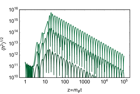
Figure 3: Higgs vacuum fluctuation variance in the $\xi$-resonance scenario. In the lower, middle and upper curves we have used the nonminimal couplings $\xi=10^{1.4}$, $\xi=10^{1.6}$ and $\xi=10^{1.8}$ respectively. Broad resonance occurs strongly for $\xi>10^{1.6}$.

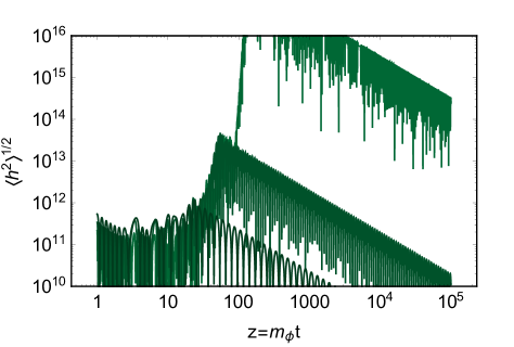
Figure 4: Higgs vacuum fluctuation variance in the $g$-resonance scenario, where we ignore back reaction effects. In the lower, middle and upper curves we have used the inflaton-Higgs coupling $g=10^{-4.4},10^{-4}$ and $10^{-3.6}$ respectively. Broad resonance occurs strongly for $g>10^{-4}$.

IV.1 Parametric resonance via nonminimal gravity-Higgs coupling $\xi$

In this subsection, we solve numerically the Mathieu equation in the case of geometric preheating Bassett and Liberati (1998); Tsujikawa, Maeda, and Torii (1999), where $m_{\rm eff}^{2}$ is dominated by the $\xi R$ term. We call this the $\xi$-resonance scenario. In this case $A_{k}$ and $q$ are given by

$$A_{k}\simeq\frac{k^{2}}{a^{2}m^{2}}+\frac{\Phi^{2}\left(z\right)}{2M_{\rm pl}^{2}}\xi,\quad q\simeq\frac{3\Phi^{2}\left(z\right)}{4M_{\rm pl}^{2}}\left(\xi-\frac{1}{4}\right).$$ (62)

In Fig. 3 we show the evolution of the variance of the Higgs vacuum fluctuations as obtained by numerically solving eq. (57) with $A_{k}$ and $q$ as given above. We take three different values for the nonminimal coupling, namely $\xi=10^{1.4},10^{1.6}$ and $10^{1.8}$. We find that broad resonance can occur strongly for $\xi>10^{1.6}$. We see that the nonminimal coupling $\xi$ is constrained to be $\xi<10^{1.6}$ in order not to produce the Higgs AdS domains via the parametric resonance.

IV.2 Parametric resonance via inflaton-Higgs coupling $g$

In this subsection we solve numerically the Mathieu equation in the standard preheating scenario, where $m_{\rm eff}^{2}$ is dominated by the $g^{2}\phi^{2}$ term. We call this the $g$-resonance scenario. In this case $A_{k}$ and $q$ are given by

$$A_{k}\simeq\frac{k^{2}}{a^{2}m_{\phi}^{2}}+\frac{g^{2}\Phi^{2}\left(z\right)}{2m_{\phi}^{2}},\quad q\simeq\frac{g^{2}\Phi^{2}\left(z\right)}{4m_{\phi}^{2}}.$$ (63)

In Fig. 4 we show the evolution of the variance of the Higgs vacuum fluctuations as obtained by numerically solving (57) with $A_{k}$ and $q$ given as above. For the sake of simplicity, here we have neglected back reaction effects, which we comment further on below. We consider three different values for the inflaton-Higgs coupling, namely $g=10^{-4.4},10^{-4}$ and $10^{-3.6}$. Broad resonance can occur strongly for $g>10^{-4}$. However, $g$ is restricted in order not to give rise to large radiative corrections to the inflaton potential Linde (2008),

$$\Delta V_{\rm inf}\simeq\frac{{g}^{4}}{64{\pi}^{2}}{\phi}^{4}\log{\frac{g^{2}{\phi}^{2}}{m_{\phi}^{2}}}.$$ (64)

Thus, for quadratic chaotic inflation-type models, the inflaton-Higgs coupling is constrained to be $g<10^{-3}$. Because $g$-resonance can occur in the parameter range $10^{-4}<g<10^{-3}$, we find an upper bound on $g$ as $g<10^{-4}$.

In the early stages of parametric resonance, our semiclassical approximation is valid. On the other hand, in the later stages, backreaction effects and effects of scattering among the created particles become important (see, e.g. Ref.Boyanovsky et al. (1996)). In this case, our semiclassical approximation may break down. However, well before the backreaction effects become significant, the generated fluctuations of the Higgs field immediately grow and exceeds the hill of the effective potential due to the parametric resonance. Actually, we can estimate the maximal Higgs fluctuation $\left<{h}^{2}\right>\sim\left<{\phi}^{2}\right>\sim m_{\phi}^{2}/g^{2}$ where backreaction effects terminate the amplification of the Higgs fluctuations. The maximal Higgs fluctuation can be estimated as $\sqrt{\left<{h}^{2}\right>}\sim m_{\phi}/g\sim 10^{17}\ {\rm GeV}$ where $m_{\phi}\simeq 7\times 10^{-6}M_{\rm pl}$ and $g\sim 10^{-4}$ and the generated Higgs fluctuations immediately overcomes the instability scale $\Lambda_{I}$ before the backreaction effects become significant. Therefore, the backreaction effects cannot make a significant contribution to the electroweak vacuum stability.

In Fig. 2, we plot the upper bounds on $H/h_{\rm max}$ as a function of the nonminimal gravity-Higgs coupling $\xi$. We have assumed that the effective mass is $m_{\rm eff}=\sqrt{12\xi}H$. In the left panel, we do not include the constraint on $\xi$ coming from parametric amplification of the Higgs during preheating, as this constraint is model dependent, i.e. it depends on how the inflaton behaves after inflation. On the other hand, in the right panel we have included the constraint on $\xi$ arising from broad resonance during the preheating stages. For simplicity, here we assume the quadratic chaotic inflation model with $V_{\rm inf}\left(\phi\right)=\frac{1}{2}m_{\phi}^{2}\phi^{2}$, which gives us the constraint $\xi<10^{1.6}$.

V Thermal fluctuations during the reheating era

During the reheating stage, most of the inflaton energy is transferred to the thermal energy of elementary particles. The reheating process finishes approximately when $H=\Gamma_{\rm tot}$. Therefore, the reheating temperature can be expressed as

$$T_{\rm reh}=\left(\frac{90}{\pi^{3}g_{*}}\right)^{1/4}\sqrt{M_{\rm pl}\Gamma_{\rm tot}},$$ (65)

where $g_{*}$ is the number of relativistic degrees of freedom.

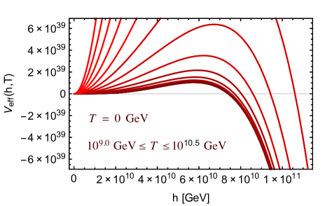
Figure 5: RG improved effective Higgs potential at finite temperature for $T=0\ {\rm GeV}$ and $10^{9.0}\ {\rm GeV}\leq T\leq 10^{10.5}\ {\rm GeV}$ on the present best-fit values of $m_{h}$ and $m_{t}$.

Thermal effects in the reheating can raise the effective potential of the Higgs field. The RG improved effective Higgs potential at finite temperature is given by the familiar zero-temperature corrections and the thermal corrections as

$$V_{\rm eff}\left(h,T\right)=V_{\rm eff}\left(h\right)+\Delta{V}_{\rm eff}\left(h,T\right),$$ (66)

The one-loop thermal corrections to the effective Higgs potential is given as Carrington (1992); Anderson and Hall (1992); Delaunay, Grojean, and Wells (2008),

$$\Delta{V}_{\rm eff}\left(h,T\right) =\sum_{i=W,Z,t}{\frac{{n}_{i}{T}^{4}}{2{\pi}^{2}}\int_{0}^{\infty}{dk{k}^{2}\ln{\left(1\mp{e}^{-\sqrt{{k}^{2}+\frac{{m}_{i}^{2}\left(h\right)}{{T}^{2}}}}\right)}}}$$

$$=\sum_{i=W,Z}{{n}_{i}J_{B}\left(m_{i},T\right)}+\sum_{i=t}{{n}_{i}J_{F}\left(m_{i},T\right)}.$$ (67)

Here we concentrate on the contributions from W bosons, Z bosons and top quarks. $J_{B}$ ($J_{F}$) is the thermal bosonic (fermionic) function, $m_{i}\left(h\right)$ is the background-dependent mass of $W$, $Z$ and $t$.

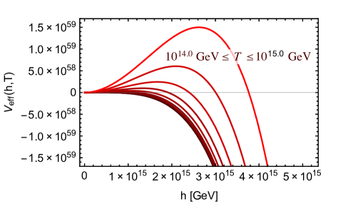
Figure 6: RG improved effective Higgs potential at finite temperature for $10^{14.0}\ {\rm GeV}\leq T\leq 10^{15.0}\ {\rm GeV}$. The maximum of the Higgs potential is $h_{\rm max}=2.62\ T$ for $T=10^{15.0}\ {\rm GeV}$.

In Fig. 5 and Fig. 6, we plot the RG improved effective Higgs potential at finite temperature for a range of temperatures. In Fig. 5, we plot the potential for $T=0\ {\rm GeV}$ and $10^{9.0}\ {\rm GeV}\leq T\leq 10^{10.5}\ {\rm GeV}$. In Fig. 6, we plot the potential for $10^{14.0}\ {\rm GeV}\leq T\leq 10^{15.0}\ {\rm GeV}$. From the figures, we see that although the high-temperature effects raise the effective potential, it cannot be stabilized up to high energy scales unless new physics emerges below the Planck scale. Therefore, if the coherent Higgs field get over $h_{\rm max}$ during inflation or preheating stage, the generated coherent Higgs field cannot go back to the electroweak vacuum by the high temperature effects.

In the high-temperature limit ($T\gg{m}_{i}$), the thermal bosonic (fermionic) function $J_{B}$ ($J_{F}$) can be approximately written as

$$J_{B}\left(m_{i},T\right) \simeq -\frac{\pi^{2}T^{4}}{90}+\frac{m_{i}^{2}T^{2}}{24}-\frac{m_{i}^{3}T}{12\pi}-\frac{{m}_{i}^{4}}{64{\pi}^{2}}\log{\frac{{m}_{i}^{2}}{{a}_{B}{T}^{2}}},$$

$$J_{F}\left(m_{i},T\right) \simeq \frac{7}{8}\frac{\pi^{2}T^{4}}{90}-\frac{m_{i}^{2}T^{2}}{48}-\frac{{m}_{i}^{4}}{64{\pi}^{2}}\log{\frac{{m}_{i}^{2}}{{a}_{F}{T}^{2}}},$$ (68)

where $\log{a_{B}}\simeq 5.408$ and $\log{a_{F}}\simeq 2.635$. Here we omit the terms which are independent of $h$. As such, the one-loop thermal corrections to the effective Higgs potential in the high-temperature limit ($T\gg{m}_{i}$) is approximately written as

$$\Delta{V}_{\rm eff}\left(h,T\right)\simeq\frac{1}{2}c_{T}T^{2}h^{2}+\frac{1}{3}d_{T}Th^{3}+\frac{1}{4}\lambda_{T}h^{4},$$ (69)

where

$$c_{T} = \frac{3g^{2}+g^{\prime 2}+4y_{t}^{2}}{16},\ d_{T}=\frac{6g^{3}+3\left(g^{2}+g^{\prime 2}\right)^{3/2}}{32\pi},$$ (70)

$$\lambda_{T} = \scalebox{0.73}{$\displaystyle\frac{3}{64{\pi}^{2}}\left(-\frac{{g}^{4}}{2}\log{\frac{{m}_{W}^{2}\left(h\right)}{{a}_{B}{T}^{2}}}-\frac{{\left({g}^{2}+{g^{\prime}}^{2}\right)}^{2}}{4}\log{\frac{{m}_{Z}^{2}\left(h\right)}{{a}_{B}{T}^{2}}+4{y}_{t}^{4}}\log{\frac{{m}_{t}^{2}\left(h\right)}{{a}_{F}{T}^{2}}}\right)$}.$$

The variance of the thermal fluctuations of the Higgs is given as Linde (1979, 1992); Dine et al. (1992a, b)

$$\left<{h}^{2}\right>_{T} = \frac{1}{2\pi^{2}}\int_{0}^{\infty}{\frac{{k}^{2}dk}{\sqrt{{k}^{2}+m_{\rm eff}^{2}}\left[e^{\frac{\sqrt{{k}^{2}+m_{\rm eff}^{2}}}{T}}-1\right]}}$$ (71)

$$\simeq \frac{{T}^{2}}{12}-\frac{{m}_{\rm eff}T}{4\pi},$$

where the thermal Higgs mass is $m_{\rm eff}=c_{T}^{1/2}T$ and numerically we obtain $c_{T}\simeq 0.2$.

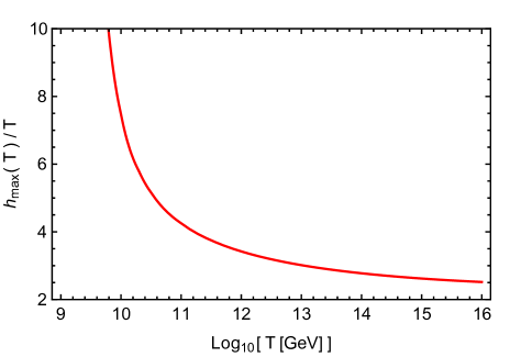
Figure 7: Plot of $h_{\rm max}\left(T\right)/T$ by using RG improved effective Higgs potential at finite temperature.

We can estimate the relation with the thermal Higgs fluctuation and the physical probability of the Higgs AdS domains shown in (37) as

$$\frac{\left<{h}^{2}\right>_{T}}{{h}_{\rm max}^{2}\left({T}\right)}<\frac{1}{6N_{\rm hor}}.$$ (72)

The maximum of the Higgs potential is moved out to larger values of $h$ when thermal corrections are taken into account, and numerically we have found that $h_{\rm max}$ can be well estimated as $h_{\rm max}\left({T}\right)=2\sim 6\ T$. In Fig. 7, we show $h_{\rm max}\left(T\right)/T$ by using the RG improved Higgs potential at the high temperature.

For simplicity, we consider the following condition

$$\frac{6N_{\rm hor}\left<{h}^{2}\right>_{T}}{{h}_{\rm max}^{2}\left({T}\right)}<1.$$ (73)

In Fig. 7, we assume $N_{\rm hor}=60$ and plot $6N_{\rm hor}\left<{h}^{2}\right>_{T}/{h}_{\rm max}^{2}\left({T}\right)$ by using the RG improved effective Higgs potential at the high temperature. When we set $N_{\rm hor}=60$, the constraint (73) gives us the following upper bound on the temperature $T$

$$T<2.4\times 10^{10}{\rm GeV}.$$ (74)

It was previously thought that thermal Higgs fluctuations do not destabilize the standard electroweak vacuum because the probability for the thermal vacuum decay of one Hubble-sized region via the instanton methods is sufficiently small Anderson (1990); Arnold and Vokos (1991); Espinosa and Quiros (1995); Delle Rose, Marzo, and Urbano (2015). However, after inflation, there are the large classical Higgs field and the early Universe contains huge number of independent Hubble-horizon regions. Therefore, the total decay probability due to the thermal Higgs fluctuations would be worse. Although, in this paper, we don’t conclude whether the variance of the thermal Higgs fluctuation destabilize or not, it is necessary to investigate thoroughly the thermal vacuum metastability during the reheating era. We plan to perform a detailed analysis of the stochastic approach and instanton methods in a separate paper. In the rest of this section, we assume that the variance of thermal Higgs fluctuations destabilize the standard electroweak vacuum and show how the Hubble scale $H$ is restricted in this case.

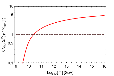
Figure 8: We set $N_{\rm hor}=60$ and plot $6N_{\rm hor}\left<{h}^{2}\right>_{T}/{h}_{\rm max}^{2}\left({T}\right)$ by using the RG improved Higgs potential at the high temperature. We obtain the constraint of the temperature $T<2.4\times 10^{10}{\rm GeV}$.

It is known that the reheating temperature $T_{\rm reh}$ is not the maximal temperature, unless the reheating process is instantaneous. Just after inflation, although still sub-dominant, the decay products from the oscillating inflaton field can become thermalized and produce a so-called dilute plasma. Then, the maximal temperature $T_{\rm max}$ can be estimated by Chung, Kolb, and Riotto (1999); Giudice, Kolb, and Riotto (2001); Kolb, Notari, and Riotto (2003)

$$\scalebox{0.94}{$\displaystyle{T}_{\rm max}=\left(\frac{3}{8}\right)^{2/5}\left(\frac{40}{{\pi}^{2}}\right)^{1/8}\frac{{g}_{*}^{1/8}\left({T}_{\rm reh}\right)}{{g}_{*}^{1/4}\left({T}_{\rm max}\right)}{M}_{\rm pl}^{1/4}H_{\rm end}^{1/4}{T}_{\rm reh}^{1/2}$},$$ (75)

with the reduced Planck mass $M_{\rm pl}=2.4\times 10^{18}\ {\rm GeV}$ and $g_{*}\left({T}\right)$ is the number of relativistic degrees of freedom at the temperature $T$. By using constraints (74) and assuming $T_{\rm reh}<T_{\rm max}$, we can obtain the upper bound on the Hubble scale $H$ as a function of $T_{\rm reh}$.

VI Conclusion

In this paper, we have discussed the stability of the Higgs vacuum during primordial inflation, preheating, and reheating. In the absence of any corrections to the Higgs potential, inflationary vacuum fluctuations of the Higgs field can easily destabilize the standard electroweak vacuum and produce a lot of AdS domains. If a relatively large nonminimal Higgs-gravity coupling or inflaton-Higgs coupling is introduced, a sizable effective mass term is induced, which raises the effective Higgs potential and weakens the Higgs field fluctuations. Therefore, it is possible to suppress the formation of Higgs AdS domains during inflation. However, after inflation, such effective masses are ineffective for stabilizing the large Higgs field. Moreover, nonminimal Higgs-gravity coupling and inflaton-Higgs coupling can also give rise to the generation of large Higgs fluctuations after inflaton via parametric resonance. Hence, such couplings cannot suppress the formation of Higgs AdS domains. We find that the parametric resonance during preheating excludes values of the nonminimal coupling and inflaton-Higgs coupling as $\xi<10^{1.6}$ and $g<10^{-4}$. Furthermore, thermal Higgs fluctuations during the reheating stage cannot be neglected on the electroweak vacuum metastability. Our results show that the thermal Higgs fluctuations produce AdS domains in the reheating stage unless $T<2.4\times 10^{10}{\rm GeV}$. We conclude that through the epochs of inflation, preheating and reheating, a lot of Higgs AdS domains are inevitably produced unless the energy scale of the inflaton potential is much smaller than the GUT scale, or the effective Higgs potential is stabilized below the Planck scale.

Appendix A RG improved effective potential

In this appendix we provide the RG-improved effective potential for the Higgs Ford et al. (1993); Casas, Espinosa, and Quiros (1995); Espinosa and Quiros (1995), which is written in the $\rm\overline{MS}$ scheme and in the ’t Hooft-Landau gauge as

$$V_{\rm eff}\left(h\right)=V_{\rm tree}\left(h\right)+V_{\rm 1-loop}\left(h\right).$$ (76)

The improved tree-level correction to the effective Higgs potential take the form,

$$V_{\rm tree}\left(h\right)=\frac{1}{4}\lambda\left(t\right)h^{4}\left(t\right),$$ (77)

where the running Higgs field is $h\left(t\right)=G\left(t\right)h$. The wavefunction renormalization factor $G\left(t\right)$ is given in terms of the anomalous dimension $\gamma$ as

$$G\left(t\right)=\exp\left(-\int_{0}^{t}{\gamma\left(t^{\prime}\right)dt^{\prime}}\right),$$ (78)

The one-loop correction to the effective Higgs potential at zero-temperature is

$$V_{\rm 1-loop}\left(h\right)=\sum_{i=W,Z,t}{\frac{{n}_{i}}{64{\pi}^{2}}{m}_{i}^{4}\left(h\right)\left[\ln{\frac{{m}_{i}^{2}\left(h\right)}{{\mu}^{2}\left(t\right)}-{C}_{i}}\right]},$$ (79)

where the number of degrees of freedom $n_{i},~{}i=W,Z,t$, and the coefficients $C_{i},~{}i=W,Z,t$ are given by

$$n_{W} = 6,\ n_{Z}=3,\ n_{t}=-12,$$

$$C_{W} = C_{Z}=5/6,\ C_{t}=3/2.$$ (80)

The masses of $W$, $Z$ and $t$ depend on the background Higgs field value $h$ as follows

$$m_{W}^{2}\left(h\right) = \frac{g^{2}\left(t\right)}{4}h^{2}\left(t\right),$$ (81)

$$m_{Z}^{2}\left(h\right) = \frac{g^{2}\left(t\right)+g^{\prime 2}\left(t\right)}{4}h^{2}\left(t\right),$$ (82)

$$m_{t}^{2}\left(h\right) = \frac{y_{t}^{2}\left(t\right)}{2}h^{2}\left(t\right),$$ (83)

where $g$, $g^{\prime}$ and $y_{t}$ are the $SU(2)_{L}$, $U(1)_{Y}$, and top Yukawa couplings, respectively.

We calculate the $\beta$ functions and the anomalous dimension $\gamma$ to two-loop order in the current study. The $\beta$ functions for a generic coupling parameter X are defined through the relation

$$\frac{dX\left(t\right)}{dt}=\sum_{i}{{\beta}_{X}^{\left(i\right)}}.$$ (84)

The $\beta$ functions and anomalous dimension $\gamma$ at one- and two-loop order are given as follows Einhorn and Jones (1992); Machacek and Vaughn (1985, 1984, 1983); Ford, Jack, and Jones (1992); Hertzberg (2012); Holthausen, Lim, and Lindner (2012):

$${\beta}_{\lambda}^{\left(1\right)} = \frac{1}{{\left(4\pi\right)}^{2}}\left[\lambda\left(-9{g}^{2}-3{g^{\prime}}^{2}+12{y}_{t}^{2}\right)+24{\lambda}^{2}+\frac{3}{4}{g}^{4}+\frac{3}{8}{\left({g}^{2}+{g^{\prime}}^{2}\right)}^{2}-6{y}_{t}^{4}\right],$$ (85)

$${\beta}_{{y}_{t}}^{\left(1\right)} = \frac{1}{{\left(4\pi\right)}^{2}}\left[\frac{9}{2}{y}_{t}^{3}+{y}_{t}\left(-\frac{9}{4}{g}^{2}-\frac{17}{12}{g^{\prime}}^{2}-8{g}_{s}^{2}\right)\right],$$ (86)

$${\beta}_{{g}}^{\left(1\right)} = \frac{1}{{\left(4\pi\right)}^{2}}\left[-\frac{19}{6}{g}^{3}\right],\quad{\beta}_{{g^{\prime}}}^{\left(1\right)}=\frac{1}{{\left(4\pi\right)}^{2}}\left[\frac{41}{6}{g^{\prime}}^{3}\right],\quad{\beta}_{{g}_{s}}^{\left(1\right)}=\frac{1}{{\left(4\pi\right)}^{2}}\biggl{[}-7{g}_{s}^{3}\biggl{]},$$ (87)

$${\beta}_{\lambda}^{\left(2\right)} = \frac{1}{{\left(4\pi\right)}^{4}}\biggl{[}-312{\lambda}^{3}-144{\lambda}^{2}{y}_{t}^{2}+36{\lambda}^{2}\left({3g}^{2}+{g^{\prime}}^{2}\right)-3\lambda{y}_{t}^{4}+\lambda{y}_{t}^{2}\left(\frac{45}{2}{g}^{2}+\frac{85}{6}{g^{\prime}}^{2}+80{g}_{s}^{2}\right)$$ (88)

$$-\frac{73}{8}\lambda{g}^{4}+\frac{39}{4}\lambda{g}^{2}{g^{\prime}}^{2}+\frac{629}{24}\lambda{g^{\prime}}^{4}+30{y}_{t}^{6}-32{y}_{t}^{4}{g}_{s}^{2}-\frac{9}{4}{y}_{t}^{2}{g}^{4}-\frac{8}{3}{y}_{t}^{4}{g^{\prime}}^{2}$$

$$+\frac{21}{2}{y}_{t}^{2}{g}^{2}{g^{\prime}}^{2}-\frac{19}{4}{y}_{t}^{2}{g^{\prime}}^{4}+\frac{305}{16}{g}^{6}-\frac{289}{48}{g}^{4}{g^{\prime}}^{2}-\frac{559}{48}{g}^{2}{g^{\prime}}^{4}-\frac{379}{48}{g^{\prime}}^{6}\biggl{]},$$

$${\beta}_{{y}_{t}}^{\left(2\right)} = \frac{1}{{\left(4\pi\right)}^{4}}\biggl{[}{y}_{t}\Bigl{(}-12{y}_{t}^{4}+{y}_{t}^{2}\left(\frac{225}{16}{g}^{2}+\frac{131}{16}{g^{\prime}}^{2}+36{g}_{s}^{2}-12\lambda\right)+\frac{1187}{216}{g^{\prime}}^{4}$$ (89)

$$-\frac{3}{4}{g}^{2}{g^{\prime}}^{2}+\frac{19}{9}{g^{\prime}}^{2}{g}_{s}^{2}-\frac{23}{4}{g}^{4}+9g^{2}{g}_{s}^{2}-108{g}_{s}^{4}+6{\lambda}^{2}\Bigl{)}\biggl{]},$$

$${\beta}_{g}^{\left(2\right)} = \frac{1}{{\left(4\pi\right)}^{4}}\left[{g}^{3}\left(\frac{35}{6}{g}^{2}+\frac{3}{2}{g^{\prime}}^{2}+12{g}_{s}^{2}-\frac{3}{2}{y}_{t}^{2}\right)\right],$$ (90)

$${\beta}_{g^{\prime}}^{\left(2\right)} = \frac{1}{{\left(4\pi\right)}^{4}}\left[{g^{\prime}}^{3}\left(\frac{9}{2}{g}^{2}+\frac{199}{18}{g^{\prime}}^{2}+\frac{44}{3}{g}_{s}^{2}-\frac{17}{6}{y}_{t}^{2}\right)\right],$$ (91)

$${\beta}_{{g}_{s}}^{\left(2\right)} = \frac{1}{{\left(4\pi\right)}^{4}}\left[{{g}_{s}}^{3}\left(\frac{9}{2}{g}^{2}+\frac{11}{6}{g^{\prime}}^{2}-26{g}_{s}^{2}-2{y}_{t}^{2}\right)\right],$$ (92)

$${\gamma}^{\left(1\right)} = \frac{1}{{\left(4\pi\right)}^{2}}\left[3{y}_{t}^{2}-\frac{9{g}^{2}}{4}-\frac{3{g^{\prime}}^{2}}{4}\right],$$ (93)

$${\gamma}^{\left(2\right)} = \frac{1}{{\left(4\pi\right)}^{4}}\left[6{\lambda}^{2}-\frac{27}{4}{y}_{t}^{4}+\frac{5}{2}\left(\frac{9}{4}{g}^{2}+\frac{17}{12}{g^{\prime}}^{2}+8{g}_{s}^{2}\right){y}_{t}^{2}-\frac{271}{32}{g}^{4}+\frac{9}{16}{g}^{2}{g^{\prime}}^{2}+\frac{431}{96}{g^{\prime}}^{4}\right].$$ (94)

References

- Aad et al. (2015) G. Aad et al. (ATLAS, CMS), Proceedings, Meeting of the APS Division of Particles and Fields (DPF 2015), Phys. Rev. Lett. 114, 191803 (2015), arXiv:1503.07589 [hep-ex] .
- Aad et al. (2013) G. Aad et al. (ATLAS), Phys.Lett. B726, 88 (2013), arXiv:1307.1427 [hep-ex] .
- Chatrchyan et al. (2014) S. Chatrchyan et al. (CMS), Phys.Rev. D89, 092007 (2014), arXiv:1312.5353 [hep-ex] .
- Giardino et al. (2014) P. P. Giardino, K. Kannike, I. Masina, M. Raidal, and A. Strumia, JHEP 1405, 046 (2014), arXiv:1303.3570 [hep-ph] .
- ATLAS et al. (2014) T. ATLAS, CDF, CMS, and D0 Collaborations, ArXiv e-prints (2014), arXiv:1403.4427 [hep-ex] .
- Buttazzo et al. (2013) D. Buttazzo, G. Degrassi, P. P. Giardino, G. F. Giudice, F. Sala, et al., JHEP 1312, 089 (2013), arXiv:1307.3536 [hep-ph] .
- Kobzarev, Okun, and Voloshin (1975) I. Yu. Kobzarev, L. B. Okun, and M. B. Voloshin, Sov. J. Nucl. Phys. 20, 644 (1975), [Yad. Fiz.20,1229(1974)].
- Coleman (1977) S. R. Coleman, Phys. Rev. D15, 2929 (1977), [Erratum: Phys. Rev.D16,1248(1977)].
- Callan and Coleman (1977) C. G. Callan, Jr. and S. R. Coleman, Phys. Rev. D16, 1762 (1977).
- Degrassi et al. (2012) G. Degrassi, S. Di Vita, J. Elias-Miro, J. R. Espinosa, G. F. Giudice, et al., JHEP 1208, 098 (2012), arXiv:1205.6497 [hep-ph] .
- Isidori, Ridolfi, and Strumia (2001) G. Isidori, G. Ridolfi, and A. Strumia, Nucl.Phys. B609, 387 (2001), arXiv:hep-ph/0104016 [hep-ph] .
- Ellis et al. (2009) J. Ellis, J. Espinosa, G. Giudice, A. Hoecker, and A. Riotto, Phys.Lett. B679, 369 (2009), arXiv:0906.0954 [hep-ph] .
- Elias-Miro et al. (2012) J. Elias-Miro, J. R. Espinosa, G. F. Giudice, G. Isidori, A. Riotto, et al., Phys.Lett. B709, 222 (2012), arXiv:1112.3022 [hep-ph] .
- Espinosa, Giudice, and Riotto (2008) J. Espinosa, G. Giudice, and A. Riotto, JCAP 0805, 002 (2008), arXiv:0710.2484 [hep-ph] .
- Fairbairn and Hogan (2014) M. Fairbairn and R. Hogan, Phys.Rev.Lett. 112, 201801 (2014), arXiv:1403.6786 [hep-ph] .
- Kobakhidze and Spencer-Smith (2013) A. Kobakhidze and A. Spencer-Smith, Phys.Lett. B722, 130 (2013), arXiv:1301.2846 [hep-ph] .
- Lebedev and Westphal (2013) O. Lebedev and A. Westphal, Phys.Lett. B719, 415 (2013), arXiv:1210.6987 [hep-ph] .
- Enqvist, Meriniemi, and Nurmi (2013) K. Enqvist, T. Meriniemi, and S. Nurmi, JCAP 1310, 057 (2013), arXiv:1306.4511 [hep-ph] .
- Herranen et al. (2014) M. Herranen, T. Markkanen, S. Nurmi, and A. Rajantie, Phys.Rev.Lett. 113, 211102 (2014), arXiv:1407.3141 [hep-ph] .
- Kobakhidze and Spencer-Smith (2014) A. Kobakhidze and A. Spencer-Smith, (2014), arXiv:1404.4709 [hep-ph] .
- Kamada (2015) K. Kamada, Phys. Lett. B742, 126 (2015), arXiv:1409.5078 [hep-ph] .
- Enqvist, Meriniemi, and Nurmi (2014) K. Enqvist, T. Meriniemi, and S. Nurmi, JCAP 1407, 025 (2014), arXiv:1404.3699 [hep-ph] .
- Hook et al. (2015) A. Hook, J. Kearney, B. Shakya, and K. M. Zurek, JHEP 1501, 061 (2015), arXiv:1404.5953 [hep-ph] .
- Kearney, Yoo, and Zurek (2015) J. Kearney, H. Yoo, and K. M. Zurek, (2015), arXiv:1503.05193 [hep-th] .
- Espinosa et al. (2015) J. R. Espinosa, G. F. Giudice, E. Morgante, A. Riotto, L. Senatore, et al., (2015), arXiv:1505.04825 [hep-ph] .
- Gross, Lebedev, and Zatta (2015) C. Gross, O. Lebedev, and M. Zatta, (2015), arXiv:1506.05106 [hep-ph] .
- Herranen et al. (2015) M. Herranen, T. Markkanen, S. Nurmi, and A. Rajantie, (2015), arXiv:1506.04065 [hep-ph] .
- Ema, Mukaida, and Nakayama (2016) Y. Ema, K. Mukaida, and K. Nakayama, (2016), arXiv:1602.00483 [hep-ph] .
- Di Luzio and Mihaila (2014) L. Di Luzio and L. Mihaila, JHEP 1406, 079 (2014), arXiv:1404.7450 [hep-ph] .
- Andreassen, Frost, and Schwartz (2015) A. Andreassen, W. Frost, and M. D. Schwartz, Phys.Rev. D91, 016009 (2015), arXiv:1408.0287 [hep-ph] .
- Andreassen, Frost, and Schwartz (2014) A. Andreassen, W. Frost, and M. D. Schwartz, Phys.Rev.Lett. 113, 241801 (2014), arXiv:1408.0292 [hep-ph] .
- Coleman and De Luccia (1980) S. R. Coleman and F. De Luccia, Phys.Rev. D21, 3305 (1980).
- Hawking and Moss (1982) S. Hawking and I. Moss, Phys.Lett. B110, 35 (1982).
- Linde (1992) A. D. Linde, Nucl.Phys. B372, 421 (1992), arXiv:hep-th/9110037 [hep-th] .
- Nambu (1989) Y. Nambu, Prog.Theor.Phys. 81, 1037 (1989).
- Nambu and Sasaki (1989) Y. Nambu and M. Sasaki, Phys.Lett. B219, 240 (1989).
- Sekino, Shenker, and Susskind (2010) Y. Sekino, S. Shenker, and L. Susskind, Phys.Rev. D81, 123515 (2010), arXiv:1003.1347 [hep-th] .
- Birrell and Davies (1984) N. D. Birrell and P. C. W. Davies, Quantum Fields in Curved Space, Cambridge Monographs on Mathematical Physics (Cambridge Univ. Press, Cambridge, UK, 1984).
- Kofman, Linde, and Starobinsky (1997) L. Kofman, A. D. Linde, and A. A. Starobinsky, Phys. Rev. D56, 3258 (1997), arXiv:hep-ph/9704452 [hep-ph] .
- Kofman, Linde, and Starobinsky (1996) L. Kofman, A. D. Linde, and A. A. Starobinsky, Phys. Rev. Lett. 76, 1011 (1996), arXiv:hep-th/9510119 [hep-th] .
- Jin and Tsujikawa (2006) Y. Jin and S. Tsujikawa, Class. Quant. Grav. 23, 353 (2006), arXiv:hep-ph/0411164 [hep-ph] .
- Liddle et al. (2000) A. R. Liddle, D. H. Lyth, K. A. Malik, and D. Wands, Phys. Rev. D61, 103509 (2000), arXiv:hep-ph/9912473 [hep-ph] .
- Bassett and Liberati (1998) B. A. Bassett and S. Liberati, Phys. Rev. D58, 021302 (1998), [Erratum: Phys. Rev.D60,049902(1999)], arXiv:hep-ph/9709417 [hep-ph] .
- Tsujikawa, Maeda, and Torii (1999) S. Tsujikawa, K.-i. Maeda, and T. Torii, Phys. Rev. D60, 063515 (1999), arXiv:hep-ph/9901306 [hep-ph] .
- Linde (2008) A. D. Linde, 22nd IAP Colloquium on Inflation + 25: The First 25 Years of Inflationary Cosmology Paris, France, June 26-30, 2006, Lect. Notes Phys. 738, 1 (2008), arXiv:0705.0164 [hep-th] .
- Boyanovsky et al. (1996) D. Boyanovsky, H. J. de Vega, R. Holman, and J. F. J. Salgado, Phys. Rev. D54, 7570 (1996), arXiv:hep-ph/9608205 [hep-ph] .
- Carrington (1992) M. Carrington, Phys.Rev. D45, 2933 (1992).
- Anderson and Hall (1992) G. W. Anderson and L. J. Hall, Phys.Rev. D45, 2685 (1992).
- Delaunay, Grojean, and Wells (2008) C. Delaunay, C. Grojean, and J. D. Wells, JHEP 0804, 029 (2008), arXiv:0711.2511 [hep-ph] .
- Linde (1979) A. D. Linde, Rept. Prog. Phys. 42, 389 (1979).
- Dine et al. (1992a) M. Dine, R. G. Leigh, P. Y. Huet, A. D. Linde, and D. A. Linde, Phys. Rev. D46, 550 (1992a), arXiv:hep-ph/9203203 [hep-ph] .
- Dine et al. (1992b) M. Dine, R. G. Leigh, P. Huet, A. D. Linde, and D. A. Linde, Phys. Lett. B283, 319 (1992b), arXiv:hep-ph/9203201 [hep-ph] .
- Anderson (1990) G. W. Anderson, Phys. Lett. B243, 265 (1990).
- Arnold and Vokos (1991) P. B. Arnold and S. Vokos, Phys. Rev. D44, 3620 (1991).
- Espinosa and Quiros (1995) J. R. Espinosa and M. Quiros, Phys. Lett. B353, 257 (1995), arXiv:hep-ph/9504241 [hep-ph] .
- Delle Rose, Marzo, and Urbano (2015) L. Delle Rose, C. Marzo, and A. Urbano, (2015), arXiv:1507.06912 [hep-ph] .
- Chung, Kolb, and Riotto (1999) D. J. Chung, E. W. Kolb, and A. Riotto, Phys.Rev. D60, 063504 (1999), arXiv:hep-ph/9809453 [hep-ph] .
- Giudice, Kolb, and Riotto (2001) G. F. Giudice, E. W. Kolb, and A. Riotto, Phys.Rev. D64, 023508 (2001), arXiv:hep-ph/0005123 [hep-ph] .
- Kolb, Notari, and Riotto (2003) E. W. Kolb, A. Notari, and A. Riotto, Phys.Rev. D68, 123505 (2003), arXiv:hep-ph/0307241 [hep-ph] .
- Ford et al. (1993) C. Ford, D. R. T. Jones, P. W. Stephenson, and M. B. Einhorn, Nucl. Phys. B395, 17 (1993), arXiv:hep-lat/9210033 [hep-lat] .
- Casas, Espinosa, and Quiros (1995) J. A. Casas, J. R. Espinosa, and M. Quiros, Phys. Lett. B342, 171 (1995), arXiv:hep-ph/9409458 [hep-ph] .
- Einhorn and Jones (1992) M. B. Einhorn and D. R. T. Jones, Phys. Rev. D 46, 5206 (1992).
- Machacek and Vaughn (1985) M. E. Machacek and M. T. Vaughn, Nuclear Physics B 249, 70 (1985).
- Machacek and Vaughn (1984) M. E. Machacek and M. T. Vaughn, Nuclear Physics B 236, 221 (1984).
- Machacek and Vaughn (1983) M. E. Machacek and M. T. Vaughn, Nuclear Physics B 222, 83 (1983).
- Ford, Jack, and Jones (1992) C. Ford, I. Jack, and D. R. T. Jones, Nucl. Phys. B387, 373 (1992), [Erratum: Nucl. Phys.B504,551(1997)], arXiv:hep-ph/0111190 [hep-ph] .
- Hertzberg (2012) M. P. Hertzberg, (2012), arXiv:1210.3624 [hep-ph] .
- Holthausen, Lim, and Lindner (2012) M. Holthausen, K. S. Lim, and M. Lindner, JHEP 02, 037 (2012), arXiv:1112.2415 [hep-ph] .