From Softmax to Sparsemax:
A Sparse Model of Attention and Multi-Label Classification
André F. T. Martins†♯ andre.martins@unbabel.com
Ramón F. Astudillo†⋄ ramon@unbabel.com
†Unbabel Lda, Rua Visconde de Santarém, 67-B, 1000-286 Lisboa, Portugal
♯Instituto de Telecomunicações (IT), Instituto Superior Técnico, Av. Rovisco Pais, 1, 1049-001 Lisboa, Portugal
⋄Instituto de Engenharia de Sistemas e Computadores (INESC-ID), Rua Alves Redol, 9, 1000-029 Lisboa, Portugal
Abstract
We propose sparsemax, a new activation function similar to the traditional softmax, but able to output sparse probabilities. After deriving its properties, we show how its Jacobian can be efficiently computed, enabling its use in a network trained with backpropagation. Then, we propose a new smooth and convex loss function which is the sparsemax analogue of the logistic loss. We reveal an unexpected connection between this new loss and the Huber classification loss. We obtain promising empirical results in multi-label classification problems and in attention-based neural networks for natural language inference. For the latter, we achieve a similar performance as the traditional softmax, but with a selective, more compact, attention focus.
1 Introduction
The softmax transformation is a key component of several statistical learning models, encompassing multinomial logistic regression (McCullagh & Nelder, 1989), action selection in reinforcement learning (Sutton & Barto, 1998), and neural networks for multi-class classification (Bridle, 1990; Goodfellow et al., 2016). Recently, it has also been used to design attention mechanisms in neural networks, with important achievements in machine translation (Bahdanau et al., 2015), image caption generation (Xu et al., 2015), speech recognition (Chorowski et al., 2015), memory networks (Sukhbaatar et al., 2015), and various tasks in natural language understanding (Hermann et al., 2015; Rocktäschel et al., 2015; Rush et al., 2015) and computation learning (Graves et al., 2014; Grefenstette et al., 2015).
There are a number of reasons why the softmax transformation is so appealing. It is simple to evaluate and differentiate, and it can be turned into the (convex) negative log-likelihood loss function by taking the logarithm of its output. Alternatives proposed in the literature, such as the Bradley-Terry model (Bradley & Terry, 1952; Zadrozny, 2001; Menke & Martinez, 2008), the multinomial probit (Albert & Chib, 1993), the spherical softmax (Ollivier, 2013; Vincent, 2015; de Brébisson & Vincent, 2015), or softmax approximations (Bouchard, 2007), while theoretically or computationally advantageous for certain scenarios, lack some of the convenient properties of softmax.
In this paper, we propose the sparsemax transformation. Sparsemax has the distinctive feature that it can return sparse posterior distributions, that is, it may assign exactly zero probability to some of its output variables. This property makes it appealing to be used as a filter for large output spaces, to predict multiple labels, or as a component to identify which of a group of variables are potentially relevant for a decision, making the model more interpretable. Crucially, this is done while preserving most of the attractive properties of softmax: we show that sparsemax is also simple to evaluate, it is even cheaper to differentiate, and that it can be turned into a convex loss function.
To sum up, our contributions are as follows:
- •
-
•
We derive the Jacobian of sparsemax, comparing it to the softmax case, and show that it can lead to faster gradient backpropagation (§2.5).
-
•
We propose the sparsemax loss, a new loss function that is the sparsemax analogue of logistic regression (§3). We show that it is convex, everywhere differentiable, and can be regarded as a multi-class generalization of the Huber classification loss, an important tool in robust statistics (Huber, 1964; Zhang, 2004).
- •
-
•
Finally, we devise a neural selective attention mechanism using the sparsemax transformation, evaluating its performance on a natural language inference problem, with encouraging results (§4.3).
2 The Sparsemax Transformation
2.1 Definition
Let be the -dimensional simplex. We are interested in functions that map vectors in to probability distributions in . Such functions are useful for converting a vector of real weights (e.g., label scores) to a probability distribution (e.g. posterior probabilities of labels). The classical example is the softmax function, defined componentwise as:
| (1) |
A limitation of the softmax transformation is that the resulting probability distribution always has full support, i.e., for every and . This is a disadvantage in applications where a sparse probability distribution is desired, in which case it is common to define a threshold below which small probability values are truncated to zero.
In this paper, we propose as an alternative the following transformation, which we call sparsemax:
| (2) |
In words, sparsemax returns the Euclidean projection of the input vector onto the probability simplex. This projection is likely to hit the boundary of the simplex, in which case becomes sparse. We will see that sparsemax retains most of the important properties of softmax, having in addition the ability of producing sparse distributions.
2.2 Closed-Form Solution
Projecting onto the simplex is a well studied problem, for which linear-time algorithms are available (Michelot, 1986; Pardalos & Kovoor, 1990; Duchi et al., 2008). We start by recalling the well-known result that such projections correspond to a soft-thresholding operation. Below, we use the notation and .
Proposition 1
The solution of Eq. 2 is of the form:
| (3) |
where is the (unique) function that satisfies for every . Furthermore, can be expressed as follows. Let be the sorted coordinates of , and define . Then,
| (4) |
where is the support of .
Proof: See App. A.1 in the supplemental material.
In essence, Prop. 1 states that all we need for evaluating the sparsemax transformation is to compute the threshold ; all coordinates above this threshold (the ones in the set ) will be shifted by this amount, and the others will be truncated to zero. We call in Eq. 4 the threshold function. This piecewise linear function will play an important role in the sequel. Alg. 1 illustrates a naïve algorithm that uses Prop. 1 for evaluating the sparsemax.111More elaborate algorithms exist based on linear-time selection (Blum et al., 1973; Pardalos & Kovoor, 1990).
2.3 Basic Properties
We now highlight some properties that are common to softmax and sparsemax. Let , and denote by the set of maximal components of . We define the indicator vector , whose th component is if , and otherwise. We further denote by the gap between the maximal components of and the second largest. We let and be vectors of zeros and ones, respectively.
Proposition 2
The following properties hold for .
-
1.
and (uniform distribution, and distribution peaked on the maximal components of , respectively). For sparsemax, the last equality holds for any .
-
2.
, for any (i.e., is invariant to adding a constant to each coordinate).
-
3.
for any permutation matrix (i.e., commutes with permutations).
-
4.
If , then , where for softmax, and for sparsemax.
Proof: See App. A.2 in the supplemental material.
Interpreting as a “temperature parameter,” the first part of Prop. 2 shows that the sparsemax has the same “zero-temperature limit” behaviour as the softmax, but without the need of making the temperature arbitrarily small.
Prop. 2 is reassuring, since it shows that the sparsemax transformation, despite being defined very differently from the softmax, has a similar behaviour and preserves the same invariances. Note that some of these properties are not satisfied by other proposed replacements of the softmax: for example, the spherical softmax (Ollivier, 2013), defined as , does not satisfy properties 2 and 4.
2.4 Two and Three-Dimensional Cases
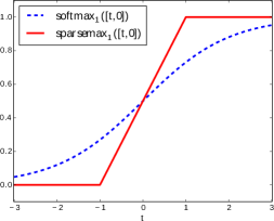
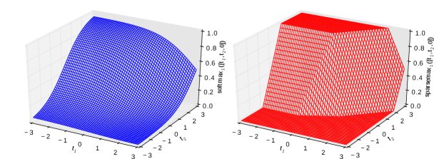
For the two-class case, it is well known that the softmax activation becomes the logistic (sigmoid) function. More precisely, if , then . We next show that the analogous in sparsemax is the “hard” version of the sigmoid. In fact, using Prop. 1, Eq. 4, we have that, for ,
| (5) |
and therefore
| (6) |
Fig. 1 provides an illustration for the two and three-dimensional cases. For the latter, we parameterize and plot and as a function of and . We can see that sparsemax is piecewise linear, but asymptotically similar to the softmax.
2.5 Jacobian of Sparsemax
The Jacobian matrix of a transformation , , is of key importance to train models with gradient-based optimization. We next derive the Jacobian of the sparsemax activation, but before doing so, let us recall how the Jacobian of the softmax looks like. We have
| (7) | |||||
where is the Kronecker delta, which evaluates to if and otherwise. Letting , the full Jacobian can be written in matrix notation as
| (8) |
where is a matrix with in the main diagonal.
Let us now turn to the sparsemax case. The first thing to note is that sparsemax is differentiable everywhere except at splitting points where the support set changes, i.e., where for some and infinitesimal .222For those points, we can take an arbitrary matrix in the set of generalized Clarke’s Jacobians (Clarke, 1983), the convex hull of all points of the form , where . From Eq. 3, we have that:
| (9) |
It remains to compute the gradient of the threshold function . From Eq. 4, we have:
| (10) |
Note that . Therefore we obtain:
| (11) |
Let be an indicator vector whose th entry is if , and otherwise. We can write the Jacobian matrix as
| (12) |
It is instructive to compare Eqs. 8 and 12. We may regard the Jacobian of sparsemax as the Laplacian of a graph whose elements of are fully connected. To compute it, we only need , which can be obtained in time with the same algorithm that evaluates the sparsemax.
Often, e.g., in the gradient backpropagation algorithm, it is not necessary to compute the full Jacobian matrix, but only the product between the Jacobian and a given vector . In the softmax case, from Eq. 8, we have:
| (13) |
where denotes the Hadamard product; this requires a linear-time computation. For the sparsemax case, we have:
| (14) |
Interestingly, if has already been evaluated (i.e., in the forward step), then so has , hence the nonzeros of can be computed in only time, which can be sublinear. This can be an important advantage of sparsemax over softmax if is large.
3 A Loss Function for Sparsemax
Now that we have defined the sparsemax transformation and established its main properties, we show how to use this transformation to design a new loss function that resembles the logistic loss, but can yield sparse posterior distributions. Later (in §4.1–4.2), we apply this loss to label proportion estimation and multi-label classification.
3.1 Logistic Loss
Consider a dataset , where each is an input vector and each is a target output label. We consider regularized empirical risk minimization problems of the form
| (15) |
where is a loss function, is a matrix of weights, and is a bias vector. The loss function associated with the softmax is the logistic loss (or negative log-likelihood):
| (16) | |||||
where , and is the “gold” label. The gradient of this loss is, invoking Eq. 7,
| (17) |
where denotes the delta distribution on , if , and otherwise. This is a well-known result; when plugged into a gradient-based optimizer, it leads to updates that move probability mass from the distribution predicted by the current model (i.e., ) to the gold label (via ). Can we have something similar for sparsemax?
3.2 Sparsemax Loss
A nice aspect of the log-likelihood (Eq. 16) is that adding up loss terms for several examples, assumed i.i.d, we obtain the log-probability of the full training data. Unfortunately, this idea cannot be carried out to sparsemax: now, some labels may have exactly probability zero, so any model that assigns zero probability to a gold label would zero out the probability of the entire training sample. This is of course highly undesirable. One possible workaround is to define
| (18) |
where is a small constant, and is a “perturbed” sparsemax. However, this loss is non-convex, unlike the one in Eq. 16.
Another possibility, which we explore here, is to construct an alternative loss function whose gradient resembles the one in Eq. 17. Note that the gradient is particularly important, since it is directly involved in the model updates for typical optimization algorithms. Formally, we want to be a differentiable function such that
| (19) |
We show below that this property is fulfilled by the following function, henceforth called the sparsemax loss:
| (20) |
where is the square of the threshold function in Eq. 4. This loss, which has never been considered in the literature to the best of our knowledge, has a number of interesting properties, stated in the next proposition.
Proposition 3
The following holds:
-
1.
is differentiable everywhere, and its gradient is given by the expression in Eq. 19.
-
2.
is convex.
-
3.
, .
-
4.
, for all and .
-
5.
The following statements are all equivalent: (i) ; (ii) ; (iii) margin separation holds, .
Proof: See App. A.3 in the supplemental material.
Note that the first four properties in Prop. 3 are also satisfied by the logistic loss, except that the gradient is given by Eq. 17. The fifth property is particularly interesting, since it is satisfied by the hinge loss of support vector machines. However, unlike the hinge loss, is everywhere differentiable, hence amenable to smooth optimization methods such as L-BFGS or accelerated gradient descent (Liu & Nocedal, 1989; Nesterov, 1983).
3.3 Relation to the Huber Loss
Coincidentally, as we next show, the sparsemax loss in the binary case reduces to the Huber classification loss, an important loss function in robust statistics (Huber, 1964).
Let us note first that, from Eq. 20, we have, if ,
| (21) |
and, if ,
| (22) |
where are the sorted components of . Note that the second expression, when , equals the first one, which asserts the continuity of the loss even though is non-continuous on .
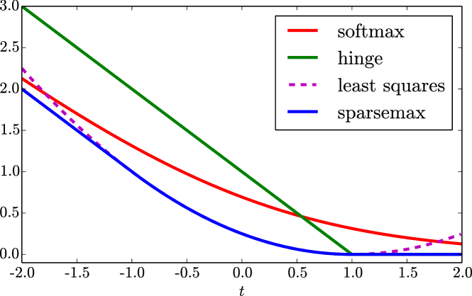
In the two-class case, we have if (unit margin separation), and otherwise. Assume without loss of generality that the correct label is , and define . From Eqs. 21–22, we have
| (23) |
whose graph is shown in Fig. 2. This loss is a variant of the Huber loss adapted for classification, and has been called “modified Huber loss” by Zhang (2004); Zou et al. (2006).
3.4 Generalization to Multi-Label Classification
We end this section by showing a generalization of the loss functions in Eqs. 16 and 20 to multi-label classification, i.e., problems in which the target is a non-empty set of labels rather than a single label.333Not to be confused with “multi-class classification,” which denotes problems where and . Such problems have attracted recent interest (Zhang & Zhou, 2014).
More generally, we consider the problem of estimating sparse label proportions, where the target is a probability distribution , such that . We assume a training dataset , where each is an input vector and each is a target distribution over outputs, assumed sparse.444This scenario is also relevant for “learning with a probabilistic teacher” (Agrawala, 1970) and semi-supervised learning (Chapelle et al., 2006), as it can model label uncertainty. This subsumes single-label classification, where all are delta distributions concentrated on a single class. The generalization of the multinomial logistic loss to this setting is
where and denote the Kullback-Leibler divergence and the Shannon entropy, respectively. Note that, up to a constant, this loss is equivalent to standard logistic regression with soft labels. The gradient of this loss is
| (25) |
The corresponding generalization in the sparsemax case is:
| (26) |
which satisfies the properties in Prop. 3 and has gradient
| (27) |
4 Experiments
We next evaluate empirically the ability of sparsemax for addressing two classes of problems:
- 1.
- 2.
4.1 Label Proportion Estimation
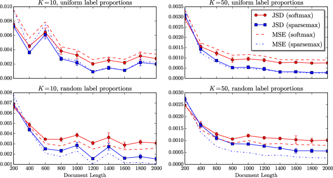
We show simulation results for sparse label proportion estimation on synthetic data. Since sparsemax can predict sparse distributions, we expect its superiority in this task. We generated datasets with 1,200 training and 1,000 test examples. Each example emulates a “multi-labeled document”: a variable-length sequence of word symbols, assigned to multiple topics (labels). We pick the number of labels by sampling from a Poisson distribution with rejection sampling, and draw the labels from a multinomial. Then, we pick a document length from a Poisson, and repeatedly sample its words from the mixture of the label-specific multinomials. We experimented with two settings: uniform mixtures ( for the active labels ) and random mixtures (whose label proportions were drawn from a flat Dirichlet).555Note that, with uniform mixtures, the problem becomes essentially multi-label classification. We set the vocabulary size to be equal to the number of labels , and varied the average document length between 200 and 2,000 words. We trained models by optimizing Eq. 3.1 with (Eqs. 3.4 and 26). We picked the regularization constant with 5-fold cross-validation.
Results are shown in Fig. 3. We report the mean squared error (average of on the test set, where and are respectively the target and predicted label posteriors) and the Jensen-Shannon divergence (average of ).666Note that the KL divergence is not an appropriate metric here, since the sparsity of and could lead to values. We observe that the two losses perform similarly for small document lengths (where the signal is weaker), but as the average document length exceeds 400, the sparsemax loss starts outperforming the logistic loss consistently. This is because with a stronger signal the sparsemax estimator manages to identify correctly the support of the label proportions , contributing to reduce both the mean squared error and the JS divergence. This occurs both for uniform and random mixtures.
4.2 Multi-Label Classification on Benchmark Datasets
Next, we ran experiments in five benchmark multi-label classification datasets: the four small-scale datasets used by Koyejo et al. (2015),777Obtained from http://mulan.sourceforge.net/datasets-mlc.html. and the much larger Reuters RCV1 v2 dataset of Lewis et al. (2004).888Obtained from https://www.csie.ntu.edu.tw/~cjlin/libsvmtools/datasets/multilabel.html. For all datasets, we removed examples without labels (i.e. where ). For all but the Reuters dataset, we normalized the features to have zero mean and unit variance. Statistics for these datasets are presented in Table 1.
| Dataset | Descr. | #labels | #train | #test |
| Scene | images | 6 | 1211 | 1196 |
| Emotions | music | 6 | 393 | 202 |
| Birds | audio | 19 | 323 | 322 |
| CAL500 | music | 174 | 400 | 100 |
| Reuters | text | 103 | 23,149 | 781,265 |
| Dataset | Logistic | Softmax | Sparsemax |
|---|---|---|---|
| Scene | 70.96 / 72.95 | 74.01 / 75.03 | 73.45 / 74.57 |
| Emotions | 66.75 / 68.56 | 67.34 / 67.51 | 66.38 / 66.07 |
| Birds | 45.78 / 33.77 | 48.67 / 37.06 | 49.44 / 39.13 |
| CAL500 | 48.88 / 24.49 | 47.46 / 23.51 | 48.47 / 26.20 |
| Reuters | 81.19 / 60.02 | 79.47 / 56.30 | 80.00 / 61.27 |
Recent work has investigated the consistency of multi-label classifiers for various micro and macro-averaged metrics (Gao & Zhou, 2013; Koyejo et al., 2015), among which a plug-in classifier that trains independent binary logistic regressors on each label, and then tunes a probability threshold on validation data. At test time, those labels whose posteriors are above the threshold are predicted to be “on.” We used this procedure (called Logistic) as a baseline for comparison. Our second baseline (Softmax) is a multinomial logistic regressor, using the loss function in Eq. 3.4, where the target distribution is set to uniform over the active labels. A similar probability threshold is used for prediction, above which a label is predicted to be “on.” We compare these two systems with the sparsemax loss function of Eq. 26. We found it beneficial to scale the label scores by a constant at test time, before applying the sparsemax transformation, to make the resulting distribution more sparse. We then predict the th label to be “on” if .
We optimized the three losses with L-BFGS (for a maximum of 100 epochs), tuning the hyperparameters in a held-out validation set (for the Reuters dataset) and with 5-fold cross-validation (for the other four datasets). The hyperparameters are the regularization constant , the probability thresholds for Logistic and for Softmax, and the coefficient for Sparsemax.
Results are shown in Table 2. Overall, the performances of the three losses are all very similar, with a slight advantage of Sparsemax, which attained the highest results in 4 out of 10 experiments, while Logistic and Softmax won 3 times each. In particular, sparsemax appears better suited for problems with larger numbers of labels.
4.3 Neural Networks with Attention Mechanisms
We now assess the suitability of the sparsemax transformation to construct a “sparse” neural attention mechanism.
We ran experiments on the task of natural language inference, using the recently released SNLI 1.0 corpus (Bowman et al., 2015), a collection of 570,000 human-written English sentence pairs. Each pair consists of a premise and an hypothesis, manually labeled with one the labels entailment, contradiction, or neutral. We used the provided training, development, and test splits.
The architecture of our system, shown in Fig. 4, is the same as the one proposed by Rocktäschel et al. (2015). We compare the performance of four systems: NoAttention, a (gated) RNN-based system similar to Bowman et al. (2015); LogisticAttention, an attention-based system with independent logistic activations; SoftAttention, a near-reproduction of the Rocktäschel et al. (2015)’s attention-based system; and SparseAttention, which replaces the latter softmax-activated attention mechanism by a sparsemax activation.
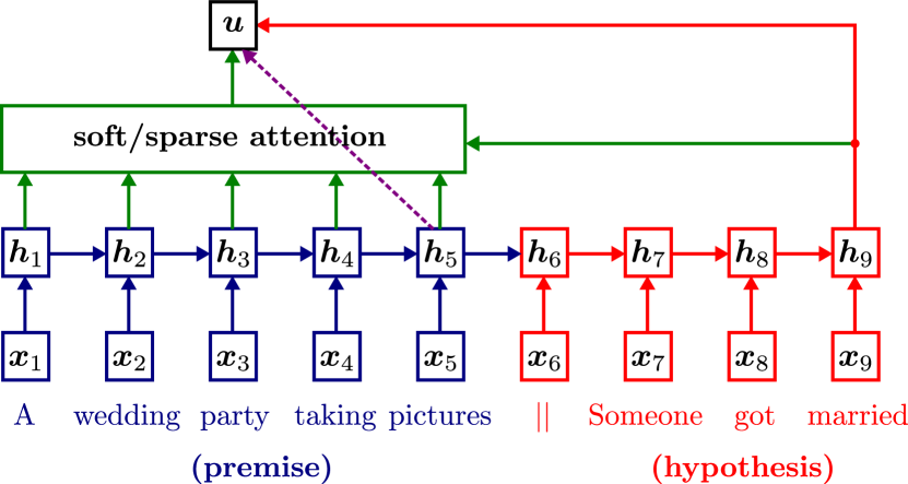
We represent the words in the premise and in the hypothesis with 300-dimensional GloVe vectors (Pennington et al., 2014), not optimized during training, which we linearly project onto a -dimensional subspace (Astudillo et al., 2015).999We used GloVe-840B embeddings trained on Common Crawl (http://nlp.stanford.edu/projects/glove/). We denote by and , respectively, the projected premise and hypothesis word vectors. These sequences are then fed into two recurrent networks (one for each). Instead of long short-term memories, as Rocktäschel et al. (2015), we used gated recurrent units (GRUs, Cho et al. 2014), which behave similarly but have fewer parameters. Our premise GRU generates a state sequence as follows:
| (28) | |||||
| (29) | |||||
| (30) | |||||
| (31) |
with model parameters and . Likewise, our hypothesis GRU (with distinct parameters) generates a state sequence , being initialized with the last state from the premise (). The NoAttention system then computes the final state based on the last states from the premise and the hypothesis as follows:
| (32) |
where and . Finally, it predicts a label from with a standard softmax layer. The SoftAttention system, instead of using the last premise state , computes a weighted average of premise words with an attention mechanism, replacing Eq. 32 by
| (33) | |||||
| (34) | |||||
| (35) | |||||
| (36) |
where and . The LogisticAttention system, instead of Eq. 34, computes . Finally, the SparseAttention system replaces Eq. 34 by .
We optimized all the systems with Adam (Kingma & Ba, 2014), using the default parameters , , and , and setting the learning rate to . We tuned a -regularization coefficient in and, as Rocktäschel et al. (2015), a dropout probability of in the inputs and outputs of the network.
| Dev Acc. | Test Acc. | |
|---|---|---|
| NoAttention | 81.84 | 80.99 |
| LogisticAttention | 82.11 | 80.84 |
| SoftAttention | 82.86 | 82.08 |
| SparseAttention | 82.52 | 82.20 |
| A boy rides on a camel in a crowded area while talking on his cellphone. |
| Hypothesis: A boy is riding an animal. [entailment] |
| A young girl wearing a pink coat plays with a yellow toy golf club. |
| Hypothesis: A girl is wearing a blue jacket. [contradiction] |
| Two black dogs are frolicking around the grass together. |
| Hypothesis: Two dogs swim in the lake. [contradiction] |
| A man wearing a yellow striped shirt laughs while seated next to another man who is wearing a light blue shirt and clasping his hands together. |
| Hypothesis: Two mimes sit in complete silence. [contradiction] |
The results are shown in Table 3. We observe that the soft and sparse-activated attention systems perform similarly, the latter being slightly more accurate on the test set, and that both outperform the NoAttention and LogisticAttention systems.101010Rocktäschel et al. (2015) report scores slightly above ours: they reached a test accuracy of 82.3% for their implementation of SoftAttention, and 83.5% with their best system, a more elaborate word-by-word attention model. Differences in the former case may be due to distinct word vectors and the use of LSTMs instead of GRUs.
Table 4 shows examples of sentence pairs, highlighting the premise words selected by the SparseAttention mechanism. We can see that, for all examples, only a small number of words are selected, which are key to making the final decision. Compared to a softmax-activated mechanism, which provides a dense distribution over all the words, the sparsemax activation yields a compact and more interpretable selection, which can be particularly useful in long sentences such as the one in the bottom row.
5 Conclusions
We introduced the sparsemax transformation, which has similar properties to the traditional softmax, but is able to output sparse probability distributions. We derived a closed-form expression for its Jacobian, needed for the backpropagation algorithm, and we proposed a novel “sparsemax loss” function, a sparse analogue of the logistic loss, which is smooth and convex. Empirical results in multi-label classification and in attention networks for natural language inference attest the validity of our approach.
The connection between sparse modeling and interpretability is key in signal processing (Hastie et al., 2015). Our approach is distinctive: it is not the model that is assumed sparse, but the label posteriors that the model parametrizes. Sparsity is also a desirable (and biologically plausible) property in neural networks, present in rectified units (Glorot et al., 2011) and maxout nets (Goodfellow et al., 2013).
There are several avenues for future research. The ability of sparsemax-activated attention to select only a few variables to attend makes it potentially relevant to neural architectures with random access memory (Graves et al., 2014; Grefenstette et al., 2015; Sukhbaatar et al., 2015), since it offers a compromise between soft and hard operations, maintaining differentiability. In fact, “harder” forms of attention are often useful, arising as word alignments in machine translation pipelines, or latent variables as in Xu et al. (2015). Sparsemax is also appealing for hierarchical attention: if we define a top-down product of distributions along the hierarchy, the sparse distributions produced by sparsemax will automatically prune the hierarchy, leading to computational savings. A possible disadvantage of sparsemax over softmax is that it seems less GPU-friendly, since it requires sort operations or linear-selection algorithms. There is, however, recent work providing efficient implementations of these algorithms on GPUs (Alabi et al., 2012).
Acknowledgements
We would like to thank Tim Rocktäschel for answering various implementation questions, and Mário Figueiredo and Chris Dyer for helpful comments on a draft of this report. This work was partially supported by Fundação para a Ciência e Tecnologia (FCT), through contracts UID/EEA/50008/2013 and UID/CEC/50021/2013.
References
- Agrawala (1970) Agrawala, Ashok K. Learning with a Probabilistic Teacher. IEEE Transactions on Information Theory, 16(4):373–379, 1970.
- Alabi et al. (2012) Alabi, Tolu, Blanchard, Jeffrey D, Gordon, Bradley, and Steinbach, Russel. Fast k-Selection Algorithms for Graphics Processing Units. Journal of Experimental Algorithmics (JEA), 17:4–2, 2012.
- Albert & Chib (1993) Albert, James H and Chib, Siddhartha. Bayesian Analysis of Binary and Polychotomous Response Data. Journal of the American statistical Association, 88(422):669–679, 1993.
- Astudillo et al. (2015) Astudillo, Ramon F, Amir, Silvio, Lin, Wang, Silva, Mário, and Trancoso, Isabel. Learning Word Representations from Scarce and Noisy Data with Embedding Sub-spaces. In Proc. of the Association for Computational Linguistics (ACL), Beijing, China, 2015.
- Bahdanau et al. (2015) Bahdanau, Dzmitry, Cho, Kyunghyun, and Bengio, Yoshua. Neural Machine Translation by Jointly Learning to Align and Translate. In International Conference on Learning Representations, 2015.
- Blum et al. (1973) Blum, Manuel, Floyd, Robert W, Pratt, Vaughan, Rivest, Ronald L, and Tarjan, Robert E. Time Bounds for Selection. Journal of Computer and System Sciences, 7(4):448–461, 1973.
- Bouchard (2007) Bouchard, Guillaume. Efficient Bounds for the Softmax Function and Applications to Approximate Inference in Hybrid Models. In NIPS Workshop for Approximate Bayesian Inference in Continuous/Hybrid Systems, 2007.
- Bowman et al. (2015) Bowman, Samuel R, Angeli, Gabor, Potts, Christopher, and Manning, Christopher D. A Large Annotated Corpus for Learning Natural Language Inference. In Proc. of Empirical Methods in Natural Language Processing, 2015.
- Bradley & Terry (1952) Bradley, Ralph Allan and Terry, Milton E. Rank Analysis of Incomplete Block Designs: The Method of Paired Comparisons. Biometrika, 39(3-4):324–345, 1952.
- Bridle (1990) Bridle, John S. Probabilistic Interpretation of Feedforward Classification Network Outputs, with Relationships to Statistical Pattern Recognition. In Neurocomputing, pp. 227–236. Springer, 1990.
- Chapelle et al. (2006) Chapelle, Olivier, Schölkopf, Bernhard, and Zien, Alexander. Semi-Supervised Learning. MIT Press Cambridge, 2006.
- Cho et al. (2014) Cho, Kyunghyun, Van Merriënboer, Bart, Gulcehre, Caglar, Bahdanau, Dzmitry, Bougares, Fethi, Schwenk, Holger, and Bengio, Yoshua. Learning Phrase Representations Using RNN Encoder-Decoder for Statistical Machine Translation. In Proc. of Empirical Methods in Natural Language Processing, 2014.
- Chorowski et al. (2015) Chorowski, Jan K, Bahdanau, Dzmitry, Serdyuk, Dmitriy, Cho, Kyunghyun, and Bengio, Yoshua. Attention-based Models for Speech Recognition. In Advances in Neural Information Processing Systems, pp. 577–585, 2015.
- Clarke (1983) Clarke, Frank H. Optimization and Nonsmooth Analysis. New York, Wiley, 1983.
- de Brébisson & Vincent (2015) de Brébisson, Alexandre and Vincent, Pascal. An Exploration of Softmax Alternatives Belonging to the Spherical Loss Family. arXiv preprint arXiv:1511.05042, 2015.
- Duchi et al. (2008) Duchi, J., Shalev-Shwartz, S., Singer, Y., and Chandra, T. Efficient Projections onto the L1-Ball for Learning in High Dimensions. In Proc. of International Conference of Machine Learning, 2008.
- Gao & Zhou (2013) Gao, Wei and Zhou, Zhi-Hua. On the Consistency of Multi-Label Learning. Artificial Intelligence, 199:22–44, 2013.
- Glorot et al. (2011) Glorot, Xavier, Bordes, Antoine, and Bengio, Yoshua. Deep Sparse Rectifier Neural Networks. In International Conference on Artificial Intelligence and Statistics, pp. 315–323, 2011.
- Goodfellow et al. (2016) Goodfellow, Ian, Bengio, Yoshua, and Courville, Aaron. Deep Learning. Book in preparation for MIT Press, 2016. URL http://goodfeli.github.io/dlbook/.
- Goodfellow et al. (2013) Goodfellow, Ian J, Warde-Farley, David, Mirza, Mehdi, Courville, Aaron, and Bengio, Yoshua. Maxout Networks. In Proc. of International Conference on Machine Learning, 2013.
- Graves et al. (2014) Graves, Alex, Wayne, Greg, and Danihelka, Ivo. Neural Turing Machines. arXiv preprint arXiv:1410.5401, 2014.
- Grefenstette et al. (2015) Grefenstette, Edward, Hermann, Karl Moritz, Suleyman, Mustafa, and Blunsom, Phil. Learning to Transduce with Unbounded Memory. In Advances in Neural Information Processing Systems, pp. 1819–1827, 2015.
- Hastie et al. (2015) Hastie, Trevor, Tibshirani, Robert, and Wainwright, Martin. Statistical Learning with Sparsity: the Lasso and Generalizations. CRC Press, 2015.
- Hermann et al. (2015) Hermann, Karl Moritz, Kocisky, Tomas, Grefenstette, Edward, Espeholt, Lasse, Kay, Will, Suleyman, Mustafa, and Blunsom, Phil. Teaching Machines to Read and Comprehend. In Advances in Neural Information Processing Systems, pp. 1684–1692, 2015.
- Huber (1964) Huber, Peter J. Robust Estimation of a Location Parameter. The Annals of Mathematical Statistics, 35(1):73–101, 1964.
- Kingma & Ba (2014) Kingma, Diederik and Ba, Jimmy. Adam: A Method for Stochastic Optimization. In Proc. of International Conference on Learning Representations, 2014.
- Koyejo et al. (2015) Koyejo, Sanmi, Natarajan, Nagarajan, Ravikumar, Pradeep K, and Dhillon, Inderjit S. Consistent Multilabel Classification. In Advances in Neural Information Processing Systems, pp. 3303–3311, 2015.
- Lewis et al. (2004) Lewis, David D, Yang, Yiming, Rose, Tony G, and Li, Fan. RCV1: A New Benchmark Collection for Text Categorization Research. The Journal of Machine Learning Research, 5:361–397, 2004.
- Liu & Nocedal (1989) Liu, Dong C and Nocedal, Jorge. On the Limited Memory BFGS Method for Large Scale Optimization. Mathematical programming, 45(1-3):503–528, 1989.
- McCullagh & Nelder (1989) McCullagh, Peter and Nelder, John A. Generalized Linear Models, volume 37. CRC press, 1989.
- Menke & Martinez (2008) Menke, Joshua E and Martinez, Tony R. A Bradley–Terry Artificial Neural Network Model for Individual Ratings in Group Competitions. Neural Computing and Applications, 17(2):175–186, 2008.
- Michelot (1986) Michelot, C. A Finite Algorithm for Finding the Projection of a Point onto the Canonical Simplex of . Journal of Optimization Theory and Applications, 50(1):195–200, 1986.
- Nesterov (1983) Nesterov, Y. A Method of Solving a Convex Programming Problem with Convergence Rate . Soviet Math. Doklady, 27:372–376, 1983.
- Ollivier (2013) Ollivier, Yann. Riemannian Metrics for Neural Networks. arXiv preprint arXiv:1303.0818, 2013.
- Pardalos & Kovoor (1990) Pardalos, Panos M. and Kovoor, Naina. An Algorithm for a Singly Constrained Class of Quadratic Programs Subject to Upper and Lower Bounds. Mathematical Programming, 46(1):321–328, 1990.
- Pennington et al. (2014) Pennington, Jeffrey, Socher, Richard, and Manning, Christopher D. Glove: Global Vectors for Word Representation. Proceedings of the Empiricial Methods in Natural Language Processing (EMNLP 2014), 12:1532–1543, 2014.
- Penot (2014) Penot, Jean-Paul. Conciliating Generalized Derivatives. In Demyanov, Vladimir F., Pardalos, Panos M., and Batsyn, Mikhail (eds.), Constructive Nonsmooth Analysis and Related Topics, pp. 217–230. Springer, 2014.
- Rocktäschel et al. (2015) Rocktäschel, Tim, Grefenstette, Edward, Hermann, Karl Moritz, Kočiskỳ, Tomáš, and Blunsom, Phil. Reasoning about Entailment with Neural Attention. arXiv preprint arXiv:1509.06664, 2015.
- Rush et al. (2015) Rush, Alexander M, Chopra, Sumit, and Weston, Jason. A Neural Attention Model for Abstractive Sentence Summarization. Proc. of Empirical Methods in Natural Language Processing, 2015.
- Sukhbaatar et al. (2015) Sukhbaatar, Sainbayar, Szlam, Arthur, Weston, Jason, and Fergus, Rob. End-to-End Memory Networks. In Advances in Neural Information Processing Systems, pp. 2431–2439, 2015.
- Sutton & Barto (1998) Sutton, Richard S and Barto, Andrew G. Reinforcement Learning: An Introduction, volume 1. MIT press Cambridge, 1998.
- Vincent (2015) Vincent, Pascal. Efficient Exact Gradient Update for Training Deep Networks with Very Large Sparse Targets. In Advances in Neural Information Processing Systems, 2015.
- Xu et al. (2015) Xu, Kelvin, Ba, Jimmy, Kiros, Ryan, Courville, Aaron, Salakhutdinov, Ruslan, Zemel, Richard, and Bengio, Yoshua. Show, Attend and Tell: Neural Image Caption Generation with Visual Attention. In International Conference on Machine Learning, 2015.
- Zadrozny (2001) Zadrozny, Bianca. Reducing Multiclass to Binary by Coupling Probability Estimates. In Advances in Neural Information Processing Systems, pp. 1041–1048, 2001.
- Zhang & Zhou (2014) Zhang, Min-Ling and Zhou, Zhi-Hua. A Review on Multi-Label Learning Algorithms. Knowledge and Data Engineering, IEEE Transactions on, 26(8):1819–1837, 2014.
- Zhang (2004) Zhang, Tong. Statistical Behavior and Consistency of Classification Methods Based on Convex Risk Minimization. Annals of Statistics, pp. 56–85, 2004.
- Zou et al. (2006) Zou, Hui, Zhu, Ji, and Hastie, Trevor. The Margin Vector, Admissible Loss and Multi-class Margin-Based Classifiers. Technical report, Stanford University, 2006.
Appendix A Supplementary Material
A.1 Proof of Prop. 1
The Lagrangian of the optimization problem in Eq. 2 is:
| (37) |
The optimal must satisfy the following Karush-Kuhn-Tucker conditions:
| (38) | |||
| (39) | |||
| (40) |
If for we have , then from Eq. 40 we must have , which from Eq. 38 implies . Let . From Eq. 39 we obtain , which yields the right hand side of Eq. 4. Again from Eq. 40, we have that implies , which from Eq. 38 implies , i.e., for . Therefore we have that , which proves the first equality of Eq. 4.
A.2 Proof of Prop. 2
We start with the third property, which follows from the coordinate-symmetry in the definitions in Eqs. 1–2. The same argument can be used to prove the first part of the first property (uniform distribution).
Let us turn to the second part of the first property (peaked distribution on the maximal components of ), and define . For the softmax case, this follows from
| (41) |
For the sparsemax case, we invoke Eq. 4 and the fact that if . Since , the result follows.
The second property holds for softmax, since ; and for sparsemax, since for any we have , which equals plus a constant (because ).
Finally, let us turn to fourth property. The first inequality states that (i.e., coordinate monotonicity). For the softmax case, this follows trivially from the fact that the exponential function is increasing. For the sparsemax, we use a proof by contradiction. Suppose and . From the definition in Eq. 2, we must have , for any . This leads to a contradiction if we choose for , , and . To prove the second inequality in the fourth property for softmax, we need to show that, with , we have . Since , it suffices to consider the binary case, i.e., we need to prove that , that is, for . This comes from and . For sparsemax, given two coordinates , , three things can happen: (i) both are thresholded, in which case ; (ii) the smaller () is truncated, in which case ; (iii) both are truncated, in which case .
A.3 Proof of Prop. 3
To prove the second statement, from the expression for the Jacobian in Eq. 11, we have that the Hessian of (strictly speaking, a “sub-Hessian” (Penot, 2014), since the loss is not twice-differentiable everywhere) is given by
| (48) |
This Hessian can be written in the form up to padding zeros (for the coordinates not in ); hence it is positive semi-definite (with rank ), which establishes the convexity of .
For the third claim, we have , since .
From the first two claims, we have that the minima of have zero gradient, i.e., satisfy the equation . Furthemore, from Prop. 2, we have that the sparsemax never increases the distance between two coordinates, i.e., . Therefore implies . To prove the converse statement, note that the distance above can only be decreased if the smallest coordinate is truncated to zero. This establishes the equivalence between (ii) and (iii) in the fifth claim. Finally, we have that the minimum loss value is achieved when , in which case , leading to
| (49) |
This proves the equivalence with (i) and also the fourth claim.