Instability in electromagnetically driven flows
Part II

Abstract

In a previous paper, we have reported numerical simulations of the MHD flow driven by a travelling magnetic field (TMF) in an annular channel, at low Reynolds number. It was shown that the stalling of such induction pump is strongly related to magnetic flux expulsion. In the present article, we show that for larger hydrodynamic Reynolds number, and with more realistic boundary conditions, this instability takes the form of a large axisymmetric vortex flow in the ($r,z$)-plane, in which the fluid is locally pumped in the direction opposite to the one of the magnetic field. Close to the marginal stability of this vortex flow, a low-frequency pulsation is generated. Finally, these results are compared to theoretical predictions and are discussed within the framework of experimental annular linear induction electromagnetic pumps.

I Introduction

Electromagnetic Linear Induction Pumps (EMPs) are largely used in secondary cooling systems of fast breeder reactor, mainly because of the absence of bearings, seals and moving parts. In these EMPs, the conducting fluid is generally driven in a cylindrical annular channel by means of an external travelling magnetic field . In such induction pumps, the electrical current is induced by the variation of the magnetic flux of the wave rather than imposed into the fluid by electrodes, as in conduction pumps.

Nowadays, it is known that these pumps face a number of problems as they become large enough. In particular, a strong low frequency pressure pulsation associated to a consequent decrease of the pump efficiency takes place at large magnetic Reynolds number $Rm$. It has been suggested that this behavior may be related to some magnetohydrodynamic instability. One of the first theoretical approach to this problem was done by Galitis and Lielausis Galaitis76 , who derived a criterion based on the magnetic Reynolds number for the appearance of such instability. In this model, instability arises and takes the form of an inhomogeneity in the azimuthal direction, for sufficiently large $Rm$. This instability may be related to experimental results obtained by Kirillov80 , Karasev89 who showed that when $Rm>Rm_{c}$, a low frequency pulsation in the pressure and the flow rate is indeed observed.

More recently, significant progress have been done on the understanding of these electromagnetically driven flows. First, it has been shown through numerical and experimental studies Araseki00 that even at low $Rm$, the efficiency of such pumps is affected by an amplification of the electromagnetic forcing, which takes the form of a strong pulsation at double supply frequency (DSF). Second, it has been confirmed that at large $Rm$, an azimuthal non-uniformity of the applied magnetic field or of the sodium inlet velocity can create some vortices in the annular gap Araseki04 . In both cases (large and low $Rm$), some solutions have been proposed to inhibit the occurrence of these perturbations, but generally imply a strong loss of efficiency of the pump.

In the first part of this article, we reported numerical simulations of a very idealized configuration. We chose to model a pump infinite in the axial direction, and at relatively small kinetic Reynolds number ($Re\sim 100$). This allowed us to emphasize the physical mechanism by which the flow may become unstable in such systems. In particular, we have shown that magnetic flux expulsion and reconnection seems to control the transition from synchronous flows to stalled regimes.

In the present part, we report a numerical study of a more realistic configuration reproducing an electromagnetic pump. In particular, we simulate flows at much larger fluid Reynolds number, and take into account realistic boundary conditions in the axial direction. A new instability is reported, in which large scale vortices are generated in the flow due to MHD effects, but only when the kinetic Reynolds number of the flow is high enough.

We show that this instability, intrinsically axisymmetric, is related to end-effects and can be simply understood within the framework of classical MHD-machine theory. Although the structure and the destabilization of the flow seem very different from the stalling instability observed in the laminar regime, we will see that the mechanism reported here is similar to what has been described in the first part, except that it occurs locally in the pipe.

We also show that complex behaviors can arise in these electromagnetically driven flows, such as slow periodic modulation of the flow rate.

II Model

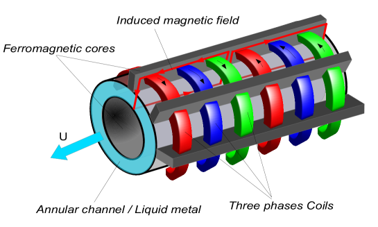
Figure 1: Schematic view of a typical linnear induction annular electromagnetic pump.

A schematic view of a typical electromagnetic pump is shown in Fig.1. In general, the liquid metal flows along an annular channel, between two concentric cylinders. A ferromagnetic core is placed on the inner side of the channel, in order to reinforce the radial component of the magnetic field created by a three-phase system of electrical currents imposed on the outer side of the channel.

In our numerical simulations, we consider the flow of an electrically conducting fluid between two concentric cylinders. $r_{i}$ is the radius of the inner cylinder, $r_{o}=r_{i}/\beta$ is the radius of the outer cylinder, and $H$ is the length of the annular channel between the cylinders. In all the simulations reported here, periodic boundary conditions are used in the axial direction.

The governing equations are the magnetohydrodynamic (MHD) equations, i.e. the Navier-Stokes equation coupled to the induction equation :

$$\rho\frac{\partial\boldsymbol{u}}{\partial t}+\rho\left(\boldsymbol{u}\cdot\boldsymbol{\nabla}\right)\boldsymbol{u}=-\boldsymbol{\nabla}P+\rho\nu\boldsymbol{\nabla}^{2}\boldsymbol{u}+\boldsymbol{j}\boldsymbol{\times}\boldsymbol{B},$$ (1)

$$\frac{\partial\boldsymbol{B}}{\partial t}=\boldsymbol{\nabla}\boldsymbol{\times}\left(\boldsymbol{u}\boldsymbol{\times}\boldsymbol{B}\right)+\frac{1}{\mu_{0}\sigma}\boldsymbol{\nabla}^{2}\boldsymbol{B},$$ (2)

where $\rho$ is the density, $\nu$ is the kinematic viscosity, $\sigma$ is the electrical conductivity, $\mu_{0}$ is the magnetic permeability, $\boldsymbol{u}$ is the fluid velocity, $\boldsymbol{B}$ is the magnetic field, and $\boldsymbol{j}=\mu_{0}^{-1}\boldsymbol{\nabla}\boldsymbol{\times}\boldsymbol{B}$ is the electrical current density.

On the cylinders, we consider infinite magnetic permeability boundary conditions, for which the magnetic field is forced to be normal to each boundary. In addition, an azimuthal electrical current $J_{\theta}$ is imposed on the outer cylinder (see part1 for more details). This external electrical current $J$ is imposed as:

$$J=J_{0}\sin\left(kz-\omega t\right)$$ (3)

where $J_{0}$ is the amplitude of the applied surface current, $\omega$ and $k=2\pi/\lambda$ are respectively the pulsation and the wavenumber of the magnetic field.

Our equations are made dimensionless by a length scale $l_{0}=\sqrt{r_{i}(r_{o}-r_{i})}$ and a velocity scale $u_{0}=c$, where $c=\omega/k$ is the speed of the TMF. The pressure scale is $p_{0}=\rho c^{2}$ and the scale of the magnetic field is $B_{0}=\sqrt{\mu\rho}c$.

The problem is then governed by the geometrical parameters $\Gamma=H/(r_{o}-r_{i})$ and $\beta=r_{i}/r_{o}$, and the following dimensionless numbers: the magnetic Reynolds number $Rm=\mu\sigma cl_{0}$, the magnetic Prandtl number $Pm=\nu/\eta$, and the Hartmann number, which controls the magnitude of the applied current, defined as $Ha=\mu_{0}J_{0}l_{0}/\sqrt{\mu_{0}\rho\nu\eta}$. Alternatively, one may define a kinetic Reynolds number $Re=Rm/Pm$ instead of $Pm$.

These equations are integrated with the HERACLES code Gonzales06 , described in the first part of this article. Typical resolutions used in the simulations reported in this article are $(N_{r},N_{Z})=[256,1024]$. For the velocity field, no-slip conditions are used at the radial boundaries. Depending on the simulations, we can either impose an inlet velocity $U_{in}$ at $z=0$, or an applied pressure gradient $P_{in}$ over the whole pump.

In our previous article, we studied a strongly idealized configuration with small Reynolds numbers ($Re=100$) and axially infinite channels. In the simulations reported in the present paper, we explore a much more turbulent configuration, with Reynolds numbers ranging from $Re=3000$ to $Re=10000$. In addition, we take into account the so-called pump inlet/outlet conditions. This means that the boundary electrical currents are applied only on one half of the computational domain (from $z=H/4$ to $z=3H/4$), so the pump has a finite size and discharges into a non-magnetized channel.

III Counter-flow instability

Figure 2 shows a typical numerical simulation obtained for $Re=5000$, $Rm=30$ and $Ha=1200$. Figure 2(a) shows an instantaneous snapshot of the structure of the axial velocity field, whereas Fig. 2(b) shows the instantaneous Laplace force. For these values of the parameters, the normalized flow rate is close to unity in most of the domain, and the bulk of the fluid is nearly pumped in synchronism with the magnetic field. Contrary to the axially infinite laminar pump studied in part1 , the velocity profile (even time-averaged) is not independent of $z$. Since the magnetic field is applied on the outer cylinder only between $z=H/4$ and $z=3H/4$, the inlet/outlet conditions lead to strong flow perturbations, with a stronger effect at the inlet boundary, as shown in Fig. 2.

In this region, the radial magnetic field is also more complex and tends to decay with the distance from the external cylinder. Another strong difference with simulations performed at smaller $Re$ is the behavior of the boundary layers. When the flow enters the active region, there is a widening of the magnetic boundary layer close to the inner cylinder, whereas a narrowing is observed close to the external boundary.

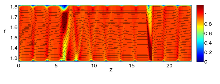
(a)

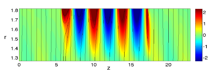
(b)

Figure 2: (a) Colorplot of the velocity field and (b) of the magnetic field for $Rm=30$, $Ha=1200$ and $Re=5000$. Streamlines and magnetic field lines are shown in black. Figure has been enlarged in the radial direction.

Fig. 3 shows the time-averaged velocity field for a larger magnetic Reynolds number ($Rm=60$) and illustrates the spatial organization of the flow. Before entering the active region ($z<H/4$), the flow exhibits a laminar structure relatively symmetrical and identical to the solutions obtained at smaller $Re$ and reported in the first part of the paper. Despite the absence of applied magnetic field in this region, note that the velocity profile is different from a classical annular Poiseuille flow. The presence of a relatively flat profile in the bulk flow and a stronger shear near boundaries is more typical of magnetized regimes.

As the velocity field is probed at larger $z$, inside the active region ($z=9$ and $z=15$), the maximum value of $U_{z}$ shifts towards the outer cylinder, leading to stronger velocity gradient close to this boundary. On the contrary, the inner boundary layer widens. This effect is not observed at smaller $Rm$, where the velocity (except in the boundary layers) is strongly homogeneous in the radial direction. Finally, outside the active region, the system comes back very rapidly to the symmetrical profile with magnetic boundary layers on each sides of the annular gap.

In addition, there is a strong perturbation as the fluid enters or leaves the active region of the electromagnetic pump. These perturbations at the inlet/outlet boundaries induce a large adverse pressure gradient inside the channel and can yield local velocities stronger than the wave speed.

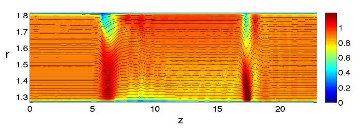
(a)

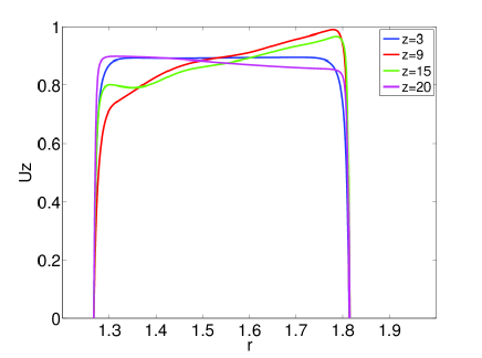
(b)

Figure 3: (a) Colorplot of the time averaged axial velocity field for run with $Rm=60$, $Ha=1200$ and $Re=5000$. (b) Corresponding profiles in the radial direction for different values of $z$.

It is important to note that despite strong fluctuations, the flow for $Rm=30$ and $Rm=60$ stays relatively homogeneous in most of the computational domain, and the total flow rate developed by the channel is very close to its maximum value.

According to the solid body model for induction pumps Galaitis76 , an instability of the flow similar to the stalling of an asynchronous motor should appear at sufficiently large $Rm$. Our numerical simulations at low $Re$ exhibit a behavior very close to the predictions. The magnetic Reynolds number is therefore further increased, from $Rm=60$ to $Rm=120$, keeping fixed $Ha=1200$ and $Re=5000$. The turbulent flow studied here develops a behavior drastically different from the stalled regime observed in the laminar case. Fig. 4(a) shows a colorplot of the averaged velocity field in such regime. Compared to the regime obtained at lower $Rm$, the flow rate developed by the channel has been strongly reduced with a total normalized flow rate around $Q\sim 0.5$. This decrease in the efficiency of the pump takes the form of a strong inhomogeneous flow in both radial and axial direction. Indeed, one can see that the fluid located close to the outer cylinder, where the surface current is applied, moves nearly in synchronism with the wave, similarly to the regime obtained at lower $Rm$. On the contrary, the inner region exhibits a strongly fluctuating negative velocity, flowing against the TMF. These negative velocities can be observed in the time averaged velocity profiles shown in Fig. 4(b). Whereas the profiles outside the pump remain Hartmann-like, inside the pump the profiles drastically change its shape, achieving negative velocities of the same order than the positive ones, for $r<1.5$. For some values of $r$, it is possible to observe positive velocities larger than the driving wave speed.

Fig. 4(c) shows the time averaged axial velocity profiles in the center of the $z$ domain for runs at different Reynolds numbers, from $Re=100$ up to $Re=10000$, at fixed $Ha=1000$. For these parameters, the inhomogeneous regime shown in Fig. 4(a) appears for the three high $Re$ number simulations as well, giving similar profiles than for $Re=5000$, although very different from the laminar case ($Re=100$).

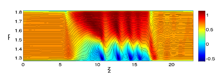
(a)

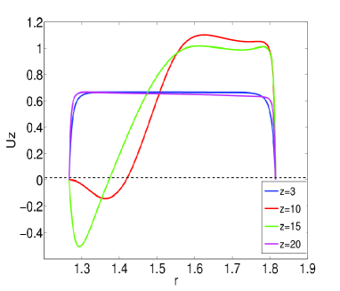
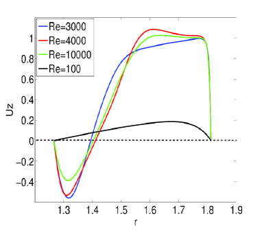
(b)

Figure 4: (a) Colorplot of the time averaged velocity field for run with $Rm=120$, $Ha=1200$ and $Re=5000$. (b) Corresponding profiles in the radial direction for different values of $z$. (c) Velocity profiles in the radial direction for runs with $Re=3000,4000$ and $10000$, for fixed $Rm=120$, $Ha=1000$. Note the difference with $Re=100$ (obtained for $Rm=120$, $Ha=100$).

A careful study of each simulation computed for different $Ha$ and $Rm$ numbers, at a fixed value of the fluid Reynolds number $Re=5000$ gives the $Ha-Rm$ parameter space shown in Fig. 5. Black circles indicate simulations similar to the one described in Fig. 2 and Fig. 3: in most of the domain, the fluid is relatively homogeneous, independent of $r$ (except close to the boundaries) and in synchronism with the wave.

Blue squares represent simulations where a very small flowrate is observed. In these runs, the flow is still homogeneous in $r$, but the velocities remain very small in comparison with the speed of the wave. This situation is reminiscent to the one observed in the first part of the article, associated with a global stalling of the pump.

Red squares correspond to the new state described in fig. 4 in which the flow becomes unstable and inhomogeneous in $r$.

This parameter space clearly differs from the one obtained in the case of laminar simulations seen in part 1, for which only one transition is observed, from homogeneous synchronism with the wave (black circles) to homogeneous stalled flow (blue squares). The difference therefore lies in the presence of inhomogeneous flows, characterized by the presence of both synchronous and stalled flows, in different parts of the channel.

It also should be noted that the parameter space does not seem to show a strong dependence on the Reynolds number, at least for $Re$ comprised between $3000$ and $10000$, as can be observed from comparison between Figs.  4(b) and (c). Nonetheless, our simulations indicate that the upper boundary of the instability pocket decreases as we decrease $Re$ (from $Ha\sim 1000$ to $Ha\sim 800$, when going from $Re=5000$ to $Re=3000$), whereas the lower boundary remains among the same values of $(Ha-Rm)$. This narrowing of the instability pocket as we decrease $Re$ is consistent with the theoretical predictions of the solid body model presented in the first part of the paper. At small values of $Re$, the parameter space of the laminar problem is divided by a single marginal stability line following $M_{b}^{c}\propto\sqrt{Re_{s}}$, where $Re_{s}=(c-u)l_{0}/\nu$ is the kinetic Reynolds number based on the slip. Here, $M_{b}^{c}=(c-u)\sqrt{\rho\mu_{0}}/B_{0}$ is the critical Alfvenic Mach number comparing the velocity of the fluid to the Alfven wave celerity at onset. It measure the ability of the fluid to expel magnetic flux from the bulk. The simulations reported in this second paper show that as $Re$ is increased, a new regime appears, opening the marginal instability line into a pocket for which both synchronous and stalled flows coexists in the bulk flow. In most of the parameter space, both boundaries of this pocket present a strong hysteresis. In our simulations, the limit between the three regimes shown in Fig. 5 was always obtained entering the instability pocket from the homogeneous solution (from black or blue points towards red points). In this fashion, the upper limit of the pocket is expected to follow the turbulent scaling $M_{b}^{c}\propto 1$ (see part I) if flux expulsion is still the mechanism involved in the generation of this new instability.

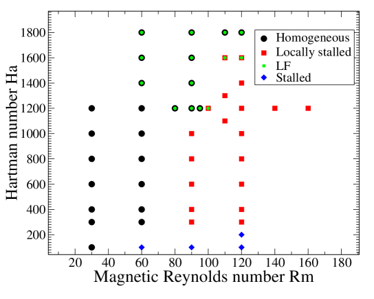
Figure 5: Parameter space $(Ha,Rm)$ explored at a given Reynolds number $Re=5000$. Black circles correspond to the stable solution depicted in Fig. 2, where the flows are homogeneous in $r$. Blue points also correspond to flows homogeneous in $r$, but associated to very small flowrates (classical stalling instability). Red squares correspond to simulations with inhomogeneous flows as the ones shown in Fig. 4. Low frequency pulsation (see text), when present, is indicated by green circles.

IV Composite model

At this point, it is interesting to compare the present high Reynolds number results with theoretical predictions and laminar simulations discussed in the first part of this article. First, the structure of the parameter space shown in Fig. 5 is very different, with the presence of two boundaries for the generation of the instability associated to an inhomogeneous flow (and the related decreased flow rate). In addition, the presence of a negative flow rate, with fluid moving backward with respect to the driving magnetic field, seems in strong contradiction with the simple usual description of MHD induction machines.

In fact, this large scale destabilization of the flow can be regarded as an effect of a local stalling of the flow, in which different regions of fluid (for different values of $r$) can be considered as several elementary electromagnetic pumps. Since the total flow rate must be equal to the sum of the flow rate in each elementary region, and if we suppose that the applied magnetic field is almost independent of $r$, the individual pumps are connected in parallel hydraulically and in series electrically. In this case, each different region is associated to identical control parameters $Rm$ and $Ha$.

The colorplot shown in Fig. 4 suggests that only the region close to the inner cylinder stalls, whereas the fluid located near the outer cylinder stays in synchronism. We therefore consider the simplest composite model containing two hydraulically parallel and electrically independent sub-channels. Suppose that channel $1$ corresponds to the quarter of the domain close to the coils (say pump $1$), while channel $2$ corresponds to the last quarter close to the inner cylinder (pump $2$). Since it corresponds to a transition zone, the central part of the fluid is not described here.

Figs. 6(a) and (b) show the evolution of the normalized flow rate $Q_{i}=\frac{1}{S_{i}}\int_{S_{i}}\frac{U_{z}}{c}dS$ of the two elementary pumps of section $S_{i}$ as a function of $Rm$ and as a function of $Ha$, respectively, as the system enters the instability region.

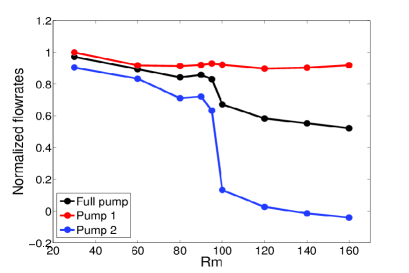
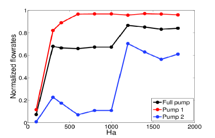
(a)                                                          (b)

Figure 6: (a) Flowrate as a function of the magnetic Reynolds number for $Ha=1200$. (b) Flowrate as a function of the Hartmann number for $Rm=90$. In both cases, the black points represent the values considering the full channel, while the red and blue lines stand for pump $1$ and pump $2$ respectively.

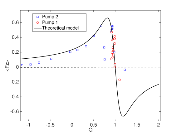
Figure 7: PQ curve for $Rm=60$, $Ha=1000$. The black line represents the theoretical model considering the flowrates obtained for the full channel, while the red and blue points stand for pump one and pump two respectively.

At small $Rm$ and relatively large $Ha$, the total flow rate (black curve) is nearly independent of $r$, yielding identical $Q_{i}$ in both sub-channels. The total flow rate then abruptly decreases for $Rm>Rm_{c}$, with $Rm_{c}\sim 90$ (see Fig. 6(a)). The evolution of the two elementary channels shows clearly that this decrease is essentially due to a stalling of the pump $2$ with a flow rate dropping to $Q_{2}\sim 0.1$, whereas the flow rate of the fluid close to the coils keeps values surprisingly close to synchronism ($Q_{1}>0.8$). The evolution of $Q_{2}$ alone is very similar to the results obtained in low-$Re$ simulations for the whole channel. In particular, the local values of the magnetic Mach number $M_{b}$ in channel $1$ are all much smaller than one, while inhomogeneous flow are generated when local $M_{b}$ in channel $2$ reaches a critical value $M_{b}^{c}\sim 0.1$. This last point highlights the fact that flux expulsion is still the physical mechanism generating the inhomogeneous flow observed here, except that it only occurs locally.

If $Ha$ is decreased at fixed $Rm$ (Fig. 6(b)), two transitions are observed. For $Ha<1200$ a first bifurcation occurs, corresponding to the one described above, i.e. the stalling of the inner region of the channel only. As $Ha$ is decreased further, a secondary bifurcation is observed, in which the flow rate in the outer region, close to the coils, also drops to zero. This second transition is closer to the behavior observed for asynchronous motors, and corresponds to a global stalling of the flow.

It is instructive to compute the typical Pressure-Flow rate characteristic curve of the system. To do this, a set of simulations for parameters outside the instability pocket ($Ha=1000$, $Rm=60$) was performed, imposing an increasing flowrate to the whole system, from $Q=-1.5$ to $Q=1.5$. For each run, time and space averaged velocity, pressure drop and Laplace force were measured inside the whole channel, but also in each region corresponding to the two individual pumps.

Fig. 7 shows the Laplace force as a function of the flowrate in each sub-channel, computed only for $7<z<15$, in order to exclude the fluctuations occurring at the inlet/outlet boundaries. The most striking result is the fact that although the $PQ$ curve for the total channel in this turbulent regime is more complex than the theoretical one, each elementary channel seems to lie on a single common curve. Once again, it must be kept in mind that there is a variation of the Laplace force with $r$ as we move along the sub-channels, so the pumps are not fully in series electrically. As a consequence, it appears from Fig. 7 that the fluid in region $1$(near the coils) always moves in synchronism, while pump $2$ can either be in synchronism (upper stable region of the parameter space) or exhibit smaller velocity.

This reinforces the interpretation of two hydraulically parallel pumps, with similar control parameters $Rm$ and $Ha$ but lying on different regions of their characteristic. More exactly, for a given imposed total flow rate $Q$, there is always one solution corresponding to both sub-channels delivering identical discharge. When $Q$ is large enough, this solution is the only one and both sub-channels flow in synchronism with the wave (on the descending branch of the $PQ$-curve). As the total flow rate decreases, both elementary pumps move along their characteristic until the maximum of the curve is reached. Below this critical value of $Q$, a second solution corresponding to different elementary discharges is possible, the total flow rate being the sum of the two elementary ones. In this regime, Fig. 7 shows that the functioning point of channel $1$ (red dots) is always located on the descending branch of the PQ curve, close to synchronism, whereas only the internal part of the fluid (’pump $2$’) moves on the ascending branch. For instance, when the imposed flow rate is $Q=0.2$, the fluid located in the inner region exhibits a strongly negative flow rate ($Q_{2}=-0.6$) in order to compensate the large positive flow rate $Q_{1}=0.9$ close to the coils and satisfy incompressibility. In order to highlight this interpretation, we added to Fig. 7 the solution expected in the framework of simple solid-body theory (eq. $2.17$ in part1 , with $H=2.7$ and $R=5.6$).

However, there are also important differences between this simple composite model and our numerical simulations. First, the assumption of only two pumps in parallel is very restrictive. For instance, this description ignore the central part of the annulus, or the boundary layers in which the velocity vanishes. In addition, the magnetic field being imposed only at the boundaries, the simulations involve a local Hartmann number which depends on the radial direction, in contradiction with the assumption of pumps connected in series electrically. Finally, some of the numerical points in Fig. 7 significantly differ from the theoretical curve (in particular the presence of two maxima for the Lorentz force in channel $2$, at $Q_{2}\sim 0.7$ and $Q_{2}\sim 0.9$). This departure finds its origin in the fact that very close to synchronism, flux expulsion vanishes and electrical currents generated at the outer cylinder can propagate easier through the radial gap, thus leading to an amplification of the induced field close to the inner cylinder. This behavior is reminiscent of the localized nature of the forcing, which is not described by the classical solid body theory.

The above description is almost equivalent to the composite model discussed in Galaitis76 . In this article, Gailitis and Lielausis proposed that an electromagnetic pump can be modeled, in the limit of small gap, as a combination of many elementary pumps connected in $\phi$, therefore predicting a loss of homogeneity of the velocity distribution along the azimuthal direction above some critical value of the magnetic Reynolds number. In its simplest form, this model involves two elementary pumps, similarly to the results reported here. Even in axisymmetric configurations such as the simulations reported here, a similar mechanism occurs, except that the loss of homogeneity is achieved in the radial direction instead. This inhomogeneous structure, associated to a strong radial shear, is likely to produce destabilization of the flow in the azimuthal direction. Although additional 3D runs will be necessary to conclude, this destabilization would provide a new scenario, different from the mechanism proposed in Galaitis76 , for the occurence of non-axisymmetric states in such annular induction pumps.

V Low Frequency pulsation

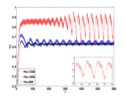
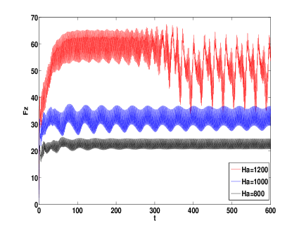
(a)                                                          (b)

Figure 8: (a) Time series of the normalized axial velocity $V_{z}$ in the central part of the pump, averaged in $r$, for $Rm=90$ and various values of $Ha$. The inset shows an enlarged view of the pulsation for $Ha=1200$. (b) The same for the Lorentz force. As $Ha$ is increased, a low frequency pulsation develops in both fields.

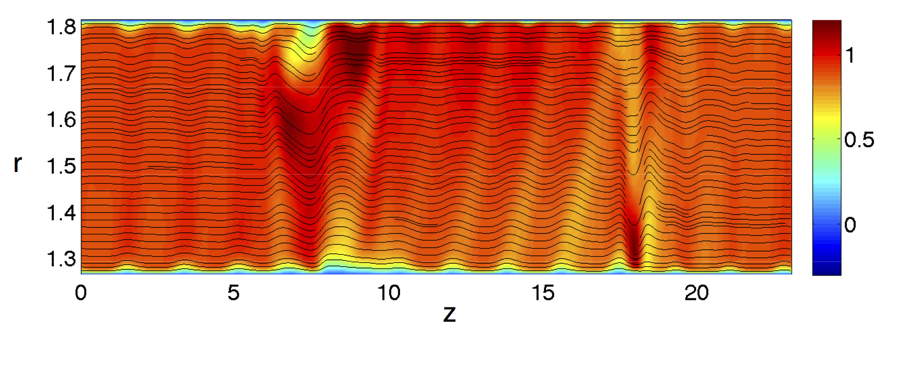
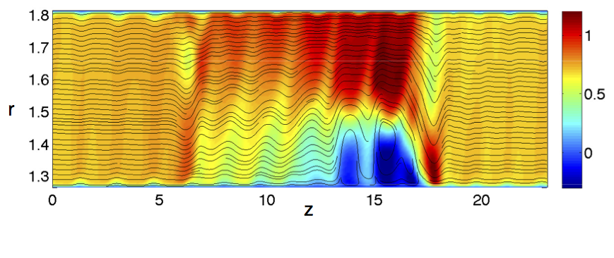
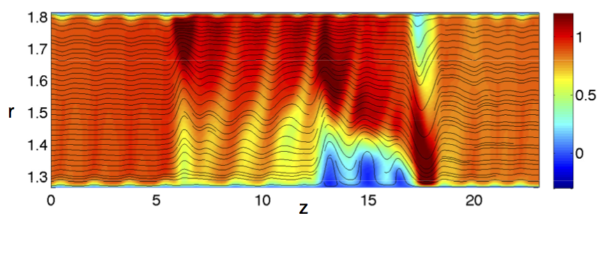
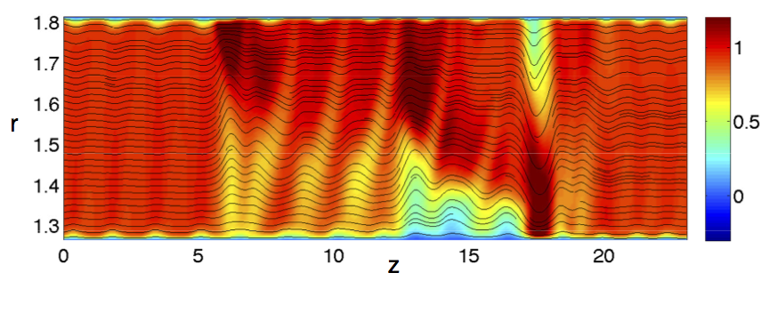
Figure 9: Colorplot of four different snapshots of the axial velocity for run with $Rm=90$, $Ha=1200$. A vortex near the upper boundary appears and disappears (from top to bottom) following a cycle with $\tau\sim 30$.

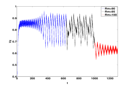
Figure 10: Time series of the axial velocity $V_{z}$ in the central part of the pump, averaged in $r$, for fixed different values of Rm.

Despite strong turbulent fluctuations, the large scale vortex flow observed in Fig. 4 is statistically stationary when the system is located deep inside the instability pocket (represented by red dots in Fig. 5). However, a more complex time behavior is systematically observed close to the marginal stability line. Green symbols in Fig. 5 indicate solutions in which a periodic modulation of the flow rate is obtained. Figs. 8(a) and (b) show the time series for the $z$ component of velocity field and Lorentz force for runs performed at $Rm=90$ and different values of $Ha$. The pulsation due to the forcing, at twice the wave frequency, is clearly visible on both fields for all the values. As $H$ is increased above $H=800$, a slower modulation, associated to a typical frequency one order of magnitude larger than the driving frequency, develops. As the applied field is increased, the oscillation becomes strongly non-linear, as this dynamics exhibits slowing down close to synchronism, as indicated in the inset of Fig. 8(a).

As shown in Fig. 5, this Low Frequency (LF) pulsation occurs both inside and outside the instability pocket (for instance, at $Rm=60$, $Ha=1400$, or at $Rm=120$, $Ha=1600$, as indicated by green points in Fig.5), but always close to the marginal stability line. Fig. 9 shows snapshots of the flow at four different times during the oscillation shown in the inset of Fig. 8(a). It can be seen that this regime corresponds to localized vortices, which periodically appear near the pump outlet with decreasing amplitude until they disappear.

The appearance of this regime displays a strong hysteresis, and can exhibit more complex dynamics. Fig. 10(a) shows the time evolution of the axial velocity $V_{z}$ as $Rm$ is increased (starting each simulation using as initial condition the output from the previous one) at a fixed Hartmann number $Ha=1200$. At $Rm=90$, the pulsation appears with a single frequency roughly ten times the frequency driving. As $Rm$ is increased beyond $Rm=95$, a second frequency appears in the spectrum, whereas for $Rm=100$, the LF pulsation goes back to a single frequency. For this value of $Rm$, the system is inside the instability pocket, where the vortices are statistically stationary (red points in Fig.5).

Such a Low Frequency pulsation has been reported both in experiments and simulations with comparable values Araseki04 . In this last reference however, the pulsation was associated with a loss of homogeneity of the fluid in the azimuthal direction when the forcing was non-axisymetric. The above results show that such a behavior may be generated even in axisymetric configuration.

VI Discussion and conclusion

In this article, we have extended the numerical study presented in the first part, describing an MHD flow driven by a travelling magnetic field in an annular channel, and aiming to describe linear annular induction electromagnetic pumps. Here, we report results using larger values of the flow Reynolds numbers, and also introducing the presence of inlet/outlet boundary conditions in the axial direction, giving a better description of experimental configurations.

For the turbulent case studied here, we have shown that the stalling instability previously described for laminar flows takes the form of a loss of homogeneity in the flow, for which a strongly negative velocity appears in a given region of the channel. We have identified this behavior as a local stalling of the flow, characterized by the coexistence of two regions of fluids with very different velocity and induced magnetic field.

This is consistent with a simple model of several pumps operating in parallel hydraulically, although not electrically in series. This arises from the fact that, since the magnetic field is imposed only at the boundaries, the simulations involve a local Hartmann number which depends on the radial direction. As a consequence, the inner part of the fluid always becomes unstable before the region of fluid close to the outer cylinder, where the electrical currents are imposed. In this case, the flow exhibits a Poiseuille-like profile close to the inner cylinder, and an Hartmann-like profile close to the outer cylinder.

The use of 2D simulations allowed us to explore a large region of the parameter space $(Ha,Rm,Re)$. At large $Re$, the single marginal stability curve observed for laminar flows is replaced by a pocket of instability involving inhomogeneous velocity profiles. Although more simulations are necessary to give a definitive conclusion, our results suggest that the upper boundary of the instability pocket is consistent with the scaling involving the Alfvenic Mach number $M_{b}>$constant . As explained in the first part of our article, this scaling law indicates that magnetic flux expulsion is responsible for the loss of synchronism close to the inner side of the pump, where the magnetic field, and therefore the force, are weaker. It is important to note that an adverse pressure gradient is necessary for a pump to lie on the negative part of its characteristic curve. In our turbulent simulations, such a load is created by the inlet/outlet conditions at the ends of the pump.

Finally, consistently with previous experimental and numerical results on annular linear induction EMPs, we have also observed the appearance of a periodic modulation of the fields with a typical frequency approximately $30$ times smaller than the applied external frequency. This modulation takes here the form of axisymmetric pulsating vortices which systematically occur close to the upper marginal stability line of the reversed flow instability.

It is now interesting to compare these numerical results to existing experimental configurations. Medium size EMPs can reach magnetic Reynolds numbers higher than $10$ and Hartmann numbers larger than $800$ (with our definition of $Rm$ and $Ha$), while the largest EMPs reported in the literature correspond to $Rm>50$ and $Ha>10^{5}$ Ota04 ; Araseki04 . This suggests that the axisymmetric loss of homogeneity reported here may be relevant to experimental configurations using similar types of forcing, in which the electrical currents are applied only on one side of the pump. In this perspective, it would be interesting to understand how this intrinsically axisymmetric instability is modified by the presence of electrical currents on both sides of the annular channel. Similarly, secondary bifurcations towards non-axisymmetric states should be expected in both single-sided or double-sided configurations, and the study of this fully 3d states will be reported in a future work.

- (1)
- (2) Gailitis A. and O. Lielausis, Instability of homogeneous velocity distribution in an induction-type mhd machine, Magnetohydrodynamics, 1, 69-79 (1976). Translation from Magnitnaya Gidrodinamika 1, 87-101 (1975).
- (3) Kirillov, I.R., Ogorodnikov, A.P., Ostapenko, V.P. ,Local characteristics of a cylindrical induction pump for Rms larger than 1 , English translation from Magnitnaya Gidrodinamika 2, 107- 113 (1980)
- (4) Karasev, B. G., Kirillov, I. R., Ogorodnikov, A. P., 3500 m3/h MHD pump for fast breeder reactor , Liquid Metal Magnetohydrodynamics. Kluwer, Dordrecht, pp. 333-338 (1989).
- (5) Araseki, H., Kirillov, I., Preslitsky, G., Ogorodnikov, A. P., Double-supply-frequency pressure pulsation in annular linear induction pump. Part I. Measurement and numerical analysis. , Nucl. Engin. and Design, 195, 85-100 (2000)
- (6) Araseki, H., Kirillov, I., Preslitsky, G. V., Ogorodnikov, A. P., Magnetohydrodynamic instability in annular linear induction pump:: Part I. Experiment and numerical analysis , Nucl. Engin. and Design, 227, 29-50 (2004)
- (7) Gonzales, M., Audit, E., Huynh, P., HERACLES: a three-dimensional radiation hydrodynamics code , Astronomy and Astrophysics, 464, 429-435 (2006).
- (8) Gissinger, C., Rodriguez Imazio, P., Fauve, S., Instability of electromagnetically driven flows, part I Phys. Fluids (2015)
- (9) Ota, H., Development of 160 m3/min large capacity sodium-immersed self-cooled electromagnetic pump , J. Nucl. Sci. Tech., 41, 511-523 (2004)
- (10) Andreev, A. M. et al, Results of an experimental investigation of electromagnetic pumps for the BOR-60 facility , Magnitnaya Gidrodinamika, 1, 617 (English translation) (1988)
- (11) Liu, W., Goodman, J., Ji, H., Simulations of magnetorotational instability in a magnetized Couette flow , Astrophys. J., 643, 306 (2006).
- (12) W. Liu, Numerical study of the magnetorotational instability in Princeton MRI experiment, Astrophys. J., 684, 515 (2008).
- (13) Gissinger, C., Ji, H., Goodman, J. , The role of boundaries in the Magnetorotational instability , Phys. Fluids., 24, 074109 (2012).
- (14) Kamkar, H. & Moffatt, H. K., A dynamic runaway effect associated with flux expulsion in magnetohydrodynamic channel flow , J. Fluid Mech., 121,107-122 (1982)