Time resolution of the plastic scintillator strips with matrix photomultiplier readout for J-PET tomograph

Abstract

Recent tests of a single module of the Jagiellonian Positron Emission Tomography system (J-PET) consisting of 30 cm long plastic scintillator strips have proven its applicability for the detection of annihilation quanta (0.511 MeV) with a coincidence resolving time (CRT) of 0.266 ns. The achieved resolution is almost by a factor of two better with respect to the current TOF-PET detectors and it can still be improved since, as it is shown in this article, the intrinsic limit of time resolution for the determination of time of the interaction of 0.511 MeV gamma quanta in plastic scintillators is much lower. As the major point of the article, a method allowing to record timestamps of several photons, at two ends of the scintillator strip, by means of matrix of silicon photomultipliers (SiPM) is introduced. As a result of simulations, conducted with the number of SiPM varying from 4 to 42, it is shown that the improvement of timing resolution saturates with the growing number of photomultipliers, and that the 2 x 5 configuration at two ends allowing to read twenty timestamps, constitutes an optimal solution. The conducted simulations accounted for the emission time distribution, photon transport and absorption inside the scintillator, as well as quantum efficiency and transit time spread of photosensors, and were checked based on the experimental results. Application of the 2 x 5 matrix of SiPM allows for achieving the coincidence resolving time in positron emission tomography of $\approx$ 0.170 ns for 15 cm axial field-of-view (AFOV) and $\approx$ 0.365 ns for 100 cm AFOV. The results open perspectives for construction of a cost-effective TOF-PET scanner with significantly better TOF resolution and larger AFOV with respect to the current TOF-PET modalities.

Keywords: scintillator detectors, J-PET, positron emission tomography, timing resolution

1 Introduction

There is a continued interest in improving time resolution of scintillator detectors. Such improvements are especially challenging in case of the registration of low energy gamma quanta where the time resolution is limited by the low statistics of scintillation photons.

Superior time resolution for registration of low energy gamma quanta is of crucial importance in the nuclear medicine applications as e.g. in positron emission tomography (PET), where the new generation of PET scanners utilizes for the image reconstruction differences between time of flight (TOF) of annihilation quanta from the annihilation vertex to the detectors ( Conti 2009, Humm et al 2003, Karp et al 2008, Townsend 2004, Moses Derenzo 1999, Moses 2003, Conti Eriksson 2009 ).

In order to improve the TOF resolution and to increase a geometrical acceptance of the PET scanners we are developing a J-PET detection system ( Moskal et al 2011 2014 2015, Raczynski et al 2014 2015 ). The system is based on long strips of plastic scintillators which are characterized by better timing properties than the inorganic scintillator crystals used in the state of the art PET scanners ( Conti 2009, Humm et al 2003, Karp et al 2008, Townsend 2004, )

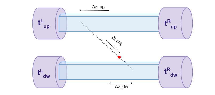
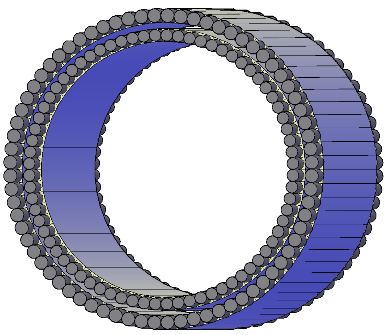
Figure 1: (Left) Schematic view of the two detection modules of the J-PET detector. A single detection module consists of a scintillator strip read out by two photomultipliers. A single event used for the image reconstruction includes information about times of light signals arrival to the left (L) and right (R) ends of the upper (up) and lower (dw) scintillators (t${}^{R}_{up}$, t${}^{L}_{up}$, t${}^{R}_{dw}$, t${}^{L}_{dw}$). A filled red dot inside the figure indicates a place of e⁺e^- annihilation. $\Delta{z}$ denotes the position of the interaction point along the scintillator, and $\Delta{LOR}$ indicates the position of annihilation along the line-of-response (LOR). More details are explained in the text. (Right) Schematic visualization of an example of two detection layers of the J-PET detector. Each scintillator strip is aligned axially and read out at two ends by photomultipliers.

Left panel of Fig. 1 shows a schematic view of two detection modules of the                                                                                          J-PET detector, where (similarly as described in the reference (Nickles et al 1978)) the time of the interaction (hit-time) of gamma quantum in the scintillator ($t_{hit}=(t^{L}+t^{R})/2$) is calculated as an arithmetic mean of times at left ($t^{L}$) and right ($t^{R}$) side of the strip. The position of interaction along the strip (axial hit position) may be in the first approximation calculated as $\Delta z$ = ($t^{L}-t^{R}$) $v$ / 2, where $v$ denotes the speed of light signals in the scintillator strip. For example for plastic strips with cross section of 0.5 cm x 1.9 cm the effective light signal velocity is equal to $v$ = 12.2 cm/ns (Moskal et al 2014). Thus, in the case of strips with the length of 30 cm characterized with the hit-time resolution of 0.188 ns (FWHM) the axial position resolution amounts to about 2.3 cm (FWHM) (Moskal et al 2014). The position along the line-of-response ($\Delta LOR$) between two strips (e.g. up and down shown in the left panel of Fig. 1) is calculated as ($\Delta LOR=(t_{hit}^{up}-t_{hit}^{dw})c/2$, where $c$ denotes the speed of light. The hit-time and hence also axial position resolution may still be improved e.g. by probing photomuliplier pulses in the voltage domain by a newly developed electronics (Palka et al 2014), and by applying in the reconstruction the compressing sensing theory (Raczynski et al 2014,2015) and the library of synchronized model signals (Moskal et al 2015). The timing resolution, as it is introduced hereafter in this article, can be also improved by making a readout allowing to record time-stamps from larger number of photons compared to the case of the vacuum tube photomultipliers.

Due to the relatively low costs of plastic scintillators and their large light attenuation length (in the order of 100 cm) it is possible to construct a detector with a long axial field-of-view in a cost effective way. This feature makes the J-PET detector competitive to the present solutions as regards the whole-body imaging. One of the possible arrangements of the scintillator strips in the J-PET scanner is visualized in the right panel of Fig. 1. Such alignment permits to use more than one detection layer thus increasing the efficiency of gamma quanta registration.

Plastic scintillators were not used so for as possible detectors for PET imaging due to the negligible probability of the photoelectric effect and lower detection probability with respect to the inorganic crystals. With the plastic scintillators the detection of 0.511 MeV gamma quanta is based in practice only on the Compton scattering. In Fig. 2 we show a distribution of Compton scattered electron energy for (i) the energy of gamma quanta reaching the detector without scattering in the patient’s body, (ii) after the scattering through an angle of 30 degrees and (iii) after scattering through an angle of 60 degrees. The presented distributions show that in order to limit registration of gamma quanta scattered in the patient to the range from 0 to about 60 degrees (as it was applied earlier e.g. in some LSO or BGO based tomographs (Humm et al 2003)), one has to use an energy threshold of about 0.2 MeV (Moskal et al 2012). The scatter fraction can be further reduced at the expense of the sensitivity, yet it should be noted that its suppression to the level achievable in the newest LSO based scanners with the energy window of 0.440-0.625 MeV (Surti et al 2007) is questionable. However, for the quantitative statement, more detailed investigations are needed.

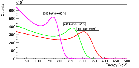
Figure 2: Energy distribution of electrons scattered via the Compton process by gamma quanta with energies shown in the plot. The shown spectra include energy deposition resolution determined for the 30 cm long strips of the J-PET detector which is equal to $\sigma(E)/E=0.044/\sqrt{E(MeV)}$ (Moskal et al 2014).

Application of 0.2 MeV threshold suppresses also to the negligible level signals due to the secondary Compton scattering in the detector material (Kowalski et al 2015). So far we have obtained 0.188 ns ($FWHM$) of hit-time resolution for the registration of 0.511 MeV annihilation quanta by means of 30 cm long strips of plastic scintillators read out at both ends by vacuum tube photomultipliers (Moskal et al 2014). The experiment was performed using a collimated beam of annihilation quanta from the ${}^{68}Ge$ isotope placed inside a lead collimator with a 1.5 mm wide and 20 cm long slit. A dedicated mechanical system allowed us to irradiate the tested scintillator at the desired position. A coincidence registration of signals from the tested module and the reference detector on the other side of the collimator ensured selection of annihilation gamma quanta. A tested module consisted of a BC-420 plastic scintillator (Saint Gobain Crystals) with dimensions of 0.5 cm x 1.9 cm x  30 cm connected optically at the ends to the Hamamatsu photomultipliers R5230 (Hamamatsu). The experimental setup and results of the measurements are described in detail in reference (Moskal et al 2014).

In principle, information about a time of interaction of gamma quantum in the scintillator is carried by all emitted scintillation photons. However, in practice in the typical detectors, only few first registered photons, contributing to the leading edge of the electrical signal generated by the photoelectric converters, are utilized in the determination of the onset of these signals and hence in the determination of the time of the gamma quantum interaction. This is also the case for the scintillator strips in the current version of the J-PET detector (see upper part of Fig. 3), where the time of the interaction is determined as an arithmetic mean of times at which electric signals generated by photomultipliers attached to both ends cross a preset threshold voltage. Therefore, the time resolution may be improved by making a readout allowing to record timestamps from larger number of photons arriving at the scintillator edge. There are first attempts to register all timestamps using arrays of single-photon avalanche diodes (Meijlink et al 2011), but presently the registration of arrival time of all photons with a good time resolution at large areas is still rather impractical. It is, however, important to stress that the intrinsic timing resolution limit is approached already when using only about 20 timestamps from first detected photons (Seifert et al 2012).

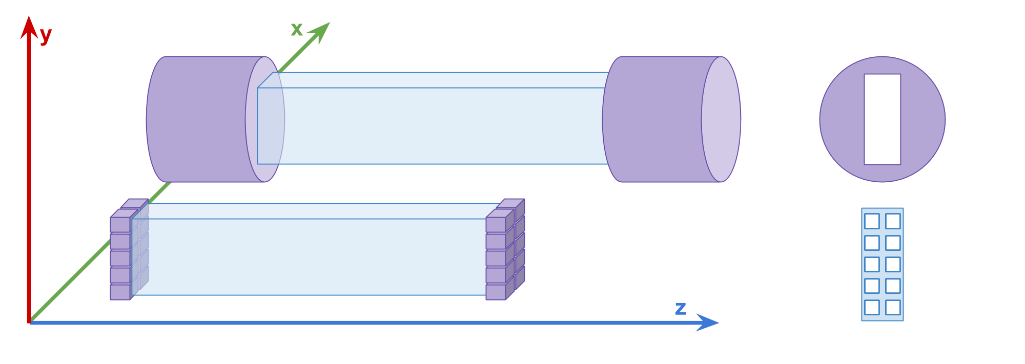
Figure 3: Upper scheme indicates a single module of the J-PET detector consisting of the scintillator strip read out on two sides by vacuum tube photomultipliers (Moskal et al 2014). Lower part of the figure indicates a scheme of an exemplary multi-SiPM readout allowing for determination of timestamps of 20 detected photons (ten on each side). Right panel of the figure shows arrangement of photomultipliers. Geometrical overlap between the scintillator and the photosensitive part of the photomultipliers is marked as white rectangles.

In this article we study the possibility of improving the time resolution for the large size detectors (few tens of centimeters) by registration of timestamps from several photons. This may be realized by preparing a readout in the form of an array with several SiPM photomultipliers as it is indicated in the lower part of Fig 3. In such a case, a set of all registered photons is divided into several subgroups and a time of the registration of the first photon in each subgroup is recorded. This allows to construct estimators of the time of gamma quantum interaction based on the number of timestamps equal to the number of SiPM photomultipliers.

In the following sections, first we estimate time resolution limits for infinitesimally small detector making an idealistic assumption that the time of arrival of each photon can be measured and used for the estimation of the time of gamma quantum interaction. We use Fisher information from all emitted photons and calculate the Cramér-Rao lower limit ( Seifert et al 2012, De Grot 1986 ) which is independent of the estimator used for the time resolution determination. Such estimations of the lower bound for the time resolution have been published recently (Seifert et al 2012) for small size crystals, taking into account the transit time spread of photomultipliers and neglecting the spread of the transit time inside scintillators. In this article we extend these investigations to the plastic scintillators strips with the length of up to 100 cm and include in the estimations the transit time spread due to the propagation of photons in scintillator strips as well as the transit time spread of photomultipliers. Further on we determine the lower bounds for the time resolution using a weighted mean of timestamps as an estimator of the time of the gamma quantum interaction. Next, we describe parameters used in the realistic simulations, including time distribution of photons emitted in ternary plastic scintillators, losses and time spread of photons due to their propagation through the scintillator, as well as quantum efficiency and transit time spread of photomultipliers. We test the simulation procedures by comparing simulated and experimental results for the BC-420 plastic scintillator read out at two ends by Hamamatsu R5320 photomultipliers. Section 7 contains description of the main idea of this article where the estimator of the time of the gamma quantum interaction is defined based on the time ordered set including timestamps from first photons registered by the matrix of SiPM converters. In this section we perform realistic simulations for the BC-420 scintillator strip and various configurations for the arrays of S12572-100P Hamamatsu silicon photomultipliers. Finally we estimate time resolution as a function of the scintillator length for the multi-SiPM readout allowing to determine timestamps of 20 photons. The results are compared to the resolutions achievable with the traditional readout with the vacuum tube photomultipliers.

The light yield of plastic scintillators amounts to about 10000 photons per 1 MeV of deposited energy. Annihilation gamma quanta (0.511 MeV) used for the positron emission tomography interact with plastic scintillators predominantly via Compton scattering (Szymanski et al 2014), and therefore may deposit maximally an energy of 0.341 MeV (2/3 of electron mass). This corresponds to the emission of about 3410 photons. On the other hand, in order to decrease the noise due to the scattering of gamma quanta inside a patient body a minimum energy deposition of about 0.2 MeV is required (Moskal et al 2012). Therefore, number of emitted photons discussed hereafter in this article includes the range from 2000 to 3410 photons.

2 Estimator of hit-time resolution (variance)

A single detection module considered in this article consists of the plastic scintillator strip connected at two ends to photomultipliers (see Fig. 3). We assume that the gamma quantum or any other particle of interest interacts in the scintillator at time $\Theta$. We consider the resolution for the reconstruction of the value of $\Theta$ based on time measurement of signals generated by photosensors attached to two scintillator ends. For practical reasons, if applicable, we use notation analogous to the one introduced in references (Seifert et al 2012).

In general, timestamps of all photons detected at the left ($t^{L}_{1},t^{L}_{2},...,t^{L}_{N_{L}}$) and at the right side ($t^{R}_{1},t^{R}_{2},...,t^{R}_{N_{R}}$) of the scintillator may be used for the estimation of the time of the interaction $\Theta$. It is advantageous to order the sets of timestamps according to ascending time such that: ($t^{L}_{(1)}\leq t^{L}_{(2)}\leq...\leq t^{L}_{(N_{L})}$) and ($t^{R}_{(1)}\leq t^{R}_{(2)}\leq...\leq t^{R}_{(N_{R})}$), where indices in brackets indicate timestamps from the ordered set. The $t_{(i)}$ element in the ordered set is referred to as i-th order statistic (Seifert et al 2012). After ordering, the timestamps on one side become correlated but the ordered set allows for the simple and intuitive estimation of time difference between the signal arrivals to the ends of the scintillator:

$$\Delta t_{(i)}=t^{L}_{(i)}-t^{R}_{(i)},$$ (1)

as well as interaction time $\Theta$ which may be estimated by:

$$\Theta_{(i)}=\frac{t^{L}_{(i)}+t^{R}_{(i)}}{2}+const_{(i)},$$ (2)

where $const_{(i)}$ is subject to calibration and for simplicity, but without loss of generality, it will be omitted in the further considerations. Distributions of ordered timestamps at one side (e.g. $t^{L}_{(i)}$ and $t^{L}_{(j)}$ for $i\neq j$) are correlated and not identical. However, distributions for the same order statistics at left and right side ($t^{L}_{(i)}$ and $t^{R}_{(i)}$) are uncorrelated since the ordering at left side was done independently of the ordering at right side. Hence, it follows that variances of $\Delta t_{(i)}$, and $\Theta_{(i)}$ may be expressed as:

$$\sigma^{2}(\Delta t_{(i)})=\sigma^{2}(t^{L}_{(i)})+\sigma^{2}(t^{R}_{(i)})-2cov(t^{L}_{(i)},t^{R}_{(i)})=\sigma^{2}(t^{L}_{(i)})+\sigma^{2}(t^{R}_{(i)}),$$ (3)

$$\sigma^{2}(\Theta_{(i)})=\frac{1}{4}\left(\sigma^{2}(t^{L}_{(i)})+\sigma^{2}(t^{R}_{(i)})+2cov(t^{L}_{(i)},t^{R}_{(i)})\right)=\frac{1}{4}\left(\sigma^{2}(t^{L}_{(i)})+\sigma^{2}(t^{R}_{(i)})\right).$$ (4)

The above equations imply that:

$$\sigma^{2}(\Delta t_{(i)})=4\sigma^{2}(\Theta_{(i)})=\sigma^{2}(t^{L}_{(i)})+\sigma^{2}(t^{R}_{(i)})$$ (5)

We have checked this supposition by numerical simulations for the probability density distributions of emission times considered in this article. Therefore, as regards the variance, it is sufficient to study properties of only one of these estimators. Moreover, in order to facilitate direct comparison with results published in the field of TOF-PET we will express resolution as FWHM of coincidence resolving time (CRT), where coincidence resolving time determined for i-th order statistic will be referred to as CRT_(i). It should be, however, noted that in general, even though $t^{L}_{(i)}$ and $t^{R}_{(i)}$ are uncorrelated, the $\Delta t_{(i)}$ and $\Theta_{(i)}$ may be correlated since cov($\Delta t_{(i)}$,$\Theta_{(i)}$) = ($\sigma^{2}(t^{L}_{(i)})$ - $\sigma^{2}(t^{R}_{(i)})$)/2 is equal to zero only if the emission point is in the center of the detector because only in this case the $t^{L}_{(i)}$ and $t^{R}_{(i)}$ are identically distributed.

In next sections we define the emission time distribution for the plastic scintillators and estimate the Cramér-Rao lower limit for the achievable time resolution. Further on we will simulate time resolution for each order statistics $\Delta t_{(i)}$ separately, and we will test the variance of the weighted mean of $\Delta t_{(i)}$ values showing that such estimator of $\Delta t$ allows to reach significantly better resolution than achievable with single order statistics.

3 Emission time distributions

In case of the ternary plastic scintillators, as e.g. BC-420 (Saint Gobain Crystals) and its equivalent EJ-230 (Eljen Technology) used in the J-PET detector, the distribution of the time of the photon emission followed by the interaction of the gamma quantum at time $\Theta$ can be well approximated by the following convolution of gaussian and exponential terms (Moszynski Bengtson 1977 1979):

$$f(t|\Theta)=K\int_{\Theta}^{t}{(e^{-\frac{t-\tau}{t_{d}}}-e^{-\frac{t-\tau}{t_{r}}})\cdot e^{-\frac{(\tau-\Theta-2.5\sigma)^{2}}{2\sigma^{2}}}d\tau},$$ (6)

where the gaussian term with the standard deviation $\sigma$ reflects the rate of energy transfer to the primary solute, whereas $t_{r}$ and $t_{d}$ denote the average time of the energy transfer to the wavelength shifter, and decay time of the final light emission, respectively (Moszynski Bengtson 1979). K stands for the normalization constant ensuring that $\int_{\Theta}^{+\infty}f(t|\Theta)dt=1$. We have set $t_{d}=1.5$ ns and treated $t_{r}$ and $\sigma$ as a phenomenological parameters and adjusted their values to: $t_{r}=0.005$ ns, $\sigma=0.2$ ns in order to describe the properties of the light pulses from the BC-420 scintillator i.e. rise time of 0.5 ns, decay time $t_{d}~{}=~{}1.5$ ns and FWHM of 1.3 ns (Saint Gobain Crystals). The resultant distribution of the emission time is indicated by the black solid line in Fig. 4. Other lines in this figure correspond to time distributions of photons in the scintillator with the cross section of 0.5 cm x 1.9 cm simulated at various distances from the interaction point. These distributions will be used in the next section for the estimation of the lower limits of the achievable time resolutions.

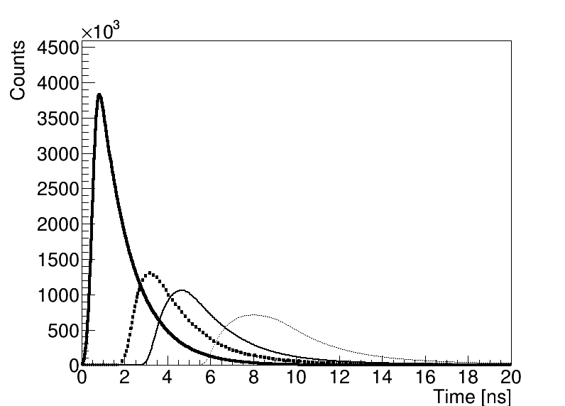
Figure 4: Thick solid line denotes the time distribution for photons simulated according to the formula 6 describing the probability density distribution for ternary plastic scintillators with parameters adjusted to the properties of BC-420 scintillator. Thick dashed line indicates distribution at 30 cm from the interaction point, thin solid at 50 cm, and thin dashed at 100 cm. These probability density distributions were simulated taking into account the time of photons propagation through a given distance along the scintillator with cross section of 0.5 cm x 1.9 cm. Simulations are described in greater details in the Appendix.

4 Cramér-Rao lower limit on the resolution of hit-time reconstruction

The time resolution achievable with the scintillator detectors is limited by the optical and electronic time spread caused by the detector components, and by the time distribution of photons contributing to the formation of electric signals. The latter depends on the number of registered photons and is referred to as the photon counting statistics (Seifert et al 2012). Limitations of the time resolution due to the photon counting statistics have been studied in detail e.g. in refs.( Seifert et al 2012,2012b), Spanoudaki Levin 2011, Fishburn et al 2010 ) and the comprehensive account on this topic may be examined e.g. in ref.(Seifert et al 2012). To large extent this research is driven by the endeavor to improve the timing properties of the PET systems ( Conti Eriksson 2009, Moszynski et al 2011, Schaart et al 2009,2010, Kuhn et al 2006, Lecoq et al 2013), and therefore so far the investigations concentrated on the small size crystal scintillators. In the recent work a detailed elaboration of the lower bound for time resolution has been published for most kinds of available crystal scintillators (Seifert et al 2012). The estimation included transit time spread of photomultipliers but the spread due to the transport of photons inside the scintillators was neglected. This was justified since only small size crystals (in the order of 1 cm or smaller) were considered. Here, inspired by the new solution for the PET system based on plastic scintillators (Moskal et al 2011,2014,2015, Raczynski et al 2014,2015), we extend the studies of Seifert and coauthors (Seifert et al 2012) from the small size crystals to the large size plastic scintillators. In this section we estimate the lower limit of the time resolution achievable with scintillator strips of up to 100 cm assuming ideal electronic systems, and further on in the following sections we describe results of realistic simulations conducted taking into account both photon transport in scintillator material and transit time spread in photomultipliers.

The variance of any unbiased estimator $\Xi$ of the hit-time $\Theta$ satisfies the Cramér-Rao inequality (De Groot 1986, Seifert et al 2012):

$$var(\Xi)\geq\frac{1}{I_{N}(\Theta)},$$ (7)

where $I_{N}(\Theta)$ denotes the Fisher information concerning $\Theta$ in the set of N randomly chosen timestamps. This very general formula enables calculation of the lower bound of the variance of unbiased estimator. In case of point estimation of a parameter it quantitatively informs about the estimation efficiency and whether there is room for improvement. Knowing the probability density distribution of the photon registration time t following the gamma quantum interaction time $\Theta$: $f(t|\Theta)$, the Fisher information in the sample of N independent timestamps reads (De Groot 1986, Seifert et al 2012):

$$I_{N}(\Theta)=N\int_{-\infty}^{+\infty}\frac{(\frac{\partial}{\partial\Theta}f(t|\Theta))^{2}}{f(t|\Theta)}dt$$ (8)

Fig. 5 shows the lower limit of the time resolution estimated as a function of the number of registered photons N based on relations 7 and 8. Thick-solid line shows results assuming that the time distribution of registered photons is the same as the emission time distribution indicated by the thick solid line in Fig. 4. The other lower limits shown with thick-dashed, thin-solid and thin-dashed lines were obtained assuming time distributions of photons after passing a distance of 30 cm, 50 cm and 100 cm of the plastic scintillator strip with a cross section of 0.5 cm x 1.9 cm. The corresponding time distributions are shown in Fig. 4.

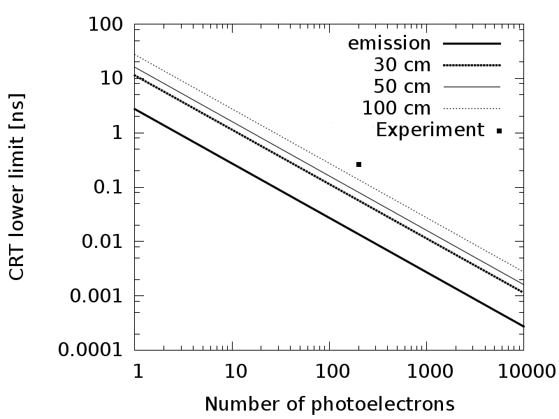
Figure 5: Cramér-Rao lower limit for the time resolution achievable with plastic scintillators calculated as a function of number of registered photons and as a function of the scintillator length assuming cross section of 0.5 cm x 1.9 cm. The meaning of the curves is described in the legend. The square indicates time resolution determined experimentally using a first version of the J-PET prototype with plastic scintillator strips of dimensions 0.5 cm x 1.9 cm x 30 cm (Moskal et al 2014). The result does not include the time spread due to the unknown depth-of-interaction.

In the limit of only one photon the result is quite intuitive since in this case the Cramér-Rao lower bound corresponds to about 3 ns which is approximately in the order of the FWHM of the time distribution of the emitted photons (solid line in Fig. 4) amounting to $\sim$ 3.5 ns. The superimposed square indicates an experimental result obtained for the strip of BC-420 plastic scintillator with the dimensions of 0.5 cm x 1.9 cm x 30 cm read out by Hamamatsu R5320 photomultipliers (Moskal et al 2014). A comparison with the corresponding lower limit implies that there is still room for the substantial improvement of the time resolution. In the next sections we will present a novel solution which allows to improve the time resolution by more than a factor of 1.5.

5 Time resolution as a function of the order statistics for the ideal plastic scintillator

In this section we consider an ideal plastic scintillator detector where all emitted photons are registered by the two ideal photosensors (either left or right) with ideal time resolution and 100% quantum efficiency. It is also assumed that there is no photon absorption and no time spread in the infinitely small plastic scintillator. In Fig. 6 filled symbols show how the coincidence resolving time for first, second and third order statistic changes as a function of the number of emitted photons, and Fig. 7 illustrates how CRT varies as a function of order statistic in the case of 3000 emitted photons. As expected from the shape of the probability density distribution of emitted photons (Fig. 4) the average time difference between emitted photons decreases and hence the time resolution improves with the growing order statistic up to the time when the probability of emission of photons acquires maximum and then time resolution starts to worsen since the average time interval between emitted photons increases.

Having timestamps from all registered photons, in the simplest way we can estimate the hit-time $\Theta$ and time difference $\Delta t$ e.g. as weighted means of corresponding values determined for all ordered statistics:

$$\Theta\equiv\frac{\sum_{i}\frac{\Theta_{(i)}}{\sigma^{2}(\Theta_{(i)})}}{\sum_{i}\frac{1}{\sigma^{2}(\Theta_{(i)})}}=\frac{\sum_{i}\frac{t^{L}_{(i)}/2}{\sigma^{2}(\Theta_{(i)})}}{\sum_{i}\frac{1}{\sigma^{2}(\Theta_{(i)})}}+\frac{\sum_{i}\frac{t^{R}_{(i)}/2}{\sigma^{2}(\Theta_{(i)})}}{\sum_{i}\frac{1}{\sigma^{2}(\Theta_{(i)})}}$$ (9)

$$\Delta t\equiv\frac{\sum_{i}\frac{\Delta t_{(i)}}{\sigma^{2}(\Delta t_{(i)})}}{\sum_{i}\frac{1}{\sigma^{2}(\Delta t_{(i)})}}=\frac{\sum_{i}\frac{t^{L}_{(i)}}{\sigma^{2}(\Delta t_{(i)})}}{\sum_{i}\frac{1}{\sigma^{2}(\Delta t_{(i)})}}-\frac{\sum_{i}\frac{t^{R}_{(i)}}{\sigma^{2}(\Delta t_{(i)})}}{\sum_{i}\frac{1}{\sigma^{2}(\Delta t_{(i)})}}$$ (10)

Figure 6: Coincidence resolving time CRT_(i) as a function of number of emitted photons N simulated assuming the emission time distribution of BC-420 plastic scintillator (solid line in Fig. 4). Filled points denote results for order statistic $i~{}=~{}1$ (circles), $i~{}=~{}2$ (triangles), $i~{}=~{}3$ (squares) and open circles stands for CRT determined based on the weighted time difference $\sigma(\Delta t)$. The result does not include the time spread due to the unknown depth-of-interaction.

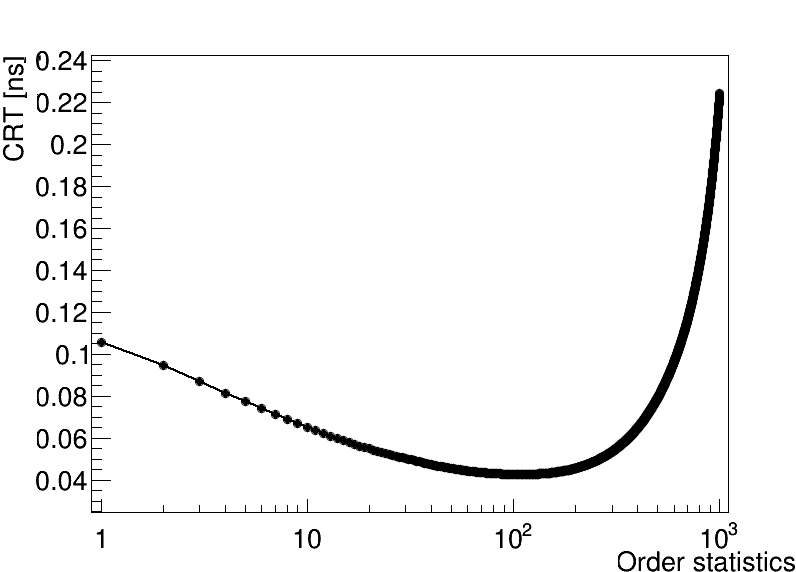
Figure 7: Coincidence resolving time CRT_(i) as a function of order statistic determined based on simulations of 3000 photons using the emission time distribution of BC-420 plastic scintillator (solid line in Fig. 4). The result does not include the time spread due to the unknown depth-of-interaction.

Coincidence resolving time CRT_(i) is presented in Fig. 6 as a function of number of emitted photons assuming the probability density distribution for plastic scintillator BC-420 (solid line in Fig. 4).

These calculations allow us to find out what is the best limit of time resolution for the considered detection systems when the hit-time is estimated as a weighted mean of the registered timestamps. Results shown in Fig. 6 imply that in principle for the energy deposition in the range from 0.2 MeV (2000 photons) to 0.341 MeV (3410 photons) a coincidence resolving time is equal to about CRT = 0.042 ns.

In the following section we will present results of simulations for the solution presently used in the J-PET detector and compare them with the experimental results. Further on simulations with a matrix SiPM readout will be presented and discussed.

6 Time resolution for the single module of the J-PET detector

The realistic simulations of the timestamps registered by the large size scintillator detectors require a proper account for the emission time distribution, photon transport and absorption inside the scintillator, as well as quantum efficiency and transit time spread of photosensors. All these effects have been taken into account as it is described in detail in the Appendix. In this section in order to test the simulation procedures we present results for the plastic scintillator BC-420 with dimensions of 0.5 cm x 1.9 cm x 30 cm read out at two ends by the Hamamatsu R4998 (R5320) photomultipliers. Recent measurements conducted with such detector revealed that about 280 photoelectrons are produced from the emission of about 3410 photons corresponding to the maximum energy deposition of the 0.511 MeV gamma quanta via the Compton effect  (Moskal et al 2014). This is very well reproduced in the simulations as can be inferred from Fig. 8 by a comparison of values at the upper and lower horizontal axes. Fig. 8 shows dependence of the time resolution for the first, second and third order statistic as a function of the number of emitted photons. The result is consistent with the experimental value of CRT equal to about 0.266 ns obtained when determining time at the threshold -50 mV of the leading edge of signals corresponding to the range of number of emitted photons between 2000 and 3410  (Moskal et al 2014). Fig. 8 indicates that in this range the experimental time resolution of 0.266 ns is between the values of time resolutions simulated for the first and third order statistics. This is as expected since predominantly only the first few photoelectrons contribute to the onset of the leading edge of photomultiplier signals. The obtained result shows that in practice the time resolution achievable from the leading edge may be estimated as a mean of resolutions for first and third order statistics. It is also interesting to note that for the discussed detector the best time resolution would be obtained by the measurement of the tenth ordered statistic (Fig. 9).

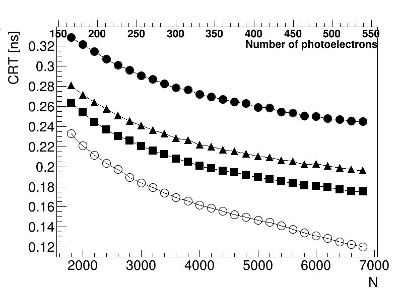
Figure 8: Coincidence resolving time as a function of number of emitted photons N and as a number of photoelectrons simulated for the BC-420 plastic scintillator with dimensions of 0.5 cm x 1.9 cm x 30 cm read out at two ends by the Hamamatsu R4998 (R5320) photomultipliers. Filled points denote results for order statistic $i~{}=~{}1$ (circles), $i~{}=~{}2$ (triangles), $i~{}=~{}3$ (squares) and open circles stand for CRT determined based on the standard deviation of weighted time difference $\sigma(\Delta t)$. The result does not include the time spread due to the unknown depth-of-interaction.

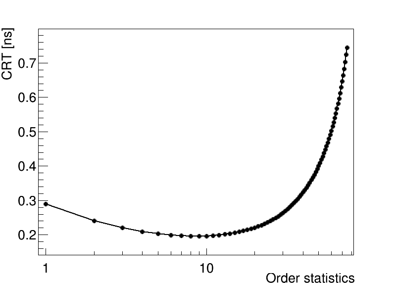
Figure 9: Coincidence resolving time as a function of order statistic i, determined based on simulations of 3000 photons using the emission time distribution of BC-420 plastic scintillator (solid line in Fig. 4) with dimensions of 0.5 cm x 1.9 cm x 30 cm and taking into account a transit time spread of the Hamamatsu R4998 (R5320) photomultipliers. The result does not include the time spread due to the unknown depth-of-interaction.

7 Time resolution for plastic scintillator read out by matrices of silicon photomultipliers

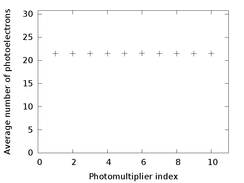
Figure 10: Distribution of average number of registered photons as a function of the ID of the photomultiplier. The simulations were performed for interactions in the center of the scintillator with dimensions of 0.7 cm x 1.9 cm x 30 cm, assuming 3410 photons per interaction, corresponding to the maximum energy deposition of 0.511 MeV gamma quanta via Compton effect.

In the previous sections it was shown that the time resolution may be significantly improved by recording individual timestamps of photons arriving to the scintillator edge. In this section we present simulation of timing properties achievable for the long plastic scintillator strips equipped with readouts at two sides in the form of a matrix of silicon photomultipliers arranged as depicted in Fig. 3. The simulations have been performed assuming properties of the Hamamatsu S12572-100P silicon photomultiplier (Hamamatsu) with photosensitive area of 0.3 cm x 0.3 cm and the width of non-sensitive rim of 0.05 cm, and assuming that the scintillator has dimensions of 0.7 cm x 1.9 cm x 30 cm. A 2 x 5 SIPM matrix (as shown in Fig. 3) enables to cover with the photo-sensitive area about 68% of the end of scintillator with the cross section of 0.7 cm x 1.9 cm. Such matrices of photomultipliers enable to group photons reaching the end of the scintillator into ten subsamples on the left side: ($t^{L}_{1,1},t^{L}_{1,2},...,t^{L}_{1,N1L}$), …, ($t^{L}_{10,1},t^{L}_{10,2},...,t^{L}_{10,N10L}$) and ten subsamples on the right side: ($t^{R}_{1,1},t^{R}_{1,2},...,t^{R}_{1,N1R}$), …, ($t^{R}_{10,1},t^{R}_{10,2},...,t^{R}_{10,N10R}$), where first lower index denotes the ID of SiPM and the second lower index denotes the ID of the photon. Fig. 10 shows that the photons are homogeneously distributed among different photomultipliers and (in the case of the maximum energy deposition by 0.511 MeV gamma quanta) on the average about 22 photons are registered by each SiPM.

Further on, we assume that a timestamp available from a given SiPM corresponds to the time of the fastest photon from the subsample registered by this photomultiplier. Therefore, for each subsample separately, we order timestamps according to ascending time such that: ($t^{L}_{1,(1)}\leq t^{L}_{1,(2)}\leq...\leq t^{L}_{1,(N1L)}$), …, ($t^{L}_{10,(1)}\leq t^{L}_{10,(2)}\leq...\leq t^{L}_{10,(N10L)}$), and analogously for the right side, where indices in brackets indicate timestamps from the ordered subsample. The fastest timestamps in subsamples: $t^{L}_{1,(1)},t^{L}_{2,(1)},...,t^{L}_{10,(1)}$, and $t^{R}_{1,(1)},t^{R}_{2,(1)},...,t^{R}_{10,(1)}$ are considered as timestamps registered by the photomultipliers (hereafter referred to as photomultiplier’s timestamps). Next, for the left and right readout separately, we order the photomultiplier’s timestamps according to ascending time such that: ($t^{L}_{[1]}\leq t^{L}_{[2]}\leq...\leq t^{L}_{[10]}$) and ($t^{R}_{[1]}\leq t^{R}_{[2]}\leq...\leq t^{R}_{[10]}$), where indices in square brackets indicate SiPM timestamps after ordering, and the $t_{[i]}$ element in this set will be hereafter referred to as i-th order SiPM statistic. For each ordered SiPM statistic the interaction time $\Theta_{[i]}$ and the time difference between the signal arrivals to the ends of the scintillator $\Delta t_{[i]}$ are estimated as follows:

$$\Delta t_{[i]}=t^{L}_{[i]}-t^{R}_{[i]},$$ (11)

and

$$\Theta_{[i]}=\frac{t^{L}_{[i]}+t^{R}_{[i]}}{2}+const_{[i]},$$ (12)

where $const_{[i]}$ will be omitted in the further considerations without loss of generality. Finally using information available from all SiPMs we estimate the hit-time $\Theta$ and the time difference $\Delta t$ as the weighted mean of above defined $\Theta_{[i]}$ and $\Delta t_{[i]}$ values, respectively.

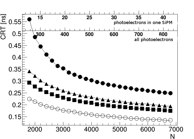
Figure 11: Coincidence resolving time CRT_[i] as a function of number of emitted photons N and as a number of registered photons (photoelectrons) simulated for the BC-420 plastic scintillator with dimensions of 0.7 cm x 1.9 cm x 30 cm read out at two ends by a 2 x 5 matrix of the Hamamatsu S12572-100P silicon photomultipliers. Filled points denote results for the first, second and third SiPM order statistic: $i~{}=~{}1$ (circles), $i~{}=~{}2$ (triangles), $i~{}=~{}3$ (squares) and open circles stand for CRT determined based on the weighted average of all measured $\Delta t_{[i]}$.

Results of the performed simulations are shown in Fig. 11. The number of photoelectrons expected for the maximum energy deposition of 0.511 MeV gamma quanta (N = 3410) is equal to about 440 and is much higher than 280 obtained with the present J-PET prototype. This increase is due to the higher quantum efficiency of S12572-100P silicon photomultipliers with respect to the R4998 (R5320) vacuum tube photomultipliers (see Fig. 17 in the Appendix). Nevertheless, the time resolution for the first SiPM order statistics is worse with respect to the one obtainable with the R4998 (R5320) photomultipliers because of the larger transit time spread of SiPM with respect to R4998 (R5320). However, due to the access to ten SiPM timestamps (available with the 2 x 5 SiPM matrix readout), a coincidence resolving time of CRT $\approx$ 0.180 ns can be achieved when using a weighted mean of the measured SiPM timestamps. This is an average value for the range of interest (from 2000 to 3400 photons). In order to test a dependence of the achievable time resolution on the number of the SiPM in the readout, a systematic simulations were conducted changing the number of SiPM from 2 to 21. Fig. 12 shows CRT obtained for various SiPM configurations. The result indicates that the improvement of resolution saturates with the growing number of photomultipliers, and that the 2 x 5 configurations allowing to read 20 timestamps constitutes an optimal solution and further increase of number of SiPM does not improve the resolution significantly.

As a final result in Fig. 13 a time resolution achievable with vacuum photomultipliers R4998 (R5320) is compared to the resolution achievable with the 2 x 5 SiPM matrix readout for the length of the scintillators from 2.5 cm up to 100 cm. Both results are confronted with the resolution limit simulated for the ideal photosensors allowing for the measurement of each photon reaching the end of the strip. The result presented in the figure indicates that the 2 x 5 SiPM matrix readout can improve the time resolution significantly by about a factor of $1.5$ (up to the length of 50 cm) and that still further significant improvement may be achieved by increasing the quantum efficiency and decreasing the transit time spread with respect to the presently available S12572-100P silicon photomultiplier produced by  Hamamatsu. The comparison was done assuming emission of 2700 photons according to the spectrum of the EJ-230 (BC-420) scintillator. As it was discussed earlier in the text, the number of 2700 photons corresponds to the average amount of photons useful for the positron emission tomography by means of the plastic scintillators. Finally, the obtained results show that the 2 x 5 S12572-100P matrix readout allows to obtain CRT $\approx$ 0.366 ns even for the J-PET constructed with the 100 cm long plastic scintillators.

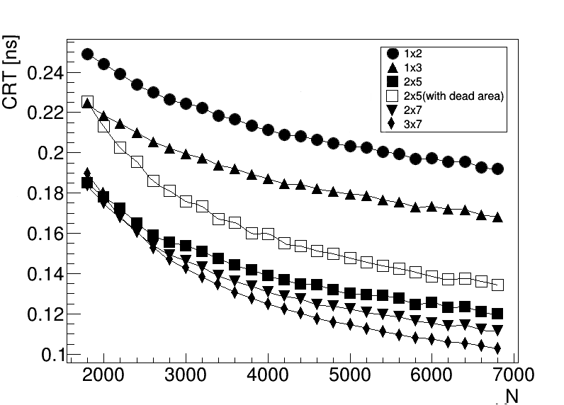
Figure 12: Coincidence resolving time as a function of number of emitted photons N simulated for the BC-420 plastic scintillator with dimensions of 0.7 cm x 1.9 cm x 30 cm. In the simulations it was assumed that the readout consists of photomultipliers characterized by time spread and quantum efficiency the same as the SiPM Hamamatsu S12572-100P but with the dimensions allowing to cover fully the scintillator with the sensitive area with the following readout configurations: 1 x 2 (filled circles), 1 x 3 (filled triangles), 2 x 5 (filled squares), 2 x 7 (filled inverted triangles), and 3 x 7 (filled lozenges). Open squares indicate results for the 2 x 5 configuration taking into account non-sensitive area of the S12572-100P SiPM (the same as in Fig. 11). The result does not include the time spread due to the unknown depth-of-interaction.

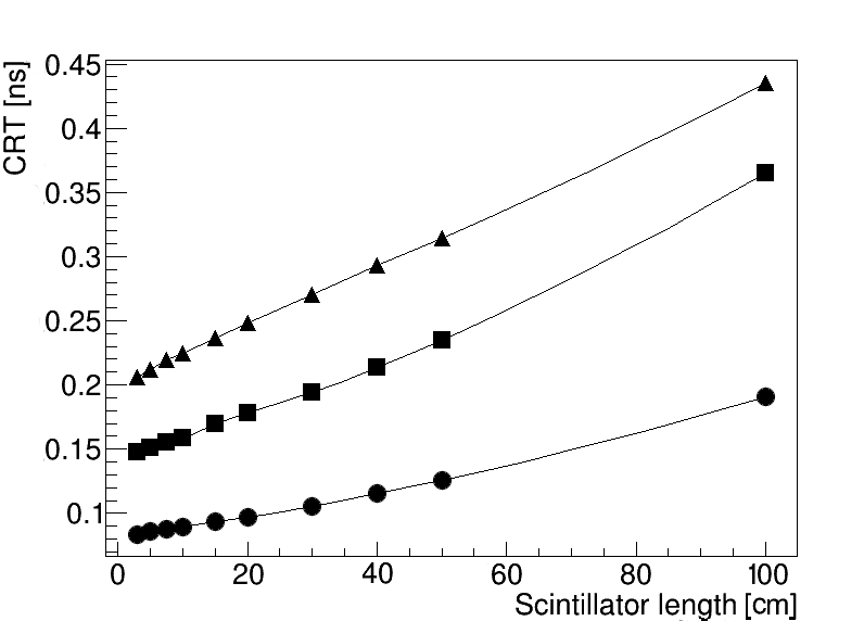
Figure 13: Coincidence resolving time as a function of the scintillator’s length for 2700 emitted photons in the center of the scintillator with the cross section of 0.7 cm x 1.9 cm. (Triangles) A mean value of CRT₍₁₎ and CRT₍₃₎ simulated for the scintillator read out at two ends by the Hamamatsu R4998 (R5320) photomultipliers. (Squares) CRT simulated for the scintillator read out at two ends by the matrix of 2 x 5 S12572-100P photomultipliers. (Circles) CRT determined as a weighted mean from all measured timestamps assuming ideal photosensors with no transit time spread and 100% quantum efficiency and assuming that there is no photon absorption in the scintillator material. The shown values take into account an additional smearing of the time due to the unknown depth of interaction. This can be well approximated by the FWHM equal to about 0.063 ns in the case of the 1.9 cm thick scintillators. The lines are shown to guide the eye.

8 Summary

The realistic simulations based on the Monte-Carlo method were conducted in order to estimate the time resolution achievable with the J-PET tomography scanner built from strips of plastic scintillators (Moskal et al 2011,2014,2015, Raczynski et al 2014,2015). The simulations took into account: (i) emission spectrum of the plastic scintillator BC-420 (EJ-230), (ii) probability density distribution of photon emission times, (iii) transport of photons along the scintillator strip, (iv) absorption of photons in the scintillator material, (v) spectrum of quantum efficiency of photosensors, and (vi) photomultipliers transit time spread. Arrangement of SiPM photosensors in the form of 2 x 5 matrix attached at two ends to the scintillator strip allowed for registering 10 timestamps at each side. These after ordering according to the ascending time were used to estimate the time of interaction as a weighted mean of times registered for each ordered SiPM statistics. Exploitation of information on 10 timestamps at each side improved the time resolution with respect to the present readout based on vacuum tube photomultipliers by about a factor of 1.5 despite the fact that the transit time spread of the considered silicon photosensors S12572-100P ($\sigma$(TTS) = 0.128 ns) is almost two times larger than TTS of photomultipliers R4998 (R5320) ($\sigma$(TTS) = 0.068 ns) used in the present version of the J-PET detector.

For the energy loss in the range from 0.2 MeV to 0.341 MeV (corresponding to the emission of 2000 to 3410 photons), relevant for the positron emission tomography with plastic scintillators, it was shown that with the S12572-100P photosensors arranged into a 2 x 5 matrix at two ends of the scintillator strip the coincidence resolving time changes from CRT $\approx$ 0.170 ns to CRT $\approx$ 0.365 ns when extending an axial field-of-view from 15 cm to 100 cm. This corresponds to the changes of the axial position resolution from 1.4 cm (FWHM) to 3.1 cm (FWHM), respectively. However, as it is shown by solid circles in Fig. 13 there is still room for improving CRT and hence also for improving an axial position resolution by about a factor of two by decreasing the time-jitter of the SiPMs. The results open perspectives for construction of the cost-effective TOF-PET scanner with significantly better TOF resolution and larger field-of-view with respect to the newest TOF-PET modalities characterized by CRT $\approx$ 0.4 ns (Philips,General Electric). In addition, a J-PET scanner built from long strips of plastic scintillators read out by the silicon photosensors, may be combined with the Magnetic Resonance Imaging modality in a way allowing for the simultaneous PET and MRI measurement with the large field-of-view (Moskal 2014b) e.g. by inserting a barrel built of plastic strips into the MRI system.

Finally, it was shown that not only an intrinsic lower bound for the time resolution calculated using the Fisher information and Cramér-Rao inequality, but also more practical limit determined for the time estimated as a mean of all timestamps registered with the ideal photosensor is much lower than the above quoted resolutions. Therefore, there is still room for further improvement of the TOF resolution of the J-PET tomograph which can be achieved anticipating future availability of silicon photosensors with transit-time-spread lower than $\sigma$(TTS) = 0.128 ns of S12572-100P Hamamatsu photomultipliers.

The main purpose of the development of the J-PET system is to find a cost-effective way of the whole body PET imaging. Thus, in order to compare the performance of the J-PET with the presently available LSO based TOF-PET devices, by analogy to references (Conti 2009, Eriksson Conti 2015) we introduce a following formula expressing a figure-of-merit $FOM_{wb}$ relevant for the whole body imaging:

$$FOM_{wb}~{}=\epsilon_{detection}^{2}\times\epsilon_{selection}^{2}\times Acc\ /\ (CRT\times N_{steps}),$$ (13)

where $\epsilon_{detection}$ denotes the detection efficiency of a single 0.511 MeV gamma quantum,

$\epsilon_{selection}$ indicates the selection efficiency of “image-forming” events,

$CRT$ denotes the coincidence resolving time,

$N_{steps}$ indicates number of steps (bed positions) needed to scan a whole body, and

$Acc$ denotes a geometrical acceptance.

In the first order of approximation we may assume that $N_{steps}$ is inversely proportional to the AFOV, and that the term $\epsilon_{detection}^{2}\times Acc$ is proportional to the $\int_{\theta_{min}}^{\theta_{max}}(\epsilon_{0detection}/\sin\!\theta)^{2}\sin\!\theta d\theta$, where $\theta$ denotes the angle between the direction of the gamma quanta and the main axis of the tomograph; the term $\epsilon_{0detection}/\sin\!\theta$ accounts for the changes of the detection efficiency as a function of the $\theta$ angle, with $\epsilon_{0detection}$ denoting detection efficiency when gamma quantum crosses the detector perpendicularly to its surface; $\sin\!\theta d\theta$ stands for the angular dependence of the differential element of the solid angle, and $\theta_{min}$ to $\theta_{max}$ determines the range of angular acceptance of the tomograph. The above assumptions yield:

$$FOM_{wb}~{}=\int_{\theta_{min}}^{\theta_{max}}(\epsilon_{0detection}/\sin\!\theta)^{2}\sin\!\theta d\theta\times AFOV\ /\ CRT.$$ (14)

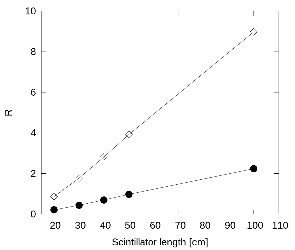
Figure 14: A ratio of figure of merits for the whole body imaging with J-PET and LSO based PET detectors defined as R(AFOV-J-PET) = $FOM_{wb}$(AFOV-J-PET) / $FOM_{wb}$(LSO with AFOV=20cm). Horizontal axis of the figure refers to the length of the J-PET detector. The length of the LSO scanner was fixed to 20 cm, and the diameter of the scanners was fixed to 80 cm. Full dots indicate result determined for a single J-PET layer ($N_{layers}$ = 1), and open squares indicate result for J-PET with two layers ($N_{layers}$ = 2). For small number of layers, the $\epsilon_{detection}$ of the J-PET detector is approximately proportional to $N_{layers}$. The presented result was obtained under assumptions that CRT of the LSO based detectors is equal to 0.4 ns and that CRT values of the J-PET corresponds to the results of this article shown by full squares in Fig. 13. Calculations of $FOM_{wb}$ of the J-PET were performed assuming a threshold of 0.2 MeV. The lines connecting points are shown to guide the eye, whereas the horizontal solid line indicates R = 1.

Fig. 14 shows the ratio $R$ of $FOM_{wb}$ of the J-PET and LSO based PET detectors defined as: R(AFOV-J-PET) = $FOM_{wb}$(AFOV-J-PET)/$FOM_{wb}$(LSO with AFOV = 20 cm). The shown ratio is determined for a fixed AFOV = 20 cm of the LSO based PET, but varying the AFOV of the J-PET detector. Full dots indicate result determined for a single J-PET layer ($N_{layers}$ = 1), and open squares indicate result for J-PET with two layers ($N_{layers}$ = 2). The results shown in Fig. 14 were obtained assuming a 2 cm radial thickness of the detection layers and taking into account that linear attenuation coefficients of 0.511 MeV gamma quanta are equal to $\mu_{LSO}~{}=~{}0.87~{}cm^{-1}$ (Mechler 2000) and $\mu_{plastic}~{}=~{}0.098~{}cm^{-1}$ (Saint Gobain Crystals). Furthermore it was assumed that (i) CRT of LSO based scanners is equal to 0.4 ns as achieved recently by manufacturers Philips (Philips) and General Electric (General Electric), and that (ii) $\epsilon_{selection}$ for LSO is equal to 0.32, which is a fraction of the photoelectric effect in the case of the LSO crystals [Humm2003], and that (iii) $\epsilon_{selection}$ of the J-PET is equal to 0.44 which corresponds to the fraction of events with energy deposition larger than 0.2 MeV in the case of plastic scintillators. Fig. 14 indicates that in order to compensate for the lower efficiency of plastic scintillators and thus to obtain $FOM_{wb}$ of the J-PET comparable to the LSO based scanners with AFOV = 20 cm it is required to use either two detection layers or to increase the J-PET AFOV to about 50 cm. Certainly the $FOM_{wb}$ of the LSO based PET would also grow approximately as square of AFOV but at the same time the cost of such PET detector would increase almost linearly proportional to AFOV, whereas the cost of the J-PET does not increase significantly when increasing the AFOV.

The relative ease of the cost effective increase of the axial field-of-view makes the J-PET tomograph competitive with respect to the current commercial PET scanners as regards sensitivity and time resolution, yet this is achieved at the expense of the significant reduction of the axial spatial resolution. Finally, it is worth to stress that the J-PET with a long diagnostic chamber opens unique perspectives for simultaneous whole-body metabolic imaging not accessible with the presently available PET/CT modalities.

9 Acknowledgements

We acknowledge technical and administrative support of T. Gucwa-Rys, A. Heczko, M. Kajetanowicz, G. Konopka-Cupiał, W. Migdał, and the financial support by The Polish National Center for Research and Development through grant INNOTECH-K1/IN1/64/159174/NCBR/12, the Foundation for Polish Science through MPD programme, the EU and MSHE Grant No. POIG.02.03.00-161 00-013/09, Doctus - the Lesser Poland PhD Scholarship Fund, and Marian Smoluchowski Krakow Research Consortium ”Matter-Energy-Future”.

10 References

3M Optical Systems, www.3M.com/Vikuiti

Baszak J 2014 Hamamatsu, private communication.

Bettinardi V et al 2011 Physical Performance of the new hybrid PET-CT Discovery-690 FWH-TOF=544ps Med. Phys. 38 5394-5411

Conti M 2009 State of the art and challenges of time-of-flight PET Phys. Med. 25 1-11

Conti M 2011 Focus on time-of-flight PET: the benefits of improved time resolution Eur. J. Nucl. Med. Mol. Imaging 38 1147-1157

Conti M, Eriksson L, Rothfuss H, Melcher C L 2009 Comparison of Fast Scintillators With TOF PET Potential IEEE Trans. Nucl. Sci. 56 926-933

DeGroot M H 1986 Probability and Statistics Addison-Weslay 420-6

Eljen Technology, www.eljentechnology.com

Eriksson L and Conti M 2015 Randoms and TOF gain revisited Phys. Med. Biol. 60 1613-1623

Fishburn M W and Charbon E 2010 System Tradeoffs in Gamma-Ray Detection Utilizing SPAD Arrays and Scintillators IEEE Trans. Nucl. Sci. 57 2549-2557

General Electric, http://www3.gehealthcare.com/en/products/categories/magnetic_resonance_imaging/signa_pet-mr

Hamamatsu, www.hamamatsu.com

Humm J L, Rosenfeld A, Del Guerra A 2003 From PET detectors to PET scanners Eur. J. Nucl. Med. Mol. Imaging 30 1574-1597

Karp J S et al 2008 Benefit of Time-of-Flight in PET: Experimental and Clinical Results J. Nucl. Med. 49 462-470

Korcyl G et al 2014 Trigger-less and reconfigurable data acquisition system for positron emission tomography Bio-Algorithms and Med-Systems 10 37-40

Kowalski P et al 2015 Multiple scattering and accidental coincidences in the J-PET detector simulated using GATE package Acta Phys. Pol. A 127 1505-1512 [arXiv:1502.04532 [physics.ins-det]].

Kuhn A et al 2006 Performance assessment of pixelated LaBr3 detector modules for time-of-flight PET IEEE Trans. Nucl. Sci. 53 1090-1095

Lecoq P, Auffray E, Knapitsch A 2013 How Photonic Crystals Can Improve the Timing Resolution of Scintillators IEEE Trans. Nucl. Sci. 60 1653-1657

Mechler C L 2000 Scintillation Crystals for PET, J. Nucl. Med. 41 1051-1055

Meijlink J R et al 2011 First Measurement of Scintillation Photon Arrival Statistics Usign a High-Granularity Solid-State Photosensor Enabling Time-Stamping of up to 20,480 Single Photons Proc. IEEE Nuclear Science Symposium (NSS/MIC). 2254-2257

Moses W W, Derenzo S E 1999 Prospects for Time-of-Flight PET using LSO Scintillator IEEE Trans. Nucl. Sci. 46 474-478

Moses W W 2003 Time of Flight in PET Revisited IEEE Trans. Nucl. Sci. 50 1325-1330

Moskal P et al 2011 Novel detector systems for the Positron Emission Tomoraphy Bio-Algorithms and Med-Systems 7 73-78; [arXiv:1305.5187 [physics.med-ph]].

Moskal P et al 2012 TOF-PET detector concept based on organic scintillators Nuclear Medicine Review 15 C81-C84; [arXiv:1305.5559 [physics.ins-det]].

Moskal P et al 2014 Test of a single module of the J-PET scanner based on plastic scintillators Nucl. Instrum. Methods Phys. Res. A 764 317-321; [arXiv:1407.7395 [physics.ins-det]].

Moskal P 2014b A hybrid TOF-PET/MRI tomograph Patent Application PCT/EP2014/068373 WO2015028603 A1

Moskal P et al 2015 A novel method for the line-of-response and time-of-flight reconstruction in TOF-PET detectors based on a library of synchronized model signals Nucl. Instrum. Methods Phys. Res. A 775 54-62; [arXiv:1412.6963 [physics.ins-det]].

Moszynski M and Bengtson B 1977 Light pulse shapes from plastic scintillators Nucl. Instrum. Methods 142 417-434

Moszynski M and Bengtson B 1979 Status of timing with plastic scintillation detectors Nucl. Instrum. Methods 158 1-31

Moszynski M, Szczesniak T 2011 Optimization of Detectors for Time-of-Flight PET Acta Phys. Pol. B. Proc. Supp. 4 59-64

Nickles R J, Meyer H O 1978 Design of a three-dimensional positron camera for nuclear medicine Phys. Med. Biol. 23 686-695

Palka M et al 2014 A novel method based solely on FPGA units enabling measurement of time and charge of analog signals in Positron Emission Tomography Bio-Algorithms and Med-Systems 10 41-45; [arXiv:1311.6127 [physics.ins-det]].

Philips, http://www.philips.co.uk/healthcare/product/HC882446/vereos-digital-pet-ct

Raczyński L et al 2014 Novel method for hit-position reconstruction using voltage signals in plastic scintillators and its application to Positron Emission Tomography Nucl. Instrum. Methods Phys. Res. A 764 186-192; [arXiv:1407.8293 [physics.ins-det]].

Raczyński L et al 2015 Compressive Sensing of Signals Generated in Plastic Scintillators in a Novel J-PET Instrument Nucl. Instrum. Methods Phys. Res. A 786 105-112; [arXiv:1503.05188 [physics.ins-det]].

Saint Gobain Crystals www.crystals.saint-gobain.com

Seifert S, van Dam H T, Schaart D R 2012 The lower bound on the timing resolution of scintillation detectors Phys. Med. Biol. 57 1797-1814

Seifert S,van Dam H T, Vinke R, Dendooven P, Lohner H, Beekman F J, Schaart D R 2012 A Comprehensive Model to Predict the Timing Resolution of SiPM-Based Scintillation Detectors: Theory and Experimental Validation IEEE Trans. Nucl. Sci. 59 190-204

Schaart R D et al 2009 A novel, SiPM-array-based, monolithic scintillator detector for PET Phys. Med. Biol. 54 3501-3512

Schaart R D et al 2010 LaBr3:Ce and SiPMs for TOF PET: achieving 100ps coincidence resolving time. Phys. Med. Biol. 55 N179-N189

Senchyshyn V et al 2006 Accounting for self-absorption in calculation of light collection in plastic scintillators Nucl. Instrum. Methods Phys. Res. A 566 286-293

Spanoudaki V Ch and Levin C S 2011 Investigating the temporal resolution limits of scintillation detection from pixellated elements: comparison between experiment and simulations Phys. Med. Biol. 56 735-756

Surti S et al 2007 Performance of Philips Gemini TF PET/CT Scanner with Special Consideration for Its Time-of-Flight Imaging Capabilities J. Nucl. Med. 48 471-480

Szymański K et al 2014 Simulations of gamma quanta scattering in a single module of the J-PET detector Bio-Algorithms and Med-Systems 10 71-77

Townsend D W 2004 Physical Principles and Technology of Clinical PET Imaging Ann. Acad. Med. Singapore 33 133-145

APPENDIX: Simulation of photon transport in cuboidal scintillator strips

In a long scintillator strip, a photon on its way from the emission point to the photomultiplier may undergo many internal reflections whose number strongly depends on the scintillator size and the photon emission angle. However, the space reflection symmetries of the cuboidal shapes, which are considered in this article, enables a significant simplification of the photon transport algorithm, without following photon propagation in a typical manner. In our simulations for each emitted photon the initial direction of its flight is obtained in polar coordinate system as two uniformly distributed random values of $cos\theta$ and $\phi$, where $\theta$ is the angle between flight direction and $z$-axis and $\phi$ is the azimuthal angle as defined in standard spherical coordinate system. The coordinate system is defined in Fig. 3 where the $z$-axis is directed along the longest axis of the scintillator strip. The components of photon flight direction vector can be expressed as follows:

$$\vec{dir}=[sin\theta cos\phi,~{}sin\theta sin\phi,~{}cos\theta]$$ (15)

The number of reflections from the side surfaces that are normal to $x$ or $y$-axis are calculated using the projection of the flight-direction vector to $y$-$z$ or $x$-$z$-plane, respectively:

$$tg\theta_{x}=\frac{dir_{x}}{dir_{z}};~{}tg\theta_{y}=\frac{dir_{y}}{dir_{z}},$$ (16)

where $\theta_{x}$ is the angle between $\vec{dir}$ projection on $x$-$z$-plane and $z$-axis and $\theta_{y}$ is the same for projection on $y$-$z$-plane.

Taking into account the fact that each reflection changes only the sign of respective component of $\vec{dir}$ we can assume that the reflection angle is not changed for each pair of side surfaces during the whole photon flight. So we need to obtain two values of reflection angle: one for side surfaces normal to $x$-axis and one for ones normal to $y$-axis. Knowing that $|\vec{dir}|=1$ and that these are the angles between photon flight direction and the normal vectors for respective side surfaces ($x$ and $y$ axes) we obtain:

$$cos\alpha_{x}=dir_{x};~{}cos\alpha_{y}=dir_{y},$$ (17)

where $\alpha_{x}$ and $\alpha_{y}$ are the reflection angles for side surfaces normal to respective axis. Then the probability of photon’s reaching the photomultiplier can be calculated using a following formula:

$$P_{reach}=P_{refl}(sin\alpha_{x})^{n_{x}}P_{refl}(sin\alpha_{y})^{n_{y}},$$ (18)

where $n_{x}$ and $n_{y}$ denote the respective numbers of reflections. The dependence $P_{refl}(sin\alpha)$ is obtained from Fresnel equations and is shown in Fig. 15.

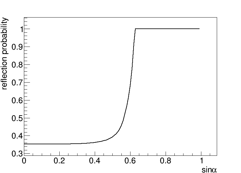
Figure 15: The dependence of reflection probability on sinus of the reflection angle $\alpha$.

Further factors that influence the photon registration probability are absorption in the scintillator material, losses at surface imperfections, and the photomultiplier’s quantum efficiency. In current algorithm of simulation the following formula for photon registration probability has been used

$$P_{reg}=P_{reach}~{}\epsilon(\lambda)~{}e^{-{\mu_{eff}(\lambda)}~{}\frac{\Delta L}{cos\theta}}$$ (19)

where $P_{reach}$ denotes the probability from formula (18), $\lambda$ denotes the photon’s wavelength, $\epsilon(\lambda)$ stands for the photomultiplier’s quantum efficiency and $\mu_{eff}(\lambda)$ is the effective absorption coefficient for the scintillator material. The latter, shown by thick solid line in Fig. 16, accounts effectively for the absorption of photons on the way to photomultipliers and was determined by scaling the absorption coefficient of pure polystyrene (Senchyshyn et al 2006) to the experimental results obtained with the single detection unit of the J-PET detector  (Kowalski et al 2015). The scaling factor accounts effectively for the absorption due to the primary and secondary admixture in the scintillator material, imperfections of surfaces and reflectivity of the foil (Kowalski et al 2015). It was determined by the comparison of simulations with experimental results obtained for the EJ-230 plastic scintillator with dimensions of 0.5 cm x 1.9 cm x 30 cm (Kowalski et al 2015).

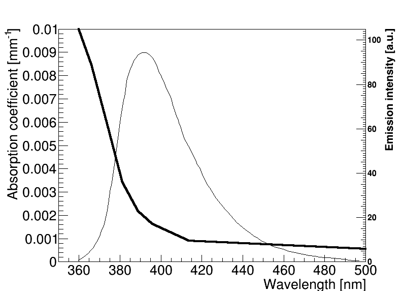
Figure 16: (Thick line) The dependence of scintillator’s absorption coefficient $\mu_{eff}$ on photon’s wavelength. The effective coefficient $\mu_{eff}$ was determined by scaling the absorption coefficient of the pure polystyrene (Senchyshyn et al 2006) by factor of 1.8 (Kowalski et al 2015). (Thin line) Emission spectrum of the BC-420 plastic scintillator (Saint Gobain Crystals). The left axis denotes absorption coefficient and right axis denotes the emission intensity.

Photomultipliers quantum efficiencies that were used in current calculations are shown in Fig. 17.

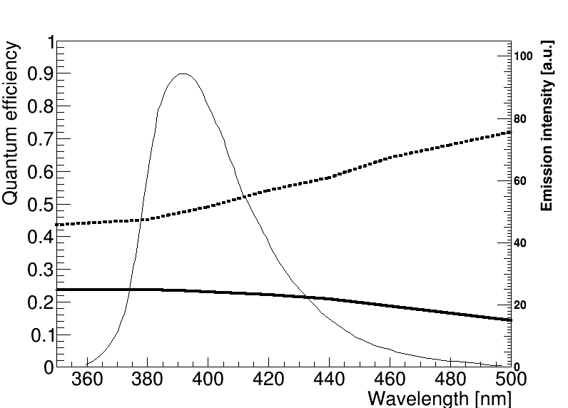
Figure 17: Quantum efficiency as a function of photon’s wavelength for Hamamatsu R4998 (R5320) photomultiplier (Baszak 2014) (solid line) and Hamamatsu silicon S12572-100P photomultiplier (dashed line). A superimposed thin solid line denotes emission spectrum of the Saint Gobain BC-420 plastic scintillator. The left axis denotes quantum efficiency and right axis denotes the emission intensity.

The time of arrival $t_{i}^{arrival}$ of $i$th photon at the photomultiplier (or in general the time of passing a given distance ${\Delta L}$ along the scintillator) may be expressed as:

$$t_{i}^{arrival}=t_{i}^{e}+\frac{\Delta L}{\frac{c}{n}cos\theta},$$ (20)

where $t_{i}^{e}$ is the emission time of $i$th photon, $\Delta L$ denotes the distance between the emission point and the photomultiplier, $c$ denotes the speed of light and $n$ stands for scintillator’s refractive index (the value of $n=1.58$ was used) (Saint Gobain Crystals).

Finally, the timestamp $t_{i}$ is simulated by smearing the time $t_{i}^{arrival}$ taking into account the transition time spread of the photosensors:

$$t_{i}=t_{i}^{arrival}+RG(t_{offset},\sigma_{t}),$$ (21)

where $RG(0,\sigma)$ is value generated randomly according to the Gauss distribution with the mean at $t_{offset}$, and with standard deviation $\sigma_{t}$ equal to the standard deviation of time spread of a given photomultiplier. For simulations referred to in this paper as done with ”ideal photomultiplier” $\sigma_{t}=0$. Otherwise for Hamamatsu R4998 (R5320) photomultiplier $\sigma_{t}=0.068~{}ns$ Hamamatsu and for silicon photomultiplier S12572-100P $\sigma=0.128~{}ns$ Hamamatsu. The parameter $t_{offset}$ accounts for all constant electronic time delays and its value does not influence the time resolution. Therefore, for simplicity, but without loss of generality, it is set to zero.