Instability in electromagnetically driven flows
Part I

Abstract

The MHD flow driven by a travelling magnetic field (TMF) in an annular channel is investigated numerically. For sufficiently large magnetic Reynolds number $Rm$, or if a large enough pressure gradient is externally applied, the system undergoes an instability in which the flow rate in the channel dramatically drops from synchronism with the wave to much smaller velocities. This transition takes the form of a saddle-node bifurcation for the time-averaged quantities. In this first paper, we characterize the bifurcation, and study the stability of the flow as a function of several parameters. We show that the bifurcation of the flow involves a bistability between Poiseuille-like and Hartman-like regimes, and relies on magnetic flux expulsion. Based on this observation, new predictions are made for the occurrence of this stalling instability.

I Introduction

The driving of an electrically conducting fluid by an electromagnetic force due to a travelling magnetic field can yield significantly more complex behaviors than its solid equivalent, the asynchronous motor. In particular, the many degrees of freedom of the fluid and the presence of magnetohydrodynamic boundary layers strongly affects the behavior of the system, and several questions concerning the stability of such flows remain unsolved.

These questions become of primary interest in many industrial situations. For instance, Electromagnetic Linear Induction Pumps (EMPs) are largely used in secondary cooling systems of fast breeder reactors, mainly because of the ease of maintenance due to the absence of bearings, seals and moving parts. In these EMPs, the conducting fluid is generally driven in a cylindrical annular channel by means of a travelling magnetic field imposed by external coils. In such induction pumps, electrical currents in the liquid are induced by the variation of the magnetic flux of the wave, rather than injected through electrodes, as in conduction pumps Stelzer15 . In this perspective, several experimental studies of annular EMPs have been conducted Andreev78 ; Kliman79 ; Ota04 , in which the main characteristics of such pumps under large values of MHD interaction parameters have been described.

It is expected that as these pumps become large enough, a magnetohydrodynamic instability arises, yielding significant decrease in the developed flow rate. Gailitis and Lielausis Galaitis76 first provided a theoretical analysis of this problem and proposed a magnetohydrodynamic criterion for the occurrence of the instability in such pumps. Based on the large aspect ratio $r_{inner}/r_{outer}$ generally used in experimental or industrial pumps, this theoretical description of electromagnetically driven flows relies on the assumption that the velocity field is invariant in the radial direction. According to this model, the instability occurs above some critical magnetic Reynolds number $Rm_{c}$ and takes the form of an inhomogeneity in the azimuthal direction. Several experimental studies Kirillov80 ; Araseki04 have shown that when $Rm>Rm_{c}$, a low frequency pulsation in the pressure and the flow rate is indeed observed, strongly reducing the efficiency of the pump. More recently, significant progress has been done on the understanding of these electromagnetically driven flows. First, it has been shown through numerical and experimental studies Araseki00 that even at low $Rm$, the efficiency of such pumps is affected by an amplification of the electromagnetic forcing, which takes the form of a strong pulsation at double supply frequency (DSF). Second, it has been confirmed that at large $Rm$, an azimuthal non-uniformity of the applied magnetic field or of the sodium inlet velocity can create vortices in the annular gap Araseki04 . In both cases (large and low $Rm$), some solutions have been proposed to inhibit the occurrence of these perturbations, but this generally leads to a strong loss of efficiency of the pump. One purpose of the present article is to provide a study of the physical mechanism by which the flow becomes unstable in such systems in order to suggest new types of solutions for suppressing the occurrences of the perturbations mentioned above.

In the present work, we numerically investigate a simple configuration aiming to reproduce an electromagnetic pump. In the first part of the article, we report calculations in the laminar regime and describe the instability arising when the magnetic Reynolds number is large enough. After emphasizing the physical mechanism by which the instability occurs, we propose a new criterion for the instability threshold. In the second part of the paper, a new type of instability is reported in 2D calculations performed at large Reynolds numbers. We show how large scale vortices are created in the flow due to induction effect, but only when the flow is turbulent enough. We show that this instability is related to end-effects and can be understood in the framework of a simple model. Finally, we discuss these results in the perspective of large scale experimental electromagnetic pumps and propose a configuration inhibiting these type of destabilization.

II Theoretical description of an ideal cylindrical machine

Before describing our numerical results, it may be useful to briefly recall the equations obtained in the framework of the traditional theory of induction-type cylindrical magnetohydrodynamics (MHD) machines.

Figure 1: Schematic view of a typical electromagnetic pump

A schematic view of a typical electromagnetic pump is shown in Fig. 1. In general, the liquid metal flows along an annular channel confined by two concentric cylinders. Some ferromagnetic cores can be placed on the inner side of the channel, in order to reinforce the radial component of the magnetic field created by a three-phase winding of electrical currents imposed on the outer side of the channel.

The governing equations are the magnetohydrodynamics equations, i.e. the Navier-Stokes equation coupled to the induction equation

$$\rho\frac{\partial\boldsymbol{u}}{\partial t}+\rho\left(\boldsymbol{u}\cdot\boldsymbol{\nabla}\right)\boldsymbol{u}=-\boldsymbol{\nabla}P+\rho\nu\boldsymbol{\nabla}^{2}\boldsymbol{u}+\boldsymbol{j}\boldsymbol{\times}\boldsymbol{B}\ ,$$ (1)

$$\frac{\partial\boldsymbol{B}}{\partial t}=\boldsymbol{\nabla}\boldsymbol{\times}\left(\boldsymbol{u}\boldsymbol{\times}\boldsymbol{B}\right)+\frac{1}{\mu_{0}\sigma}\boldsymbol{\nabla}^{2}\boldsymbol{B}\ .$$ (2)

where $\rho$ is the density, $\nu$ is the kinematic viscosity, $\sigma$, is the electrical conductivity, $\mu_{0}$ is the magnetic permeability, $\nu$ is the fluid velocity, $\boldsymbol{B}$ is the magnetic field, and $\boldsymbol{j}=\mu_{0}^{-1}\boldsymbol{\nabla}\boldsymbol{\times}\boldsymbol{B}$ is the electrical current density.

In several references, electromagnetic pumps are modeled through a modification of the above classical MHD equations solved in the liquid domain, for instance by adding a source term in equation 2 which represents the effect of the external coils. As this approach is generally safe when modeling an external homogeneous and stationary magnetic field, the interpretation of such a modification is more complicated when dealing with a travelling wave, since it could be equivalent to add some unphysical source term to Maxwell’s equations. For instance, some authors incorrectly use a modified Ohm’s law in which a source term $J_{0}$ is added, and interpret $B$ in equation 2 as an ’induced’ magnetic field.

Another approach is to decompose the total magnetic field $B$ in the channel between two parts $B=B_{0}+b$, where $B_{0}$ is the magnetic field that would be created inside the annular gap in absence of conducting media, by any external sources (coils, permanent magnets, etc). $b$ can therefore be regarded as the magnetic field generated by the presence of induced currents within the conducting fluid.

In the present article, we chose to use a third approach relying on the modification of boundary conditions only, which ensures no modification of Maxwell’s equations whereas keeping a relatively simple modelisation, without dealing with the external domain.

On the cylinders, we consider high permeability boundary conditions, for which the magnetic field is forced to be normal to each boundary. This models the presence of ferromagnetic cores generally found in electromagnetic pumps. In addition, the presence of azimuthal coils is modeled by an azimuthal electrical current $J_{s}$ imposed on the outer cylinder, such that the boundary conditions on $r_{o}$ become:

$$\left({\bf B_{2}}-{\bf B_{1}}\right)\cdot{\bf e_{r}} = 0$$ (3)

$${\bf e_{r}}\times\left(\frac{{\bf B_{2}}}{\mu_{2}}-\frac{{\bf B_{1}}}{\mu_{1}}\right) = J_{s}{\bf e_{\phi}}$$ (4)

where the subscripts $1$ and $2$ respectively refers to the liquid metal (inside) and the external boundary (outside). In the limit of an external ferromagnetic boundary ($\mu_{1}/\mu_{2}\ll 1$), in which the magnetic permeability $\mu_{2}$ of the boundary is much larger than the permeability of the fluid $\mu_{1}$, this reduces to

$$B_{\phi}(r_{o})=0\hskip 5.69054pt \hskip 5.69054ptB_{z}(r_{o})=\mu_{1}J_{s}$$ , (5)

$$B_{\phi}(r_{i})=0\hskip 5.69054pt \hskip 5.69054ptB_{z}(r_{i})=0$$ , (6)

The surface current $J_{s}$ is imposed :

$$J_{s}=J_{0}e^{i\left(kz-\omega t\right)}$$ (7)

where $J_{0}$ is the complex amplitude of the applied current. Therefore, $\omega$ and $k=2\pi/\lambda$ are respectively the pulsation and the wavenumber of the wave.

When considering an axisymmetric problem, one can introduce the vector potential $A(r,z,t){\bf e_{\phi}}$ defined by ${\bf B}={\bf\nabla\times A}$, such that the induction equation becomes :

$$\frac{\partial A}{\partial t}+V\frac{\partial A}{\partial z}=\frac{1}{\mu_{0}\sigma}\left(\frac{\partial^{2}A}{\partial^{2}r}+\frac{\partial^{2}A}{\partial^{2}z}\right)$$ (8)

where the small-gap limit has been used. Here, ${\bf V}=V{\bf e_{z}}$ is the velocity of the fluid, and in the following theoretical description will be assumed to be only in the $z$-direction, and completely homogeneous over the section of the annular gap. Note that this homogeneous velocity of the fluid over the entire cross-section constitutes one of the most drastic assumption of the present derivation, and clearly contradicts the no-slip boundary conditions used in our simulations. Due to the sinusoidal current applied on the outer boundary, we assume that the vector potential is of the form $A(r,z,t)=\tilde{A}(r,t)e^{ikz}$, leading to the equation:

$$\partial_{t}\tilde{A}+ik\tilde{A}V=\eta(-k^{2}\tilde{A}+\partial_{rr}\tilde{A})$$ (9)

where $\eta=1/\mu_{0}\sigma$ is the magnetic diffusivity. This equation can be solved by using boundary conditions (5)-(6) and gives the radial structure of the magnetic field across the gap for a given velocity $V$. Here, we will rather integrate this equation along the radial direction in the gap $d=r_{o}-r_{i}$. By defining the r-averaged vector potential $\Phi=\displaystyle\frac{1}{d}\int_{r_{i}}^{r_{o}}\tilde{A}\,\mathrm{d}r$, eq. (9) becomes:

$$\partial_{t}\Phi=-(ikV+\eta k^{2})\Phi+\frac{J_{0}}{d\sigma}e^{-i\omega t}$$ (10)

where the boundary conditions $\partial_{r}\tilde{A}|_{r_{o}}=J_{0}e^{-i\omega t}$ and $\partial_{r}\tilde{A}|_{r_{i}}=0$ have been used.

Similarly to $\Phi$, we can compute the large scale r-averaged induced current:

$$J(z,t)=\frac{1}{d}\left(\int_{r_{i}}^{r_{o}}j(r,z,t)\,\mathrm{d}r-J_{s}\right)=\left(\frac{k^{2}}{\mu}\Phi-\frac{2J_{0}}{d}e^{-i\omega t}\right)e^{ikz}$$ (11)

The total Lorentz force (averaged in the axial direction) acting on the fluid is then given by:

$$F_{B}=\frac{1}{2}\Re\{{\bf J^{*}}\times{\bf B}\}=\Re\{i\frac{kJ_{0}}{d}\Phi e^{i\omega t}\}$$ (12)

Here, both $J$ and $B$ in the above expression are large scale quantities averaged in the radial direction, implying that r-dependent perturbations are considered small compared to the mean values. Since the Lorentz force is quadratic in the magnetic field, it generally produces a forcing on the flow with a component at a pulsation $2\omega$, which is twice the one of the applied current. At small magnetic Reynolds number, this component can be amplified and leads to the so-called Double Supply Frequency (DSF) pulsation observed in some experimental pumps Araseki00 . Note that this component is filtered out in the present model, since only averaged quantities are considered.

In addition to this electromagnetic force, the flow undergoes a friction force due to the viscosity. If the Darcy-Weisbach equation for a pipe flow in the limit of purely hydrodynamical flows is used to evaluate the pressure loss due to friction, Navier-Stokes equations reduce to:

$$\rho\frac{\partial V}{\partial t}=K+F_{B}-\frac{\lambda\rho}{d}V^{2}\text{sign}(V)$$ (13)

where $\rho$ is the density, $K=-\partial_{z}p$ is some imposed axial pressure gradient and $\lambda$ is a friction parameter (supposed independent of $Re$ for simplicity).

Finally, by taking a timescale $t_{0}=1/\omega$, a velocity scale $v_{0}=\omega/k=c$ and a scale of magnetic field $B_{0}=\mu J_{0}$, and writing eq. (10) and (13) in dimensionless form, we get the following system:

$$R\dot{\Phi} = -(1+iRq)\Phi+e^{-iT}$$ (14)

$$\dot{q} = -\gamma q^{2}\text{sign}(q)-\frac{H^{2}\gamma}{R}\Re\{i\Phi e^{iT}\}+\kappa$$ (15)

with $\kappa=\Delta P/\rho c^{2}$ and $\gamma=\lambda/k\delta$. The two dimensionless numbers $R=\omega/\eta k^{2}$ and $H=\mu_{0}J_{0}^{2}/(\rho\lambda\omega\eta kd))$ can be regarded as respectively a magnetic Reynolds number and an Hartmann number based on the wave characteristics. $q=v/c$ is the normalized velocity of the fluid and $T$ the dimensionless time. Equations (14) and (15) therefore provide a simple dynamical system describing the evolution of space averaged fields in the electromagnetic pump.

Let us now search for a pure travelling wave solution, for which $\dot{q}=0$ and $\Phi=\Phi_{0}e^{-iT}$. In this case, our system of equations simply reduces to:

$$\Phi_{0}=\frac{1}{1-iR(1-q)}$$ (16)

$$\kappa=H^{2}\frac{1-q}{1+R^{2}(1-q)^{2}}-q^{2}\text{sign}(q)=F(q)$$ (17)

The last equation is the so-called PQ-characteristic of the pump, in which the applied pressure gradient balances the Lorentz force and the viscous force. It is identical to the expression found by Galaitis76 .

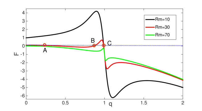
Figure 2: Theoretical characteristic curve F(q) for $Ha=10$, and $R=10$ (black curve), $R=30$ (red) and $R=70$ (green).

Due to the assumption of an homogeneous velocity, expression (17) is very similar to the equation predicting the stalling of an asynchronous motor, and is sometimes referred as the PQ (for Pressure P and Flow rate Q) characteristic of the pump. Figure 2 helps to understand the typical transitions prone to appear in such systems. At large $H$ and moderate $R$, the viscous dissipation is relatively small compared to the magnetic force, and the system operates near $q=1$, where $F=0$ (for instance the black curve in fig. 2). As $R$ is increased (red curve), one can see that $F(q)$ intersects the line $F=0$ in three locations corresponding to three different fixed points ($A$, $B$ and $C$). Two of these solutions are stable equilibria (both points $A$ and $C$ lie on the descending parts of the curve) whereas the third one is unstable ($B$ is located on the ascending part). A further increase of $R$ (green curve) leads to the coalescence of stable point $C$ and unstable point $B$, and only the last stable solution $A$ remains. The corresponding transition from equilibrium $C$ to solution $A$ therefore corresponds to a sudden drop of the total flow rate developed by the system.

In the framework of equation 17, the coalescence of points $B$ and $C$ corresponds to a saddle-node bifurcation between a stable and an unstable fixed points. Note however that this interpretation applies only to the time-averaged states of the system.

This is an important difference with global numerical simulations or experiments: in a real system, there are no stationary solutions since the travelling magnetic field always induces some flow pulsation through the Lorentz force. It is therefore not obvious that the statistically steady states of a real pump with many degrees of freedom will follow the same scenario than the simple saddle-node bifurcation described here.

The above theory is based on many assumptions, such as an homogeneous axial velocity, a simple travelling wave structure of the magnetic field, or simplifications due to the small gap approximation.

In the next sections, we will first show to which extend this simple description remains relevant to more complex systems such as numerical simulations of laminar flows. In the last section, we will then emphasize the physical mechanisms controlling the bifurcations of the flow.

III Numerical model

In our numerical simulations, we consider the flow of an electrically conducting fluid between two concentric cylinders. $r_{i}$ is the radius of the inner cylinder, $r_{o}$ is the radius of the outer cylinder, and $L$ is the length of the annular channel between the cylinders. In all the simulations reported here, axial periodic boundary conditions are considered.

Among the different numerical studies aiming to model Annular Linear EMPs, there are essentially two different ways to implement the effect of the external windings. A first approach consists in modifying the classical MHD equations solved in the liquid domain, for instance by adding a source term in equation 2 which represents the effect of the external coils. As discussed in the previous section, this can lead to a misleading interpretation on the magnetic field which is computed in such models. In the second approach, the external windings are explicitly modeled, for instance through a finite element modelisation which is then coupled to the MHD equations solved inside the fluid domain. In this case, Maxwell’s equations are not modified, and the modelisation can be made very close to experimental configurations. This however generally requires the introduction of several parameters (describing the external windings) and the use of a complex numerical code based on the matching between the bulk flow and the external domain.

In the present paper, only boundary conditions are modified in the spirit of the above theoretical description, which ensures no modification of Maxwell’s equations whereas keeping a relatively simple modelisation, without dealing with the external domain. This approach is therefore very close to the theoretical model developed in the previous section.

On the cylinders, large magnetic permeability boundary conditions identical to eqs.(5-6) are applied. In our numerical simulations, the surface current at the outer boundary is imposed :

$$J=J_{0}\sin\left(kz-\omega t\right)$$ (18)

where $J_{0}$ is the amplitude of the applied current, $\omega$ and $k=2\pi/\lambda$ are respectively the pulsation and the wavenumber of the wave.

Note that due to the solenoidality of the magnetic field, these boundary conditions lead to the generation of a strong radial magnetic field as well. Since both $B_{z}$ and $B_{\phi}$ vanish at $r=r_{i}$, this approach models the generation of a strong radial field $B_{r}$ propagating through the channel in the absence of velocity.

In the code, the equations are made dimensionless using a length scale $l_{0}=\sqrt{r_{i}(r_{o}-r_{i})}$ and a velocity scale $U_{0}=c$, where $c=\omega/k$ is the speed of the wave. The pressure scale is $P_{0}=\rho c^{2}$ and the scale of the magnetic field is $B_{0}=\sqrt{\mu\rho}c$.

The problem is then governed by the geometrical parameters $\Gamma=L/(r_{o}-r_{i})$ and $\beta=r_{i}/r_{o}$, the magnetic Reynolds number $Rm=\mu_{0}\sigma cl_{o}$ and the magnetic Prandtl number $Pm=\nu/\eta$, where $\eta=1/\mu_{0}\sigma$. Note that here, $Rm$ is based on the wave speed $c$ rather than the fluid velocity. Using this definition, $Rm$ is a given control parameter and not an output of the numerical simulations. The magnitude of the imposed current is controlled by the Hartmann number, defined as $Ha=\mu_{0}J_{0}l_{0}/\sqrt{\mu_{0}\rho\nu\eta}$. Alternatively, one may define the kinetic Reynolds number $Re=Rm/Pm$ instead of $Pm$. Note that both $Rm$ and $Re$ are defined here using the speed of the wave and not the one of the fluid. In our simulations, $Pm$ is varied between $6.10^{-3}$ and $10$, whereas real liquid metals have $Pm\leq 10^{-5}$.

These equations are integrated with the massively parallel HERACLES code Gonzales06 . Originally developed for radiative astrophysical and ideal-MHD flows, it was modified to include viscous and magnetic diffusion. Note that HERACLES is a compressible code, whereas laboratory experiments generally involve almost incompressible liquid metals. In fact, incompressibility corresponds to an idealization in the limit of infinitely small Mach number ($Ma$). In the simulations reported here, we used an isothermal equation of state with a small sound speed (in practice $Ma=0.03$), following the approach of Liu06 ; Liu08 ; Gissinger11 . Typical resolutions used in the simulations reported in this article range from $(N_{r},N_{Z})=[128,512]$ for laminar flows to $(N_{r},N_{Z})=[256,1024]$ for the highest Reynolds numbers, computed typically on $256$ processors. All the simulations reported here has been evolved up to $t=1000$. For the velocity field, no-slip conditions are used at the radial boundaries. Depending on the simulations, we can either impose an inlet velocity $U_{in}$ at $z=0$, or an applied pressure gradient $P_{in}$ over the whole pump.

IV Numerical simulation: stalling instability at large Rm

In this section, we describe the results obtained with direct numerical simulations. All the results reported here are performed in axisymmetric configurations. Figure 3 shows a typical run in the laminar case, for $Rm=30$, $Re=100$ and $Ha=100$. The figure shows colorplot of the axial velocity field $U_{z}$(top) and the radial magnetic field $B_{r}$ (bottom).

As expected, the external currents, applied only at $r=r_{o}$, generate a strong radial magnetic field $B_{r}$. The extension of $B_{r}$ through the whole channel is clearly reinforced by the ferromagnetic boundary conditions on the inner cylinder at $r=r_{i}$, which ensures $B_{\phi}=B_{z}=0$. Because of the solenoidal nature of the magnetic field and its wavy structure in $z$, it also shows significant components in the axial direction, despite the use of ferromagnetic boundaries. Therefore, some of the magnetic field lines starting from $r_{o}$ connects to $r_{i}$ whereas others reconnects directly to $r_{0}$. Note that this complex structure of the field is not considered in the basic theoretical model described in the previous section. As this magnetic structure propagates in time in the $z$-direction, it produces a Lorentz force which pumps the fluid mainly in the axial direction, although the velocity streamlines exhibit some waviness due to the presence of local forces in the radial direction. Except for this waviness, the flow exhibits a relatively homogeneous structure, and is pumped in nearly synchronism with the traveling magnetic field. Note that this state is similar to the stable solution A (Fig. 2) of the simplified model presented in the previous section .

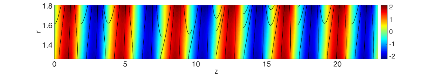
Figure 3: Structure of the axial velocity (top) and the radial magnetic field (bottom) for $Rm=30$, $Ha=100$ and $Re=100$. Both velocity streamlines and magnetic field lines are indicated. Note that the fluid is pumped nearly in synchronism with the traveling magnetic field, similarly to the solution A in Fig. 2.

Figure 4-left shows instantaneous flow profiles as a function of $r$ for two different values of $z$ (note that the same would be obtained for different times at a given $z$ due to the propagative nature of the magnetic field). At $z=1.5$ for instance, the profile is very close to an Hartmann solution, in which the velocity $U_{z}$ (normalized with the wave speed $c$) is nearly equal to $1$ in the whole cross-section. In other words, the flow is pumped in synchronism with the travelling magnetic field. Close to the boundaries however, the flow is forced to vanish due to the no-slip boundary condition, which induces the presence of thin magnetic boundary layers at $r_{i}$ and $r_{o}$. It is important to mention that these layers are not Hartmann boundary layers as generally defined, since the magnetic field varies both in space and time. For instance, as we move to larger $z$, the shear close to the inner cylinder can be strongly reduced: the profile computed at a different location $z=0.4$ (red curve) exhibits a boundary layer near $r_{i}$ roughly $6$ times larger than for $z=1.5$. It is also interesting to note that unlike the imposed magnetic field which creates it, this variation of the boundary layer thickness is not sinusoidal in $z$. Fig. 4-right shows $U_{z}$ as a function of $z$ for different distances from the inner cylinder. It illustrates the strong variation of the thickness of these boundary layers, which consist of large regions where the boundary layer is very thin, alternating with short events of thickened layers (where $B_{r}$ changes sign). It is known that Hartmann layers are linearly stable against axisymmetric disturbances but can be destabilized in $3D$ calculations from transient growth of the two-dimensional perturbations Krasnov04. Here, one may expect that the presence of velocity gradient along $z$ due to the variation of the boundary layer thickness makes the flow more prone to boundary layer instability. In particular, the thickness of these layers do not follow the Hartmann scaling $\delta\sim 1/Ha$ and strongly depends on $Rm$ as well. Although it is beyond the scope of this paper, it would be interesting to compare the stability of the magnetic boundary layers described here with classical results on Hartmann layers.

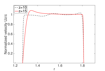
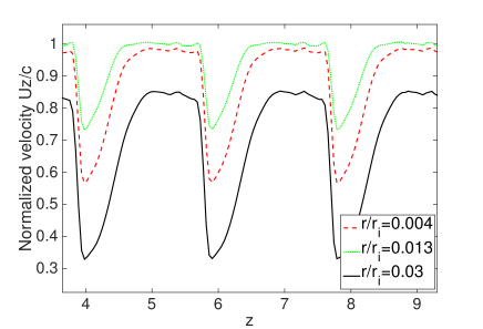
Figure 4: Profiles of the axial velocity field as a function of $r$ (left) and as a function of $z$ for $Rm=30$, $Ha=100$ and $Re=100$. Note the difference with the classical Hartmann boundary layers.

In fact, the fluid velocity strongly depends on the value of the magnetic Reynolds number $Rm$ and the Hartmann number $Ha$. We have performed numerical simulations with different values of $Rm$ and $Ha$, at a fixed value of the kinetic Reynolds number $Re=100$, in order to stay in the laminar regime. At this $Re$, the flow always stays axisymmetric. For each simulation we computed the normalized flow rate through the annular cross-section $S$ of the channel $Q=\frac{1}{S}\int_{S}U_{z}dS$. Figure 5 shows the evolution of the time averaged flow rate as a function of $Rm$, for different values of $Ha$. For the smallest value of the Hartmann number ($Ha=100$, black circle curve), increasing $Rm$ yields a continuous decrease of the fluid velocity, from nearly synchronism ($Q=0.95$) to very small values ($Q\sim 0.02$ at $Rm=200$). Indeed, as $Rm$ is increased at fixed $Re$, the ratio between the Lorentz force and the viscous dissipation decreases, leading to a weaker driving of the flow. The same occurs at low $Rm$ when $Ha$ is decreased. Note that these smooth transitions show no hysteresis, since only one solution seems to be involved.

For larger values of the Hartmann number (for instance $Ha=500$, blue curve), the situation clearly differs: as $Rm$ is increased from $20$ to $350$, the flow is first only weakly modified, from $Q=0.95$ to $Q=0.86$, the velocity of the fluid keeping values relatively close to the wave speed. In this regime, the fluid velocity and the magnetic field have the structure shown in Fig. 3, i.e. of Hartmann-type. However, around $Rm\sim 300$, the flow undergoes a sharp transition from nearly synchronism with the wave to much smaller velocities ($Q=0.25$). During this transition, the total Lorentz force on the fluid also strongly decreases, and the large difference of velocity between the fluid and the wave produces a strong ohmic dissipation. This transition is therefore similar to the saddle-node bifurcation predicted in the model presented in section 2.

This curve can be compared to the calculation from Galaitis76 , which predicts that unstable flows in such pumps may arise when the magnetic Reynolds number based on the slip $Rm_{s}=Rm(1-q)$ becomes sufficiently large. In the inset of Fig.5, we have plotted the bifurcation diagram as a function of $Rm_{s}$. Although this slip Reynolds number seems to slightly rescale our curves, it is clear that it cannot be used as the only rescaling parameter, since the stalling of the pump still depends on the value of the Hartmann number. Note also that the critical values of $Rm$ and $Rm_{s}$ are relatively large in this laminar regime, compared to the prediction $Rm_{s}>1$. We will see in the second part of the paper that these critical numbers strongly decrease with the fluid Reynolds number $Re$, bringing the instability pocket in the accessible parameter range of experimental pumps.

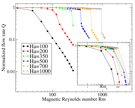
Figure 5: Bifurcation of the axial flow rate as a function of $Rm$, for different values of $Ha$. Note the sharp transition observed at large $Ha,Rm$. Inset: same, but plotted as a function of the slip magnetic Reynolds number (see text))

This transition is shown in more details in Fig. 6, which focuses on the transition observed at $Ha=500$. Black circles correspond to simulations restarted from the calculation performed at a smaller $Rm$, whereas red squares are obtained by continuing simulations performed at larger $Rm$. Depending on initial conditions, the large speed and low speed solutions are bistable on a relatively large range of the magnetic Reynolds number $Rm$ (between $Rm=300$ and $Rm=390$ at $Ha=500$). The transition from synchronous to stalled flows is therefore strongly subcritical, with a strong hysteresis. Note that the bistability involves two solutions with very different spatial structures. In particular, the synchronous solution is associated to strong shear close to the boundaries, but these Hartmann-like boundary layers almost disappear in the stalled regime (see Fig. 6-right), which is closer to a Poiseuille flow.

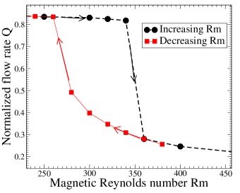
Figure 6: Left: Bifurcation diagram of the axial flow rate as a function of $Rm$, for $Ha=500$. Bistability between two solutions is observed, related to strong hysteresis. Right: radial profiles of the two solutions for $Rm=350$.

Figure 7 summarizes the stability of the flow by showing a colorplot of $Q$ in the parameter space $(Ha-Rm)$. It compares the velocity obtained in our numerical simulations for $Re=100$, interpolated from results of Figure 5, and predictions from the expression given in equation 17 (where only the solution at larger $q$ is computed). All the simulations reported in this figure have been obtained at fixed $Ha$ and increasing $Rm$. It is interesting to note that in both theory and simulations, the marginal stability curve follows $Ha_{c}\propto\sqrt{Rm}$. Because of the bistability described in Fig. 6 and the subcritical nature of the transition, note that a different picture is obtained by decreasing $Rm$ at fixed $Ha$ (and taking the smallest solution of eq. 17). In this case, one observes a critical Hartmann number to follow $Ha_{c}\propto Rm$ instead.

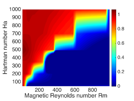
Figure 7: Amplitude of the axial flow rate $Q$ as a function of $Rm$ and $Ha$. Left: theoretical prediction from eq. 17. Right: Global numerical simulations.

Despite the strong assumptions made during the derivation of the analytical model of the previous section, one can see that the behavior of our electromagnetically driven flow in the laminar regime stays very close to theoretical predictions. In particular, note that although strongly irrelevant close to boundaries, this model based on the assumption of an homogeneous velocity in $r$ correctly predicts the shape of the marginal stability curve. This can be understood as a consequence of the Hartmann-type profile observed at the onset of the instability: first, the bulk flow is nearly constant in $r$, in agreement with the theory. Second, since the magnetic boundary layers remain stable (at least for the range of parameters explored here), they do no play a significant role in the transitions, and the dynamics is mainly dominated by the bulk flow only.

However, a closer inspection of the behavior of our simulations shows that not only the magnitude but also the radial structure of the velocity is strongly modified beyond the transition. This modification of the radial profile suggests that the physical mechanism by which the flow becomes unstable may not be captured by the simple theoretical model of section II. In particular, there is no simple explanation for the stability line obtained in Fig. 7. In the next section, we therefore investigate a different type of simulations aiming to clarify the physics of the stalling instability observed in electromagnetic pumps.

V Magnetic flux expulsion

In a real pumps, there is always some pressure loss due to the friction along the pipe, which can in general be related to the averaged velocity of the fluid. In addition to this viscous dissipation, the connection of the pump with the external hydraulic machinery can sometimes induce an additional load acting on the system.

In this section we report another set of simulations, in which both $Rm$ and $Ha$ are kept fixed, but an adverse pressure gradient, modeling an external load, is applied to the pump. Although such a load can have a complex dependence with the velocity, we choose here to use a constant pressure gradient, independent of the flow. These simulations are therefore closer to a real electromagnetic pump, in which the physical properties of the pump are fixed but a variable load is applied on the system. Note that the pressure gradient $P_{ext}$ is now the control parameter for the instability. From an industrial point of view, $Rm$ is still an important control parameter, since its critical value for the stalling instability corresponds to a critical size for large scale induction pump beyond which the flow pumping becomes inefficient.

The results are shown in Figure 8, where the time-averaged normalized flow rate of the fluid is plotted as a function of the amplitude $P_{ext}$ of the load, for $Rm=120$ and $Ha=300$.

Figure 8: Stalling of the flow when submitted to an external load $P_{ext}$, for $Rm=120$ and $Ha=300$. For sufficiently large pressure gradient (in absolute value), the flow can suddenly either accelerate or change direction. Inset: same in log scale.

In this figure, the black dots have been obtained by first performing one simulation at $P_{ext}=0$, and then following this stable branch towards positive and negative $P_{ext}$. In practice, this means that for each value of $P_{ext}$, we used the previous simulation (performed at smaller $|P_{ext}|$) as an initial condition.

Over a large range of $P_{ext}$, the system is relatively independent of the value of the load, and the fluid moves in synchronism with the wave, at a flow speed always larger than $0.8$. For a critical value around $P_{ext}=-0.5$, the flow suddenly bifurcates to a very different regime in which the fluid velocity is pumped backward to the direction of the electromagnetic driving. In addition, this negative velocity strongly depends on the value of the pressure gradient.

Interestingly, an identical transition, but towards large speed flows, occurs if an accelerating pressure gradient is applied to the pump. Note also, that once this bifurcation takes place, the evolution of $Q$ also strongly depends on the pressure gradient.

The next figure helps to understand how this transition is related to the stalling instability described in previous sections. In Fig. 9, the black curve has been obtained by performing simulations in which the flow rate inside the channel is fully determined by some inlet flow rate $Q_{in}$ which is imposed at $z=0$. Since the flow is nearly incompressible, this flow rate is conserved in the whole domain.

By varying $U_{in}$ and reporting the corresponding values of the space and time averaged Lorentz force, we therefore obtain the PQ-characteristic curve of the modeled pump. This curve compares very well to the theoretical prediction shown in section II. As expected, the Lorentz force is nearly zero for $Q=1$, exhibits a very clear maximum before synchronism, and rapidly decreases as the velocity goes away from $Q=1$. Contrary to the theoretical description, the averaged Lorentz force does not vanishes as the velocity goes to strongly negative values. This can be understood as a direct consequence of the no-slip boundary conditions and the associated Hartmann-type boundary layers: close to the boundaries, there is always some region for which $Q$ is close to zero, which corresponds to a strong accelerating Lorentz force.

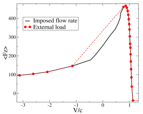
Figure 9: Evolution of the Lorentz force with the flow rate through the annular section. Black line: simulations using an imposed inlet velocity $U_{in}$ (see text). Red dots: simulations performed with an imposed pressure gradient $P_{ext}$, for the same parameters $Rm=120$ and $Ha=300$. The dashed line indicates the jump corresponding to the bifurcation. This PQ characteristic curve is similar to the one predicted from the model in section 2 (see Fig.2).

The red dots of Fig. 9 correspond to simulations shown in Fig. 8, i.e. with an applied pressure gradient $P_{ext}$ rather than an imposed velocity. When $P_{ext}=0$, the only forces applied to the systems are the Lorentz force and a weak dissipation: the pump therefore operates just below synchronism with the wave, the difference being due to the presence of viscous dissipation. As $P_{ext}$ is decreased from $0$ to $-0.5$, this additional external load brakes the flow and pushes the system to lower values of $Q$, which moves on the descending part of the black curve. Note that all the points located on this descending branch $(\partial F_{B}/\partial q<0)$ correspond to stable points, and the large (negative) slope of this branch explains why strong variations of the external load only weakly modify the value of the flow rate. Note however that the electromagnetic force is strongly enhanced during this phase.

For $P_{ext}=-0.5$ however, when the system reaches to maximum value of $F_{B}$, this ’synchronous solution’ looses its stability and the system bifurcates to another stable fixed point corresponding to strongly negative values of the velocity, where the pressure gradient and the viscous dissipation balance the Lorentz force.This new state corresponds to a Poiseuille-type flow mainly imposed by the negative pressure gradient, and only weakly affected by the Lorentz force (compared to Fig. 3). The waviness of the fluid (and therefore the effect of the imposed magnetic field) is still present but its amplitude is negligible compared to the mean value.

From a physical point of view, this transition can be regarded as an instability triggered by magnetic flux expulsion. When operating on the descending part of its characteristic shown in Fig. 9, the pump lies on a stable fixed point, in which the strong Lorentz force balance the force due to the adverse pressure gradient: the mean flow is of Hartmann type. Since a decrease of the flow speed is associated to an increase of the accelerating Lorentz force, this branch is always stabilized by the magnetic tension.

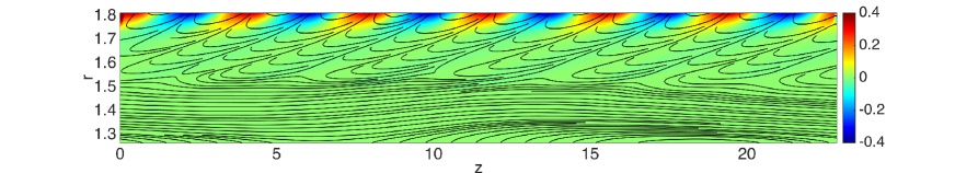
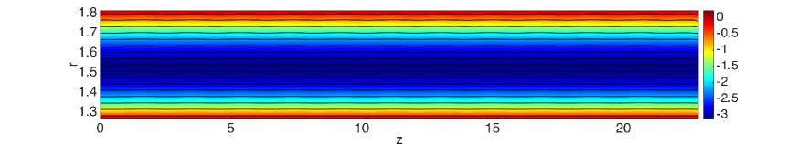
Figure 10: Structure of the axial velocity (top) and the radial magnetic field (bottom) for $Rm=120$, $Ha=100$ and $Re=100$, after the transition ($P_{ext}=-0.6$). Both velocity streamlines and magnetic field lines are indicated.

When the maximum of $F_{B}$ is reached, the system falls on the ascending part of the curve and becomes unstable: on this branch, any perturbation in which the bulk flow slows down implies an increase of the difference of speed between the travelling field and the fluid, and therefore leads to a stronger shear of the magnetic field lines. As a consequence, the magnetic field is expelled away from the bulk flow and the total accelerating Lorentz force decreases, which in turns enhanced the initial braking of the fluid. The magnetic tension cannot counteract the pressure gradient anymore, which amplifies the initial perturbation: the system rapidly moves along the ascending branch of its characteristic until another source of dissipation comes into play. This is the saddle-node bifurcation predicted by the model described in section 2. In our simulations, the instability stops when the viscosity of the fluid counteracts the effect of the adverse pressure gradient, thus leading to the Poiseuille-type regime (corresponding to the solution $A$ in Fig. 2).

Figure 10 shows colorplots of both the radial magnetic field (top) and the axial velocity (bottom) after the saturation of this instability. The top figure clearly illustrates the magnetic field expulsion. First, compared to Fig. 3, the magnetic field lines are clearly tilted by the axial velocity and reconnect into a region very close to the outer cylinder, where the electrical currents are imposed. Second, the colorplot also shows that most of the magnetic energy is expelled from the bulk of the flow and confined close to the outer boundary. The corresponding skin depth is then controlled by the slip between the velocity of the fluid and the wave speed. In this region, the induced magnetic field is then strongly tilted in the streamwise direction, which explains why previous Hartmann-type boundary layer are not generated anymore at the boundaries. Fig. 10-bottom shows the corresponding Poiseuille flow.

Note that the above scenario also applies to configurations in which no pressure gradient is applied, like the simulations described in the previous section. In these simulations, the adverse pressure gradient simply originates from the pressure loss due to viscous friction, and the instability occurs by increasing $Rm$ at fixed pressure gradient (while it is the opposite in the present section).

It is now interesting to relate this flux expulsion scenario to the predictions that can be made for the occurence of the instability. Since flux expulsion is in fact related to the difference of speed between the fluid and the TMF, it is more convenient to describe the behavior of the flow in the reference frame of the TMF, where the velocity of the fluid is $V=(u-c)$. Stalling of the flow occurs when the magnetic tension can no longer stabilize the system, i.e. when the typical spatial variations of the magnetic field in the bulk flow are strong enough, $\delta B/B_{0}>1$. Two different choices can be made on the typical scale of $\delta B$, depending on the force balance in the Navier-Stokes equation. If the flow is laminar, the magnetic tension $\frac{1}{\mu_{0}}(B.\nabla)B$ can be balanced with the viscous force, such that $\delta B\sim\mu_{0}\rho\nu V/B_{0}l$, leading to the following criterion for the occurence of flux expulsion:

$$M_{b}>\sqrt{Re_{s}}$$ (19)

where $Re_{s}=(u-c)l_{0}/\nu=Re(1-q)$ is the kinetic Reynolds number based on the slip. The dimensionless number $M_{b}=(u-c)\sqrt{\mu_{0}\rho}/B_{0}$ is the ratio between the fluid velocity (in the frame of reference of the travelling magnetic field) and the celerity of Alfven waves. As a consequence, $M_{b}$ can be regarded as a magnetic or Alfvenic Mach number, which is an indication of the tendency of the magnetic field to be expelled by the flow (against the restoring magnetic tension).

Note that when applied to large scale electromagnetic pumps, the criterion 19 appears to be extremely restrictive: for a turbulent flow ($Re\sim 10^{6}$) of liquid sodium flowing at $10$m.s^-1, instability may be expected only if $B_{0}<1$Gauss. However, for turbulent flows, it is more reasonable to balance the magnetic force with inertia, giving $\delta B\sim\mu_{0}\rho V^{2}/B_{0}$. In this case, the condition for instability simply reduces to:

$$M_{b}>1$$ (20)

This new condition, only valid for turbulent flows, is different from the classical prediction $Rm_{s}>1$ of the simple block velocity model presented in the first section of this article, and predicts flux expulsion for much larger magnetic field than the viscous scaling discussed above. It provides an interesting new criterion, very simple, for predicting the occurrence of the stalling instability. An important point is that this criterion is local, independently of the size of the system.

Fig. 11 shows the evolution of the normalized flow rate as a function of $M_{b}$. Compared to Fig. 5, the use of this new dimensionless number provides a very good rescaling of our data, suggesting that the Magnetic Mach number is more prone to predict the occurence of the stalling instability. The collapse of the points naturally disappears after the transition, where a non-magnetized Poiseuille regime is instead achieved. Despite the small values of $Re/Ha$ in our simulations, the transition seems to follows prediction of eq. (20) rather than eq. (19). This suggests that the laminar/turbulent transition occurs for a kinetic Reynolds number much smaller than the one generally observed in Hartmann flows, and follows a different scaling.

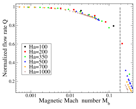
Figure 11: Bifurcation of the axial flow rate as a function of the magnetic Mach number $M_{b}$, for different values of $Ha$. Note the rescaling of the points and the sharp transition observed at a given value of $M_{b}$.

Finally, note that the above discussion using the Magnetic Mach number concerns the transition from synchronous to stalled flows, but implicitly suppose a large magnetic Reynolds number. Indeed, the hysteresis related to the saddle-node bifurcation is only observed for large magnetic Reynolds number: in order to observe a discontinuous jump of the flow rate at $M_{b}\sim 1$, it is therefore necessary to have also $Rm_{s}>1$ at the transition.

VI Discussion and conclusion

We reported a numerical study of the MHD flow driven by a travelling magnetic field (TMF) in an annular channel. This configuration aims to reproduce the flow of liquid metals generated inside annular linear induction electromagnetic pumps. The purpose of this first part was to compare laminar simulations to some simple theoretical predictions, and to clarify the physical mechanisms by which such flows could become unstable at large magnetic Reynolds numbers. We have shown that at sufficiently large $Rm$ and $Ha$, the flow undergoes a transition similar to the stalling of an asynchronous motor. For the small values of the kinetic Reynolds number used here, we have shown that several aspects of the theoretical description based on an homogeneous velocity remains valid: this model is able to correctly predict the shape of the PQ characteristic, and the amplitude of both velocity and magnetic field.

We have also identified magnetic flux expulsion as the physical mechanism by which the instability occurs. This is particularly clear when an external pressure gradient is applied to the system, and a sharp transition from Hartmann-like synchronous flows to Poiseuille-type counter-flows is observed.

It is interesting to note that the behavior observed in these simulations presents strong analogies with two analytical models proposed by Gimblett79 and by Moffatt82 . In the first one, the rotation of an electrically conducting solid disk in a transverse magnetic field is investigated. The existence of a forbidden band of rotation rates for a given driving torque is predicted. In the second article, the authors study a pressure-driven flow along a rectangular channel in the presence of a (steady) applied magnetic field which is periodic in the streamwise direction. They find that for a critical pressure gradient, a runaway situation is observed in which the flow rapidly increases to larger values. This prediction has been recently confirmed by direct numerical simulations performed in a plane channel flow Bandaru15 . Our calculations and the interpretation given in the previous section suggest that the exact same mechanism occurs in the case of a linear induction electromagnetic pump: as the difference of speed between the fluid and the wave increases, magnetic field is expelled outside the conductor and leads to a stalled regime dominated by viscosity.

Moreover, when the aforementioned studies are transposed to our problem, these calculations imply that if an accelerating pressure gradient is applied to an induction pump, a transition opposite to the stalling instability should be observed for sufficiently large pressure gradient: the flow bifurcates from an Hartmann-type regime close to synchronism, toward a much faster Poiseuille flow ultimately controlled by viscous dissipation. This scenario has indeed been observed in our simulations (the transition reported in Fig. 8 for $P_{ext}>1.25$).

In both cases (stalling or acceleration), magnetic flux expulsion associated with reconnection of field lines is responsible for the occurrence of the instability. This interpretation allows us to suggest that the Magnetic Mach number $M_{b}$ defined in the last section is controlling the generation of these instabilities.

Finally, it is crucial to note that industrial pumps and experimental facilities are much more complex than the simple simulations reported here. Among the most important differences, one is related to the presence of inlet/outlet boundary conditions, and the other to the very large fluid Reynolds numbers involved, which implies highly turbulent flows. In a second article Rodriguez16 , we will therefore report numerical simulations done at larger Reynolds numbers and with more realistic axial boundary conditions. We will show how the bifurcation described here leads to inhomogeneous flows at larger fluid Reynolds number.

- (1)
- (2) Z. Stelzer,D. Cebron, S. Miralles, S. Vantieghem, J. Noir, P. Scarfe, A. Jackson, Experimental and numerical study of electrically driven magnetohydrodynamic flow in a modified cylindrical annulus. I. Base flow, Phys. fluids 27, 077101 (2015)
- (3) A.M. Andreev et al., Results of an experimental investigation of electromagnetic pumps for the BOR-60 facility, Magnitnaya Gidrodinamika ,1, 61-67 (English translation) (1988)
- (4) G.B. Kliman, Large electromagnetic pump, Electr. Mach. Electromech., 3, 129- 142 (1979)
- (5) H. Ota et al., Development of 160 m3/min large capacity sodium-immersed self-cooled electromagnetic pump , J. Nucl. Sci. Tech., 41,511-523 (2004)
- (6) Gailitis A. and O. Lielausis, Instability of homogeneous velocity distribution in an induction-type mhd machine, Magnetohydrodynamics, 1, 69-79 (1976). Translation from Magnitnaya Gidrodinamika 1, 87-101 (1975).
- (7) Kirillov, I.R., Ogorodnikov, A.P., Ostapenko, V.P. ,Local characteristics of a cylindrical induction pump for Rms larger than 1 , English translation from Magnitnaya Gidrodinamika 2, 107- 113 (1980)
- (8) Araseki H., Kirillov I., Preslitsky G. and Ogorodnikov A. P., Double-supply-frequency pressure pulsation in annular linear induction pump. Part I. Measurement and numerical analysis., Nucl. Engin. and Design 195, 85-100 (2000)
- (9) Araseki, H., Kirillov, I.R., Preslitsky, G.V., Ogorodnikov, Magnetohydrodynamic instability in annular linear induction pump:: Part I. Experiment and numerical analysis, A.P., Nucl. Eng. Des. 227, 29- 50. (2004)
- (10) Gonzales et al, HERACLES: a three-dimensional radiation hydrodynamics code, Astronomy and Astrophysics, 464, 429-435 (2006).
- (11) W. Liu, J. Goodman, and H. Ji, Simulations of magnetorotational instability in a magnetized Couette flow, Astrophys. J. 643, 306 (2006).
- (12) W. Liu, Numerical study of the magnetorotational instability in Princeton MRI experiment, Astrophys. J. 684, 515 (2008).
- (13) C. Gissinger, H. Ji and J. Goodman, The role of boundaries in the Magnetorotational instability, Phys. Fluids. 24, 074109 (2012).
- (14) C.G. Gimblett and R.S. Peckover, On the Mutual Interaction between Rotation and Magnetic Fields for Axisymmetric Bodies, Proc. Roy. Soc. A, 368, 75-97 (1979)
- (15) H.Kamkar and H.K.Moffatt, J. Fluid Mech., A dynamic runaway effect associated with flux expulsion in magnetohydrodynamic channel flow, 121,107-122 (1982)
- (16) V. Bandaru, J. Pracht, T. Boeck, J. Schumacher, Simulation of flux expulsion and associated dynamics in a two-dimensional magnetohydrodynamic channel flow, ArXiv (2015)
- (17) P. Rodriguez-Imazio, C. Gissinger, S. Fauve, Physics of Fluids (2016)