Abstract

The nested off-diagonal Bethe ansatz is generalized to study the quantum spin chain associated with the $SU_{q}(3)$ $R$-matrix and generic integrable non-diagonal boundary conditions. By using the fusion technique, certain closed operator identities among the fused transfer matrices at the inhomogeneous points are derived. The corresponding asymptotic behaviors of the transfer matrices and their values at some special points are given in detail. Based on the functional analysis, a nested inhomogeneous $T-Q$ relations and Bethe ansatz equations of the system are obtained. These results can be naturally generalized to cases related to the $SU_{q}(n)$ algebra.

PACS: 75.10.Pq, 02.30.Ik, 71.10.Pm

Keywords: Spin chain; reflection equation; Bethe ansatz; $T-Q$ relation

1 Introduction

Exact solution is a very important issue in studies of statistical mechanics, condensed matter physics, quantum field theory and mathematical physics [1, 2] since those results can provide important benchmarks for understanding physical effects in a variety of systems. The coordinate Bethe ansatz and the algebraic Bethe ansatz are two powerful methods to obtain the exact solution of the integrable systems [3, 4, 5, 6, 7]. With these methods, many interesting exactly solvable models, such as the one-dimensional Hubbard model, supersymmetric $t-J$ model, Heisenberg spin chain and the $\delta$-potential quantum gas model, were exactly solved. For integrable systems with $U(1)$ symmetry, it is easy to find a reference state and these conventional Bethe ansatz can be applied to. Indeed, most of the previous studies focus on periodic or diagonal open boundary conditions without breaking the $U(1)$ symmetry. However, there exists another kind of integrable systems which does not have the $U(1)$ symmetry, such as the integrable systems with generic off-diagonal boundary reflections. Because the reference state of this kind of integrable system is absent, the conventional Bethe ansatz methods are failed. On the other hand, many interesting phenomena arise in this kind of systems, such as the topological elementary excitations in the spin-1/2 torus [8], spiral phase in the Heisenberg model with unparallel boundary magnetic field [9] and stochastic process in non-equilibrium statistical mechanics [10, 11, 12]. Motivated by these important applications, many interesting methods such as the q-Onsager algebra [13, 14, 15], the modified algebraic Bethe ansatz [16, 17, 18, 19] and the Sklyanin’s separation of variables (SoV) [20, 21, 22, 23, 24] were also applied to some integrable models without $U(1)$ symmetry. Other interesting progress can be found in [25, 26, 27, 28, 29].

Recently, a new approach, i.e., the off-diagonal Bethe ansatz (ODBA) [8] was proposed to obtain exact solutions of generic integrable models either with or without $U(1)$ symmetry. Several long-standing problems were then solved [30, 31, 32, 33, 34, 35, 36] via this method. For comprehensive introduction to this method we refer the readers to [37]. In order to study the high rank integrable models, the nested version of ODBA has been proposed for the isotropic (or rational) models [33]. In this paper, we study the anisotropic rank-2 spin model with generic integrable boundary conditions. Here the $R$-matrix is the trigonometric one associated with the $SU_{q}(3)$ algebra and the boundary reflection matrices are the most generic reflection matrices which have non-vanishing off-diagonal elements. Because the off-diagonal elements of the reflection matrices break the $U(1)$ symmetry, the exact solution of the system has been missing even its integrability was known for many years ago. By using the fusion technique and nested ODBA, we successfully obtain the closed operator identities, the values at the special points and the asymptotic behaviors. Based on them, we construct the nested inhomogeneous $T-Q$ relation and obtain the eigenvalue of the transfer matrix thus the energy spectrum of the system. These results can be generalized to multiple components spin chains related to more higher rank algebra cases.

The paper is organized as follows. Section 2 is the general description of the model. The $SU_{q}(3)$ $R$-matrix and corresponding generic integral non-diagonal boundary reflection matrices are introduced. In Section 3, by using the fusion technique, we derive the closed operator identities for the fused transfer matrices and the quantum determinant. The asymptotic behaviors of the fused transfer matrix and their values at special points are also obtained. In section 4, we list some necessary functional relations which are used to determine the eigenvalues. Section 5 is devoted to the construction of the nested inhomogeneous $T-Q$ relation and the Bethe ansatz equations. In section 6, we summarize our results and give some discussions. Some results related to the other types of the general off-diagonal boundary reflections are given in Appendix.

2 The model

Throughout, ${\rm\bf V}$ denotes a three-dimensional linear space and let $\{|i\rangle,i=1,2,3\}$ be an orthonormal basis of it. We shall adopt the standard notations. For any matrix $A\in{\rm End}({\rm\bf V})$, $A_{j}$ is an embedding operator in the tensor space ${\rm\bf V}\otimes{\rm\bf V}\otimes\cdots$, which acts as $A$ on the $j$-th space and as identity on the other factor spaces. For $B\in{\rm End}({\rm\bf V}\otimes{\rm\bf V})$, $B_{ij}$ is an embedding operator of $B$ in the tensor space, which acts as identity on the factor spaces except for the $i$-th and $j$-th ones.

The $R$-matrix $R(u)\in{\rm End}({\rm\bf V}\otimes{\rm\bf V})$ used in this paper is the trigonometric one associated with the $SU_{q}(3)$ algebra, which was first proposed by Perk and Shultz [38] and further studied in [39, 40, 41, 42, 43],

$$R_{12}(u)=\left(\begin{array}[]{r|r|r}{\begin{array}[]{rrr}a(u)&&\\ &b(u)&\\ &&b(u)\end{array}}&{\begin{array}[]{lll}&&\\ c(u)&}{&}{\\ }{&}{&}{\end{array}}&{\begin{array}[]{lll}&&\\ &&\\ c(u)&}{&}{\end{array}}\\[12.0pt] \hline\cr{\begin{array}[]{rrr}&d(u)&\\ &&}{\hfil\\ &&\end{array}}&{\begin{array}[]{ccc}b(u)&&\\ &a(u)&\\ &&b(u)\end{array}}&{\begin{array}[]{lll}&&\\ }{&}{&}{\\ &c(u)&}{\end{array}}\\[12.0pt] \hline\cr{\begin{array}[]{ccc}&&d(u)\\ &&\\ &&\end{array}}&{\begin{array}[]{ccc}&&\\ &&d(u)\\ &&\end{array}}&{\begin{array}[]{ccc}b(u)&&\\ &b(u)&\\ &&a(u)\end{array}}\end{array}\right),$$ (2.31)

where the matrix elements are

$$a(u)=\sinh(u+\eta),\quad b(u)=\sinh(u),$$ (2.32)

$$c(u)=e^{u}\sinh\eta,\quad d(u)=e^{-{u}}\sinh\eta.$$ (2.33)

The $R$-matrix satisfies the quantum Yang-Baxter equation (QYBE)

$$R_{12}(u_{1}-u_{2})R_{13}(u_{1}-u_{3})R_{23}(u_{2}-u_{3})=R_{23}(u_{2}-u_{3})R_{13}(u_{1}-u_{3})R_{12}(u_{1}-u_{2}),$$ (2.34)

and possesses the following properties,

$$\mbox{ Initial condition}:\,R_{12}(0)=\sinh\eta P_{12},$$ (2.35)

$$\mbox{ Unitarity relation}:\,R_{12}(u)R_{21}(-u)=\rho_{1}(u)\,\times{\rm id},$$ (2.36)

$$\mbox{ Crossing Unitarity relation}:\,R_{12}^{t_{1}}(u)\,{\cal M}_{1}\,R_{21}^{t_{1}}(-u-3\eta)\,{\cal M}_{1}^{-1}=\rho_{2}(u)\,\times{\rm id},$$ (2.37)

$$\mbox{ PT-symmetry}:\,R_{21}(u)=R^{t_{1}\,t_{2}}_{12}(u),$$ (2.38)

$$\mbox{ Periodicity}:\,R_{12}(u+i\pi)=-R_{12}(u).$$ (2.39)

Here $R_{21}(u)=P_{12}R_{12}(u)P_{12}$ with $P_{12}$ being the usual permutation operator and $t_{i}$ denotes transposition in the $i$-th space. The functions $\rho_{1}(u)$, $\rho_{2}(u)$ and the crossing matrix ${\cal M}$ are given by

$$\rho_{1}(u) = -\sinh({u}-\eta)\sinh({u}+\eta),$$ (2.40)

$$\rho_{2}(u) = -\sinh({u})\sinh({u}+3\eta),$$ (2.41)

$${\cal M} = \left(\begin{array}[]{ccc}e^{4\eta}&&\\ &e^{2\eta}&\\ &&1\end{array}\right).$$ (2.45)

It is easy to check that the $R$-matrix (2.31) also has the following properties

$${\cal M}_{1}\,{\cal M}_{2}\,R_{12}(u)\,{\cal M}_{1}^{-1}\,{\cal M}_{2}^{-1}=R_{12}(u).$$ (2.46)

Let us introduce the reflection matrix $K^{-}(u)$ and its dual one $K^{+}(u)$. The former satisfies the reflection equation (RE)

$$R_{12}(u_{1}-u_{2})K^{-}_{1}(u_{1})R_{21}(u_{1}+u_{2})K^{-}_{2}(u_{2})$$

$$~{}~{}~{}~{}~{}~{}=K^{-}_{2}(u_{2})R_{12}(u_{1}+u_{2})K^{-}_{1}(u_{1})R_{21}(u_{1}-u_{2}),$$ (2.47)

and the latter satisfies the dual RE

$$R_{12}(u_{2}-u_{1})K^{+}_{1}(u_{1}){\cal M}_{1}^{-1}R_{21}(-u_{1}-u_{2}-3\eta){\cal M}_{1}K^{+}_{2}(u_{2})$$

$$~{}~{}~{}~{}~{}~{}=K^{+}_{2}(u_{2}){\cal M}_{2}^{-1}R_{12}(-u_{1}-u_{2}-3\eta){\cal M}_{2}K^{+}_{1}(u_{1})R_{21}(u_{2}-u_{1}).$$ (2.48)

In this paper we consider the generic non-diagonal $K$-matrices $K^{-}(u)$ found in [44, 45, 46]. There are three kinds of reflecting $K$-matrix:

$$({\rm{I}}):K^{-}(u)=\left(\begin{array}[]{ccc}e^{u}\sinh(\zeta-u)+ce^{2u}\sinh(2u)&0&0\\[6.0pt] 0&e^{u}\sinh(\zeta-u)&c_{1}\sinh(2u)\\[6.0pt] 0&c_{2}\sinh(2u)&e^{-u}\sinh(\zeta+u)\end{array}\right),$$ (2.52)

with the constraint

$$c^{2}=c_{1}c_{2}+ce^{\zeta}.$$

Thus the four boundary parameters $c$, $c_{1}$ $c_{2}$ and $\zeta$ are not independent with each other.

$$({\rm{II}}):K^{-}(u)=\left(\begin{array}[]{ccc}e^{u}\sinh(\zeta-u)&0&c_{1}\sinh(2u)\\[6.0pt] 0&e^{u}\sinh(\zeta-u)+c\sinh(2u)&0\\[6.0pt] c_{2}\sinh(2u)&0&e^{-u}\sinh(\zeta+u)\end{array}\right),$$ (2.56)

with the constraint

$$c^{2}=c_{1}c_{2}+ce^{-\zeta}.$$

$${({\rm{III}}):K^{-}(u)=\left(\begin{array}[]{ccc}e^{u}\sinh(\zeta-u)&c_{1}\sinh(2u)&0\\[6.0pt] c_{2}\sinh(2u)&e^{-u}\sinh(\zeta+u)&0\\[6.0pt] 0&0&e^{-u}\sinh(\zeta+u)+ce^{-2u}\sinh(2u)\end{array}\right),}$$ (2.60)

with the constraint

$$c^{2}=c_{1}c_{2}-ce^{\zeta}.$$

The dual non-diagonal reflection matrix $K^{+}(u)$ is given by

$$K^{+}(u)={\cal M}K^{-}(-u-3\eta/2)\left|{}_{(\zeta,c,c_{1},c_{2})\rightarrow(\zeta^{\prime},c^{\prime},c_{1}^{\prime},c_{2}^{\prime})}\right..$$ (2.61)

In order to construct the model’s Hamiltonian of the system, we first introduce the “row-to-row” (or one-row) monodromy matrices $T_{0}(u)$ and $\hat{T}_{0}(u)$

$$T_{0}(u) = R_{0N}(u-\theta_{N})R_{0\,N-1}(u-\theta_{N-1})\cdots R_{01}(u-\theta_{1}),$$ (2.62)

$$\hat{T}_{0}(u) = R_{10}(u+\theta_{1})R_{20}(u+\theta_{2})\cdots R_{N0}(u+\theta_{N}),$$ (2.63)

where $\{\theta_{j},j=1,\cdots,N\}$ are the inhomogeneous parameters and $N$ is the number of sites. The one-row monodromy matrices are the $3\times 3$ matrices in the auxillary space $0$ and their elements act on the quantum space ${\rm\bf V}^{\otimes N}$. For the system with open boundaries, we need to define the double-row monodromy matrix $\mathbb{T}_{0}(u)$

$$\mathbb{T}_{0}(u)=T_{0}(u)K^{-}_{0}(u)\hat{T}_{0}(u).$$ (2.64)

Then the transfer matrix of the system is constructed as [7]

$$t(u)=tr_{0}\{K^{+}_{0}(u)\mathbb{T}_{0}(u)\}.$$ (2.65)

From the QYBE (2.34), RE (2.47) and dual RE (2.48), one can prove that the transfer matrices with different spectral parameters commute with each other, $[t(u),t(v)]=0$. Therefore, $t(u)$ serves as the generating functional of all the conserved quantities of the system. The model Hamiltonian can be constructed by taking the derivative of the logarithm of the transfer matrix of the system

$$H=\sinh\eta\frac{\partial\ln t(u)}{\partial u}|_{u=0,\{\theta_{j}\}=0}.$$ (2.66)

3 Fusion

Following [33], we apply the fusion technique [47, 48, 49] to study the present model. The fusion procedure will lead to the desired operator identities to determine the spectrum of the transfer matrix $t(u)$ given by (2.65). For this purpose, let us introduce the following vectors in the tensor space ${\rm\bf V}\otimes{\rm\bf V}$ similarly as [36]

$$|\Phi^{(1)}_{12}\rangle = \frac{1}{\sqrt{2e^{\eta}\cosh\eta}}(|1,2\rangle-e^{\eta}|2,1\rangle),$$

$$|\Phi^{(2)}_{12}\rangle = \frac{1}{\sqrt{2e^{\eta}\cosh\eta}}(|1,3\rangle-e^{\eta}|3,1\rangle),$$ (3.1)

$$|\Phi^{(3)}_{12}\rangle = \frac{1}{\sqrt{2e^{\eta}\cosh\eta}}(|2,3\rangle-e^{\eta}|3,2\rangle),$$

in the tensor space ${\rm\bf V}\otimes{\rm\bf V}$ and

$$|\Phi_{123}\rangle = \frac{1}{\sqrt{2e^{3\eta}(2\cosh\eta+\cosh 3\eta)}}(|1,2,3\rangle-e^{\eta}|1,3,2\rangle+e^{2\eta}|3,1,2\rangle$$ (3.2)

$$-e^{\eta}|2,1,3\rangle+e^{2\eta}|2,3,1\rangle-e^{3\eta}|3,2,1\rangle),$$

in the tensor space ${\rm\bf V}\otimes{\rm\bf V}\otimes{\rm\bf V}$. The associated projectors are

$$P_{12}^{-}=|\Phi^{(1)}_{12}\rangle\langle\Phi^{(1)}_{12}|+|\Phi^{(2)}_{12}\rangle\langle\Phi^{(2)}_{12}|+|\Phi^{(3)}_{12}\rangle\langle\Phi^{(3)}_{12}|,$$ (3.3)

$$P_{123}^{-}=|\Phi_{123}\rangle\langle\Phi_{123}|.$$ (3.4)

Direct calculation shows that the $R$-matrix given by (2.31) at some degenerate points are proportional to the projectors,

$$R_{12}(-\eta)=P^{-}_{12}\times S_{12},\quad R_{12}(-\eta)R_{13}(-2\eta)R_{23}(-\eta)=P_{123}^{-}\times S_{123},$$ (3.5)

where the diagonal matrices $S_{12}$ and $S_{123}$ are given by

$$S_{12}=-\sinh 2\eta\times Diag[1,e^{\eta},e^{\eta},e^{-\eta},1,e^{\eta},e^{-\eta},e^{-\eta},1],$$ (3.6)

$$S_{123}=-2\sinh 2\eta\sinh^{2}\eta(2\cosh\eta+\cosh 3\eta)\times Diag[1,1,1,1,1,e^{3\eta},1,e^{\eta},1,1,1,e^{\eta},$$

$$\hskip 28.45274pt1,1,1,e^{-\eta},1,1,1,e^{-\eta},1,e^{-3\eta},1,1,1,1,1].$$ (3.7)

The fused transfer matrices are defined as

$$t_{m}(u)=tr_{12\cdots m}\{K^{+}_{<12\cdots m>}(u)T_{<12\cdots m>}(u)K^{-}_{<12\cdots m>}(u)\hat{T}_{<12\cdots m>}(u)\},\quad m=1,2,3,$$ (3.8)

where

$$K^{+}_{12\cdots m}(u)=K^{+}_{<2\cdots m>}(u-\eta){\cal M}_{2}^{-1}R_{1m}(-2u+(m-1)\eta-3\eta)$$

$$\qquad\qquad\times R_{1m-1}(-2u+(m-2)\eta-3\eta)\cdots R_{12}(-2u+\eta-3\eta){\cal M}_{2}K^{+}_{1}(u),$$ (3.9)

$$K^{+}_{<12\cdots m>}(u)=P^{-}_{12\cdots m}K^{+}_{12\cdots m}(u)P^{-}_{mm-1\cdots 1},$$ (3.10)

$$K^{-}_{12\cdots m}(u)=K^{-}_{1}(u)R_{21}(2u-\eta)$$

$$\qquad\qquad\qquad\times R_{31}(2u-2\eta)\cdots R_{m1}(2u-(m-1)\eta)K^{-}_{<2\cdots m>}(u-\eta),$$ (3.11)

$$K^{-}_{<12\cdots m>}(u)=P^{-}_{mm-1\cdots 1}K^{-}_{12\cdots m}(u)P^{-}_{12\cdots m},$$ (3.12)

$$T_{<12\cdots m>}(u)=P^{-}_{mm-1\cdots 1}T_{1}(u)T_{2}(u-\eta)\cdots T_{m}(u-(m-1)\eta)P^{-}_{mm-1\cdots 1},$$ (3.13)

$$\hat{T}_{<12\cdots m>}(u)=P^{-}_{12\cdots m}\hat{T}_{1}(u)\hat{T}_{2}(u-\eta)\cdots\hat{T}_{m}(u-(m-1)\eta)P^{-}_{12\cdots m},$$ (3.14)

and the notation $t_{1}(u)=t(u)$ is used. By repeatedly using the QYBE (2.34), the RE (2.47), the dual RE (2.48) and the definition (3.8), one can prove that all these fused transfer matrices are commutative with each other

$$[t_{m}(u),t_{k}(v)]=0,\quad m,k=1,2,3.$$ (3.15)

Thus they have the common eigenstates. Furthermore, we find that the transfer matrix given by (3.8) satisfies the following operator production identities

$$t(\pm\theta_{j})t_{m}(\pm\theta_{j}-\eta)={t_{m+1}(\pm\theta_{j})}{\prod_{k=1}^{m}\rho^{-1}_{2}(\pm 2\theta_{j}-k\eta)},\,\,j=1,\ldots,N,\,\,m=1,2,$$ (3.16)

$$t_{2}(\pm\theta_{j}+\eta)=0,\quad j=1,\cdots,N.$$ (3.17)

We note that the fused transfer matrix $t_{3}(u)$ equals to its quantum determinant multiplying the unity matrix. Thus the operators production identities (3.16) are closed. The explicit form of the fused transfer matrix $t_{3}(u)$ reads

$$t_{3}(u)=\Delta_{q}(u)\times{\rm id}=\Delta_{q}\{T(u)\}\Delta_{q}\{\hat{T}(u)\}\Delta_{q}\{K^{+}(u)\}\Delta_{q}\{K^{-}(u)\}\times{\rm id},$$ (3.18)

where $\Delta_{q}\{T(u)\}$, $\Delta_{q}\{\hat{T}(u)\}$, $\Delta_{q}\{K^{+}(u)\}$ and $\Delta_{q}\{K^{-}(u)\}$ are the quantum determinants of the matrices $T(u)$, $\hat{T}(u)$, $K^{+}(u)$ and $K^{-}(u)$, respectively. The quantum determinants of the one-row monodromy matrices are

$$\Delta_{q}\{T(u)\}=\prod_{l=1}^{N}\sinh(u-\theta_{l}+\eta)\sinh(u-\theta_{l}-\eta)\sinh(u-\theta_{l}-2\eta),$$ (3.19)

$$\Delta_{q}\{\hat{T}(u)\}=\prod_{l=1}^{N}\sinh(u+\theta_{l}+\eta)\sinh(u+\theta_{l}-\eta)\sinh(u+\theta_{l}-2\eta).$$ (3.20)

The quantum determinant of the reflecting matrix (I) given by (2.52) is

$$\Delta_{q}\{K^{-}(u)\} = -(e^{u-\eta}\sinh(\zeta-u+\eta)+ce^{2u-2\eta}\sinh(2u-2\eta))$$ (3.21)

$$\times(\sinh(\zeta-u)\sinh(\zeta+u)-c_{1}c_{2}\sinh(2u)\sinh(2u))$$

$$\times\sinh(2u-2\eta)\sinh(2u-3\eta)\sinh(2u-4\eta)$$

$$= -(e^{u-\eta}\sinh(\zeta-u+\eta)+ce^{2u-2\eta}\sinh(2u-2\eta))$$

$$\times(e^{u}\sinh(\zeta-u)+ce^{2u}\sinh(2u))$$

$$\times(e^{-u}\sinh(\zeta+u)-ce^{-2u}\sinh(2u))$$

$$\times\sinh(2u-2\eta)\sinh(2u-3\eta)\sinh(2u-4\eta).$$

The quantum determinant of the reflecting matrix (II) given by (2.56) is

$$\Delta_{q}\{K^{-}(u)\} = -(e^{u-\eta}\sinh(\zeta-u+\eta)+c\sinh(2u-2\eta))$$ (3.22)

$$\times(\sinh(\zeta-u)\sinh(\zeta+u)-c_{1}c_{2}\sinh(2u)\sinh(2u))$$

$$\times\sinh(2u-2\eta)\sinh(2u-3\eta)\sinh(2u-4\eta)$$

$$= -(e^{u-\eta}\sinh(\zeta-u+\eta)+c\sinh(2u-2\eta))$$

$$\times(e^{u}\sinh(\zeta-u)+c\sinh(2u))$$

$$\times(e^{-u}\sinh(\zeta+u)-c\sinh(2u))$$

$$\times\sinh(2u-2\eta)\sinh(2u-3\eta)\sinh(2u-4\eta).$$

The quantum determinant of the reflecting matrix (III) given by (2.60) is

$$\Delta_{q}\{K^{-}(u)\} = -(e^{-u+\eta}\sinh(\zeta+u-\eta)+ce^{-2u+2\eta}\sinh(2u-2\eta))$$ (3.23)

$$\times(\sinh(\zeta-u)\sinh(\zeta+u)-c_{1}c_{2}\sinh(2u)\sinh(2u))$$

$$\times\sinh(2u-2\eta)\sinh(2u-3\eta)\sinh(2u-4\eta)$$

$$= -(e^{-u+\eta}\sinh(\zeta+u-\eta)+ce^{-2u+2\eta}\sinh(2u-2\eta))$$

$$\times(e^{u}\sinh(\zeta-u)-ce^{2u}\sinh(2u))$$

$$\times(e^{-u}\sinh(\zeta+u)+ce^{-2u}\sinh(2u))$$

$$\times\sinh(2u-2\eta)\sinh(2u-3\eta)\sinh(2u-4\eta).$$

The quantum determinant of the dual reflecting matrices $K^{+}(u)$ can be obtained by the mapping

$$\Delta_{q}\{K^{+}(u)\}=e^{6\eta}\Delta_{q}\{K^{-}(-u+\frac{\eta}{2})\}|_{(c,\zeta\rightarrow c^{\prime},\zeta^{\prime})}.$$

Then the equation (3.18) can be proved easily based on the facts

$$T_{<123>}(u)=\Delta_{q}\{T(u)\}P^{-}_{321},$$ (3.24)

$$\hat{T}_{<123>}(u)=\Delta_{q}\{\hat{T}(u)\}P^{-}_{123},$$ (3.25)

$$K^{-}_{<123>}(u)=\Delta_{q}\{K^{-}(u)\}|\Phi_{321}\rangle\langle\Phi_{123}|,$$ (3.26)

$$K^{+}_{<123>}(u)=\Delta_{q}\{K^{+}(u)\}|\Phi_{123}\rangle\langle\Phi_{321}|.$$ (3.27)

Form the definition of fused transfer matrices (3.8), the corresponding asymptotic behaviors can be calculated directly. Obviously, different reflection parameters will give different asymptotic behaviors. Without losing the generality, we consider the case corresponding to the reflection matrices $K^{\pm}(u)$ given by (2.52) and (2.61) and the details for the results for the other cases will be presented in Appendix. Then the asymptotic behaviors read

$$t_{1}(u)|_{u\rightarrow+\infty} = -\frac{1}{4^{N+1}}e^{(2N+4)u+3\eta}\left[c\frac{c_{1}^{\prime}c_{2}^{\prime}}{c^{\prime}}e^{\eta}e^{2\eta{\cal{Q}}^{(1)}}\right.$$ (3.28)

$$+\left.(c_{1}c_{2}^{\prime}+c_{1}^{\prime}c_{2}e^{2\eta})e^{N\eta}e^{-\eta{\cal{Q}}^{(1)}}\right]+\cdots,$$

$$t_{1}(u)|_{u\rightarrow-\infty} = -\frac{1}{4^{N+1}}e^{-(2N+4)u-3\eta}\left[c^{\prime}\frac{c_{1}c_{2}}{c}e^{\eta}e^{-2\eta{\cal{Q}}^{(1)}}\right.$$ (3.29)

$$+\left.(c_{1}c_{2}^{\prime}+c_{1}^{\prime}c_{2}e^{2\eta})e^{-N\eta}e^{\eta{\cal{Q}}^{(1)}}\right]+\cdots,$$

$$t_{2}(u)|_{u\rightarrow+\infty} = -\frac{1}{4^{2N+3}}e^{4(N+3)u+4\eta}c\frac{c_{1}^{\prime}c_{2}^{\prime}}{c^{\prime}}\left[c^{\prime}\frac{c_{1}c_{2}}{c}e^{\eta}e^{-2\eta{\cal{Q}}^{(1)}}\right.$$ (3.30)

$$+\left.(c_{1}c_{2}^{\prime}+c_{1}^{\prime}c_{2}e^{2\eta})e^{-N\eta}e^{\eta{\cal{Q}}^{(1)}}\right]+\cdots,$$

$$t_{2}(u)|_{u\rightarrow-\infty} = -\frac{1}{4^{2N+3}}e^{-4(N+3)u-2\eta}c^{\prime}\frac{c_{1}c_{2}}{c}\left[c\frac{c_{1}^{\prime}c_{2}^{\prime}}{c^{\prime}}e^{\eta}e^{2\eta{\cal{Q}}^{(1)}}\right.$$ (3.31)

$$+\left.(c_{1}c_{2}^{\prime}+c_{1}^{\prime}c_{2}e^{2\eta})e^{N\eta}e^{-\eta{\cal{Q}}^{(1)}}\right]+\cdots,$$

where the operator ${\cal{Q}}^{(1)}$ is

$${\cal{Q}}^{(1)}=\sum_{l=1}^{N}E^{11}_{l},\quad E^{11}=\left(\begin{array}[]{ccc}1&0&0\\ 0&0&0\\ 0&0&0\end{array}\right).$$ (3.35)

In the derivation, the relations $c(c-e^{\zeta})=c_{1}c_{2}$ and $c^{\prime}(c^{\prime}-e^{\zeta^{\prime}})=c_{1}^{\prime}c_{2}^{\prime}$ are used. It is remarked that the non-diagonal K-matrices (given by (2.52) and (2.61)) only break two of the original three $U(1)$-symmetries for the diagonal K-matrices or periodical case, and that the system still has a remaining $U(1)$ -symmetry which is generated by the operator ${\cal{Q}}^{(1)}$.

The fused transfer matrices $t_{m}(u)$ have other useful properties. For example, their values at some special points can be calculated directly by using the properties of the $R$-matrix and the reflection matrices $K^{\pm}$. We list them in the following

$$t_{m}(u+i\pi)=t_{m}(u),\quad m=1,2,$$ (3.36)

$$t(0)=\prod_{l=1}^{N}\rho_{1}(-\theta_{l})tr\{K^{+}(0)\}K^{-}(0)\,\times{\rm id},$$ (3.37)

$$t(\frac{i\pi}{2})=(-1)^{N}\prod_{l=1}^{N}\rho_{1}(-\theta_{l}+\frac{i\pi}{2})tr\{K^{+}(\frac{i\pi}{2})\}K^{-}(\frac{i\pi}{2})\times{\rm id},$$ (3.38)

$$t(-\frac{3\eta}{2})=\prod_{l=1}^{N}\rho_{2}(-\theta_{l}-\frac{3\eta}{2})tr\{K^{-}(-\frac{3\eta}{2}){\cal M}\}{\cal M}^{-1}K^{+}(-\frac{3\eta}{2})\times{\rm id},$$ (3.39)

$$t(-\frac{3\eta}{2}+\frac{i\pi}{2})=(-1)^{N}\prod_{l=1}^{N}\rho_{2}(-\theta_{l}-\frac{3\eta}{2}-\frac{i\pi}{2})tr\{K^{-}(-\frac{3\eta}{2}+\frac{i\pi}{2}){\cal M}\}$$

$$\qquad\qquad\qquad\quad\times{\cal M}^{-1}K^{+}(-\frac{3\eta}{2}+\frac{i\pi}{2})\times{\rm id},$$ (3.40)

$$t_{2}(\frac{\eta}{2})=tr_{12}\left\{P_{12}^{-}K_{2}^{+}(-\frac{\eta}{2}){\cal M}_{2}^{-1}R_{12}(-3\eta){\cal M}_{2}K_{1}^{+}(\frac{\eta}{2})R_{12}(0)P_{12}^{-}\right\}\rho_{K}^{-}(\frac{\eta}{2})$$

$$\qquad\qquad\qquad\quad\times\prod_{l=1}^{N}\rho_{1}(\frac{\eta}{2}-\theta_{l})\rho_{1}(-\frac{\eta}{2}-\theta_{l})\times{\rm id},$$ (3.41)

$$t_{2}(\frac{\eta}{2}+\frac{i\pi}{2})=tr_{12}\left\{P_{12}^{-}K_{2}^{+}(-\frac{\eta}{2}+\frac{i\pi}{2}){\cal M}_{2}^{-1}R_{12}(-3\eta){\cal M}_{2}K_{1}^{+}(\frac{\eta}{2}+\frac{i\pi}{2})R_{12}(0)P_{12}^{-}\right\}$$

$$\qquad\qquad\qquad\quad\times\rho_{K}^{-}(\frac{\eta}{2}+\frac{i\pi}{2})\prod_{l=1}^{N}\rho_{1}(\frac{\eta}{2}-\theta_{l}+\frac{i\pi}{2})\rho_{1}(-\frac{\eta}{2}-\theta_{l}+\frac{i\pi}{2})\times{\rm id},$$ (3.42)

$$t_{2}(-\eta)=tr_{12}\left\{P_{12}^{-}R_{12}(0)K_{1}^{-}(-\eta)R_{21}(-3\eta)K_{2}^{-}(-2\eta){\cal M}_{1}{\cal M}_{2}P_{12}^{-}\right\}\rho_{K}^{+}(\frac{\eta}{2})$$

$$\qquad\qquad\qquad\quad\times\prod_{l=1}^{N}\rho_{2}(-\theta_{l}-2\eta)\rho_{2}(-\theta_{l}-\eta)\,\times{\rm id},$$ (3.43)

$$t_{2}(-\eta+\frac{i\pi}{2})=tr_{12}\left\{P_{12}^{-}R_{12}(0)K_{1}^{-}(-\eta+\frac{i\pi}{2})R_{21}(-3\eta)K_{2}^{-}(-2\eta+\frac{i\pi}{2}){\cal M}_{1}{\cal M}_{2}P_{12}^{-}\right\}$$

$$\qquad\qquad\qquad\quad\times\rho_{K}^{+}(\frac{\eta}{2}+\frac{i\pi}{2})\prod_{l=1}^{N}\rho_{2}(-\theta_{l}-2\eta+\frac{i\pi}{2})\rho_{2}(-\theta_{l}-\eta+\frac{i\pi}{2})\times{\rm id},$$ (3.44)

$$t_{2}(0)=b(-\eta)b(-2\eta)K^{-}(0)\prod_{l=1}^{N}\rho_{1}(-\theta_{l})tr\{K^{+}(0)\}\,t(-\eta),$$ (3.45)

$$t_{2}(\frac{i\pi}{2})=b(-\eta)b(-2\eta)K^{-}(\frac{i\pi}{2})(-1)^{N}\prod_{l=1}^{N}\rho_{1}(\frac{i\pi}{2}-\theta_{l})tr\{K^{+}(\frac{i\pi}{2})\}\,t(-\eta+\frac{i\pi}{2}),$$ (3.46)

$$t_{2}(-\frac{\eta}{2})=b(-\eta)b(-2\eta){\cal M}^{-1}K^{+}(-\frac{3\eta}{2})\prod_{l=1}^{N}\rho_{2}(-\theta_{l}-\frac{3\eta}{2})tr\{K^{-}(-\frac{3}{2}\eta){\cal M}\}\,t(-\frac{\eta}{2}),$$ (3.47)

$$t_{2}(-\frac{\eta}{2}+\frac{i\pi}{2})=b(-\eta)b(-2\eta){\cal M}^{-1}K^{+}(-\frac{3\eta}{2}+\frac{i\pi}{2})(-1)^{N}\prod_{l=1}^{N}\rho_{2}(-\theta_{l}-\frac{3\eta}{2}+\frac{i\pi}{2})$$

$$\qquad\qquad\qquad\quad\times tr\{K^{-}(-\frac{3\eta}{2}+\frac{i\pi}{2}){\cal M}\}t(-\frac{\eta}{2}+\frac{i\pi}{2}),$$ (3.48)

$$t_{2}(\eta)=t_{2}(\eta+\frac{i\pi}{2})=t_{2}(-\frac{3\eta}{2})=t_{2}(-\frac{3\eta}{2}+\frac{i\pi}{2})=0,$$ (3.49)

where the notations $\rho_{K}^{-}(u)$ and $\rho_{K}^{+}(u)$ are defined as

$$\rho_{K}^{-}(u)=K^{-}(u)K^{-}(-u),\quad\rho_{K}^{+}(u)=\rho_{K}^{-}(u)|_{c,\zeta,c_{1},c_{2}\rightarrow c^{\prime},\zeta^{\prime},c_{1}^{\prime},c_{2}^{\prime}}.$$ (3.50)

In the derivation, we have used the relations

$$K^{\pm}(u+\pi i)=K^{\pm}(u),\quad R(u+\pi i)=-R(u),$$ (3.51)

$$T_{0}(u)\hat{T}_{0}(-u)=\prod_{l=1}^{N}\rho_{1}(u-\theta_{l})\times{\rm id},$$ (3.52)

$$T^{t_{0}}_{0}(u){\cal M}_{0}\hat{T}^{t_{0}}_{0}(-u-3\eta){\cal M}_{0}^{-1}=\prod_{l=1}^{N}\rho_{2}(u-\theta_{l})\times{\rm id}.$$ (3.53)

4 Functional relations

Because the fused transfer matrices $t_{m}(u)$ commute with each other, they have the common eigenstates. Let $|\Psi\rangle$ be a common eigenstate of $t_{m}(u)$, which dose not depend upon $u$, with the eigenvalues $\Lambda_{m}(u)$,

$$t_{m}(u)|\Psi\rangle=\Lambda_{m}(u)|\Psi\rangle,\quad m=1,2,3.$$

Again, we use the notation $\Lambda_{1}(u)=\Lambda(u)$, which represents the eigenvalue of transfer matrix $t(u)$ given by (2.65). The $\Lambda(u)$, as an entire function of $u$, is a trigonometric polynomial of degree $2N+4$, which can be completely determined by $2N+5$ conditions. The $\Lambda_{2}(u)$, as an entire function of $u$, is a trigonometric polynomial of degree $4N+12$, which can be completely determined by $2N+13$ conditions.

From the operator production identities (3.16) and (3.36), we have

$$\Lambda_{m}(u+i\pi)=\Lambda_{m}(u),\quad m=1,2,$$ (4.1)

$$\Lambda(\pm\theta_{j})\Lambda_{m}(\pm\theta_{j}-\eta)={\Lambda_{m+1}(\pm\theta_{j})}{\prod_{k=1}^{m}\rho^{-1}_{2}(\pm 2\theta_{j}-k\eta)},~{}~{}j=1,\ldots,N,~{}~{}m=1,2,$$ (4.2)

$$\Lambda_{2}(\pm\theta_{j}+\eta)=0,\quad j=1,\ldots,N,$$ (4.3)

$$\Lambda_{3}(u)=\Delta_{q}(u).$$ (4.4)

The values of $\Lambda(u)$ at the special points

$$0,\quad\frac{i\pi}{2},\quad-\frac{3\eta}{2},\quad-\frac{3\eta}{2}+\frac{i\pi}{2},$$ (4.5)

should be the same as those given by (3.37)-(3.40) of the transfer matrix $t(u)$. At the same time, the values of $\Lambda_{2}(u)$ at the special points

$$0,\quad\frac{i\pi}{2},\quad\frac{\eta}{2},\quad\frac{\eta}{2}+\frac{i\pi}{2},\quad\eta,\quad\eta+\frac{i\pi}{2},$$

$$-\frac{\eta}{2},\quad-\frac{\eta}{2}+\frac{i\pi}{2},\quad-\eta,\quad-\eta+\frac{i\pi}{2},\quad-\frac{3\eta}{2},\quad-\frac{3\eta}{2}+\frac{i\pi}{2},$$ (4.6)

should be the same as those given by (3.41)-(3.49) of the fused transfer matrix $t_{2}(u)$.

The asymptotic behaviors of $\Lambda_{m}(u)$ can be obtained by acting the operators in (3.28)-(3.31) on the corresponding eigenstates. The asymptotic behaviors (3.28)-(3.31) allows us to decompose the whole Hilbert space $\cal{H}$ into $N+1$ subspaces, i.e., ${\cal{H}}=\oplus_{M=0}^{N}{\cal{H}}^{(M)}$ according to the action of the operator ${\cal{Q}}^{(1)}$ given by (3.35):

$${\cal{Q}}^{(1)}\,{\cal{H}}^{(M)}=M\,{\cal{H}}^{(M)},\quad M=0,1,\cdots,N.$$ (4.7)

The commutativity of the transfer matrices and the operator ${\cal{Q}}^{(1)}$ implies that each of the subspace is invariant under $t_{m}(u)$. Hence the whole set of eigenvalues of the transfer matrices can be decomposed into $N+1$ series. Acting the operators in (3.28)-(3.31) on any subspace ${\cal{H}}^{(M)}$, we obtain the asymptotic behaviors of the corresponding $\Lambda_{m}(u)$

$$\Lambda_{1}(u)|_{u\rightarrow+\infty} = -\frac{e^{(2N+4)u+3\eta}}{4^{N+1}}\left[c\frac{c_{1}^{\prime}c_{2}^{\prime}}{c^{\prime}}e^{2M\eta+\eta}+(c_{1}c_{2}^{\prime}+c_{1}^{\prime}c_{2}e^{2\eta})e^{(N-M)\eta}\right]+\cdots,$$ (4.8)

$$\Lambda_{1}(u)|_{u\rightarrow-\infty} = -\frac{e^{-(2N+4)u-3\eta}}{4^{N+1}}\left[c^{\prime}\frac{c_{1}c_{2}}{c}e^{-2M\eta+\eta}+(c_{1}c_{2}^{\prime}+c_{1}^{\prime}c_{2}e^{2\eta})e^{(M-N)\eta}\right]+\cdots,$$ (4.9)

$$\Lambda_{2}(u)|_{u\rightarrow+\infty} = -\frac{1}{4^{2N+3}}e^{4(N+3)u+4\eta}c\frac{c_{1}^{\prime}c_{2}^{\prime}}{c^{\prime}}\left[c^{\prime}\frac{c_{1}c_{2}}{c}e^{-2M\eta+\eta}\right.$$ (4.10)

$$\left.+(c_{1}c_{2}^{\prime}+c_{1}^{\prime}c_{2}e^{2\eta})e^{(M-N)\eta}\right]+\cdots,$$

$$\Lambda_{2}(u)|_{u\rightarrow-\infty} = -\frac{1}{4^{2N+3}}e^{-4(N+3)u-2\eta}c^{\prime}\frac{c_{1}c_{2}}{c}\left[c\frac{c_{1}^{\prime}c_{2}^{\prime}}{c^{\prime}}e^{2M\eta+\eta}\right.$$ (4.11)

$$\left.+(c_{1}c_{2}^{\prime}+c_{1}^{\prime}c_{2}e^{2\eta})e^{(N-M)\eta}\right]+\cdots.$$

Therefore, the functional relations (4.1)-(4.4), the values at special points (4.5)-(4.6) and the asymptotic behaviors (4.8)-(4.11) can provide us sufficient conditions to completely determine the corresponding eigenvalues $\Lambda_{m}(u)$.

5 Nested inhomogeneous $T-Q$ relation

Now we construct the eigenvalues $\Lambda_{m}(u)$ of the fused transfer matrices $t_{m}(u)$. For simplicity, we define some functions

$$b_{0}(u)=\prod_{j=1}^{N}\sinh(u-\theta_{j})\sinh(u+\theta_{j}),\quad a_{0}(u)=b_{0}(u+\eta),$$ (5.1)

$$Q^{(k)}(u)=\prod_{l=1}^{L_{k}}\sinh(u-\lambda^{(k)}_{l})\sinh(u+\lambda^{(k)}_{l}+k\eta),\quad k=1,2,$$ (5.2)

where $L_{1}$ and $L_{2}$ are non-negative integers. Due to the survived $U(1)$ conserved charge ${\cal{Q}}^{(1)}$ in the system, the number of one kind of Bethe roots can be chosen as $M$, which is similar as the algebraic Bethe ansatz. Without losing generality, we put $L_{2}=M$. In order to construct the eigenvalues of the fused transfer matrices, we introduce three $\tilde{z}(u)$ functions

$$\tilde{z}_{1}(u)=z_{1}(u)+x_{1}(u),\quad\tilde{z}_{2}(u)=z_{2}(u),\quad\tilde{z}_{3}(u)=z_{3}(u).$$ (5.3)

Here $z_{m}(u)$ is defined as

$$z_{m}(u)=\frac{\sinh(2u)\sinh(2u+3\eta)}{\sinh(2u+{(m-1)}\eta)\sinh(2u+{m}\eta)}K^{(m)}(u)b_{0}(u)\frac{Q^{(m-1)}(u+\eta)Q^{(m)}(u-\eta)}{Q^{(m-1)}(u)Q^{(m)}(u)},$$

$$\hskip 142.26378ptm=1,2,3,$$ (5.4)

with the notations $Q^{(0)}(u)=b_{0}(u)$, $Q^{(3)}(u)=1$ and $x_{1}(u)$ is defined as

$$x_{1}(u)=\sinh(2u)\sinh(2u+3\eta)a_{0}(u)b_{0}(u)\frac{f_{1}(u)Q^{(2)}(-u-\eta)}{Q^{(1)}(u)},$$ (5.5)

where $K^{(m)}(u)$ are the decompositions of the quantum determinant and $f_{1}(u)$ is a function which will be determined later.

The nested functional $T-Q$ ansatz is expressed as

$$\Lambda(u) = \sum_{i_{1}=1}^{3}\tilde{z}_{i_{1}}(u)$$ (5.6)

$$= \frac{\sinh(2u+3\eta)}{\sinh(2u+\eta)}K^{(1)}(u)a_{0}(u)\frac{Q^{(1)}(u-\eta)}{Q^{(1)}(u)}$$

$$\,+\frac{\sinh(2u)\sinh(2u+3\eta)}{\sinh(2u+\eta)\sinh(2u+2\eta)}K^{(2)}(u)b_{0}(u)\frac{Q^{(1)}(u+\eta)Q^{(2)}(u-\eta)}{Q^{(1)}(u)Q^{(2)}(u)}$$

$$\,+\frac{\sinh(2u)}{\sinh(2u+2\eta)}K^{(3)}(u)b_{0}(u)\frac{Q^{(2)}(u+\eta)}{Q^{(2)}(u)}$$

$$\,+\,\sinh(2u)\sinh(2u+3\eta)a_{0}(u)b_{0}(u)\frac{f_{1}(u)Q^{(2)}(-u-\eta)}{Q^{(1)}(u)},$$

$$\Lambda_{2}(u) = \rho_{2}(2u-\eta)\left[\sum_{1\leq i_{1}<i_{2}\leq 3}\tilde{z}_{i_{1}}(u)\tilde{z}_{i_{2}}(u-\eta)-x_{1}(u)z_{2}(u-\eta)\right]$$ (5.7)

$$= \rho_{2}(2u-\eta)b_{0}(u-\eta)$$

$$\times\left\{\frac{\sinh(2u-2\eta)\sinh(2u+3\eta)}{\sinh(2u)\sinh(2u-\eta)}K^{(1)}(u)K^{(2)}(u-\eta)a_{0}(u)\frac{Q^{(2)}(u-2\eta)}{Q^{(2)}(u-\eta)}\right.$$

$$\,\left.+\frac{\sinh(2u-2\eta)\sinh(2u+3\eta)}{\sinh(2u+\eta)\sinh(2u)}K^{(1)}(u)K^{(3)}(u-\eta)a_{0}(u)\frac{Q^{(1)}(u-\eta)Q^{(2)}(u)}{Q^{(1)}(u)Q^{(2)}(u-\eta)}\right.$$

$$\,+\frac{\sinh(2u-2\eta)\sinh(2u+3\eta)}{\sinh(2u+\eta)\sinh(2u+2\eta)}K^{(2)}(u)K^{(3)}(u-\eta)b_{0}(u)\frac{Q^{(1)}(u+\eta)}{Q^{(1)}(u)}$$

$$\,+\left.\frac{\sinh(2u-2\eta)}{\sinh(2u)}\,\sinh(2u)\sinh(2u+{3}\eta)a_{0}(u)b_{0}(u)f_{1}(u)\frac{Q^{(2)}(-u-\eta)}{Q^{(1)}(u)}\right.$$

$$\left.\qquad\times\frac{Q^{(2)}(u)K^{(3)}(u-\eta)}{Q^{(2)}(u-\eta)}\right\},$$

$$\Lambda_{3}(u) = \prod_{k=1}^{3}\rho_{2}(2u-k\eta)z_{1}(u)z_{2}(u-\eta)z_{3}(u-2\eta),$$ (5.8)

where the non-negative integer $L_{1}$ is

$$L_{1}=N+M+6.$$ (5.9)

Because the eigenvalues $\Lambda_{m}(u)$ are the trigonometric polynomials, the residues of right hand sides of Eqs.(5.6)-(5.8) should be zero, which gives the constraints of the Bethe roots $\{\lambda^{(r)}_{l}\}$ thus the Bethe ansatz equations. The Bethe ansatz equations obtained from the regularity of $\Lambda(u)$ should be the same as that obtained from the regularity of $\Lambda_{2}(u)$. The function $Q^{(r)}(u)$ has two zero points, $\lambda^{(r)}_{l}$ and $-\lambda^{(r)}_{l}-r\eta$. The Bethe ansatz equations obtained from these two points also should be the same, which requires

$$K^{(r)}(u)K^{(r)}(-u-r\eta)=K^{(r+1)}(u)K^{(r+1)}(-u-r\eta),\quad r=1,2.$$ (5.10)

We note that $\Lambda_{3}(u)$ is a trigonometric polynomial automatically. The fact that $\Lambda_{3}(u)$ should be the quantum determinant requires

$$K^{(1)}(u)K^{(2)}(u-\eta)K^{(3)}(u-2\eta)=\frac{\Delta_{q}\{K^{-}(u)\}\Delta_{q}\{K^{+}(u)\}}{\prod_{k=1}^{3}\sinh(2u+k\eta)\sinh(2u-(k+1)\eta)}.$$ (5.11)

The consistency of Bethe ansatz equations also require that the function $f_{1}(u)$ has the crossing symmetry

$$f_{1}(u)=f_{1}(-u-\eta).$$ (5.12)

Furthermore, the eigenvalues $\Lambda_{m}(u)$ should satisfy the functional relations (4.2). This gives other constraints of the function $f_{1}(u)$. Considering all the above requirements, we parameterize the function $f_{1}(u)$ as

$$f_{1}(u)=(\frac{1}{4})^{3}h\sinh(2u)\sinh^{2}(2u+\eta)\sinh(2u+2\eta)\sinh(2u-\eta)\sinh(2u+{3}\eta),$$ (5.13)

where $h$ is a constant which is determined by the asymptotic behaviors of the $\Lambda_{m}(u)$.

Now, we are ready to give the Bethe ansatz equations as following

$$1+\frac{\sinh(2\lambda_{l}^{(1)})}{\sinh(2\lambda_{l}^{(1)}+2\eta)}\frac{K^{(2)}({\lambda_{l}^{(1)}})b_{0}(\lambda^{(1)}_{l})}{K^{(1)}({\lambda_{l}^{(1)}})a_{0}(\lambda^{(1)}_{l})}\frac{Q^{(1)}(\lambda^{(1)}_{l}+\eta)Q^{(2)}(\lambda^{(1)}_{l}-\eta)}{Q^{(1)}(\lambda^{(1)}_{l}-\eta)Q^{(2)}(\lambda^{(1)}_{l})}$$

$$\quad\quad\quad=-h\,{\sinh^{2}(2\lambda^{(1)}_{l})\sinh^{3}(2\lambda^{(1)}_{l}+\eta)\sinh(2\lambda^{(1)}_{l}+2\eta)\sinh(2\lambda^{(1)}_{l}+3\eta)}$$

$$\quad\quad\quad\quad\times\sinh(2\lambda^{(1)}_{l}-\eta)\frac{b_{0}(\lambda^{(1)}_{l})Q^{(2)}(\lambda^{(1)}_{l}-\eta)}{4^{3}K^{(1)}(\lambda^{(1)}_{l})Q^{(1)}(\lambda^{(1)}_{l}-\eta)},\,\,\,$$

$$\quad\quad l=1,\ldots,M+N+6,$$ (5.14)

$$\frac{\sinh(2\lambda_{k}^{(2)}+{3}\eta)}{\sinh(2\lambda_{k}^{(2)}+\eta)}\frac{K^{(2)}({\lambda_{k}^{(2)}})}{K^{(3)}({\lambda_{k}^{(2)}})}\frac{Q^{(1)}(\lambda^{(2)}_{k}+\eta)Q^{(2)}(\lambda^{(2)}_{k}-\eta)}{Q^{(1)}(\lambda^{(2)}_{k})Q^{(2)}(\lambda^{(2)}_{k}+\eta)}=-1,\,\,k=1,\ldots,M.$$ (5.15)

It is easy to check that the Bethe ansatz equations (5.14)-(5.15) guarantee the regularities of the ansatz $\Lambda(u)$ given by (5.6) and the ansatz $\Lambda_{2}(u)$ given by (5.7). Moreover, the ansatz (5.6)-(5.8) indeed satisfy the function relations (4.2).

The left tasks are to determine the value of $h$ in the ansatz (5.6)-(5.8), which can be done by analyzing the asymptotic behaviors, and to check the consistency of values at the special points (4.5)-(4.6). Because there are three kinds of boundary reflection matrices and they give the different behaviors, let us consider them one by one.

For the reflection matrices $K^{\pm}$ given by (2.52) and (2.61), the decomposition $K^{(i)}(u)$ can be chosen as

$$K^{(1)}(u)=e^{2\eta}(e^{-u}\sinh(\zeta+u)-ce^{-2u}\sinh 2u)$$

$$\hskip 56.9055pt\times(e^{u-\frac{\eta}{2}}\sinh(\zeta^{\prime}-u+\frac{\eta}{2})+c^{\prime}e^{2(u-\frac{\eta}{2})}\sinh 2(u-\frac{\eta}{2})),$$ (5.16)

$$K^{(2)}(u)=e^{2\eta}(e^{u+\eta}\sinh(\zeta-u-\eta)+ce^{2(u+\eta)}\sinh 2(u+\eta))$$

$$\hskip 56.9055pt\times(e^{-u-\frac{3\eta}{2}}\sinh(\zeta^{\prime}+u+\frac{3\eta}{2})-c^{\prime}e^{-2(u+\frac{3\eta}{2})}\sinh 2(u+\frac{3\eta}{2})),$$ (5.17)

$$K^{(3)}(u)=K^{(2)}(u).$$ (5.18)

From the asymptotic behaviors (4.8)-(4.11) of the corresponding trigonometric polynomials, we arrive at the value of $h$

$$h=c\frac{c_{1}^{\prime}c_{2}^{\prime}}{c^{\prime}}e^{(M+N)\eta+15\eta}+c^{\prime}\frac{c_{1}c_{2}}{c}e^{-(M+N)\eta-13\eta}-(c_{1}c_{2}^{\prime}+c_{1}^{\prime}c_{2}e^{2\eta}).$$ (5.19)

Then one can check that the values of ansatz (5.6)-(5.7) at the special points (4.5)-(4.6) are the same as those of the corresponding fused transfer matrices, and we finish our construction.

Taking the homogeneous limit $\{\theta_{j}=0,j=1,\ldots,N\}$, we conclude that the $T-Q$ relation $\Lambda(u)$ given by (5.6) is the eigenvalue of the transfer matrices $t(u)$ of the trigonometric $SU(3)$ open spin chain with the most general off-diagonal integrable boundary conditions. The energy of the Hamiltonian (2.66) reads

$$E=\sinh\eta\frac{\partial\ln\Lambda(u)}{\partial u}|_{u=0,\{\theta_{j}\}=0},$$ (5.20)

where the Bethe roots should satisfy the Bethe ansatz equations (5.14)-(5.15). Above results can be reduced to the diagonal boundaries ones obtained by the algebraic Bethe ansatz [50, 51, 52].

Numerical solutions of the BAEs (5.14)-(5.15) for small size with a random choice of $\eta$ imply that the BAEs indeed give the complete solutions of the model. Here we present the result for the $N=2$ case: the numerical solutions of the BAEs for the $N=2$ case are shown in Table 1, while the calculated $\Lambda(u)$ curves for the case of $N=2$ are shown in Figure 1.

Table 1: Solutions of BAEs (5.14)-(5.15) for the case of $N=2,\eta=0.3,\{\theta_{j}=0\},\zeta=0.1,c=1.0,c_{1}=-0.5,\zeta^{\prime}=-0.1,c^{\prime}=-0.5,c_{1}^{\prime}=-0.7$. The symbol $n$ indicates the number of the eigenvalues, and $E_{n}$ is the corresponding eigenenergy. The energy $E_{n}$ calculated from (5.20) is the same as that from the exact diagonalization of the Hamiltonian (2.66).

$\lambda_{1}^{(1)}$	$\lambda_{2}^{(1)}$	$\lambda_{3}^{(1)}$	$\lambda_{4}^{(1)}$	$\lambda_{5}^{(1)}$	$\lambda_{6}^{(1)}$	$\lambda_{7}^{(1)}$
$0.4091+0.1448i$	$0.4091-0.1448i$	$0.4942+1.3424i$	$0.4942-1.3424i$	$0.2366-0.0000i$	$-0.1500-0.1466i$	$-0.7730+0.0000i$
$0.3823+0.1863i$	$0.3823-0.1863i$	$0.4842+1.3499i$	$0.4842-1.3499i$	$0.1292-0.0000i$	$-0.1500+0.3054i$	$0.3917-0.0000i$
$-0.7839-1.3503i$	$-0.7839+1.3503i$	$-0.6860+0.1856i$	$-0.6860-0.1856i$	$0.0983-0.0000i$	$-0.1500-0.2984i$	$0.3884+0.0000i$
$0.3461+0.1125i$	$0.3461-0.1125i$	$0.4989+1.3364i$	$0.4989-1.3364i$	$0.3242-0.0000i$	$0.1351+0.0000i$	$0.4436-0.0000i$
$0.4981-1.3375i$	$0.4981+1.3375i$	$0.3679+0.1168i$	$0.3679-0.1168i$	$0.2843-0.0000i$	$0.5641-1.5708i$	$0.4502-0.0000i$
$0.0946+0.0271i$	$0.0946-0.0271i$	$0.4139+0.1390i$	$0.4139-0.1390i$	$0.4947+1.3419i$	$0.4947-1.3419i$	$0.4722-0.0000i$
$0.1029+0.0175i$	$0.1029-0.0175i$	$0.4165+0.1626i$	$0.4165-0.1626i$	$0.4870+1.3478i$	$0.4870-1.3478i$	$0.4822+0.0000i$
$0.4211+0.1625i$	$0.4211-0.1625i$	$0.0997+0.0211i$	$0.0997-0.0211i$	$0.4868+1.3482i$	$0.4868-1.3482i$	$0.4855-0.0000i$
$-0.3852-0.0302i$	$-0.3852+0.0302i$	$0.4432+0.1924i$	$0.4432-0.1924i$	$0.5110+0.0377i$	$0.5110-0.0377i$	$0.4786+1.3557i$
$\lambda_{8}^{(1)}$	$\lambda_{9}^{(1)}$	$\lambda_{10}^{(1)}$	$\lambda_{1}^{(2)}$	$\lambda_{2}^{(2)}$	$E_{n}$	$n$
$0.5592-1.5708i$	–	–	–	–	$-4.932732$	$1$
$0.4614+0.0000i$	$0.5501-1.5708i$	–	$-0.3000+0.2629i$	–	$0.044922$	$2$
$-0.7641+0.0000i$	$-0.8497+1.5708i$	–	$-0.3000-0.2664i$	–	$1.356985$	$3$
$0.5651-1.5708i$	–	–	–	–	$2.206441$	$4$
$0.1007+0.0000i$	–	–	–	–	$3.696554$	$5$
$0.5597+1.5708i$	–	–	–	–	$6.612138$	$6$
$0.3507-0.0000i$	$-0.8526-1.5708i$	–	$0.0104+0.0000i$	–	$6.923080$	$7$
$0.3483-0.0000i$	$-0.8522+1.5708i$	–	$0.0235-0.0000i$	–	$7.079096$	$8$
$0.4786-1.3557i$	$0.2226+0.0000i$	$-0.8440-1.5708i$	$-0.0527+0.0000i$	$0.1841+0.0000i$	$8.942457$	$9$

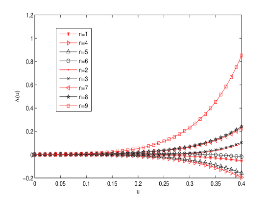
Figure 1: (color online) $\Lambda(u)$ vs. $u$ for the case of $N=2$ and $\{\theta_{j}=0\}$. The curves calculated from $T-Q$ relation (5.6) and the nested BAEs (5.14)-(5.15) are exactly the same as those obtained from the exact diagonalization of the transfer matrix $t(u)$.

6 Diagonal boundary case

When the parameters $c,c_{1},c_{2},c^{\prime},c_{1}^{\prime},c_{2}^{\prime}$ in the reflection matrices $K^{\pm}(u)$ given by (2.52) and (2.61) vanish, the corresponding $K$-matrices become diagonal ones. Let us denote them by $\bar{K}^{\pm}(u)$, namely,

$$\bar{K}^{-}(u)=\left(\begin{array}[]{ccc}e^{u}\sinh(\zeta-u)&0&0\\[6.0pt] 0&e^{u}\sinh(\zeta-u)&\\[6.0pt] 0&&e^{-u}\sinh(\zeta+u)\end{array}\right),$$ (6.4)

$$\bar{K}^{+}(u)={\cal M}\bar{K}^{-}(-u-3\eta/2)\left|{}_{\zeta\rightarrow\zeta^{\prime}}\right..$$ (6.5)

Moreover, the corresponding decomposition $\{K^{(i)}(u)\}$ in (5.16)-(5.18), if denoted by $\bar{K}^{(i)}(u)$, are given by

$$\bar{K}^{(1)}(u)=e^{\frac{3}{2}\eta}\sinh(\zeta+u)\sinh(\zeta^{\prime}-u+\frac{\eta}{2}),$$ (6.6)

$$\bar{K}^{(2)}(u)=e^{\frac{3}{2}\eta}\sinh(\zeta-u-\eta)\sinh(\zeta^{\prime}+u+\frac{3\eta}{2}),$$ (6.7)

$$\bar{K}^{(3)}(u)=\bar{K}^{(2)}(u).$$ (6.8)

Then the corresponding $T-Q$ relations (5.6)-(5.7) become the usual homogeneous ones and now are given by

$$\Lambda(u) = \frac{\sinh(2u+3\eta)}{\sinh(2u+\eta)}\bar{K}^{(1)}(u)a_{0}(u)\frac{\bar{Q}^{(1)}(u-\eta)}{\bar{Q}^{(1)}(u)}$$ (6.9)

$$\,+\frac{\sinh 2u\sinh(2u+3\eta)}{\sinh(2u+\eta)\sinh(2u+2\eta)}\bar{K}^{(2)}(u)b_{0}(u)\frac{\bar{Q}^{(1)}(u+\eta)\bar{Q}^{(2)}(u-\eta)}{\bar{Q}^{(1)}(u)\bar{Q}^{(2)}(u)}$$

$$\,+\frac{\sinh 2u}{\sinh(2u+2\eta)}\bar{K}^{(3)}(u)b_{0}(u)\frac{\bar{Q}^{(2)}(u+\eta)}{\bar{Q}^{(2)}(u)},$$

$$\Lambda_{2}(u) = \rho_{2}(2u-\eta)b_{0}(u-\eta)$$ (6.10)

$$\times\left\{\frac{\sinh(2u-2\eta)\sinh(2u+3\eta)}{\sinh 2u\sinh(2u-\eta)}\bar{K}^{(1)}(u)\bar{K}^{(2)}(u-\eta)a_{0}(u)\frac{\bar{Q}^{(2)}(u-2\eta)}{\bar{Q}^{(2)}(u-\eta)}\right.$$

$$\,\left.+\frac{\sinh(2u-2\eta)\sinh(2u+3\eta)}{\sinh(2u+\eta)\sinh 2u}\bar{K}^{(1)}(u)\bar{K}^{(3)}(u-\eta)a_{0}(u)\frac{\bar{Q}^{(1)}(u-\eta)\bar{Q}^{(2)}(u)}{\bar{Q}^{(1)}(u)\bar{Q}^{(2)}(u-\eta)}\right.$$

$$\,+\left.\frac{\sinh(2u-2\eta)\sinh(2u+3\eta)}{\sinh(2u+\eta)\sinh(2u+2\eta)}\bar{K}^{(2)}(u)\bar{K}^{(3)}(u-\eta)b_{0}(u)\frac{\bar{Q}^{(1)}(u+\eta)}{\bar{Q}^{(1)}(u)}\right\}.$$

Here the corresponding $Q$-functions are

$$\bar{Q}^{(k)}(u)=\prod_{l=1}^{\bar{M}_{k}}\sinh(u-\lambda^{(k)}_{l})\sinh(u+\lambda^{(k)}_{l}+k\eta),\quad 0\leq\bar{M}_{2}\leq N,\quad 0\leq\bar{M}_{1}\leq\bar{M}_{2}.$$ (6.11)

The resulting homogeneous relation (6.9) recovers that obtained by the algebraic Bethe ansatz method [52], while the reference state is chosen as

$$|vac>=\left(\begin{array}[]{c}0\\ 0\\ 1\end{array}\right)\otimes\left(\begin{array}[]{c}0\\ 0\\ 1\end{array}\right)\otimes\left(\begin{array}[]{c}0\\ 0\\ 1\end{array}\right)\otimes\cdots\otimes\left(\begin{array}[]{c}0\\ 0\\ 1\end{array}\right),$$ (6.24)

and the associated creation operators are the off-diagonal matrix elements of the 3-rd row of the double-row monodromy matrix $\mathbb{T}(u)$ given by (2.64).

7 Conclusions

In this paper, we study the exact solution of the anisotropic quantum spin chain with generic open boundary conditions and associated with $SU_{q}(3)$ algebra. After giving the off-diagonal reflection matrixes, by using the fusion technique, we obtain some closed operator identities among the transfer matrices, the degenerate points and the corresponding asymptotic behaviors. Based on them, we construct the nested inhomogeneous $T-Q$ relations and the Bethe ansatz equations. These results can be generalized to the higher rank case. Moreover, when the boundary parameters take special values corresponding to the diagonal reflection matrices, our results recover those previously obtained by the conventional Bethe ansatzs.

Appendix: Asymptotic behaviors for the other two cases reflecting matrices

When the reflection matrices $K^{\pm}$ are given by (2.56) and (2.61), the asymptotic behaviors of fused transfer matrices $t_{m}(u)$ are

$$t_{1}(u)|_{u\rightarrow+\infty} = -\frac{1}{4^{N+1}}e^{(2N+4)u+3\eta}\left[c^{\prime}\frac{c_{1}c_{2}}{c}e^{2\eta}\,e^{2\eta{\cal{Q}}^{(2)}}\right.$$ (A.1)

$$+\left.(c_{1}c_{2}^{\prime}+c_{1}^{\prime}c_{2}e^{4\eta})e^{N\eta}e^{-\eta{\cal{Q}}^{(2)}}\right]+\cdots,$$

$$t_{1}(u)|_{u\rightarrow-\infty} = -\frac{1}{4^{N+1}}e^{-(2N+4)u-3\eta}\left[c\frac{c_{1}^{\prime}c_{2}^{\prime}}{c^{\prime}}e^{2\eta}\,e^{-2\eta{\cal{Q}}^{(2)}}\right.$$ (A.2)

$$\left.+(c_{1}c_{2}^{\prime}+c_{1}^{\prime}c_{2}e^{4\eta})\,e^{-N\eta}\,e^{\eta{\cal{Q}}^{(2)}}\right]+\cdots,$$

$$t_{2}(u)|_{u\rightarrow+\infty} = -\frac{1}{4^{2N+3}}e^{4(N+3)u+5\eta}c^{\prime}\frac{c_{1}c_{2}}{c}\left[c\frac{c_{1}^{\prime}c_{2}^{\prime}}{c^{\prime}}e^{2\eta}\,e^{-2\eta{\cal{Q}}^{(2)}}\right.$$ (A.3)

$$\left.+(c_{1}c_{2}^{\prime}+c_{1}^{\prime}c_{2}e^{4\eta})e^{-N\eta}\,e^{\eta{\cal{Q}}^{(2)}}\right]+\cdots,$$

$$t_{2}(u)|_{u\rightarrow-\infty} = -\frac{1}{4^{2N+3}}e^{-4(N+3)u-\eta}c\frac{c_{1}^{\prime}c_{2}^{\prime}}{c^{\prime}}\left[c^{\prime}\frac{c_{1}c_{2}}{c}e^{2\eta}e^{2\eta{\cal{Q}}^{(2)}}\right.$$ (A.4)

$$\left.+(c_{1}c_{2}^{\prime}+c_{1}^{\prime}c_{2}e^{4\eta})\,e^{N\eta}\,e^{-\eta{\cal{Q}}^{(2)}}\right]+\cdots,$$

where the operator ${\cal{Q}}^{(2)}$ is

$${\cal{Q}}^{(2)}=\sum_{l=1}^{N}E^{22}_{l},\quad E^{22}=\left(\begin{array}[]{ccc}0&0&0\\ 0&1&0\\ 0&0&0\end{array}\right).$$ (A.8)

The asymptotic behaviors of fused transfer matrices $t_{m}(u)$ associated with the reflection matrices $K^{\pm}$ given by (2.60) and (2.61) are

$$t_{1}(u)|_{u\rightarrow+\infty} = -\frac{1}{4^{N+1}}e^{(2N+4)u+5\eta}\left[c^{\prime}\frac{c_{1}c_{2}}{c}e^{\eta}e^{2\eta{\cal{Q}}^{(3)}}\right.$$ (A.9)

$$\left.+(c_{1}c_{2}^{\prime}+c_{1}^{\prime}c_{2}e^{2\eta})\,e^{N\eta}\,e^{-\eta{\cal{Q}}^{(3)}}\right]+\cdots,$$

$$t_{1}(u)|_{u\rightarrow-\infty} = -\frac{1}{4^{N+1}}e^{-(2N+4)u-\eta}\left[c\frac{c_{1}^{\prime}c_{2}^{\prime}}{c^{\prime}}e^{\eta}e^{-2\eta{\cal{Q}}^{(3)}}\right.$$ (A.10)

$$\left.+(c_{1}c_{2}^{\prime}+c_{1}^{\prime}c_{2}e^{2\eta})\,e^{-N\eta}\,e^{\eta{\cal{Q}}^{(3)}}\right]+\cdots,$$

$$t_{2}(u)|_{u\rightarrow+\infty} = -\frac{1}{4^{2N+3}}e^{4(N+3)u+8\eta}c^{\prime}\frac{c_{1}c_{2}}{c}\left[c\frac{c_{1}^{\prime}c_{2}^{\prime}}{c^{\prime}}e^{\eta}\,e^{-2\eta{\cal{Q}}^{(3)}}\right.$$ (A.11)

$$\left.+(c_{1}c_{2}^{\prime}+c_{1}^{\prime}c_{2}e^{2\eta})\,e^{-N\eta}\,e^{\eta{\cal{Q}}^{(3)}}\right]+\cdots,$$

$$t_{2}(u)|_{u\rightarrow-\infty} = -\frac{1}{4^{2N+3}}e^{-4(N+3)u+2\eta}c\frac{c_{1}^{\prime}c_{2}^{\prime}}{c^{\prime}}\left[c^{\prime}\frac{c_{1}c_{2}}{c}e^{\eta}\,e^{2\eta{\cal{Q}}^{(3)}}\right.$$ (A.12)

$$\left.+(c_{1}c_{2}^{\prime}+c_{1}^{\prime}c_{2}e^{2\eta})\,e^{N\eta}\,e^{-\eta{\cal{Q}}^{(3)}}\right]+\cdots,$$

where the operator ${\cal{Q}}^{(3)}$ is

$${\cal{Q}}^{(3)}=\sum_{l=1}^{N}E^{33}_{l},\quad E^{33}=\left(\begin{array}[]{ccc}0&0&0\\ 0&0&0\\ 0&0&1\end{array}\right).$$ (A.16)

Some remarks are in order. Similarly as the operator ${\cal{Q}}^{(1)}$ given by (3.35), the above operator ${\cal{Q}}^{(2)}$ (resp. ${\cal{Q}}^{(3)}$) generates a remaining $U(1)$-symmetry for the corresponding model respectively. Moreover the eigenvalues of the operator are $0,\,1,\cdots,N$. Hence the whole Hilbert space can be decomposed into the subspaces labeled by its eigenvalue, on which the transfer matrices are invariant. We can calculate the asymptotic behaviors of the corresponding transfer matrices on each subspace.

For the reflection matrix $K^{\pm}$ given by (2.56) and (2.61), the asymptotic behaviors of $\Lambda_{m}(u)$ can be obtained by acting the operator (A.1)-(A.4) on the subspace on which the eigenvalue of the operator ${\cal{Q}}^{(2)}$ is $M$. After some calculations, we arrive at

$$\Lambda_{1}(u)|_{u\rightarrow+\infty} = -\frac{e^{(2N+4)u+3\eta}}{4^{N+1}}\left[c^{\prime}\frac{c_{1}c_{2}}{c}e^{2M\eta+2\eta}+(c_{1}c_{2}^{\prime}+c_{1}^{\prime}c_{2}e^{4\eta})e^{(N-M)\eta}\right]+\cdots,$$ (A.17)

$$\Lambda_{1}(u)|_{u\rightarrow-\infty} = -\frac{1}{4^{N+1}}e^{-(2N+4)u-3\eta}\left[c\frac{c_{1}^{\prime}c_{2}^{\prime}}{c^{\prime}}e^{-2M\eta+2\eta}\right.$$ (A.18)

$$\left.+(c_{1}c_{2}^{\prime}+c_{1}^{\prime}c_{2}e^{4\eta})e^{(M-N)\eta}\right]+\cdots,$$

$$\Lambda_{2}(u)|_{u\rightarrow+\infty} = -\frac{1}{4^{2N+3}}e^{4(N+3)u+5\eta}c^{\prime}\frac{c_{1}c_{2}}{c}\left[c\frac{c_{1}^{\prime}c_{2}^{\prime}}{c^{\prime}}e^{-2M\eta+2\eta}\right.$$ (A.19)

$$\left.+(c_{1}c_{2}^{\prime}+c_{1}^{\prime}c_{2}e^{4\eta})e^{(M-N)\eta}\right]+\cdots,$$

$$\Lambda_{2}(u)|_{u\rightarrow-\infty} = -\frac{1}{4^{2N+3}}e^{-4(N+3)u-\eta}c\frac{c_{1}^{\prime}c_{2}^{\prime}}{c^{\prime}}\left[c^{\prime}\frac{c_{1}c_{2}}{c}e^{2M\eta+2\eta}\right.$$ (A.20)

$$\left.+(c_{1}c_{2}^{\prime}+c_{1}^{\prime}c_{2}e^{4\eta})e^{(N-M)\eta}\right]+\cdots.$$

For the reflection matrix $K^{\pm}$ given by (2.60) and (2.61), the asymptotic behaviors of $\Lambda_{m}(u)$ can be obtained by acting the operator (A.9)-(A.12) on the subspace on which the eigenvalue of the operator ${\cal{Q}}^{(3)}$ is $M$. The finial results read

$$\Lambda_{1}(u)|_{u\rightarrow+\infty} = -\frac{e^{(2N+4)u+5\eta}}{4^{N+1}}\left[c^{\prime}\frac{c_{1}c_{2}}{c}e^{2M\eta+\eta}+(c_{1}c_{2}^{\prime}+c_{1}^{\prime}c_{2}e^{2\eta})e^{(N-M)\eta}\right]+\cdots,$$ (A.21)

$$\Lambda_{1}(u)|_{u\rightarrow-\infty} = -\frac{1}{4^{N+1}}e^{-(2N+4)u-\eta}\left[c\frac{c_{1}^{\prime}c_{2}^{\prime}}{c^{\prime}}e^{-2M\eta+\eta}\right.$$ (A.22)

$$\left.+(c_{1}c_{2}^{\prime}+c_{1}^{\prime}c_{2}e^{2\eta})e^{(M-N)\eta}\right]+\cdots,$$

$$\Lambda_{2}(u)|_{u\rightarrow+\infty} = -\frac{1}{4^{2N+3}}e^{4(N+3)u+8\eta}c^{\prime}\frac{c_{1}c_{2}}{c}\left[c\frac{c_{1}^{\prime}c_{2}^{\prime}}{c^{\prime}}e^{-2M\eta+\eta}\right.$$ (A.23)

$$\left.+(c_{1}c_{2}^{\prime}+c_{1}^{\prime}c_{2}e^{2\eta})e^{(M-N)\eta}\right]+\cdots,$$

$$\Lambda_{2}(u)|_{u\rightarrow-\infty} = -\frac{1}{4^{2N+3}}e^{-4(N+3)u+2\eta}c\frac{c_{1}^{\prime}c_{2}^{\prime}}{c^{\prime}}\left[c^{\prime}\frac{c_{1}c_{2}}{c}e^{2M\eta+\eta}\right.$$ (A.24)

$$\left.+(c_{1}c_{2}^{\prime}+c_{1}^{\prime}c_{2}e^{2\eta})e^{(N-M)\eta}\right]+\cdots.$$

For the reflection matrix $K^{\pm}$ given by (2.56) and (2.61), the eigenvalues of the transfer matrices $t(u)$ and $t_{2}(u)$ are described by the ansatz (5.6) and (5.7) with the decomposition

$$K^{(1)}(u)=e^{2\eta}(e^{-u}\sinh(\zeta+u)-c\sinh 2u)$$

$$\hskip 56.9055pt\times(e^{u-\frac{\eta}{2}}\sinh(\zeta^{\prime}-u+\frac{\eta}{2})+c^{\prime}\sinh 2(u-\frac{\eta}{2})),$$ (A.25)

$$K^{(2)}(u)=e^{2\eta}(e^{u+\eta}\sinh(\zeta-u-\eta)+c\sinh 2(u+\eta))$$

$$\hskip 56.9055pt\times(e^{-u-\frac{3\eta}{2}}\sinh(\zeta^{\prime}+u+\frac{3\eta}{2})-c^{\prime}\sinh 2(u+\frac{3\eta}{2})),$$ (A.26)

$$K^{(3)}(u)=K^{(2)}(u),$$ (A.27)

and the parameter $h$ takes the value of

$$h=c\frac{c_{1}^{\prime}c_{2}^{\prime}}{c^{\prime}}e^{-(M+N)\eta-12\eta}+c^{\prime}\frac{c_{1}c_{2}}{c}e^{(M+N)\eta+16\eta}-(c_{1}c_{2}^{\prime}+c_{1}^{\prime}c_{2}e^{4\eta}).$$ (A.28)

For the reflection matrix $K^{\pm}$ given by (2.60) and (2.61), the eigenvalues of the transfer matrices $t(u)$ and $t_{2}(u)$ are also characterized by the ansatz (5.6) and (5.7) with the parametrization

$$K^{(1)}(u)=e^{2\eta}(e^{u}\sinh(\zeta-u)-ce^{2u}\sinh 2u)$$

$$\hskip 56.9055pt\times(e^{-u+\frac{\eta}{2}}\sinh(\zeta^{\prime}+u-\frac{\eta}{2})+c^{\prime}e^{-2(u-\frac{\eta}{2})}\sinh 2(u-\frac{\eta}{2})),$$ (A.29)

$$K^{(2)}(u)=e^{2\eta}(e^{-u-\eta}\sinh(\zeta+u+\eta)+ce^{-2(u+\eta))}\sinh 2(u+\eta))$$

$$\hskip 56.9055pt\times(e^{u+\frac{3\eta}{2}}\sinh(\zeta^{\prime}-u-\frac{3\eta}{2})-c^{\prime}e^{2(u+\frac{3\eta}{2})}\sinh 2(u+\frac{3\eta}{2})),$$ (A.30)

$$K^{(3)}(u)=K^{(2)}(u),$$ (A.31)

and the constant $h$ is given by

$$h=c\frac{c_{1}^{\prime}c_{2}^{\prime}}{c^{\prime}}e^{-(M+N)\eta-11\eta}+c^{\prime}\frac{c_{1}c_{2}}{c}e^{(M+N)\eta+17\eta}-(c_{1}c_{2}^{\prime}+c_{1}^{\prime}c_{2}e^{2\eta})e^{2\eta}.$$ (A.32)

References

- [1] R.J. Baxter, Exactly Solved Models in Statistical Mechanics, Academic Press, 1982.
- [2] V.E. Korepin, N. M. Bogoliubov and A. G. Izergin, Quantum Inverse Scattering Method and Correlation Function, Cambridge University Press, 1993.
-
[3]
R.J. Baxter, Phys. Rev. Lett. 26 (1971) 832;
R.J. Baxter, Phys. Rev. Lett. 26 (1971) 834;
R.J. Baxter, Ann. Phys. 70 (1967) 323. - [4] L.A. Takhtadzhan and L. D. Faddeev, Rush. Math. Surveys 34 (1979) 11.
- [5] E.K. Sklyanin and L.D. Faddeev, Sov. Phys. Dokl. 23 (1978) 902.
- [6] F.C. Alcaraz, M.N. Barber, M.T. Batchelor, R.J. Baxter and G.R.W. Quispel, J. Phys. A 20 (1987) 6397.
- [7] E.K. Sklyanin, J. Phys. A 21 (1988) 2375.
- [8] J. Cao, W.-L. Yang, K. Shi and Y. Wang, Phys. Rev. Lett. 111 (2013) 137201.
- [9] J. Cao, H.-Q. Lin, K.-J. Shi and Y. Wang, Nucl. Phys. B 663 (2003) 487.
-
[10]
J. de Gier and P. Pyatov, J. Stat. Mech.
(2004) P03002;
A. Nichols, V. Rittenberg and J. de Gier, J. Stat. Mech. (2005) P03003;
J. de Gier, A. Nichols, P. Pyatov and V. Rittenberg, Nucl. Phys. B 729 (2005) 387. -
[11]
J. de Gier and F.H.L. Essler, Phys.
Rev. Lett. 95 (2005) 240601;
J. de Gier and F.H.L. Essler, J. Stat. Mech. (2006) P12011. - [12] Z. Bajnok, J. Stat. Mech. (2006) P06010.
- [13] P. Baseilhac, Nucl. Phys. B 754 (2006) 309.
- [14] P. Baseilhac and K. Koizumi, J. Stat. Mech. (2007) P09006.
-
[15]
P. Baseilhac and S. Belliard, Lett. Math. Phys. 93 (2010)
213;
P. Baseilhac and S. Belliard, Nucl. Phys. B 873 (2013) 550. - [16] S. Belliard and N. Crampé, SIGMA 9 (2013) 072.
- [17] S. Belliard, Nucl. Phys. B 892 (2015) 1.
- [18] S. Belliard and R.A. Pimenta, Nucl. Phys. B 894 (2015) 527.
- [19] J. Avan, S. Belliard, N. Grosjean and R.A. Pimenta, Nucl. Phys. B 899 (2015) 229.
-
[20]
E.K. Sklyanin, Lecture Notes in Physics 226 (1985) 196;
E.K. Sklyanin, J. Sov. Math. 31 (1985) 3417;
E.K. Sklyanin, Prog. Theor. Phys. Suppl. 118 (1995) 35. - [21] H. Frahm, A. Seel and T. Wirth, Nucl. Phys. B 802 (2008) 351.
-
[22]
G. Niccoli, Nucl. Phys. B 870 (2013) 397;
G. Niccoli, J. Phys. A 46 (2013) 075003. - [23] S. Faldella, N. Kitanine and G. Niccoli, J. Stat. Mech. (2014) P01011.
- [24] N. Kitanine, J.-M. Maillet and G. Niccoli, J. Stat. Mech. (2014) P05015.
-
[25]
R.I. Nepomechie, J. Phys. A 34
(2001) 9993;
R.I. Nepomechie, Nucl. Phys. B 622 (2002) 615;
R.I. Nepomechie, J. Stat. Phys. 111 (2003) 1363;
R.I. Nepomechie, J. Phys. A 37 (2004) 433. -
[26]
W.-L. Yang and Y.-Z. Zhang, J. High Energy Phys. 12 (2004) 019;
W.-L. Yang and Y.-Z. Zhang, J. High Energy Phys. 01 (2005) 021. -
[27]
A. Doikou and P.P. Martins, J. Stat. Mech. (2006)
P06004;
A. Doikou, J. Stat. Mech. (2006) P09010. - [28] W.-L. Yang, R.I. Nepomechie and Y.-Z. Zhang, Phys. Lett. B 633 (2006) 664.
- [29] R.I. Nepomechie, J. Phys. A 46 (2013) 442002.
- [30] J. Cao, W.-L. Yang, K. Shi and Y. Wang, Nucl. Phys. B 875 (2013) 152.
- [31] J. Cao, S. Cui, W.-L. Yang, K. Shi and Y. Wang, Nucl. Phys. B 886 (2014) 185.
- [32] J. Cao, W.-L. Yang, K. Shi and Y. Wang, Nucl. Phys. B 877 (2013) 152.
- [33] J. Cao, W.-L. Yang, K. Shi and Y. Wang, J. High Energy Phys. 04 (2014) 143.
- [34] Y.-Y. Li, J. Cao, W.-L. Yang, K. Shi and Y. Wang, Nucl. Phys. B 884 (2014) 17.
- [35] X. Zhang, J. Cao, W.-L. Yang, K. Shi and Y. Wang, J. Stat. Mech. (2014) P04031.
- [36] K. Hao, J. Cao, G.-L. Li, W.-L. Yang, K. Shi and Y. Wang, J. High Energy Phys. 06 (2014) 128.
- [37] Y. Wang, W.-L. Yang, J. Cao and K. Shi, Off-Diagonal Bethe Ansatz for Exactly Solvable Models, Springer Press, 2015.
- [38] J.H.H. Perk and C.L. Schultz, Phys. Lett. A 84 (1981) 407.
- [39] J.H.H. Perk and C.L. Schultz, Families of commuting transfer matrices in q-state vertex models, in Non-linear integrable systems - classical theory and quantum theory, eds. M. Jimbo and T. Miwa, World Scientific, 1983, pp. 135-152.
- [40] C.L. Schultz, Physica A 122 (1983) 71.
- [41] J.H. H. Perk and H. Au-Yang, Yang-Baxter Equation, in Encyclopedia of Mathematical Physics, eds. J.-P. Françoise, G.L. Naber and T.S. Tsun, Academic Press, 2006.
- [42] V.V. Bazhanov, Phys. Lett. B 159 (1985) 321.
- [43] M. Jimbo, Commun. Math. Phys. 102 (1986) 537.
- [44] A. Lima-Santos, Nucl. Phys. B 558 (1999) 637.
- [45] K. Shi, G. -L. Li, H. Fan and B. Y. Hou, High Energy Phys. and Nucl. Phys. 24 (2000) 11.
- [46] R. Malara and A. Lima-Santos, J. Stat. Mech. (2006) P09013.
-
[47]
M. Karowski, Nucl. Phys. B 153 (1979) 244;
P.P. Kulish, N.Yu. Reshetikhin and E.K. Sklyanin, Lett. Math. Phys. 5 (1981) 393;
P.P. Kulish and E.K. Sklyanin, Lecture Notes in Physics 151 (1982) 61;
A.N. Kirillov and N.Yu. Reshetikhin, J. Sov. Math. 35 (1986) 2627;
A.N. Kirillov and N.Yu. Reshetikhin, J. Phys. A 20 (1987) 1565. - [48] L. Mezincescu and R.I. Nepomechie, Nucl. Phys. B 372 (1992) 597.
- [49] Y.-K. Zhou, Nucl. Phys. B 458 (1996) 504.
- [50] H.J. de Vega and A. Gonzlez-Ruiz, Nucl. Phys. B 417 (1994) 553.
- [51] H.J. de Vega and A. Gonzlez-Ruiz, Mod. Phys. Lett. A 09 (1994) 2207.
- [52] G.-L. Li, R. H. Yue and B. Y. Hou, Nucl. Phys. B 586 (2000) 711.