Adaptation Logic for HTTP Dynamic Adaptive Streaming using Geo-Predictive Crowdsourcing

Abstract

The increasing demand for video streaming services with high Quality of Experience (QoE) has prompted a lot of research on client-side adaptation logic approaches. However, most algorithms use the client’s previous download experience and do not use a crowd knowledge database generated by users of a professional service. We propose a new crowd algorithm that maximizes the QoE. Additionally, we show how crowd information can be integrated into existing algorithms and illustrate this with two state-of-the-art algorithms. We evaluate our algorithm and state-of-the-art algorithms (including our modified algorithms) on a large, real-life crowdsourcing dataset that contains 336,551 samples on network performance. The dataset was provided by WeFi LTD. Our new algorithm outperforms all other methods in terms of QoS (eMOS).

I Introduction

Dynamic Adaptive Streaming over HTTP (DASH) [1] is the HTTP Adaptive Streaming (HAS) standard. It has been recently adopted by YouTube (Google) and Netflix. DASH splits a video into chunks and encodes each into several quality representations.

A client’s DASH application often has a smart Adaptation Logic (AL) module. The AL module is responsible for selecting the most suitable quality representation to enhance the client’s Quality of Experience (QoE) while considering factors such as the client’s buffer and playback delay. QoE is affected by factors such as the number of quality changes and their sizes.

There is a tradeoff between increasing the video quality and buffering additional video segments. A client’s player often buffers a high number of segments to overcome network outages.

Most of the current AL methods [2, 3, 4, 5, 6, 7, 8, 9, 10], estimate the next suitable segment based on estimates of previous segments without taking into account the future network characteristics. However, knowledge of geo-location network conditions can enable better decisions.

The term crowdsourcing was introduced by Howe [11]. Howe defined crowdsourcing as the act of taking a task traditionally performed by a designated agent (such as an employee or a contractor) and outsourcing it by making an open call to an undefined but large group of people, especially from an online community.

In the case of video adaptive streaming, crowdsourcing makes it possible to collect mobile network data anonymously and automatically. This is done using an application specially designed to improve the AL decision. Neidhardt et al. [12] reports that using many of the existing open datasets leads to low accuracy because of extreme outliers and few measurements for some of the cells. They note that cellular location providers do not provide their complete data. In this work, we present a real-world crowdsourcing dataset and test our proposed solution based on different users.

We propose a Geo-Predictive Adaptive Logic (GPAL) algorithm based on crowdsourcing data on network performance provided by WeFi. WeFi collects granular information on mobile network performance and application usage from millions of devices, down to a $10\times 10$ meter geographical resolution. A short 20-record sample of these data can be found in [13].

We dub our new crowd algorithm GPAL and show that it outperforms state-of-the-art algorithms. Moreover, we show that existing adaptation algorithms can be improved by using crowd services. However, our algorithm outperforms these algorithms even in this scenario. It is worth noting that our crowd sourcing data was generated by users of a professional service and not by a simulation.

The remainder of this paper is organized as follows: Section II describes related work. Section III presents our proposed crowd algorithms. Section IV present our dataset characteristics. Section V presents the experimental setup and results. Section VI discusses future work and conclusions.

II Related Work

DASH AL is a well-investigated research topic. AL research can be roughly divided into two different groups: past estimation based AL and crowdsourcing based AL. Most work has investigated past estimation algorithms.

Müller et al. [8] suggested a buffer based decision algorithm that uses the previous segment bandwidth estimates and the user’s current buffer duration to select a suitable quality representation for downloading. The Multicast Adaptation Logic (MAL) algorithm [10] uses a double Exponential Moving Average (EMA) algorithm. One smooths the buffer size estimate and the other smooths the bandwidth estimate. This is done to select the most suitable segment. Although MAL was designed for multicast, it achieves good performance in unicast networks [10].

Crowdsourcing AL methods have attracted much less attention than past estimation based methods. Hung et al. [14] proposed a video streaming control mechanism based on location to overcome signal variations in train tunnels and underground areas. Geo-location frameworks that have the ability to predict future network conditions based on a bandwidth lookup service and similar concepts can be found in [15, 16, 17, 18, 19]. Acharya et al.[20] evaluated rate-adaptation in a vehicular network based on signal strength and throughput at a location as an indicator for congestion. Curcio et al. [15] and Singh et al. [16] suggested server-side prediction algorithms for RTP streaming. Curcio et al. [15] suggested a framework with a predictive server which obtains: route, speed, location and throughput from the client. However, this study was based on simulation rather than real-world data. Singh et al. [16] proposed building a Network Coverage Map Service (NCMS) to make rate-control decisions over a Real Time Protocol (RTP) using server-side adaptation algorithm. Singh et al. however did not investigate performance on datasets with a higher geographical coverage or more diverse network connectivity conditions.

Yao et al. [17] showed that past bandwidth information is a good indicator of the actual bandwidth at a given location. Yao et al. found that location had greater influence than time, based on traces. Nevertheless, their performance evaluation did not take into account the number of switches or the playout buffer size. Furthermore, it was gathered from a small set of vehicles.

Riiser et al. [18] proposed a buffer based and a crowd-based algorithm. Riiser et al. concluded that using past bandwidth lookups led to far fewer rebuffering events and stabler quality. Han et al. [21] investigated the extent to which the available user mobile channel bandwidth is affected by constraints including location, time, speed, humidity and cellular network type (3G/4G). Their scheme, called MASERATI, outperformed Pure-DASH and LoDASH, where Pure-DASH only uses the download throughput and LoDASH uses location based bandwidth predictions as in [22, 18].

Liu et al. [23] suggested comparing the segment fetch time with the media duration contained in the segment to detect congestion and probe the spare network capacity. Liu’s algorithm uses conservative step-wise up switching and aggressive down switching. Hao et al.[19] suggested two algorithms: 1-predict and n-predict. The 1-predict algorithm uses the playout buffer and the next prediction to determine the most suitable representation to download. The n-predict algorithm uses the average throughput of the next n time steps as the algorithm’s current prediction. Hao et al. [19] evaluated Liu et al.’s algorithm and found that it achieved stable video quality but with a very low average bitrate. They showed that n-predict outperformed Liu et al’s algorithm as well as 1-predict .

Zou et al. [24] demonstrated that leveraging bandwidth predictions can significantly improve QoE. They designed an algorithm that combines bitrate prediction and rate stabilization. They showed that during startup, their algorithm had more than four times better video quality than heuristic-based algorithms.

Riiser et al. [25] recorded $3G$ mobile traces in Oslo, Norway, while traveling in different types of public transportation (metro, tram, train, bus and ferry). However, the number of contributors in the dataset was small.

Table I summarizes the papers presented above.

TABLE I: Comparison of Algorithms

Paper	Streaming Protocol	Idea	Trigger	Action	Quality Adjustment	Compared Algorithms	Observed Metrics	Mobility Simulate
Singh et el. [16] - Geo-location Assisted Streaming System (GLASS) Rate-Switching	RTP/UDP + Temporal Maximum Media Stream Bit rate Request (TMMBR)	Avoiding buffer underrun - client looks ahead at locations in its vicinity for bad coverage	Future Coverage Hole	Client Pre-Buffer	Client media rate switch according to available throughput in the coverage hole	No adaptation (RTCP), rate switching GLASS, late scheduling GLASS, Omniscient (Optimal)	packet loss rate, average receive rate, Y component of the PSNR, throughput	Actual specific bandwidth trace
Yao et al. [17] - BW-MAP-TFRC	adaptive TCP streaming with TCP Friendly Rate Control (TFRC) [26]	Avoiding packet loss - client updates the server when it changes its location. The server determines the average bandwidth at that location in the past	Location changed by client followed by a new BW value	Server changes its sending rate	Short freezing of the TFRC and disabling the normal operation of TFRC when needed	TFRC and BW-MAP-TFRC	estimated Mean Opinion Score [27], Peak Signal-to-Noise Ratio (PSNR), Glitch (Drop in the streaming quality)	Actual specific bandwidth trace
Riiser et al. [18]	Apple Live HTTP	Minimizing rapid fluctuations in quality and avoiding buffer underrun - client’s estimate of the number of bytes that it can download during the remaining time of the trip	Client receives a sequence of bandwidth averages for its whole path	Client plans which quality levels to use	Apple Live HTTP mechanism	Buffer-Based Reactive, History-Based Prediction, Omniscient Prediction (Optimal)	Buffer size, selected representations	Actual specific bandwidth trace
Han et al. [21] - MASERATI	DASH	Avoiding frequent or large video quality changes	The algorithm finds the most similar database entry and estimates the available bandwidth	The bit rate of the next video segment is defined by that bandwidth	DASH Adaptation mechanism	Pure-DASH, Location-based DASH (LoDASH) [18], MASERATI	Playout Success Rate, Quality of Segments, Frequency of Quality Changes, Degree of Changed Quality Level	Actual specific bandwidth trace
Hao et al.[19] - 1-predict, n-predict	DASH	Achieving continuous playback - DASH Based algorithm with an additional function to anticipate future path and bandwidth, and to determine the predicted rate	The server calculates the possible bandwidth and sends it to the client	DASH Client applies the best quality level it can afford	DASH Adaptation mechanism	Liu et al. [23], Adobes Open Source Media Framework (OSMF), 1-Predict, N-Predict	Segment representation Level, Ratio of bandwidth utilization, rate of video quality level shift	Actual specific bandwidth trace
Zou et al. [24] - PBA	DASH	Avoiding stalls, preserving stability while maintaining improved average quality - the client decides which quality to pick using the buffer state and the quality of historical chunks	Buffer occupancy changes all the time during download	Client can decide when to download and quality level	DASH	FESTIVE [28] , BBA [29], optimal( mixed integer linear programing), PBA	Average quality rate supplied in the first 360s/32s, Number of stalls, Number of switches	Actual specific bandwidth trace

III Proposed Geo-Predictive Algorithms

We define the user playout buffer as $B(t)$. The goal of the AL modules is to maximize the overall quality of the stream, while eliminating rebuffering ($B(t)>0$). We measure the quality in terms of its eMOS score [30] as shown in Eq. 1.

$$\begin{split}\max(\text{eMOS})\;\;\;&s.t:\\ \forall t>t_{start}\;\;0<B(t)&\leq B_{max}\end{split}$$ (1)

We first show how to integrate crowd information to existing algorithms. This is done by estimating the bandwidth. The estimate is based on the crowd and not on the network. We demonstrate the approach with two state-of-the-art algorithms, MAL (Section III-A) and MaxBW (Section III-B).

We also present a novel Geo-Predictive Adaptation Logic (GPAL) algorithm that is designed to maximize the QoE (Section III-C).

Our crowd bandwidth estimation algorithm is presented in Algorithm 1. This algorithm was used for GPAL, Geo-MaxBW and Geo-MAL.

Algorithm 1 Geo predictive bandwidth estimation algorithm, used by GPAL, Geo-MaxBW and Geo-MAL.

1:g: current mobile geo-location.

2:v: current mobile speed.

3:w: highest quality average file size.

4:f: last downloaded segment throughput estimate.

5:radius: search radius.

6:$X_{bw}(t)$: bandwidth estimate for the current time ($t$).

7:estimate: g,v

8:seg  =  $\frac{\textsl{v}\textsl{w}}{\textsl{f}}$

9:$X_{bw}(t)$   =  getCrowdPrediction(radius, g, seg)

III-A Geo-MAL

Dubin et al. [10] showed that using a Double Exponential Moving Average (DEMA) estimator achieved good results in unicast and multicast networks. Based on these results, we present a new Geo-predictive MAL algorithm using a crowdsource adapted DEMA estimator (Eqs. 2-3). The full algorithm is presented in Algorithm 2.

The DEMA estimator uses a parameter to balance the influence of the current measurement vs. the influence of the previous estimate on the current estimate. Increasing the parameter increases the weight of the current measurement and decreases the weight of the previous estimate. In MAL [10], they used $\alpha$ to denote the parameter used for the client’s buffer estimate and $\beta$ to denote the parameter used for the channel bandwidth estimate. One of the main challenges is to choose appropriate values for $\alpha$ and $\beta$ to best comply with the requirements of Eq. 1. Similar to [10] we used $\alpha=0.2$ and $\beta=0.08$. We define $S_{b}(t)$ as the smoothed buffer estimate and $S_{bw}(t)$ as the smoothed bandwidth estimation:

$$\begin{split}S_{b}(0)&=B(0)\\ \forall t>0\;\;S_{b}(t)&=(\alpha)B(t)+(1-\alpha)S_{b}(t-1)\\ \end{split}$$ (2)

$$\begin{split}S_{bw}(0)&=X_{bw}(0)\\ \forall t>0\;\;S_{bw}(t)&=(\beta)X_{bw}(t)+(1-\beta)S_{bw}(t-1)\\ \end{split}$$ (3)

Algorithm 2 Geo-MAL: Geo Predictive MAL Algorithm

1:critical: playout buffer contains 2 segments.

2:low: playout buffer contains 4 segments.

3:$B_{max}$: maximum buffer size.

4:almost full: playout buffer contains $B_{max}-2$ segments.

5:safety factor: 0.5.

6:Estimate $X_{bw}(t)$ for each segment download.

7:if start or re-buffering then

8:     if next representation$<$estimated bandwidth $\cdot$ safety factor then

9:         Ask for the highest representation available under that condition

10:     end if

11:end if

12:if segment is received then

13:     if  (buffer is depleting) and
aaaaa ((buffer level $\leq$ critical) or
aaaaaaa ((buffer level $\leq$ low) and (estimated bandwidth $<$ current representation bitrate))) then

14:         Switch down

15:     else if  (next representation bitrate $<$ estimated bandwidth) and
aaaaa (( buffer level $\geq$ almost full ) or
aaaaaaa (buffer level is safe and is filling)) then

16:         Switch up

17:     end if

18:end if

III-B Geo-MaxBW Adaptation Logic

The MaxBW algorithm [2] adaptive decision is based on the measured download time of each segment and the average measured bitrate of the whole session. The Geo-MaxBW algorithm uses a crowd-based bandwidth estimate as presented in Algorithm 1.

III-C Geo-Predictive Adaptation Logic (GPAL)

The GPAL algorithm, Algorithm 3, determines the representation of the next media segment to be fetched. The algorithm estimates the current segment download path based on the client’s location and speed. It predicts the future path network bandwidth conditions based on the client’s playout buffer and the crowd estimated throughput. The algorithm calculates the playout buffer fullness ratio ($B_{p}$) based on the maximum between the current buffer levels divided by the maximum buffer size allocation and 10%. We used the 10% to select a higher bandwidth when the playout buffer is drained.

Algorithm 3 GPAL: Geo Predictive Adaptation Logic Algorithm

1:$\rho$: predicted mobile bandwidth for next segment.

2:$B(t)$: current playout buffer duration.

3:$B_{p}$: playout buffer fullness ratio.

4:$B_{max}$: maximum buffer size.

5:$\tau$: selected quality for download.

6:$B_{p}=\frac{B(t)}{B_{max}}$

7:if first segment then

8:     $B_{p}$ = 0.5

9:end if

10:Estimate $X_{bw}(t)$ for each segment download.

11:$\rho$ = $X_{bw}(t)\cdot B_{p}$

12:$\tau$ = the highest bit rate representation for which $\tau<\rho$

13:if $B_{p}$ = 0.2 then

14:     Reduce $\tau$ in one representation.

15:end if

16:return $\tau$

IV Dataset

The WeFi dataset contains $336,551$ samples from the California I110 and I405 interstates. The I110 is an interstate highway in the Los Angeles area and connects San Pedro and the port of Los Angeles with downtown Los Angeles and Pasadena. The I405 is a major north-south interstate highway in Southern California. Table II summarizes the interstates’ general features.

	I110	I405
Date of creation	$1-7.12.2014$	$1-7.12.2014$
Number of samples	$125079$	$211472$
Section length	$30$ $km$	$17$ $km$
Number of users	$5838$	$6170$
Number of samples	$125079$	$211472$

TABLE II: Interstate roads summary

A large number of different applications generated the data. Most of the applications either regularly send low rate updates or are in the idle state (sending keep-alive messages).

We estimate the average throughput (bits per second) per sample $s$ for the interval $x$ using Eq 4.

$$\begin{split}E_{x}=\frac{\sum_{s\in x}D_{s}\cdot A_{s}}{\sum_{s\in x}D_{s}}\\ \end{split}$$ (4)

where $D_{s}$ is the total data received in sample $s$ and $A_{s}$ is the average throughput in sample $s$. Figs 1-2 illustrate the average throughput per sample for an interval ($E_{x}$) vs. the throughput ($A_{s}$). In these figures, each path is divided into $12$ meter segments.

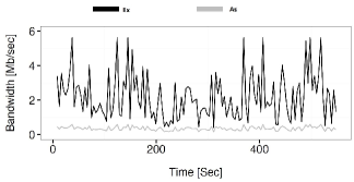
Figure 1: I110 average throughput per sample for an interval ($E_{x}$) vs. the throughput ($A_{s}$)

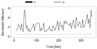
Figure 2: I405 average throughput per sample for an interval ($E_{x}$) vs. the throughput ($A_{s}$)

IV-A Interstate I110

The interstate heat map is illustrated in Fig. 3(a) which shows that the road throughput can vary between $0.5-5[Mb/s]$. Fig. 3(b) depicts the measured bandwidth of the path (average and STD). We define this bandwidth path as I110.

The median throughput of the interstate is $0.86[Mb/s]$, the average throughput is $1.585[Mb/s]$ and the STD is $2$. That is, the path has many fluctuations. Thus, it is challenging for adaptive streaming clients to adapt to its network conditions.

Fig. 3(c) depicts the throughput density and the sample densities along the route. We split the throughput density into fixed bins from $0$ to the maximum observed throughput, $10[Mb/s]$. It is clear that lower throughput in the ranges of $0-2[Mb/s]$ are more likely while throughput above $5[Mb/s]$ are less common. Fig. 3(d) shows the sample densities along the route. From $23km$ the sample densities decrease. Figs. 3(e) - 3(h) show the throughput behavior in different time ranges. Obviously, the demand for bandwidth at night (21:00 - 3:00) is much lower than during rush hour. Table. III summarizes the average bit rate at different time periods.

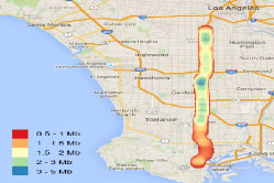
(a) I110 throughput heat map.

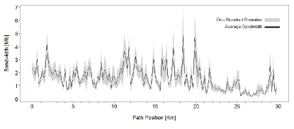
(b) I110 path positioning

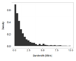
(c) Bandwidth entropy (PMF) analysis

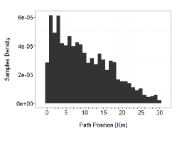
(d) Samples density entropy (PMF) analysis

(e) Route average throughput between 3:00 - 9:00

(f) Route average throughput between 9:00 - 15:00

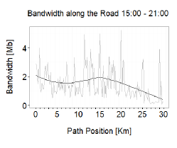
(g) Route average throughput between 15:00 - 21:00

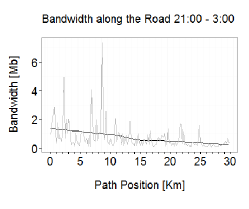
(h) Route average throughput between 21:00 - 03:00

Figure 3: Interstate I110 dataset detailed depiction.

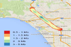
(a) I405 throughput heat map.

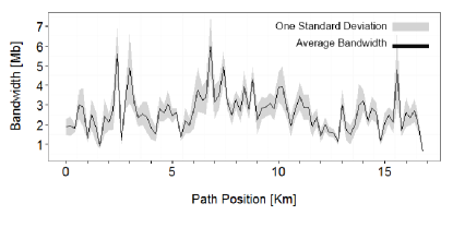
(b) I405 path positioning

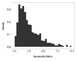
(c) Bandwidth entropy (PMF) analysis

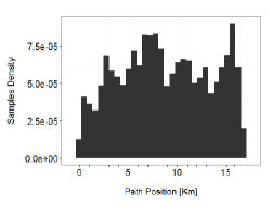
(d) Samples density entropy (PMF) analysis

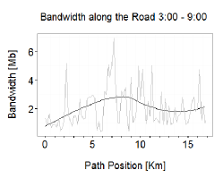
(e) Route’s throughput average between 3:00 - 9:00

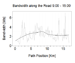
(f) Route’s throughput average between 9:00 - 15:00

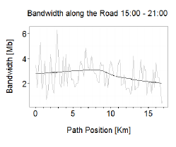
(g) Route’s throughput average between 15:00 - 21:00

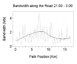
(h) Route’s throughput average between 21:00 - 3:00

Figure 4: Interstate I405 dataset detailed depiction.

Time range	Average bit rate [Mb/s]
3:00-9:00	$1.6$
9:00-15:00	$1.24$
15:00-21:00	$1.46$
21:00-3:00	$0.72$

TABLE III: Interstate I110 average bit rate at different hours

IV-B Interstate I405

The I405 interstate is shorter but has a higher number of samples than the I110 interstate (see Table II). The interstate heat map is illustrated in Fig. 4(a) which shows that the road throughput varies between $0.5-5[Mb/s]$. Fig. 4(b) depicts the measured bandwidth of the path (average and STD). We define this bandwidth path as $I405A$.

The median throughput of the interstate is $1.97[Mb/s]$, the average throughput is $2.63[Mb/s]$ and the STD is $2.15$. The I405 interstate has a higher throughput average than I110. The STD is slightly higher.

Fig. 4(c) illustrates the throughput density and the sample densities along the route. We split the throughput density into fixed bins from $0$ to the maximum observed throughput $10[Mb/s]$. The table shows that the I405 throughput density is different from the I110 throughput density and the throughput is better spread between $0.5-2.5[Mb/s]$. Fig. 4(d) depicts the density of the samples along the route. This road is more evenly dense than I110. Figs. 4(e) - 4(h) show the throughput behavior at different time periods. It shows that the throughput demand on this road is higher even in the late hours (Fig. 4(h)).

V Experiments and Results

We describe our experimental setup and video representation information in Section V-A. We discuss our experimental results Sections V-B, V-C and V-D.

V-A Experimental Setup

This section describes our experimental settings and video encoding configuration. We used the Big Buck Bunny (BBB) [31] video encoded into fixed duration segments of $2$ seconds. Table IV illustrates the BBB available representation stored in the streaming server. The client playout buffer duration was set to $30$ seconds.

Representation	SSIM	PSNR $[dB]$	Average bit rate $[Kb/s]$
$50$	$0.719$	$24.4$	$51.05$
$100$	$0.8$	$28.3$	$98.91$
$200$	$0.89$	$32.4$	$193.31$
$250$	$0.914$	$34$	$240.96$
$500$	$0.96$	$38$	$480.15$
$750$	$0.971$	$40$	$721.56$
$1000$	$0.977$	$41.4$	$964.16$
$1500$	$0.985$	$0.91$	$1452.44$
$2000$	$0.988$	$44.5$	$1942.4$
$2400$	$0.989$	$45.28$	$2335.2041$

TABLE IV: Big Buck Bunny representation information

Fig. 5 illustrates our experimental setup. First, the user requests (VLC [32]) the video MPD file from the HTTP server. After the client receives it, the adaptation logic algorithm requests the crowd estimate from the PostgreSQL geo-predictive server. Then, the user sends a request to the server using a simple API implementation which only sends the following information to the server: the search radius ($250$ meters), the user’s current location and the estimated end point (which depends on the user’s average speed). The geo-predictive module predicts the average throughput. Since this API is very lightweight, the process delay is negligible. We do not assume we know the route. Therefore, we used a batch fetching mechanism. That is, before the current segment download ends, we fetch the crowd estimate for the next segment. Each adaptation logic can analyze the data or use the API differently but the fetching optimization is beyond the scope of this study. The DumyNet [33] shapes the traffic according to the network scenario. As a result, the segment download is delayed according to the network conditions. In order to compare our work to state-of-the-art algorithms we used the same segment fetching schema as these works, where the client downloads each segment one after the other.

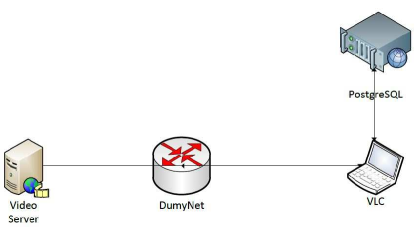
Figure 5: Experimental setup diagram

V-B Experimental Results

In Eq. 1 we stated our goal. In our experiments $B_{max}$ was 30 seconds. All compared algorithms realized the constraints of Eq. 1 (as can be seen in Figs. 6-7). Table V summarizes the average eMOS score [30] for all the algorithms. The table shows that our GPAL algorithm outperforms all other algorithms. Additionally, the integration of crowd information into state-of-the-art algorithms boosts their performance. Geo-MaxBW eMOS score was $4.35$ whereas the non-crowd-based MaxBW eMOS score was only $4.21$. Similarly, Geo-MAL eMOS score was $3.74$ whereas the non-crowd-based MAL eMOS score was only $3.41$.

Algorithm	Avergae eMOS
GPAL (our, Section III-C)	$4.39$
MaxBW ([2])	$4.21$
Geo-MaxBW (our adaptation of [2], Section III-B)	$4.35$
MAL ([2])	$3.41$
Geo-MAL (our adaptation of [10], Section III-A)	$3.74$
1-Predict ([19])	$3.24$
n-Predict ([19])	$2.15$
PBA ([24])	$2.89$
MASERATI ([21])	$1.37$

TABLE V: Average eMOS score for all algorithms

V-C Detailed Results of Interstate I110 and Discussion

In this section we present the experimental results for Interstate I110. Fig.6 presents the bandwidth estimate, the downloaded bitrate and the buffer estimate.

Fig. 6(b) shows that MaxBW had a relatively high bandwidth. Nevertheless, the algorithm selected the suitable representation. MaxBW does not constrain the number of representation switches. As a result, the algorithm had the highest number of quality switches ($187$). MaxBW achieved the highest eMOS score compared to all non-crowd algorithms without any re-buffering events (see Table V). It is noteworthy that the eMOS score includes factors such as the number of switch events and re-buffering events.

Fig. 6(d) shows that MAL smoothed most of the small bit rate variations and gave restrained bandwidth estimates that translated into a low number of quality switches ($33$). It did so without any prior knowledge about the path network conditions. Note that the algorithm adjusted too late to the decreasing channel throughput ($150-200$ seconds). When the channel bitrate decreased even further, the algorithm failed to recognize it and encountered $4$ short re-buffering events.

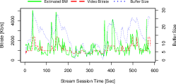
(a) GPAL

(b) MaxBW

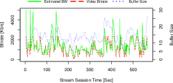
(c) Geo-MaxBW

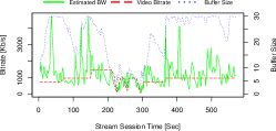
(d) MAL

(e) Geo-MAL

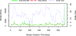
(f) 1-Predict

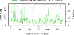
(g) n-Predict

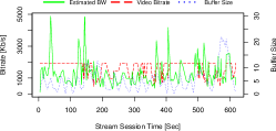
(h) PBA

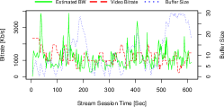
(i) MASERATI

Figure 6: Algorithms’ bandwidth and buffer estimates with the selected video bitrate for the Interstate I110 path.

Hao et al.[19] suggested two algorithms: 1-predict and n-predict. Their goal was to put forward a crowd-based algorithm with fewer representation switches that could also minimize re-buffering events. Fig. 6(f) shows that 1-predict’s bit rate estimates was relatively high. Even though the number of representation switches was high ($95$) the algorithm maintained a balanced playout buffer and downloaded high quality segments without re-buffering events. The n-predict algorithm achieved very different results compared to the 1-predict algorithm. Fig. 6(g) shows that the n-predict algorithm had the lowest number of representation switches and that the playout buffers were extremely high. But the n-predict algorithm tended to select lower representations; thus, its eMOS score is the lowest (see Table V).

The Prediction Based Adaptation (PBA) [24] algorithm considers the buffer occupancy based on three buffer thresholds and aggressively tries to stabilize rate selection. Fig. 6(h) shows that the algorithm tried to stay in the same representation but the buffer occupancy tended to fluctuate which caused serious re-buffering events.

The MASERATI algorithm uses a weighted average which considers the past estimates and the adjusted bandwidth from the crowd database. Fig. 6(i) shows that there was a relatively high number of representation switches ($82$) whereas the total re-buffering duration was $39$ seconds. For a crowd algorithm the average estimated throughput was low compared to other crowd algorithms.

The Geo-MAL algorithm increased the number of representation switches and minimized the number of re-buffering events. Fig. 6(e) and Table. V show that Geo-MAL improved the MAL eMOS score by $9.6\%$ without any re-buffering events. The MAL algorithm was designed for multicast networks. Thus, its throughput estimates are low and it tends to download lower representations. It tends to smooth the network’s fluctuations and thus its bandwidth estimates are relatively low.

The Geo-MaxBW (Fig. 6(c)) crowd adaptation replaces the MaxBW’s previous segment throughput estimate with the crowd throughput estimate. The result was a slight reduction in the number of representation switches and the average eMOS score increased by $3.3\%$.

Our GPAL algorithm is a buffer based approach inspired by the MaxBW algorithm combined with crowd knowledge. Fig. 6(a) shows that the algorithm utilized the crowd in the most effective way and yielded an average throughput estimate of $1.3[Mb/s]$ compared to the other crowd algorithms that generated lower utilization. GPAL had a relatively low number of representation switches ($48\%$). Table V shows that the algorithm had the best average eMOS score.

V-D Interstate I405 Results

Interstate I405 (see Fig. 4) differs from Interstate I110 and its bandwidth is spread better in the path. This caused the algorithms to select different representations than for I110. Fig. 7 shows that the MAL algorithm, which is an exponential moving average based algorithm, smooths the bandwidth estimate. Surprisingly, compared to I110 the algorithm did not have re-buffering events, but this time Geo-MAL did. MAL based algorithms do not check whether the estimated throughput or crowd throughput are lower than the selected representation. This behavior led to re-buffering. The MaxBW algorithm exhibited good performance, similar to I110. However the number of representation switches increased to $130$. The Geo-MaxBW reduced the number of representation switches to $28$. The other algorithms’ behavior was similar to I110. Table V shows that the average eMOS score for MaxBW gave the best result for non-crowd algorithms whereas GPAL outperformed all the other algorithms.

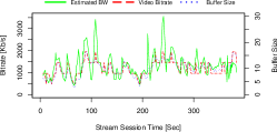
(a) GPAL

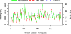
(b) MaxBW

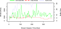
(c) Geo-MaxBW

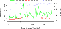
(d) MAL

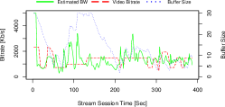
(e) Geo-MAL

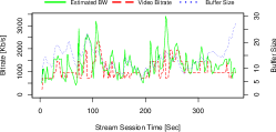
(f) 1-Predict

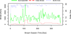
(g) n-Predict

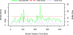
(h) PBA

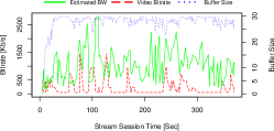
(i) MASERATI

Figure 7: Algorithms’ bandwidth and buffer estimates with the selected video bitrate for the Interstate I405 path.

VI Conclusion

We showed that the use of real-world crowd data can improve existing algorithms and demonstrated it on two different algorithms: Geo-MAL and Geo-MaxBW. Geo-MAL presented a $9.6\%$ average eMOS score improvement over MAL whereas Geo-MaxBW had a $3.3\%$ improvement over MaxBW. We proposed a new crowd-based algorithm called GPAL that outperformed all other state-of-the-art algorithms. We conclude that an optimal adaptation logic should estimate the distance between the current conditions and the cloud conditions. Our future work will aim to design an adaptation algorithm that can leverage the advantages of past download algorithms with crowd knowledge based on the conclusions drawn from this work. An interesting approach would be to implement machine learning algorithms (similar to Claeys et al. [30]) combined with crowd data. An additional interesting research direction would be to harness a client-side pre-fetch and $HTTP2$ server-side push mechanism based on crowd knowledge.

References

- [1] ISO/IEC. Information technology - Dynamic adaptive streaming over HTTP (DASH), May 2014.
- [2] C. Müller, S. Lederer, and C. Timmerer. An evaluation of dynamic adaptive streaming over http in vehicular environments. In Proceedings of the 4th Workshop on Mobile Video, pages 37–42, Feb. 2012.
- [3] R. K. P. Mok, X. Luo E. W. W. Chan, and R. K. C. Chang. Qdash: a qoe-aware dash system. In Proceedings of the 3rd Multimedia Systems Conference, pages 11–22. ACM, 2012.
- [4] R. Dubin, O. Hadar, and A. Dvir. The effect of client buffer and mbr consideration on dash adaptation logic. In WCNC, pages 2178–2183, 2013.
- [5] Tingyao T. Wu and W. Leekwijck. Factor selection for reinforcement learning in http adaptive streaming. In MultiMedia Modeling, volume 8325 of Lecture Notes in Computer Science, pages 553–567. Springer International Publishing, 2014.
- [6] C. Mueller, S. Lederer, and C. Timmerer. A proxy effect analysis and fair adaptation algorithm for multiple competing dynamic adaptive streaming over http clients. In Proceedings of the IEEE Conference on Visual Communications and Image Processing Conference (VCIP 2012); IEEE, Piscataway (NJ), page 6 pages, November 2012.
- [7] L. De Cicco, V. Caldaralo, V. Palmisano, and S. Mascolo. Elastic: a client-side controller for dynamic adaptive streaming over http (dash). In Packet Video Workshop (PV), 2013 20th International, pages 1–8. IEEE, 2013.
- [8] C. Müller, S. Lederer, and C. Timmerer. An evaluation of dynamic adaptive streaming over http in vehicular environments. In Proceedings of the 4th Workshop on Mobile Video, pages 37–42. ACM, 2012.
- [9] R. Dubin, O. Hadar, B. Ben-Moshe, and A. Dvir. A novel adaptive logic for dynamic adaptive streaming over http network. In IEEEI, 2014.
- [10] R. Dubin, A. Dvir, O. Hadar, N. Harel, and R. Barkan. Multicast adaptive logic for dynamic adaptive streaming over http network. In Workshop Communication and Networking Techniques for Contemporary Video (INFOCOM workshop), 2015.
- [11] Jeff Howe. Crowdsourcing: Why the power of the crowd is driving the future of business. Journal of Consumer Marketing, 26(4):305–306, 2009.
- [12] E. Neidhardt, A. Uzun, U. Bareth, and A. Kupper. Estimating locations and coverage areas of mobile network cells based on crowdsourced data. In Wireless and Mobile Networking Conference (WMNC), 2013 6th Joint IFIP, pages 1–8. IEEE, 2013.
- [13] WeFi LTD. Wefi data set: for full sample please contact wefi at alexander at wefi dot com. https://goo.gl/QVi54N.
- [14] CM. Huang, SW. Wu, and YT. Yu. Lbvs-t: A location-based video streaming control scheme for trains. In Wireless and Mobile Computing, Networking and Communications (WiMob), 2014 IEEE 10th International Conference on, pages 679–684. IEEE, 2014.
- [15] IDD. Curcioa nd VKM. Vadakital and MM. Hannuksela. Geo-predictive real-time media delivery in mobile environment. In Proceedings of the 3rd workshop on Mobile video delivery, pages 3–8. ACM, 2010.
- [16] V. Singh, J. Ott, and IDD. Curcio. Predictive buffering for streaming video in 3g networks. In World of Wireless, Mobile and Multimedia Networks (WoWMoM), 2012 IEEE International Symposium on a, pages 1–10. IEEE, 2012.
- [17] J. Yao, SS. Kanhere, and M. Hassan. Improving qos in high-speed mobility using bandwidth maps. Mobile Computing, IEEE Transactions on, 11(4):603–617, 2012.
- [18] H. Riiser, T. Endestad, P. Vigmostad, C. Griwodz, and P. Halvorsen. Video streaming using a location-based bandwidth-lookup service for bitrate planning. ACM Transactions on Multimedia Computing, Communications, and Applications (TOMCCAP), 8(3):24, 2012.
- [19] J. Hao, R. Zimmermann, and H. Ma. Gtube: geo-predictive video streaming over http in mobile environments. In Proceedings of the 5th ACM Multimedia Systems Conference, pages 259–270. ACM, 2014.
- [20] PAK. Acharya, A. Sharma, EM. Belding, KC. Almeroth, and K. Papagiannaki. Congestion-aware rate adaptation in wireless networks: A measurement-driven approach. In Sensor, Mesh and Ad Hoc Communications and Networks, 2008. SECON’08. 5th Annual IEEE Communications Society Conference on, pages 1–9. IEEE, 2008.
- [21] D. Han, J. Han, Y. Im, M. Kwak, TT. Kwon, and Y. Choi. Maserati: mobile adaptive streaming based on environmental and contextual information. In Proceedings of the 8th ACM international workshop on Wireless network testbeds, experimental evaluation & characterization, pages 33–40. ACM, 2013.
- [22] K. Evensen, A. Petlund, H. Riiser, P. Vigmostad, D. Kaspar, C. Griwodz, and P. Halvorsen. Mobile video streaming using location-based network prediction and transparent handover. In International Workshop on Network and Operating Systems Support for Digital Audio and Video (NOSSDAV), pages 21–26, 2011.
- [23] C. Liu, I. Bouazizi, and M. Gabbouj. Rate adaptation for adaptive http streaming. In ACM Multimedia Systems, pages 169–174, CA, USA, Feb. 2011.
- [24] X. K. Zou, J. Erman, V. Gopalakrishnan, E. Halepovic, R. Jana, X. Jin, J. Rexford, and R. K. Sinha. Can Accurate Predictions Improve Video Streaming in Cellular Networks? In Proceedings of the 16th International Workshop on Mobile Computing Systems and Applications, HotMobile ’15, pages 57–62, 2015.
- [25] H. Riiser, P. Vigmostad, C. Griwodz, and P. Halvorsen. Commute path bandwidth traces from 3g networks: analysis and applications. In Proceedings of the 4th ACM Multimedia Systems Conference, pages 114–118. ACM, 2013.
- [26] M. Handley, S. Floyd, J. Padhye, and J. Widmer. Tcp friendly rate control (tfrc): Protocol specification. Technical report, 2002.
- [27] ITUT SG12. The e-model, a computational model for use in transmission planning. Recommendation G, 107, 2005.
- [28] J. Jiang, V. Sekar, and H. Zhang. Improving fairness, efficiency, and stability in http-based adaptive video streaming with festive. In Proceedings of the 8th international conference on Emerging networking experiments and technologies, pages 97–108. ACM, 2012.
- [29] TY. Huang, R. Johari, N. McKeown, M. Trunnell, and M. Watson. A buffer-based approach to rate adaptation: Evidence from a large video streaming service. In Proceedings of the 2014 ACM conference on SIGCOMM, pages 187–198. ACM, 2014.
- [30] M. Claeys, S. Latré, J. Famaey, T. Wu, W. Van Leekwijck, and F. De Turck. Design and optimisation of a (fa) q-learning-based http adaptive streaming client. Connection Science, 26(1):25–43, 2014.
- [31] Big Buck Bunny video. http://www.bigbuckbunny.org/, 2008.
- [32] C. Müller and C. Timmerer. A vlc media player plugin enabling dynamic adaptive streaming over http. In ACM Multimedia, pages 723–726, Arizona, USA, Nov. 2011.
- [33] M. Carbone and L. Rizzo. Dummynet. Website, 2010. http://info.iet.unipi.it/~luigi/dummynet/.