Compressive Spectral Clustering

Abstract

Spectral clustering has become a popular technique due to its high performance in many contexts. It comprises three main steps: create a similarity graph between $N$ objects to cluster, compute the first $k$ eigenvectors of its Laplacian matrix to define a feature vector for each object, and run $k$-means on these features to separate objects into $k$ classes. Each of these three steps becomes computationally intensive for large $N$ and/or $k$. We propose to speed up the last two steps based on recent results in the emerging field of graph signal processing: graph filtering of random signals, and random sampling of bandlimited graph signals. We prove that our method, with a gain in computation time that can reach several orders of magnitude, is in fact an approximation of spectral clustering, for which we are able to control the error. We test the performance of our method on artificial and real-world network data.

1 Introduction

Spectral clustering (SC) is a fundamental tool in data mining (Nascimento & de Carvalho, 2011). Given a set of $N$ data points $\{\bm{x}_{1},\ldots,\bm{x}_{N}\}$, the goal is to partition this set into $k$ weakly inter-connected clusters. Several spectral clustering algorithms exist, e.g., (Ng et al., 2002; Shi & Malik, 2000; Belkin & Niyogi, 2003; Zelnik-Manor & Perona, 2004), but all follow the same scheme. First, compute weights $\mathsf{W}_{ij}\geqslant 0$ that model the similarity between pairs of data points $(\bm{x}_{i},\bm{x}_{j})$. This gives rise to a graph $\mathcal{G}$ with $N$ nodes and adjacency matrix $\mathsf{W}=(\mathsf{W}_{ij})_{1\leqslant i,j\leqslant N}\in\mathbb{R}^{N\times N}$. Second, compute the first $k$ eigenvectors $\mathsf{U}_{k}:=(\bm{u}_{1},\ldots,\bm{u}_{k})\in\mathbb{R}^{N\times k}$ of the Laplacian matrix $\mathsf{L}\in\mathbb{R}^{N\times N}$ associated to $\mathcal{G}$ (see Sec. 2 for $\mathsf{L}$’s definition). And finally, run $k$-means using the rows of $\mathsf{U}_{k}$ as feature vectors to partition the $N$ data points into $k$ clusters. This $k$-way scheme is a generalisation of Fiedler’s pioneering work (1973).

SC is mainly used in two contexts: $1)$ if the $N$ data points show particular structures (e.g., concentric circles) for which naive $k$-means clustering fails; $2$) if the input data is directly a graph $\mathcal{G}$ modeling a network (White & Smyth, 2005), such as social, neuronal, or transportation networks. SC suffers nevertheless from three main computational bottlenecks for large $N$ and/or $k$: the creation of the similarity matrix $\mathsf{W}$; the partial eigendecomposition of the graph Laplacian matrix $\mathsf{L}$; and $k$-means.

1.1 Related work

Circumventing these bottlenecks has raised a significant interest in the past decade. Several authors have proposed ideas to tackle the eigendecomposition bottleneck, e.g., via the power method (Boutsidis & Gittens, 2015; Lin & Cohen, 2010), via a careful optimisation of diagonalisation algorithms in the context of SC (Liu et al., 2007), or via matrix column-subsampling such as in the Nyström method (Fowlkes et al., 2004), the nSPEC and cSPEC methods of (Wang et al., 2009), or in (Chen & Cai, 2011; Sakai & Imiya, 2009). All these methods aim to quickly compute feature vectors, but $k$-means is still applied on $N$ feature vectors. Other authors, inspired by research aiming at reducing k-means complexity (Jain, 2010), such as the line of work on coresets (Har-Peled & Mazumdar, 2004), have proposed to circumvent $k$-means in high dimension by subsampling a few data points out of the $N$ available ones, applying SC on its reduced similarity graph, and interpolating the results back on the complete dataset. One can find similar methods in (Yan et al., 2009) and (Wang et al., 2009)’s eSPEC proposition, where two different interpolation methods are used. Both methods are heuristic: there is no proof that these methods approach the results of SC. Also, let us mention (Dhillon et al., 2007) that circumvents both the eigendecomposition and the $k$-means bottlenecks: the authors reduce the graph’s size by successive aggregation of nodes, apply SC on this small graph, and propagate the results on the complete graph using kernel $k$-means to control interpolation errors. The kernel is computed so that kernel $k$-means and SC share the same objective function (Filippone et al., 2008). Finally, we mention works (Boutsidis et al., 2011; Cohen et al., 2015) that concentrate on reducing the feature vectors’ dimension in the $k$-means problem, but do not sidestep the eigendecomposition nor the large $N$ issues.

1.2 Contribution: compressive clustering

In this work, inspired by recent advances in the emerging field of graph signal processing (Shuman et al., 2013; Sandryhaila & Moura, 2014), we circumvent SC’s last two bottlenecks and detail a fast approximate spectral clustering method for large datasets, as well as the supporting theory. We suppose that the Laplacian matrix $\mathsf{L}\in\mathbb{R}^{N\times N}$ of $\mathcal{G}$ is given. Our method is made of two ingredients.

The first ingredient builds upon recent works (Tremblay et al., 2016; Ramasamy & Madhow, 2015) that avoid the costly computation of the eigenvectors of $\mathsf{L}$ by filtering $O(\log(k))$ random signals on $\mathcal{G}$ that will then serve as feature vectors to perform clustering. We show in this paper how to incorporate the effects of non-ideal, but computationally efficient, graph filters on the quality of the feature vectors used for clustering.

The second ingredient uses a recent sampling theory of bandlimited graph-signals (Puy et al., 2015) to reduce the computational complexity of $k$-means. Using the fact that the indicator vectors of each cluster are approximately bandlimited on $\mathcal{G}$, we prove that clustering a random subset of $O(k\log(k))$ nodes of $\mathcal{G}$ using random features vectors of size $O(\log(k))$ is sufficient to infer rapidly and accurately the cluster label of all $N$ nodes of the graph. Note that the complexity of $k$-means is reduced to $O(k^{2}\log^{2}(k))$ instead of $O(Nk^{2})$ for SC. One readily sees that this method scales easily to large datasets, as will be demonstrated on artifical and real-world datasets containing up to $N=10^{6}$ nodes.

The proposed compressive spectral clustering method can be summarised as follows:

• generate a feature vector for each node by filtering $O(\log(k))$ random Gaussian signals on $\mathcal{G}$;

• sample $O(k\log(k))$ nodes from the full set of nodes;

• cluster the reduced set of nodes;

• interpolate the cluster indicator vectors back to the complete graph.

2 Background

2.1 Graph signal processing

Let $\mathcal{G}=(\mathcal{V},\mathcal{E},\mathbf{W})$ be an undirected weighted graph with $\mathcal{V}$ the set of $N$ nodes, $\mathcal{E}$ the set of edges, and $\mathbf{W}$ the weighted adjacency matrix such that $W_{ij}=W_{ji}\geqslant 0$ is the weight of the edge between nodes $i$ and $j$.

The graph Fourier matrix. Consider the graph’s normalized Laplacian matrix $\mathsf{L}=\mathsf{I}-\mathsf{D}^{-1/2}\mathsf{W}\mathsf{D}^{-1/2}$ where $\mathsf{I}$ is the identity in dimension $N$, and $\mathsf{D}$ is diagonal with $\mathsf{D}_{ii}=\sum_{j\neq i}\mathsf{W}_{ij}$. $\mathsf{L}$ is real symmetric and positive semi-definite, therefore diagonalizable as $\mathsf{L}=\mathsf{U}\Lambda\mathsf{U}^{\intercal}$, where $\mathsf{U}:=\left(\bm{u}_{1}|\bm{u}_{2}|\dots|\bm{u}_{N}\right)\in\mathbb{R}^{N\times N}$ is the orthonormal basis of eigenvectors and $\mathsf{\Lambda}\in\mathbb{R}^{N\times N}$ the diagonal matrix containing its sorted eigenvalues : $0=\lambda_{1}\leqslant\dots\leqslant\lambda_{N}\leqslant 2$ (Chung, 1997). By analogy to the continuous Laplacian operator whose eigenfunctions are the classical Fourier modes and eigenvalues their squared frequencies, the columns of $\mathsf{U}$ are considered as the graph’s Fourier modes, and $\{\sqrt{\lambda_{l}}\}_{l}$ as its set of associated “frequencies” (Shuman et al., 2013). Other types of graph Fourier matrices have been proposed, e.g., (Sandryhaila & Moura, 2013), but in order to exhibit the link between graph signal processing and SC, the Laplacian-based Fourier matrix appears more natural.

Graph filtering. The graph Fourier transform $\hat{\bm{x}}$ of a signal $\bm{x}$ defined on the nodes of the graph (called a graph signal) reads: $\hat{\bm{x}}=\mathsf{U}^{\intercal}\bm{x}$. Given a continuous filter function $h$ defined on $[0,2]$, its associated graph filter operator $\mathsf{H}\in\mathbb{R}^{N\times N}$ is defined as $\mathsf{H}:=h(\mathsf{L})=\mathsf{U}h(\mathsf{\Lambda})\mathsf{U}^{\intercal}$, where $h(\mathsf{\Lambda}):=\mbox{diag}(h(\lambda_{1}),h(\lambda_{2}),\cdots,h(\lambda_{N}))$. The signal $\bm{x}$ filtered by $h$ is $\mathsf{H}\bm{x}$. In the following, we consider ideal low-pass filters, denoted by $h_{\lambda_{c}}$, that satisfy, for all $\lambda\in[0,2]$,

$$h_{\lambda_{c}}(\lambda)=1,\mbox{ if }\lambda\leqslant\lambda_{c},\;\mbox{ and }\;h_{\lambda_{c}}(\lambda)=0,\mbox{ if not.}$$ (1)

Denote by $\mathsf{H}_{\lambda_{c}}$ the graph filter operator associated to $h_{\lambda_{c}}$.

Fast graph filtering. To filter a signal by $h$ without diagonalizing $\mathsf{L}$, one may approximate $h$ by a polynomial $\tilde{h}$ of order $p$ satisfying $\tilde{h}(\lambda):=\sum_{l=0}^{p}\alpha_{l}\lambda^{l}\simeq h(\lambda)$ for all $\lambda\in[0,2]$, where $\alpha_{1},\ldots,\alpha_{p}\in\mathbb{R}$. In matrix form, we have $\mathsf{\tilde{H}}:=\tilde{h}(\mathsf{L})=\sum_{l=0}^{p}\alpha_{l}\mathsf{L}^{l}\simeq\mathsf{H}.$ Let us highlight that we never compute the potentially dense matrix $\mathsf{\tilde{H}}$ in practice. Indeed, we are only interested in the result of the filtering operation: $\mathsf{\tilde{H}}\bm{x}=\sum_{l=0}^{p}\alpha_{l}\mathsf{L}^{l}\bm{x}\approx\mathsf{H}\bm{x}$ for $\bm{x}\in\mathbb{R}^{N}$, obtainable with only $p$ successive matrix-vector multiplications with $L$. The computational complexity of filtering a signal is thus $O(p\#\mathcal{E})$, where $\#\mathcal{E}$ is the number of edges of $\mathcal{G}$.

Algorithm 1 Spectral Clustering (Ng et al., 2002)

  Input: The Laplacian matrix $\mathsf{L}$, the number of clusters $k$

  $\bm{1\cdot}$ Compute $\mathsf{U}_{k}\in\mathbb{R}^{N\times k}$, $\mathsf{L}$’s first $k$ eigenvectors: $\mathsf{U}_{k}=\left(\bm{u}_{1}|\bm{u}_{2}|\cdots|\bm{u}_{k}\right)$.

  $\bm{2\cdot}$ Form the matrix $\mathsf{Y}_{k}\in\mathbb{R}^{N\times k}$ from $\mathsf{U}_{k}$ by normalizing each of $\mathsf{U}_{k}$’s rows to unit length: $\left(\mathsf{Y}_{k}\right)_{ij}=\left(\mathsf{U}_{k}\right)_{ij}/\sqrt{\sum_{j=1}^{k}\mathsf{U}_{ij}^{2}}$.

  $\bm{3\cdot}$ Treat each node $i$ as a point in $\mathbb{R}^{k}$ by defining its feature vector $\bm{f}_{i}\in\mathbb{R}^{k}$ as the transposed $i$-th row of $\mathsf{Y}_{k}$:

$$\bm{f}_{i}:=\mathsf{Y}_{k}^{\intercal}\bm{\delta}_{i},$$

where $\delta_{i}(j)=1$ if $j=i$ and $0$ otherwise.

  $\bm{4\cdot}$ To obtain $k$ clusters, run $k$-means with the Euclidean distance:

$$D_{ij}:=\left\|\bm{f}_{i}-\bm{f}_{j}\right\|$$ (2)

2.2 Spectral clustering

We choose here Ng et al.’s method (2002) based on the normalized Laplacian as our standard SC method. The input is the adjacency matrix $\mathsf{W}$ representing the pairwise similarity of all the $N$ objects to cluster. After computing its Laplacian $\mathsf{L}$, follow Alg. 1 to find $k$ classes.

3 Principles of CSC

Compressive spectral clustering (CSC) circumvents two of SC’s bottlenecks, the partial diagonalisation of the Laplacian and the high-dimensional $k$-means, thanks to the following ideas.

1) Perform a controlled estimation $\tilde{D}_{ij}$ of the spectral clustering distance $D_{ij}$ (see Eq (2)), without partially diagonalizing the Laplacian, by fast filtering a few random signals with the polynomial approximation $\tilde{h}_{\lambda_{k}}$ of the ideal low pass filter $h_{\lambda_{k}}$ (see Eq. (1)). A theorem recently published independently by two teams (Tremblay et al., 2016; Ramasamy & Madhow, 2015) shows that this is possible when there is no normalisation step (step 2 in Alg. 1) and when the order $p$ of the polynomial approximation tends to infinity, i.e., when $\tilde{h}_{\lambda_{k}}=h_{\lambda_{k}}$. In Sec. 3.1, we provide a first extension of this theorem that takes into account normalisation. A complete extension that also takes into account the polynomial approximation error is presented in Sec. 4.2.

2) Run $k$-means on $n$ randomly selected feature vectors out of the $N$ available ones - thus clustering the corresponding $n$ nodes into $k$ groups - and interpolate the result back on the full graph. To guarantee robust reconstruction, we take advantage of our recent results on random sampling of $k$-bandlimited graph signals. In Sec. 3.2, we explain why these results are applicable to clustering and show that it is sufficient to sample $n=O(k\log{k})$ features only! Note that to cluster data into $k$ groups, one needs at least $k$ samples. This result is thus optimal up to the extra $\log{k}$ factor.

3.1 Ideal filtering of random signals

Definition 3.1 (Local cumulative coherence).

Given a graph $\mathcal{G}$, the local cumulative coherence of order $k$ at node $i$ is $v_{k}(i):=\left\|\mathsf{U}_{k}^{\intercal}\bm{\delta}_{i}\right\|=\sqrt{\sum_{j=1}^{k}\mathsf{U}_{ij}^{2}}$.

Let us define the diagonal matrix: $\mathsf{V}_{k}(i,i)=1/v_{k}(i)$. Note that we assume that $v_{k}(i)>0$. Indeed, in the pathologic cases where $v_{k}(i)=0$ for some nodes $i$, step 2 of the standard SC algorithm cannot be run either. Now, consider the matrix $\mathsf{R}=\left(\bm{r}_{1}|\bm{r}_{2}|\cdots|\bm{r}_{d}\right)\in\mathbb{R}^{N\times d}$ consisting of $d$ random signals $\bm{r}_{i}$, whose components are independent Bernouilli, Gaussian, or sparse (as in Theorem 1.1 of (Achlioptas, 2003)) random variables. To fix ideas in the following, we consider the components as independent random Gaussian variables of mean zero and variance $1/d$. Consider the coherence-normalized filtered version of $\mathsf{R}$, $\mathsf{V}_{k}\mathsf{H}_{\lambda_{k}}\mathsf{R}\in\mathbb{R}^{N\times d}$, and define node $i$’s new feature vector $\tilde{\bm{f}}_{i}\in\mathbb{R}^{d}$ as the transposed $i$-th line of this filtered matrix:

$$\tilde{\bm{f}}_{i}:=(\mathsf{V}_{k}\mathsf{H}_{\lambda_{k}}\mathsf{R})^{\intercal}\bm{\delta}_{i}.$$

The following theorem shows that, for large enough $d$,

$$\tilde{D}_{ij}:=\left\|\tilde{\bm{f}}_{i}-\tilde{\bm{f}}_{j}\right\|=\left\|(\mathsf{V}_{k}\mathsf{H}_{\lambda_{k}}\mathsf{R})^{\intercal}(\bm{\delta}_{i}-\bm{\delta}_{j})\right\|$$

is a good estimation of $D_{ij}$ with high probability.

Theorem 3.2.

Let $\epsilon\in]0,1]$ and $\beta>0$ be given. If $d$ is larger than

$$\frac{4+2\beta}{\epsilon^{2}/2-\epsilon^{3}/3}\log{N},$$

then with probability at least $1-N^{-\beta}$, we have

$$(1-\epsilon)D_{ij}\leqslant\tilde{D}_{ij}\leqslant(1+\epsilon)D_{ij}.$$

for all $(i,j)\in\{1,\ldots,N\}^{2}$.

The proof is provided in the supplementary material.

In Sec. 4.2, we generalize this result to the real-world case where the low-pass filter is approximated by a finite order polynomial; we also prove that, as announced in the introduction, one only needs $d=O(\log{k})$ features when using the downsampling scheme that we now detail.

3.2 Downsampling and interpolation

For $j=1,\ldots,k$, let us denote by $\bm{c}_{j}\in\mathbb{R}^{N}$ the ground-truth indicator vector of cluster $\mathcal{C}_{j}$, i.e.,

$$(\bm{c}_{j})_{i}:=\left\{\begin{array}[]{ll}1&\text{if }i\in\mathcal{C}_{j},\\ 0&\text{otherwise},\end{array}\right.\quad\forall i\in\{1,\ldots,N\}.$$

To estimate $\bm{c}_{j}$, one could run $k$-means on the $N$ feature vectors $\{\tilde{\bm{f}}_{1},\ldots,\tilde{\bm{f}}_{N}\}$ , as done in (Tremblay et al., 2016; Ramasamy & Madhow, 2015). Yet, this is still inefficient for large $N$. To reduce the computational cost further, we propose to run $k$-means on a small subset of $n$ feature vectors only. The goal is then to infer the labels of all $N$ nodes from the labels of the $n$ sampled nodes. To this end, we need 1) a low-dimensional model that captures the regularity of the vectors $\bm{c}_{j}$, 2) to make sure that enough information is preserved after sampling to be able to recover the vectors $\bm{c}_{j}$, and 3) an algorithm that rapidly and accurately estimates the vectors $\bm{c}_{j}$ by exploiting their regularity.

3.2.1 The low-dimensional model

For a simple regular (with nodes of same degree) graph of $k$ disconnected clusters, it is easy to check that $\{\bm{c}_{1},\ldots,\bm{c}_{k}\}$ form a set of orthogonal eigenvectors of $\mathsf{L}$ with eigenvalue $0$. All indicator vectors $\bm{c}_{j}$ therefore live in ${\rm span}{(\mathsf{U}_{k})}$. For general graphs, we assume that the indicator vectors $\bm{c}_{j}$ live close to ${\rm span}{(\mathsf{U}_{k})}$, i.e., the difference between any $\bm{c}_{j}$ and its orthogonal projection onto ${\rm span}(\mathsf{U}_{k})$ is small. Experiments in Section 5 will confirm that it is a good enough model to recover the cluster indicator vectors.

In graph signal processing words, one can say that $\bm{c}_{j}$ is approximately $k$-bandlimited, i.e., its $k$ first graph Fourier coefficients bear most of its energy. There has been recently a surge of interest around adapting classical sampling theorems to such bandlimited graph signals (Chen et al., 2015; Anis et al., 2015; Tsitsvero et al., 2015; Marques et al., 2015). We rely here on the random sampling strategy proposed in (Puy et al., 2015) to select a subset of $n$ nodes.

3.2.2 Sampling and interpolation

The subset of feature vectors is selected by drawing $n$ indices $\Omega:=\{\omega_{1},\ldots,\omega_{n}\}$ uniformly at random from $\{1,\ldots,N\}$ without replacement. Running $k$-means on the subset of features $\{\tilde{\bm{f}}_{\omega_{1}},\ldots,\tilde{\bm{f}}_{\omega_{n}}\}$ thus yields a clustering of the $n$ sampled nodes into $k$ clusters. We denote by $\bm{c}_{j}^{r}\in\mathbb{R}^{n}$ the resulting low-dimensional indicator vectors. Our goal is now to recover $\bm{c}_{j}$ from $\bm{c}_{j}^{r}$.

Consider that $k$-means is able to correctly identify $\bm{c}_{1},\ldots,\bm{c}_{k}\in\mathbb{R}^{N}$ using the original set of features $\{\bm{f}_{1},\ldots,\bm{f}_{N}\}$ with the SC algorithm (otherwise, CSC is doomed to fail from the start). Results in (Tremblay et al., 2016; Ramasamy & Madhow, 2015) show that $k$-means is also able to identify the clusters using the feature vectors $\{\tilde{\bm{f}}_{1},\ldots,\tilde{\bm{f}}_{N}\}$. This is explained theoretically by the fact that the distance between all pairs of feature vectors is preserved (see Theorem 3.2). Then, as choosing a subset $\{\tilde{\bm{f}}_{\omega_{1}},\ldots,\tilde{\bm{f}}_{\omega_{n}}\}$ of $\{\tilde{\bm{f}}_{1},\ldots,\tilde{\bm{f}}_{N}\}$ does not change the distance between the feature vectors, we can hope that $k$-means correctly clusters the $n$ sampled nodes, provided that each cluster is sufficiently sampled. Experiments in Sec. 5 will confirm this intuition. In this ideal situation, we have

$$\bm{c}_{j}^{r}=\mathsf{M}\,\bm{c}_{j},$$ (3)

where $\mathsf{M}\in\mathbb{R}^{n\times N}$ is the sampling matrix satisfying:

$$\mathsf{M}_{ij}:=\left\{\begin{array}[]{ll}1&\text{if }j=\omega_{i},\\ 0&\text{otherwise}.\end{array}\right.$$ (6)

To recover $\bm{c}_{j}$ from its $n$ observations $\bm{c}_{j}^{r}$, Puy et al. (2015) show that the solution to the optimisation problem

$$\min_{\bm{x}\in\mathbb{R}^{N}}\left\|\mathsf{M}\bm{x}-\bm{c}_{j}^{r}\right\|_{2}^{2}+\gamma\;\bm{x}^{\intercal}g(\mathsf{L})\bm{x},$$ (7)

is a faithful  estimation of $\bm{c}_{j}$, provided that $\bm{c}_{j}$ is close to ${\rm span}(\mathsf{U}_{k})$ and that $\mathsf{M}$ satisfies the restricted isometry property (discussed in the next subsection). In (7), $\gamma>0$ is a regularisation parameter and $g$ a positive non-decreasing polynomial function (see Section 2.1 for the definition of $g(\mathsf{L})$). This reconstruction scheme is proved to be robust to: 1) observation noise, i.e., to imperfect clustering of the $n$ nodes in our context; 2)  model errors, i.e., the indicator vectors do not need to be exactly in ${\rm span}{(\mathsf{U}_{k})}$ for the method to work. Also, the performance is shown to depend on the ratio $g(\lambda_{k})/g(\lambda_{k+1})$. The smaller it is, the better the reconstruction. To decrease this ratio, we decide to approximate the ideal high-pass filter $g_{\lambda_{k}}(\lambda)=1-h_{\lambda_{k}}(\lambda)$ for the reconstruction. Remark that this filter favors the recovery of signals living in ${\rm span}{(\mathsf{U}_{k})}$. The approximation $\tilde{g}_{\lambda_{k}}$ of $g_{\lambda_{k}}$ is obtained using a polynomial (as in Sec. 2.1), which permits us to find fast algorithms to solve (7).

3.2.3 How many features to sample?

We terminate this section by providing the theoretical number of features $n$ one needs to sample in order to make sure that the indicator vectors can be faithfully recovered. This number is driven by the following quantity.

Definition 3.3 (Global cumulative coherence).

The global cumulative coherence of order $k$ of the graph $\mathcal{G}$ is $\nu_{k}~{}:=~{}\sqrt{N}~{}\cdot~{}\max_{1\leqslant i\leqslant N}\left\{v_{k}(i)\right\}.$

It is shown in (Puy et al., 2015) that $\nu_{k}\in[k^{1/2},N^{1/2}]$.

Theorem 3.4 ((Puy et al., 2015)).

Let $\mathsf{M}$ be a random sampling matrix constructed as in (6). For any $\delta,\epsilon\in\;]0,1[$,

$$(1-\delta)\left\|\bm{x}\right\|_{2}^{2}\leqslant\frac{N}{n}\left\|\mathsf{M}\,\bm{x}\right\|_{2}^{2}\leqslant(1+\delta)\left\|\bm{x}\right\|_{2}^{2}$$ (8)

for all $\bm{x}\in{\rm span}(\mathsf{U}_{k})$ with probability at least $1-\epsilon$ provided that

$$n\geqslant\frac{6}{\delta^{2}}\;\nu_{k}^{2}\;\log\left(\frac{k}{\epsilon}\right).$$

The above theorem presents a sufficient condition on $n$ ensuring that $\mathsf{M}$ satisfies the restricted isometry property (8). This condition is required to ensure that the solution of (7) is an accurate estimation of $\bm{c}_{j}$. The above theorem thus indicates that sampling $O(\nu_{k}^{2}\log{k})$ features is sufficient to recover the cluster indicator vectors.

For a simple regular graph $\mathcal{G}$ made of $k$ disconnected clusters, we have seen that $\mathsf{U}_{k}=(\bm{c}_{1},\ldots,\bm{c}_{k})$ up to a normalisation of the vectors. Therefore, $\nu_{k}=N^{1/2}/\min_{i}\{N_{i}^{1/2}\}$, where $N_{i}$ is the size of the $i^{\text{th}}$ cluster. If the clusters have the same size $N_{i}=N/k$ then $\nu_{k}=k^{1/2}$, the lower bound on $\nu_{k}$. In this simple optimal scenario, sampling $O(\nu_{k}^{2}\log{k})=O(k\log{k})$ features is thus sufficient to recover the cluster indicator vectors.

The attentive reader will have noticed that for graphs where $\nu_{k}^{2}\approx N$, no downsampling is possible. Yet, a simple solution exists in this situation: variable density sampling. Indeed, it is proved in (Puy et al., 2015) that, whatever the graph $\mathcal{G}$, there always exists an optimal sampling distribution such that $n=O(k\log{k})$ samples are sufficient to satisfy Eq. (8). This distribution depends on the profile of the local cumulative coherence and can be estimated rapidly (see (Puy et al., 2015) for more details). In this paper, we only consider uniform sampling to simplify the explanations, but keep in mind that in practice results will always be improved if one uses variable density sampling. Note also that one cannot expect to sample less than $k$ nodes to find $k$ clusters. Up to the extra $\log(k)$, our result is optimal.

4 CSC in practice

We have detailed the two fundamental theoretical notions supporting our algorithm, presented in Alg. 2. However, some steps in Alg. 2 still need to be clarified. In particular, Sec. 4.2 provides an extension of Theorem 3.2 that takes into account the use of a non-ideal low-pass filter (to handle the practical case where the order of the polynomial approximation is finite). This theorem in fine explains and justifies step 4 of Alg. 2. Then, in Sec. 4.3, important details are discussed such as the estimation of $\lambda_{k}$ (step 1) and the choice of the polynomial approximation (step 2). We finish this section with complexity considerations.

4.1 The CSC algorithm

Algorithm 2 Compressive Spectral Clustering

  Input: The Laplacian matrix $\mathsf{L}$, the number of clusters $k$; and parameters typically set to $n=2k\log{k}$, $d=4\log{n}$, $p=50$ and $\gamma=10^{-3}$.

  $\bm{1\cdot}$ Estimate $\mathsf{L}$’s $k$-th eigenvalue $\lambda_{k}$ as in Sec. 4.3.

  $\bm{2\cdot}$ Compute the polynomial approximation $\tilde{h}_{\lambda_{k}}$ of order $p$ of the ideal low-pass filter $h_{\lambda_{k}}$.

  $\bm{3\cdot}$ Generate $d$ random Gaussian signals of mean $0$ and variance $1/d$: $\mathsf{R}=\left(\bm{r}_{1}|\bm{r}_{2}|\cdots|\bm{r}_{d}\right)\in\mathbb{R}^{N\times d}$.

  $\bm{4\cdot}$ Filter $\mathsf{R}$ with $\mathsf{\tilde{H}}_{\lambda_{k}}=\tilde{h}_{\lambda_{k}}(\mathsf{L})$ as in Sec. 2.1 and define, for each node $i$, its feature vector $\tilde{\bm{f}}_{i}\in\mathbb{R}^{d}$:

$$\tilde{\bm{f}}_{i}=\left[{\left(\mathsf{\tilde{H}}_{\lambda_{k}}\mathsf{R}\right)^{\intercal}\bm{\delta}_{i}}\right]\Big{/}{\left\|\left(\mathsf{\tilde{H}}_{\lambda_{k}}\mathsf{R}\right)^{\intercal}\bm{\delta}_{i}\right\|}.$$

  $\bm{5\cdot}$ Generate a random sampling matrix $\mathsf{M}\in\mathbb{R}^{n\times N}$ as in Eq. (6) and keep only $n$ feature vectors: $(\tilde{\bm{f}}_{\omega_{1}}|\ldots|\tilde{\bm{f}}_{\omega_{n}})^{\intercal}=\mathsf{M}(\tilde{\bm{f}}_{1}|\ldots|\tilde{\bm{f}}_{N})^{\intercal}.$

  $\bm{6\cdot}$ Run $k$-means on the reduced dataset with the Euclidean distance: $\tilde{D}_{ij}^{r}=\left\|\tilde{\bm{f}}_{\omega_{i}}-\tilde{\bm{f}}_{\omega_{j}}\right\|$ to obtain $k$ reduced indicator vectors $\bm{c}_{j}^{r}\in\mathbb{R}^{n}$, one for each cluster.

  $\bm{7\cdot}$ Interpolate each reduced indicator vector $\bm{c}_{j}^{r}$ with the optimisation problem of Eq. (7), to obtain the $k$ indicator vectors $\tilde{\bm{c}_{j}}^{*}\in\mathbb{R}^{N}$ on the full set of nodes.

As for SC (see Sec. 2.2), the algorithm starts with the adjacency matrix $\mathsf{W}$ of a graph $\mathcal{G}$. After computing its Laplacian $\mathsf{L}$, the CSC algorithm is summarized in Alg. 2. The output $\tilde{\bm{c}}_{j}^{*}(i)$ is not binary and in fact quantifies how much node $i$ belongs to cluster $j$, useful for fuzzy partitioning. To obtain an exact partition of the nodes, we normalize each indicator vector $\tilde{\bm{c}}_{j}^{*}$, and assign node $i$ to the cluster $j$ for which $\tilde{\bm{c}}_{j}^{*}(i)/\left\|\tilde{\bm{c}}_{j}^{*}\right\|$ is maximal.

4.2 Non-ideal filtering of random signals

In this section, we improve Theorem 3.2 by studying how the error of the polynomial approximation $\tilde{h}_{\lambda_{k}}$ of $h_{\lambda_{k}}$ propagates to the spectral distance estimation, and by taking into account the fact that $k$-means is performed on the reduced set of features $(\tilde{\bm{f}}_{\omega_{1}}|\ldots|\tilde{\bm{f}}_{\omega_{n}})^{\intercal}=\mathsf{M}(\tilde{\bm{f}}_{1}|\ldots|\tilde{\bm{f}}_{N})^{\intercal}$. We denote by $\mathsf{M}\mathsf{Y}_{k}\in\mathbb{R}^{n\times k}$ the ideal reduced feature matrix. We have $(\bm{f}_{\omega_{1}}|\cdots|\bm{f}_{\omega_{n}})^{\intercal}=\mathsf{M}(\bm{f}_{1}|\cdots|\bm{f}_{N})^{\intercal}=\mathsf{M}\mathsf{Y}_{k}$. The actual distances we want to estimate using random signals are thus, for all $(i,j)\in\{1,\ldots,n\}^{2}$

$$D_{ij}^{r}:=\left\|\bm{f}_{\omega_{i}}-\bm{f}_{\omega_{j}}\right\|=\left\|\mathsf{Y}_{k}^{\intercal}\mathsf{M}^{\intercal}(\bm{\delta}_{i}^{r}-\bm{\delta}_{j}^{r})\right\|,$$

where the $\{\bm{\delta}_{i}^{r}\}$ are here Diracs in $n$ dimensions.

Consider the random matrix $\mathsf{R}=\left(\bm{r}_{1}|\bm{r}_{2}|\cdots|\bm{r}_{d}\right)\in\mathbb{R}^{N\times d}$ constructed as in Sec. 3.1. Its filtered, normalized and reduced version is $\mathsf{M}\mathsf{V}_{k}\mathsf{\tilde{H}}_{\lambda_{k}}\mathsf{R}\in\mathbb{R}^{n\times d}$. The new feature vector $\tilde{\bm{f}}_{\omega_{i}}\in\mathbb{R}^{d}$ associated to node $\omega_{i}$ is thus

$$\tilde{\bm{f}}_{\omega_{i}}=(\mathsf{M}\mathsf{V}_{k}\mathsf{\tilde{H}}_{\lambda_{k}}\mathsf{R})^{\intercal}\bm{\delta}_{i}^{r}.$$

The normalisation of Step 4 in Alg. 2 approximates the action of $\mathsf{V}_{k}$ in the above equation. More details and justifications are provided in the “Important remark” at the end of this section. The distance between any two features reads

$$\tilde{D}_{ij}^{r}:=\left\|\tilde{\bm{f}}_{\omega_{i}}-\tilde{\bm{f}}_{\omega_{j}}\right\|=\left\|\mathsf{R}^{\intercal}\mathsf{\tilde{H}}_{\lambda_{k}}^{\intercal}\mathsf{V}_{k}^{\intercal}\mathsf{M}^{\intercal}(\bm{\delta}_{i}^{r}-\bm{\delta}_{j}^{r})\right\|.$$

We now study how well $\tilde{D}_{ij}^{r}$ estimates $D_{ij}^{r}$.

Approximation error. Denote $e(\lambda)$ the approximation error of the ideal low-pass filter:

$$\forall\lambda\in[0,2],\qquad e(\lambda):=\tilde{h}_{\lambda_{k}}(\lambda)-h_{\lambda_{k}}(\lambda).$$

In the form of graph filter operators, one has

$$\tilde{h}_{\lambda_{k}}(\mathsf{L})=\mathsf{\tilde{H}}_{\lambda_{k}}=\mathsf{H}_{\lambda_{k}}+\mathsf{\mathsf{E}}=h_{\lambda_{k}}(\mathsf{L})+e(\mathsf{L}).$$

We model the error $e$ using two parameters: $e_{1}$ (resp. $e_{2}$) the maximal error for $\lambda\leqslant\lambda_{k}$ (resp. $\lambda>\lambda_{k}$). We have

$$e_{1}:=\sup_{\lambda\in\{\lambda_{1},\ldots,\lambda_{k}\}}|e(\lambda)|,\qquad e_{2}:=\sup_{\lambda\in\{\lambda_{k+1},\ldots,\lambda_{N}\}}|e(\lambda)|.$$

The resolution parameter. In some cases, the ideal reduced spectral distance $D_{ij}^{r}$ may be null. In such cases, approximating $D_{ij}^{r}=0$ using a non-ideal filter is not possible. In fact, non-ideal filtering introduces an irreducible error on the estimation of the feature vectors that is not possible to compensate in general. We thus introduce a resolution parameter $D_{min}^{r}$ below which the distances $D_{ij}^{r}$ do not need to be approximated exactly, but should remain below $D_{min}^{r}$ (up to a tolerated error).

Theorem 4.1 (General norm conservation theorem).

Let $D_{min}^{r}\in\left]0,\sqrt{2}\right]$ be a chosen resolution parameter. For any $\delta\in\,]0,1]$, $\beta>0$, if $d$ is larger than

$$\frac{16(2+\beta)}{\delta^{2}-\delta^{3}/3}\log{n},$$

then, for all $(i,j)\in\{1,\ldots,n\}^{2}$,

$$(1-\delta)D_{ij}^{r}\leqslant\tilde{D}_{ij}^{r}\leqslant(1+\delta)D_{ij}^{r},\;\text{ if }\;D_{ij}^{r}\geqslant D_{min}^{r},$$

and

$$\tilde{D}_{ij}^{r}<(1+\delta)D_{min}^{r},\;\text{ if }\;D_{ij}^{r}<D_{min}^{r},$$

with probability at least $1-2n^{-\beta}$ provided that

$$\sqrt{\left|e_{1}^{2}-e_{2}^{2}\right|}\;+\;\frac{\sqrt{2}\;e_{2}}{D_{min}^{r}\min_{i}\{v_{k}(i)\}}\;\leqslant\;\frac{\delta}{2+\delta}.$$ (9)

The proof is provided in the supplementary material.

Consequence of Theorem 4.1. All distances smaller (resp. larger) than the chosen resolution parameter $D_{min}^{r}$ are estimated smaller than $(1+\delta)D_{min}^{r}$ (resp. correctly estimated up to a relative error $\delta$). Moreover, for a fixed distance estimation error $\delta$, the lower we decide to fix $D_{min}^{r}$, the lower should also be the errors $e_{1}$ and/or $e_{2}$ to ensure that Eq. (9) still holds, which implies an increase of the order $p$ of the polynomial approximation of the ideal filter $h_{\lambda_{k}}$, and ultimately, that means a higher computation time for the filtering operation of the random signals.

Important remark. The feature matrix $\mathsf{V}_{k}\mathsf{\tilde{H}}_{\lambda_{k}}\mathsf{R}$ can be easily computed if one knows the cut-off value $\lambda_{k}$ and the local cumulative coherences $v_{k}(i)$. Unfortunately, this is not the case in practice. We propose a solution to estimate $\lambda_{k}$ in Sec. 4.3. To estimate $v_{k}(i)$, one can use the results in Sec. 4 of (Puy et al., 2015) showing that $v_{k}(i)=\left\|\mathsf{U}_{k}^{\intercal}\bm{\delta}_{i}\right\|\approx\left\|(\mathsf{H}_{\lambda_{k}}\mathsf{R})^{\intercal}\bm{\delta}_{i}\right\|$. Thus, a practical way to estimate $\mathsf{V}_{k}\mathsf{\tilde{H}}_{\lambda_{k}}\mathsf{R}$ is to first compute $\mathsf{\tilde{H}}_{\lambda_{k}}\mathsf{R}$ and then normalize its rows to unit length, as done in Step 4 of Alg. 2.

4.3 Polynomial approximation and estimation of $\lambda_{k}$

The polynomial approximation. Theorem 4.1 uses a separate control on $e(\lambda)$ below $\lambda_{k}$ (with $e_{1}$) and above $\lambda_{k}$ (with $e_{2}$). To have such a control in practice, one would need to use rational filters (ratio of two polynomials) to approximate $h_{\lambda_{k}}$. Such filters have been introduced in the graph context (Shi et al., 2015), but they involve another optimisation step that would burden our main message. We prefer to simplify our analysis by using polynomials for which only the maximal error can be controlled. We write

$$e_{m}:=\max(e_{1},e_{2})=\sup_{\lambda\in\{\lambda_{1},\ldots,\lambda_{N}\}}\left|e(\lambda)\right|.$$ (10)

In this easier case, one can show that Theorem 4.1 is still valid if Eq. (9) is replaced by

$$\frac{\sqrt{2}\;e_{m}}{D_{min}^{r}\min_{i}\{v_{k}(i)\}}\leqslant\frac{\delta}{2+\delta}.$$ (11)

In our experiments, we could follow (Shuman et al., 2011) and use truncated Chebychev polynomials to approximate the ideal filter, as these polynomials are known to require a small degree to ensure a given tolerated maximal error $e_{m}$. We prefer to follow (Napoli et al., 2013) who suggest to use Jackson-Chebychev polynomials: Chebychev polynomials to which are added damping multipliers to alleviate the unwanted Gibbs oscillations around the cut-off frequency $\lambda_{k}$.

The polynomial’s order $p$. For a fixed $\delta$, $D_{min}^{r}$, and $\min_{i}\{v_{k}(i)\}$, one should use the Jackson-Chebychev polynomial of smallest order $p^{*}$ ensuring that $e_{m}$ satisfies Eq. (11), in order to optimize the computation time while making sure that Theorem 4.1 applies. Studying $p^{*}$ theoretically without computing the Laplacian’s complete spectrum (see Eq. (10)) is beyond the scope of this paper. Experimentally, $p=50$ yields good results (see Fig. 2c).

Estimation of $\lambda_{k}$. The fast filtering step is based on the polynomial approximation of $h_{\lambda_{k}}$, which is itself parametrized by $\lambda_{k}$. Unless we compute the first $k$ eigenvectors of $\mathsf{L}$, thereby partly loosing our efficiency edge on other methods, we cannot know the value of $\lambda_{k}$ with infinite precision. To estimate it efficiently, we use eigencount techniques (Napoli et al., 2013): based on low-pass filtering with a cut-off frequency at $\lambda$ of random signals, one obtains an estimation of the number of enclosed eigenvalues in the interval $[0,\lambda]$. Starting with $\lambda=2$ and proceeding by dichotomy on $\lambda$, one stops the algorithm as soon as the number of enclosed eigenvalues equals $k$. For each value of $\lambda$, in order to have a proper estimation of the number of enclosed eigenvalues, we choose to filter $2\log{N}$ random signals with Jackson-Chebychev polynomial approximation of the ideal low-pass filters.

4.4 Complexity considerations

The complexity of steps 2, 3 and 5 of Alg. 2 are not detailed as they are insignificant compared to the others. First, note that fast filtering a graph signal costs $O(p\,\#\mathcal{E})$. Therefore, Step 1 costs $O(p\,\#\mathcal{E}\log{N})$ per iteration of the dichotomy, and Step 4 costs $O(p\,\#\mathcal{E}\log{n})$ (as $d=O(\log{n})$). Step 7 requires to solve Eq. (7) with the polynomial approximation of $g_{\lambda_{k}}(\lambda)=1-h_{\lambda_{k}}(\lambda)$. When solved, e.g., by conjugate gradient or gradient descent, this step costs a fast filtering operation per iteration of the solver and for each of the $k$ classes. Step 7 thus costs $O(p\,\#\mathcal{E}k)$. Also, the complexity of $k$-means to cluster $Q$ feature vectors of dimension $r$ into $k$ classes is $O(kQr)$ per iteration. Therefore, Step 6 with $Q=n$ and $r=d=O(\log(n))$ costs $O(kn\log{n})$. CSC’s complexity is thus $O\left(kn\log{n}+p\,\#\mathcal{E}\left(\log{N}+\log{n}+k\right)\right).$ In practice, we are interested in sparse graphs: $\,\#\mathcal{E}=O(N)$. Using the fact that $n=O(k\log{k})$, CSC’s complexity simplifies to

$$O\left(k^{2}\log^{2}{k}+pN\left(\log{N}+k\right)\right).$$

SC’s $k$-means step has a complexity of $O(Nk^{2})$ per iteration. In many cases this sole task is more expensive than the CSC algorithm. On top of this, SC has the additional complexity of computing the first $k$ eigenvectors of $\mathsf{L}$, for which the cost of ARPACK - a popular eigenvalue solver - is $O(k^{3}+Nk^{2})$ (see, e.g., Sec. 3.2 of (Chen et al., 2011)).

This study suggests that CSC is faster than SC for large $N$ and/or $k$. The above algorithms’ number of iterations are not taken into account as they are difficult to predict theoretically. Yet, the following experiments confirm the superiority of CSC over SC in terms of computational time.

5 Experiments

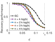
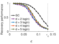
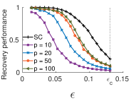
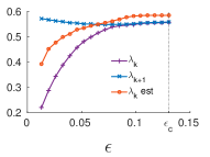
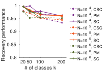
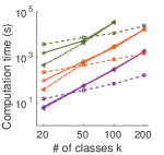
a) b) c) d)
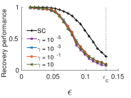
e) f) g) h)

Figure 1: (a-d): recovery performance of CSC on a SBM with $N=10^{3},k=20,s=16$ versus $\epsilon$, for different $n$, $d$, $p$, $\gamma$. Default is $n=2k\log{k}$, $d=4\log{n}$, $p=50$ and $\gamma=10^{-3}$. All results are averaged over 20 graph realisations. e) Estimation of $\lambda_{k}$ (‘$\lambda_{k}$ est’) and the true values of $\lambda_{k}$ and $\lambda_{k+1}$, versus $\epsilon$ on the same SBM. f-g) Performance and time of computation on a SBM with $\epsilon=\epsilon_{c}/4$ and different values of $N$ and $k$; for CSC, PM (Power Method) and SC. For $N=10^{6}$ and $k=200$, we stopped SC (and PM) after 20h of computation. Figures f and g are averaged over 3 graph realisations. N.B.: Fig. f is zoomed around high values of the recovery score, and Fig. g is plotted in log-log. h) Time of computation (in hours) and modularity (in bold) of the obtained partitions for SC and CSC on the Amazon graph. For $k=1000$, SC’s eigendecomposition converges in 17h, and we stopped k-means after 21 hours of computation.

We first perform well-controlled experiments on the Stochastic Block Model (SBM), a model of random graphs with community structure, that was showed suitable as a benchmark for SC in (Lei & Rinaldo, 2015). We also show performance results on a large real-world network. Implementation was done in Matlab R2015a, using the built-in function kmeans with 20 replicates, and the function eigs for SC. Experiments were done on a laptop with a 2.60 GHz Intel i7 dual-core processor running OS Fedora release 22 with 16 GB of RAM. The fast filtering part of CSC uses the gsp$\_$cheby$\_$op function of the GSP toolbox (Perraudin et al., 2014). Equation (7) is solved using Matlab’s gmres function. All our results are reproducible with the CSCbox downloadable at http://cscbox.gforge.inria.fr/.

5.1 The Stochastic Block Model

What distinguishes the SBM from Erdos-Renyi graphs is that the probability of connection between two nodes $i$ and $j$ is not uniform, but depends on the community label of $i$ and $j$. More precisely, the probability of connection between nodes $i$ and $j$ equals $q_{1}$ if they are in the same community, and $q_{2}$ if not. In a first approach, we look at graphs with $k$ communities, all of same size $N/k$. Furthermore, instead of considering the probabilities, one may fully characterize a SBM by providing their ratio $\epsilon=\frac{q_{2}}{q_{1}}$, as well as the average degree $s$ of the graph. The larger $\epsilon$, the more difficult the community structure’s detection. In fact, Decelle et al. (2011) show that a critical value $\epsilon_{c}$ exists above which community detection is impossible at the large $N$ limit: $\epsilon_{c}=(s-\sqrt{s})/(s+\sqrt{s}(k-1))$.

5.2 Performance results

In Figs. 2 a-d), we compare the recovery performance of CSC versus SC for different parameters. The performance is measured by the Adjusted Rand similarity index (Hubert & Arabie, 1985) between the SBM’s ground truth and the obtained partitions. It varies between $-1$ and $1$. The higher it is, the better is the reconstruction. These figures show that the performance of CSC saturates at the default values of $n,d,p$ and $\gamma$ (see top of Alg. 2). Experiments on the SBM with heterogeneous community sizes are provided in the supplementary material and show similar results.

Fig. 2 e) shows the estimation results of $\lambda_{k}$ for different values of $\epsilon$ : it is overestimated in the SBM context. As long as the estimated value stays under $\lambda_{k+1}$, this overestimation does not have a strong impact on the method. On the other hand, as $\epsilon$ becomes larger than $\sim 0.06$, our estimation of $\lambda_{k}$ is larger than $\lambda_{k+1}$, which means that our feature vectors start to integrate some unwanted information from eigenvectors outside of ${\rm span}{(\mathsf{U}_{k})}$. Even though the impact of this additional information is application-dependent and in some cases insignificant, further efforts to improve the estimation of $\lambda_{k}$ would be beneficial to our method.

In Figs. 2 f-g) we fix $\epsilon$ to $\epsilon_{c}/4$, $n,d,p$ and $\gamma$ to the values given in Alg. 2, and vary $N$ and $k$. We compare the recovery performance and the time of computation of CSC, SC and Boutsidis’ power method (Boutsidis & Gittens, 2015). The power method (PM), in a nutshell, 1) applies the Laplacian matrix to the power $r$ to $k$ random signals, 2) computes the left singular vectors of the $N\times k$ obtained matrix, to extract feature vectors, 3) applies $k$-means in high-dimension (like SC) with these feature vectors. In our experiments, we use $r=10$. The recovery performances are nearly identical in all situations, even though CSC is only a few percents under SC and PM (Fig. f is zoomed around the high values of the recovery score). For the time of computation, the experiments confirm that all three methods are roughly linear in $N$ and polynomial in $k$ (Fig. g is plotted in log-log), with a lower exponent for CSC than for SC and PM; such that SC and PM are faster for $k=20$ but CSC becomes up to an order of magnitude faster as $k$ increases to 200. Note that the SBM is favorable to SC as Matlab’s function eigs converges very fast in this case, e.g., for $N=10^{5}$, it finds the first $k=200$ eigenvectors in less than 2 minutes! PM sidesteps successfully the cost of eigs, but the cost of $k$-means in high-dimension is still a strong bottleneck.

We finally compare CSC and SC on a real-world dataset: the Amazon co-purchasing network (Yang & Leskovec, 2015). It is an undirected connected graph comprising $N=334\,863$ nodes and $\#\mathcal{E}=925\,872$ edges. The results are presented in Fig.2 h) for three values of $k$. As there is no clear ground truth in this case, we use the modularity (Newman & Girvan, 2004) to measure the algorithm’s clustering performance, a well-known cost function that measures how well a given partition separates a network in different communities. Note that the 20 replicates of $k$-means would not converge for SC with the default maximum number of iterations set to $100$. For a fair comparison with CSC, we used only 2 replicates with a maximum number of iterations set to $1000$ for SC’s $k$-means step. We see that for the same clustering performance, CSC is much faster than SC, especially as $k$ increases. The PM algorithm on this dataset does not perform well: even though the features are estimated quickly, they apparently do not form clear classes such that its $k$-means step takes even longer than SC’s. For the three values of $k$, we stopped the PM algorithm after a time of computation exceeding SC’s.

6 Conclusion

By graph filtering $O(\log k)$ random signals, we construct feature vectors whose interdistances approach the standard SC feature distances. Then, building upon compressive sensing results, we show that one can sample $O(k\log k)$ nodes from the set of $N$ nodes, cluster this reduced set of nodes and interpolate the result back to the whole graph. If the low-dimensional $k$-means result is correct, i.e., if Eq. (3) is verified, we guarantee that the interpolation is a good approximation of the SC result. To improve the clustering result of the reduced set of nodes, one could consider the concept of community cores (Seifi et al., 2013). In fact, as the filtering and the low-dimensional clustering steps are fairly cheap to compute, one could repeat these steps for different random signals, keep the sets of nodes that are always classified together and use only these stable “cores” for interpolation. Our experiments show that even without such potential improvements, CSC proves efficient and accurate in synthetic and real-world datasets; and could be preferred to SC for large $N$ and/or $k$.

7 Acknowledgments

This article was submitted when G. Puy was with INRIA Rennes - Bretagne Atlantique, France. This work was partly funded by the European Research Council, PLEASE project (ERC-StG-2011-277906), and by the Swiss National Science Foundation, grant 200021-154350/1 - Towards Signal Processing on Graphs.

Appendix A Proof of Theorem 3.2

Proof.

Note that $\mathsf{H}_{\lambda_{k}}=\mathsf{U}_{k}\mathsf{U}_{k}^{\intercal}$, and that $\mathsf{Y}_{k}=\mathsf{V}_{k}\mathsf{U}_{k}$. We rewrite $\left\|\tilde{\bm{f}}_{i}-\tilde{\bm{f}}_{j}\right\|$ in a form that will let us apply the Johnson-Lindenstrauss lemma of norm conservation:

$$\left\|\tilde{\bm{f}}_{i}-\tilde{\bm{f}}_{j}\right\| =\left\|\mathsf{R}^{\intercal}\mathsf{H}_{\lambda_{k}}^{\intercal}\mathsf{V}_{k}^{\intercal}(\bm{\delta}_{i}-\bm{\delta}_{j})\right\|$$ (12)

$$=\left\|\mathsf{R}^{\intercal}\mathsf{U}_{k}\mathsf{U}_{k}^{\intercal}\mathsf{V}_{k}^{\intercal}(\bm{\delta}_{i}-\bm{\delta}_{j})\right\|$$

$$=\left\|\mathsf{R}^{\intercal}\mathsf{U}_{k}(\bm{f}_{i}-\bm{f}_{j})\right\|$$

where the $\bm{f}_{i}$ are the standard SC feature vectors. Applying Theorem 1.1 of (Achlioptas, 2003) (an instance of the Johnson-Lindenstrauss lemma) to $\left\|\mathsf{R}^{\intercal}\mathsf{U}_{k}(\bm{f}_{i}-\bm{f}_{j})\right\|$, the following holds. If $d$ is larger than:

$$\frac{4+2\beta}{\epsilon^{2}/2-\epsilon^{3}/3}\log{N},$$ (13)

then with probability at least $1-N^{-\beta}$, we have, $\forall(i,j)\in\{1,\ldots,N\}^{2}$:

$$(1-\epsilon)\left\|\mathsf{U}_{k}(\bm{f}_{i}-\bm{f}_{j})\right\|\leqslant\tilde{D}_{ij}\leqslant(1+\epsilon)\left\|\mathsf{U}_{k}(\bm{f}_{i}-\bm{f}_{j})\right\|.$$

As the columns of $\mathsf{U}_{k}$ are orthonormal, we end the proof:

$$\forall(i,j)\in[1,N]^{2}\quad\left\|\mathsf{U}_{k}(\bm{f}_{i}-\bm{f}_{j})\right\|=\left\|\bm{f}_{i}-\bm{f}_{j}\right\|=D_{ij}.$$

∎

Appendix B Proof of Theorem 4.1

Proof.

Recall that: $\tilde{D}_{ij}^{r}:=\left\|\tilde{\bm{f}}_{\omega_{i}}-\tilde{\bm{f}}_{\omega_{j}}\right\|=\left\|\mathsf{R}^{\intercal}\mathsf{\tilde{H}}_{\lambda_{k}}^{\intercal}\mathsf{V}_{k}^{\intercal}\mathsf{M}^{\intercal}\bm{\delta}_{ij}^{r}\right\|,$ where $\bm{\delta}_{ij}^{r}=\bm{\delta}_{i}^{r}-\bm{\delta}_{j}^{r}$. Given that $\mathsf{\tilde{H}}_{\lambda_{k}}=\mathsf{H}_{\lambda_{k}}+\mathsf{E}$ and using the triangle inequality in the definition of $\tilde{D}_{ij}^{r}$, we obtain

$$\left\|\mathsf{R}^{\intercal}\mathsf{H}_{\lambda_{k}}^{\intercal}\mathsf{V}_{k}^{\intercal}\mathsf{M}^{\intercal}\bm{\delta}_{ij}^{r}\right\|\;-$$

$$\hskip 8.53581pt\left\|\mathsf{R}^{\intercal}\mathsf{E}^{\intercal}\mathsf{V}_{k}^{\intercal}\mathsf{M}^{\intercal}\bm{\delta}_{ij}^{r}\right\|\leqslant\tilde{D}_{ij}^{r}\leqslant\left\|\mathsf{R}^{\intercal}\mathsf{E}^{\intercal}\mathsf{V}_{k}^{\intercal}\mathsf{M}^{\intercal}\bm{\delta}_{ij}^{r}\right\|\;+$$ (14)

$$\hskip 128.0374pt\left\|\mathsf{R}^{\intercal}\mathsf{H}_{\lambda_{k}}^{\intercal}\mathsf{V}_{k}^{\intercal}\mathsf{M}^{\intercal}\bm{\delta}_{ij}^{r}\right\|,$$

We continue the proof by bounding $\left\|\mathsf{R}^{\intercal}\mathsf{H}_{\lambda_{k}}^{\intercal}\mathsf{V}_{k}^{\intercal}\mathsf{M}^{\intercal}\,\bm{\delta}_{ij}^{r}\right\|$ and $\left\|\mathsf{R}^{\intercal}\mathsf{E}^{\intercal}\mathsf{V}_{k}^{\intercal}\mathsf{M}^{\intercal}\,\bm{\delta}_{ij}^{r}\right\|$ separately.

Let $\delta\in]0,1]$. To bound $\left\|\mathsf{R}^{\intercal}\mathsf{H}_{\lambda_{k}}^{\intercal}\mathsf{V}_{k}^{\intercal}\mathsf{M}^{\intercal}\bm{\delta}_{ij}^{r}\right\|$, we set $\epsilon=\delta/2$ in Theorem 3.2. This proves that if $d$ is larger than

$$d_{0}=\frac{16(2+\beta)}{\delta^{2}-\delta^{3}/3}\log{n},$$

then with probability at least $1-n^{-\beta}$,

$$\left(1-\frac{\delta}{2}\right)D_{ij}^{r}\leqslant\left\|\mathsf{R}^{\intercal}\mathsf{H}_{\lambda_{k}}^{\intercal}\mathsf{V}_{k}^{\intercal}\mathsf{M}^{\intercal}\bm{\delta}_{ij}^{r}\right\|\leqslant\left(1+\frac{\delta}{2}\right)D_{ij}^{r},$$

for all $(i,j)\in\{1,\ldots,n\}^{2}$. To bound $\left\|\mathsf{R}^{\intercal}\mathsf{E}^{\intercal}\mathsf{V}_{k}^{\intercal}\mathsf{M}^{\intercal}\bm{\delta}_{ij}^{r}\right\|$, we use Theorem $1.1$ in (Achlioptas, 2003). This theorem proves that if $d>d_{0}$, then with probability at least $1-n^{-\beta}$,

$$\left\|\mathsf{R}^{\intercal}\mathsf{E}^{\intercal}\mathsf{V}_{k}^{\intercal}\mathsf{M}^{\intercal}\bm{\delta}_{ij}^{r}\right\|\leqslant\left(1+\frac{\delta}{2}\right)\left\|\mathsf{E}^{\intercal}\mathsf{V}_{k}^{\intercal}\mathsf{M}^{\intercal}\bm{\delta}_{ij}^{r}\right\|,$$

for all $(i,j)\in\{1,\ldots,n\}^{2}$. Using the union bound and (B), we deduce that, with probability at least $1-2n^{-\beta}$,

$$\left(1-\frac{\delta}{2}\right)D_{ij}^{r}-\left(1+\frac{\delta}{2}\right)\left\|\mathsf{E}^{\intercal}\mathsf{V}_{k}^{\intercal}\mathsf{M}^{\intercal}\bm{\delta}_{ij}^{r}\right\|$$

$$\hskip 71.13188pt\leqslant\quad\tilde{D}_{ij}^{r}\quad\leqslant$$ (15)

$$\hskip 28.45274pt\left(1+\frac{\delta}{2}\right)\left\|\mathsf{E}^{\intercal}\mathsf{V}_{k}^{\intercal}\mathsf{M}^{\intercal}\bm{\delta}_{ij}^{r}\right\|\;+\left(1+\frac{\delta}{2}\right)D_{ij}^{r},$$

for all $(i,j)\in\{1,\ldots,n\}^{2}$ provided that $d>d_{0}$.

Then, as $e$ is bounded by $e_{1}$ on the first $k$ eigenvalues of the spectrum and by $e_{2}$ on the remaining ones, we have

$$\left\|\mathsf{E}^{\intercal}\mathsf{V}_{k}^{\intercal}\mathsf{M}^{\intercal}\,\bm{\delta}_{ij}^{r}\right\|^{2} =\left\|\mathsf{U}e(\mathsf{\Lambda})\mathsf{U}^{\intercal}\mathsf{V}_{k}^{\intercal}\mathsf{M}^{\intercal}\,\bm{\delta}_{ij}^{r}\right\|^{2}$$

$$=\left\|e(\mathsf{\Lambda})\mathsf{U}^{\intercal}\mathsf{V}_{k}^{\intercal}\mathsf{M}^{\intercal}\,\bm{\delta}_{ij}^{r}\right\|^{2}$$

$$=\;\sum_{l=1}^{N}e(\lambda_{l})^{2}\,\left|(\mathsf{M}\mathsf{V}_{k}\bm{u}_{l})^{\intercal}\bm{\delta}_{ij}^{r}\right|^{2}$$

$$\;\leqslant\;e_{1}^{2}\;\sum_{l=1}^{k}\left|(\mathsf{M}\mathsf{V}_{k}\bm{u}_{l})^{\intercal}\bm{\delta}_{ij}^{r}\right|^{2}$$

$$\hskip 28.45274pt+e_{2}^{2}\;\sum_{l=k+1}^{N}\left|(\mathsf{M}\mathsf{V}_{k}\bm{u}_{l})^{\intercal}\bm{\delta}_{ij}^{r}\right|^{2}$$

$$=e_{1}^{2}\;\left\|\mathsf{U}_{k}^{\intercal}\mathsf{V}_{k}^{\intercal}\mathsf{M}^{\intercal}\bm{\delta}_{ij}^{r}\right\|^{2}$$

$$+e_{2}^{2}\;\left(\left\|\mathsf{U}^{\intercal}\mathsf{V}_{k}^{\intercal}\mathsf{M}^{\intercal}\bm{\delta}_{ij}^{r}\right\|^{2}-\left\|\mathsf{U}_{k}^{\intercal}\mathsf{V}_{k}^{\intercal}\mathsf{M}^{\intercal}\bm{\delta}_{ij}^{r}\right\|^{2}\right)$$

$$=\;(e_{1}^{2}-e_{2}^{2})\;\left\|\mathsf{U}_{k}^{\intercal}\mathsf{V}_{k}^{\intercal}\mathsf{M}^{\intercal}\bm{\delta}_{ij}^{r}\right\|^{2}$$

$$\hskip 28.45274pt+e_{2}^{2}\;\left\|\mathsf{U}^{\intercal}\mathsf{V}_{k}^{\intercal}\mathsf{M}^{\intercal}\bm{\delta}_{ij}^{r}\right\|^{2}$$

$$=(e_{1}^{2}-e_{2}^{2})\;(D_{ij}^{r})^{2}+e_{2}^{2}\;\left\|\mathsf{V}_{k}^{\intercal}\mathsf{M}^{\intercal}\bm{\delta}_{ij}^{r}\right\|^{2}$$

$$\leqslant(e_{1}^{2}-e_{2}^{2})\,(D_{ij}^{r})^{2}+\frac{2\,e_{2}^{2}}{\min_{i}\{v_{k}(i)^{2}\}}.$$

The last step follows from the fact that

$$\left\|\mathsf{V}_{k}^{\intercal}\mathsf{M}^{\intercal}\,\bm{\delta}_{ij}^{r}\right\|^{2} =\sum_{l=1}^{N}\frac{1}{v_{k}(l)^{2}}\left|(\mathsf{M}^{\intercal}\bm{\delta}_{ij}^{r})(l)\right|^{2}$$

$$=\frac{1}{v_{k}(\omega_{i})^{2}}+\frac{1}{v_{k}(\omega_{j})^{2}}\,\leqslant\,\frac{2}{\min_{i}\{v_{k}(i)\}^{2}}$$

Define, for all $(i,j)\in\{1,\ldots,n\}^{2}$:

$$e_{ij}:=\sqrt{\left|e_{1}^{2}-e_{2}^{2}\right|}D_{ij}^{r}+\frac{\sqrt{2}e_{2}}{\min_{i}\{v_{k}(i)\}}.$$

Thus, the above inequality may be rewritten as:

$$\left\|\mathsf{E}^{\intercal}\mathsf{V}_{k}^{\intercal}\mathsf{M}^{\intercal}\,\bm{\delta}_{ij}^{r}\right\|\leqslant e_{ij},$$

for all $(i,j)\in\{1,\ldots,n\}^{2}$, which combined with (B) yields

$$\left(1-\frac{\delta}{2}\right)D_{ij}^{r}-\left(1+\frac{\delta}{2}\right)e_{ij}$$

$$\hskip 85.35826pt\leqslant\quad\tilde{D}_{ij}^{r}\quad\leqslant$$ (16)

$$\hskip 99.58464pt\left(1+\frac{\delta}{2}\right)e_{ij}\;+\left(1+\frac{\delta}{2}\right)D_{ij}^{r},$$

for all $(i,j)\in\{1,\ldots,n\}^{2}$, with probability at least $1-2n^{-\beta}$ provided that $d>d_{0}$.

Let us now separate two cases. In the case where $D_{ij}^{r}\geqslant D_{min}^{r}>0$, we have

$$e_{ij} =\frac{e_{ij}}{D_{ij}^{r}}D_{ij}^{r}=\left(\sqrt{|e_{1}^{2}-e_{2}^{2}|}+\frac{\sqrt{2}e_{2}}{D_{ij}^{r}\,\min_{i}\{v_{k}(i)\}}\right)D_{ij}^{r}$$

$$\leqslant\left(\sqrt{|e_{1}^{2}-e_{2}^{2}|}+\frac{\sqrt{2}e_{2}}{D_{min}^{r}\,\min_{i}\{v_{k}(i)\}}\right)D_{ij}^{r}$$

$$\leqslant\frac{\delta}{2+\delta}D_{ij}^{r}.$$

provided that Eq. (7) of the main paper holds. Combining the last inequality with (B) proves the first part of the theorem.

In the case where $D_{ij}^{r}<D_{min}^{r}$, we have

$$e_{ij}<\sqrt{|e_{1}^{2}-e_{2}^{2}|}D_{min}^{r}+\frac{\sqrt{2}\,e_{2}}{\min_{i}\{v_{k}(i)\}}\leqslant\frac{\delta}{2+\delta}D_{min}^{r}.$$

provided that Eq. (7) of the main paper holds. Combining the last inequality with (B) terminates the proof. ∎

Appendix C Experiments on the SBM with heterogeneous community sizes

We perform experiments on a SBM with $N=10^{3},k=20,s=16$ and hetereogeneous community sizes. More specifically, the list of community sizes is chosen to be: $5$, $10$, $15$, $20$, $25$, $30$, $35$, $40$, $45$, $50$, $50$, $55$, $60$, $65$, $70$, $75$, $80$, $85$, $90$ and $95$ nodes. In this scenario, there is no theoretical value of $\epsilon$ over which it is proven that recovery is impossible in the large $N$ limit. Instead, we vary $\epsilon$ between $0$ and $0.2$ and show the recovery performance results with respect to $n$, $d$, $p$ and $\gamma$ in Fig. 2. Results are similar to the homogeneous case presented in Fig. 1(a-d) of the main paper.

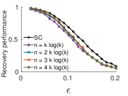
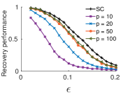
a) b)
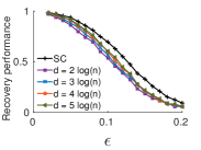
c) d)

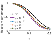
Figure 2: (a-d): recovery performance of CSC on a SBM with $N=10^{3},k=20,s=16$ and hetereogeneous community sizes versus $\epsilon$, for different $n$, $d$, $p$, $\gamma$. Default is $n=2k\log{k}$, $d=4\log{n}$, $p=50$ and $\gamma=10^{-3}$. All results are averaged over 20 graph realisations.

References

- Achlioptas (2003) Achlioptas, D. Database-friendly random projections: Johnson-lindenstrauss with binary coins. Journal of Computer and System Sciences, 66(4):671 – 687, 2003.
- Anis et al. (2015) Anis, A., Gadde, A., and Ortega, A. Efficient sampling set selection for bandlimited graph signals using graph spectral proxies. arXiv, abs/1510.00297, 2015.
- Belkin & Niyogi (2003) Belkin, M. and Niyogi, P. Laplacian eigenmaps for dimensionality reduction and data representation. Neural computation, 15(6):1373–1396, 2003.
- Boutsidis et al. (2011) Boutsidis, C., Zouzias, A., Mahoney, M. W, and Drineas, P. Stochastic dimensionality reduction for k-means clustering. arXiv, abs/1110.2897, 2011.
- Boutsidis & Gittens (2015) Boutsidis, C., Kambadur P. and Gittens, A. Spectral clustering via the power method - provably. In Proceedings of the 32nd International Conference on Machine Learning (ICML-15), Lille, France, pp. 40–48, 2015.
- Chen et al. (2015) Chen, S., Varma, R., Sandryhaila, A., and Kovacevic, J. Discrete signal processing on graphs: Sampling theory. Signal Processing, IEEE Transactions on, 63(24):6510–6523, 2015.
- Chen et al. (2011) Chen, W.-Y., Song, Y., Bai, H., C.-J, Lin., and Chang, E.Y. Parallel spectral clustering in distributed systems. Pattern Analysis and Machine Intelligence, IEEE Transactions on, 33(3):568–586, 2011.
- Chen & Cai (2011) Chen, X. and Cai, D. Large scale spectral clustering with landmark-based representation. In Proceedings of the 25th AAAI Conference on Artificial Intelligence, 2011.
- Chung (1997) Chung, F.R.K. Spectral graph theory. Number 92. Amer Mathematical Society, 1997.
- Cohen et al. (2015) Cohen, M. B., Elder, S., Musco, C., Musco, C., and Persu, M. Dimensionality reduction for k-means clustering and low rank approximation. In Proceedings of the 47th Annual ACM on Symposium on Theory of Computing, pp. 163–172. ACM, 2015.
- Decelle et al. (2011) Decelle, A., Krzakala, F., Moore, C, and Zdeborová, L. Asymptotic analysis of the stochastic block model for modular networks and its algorithmic applications. Phys. Rev. E, 84:066106, 2011.
- Dhillon et al. (2007) Dhillon, I.S., Guan, Y., and Kulis, B. Weighted graph cuts without eigenvectors a multilevel approach. Pattern Analysis and Machine Intelligence, IEEE Transactions on, 29(11):1944–1957, 2007.
- Fiedler (1973) Fiedler, M. Algebraic connectivity of graphs. Czechoslovak mathematical journal, 23(2):298–305, 1973.
- Filippone et al. (2008) Filippone, M., Camastra, F., Masulli, F., and Rovetta, S. A survey of kernel and spectral methods for clustering. Pattern Recognition, 41(1):176 – 190, 2008.
- Fowlkes et al. (2004) Fowlkes, C., Belongie, S., Chung, F., and Malik, J. Spectral grouping using the nystrom method. Pattern Analysis and Machine Intelligence, IEEE Transactions on, 26(2):214–225, 2004.
- Har-Peled & Mazumdar (2004) Har-Peled, Sariel and Mazumdar, Soham. On coresets for k-means and k-median clustering. In Proceedings of the thirty-sixth annual ACM symposium on Theory of computing, pp. 291–300. ACM, 2004.
- Hubert & Arabie (1985) Hubert, L. and Arabie, P. Comparing partitions. Journal of classification, 2(1):193–218, 1985.
- Jain (2010) Jain, Anil K. Data clustering: 50 years beyond k-means. Pattern Recognition Letters, 31(8):651 – 666, 2010.
- Lei & Rinaldo (2015) Lei, J. and Rinaldo, A. Consistency of spectral clustering in stochastic block models. Ann. Statist., 43(1):215–237, 2015.
- Lin & Cohen (2010) Lin, F. and Cohen, W. W. Power iteration clustering. In Proceedings of the 27th International Conference on Machine Learning (ICML-10), Haifa, Israel, pp. 655–662, 2010.
- Liu et al. (2007) Liu, T.-Y., Yang, H.-Y., Zheng, X., Qin, T., and Ma, W.-Y. Fast large-scale spectral clustering by sequential shrinkage optimization. In Advances in Information Retrieval, pp. 319–330. 2007.
- Marques et al. (2015) Marques, A., Segarra, S., Leus, G., and Ribeiro, A. Sampling of graph signals with successive local aggregations. Signal Processing, IEEE Transactions on, PP(99):1–1, 2015.
- Napoli et al. (2013) Napoli, Edoardo Di, Polizzi, Eric, and Saad, Yousef. Efficient estimation of eigenvalue counts in an interval. arXiv, abs/1308.4275, 2013.
- Nascimento & de Carvalho (2011) Nascimento, M.C.V. and de Carvalho, A.C.P.L.F. Spectral methods for graph clustering – a survey. European Journal of Operational Research, 211(2):221 – 231, 2011.
- Newman & Girvan (2004) Newman, M. E. J. and Girvan, M. Finding and evaluating community structure in networks. Phys. Rev. E, 69:026113, 2004.
- Ng et al. (2002) Ng, A.Y., Jordan, M.I., and Weiss, Y. On spectral clustering: Analysis and an algorithm. In Dietterich, T.G., Becker, S., and Ghahramani, Z. (eds.), Advances in Neural Information Processing Systems 14, pp. 849–856. MIT Press, 2002.
- Perraudin et al. (2014) Perraudin, N., Paratte, J., Shuman, D., Kalofolias, V., Vandergheynst, P., and Hammond, D.K. Gspbox: A toolbox for signal processing on graphs. arXiv, abs/1408.5781, 2014.
- Puy et al. (2015) Puy, G., Tremblay, N., Gribonval, R., and Vandergheynst, P. Random sampling of bandlimited signals on graphs. arXiv, abs/1511.05118, 2015.
- Ramasamy & Madhow (2015) Ramasamy, D. and Madhow, U. Compressive spectral embedding: sidestepping the SVD. In Advances in Neural Information Processing Systems 28, pp. 550–558. 2015.
- Sakai & Imiya (2009) Sakai, Tomoya and Imiya, Atsushi. Fast spectral clustering with random projection and sampling. In Machine Learning and Data Mining in Pattern Recognition, pp. 372–384. 2009.
- Sandryhaila & Moura (2013) Sandryhaila, A. and Moura, J.M.F. Discrete signal processing on graphs. Signal Processing, IEEE Transactions on, 61(7):1644–1656, 2013.
- Sandryhaila & Moura (2014) Sandryhaila, A. and Moura, J.M.F. Big data analysis with signal processing on graphs: Representation and processing of massive data sets with irregular structure. Signal Processing Magazine, IEEE, 31(5):80–90, 2014.
- Seifi et al. (2013) Seifi, M., Junier, I., Rouquier, J.-B., Iskrov, S., and Guillaume, J.-L. Stable community cores in complex networks. In Complex Networks, pp. 87–98. 2013.
- Shi & Malik (2000) Shi, J. and Malik, J. Normalized cuts and image segmentation. Pattern Analysis and Machine Intelligence, IEEE Transactions on, 22(8):888–905, 2000.
- Shi et al. (2015) Shi, X., Feng, H., Zhai, M., Yang, T., and Hu, B. Infinite impulse response graph filters in wireless sensor networks. Signal Processing Letters, IEEE, 22(8):1113–1117, 2015.
- Shuman et al. (2011) Shuman, D.I., Vandergheynst, P., and Frossard, P. Chebyshev polynomial approximation for distributed signal processing. In Distributed Computing in Sensor Systems and Workshops (DCOSS), International Conference on, pp. 1–8, 2011.
- Shuman et al. (2013) Shuman, D.I., Narang, S.K., Frossard, P., Ortega, A., and Vandergheynst, P. The emerging field of signal processing on graphs: Extending high-dimensional data analysis to networks and other irregular domains. Signal Processing Magazine, IEEE, 30(3):83–98, 2013.
- Tremblay et al. (2016) Tremblay, N., Puy, G., Borgnat, P., Gribonval, R., and Vandergheynst, P. Accelerated spectral clustering using graph filtering of random signals. In Acoustics, Speech and Signal Processing (ICASSP), IEEE International Conference on, 2016. accepted.
- Tsitsvero et al. (2015) Tsitsvero, M., Barbarossa, S., and Lorenzo, P. Di. Signals on graphs: Uncertainty principle and sampling. arXiv, abs/1507.08822, 2015.
- von Luxburg (2007) von Luxburg, U. A tutorial on spectral clustering. Statistics and Computing, 17(4):395–416, 2007.
- Wang et al. (2009) Wang, L., Leckie, C., Ramamohanarao, K., and Bezdek, J. Approximate spectral clustering. In Advances in Knowledge Discovery and Data Mining, pp. 134–146. 2009.
- White & Smyth (2005) White, S. and Smyth, P. A spectral clustering approach to finding communities in graph. In SDM, volume 5, pp. 76–84. SIAM, 2005.
- Yan et al. (2009) Yan, D., Huang, L., and Jordan, M.I. Fast approximate spectral clustering. In Proceedings of the 15th ACM SIGKDD International Conference on Knowledge Discovery and Data Mining, KDD ’09, pp. 907–916, New York, NY, USA, 2009.
- Yang & Leskovec (2015) Yang, J. and Leskovec, J. Defining and evaluating network communities based on ground-truth. Knowledge and Information Systems, 42(1):181–213, 2015.
- Zelnik-Manor & Perona (2004) Zelnik-Manor, L. and Perona, P. Self-tuning spectral clustering. In Advances in neural information processing systems, pp. 1601–1608, 2004.