Imaginary projections of polynomials

Abstract.

We introduce the imaginary projection of a multivariate polynomial $f\in\mathbb{C}[\mathbf{z}]$ as the projection of the variety of $f$ onto its imaginary part, $\mathcal{I}(f)\ =\ \{\operatorname{Im}(\mathbf{z})\,:\,\mathbf{z}\in\mathcal{V}(f)\}$. Since a polynomial $f$ is stable if and only if $\mathcal{I}(f)\cap\mathbb{R}_{>0}^{n}\ =\ \emptyset$, the notion offers a novel geometric view underlying stability questions of polynomials.

We show that the connected components of the complement of the closure of the imaginary projections are convex, thus opening a central connection to the theory of amoebas and coamoebas. Building upon this, the paper establishes structural properties of the components of the complement, such as lower bounds on their maximal number, proves a complete classification of the imaginary projections of quadratic polynomials and characterizes the limit directions for polynomials of arbitrary degree.

1. Introduction

Recent years have seen a lot of interest in stable polynomials, see, e.g., [5, 6, 20, 30] and the references therein. A polynomial $f=f(\mathbf{z})=f(z_{1},\ldots,z_{n})\in\mathbb{C}[\mathbf{z}]=\mathbb{C}[z_{1},\ldots,z_{n}]$ is called stable if every root $\mathbf{z}$ satisfies $\operatorname{Im}(z_{j})\leq 0$ for some $j$. We call $f$ real stable if $f$ has real coefficients and is stable.

As recent prominent applications, Marcus, Spielman, and Srivastava employed stable polynomials in the proof of the Kadison-Singer Conjecture [20] and in the existence proof of families of bipartite Ramanujan graphs of every degree larger than two [19]. Stable polynomials have also been used by Borcea and Brändén to prove Johnson’s Conjecture [5] and in Gurvits’ simple proof of a generalization of van der Waerden’s Conjecture for permanents [15]. Moreover, there are strong connections to hyperbolic polynomials and their hyperbolicity cones, see Section 2.1.

In this paper, we initiate to study the underlying projections on the imaginary parts from a geometric point of view. Given a polynomial $f\in\mathbb{C}[\mathbf{z}]$, introduce the imaginary projection of $f$ as

$$\mathcal{I}(f)\ =\ \left\{\operatorname{Im}(\mathbf{z})\,:\,\mathbf{z}\in\mathcal{V}(f)\right\}\ \subseteq\ \mathbb{R}^{n}\,,$$

where $\mathcal{V}(f)$ denotes the variety of $f$ and $\operatorname{Im}(\mathbf{z})=(\operatorname{Im}(z_{1}),\ldots,\operatorname{Im}(z_{n}))$. So, in particular, $f$ is stable if and only if

$$\mathcal{I}(f)\cap\mathbb{R}_{>0}^{n}\ =\ \emptyset\,.$$

Our work is motivated by the theory of amoebas as well as by the general goal to reveal and understand convexity phenomena in algebraic geometry, see [3]. Amoebas are the images of algebraic varieties in the algebraic torus $(\mathbb{C}^{*})^{n}$ under the log-absolute map:

$$\mathcal{A}(f)\ =\ \{(\log|z_{1}|,\ldots,\log|z_{n}|)\,:\,\mathbf{z}\in\mathcal{V}(f)\cap(\mathbb{C}^{*})^{n}\}\ \subseteq\ \mathbb{R}^{n}\,,$$

see [13]. Coamoebas employ the arg-map rather than the log-absolute map; see, e.g., [11].

For amoebas, important structural results as well as their occurrences in a broad spectrum of mathematical disciplines have been intensively studied, see [21, 23, 24] as well as the recent survey [31]. For coamoebas, investigations are much more recent [11, 12, 22]. A prominent result states that the complement of an amoeba as well as the complement of the closure of a coamoeba consists of finitely many convex components, see [12, 13]. As a key result, which also motivates our study, we show that the closure of the complement of the imaginary projection of a polynomial consists of finitely many convex components as well, see Theorem 4.1.

While there are important analogies among amoebas, coamoebas, and imaginary projections, there are also fundamental differences between these structures. The fibers of the log-absolute maps underlying amoebas are compact, whereas for imaginary projections they are not compact. Furthermore, the limit directions of amoebas, also known as tentacles, are characterized by the logarithmic limit sets and thus carry a polyhedral structure; see [18, Theorem 1.4.2]. In contrast, the limit directions of the imaginary projections are not polyhedral in general, see Section 6. For coamoebas, which are defined on a torus, Nisse and Sottile have introduced a variant of the logarithmic limit sets, by considering accumulation points of arguments of sequences with unbounded logarithm [22].

Building upon the fundamental convexity result, we study structural properties of imaginary projections. We also give lower bounds on the maximal number of components of the complement, see Corollary 4.5.

We investigate important subclasses, such as quadratic and multilinear polynomials. For the class of real quadratic polynomials, we can provide a complete classification of the imaginary projections, see Theorem 5.4. Indeed, this classification result in Theorem 5.4 is somewhat unexpected, since it involves various qualitatively different cases.

Starting from the well-known results on tentacles of amoebas, we characterize the limit points of the imaginary projections. Contrary to the case of the amoeba of a non-zero polynomial $f$, it is possible that every point on the sphere $\mathbb{S}^{n-1}$ is a limit direction of the imaginary projection of $f$. For $f\in\mathbb{C}[\mathbf{z}]$, we provide a criterion for one-dimensional families of limit directions at infinity. In the case $n=2$ this also characterizes the situations that all points are limit points. See Theorem 6.5 and Corollary 6.7 for further details.

It is easy to see that real projections of complex polynomials should behave in the same way as imaginary projections, since one projection is easily seen to be an instance of the other by replacing the polynomial $f(x)$ with $f(\sqrt{-1}x)$. However, we focus on imaginary projections since the latter projections are more naturally connected to stability and hyperbolicity in the setting of real polynomials.

Our paper is structured as follows. Section 2 collects existing facts on stable polynomials as well as on amoebas and coamoebas. In Section 3, we study the structure of imaginary projections. Section 4 considers the components of the complement. In Section 5, we discuss quadratic and multilinear (in the sense of multi-affine-linear) polynomials, and Section 6 is concerned with the situation at infinity. In Section 7 we close with some open questions.

2. Preliminaries

We collect basic notions on stable polynomials as well as on amoebas and coamoebas. Let $\mathbb{R}_{\geq 0}$ and $\mathbb{R}_{>0}$ denote the set of non-negative and the set of strictly positive real numbers.

Throughout the paper, we use bold letters for vectors, e.g., $\mathbf{z}=(z_{1},\ldots,z_{n})\in\mathbb{C}^{n}$. Unless stated otherwise, the dimension of these vectors is $n$. Denote by $\mathcal{V}(f)$ the complex variety of a polynomial $f\in\mathbb{C}[\mathbf{z}]$ and by $\mathcal{V}_{\mathbb{R}}(f)$ the real variety of $f$.

We denote by $\operatorname{Re}(z)$ and $\operatorname{Im}(z)$ the real and the imaginary part of a point $z\in\mathbb{C}$, i.e., $z=\operatorname{Re}(z)+i\operatorname{Im}(z)$, and component-wise for points $\mathbf{z}\in\mathbb{C}^{n}$. For an arbitrary set $M\subseteq\mathbb{C}^{n}$ we understand $\operatorname{Re}(M)$ and $\operatorname{Im}(M)$ as the real parts and the imaginary parts of all elements in $M$. Moreover, for a polynomial $f\in\mathbb{C}[\mathbf{z}]$ we denote by $\operatorname{Re}(f)$ and $\operatorname{Im}(f)$ the real part and the imaginary part of $f$ after the realification $\mathbf{z}=\mathbf{x}+i\mathbf{y}\in\mathbb{C}^{n}\mapsto(\mathbf{x},\mathbf{y})\in\mathbb{R}^{2n}$, i.e., $f(\mathbf{x},\mathbf{y})=\operatorname{Re}f(\mathbf{x},\mathbf{y})+i\operatorname{Im}f(\mathbf{x},\mathbf{y})$. Note that $\operatorname{Re}(f)$ and $\operatorname{Im}(f)$ are real polynomials in $\mathbb{R}[\mathbf{x},\mathbf{y}]$.

Furthermore, we use the notations $\mathcal{H}_{\mathbb{C}}^{n}$ for the set $\{\mathbf{z}\in\mathbb{C}^{n}:\operatorname{Im}(z_{j})>0,\,1\leq j\leq n\}$ and $\mathcal{H}_{\mathbb{R}}^{n}=\operatorname{Im}\mathcal{H}_{\mathbb{C}}^{n}$, which is the positive orthant.

2.1. Stable polynomials

Based on the notions of stability and real stability defined in the introduction, we collect the following statements and properties. As a general source on stability of polynomials, we refer to [30] and the references therein.

Definition 2.1.

A polynomial $f\in\mathbb{C}[\mathbf{z}]$ is called stable if it has no root $\mathbf{z}$ in $\mathcal{H}_{\mathbb{C}}^{n}$.

Example 2.2.

[5, Proposition 2.4] For positive semidefinite $d\times d$-matrices $A_{1},\ldots,A_{n}$ and a Hermitian $d\times d$-matrix $B$, the polynomial

$$f(\mathbf{z})\ =\ \det(z_{1}A_{1}+\cdots+z_{n}A_{n}+B)$$

is real stable or identically zero.

There is a close connection between stable, homogeneous polynomials and hyperbolic polynomials. A homogeneous polynomial $f\in\mathbb{R}[\mathbf{z}]$ is called hyperbolic in direction $\mathbf{e}\in\mathbb{R}^{n}$, if $f(\mathbf{e})\neq 0$ and for every $\mathbf{x}\in\mathbb{R}^{n}$ the real function $t\mapsto f(\mathbf{x}+t\mathbf{e})$ has only real roots. It is known that a homogeneous polynomial $f\in\mathbb{R}[\mathbf{z}]$ is real stable if and only if $f$ is hyperbolic with respect to every point in the positive orthant, see [14, 30].

Stability of univariate polynomials can be tested as follows. Here, we call two univariate polynomials $f,g\in\mathbb{R}[\mathbf{z}]$ in proper position, $f\ll g$, if the zeros of $f$ and $g$ interlace (i.e., alternate, see [8, 19]), and if their Wronskian $W[f,g]:=f^{\prime}g-fg^{\prime}$ is non-negative on $\mathbb{R}$. Note that if the roots of two polynomials $f$ and $g$ interlace, then $W[f,g]$ is non-negative or non-positive.

Theorem 2.3.

(Hermite-Biehler, see [25, Thm. 6.3.4] or [30]) A non-constant univariate polynomial $f\in\mathbb{C}[z]$ is stable if and only if $\operatorname{Im}f\ll\operatorname{Re}f$.

Borcea and Brändén gave the following multivariate generalization of the Hermite-Biehler Theorem. Here, two multivariate polynomials $f,g\in\mathbb{R}[\mathbf{z}]$ are called in proper position, written $f\ll g$, if the univariate polynomials $f(\mathbf{x}+t\mathbf{e})$, $g(\mathbf{x}+t\mathbf{e})$ are in proper position for all $\mathbf{x}\in\mathbb{R}^{n}$, $\mathbf{e}\in\mathbb{R}_{\geq 0}^{n}\setminus\{0\}$.

Theorem 2.4.

([7, Cor. 2.4], see also [8, Thm. 5.3]) A non-constant polynomial $f\in\mathbb{C}[\mathbf{z}]$ is stable if and only if $\operatorname{Im}f\ll\operatorname{Re}f$.

We call a polynomial $f\in\mathbb{C}[\mathbf{z}]$ multilinear if it has degree at most $1$ with respect to each variable. Brändén characterized stability of multilinear polynomials with real coefficients.

Theorem 2.5.

[8, Theorem 5.6] Let $f\in\mathbb{R}[\mathbf{z}]$ be non-constant and multilinear. Then $f$ is stable if and only if for all $1\leq j,k\leq n$ the function

$$\Delta_{jk}(f)\ =\ \frac{\partial f}{\partial z_{j}}\frac{\partial f}{\partial z_{k}}-\frac{\partial^{2}f}{\partial z_{j}\partial z_{k}}\cdot f$$

is non-negative on $\mathbb{R}^{n}$.

Hence, a non-zero bivariate polynomial $f(z_{1},z_{2})=\alpha z_{1}z_{2}+\beta z_{1}+\gamma z_{2}+\delta$ with $\alpha,\beta,\gamma,\delta\in\mathbb{R}$ is real stable if and only if $\beta\gamma-\alpha\delta\geq 0$.

The non-multilinear case can be reduced to the multilinear case via the polarization $\mathcal{P}(f)$ of a multivariate polynomial $f$, see [8]. Denoting by $d_{j}$ the degree of $f$ in the variable $z_{j}$, $\mathcal{P}(f)$ is the unique polynomial in the variables $z_{jk}$, $1\leq j\leq n$, $1\leq k\leq d_{j}$ with the properties

1. $\mathcal{P}(f)$ is multilinear,

2. $\mathcal{P}(f)$ is symmetric in the variables $z_{j1},\ldots,z_{jd_{j}}$, $1\leq j\leq n$,

3. if we apply the substitutions $z_{jk}=z_{j}$ for all $j,k$, then $\mathcal{P}(f)$ coincides with $f$.

By the Grace-Walsh-Szegö Theorem, $\mathcal{P}(f)$ is stable if and only if $f$ is stable; see, e.g., [8, Cor. 5.9].

By Theorem 2.5, deciding whether a multilinear polynomial $f$ is stable is equivalent to deciding whether $\Delta_{jk}(f)\geq 0$ on $\mathbb{R}^{n}$ for all $j,k$. In [17], sum of squares-relaxations are considered to decide this question.

2.2. Amoebas and coamoebas

The theory of amoebas builds upon algebraic varieties in the complex torus $(\mathbb{C}^{\ast})^{n}=(\mathbb{C}\setminus\{0\})^{n}$. For a Laurent polynomial $f\in\mathbb{C}[z_{1}^{\pm 1},\ldots,z_{n}^{\pm 1}]$, define the semialgebraic amoeba $\mathcal{S}(f)$ (also known as unlog amoeba) by

(2.1) $$\mathcal{S}(f)\ =\ \{|\mathbf{z}|=(|z_{1}|,\ldots,|z_{n}|)\in\mathbb{R}^{n}:\mathbf{z}\in\mathcal{V}(f)\cap(\mathbb{C}^{*})^{n}\},$$

and the amoeba $\mathcal{A}(f)$ by

(2.2) $$\mathcal{A}(f)\ =\ \{\log|\mathbf{z}|=(\log|z_{1}|,\ldots,\log|z_{n}|)\in\mathbb{R}^{n}:\mathbf{z}\in\mathcal{V}(f)\cap(\mathbb{C}^{\ast})^{n}\}\,.$$

Amoebas were first introduced and studied by Gelfand, Kapranov and Zelevinsky in [13]. Similarly, the coamoeba of $f$ is defined as

(2.3) $$co\mathcal{A}(f)\ =\ \{\arg(\mathbf{z})=(\arg(z_{1}),\ldots,\arg(z_{n})):\mathbf{z}\in\mathcal{V}(f)\cap(\mathbb{C}^{\ast})^{n}\}\ \subseteq\ \mathbb{T}^{n}\,,$$

where $\arg$ denotes the argument of a complex number and $\mathbb{T}^{n}=\left(\mathbb{R}/2\pi\mathbb{Z}\right)^{n}$.

If $\log_{\mathbb{C}}$ is the complex logarithm, then we have the relations

$$\mathcal{A}(f)=\operatorname{Re}\circ\log_{\mathbb{C}}\mathcal{V}(f)\quad\text{ and }\quad co\mathcal{A}(f)=\operatorname{Im}\circ\log_{\mathbb{C}}\mathcal{V}(f)\,,$$

where all maps are understood component-wise. See Figure 1 for an example of an amoeba and a coamoeba.

We recall some basic statements about amoebas, see [10, 13, 28]. For a Laurent polynomial $f\in\mathbb{C}[\mathbf{z}]$, the amoeba $\mathcal{A}(f)$ is a closed set. The complement of $\mathcal{A}(f)$ consists of finitely many convex regions, and these regions are in bijective correspondence with the different Laurent series expansions of the rational function $1/f$. The number of components in the complement of an amoeba is bounded from above by the number of lattice points in the Newton polytope of $f$ and bounded from below by the number of vertices of the Newton polytope of $f$.

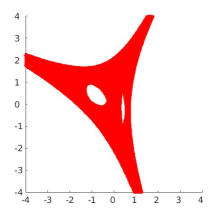
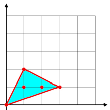
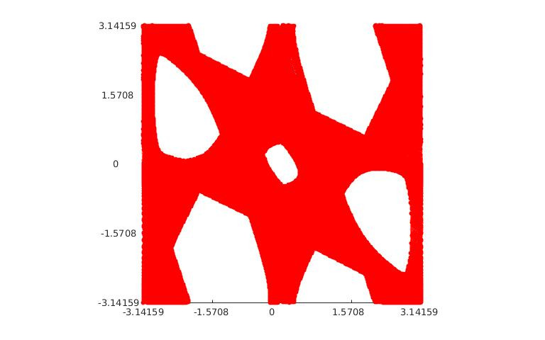
Figure 1. An approximation of the amoeba and the coamoeba of the Laurent polynomial $f(z_{1},z_{2})=2z_{1}^{3}z_{2}+z_{1}z_{2}^{2}-4z_{1}z_{2}-2.5\cdot e^{0.7\cdot\pi\cdot i}z_{1}^{2}z_{2}+1$ together with its corresponding Newton polytope.

For coamoebas, it has been conjectured that the complement of the closure of $co\mathcal{A}(f)$ contains at most $n!\operatorname{vol}\operatorname{New}(f)$ connected components, where $\operatorname{vol}$ denotes the volume, see [11] for more background as well as a proof for the special case $n=2$. One can also consider amoebas and coamoebas of arbitrary varieties rather than of hypersurfaces alone, see, e.g., [29].

3. The structure of the imaginary projection of polynomials

We investigate the structure of the imaginary projection of multivariate polynomials. Writing $z_{j}=x_{j}+iy_{j}$ with real variables $x_{j}$, $y_{j}$, we see that $\mathcal{I}(f)$ is the projection

(3.1) $$\mathbb{R}^{2n}\to\mathbb{R}^{n}\,,\quad(x_{1},y_{1},\ldots,x_{n},y_{n})\mapsto(y_{1},\ldots,y_{n})$$

of a real algebraic variety, and thus $\mathcal{I}(f)$ is a semialgebraic set. Since the map (3.1) is continuous, the imaginary projection of an irreducible polynomial $f$ is connected. See Figure 2 for an example.

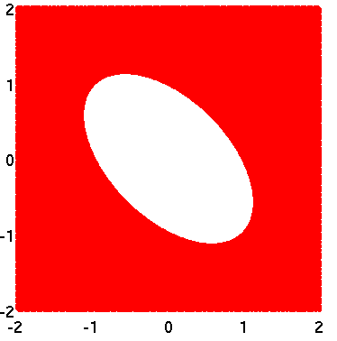
Figure 2. The imaginary projection of $f(z_{1},z_{2})=z_{1}^{2}+z_{2}^{2}+z_{1}z_{2}+z_{1}+z_{2}+1$, intersected with $[-2,2]^{2}$.

The following fact allows to reduce the case of reducible polynomials to the case of irreducible polynomials.

Lemma 3.1.

For $f_{1},f_{2}\in\mathbb{C}[\mathbf{z}]$, we have $\mathcal{I}(f_{1}\cdot f_{2})=\mathcal{I}(f_{1})\cup\mathcal{I}(f_{2})$.

Proof.

By definition of the imaginary projection we have

$$\mathcal{I}(f_{1}\cdot f_{2})\,=\,\operatorname{Im}\mathcal{V}(f_{1}\cdot f_{2})\,=\,\operatorname{Im}(\mathcal{V}(f_{1})\cup\mathcal{V}(f_{2}))\,=\,\operatorname{Im}\mathcal{V}(f_{1})\cup\operatorname{Im}\mathcal{V}(f_{2})\,=\,\mathcal{I}(f_{1})\cup\mathcal{I}(f_{2}).$$

∎

The imaginary projections of affine hyperplanes can be characterized as follows.

Theorem 3.2.

For every affine-linear polynomial $f=a_{0}+\sum_{j=1}^{n}a_{j}z_{j}\in\mathbb{C}[\mathbf{z}]$ with $(a_{1},\ldots,a_{n})\neq{\bf 0}$ the following statements hold.

1. $\mathcal{I}(f)=\begin{cases}\mathcal{V}_{\mathbb{R}}\left(\operatorname{Im}(a_{0}e^{-i\varphi}\right)+\sum\limits_{j=1}^{n}a_{j}e^{-i\varphi}y_{j})\,,&\text{if }a_{0}\in\mathbb{C}\text{ and }(a_{1},\ldots,a_{n})=\mathbf{b}\cdot e^{i\varphi}\\ &\quad\text{ with some }\mathbf{b}\in\mathbb{R}^{n}\text{ and }\varphi\in[0,2\pi)\,.\\ \mathbb{R}^{n}\,,&\text{otherwise.\raisebox{17.22217pt}{\hskip 2.84544pt}}\end{cases}$

2. If all coefficients of $f$ are real, then $f$ is stable if and only if $a_{1},\ldots,a_{n}\geq 0$ or $a_{1},\ldots,a_{n}\leq 0$.

Note that by statement (1), an affine-linear polynomial $f$ cannot be stable if $(a_{1},\ldots,a_{n})\not\in e^{i\varphi}\cdot\mathbb{R}^{n}$, and thus statement (2) provides a complete classification for the stability of an affine-linear polynomial.

Proof.

If all coefficients $a_{1},\ldots,a_{n}$ are real, then

$$\mathcal{I}(f) = \left\{\mathbf{y}\in\mathbb{R}^{n}\,:\,\exists\mathbf{x}\in\mathbb{R}^{n}\;\operatorname{Re}(a_{0})+\sum_{j=1}^{n}a_{j}x_{j}=0\text{ and }\operatorname{Im}(a_{0})+\sum_{j=1}^{n}a_{j}y_{j}=0\right\}$$

$$= \left\{\mathbf{y}\in\mathbb{R}^{n}\,:\,\operatorname{Im}(a_{0})+\sum_{j=1}^{n}a_{j}y_{j}=0\right\}\,,$$

and in the situation $(a_{1},\ldots,a_{n})\in e^{i\varphi}\cdot\mathbb{R}^{n}$, apply the real case to $e^{-i\varphi}f$.

Now assume that $(a_{1},\ldots,a_{n})$ is not a complex multiple of a real vector. That is, the real matrix $\begin{pmatrix}\operatorname{Re}(a_{1})&\cdots&\operatorname{Re}(a_{n})\\ \operatorname{Im}(a_{1})&\cdots&\operatorname{Im}(a_{n})\end{pmatrix}$ has rank 2. By possibly changing the order of the coefficients $a_{j}$, we can assume that the matrix $A=\begin{pmatrix}\operatorname{Re}(a_{1})&\operatorname{Re}(a_{2})\\ \operatorname{Im}(a_{1})&\operatorname{Im}(a_{2})\end{pmatrix}$ is invertible. In order to show $\mathcal{I}(f)=\mathbb{R}^{n}$, consider a fixed $\mathbf{y}\in\mathbb{R}^{n}$ and choose arbitrary $x_{3},\ldots,x_{n}\in\mathbb{R}$. Then the conditions $\operatorname{Re}f(\mathbf{x}+i\mathbf{y})=0$ and $\operatorname{Im}f(\mathbf{x}+i\mathbf{y})=0$ yield a system of two real linear equations in $x_{1},x_{2}$ with coefficient matrix $A$,

$$0 = \operatorname{Re}f(\mathbf{x}+i\mathbf{y})\ =\ \operatorname{Re}a_{0}+\sum_{j=1}^{n}\operatorname{Re}(a_{j})x_{j}-\sum_{j=1}^{n}\operatorname{Im}(a_{j})y_{j}\,,$$

$$0 = \operatorname{Im}f(\mathbf{x}+i\mathbf{y})\ =\ \operatorname{Im}a_{0}+\sum_{j=1}^{n}\operatorname{Im}(a_{j})x_{j}+\sum_{j=1}^{n}\operatorname{Re}(a_{j})y_{j}\,.$$

Since $A$ is invertible and $x_{3},\ldots,x_{n}$ are fixed, there exists a solution $x_{1},x_{2}\in\mathbb{R}$, and thus $\mathbf{y}\in\mathcal{I}(f)$. This completes the proof of (1).

Now let all coefficients of $f$ be real. By part (1), $f$ has a zero with $\operatorname{Im}(z_{j})>0$ for all $j$ if and only if there exists at least one positive coefficient and one negative coefficient. ∎

Corollary 3.3.

Let $n\geq 2$ and $f=a_{0}+\sum_{j=1}^{n}a_{j}z_{j}$ be a stable affine-linear polynomial. Then there exists a (complex) $\varepsilon$-perturbation of the coefficients such that the resulting polynomial is not stable. If all coefficients $a_{0},\ldots,a_{n}$ are real and non-zero then for any real infinitesimal perturbations the stability of $f$ is preserved.

            

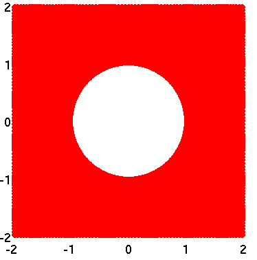
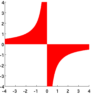
Figure 3. The imaginary projections of $f(z_{1},z_{2})=z_{1}^{2}+z_{2}^{2}+1$ and $f(z_{1},z_{2})=z_{1}z_{2}+z_{1}+z_{2}-1$.

The set $\mathcal{I}(f)$ is not always a closed set. Indeed, already in the quadratic setting all the following cases can occur.

1. $\mathcal{I}(f)$ is open for $f(z_{1},z_{2})=z_{1}^{2}+z_{2}^{2}-1$. In fact, $\mathcal{I}(f)=\mathbb{R}^{n}$.

2. $\mathcal{I}(f)$ is closed for $f(z_{1},z_{2})=z_{1}^{2}+z_{2}^{2}+1$.

3. $\mathcal{I}(f)$ is neither open nor closed for $f(z_{1},z_{2})=z_{1}z_{2}+z_{1}+z_{2}-1$. The hyperbolic curve belongs to $\mathcal{I}(f)$, but, except the origin, the axes do not belong to $\mathcal{I}(f)$.

See Figure 3, and for further details on the specific examples we refer to the discussion of quadratic polynomials in Section 5.

Open problem 3.4.

Let $f\in\mathbb{C}[\mathbf{z}]$ be a polynomial. Is $\mathcal{I}(f)$ open if and only if $\mathcal{I}(f)=\mathbb{R}^{n}$? Clearly, the if-direction is obvious.

Remark 3.5.

If $f$ has real coefficients, then the zeros of $f$ come in conjugated pairs. Therefore, $\mathcal{I}(f)$ is symmetric with respect to the origin.

4. Components of the complement

Similar to amoebas and coamoebas, the complement of an imaginary projection can have several connected components. In contrast to amoebas, already quadratic polynomials can lead to bounded components in the complement. Indeed, the complement of the imaginary projection of $f(z_{1},z_{2})=z_{1}^{2}+z_{2}^{2}+1$ has a bounded component, see Figure 3. The existence of this bounded component of the complement is a consequence of $\operatorname{Re}(f(x_{1}+iy_{1},x_{2}+iy_{2}))=x_{1}^{2}-y_{1}^{2}+x_{2}^{2}-y_{2}^{2}+1$. If $y_{1}^{2}+y_{2}^{2}<1$, then there cannot be any $x_{1},x_{2}\in\mathbb{R}$ with $\operatorname{Re}(f)=0$. Also note that the origin is contained in the complement of an imaginary projection $\mathcal{I}(f)$ whenever $f$ has a real solution.

Set $A^{\mathsf{c}}=\mathbb{R}^{n}\setminus A$ for the complement of a set $A\subset\mathbb{R}^{n}$, and write $\overline{A}$ for the closure of $A$. As pointed out in Section 2.2, it is an important property of amoebas and coamoebas that the components of $\mathcal{A}(f)$ and of $\overline{co\mathcal{A}(f)}$ are convex. As a key property of imaginary projections, we show that the closure their complement consists of convex components as well.

Theorem 4.1.

For every polynomial $f\in\mathbb{C}[\mathbf{z}]$, all components of $\overline{\mathcal{I}(f)}^{\mathsf{c}}$ are convex. The number of these convex components is finite.

Proof.

Let $C$ be a component of the complement of $\overline{\mathcal{I}(f)}$. Define the holomorphic map

$$\psi:\mathbb{C}^{n}\rightarrow\mathbb{C}^{n},\quad\mathbf{z}\mapsto\mathbf{z}\cdot e^{-i\frac{\pi}{2}},$$

which is equivalent to $\textbf{x}+i\textbf{y}\mapsto\textbf{y}-i\textbf{x}$. Furthermore, let

$$C_{\psi}\ =\ \psi(\mathbb{R}^{n}+iC)\ =\ C-i\mathbb{R}^{n}\ =\ C+i\mathbb{R}^{n}.$$

We observe that $C_{\psi}$ is a tubular region, that is, for any $\textbf{y}\in C_{\psi}\cap\mathbb{R}^{n}$ we have $\textbf{y}+i\textbf{x}\in C_{\psi}$ for all $\textbf{x}\in\mathbb{R}^{n}$. Moreover, the function

$$g:C_{\psi}\to\mathbb{C},\quad\textbf{w}\mapsto\frac{1}{f(\psi(\textbf{w}))}$$

is holomorphic on $C_{\psi}$, and $C_{\psi}$ is the maximal tube with this property. By Bochner’s Tube Theorem [4], $g$ is holomorphic on the convex hull of $C_{\psi}$ (considered as set in $\mathbb{R}^{2n}\cong\mathbb{C}^{n}$). Due to the maximality of $C_{\psi}$, this implies the convexity of $C_{\psi}$. Since $C_{\psi}=\psi(\mathbb{R}^{n}+iC)=C+i\mathbb{R}^{n}$, we obtain the convexity of $C$.

As $\mathcal{I}(f)$ is a semialgebraic set, the complement of $\mathcal{I}(f)$ is semialgebraic as well. Then finiteness of the number of convex components follows from the classical bounds of Oleinik-Petrovski or Milnor-Thom, see, e.g., [1, Chapter 7]. ∎

Theorem 4.1 implies the following statement on the unbounded components of the complement.

Corollary 4.2.

Every unbounded component of the complement of the closure of an imaginary projection contains a ray.

Proof.

Let $C$ be an unbounded component of the complement of $\overline{\mathcal{I}(f)}$. Then the convex set $C$ is at least one-dimensional. By well-known results in convex analysis (see [26, Cor. II.8.3.1, Thm. II.8.4]), the relative interior of $C$ has a recession cone which coincides with the recession cone of the closure of $C$, and that recession cone contains a non-zero vector. Hence, $C$ contains a ray. ∎

The left picture in Figure 4 shows the imaginary projection of the polynomial $f(z_{1},z_{2})=z_{1}^{2}+z_{1}^{2}z_{2}+2z_{1}+z_{2}+1$ with its $6$ convex components of the complement. The imaginary projection of a non-constant polynomial is always unbounded, see Section 6. As the two right pictures in Figure 4 show, it is possible that an imaginary projection contains both bounded and unbounded components in the complement.

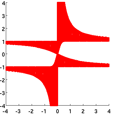
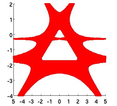
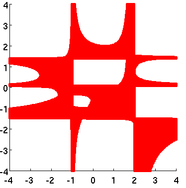
Figure 4. The imaginary projection of $f(z_{1},z_{2})=z_{1}^{2}+z_{1}^{2}z_{2}+2z_{1}+z_{2}+1$, $f(z_{1},z_{2})=z_{1}^{4}+iz_{1}^{3}-z_{1}^{2}z_{2}^{2}+3z_{1}^{2}-2iz_{1}z_{2}^{2}+(4-2i)z_{1}+0.5z_{2}^{2}+1.5$ and of $f(z_{1},z_{2})=z_{1}^{3}z_{2}^{2}-iz_{1}^{3}z_{2}+2z_{1}^{3}-1.8z_{1}^{2}z_{2}-1.8iz_{1}^{2}+2.1z_{1}z_{2}^{2}+2.1iz_{1}z_{2}+4.2z_{1}-0.2iz_{2}^{2}+0.4z_{2}+1.6i$

Corollary 4.3.

For any integers $n>0$ and $t>0$, there exists a polynomial $f\in\mathbb{C}[\mathbf{z}]=\mathbb{C}[z_{1},\ldots,z_{n}]$ such that the complement of $\mathcal{I}(f)$ has exactly $t$ bounded components.

Proof.

We choose an arrangement $\mathcal{H}$ of $d$ hyperplanes $H_{1},\ldots,H_{d}\subseteq\mathbb{R}^{n}$ such that $\mathcal{H}$ has $t$ bounded components of the complement. Using Theorem 3.2, each of the hyperplanes is the imaginary projection of an affine-linear polynomial $f_{1},\ldots,f_{d}\in\mathbb{C}[\mathbf{z}]$. By Lemma 3.1, the imaginary projection of the product of these polynomials gives exactly the hyperplane arrangement. ∎

The proof of Corollary 4.3 constructed $f$ as a product of linear polynomials. In the following, we investigate the imaginary projection of products of linear polynomials in more detail.

Theorem 4.4.

Let $f\in\mathbb{C}[\mathbf{z}]$ be a product of $m$ affine-linear polynomials in $n$ variables. Then the complement of $\mathcal{I}(f)$ consists of at most $\sum_{k=0}^{n}\binom{m}{k}$ components, and this bound is tight.

Proof.

By Theorem 3.2, the imaginary projection of an affine-linear polynomial is either a hyperplane or the whole space $\mathbb{R}^{n}$. We can assume here that the first case holds for every affine-linear polynomial. Then the imaginary projection of the product defines a hyperplane arrangement in $\mathbb{R}^{n}$. If the hyperplanes are in general position, then they decompose the ambient space into exactly $\sum_{k=0}^{n}\binom{m}{k}$ many regions, see [27, Proposition 2.4]. ∎

Theorem 4.4 implies the following lower bound for the maximal number of components of the complement of $\mathcal{I}(f)$ for polynomials $f$ of total degree $d$ in $n$ variables.

Corollary 4.5.

There exists a polynomial $f$ of total degree $d$ in $n$ variables such that the complement of $\mathcal{I}(f)$ consists of exactly $\sum_{k=0}^{n}\binom{d}{k}$ components.

For homogeneous polynomials, the components of the complement are always unbounded since the imaginary projection is a cone. Furthermore, we have the following relation to hyperbolic polynomials.

Theorem 4.6.

Let $f\in\mathbb{R}[\mathbf{z}]$ be homogeneous. Then $\mathcal{I}(f)\neq\mathbb{R}^{n}$ if and only if $f$ is hyperbolic (with respect to some vector $\mathbf{e}\in\mathbb{R}^{n})$.

Proof.

Let $f$ be hyperbolic with respect to $\mathbf{e}\in\mathbb{R}^{n}$. Assuming $\mathbf{e}\in\mathcal{I}(f)$ then implies that for some $\mathbf{x}\in\mathbb{R}^{n}$, the imaginary unit $i$ is a root of the real function $t\mapsto f(\mathbf{x}+t\mathbf{e})$. This is a contradiction to the hyperbolicity of $f$.

Conversely, let $\mathbf{e}\not\in\mathcal{I}(f)$. Then we have $f(\mathbf{x}+i\mathbf{e})\neq 0$ for all $\mathbf{x}\in\mathbb{R}^{n}$, so that in particular

$$f(\mathbf{e})\ =\ (1+i)^{-\deg f}f((1+i)\mathbf{e})\ =\ (1+i)^{-\deg f}f(\mathbf{e}+i\mathbf{e})\neq 0\,.$$

Furthermore, if there exists an $\mathbf{x}\in\mathbb{R}^{n}$ such that $t\mapsto f(\mathbf{x}+t\mathbf{e})$ has a complex solution $a+ib$ with $b\neq 0$, then the homogeneous function $f$ would satisfy

$$f(\mathbf{x}+a\mathbf{e}+ib\mathbf{e})\ =\ 0$$

in contradiction to $\mathbf{e}\not\in\mathcal{I}(f)$. Hence, $f$ is hyperbolic with respect to $\mathbf{e}$. ∎

Similar to Theorem 4.6, for the case of homogeneous polynomials $f\in\mathbb{R}[\mathbf{z}]$, the components of the complement of $\mathcal{I}(f)$ actually coincide with the hyperbolicity cones of $f$ (as defined, e.g., in [14]). The connection between hyperbolicity cones of homogeneous polynomials and imaginary connections are explored further in a follow-up article by the first and the second author [16].

5. Quadratic and multilinear polynomials

In this section, we deal with quadratic and multilinear polynomials. First, we characterize the imaginary projections of quadratic polynomials with real coefficients. The initial two lemmas reduce the problem to the imaginary projections of quadratic polynomials in a normal form.

Lemma 5.1.

Let $f\in\mathbb{C}[\mathbf{z}]$ and $A\in\mathbb{R}^{n\times n}$ be an invertible matrix. Then, $\mathcal{I}(f(A\mathbf{z}))=A^{-1}\mathcal{I}(f(\mathbf{z}))$.

Proof.

Writing $\mathbf{z}=\mathbf{x}+i\mathbf{y}$, the matrix $A$ operates separately on $\mathbf{x}$ and $\mathbf{y}$. Hence,

$$\mathcal{I}(f(A\mathbf{z})) = \{\mathbf{y}\,:\,\exists\mathbf{x}\in\mathbb{R}^{n}\;f(A(\mathbf{x}+i\mathbf{y}))=0\}\ =\ \{A^{-1}\mathbf{y^{\prime}}\,:\,\exists\mathbf{x}^{\prime}\in\mathbb{R}^{n}\;f(\mathbf{x^{\prime}}+i\mathbf{y^{\prime}})=0\}$$

$$= A^{-1}\mathcal{I}(f(\mathbf{z})).$$

∎

Lemma 5.2.

A real translation $\mathbf{z}\mapsto\mathbf{z}+\mathbf{a}$, $\mathbf{a}\in\mathbb{R}^{n}$, does not change the imaginary projection of a polynomial. An imaginary translation $\mathbf{z}\mapsto\mathbf{z}+i\mathbf{a}$, $\mathbf{a}\in\mathbb{R}^{n}$, shifts an imaginary projection in direction $-\mathbf{a}$.

Proof.

The statement holds, since the first kind of transformation just translates the real part of the variables and the second one shifts the imaginary parts of the solutions of $f(\mathbf{z})=0$ in direction $-\mathbf{a}$. ∎

By the Lemmas 5.1 and 5.2, it suffices to study the imaginary projections of polynomials in a normal form in order to understand the imaginary projections of general quadratic polynomials with real coefficients. Every real bivariate quadric is affinely equivalent to a quadric given by one of the following polynomials, where the names come from the conic sections arising from considering these polynomials as real polynomials.

1. $z_{1}^{2}+z_{2}^{2}-1$ (ellipse),

2. $z_{1}^{2}-z_{2}^{2}-1$ (hyperbola),

3. $z_{1}^{2}+z_{2}$ (parabola),

4. $z_{1}^{2}+z_{2}^{2}+1$ (empty set),

or one of the special cases $(v)$ $z_{1}^{2}-z_{2}^{2}$ (pair of crossing lines), $(vi)$ $z_{1}^{2}-1$ (parallel lines, or a single line $z_{1}^{2}$), $(vii)$ $z_{1}^{2}+z_{2}^{2}$ (isolated point), $(viii)$ $z_{1}^{2}+1$ (empty set).

In the following theorem, we characterize the imaginary projections of these quadratic polynomials.

Theorem 5.3.

For a quadratic polynomial $f\in\mathbb{R}[z_{1},z_{2}]$, we have

$$\mathcal{I}(f)\ =\ \begin{cases}\mathbb{R}^{2}&\text{if $f$ is of type $(i)$},\\ \{-1\leq y_{1}^{2}-y_{2}^{2}<0\}\cup\{\mathbf{0}\}&\text{if $f$ is of type $(ii)$},\\ \mathbb{R}^{2}\setminus\{(0,y_{2}):y_{2}\neq 0\}&\text{if $f$ is of type $(iii)$},\\ \{y_{1}^{2}+y_{2}^{2}-1\geq 0\}&\text{if $f$ is of type $(iv)$}.\end{cases}$$

In the cases $(v)$ – $(viii)$, we respectively have $\mathcal{I}(f)=\{\mathbf{y}\in\mathbb{R}^{2}\,:\,y_{1}^{2}-y_{2}^{2}=0\}$, $\mathcal{I}(f)=\{\mathbf{y}\in\mathbb{R}^{2}\,:\,y_{1}=0\}$, $\mathcal{I}(f)=\mathbb{R}^{2}$, and $\mathcal{I}(f)=\{\mathbf{y}\in\mathbb{R}^{2}\,:\,y_{1}=\pm 1\}$.

      

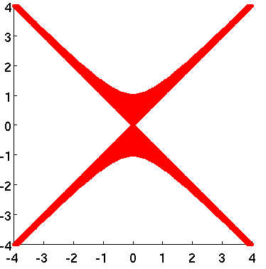
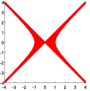
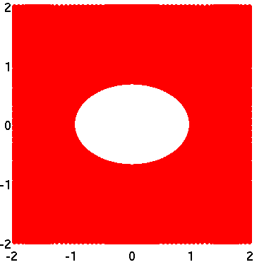
Figure 5. The imaginary projections of $f(z_{1},z_{2})=-z_{1}^{2}+z_{2}^{2}-1$, $f(z_{1},z_{2})=z_{1}^{2}-z_{2}^{2}-1$, and $f(z_{1},z_{2})=2z_{1}^{2}+z_{2}^{2}+1$.

The imaginary projections of some quadratic polynomials are shown in Figure 5, in particular, the middle figure depicts case (ii) from Theorem 5.3.

Proof.

For cases $(i)$–$(ii)$ and $(iv)$–$(viii)$, we consider a polynomial $f=\alpha z_{1}^{2}+\beta z_{2}^{2}+\gamma$ with $\alpha,\beta,\gamma\in\mathbb{R}$. Decomposing $f(\mathbf{z})=0$ into the real and imaginary parts gives $\alpha x_{1}^{2}-\alpha y_{1}^{2}+\beta x_{2}^{2}-\beta y_{2}^{2}+\gamma=0$ and $\alpha x_{1}y_{1}+\beta x_{2}y_{2}=0$. For $y_{1}\neq 0$, eliminating $x_{1}$ shows that

(5.1) $$\mathcal{I}(f)\ =\ \{\textbf{y}\in\mathbb{R}^{n}\,:\,x_{2}^{2}\left(\alpha\beta y_{1}^{2}+\beta^{2}y_{2}^{2}\right)=\alpha y_{1}^{2}(\alpha y_{1}^{2}+\beta y_{2}^{2}-\gamma)\text{ has a real solution $x_{2}$}\}\,.$$

In case $(i)$, we have $\alpha=\beta=1$, $\gamma=-1$, which altogether gives $\mathcal{I}(f)=\mathbb{R}^{2}$. In case $(ii)$, we have $\alpha=1$, $\beta=\gamma=-1$. For $y_{1}\neq 0$, real solutions for $x_{2}$ in (5.1) exist for $0<y_{2}^{2}-y_{1}^{2}<1$ as well as in the special case $y_{1}^{2}-y_{2}^{2}+1=0$. And for $y_{1}=0$, we obtain $\mathbf{y}\in\mathcal{I}(f)$ if and only if $y_{2}^{2}\leq 1$.

Cases $(iv)$–$(viii)$ can be treated similarly. Finally, case $(iii)$ is linear in $z_{2}$, so that the equations for the real and imaginary part can be solved directly for $x_{2}$ and $y_{2}$. ∎

Now we deal with quadrics in $n$-dimensional space. Since every quadric in $\mathbb{R}^{n}$ is affinely equivalent to a quadric given by one of the following polynomials,

$$\begin{array}[]{cll}\text{(I)}&\sum_{j=1}^{p}z_{j}^{2}-\sum_{j=p+1}^{r}z_{j}^{2}&\quad(1\leq p\leq r,\,r\geq 1,\,p\geq\frac{r}{2})\,,\\ \text{(II)}&\sum_{j=1}^{p}z_{j}^{2}-\sum_{j=p+1}^{r}z_{j}^{2}+1&\quad(0\leq p\leq r,\,r\geq 1)\,,\\ \text{(III)}&\sum_{j=1}^{p}z_{j}^{2}-\sum_{j=p+1}^{r}z_{j}^{2}+z_{r+1}&\quad(1\leq p\leq r,\,r\geq 1,\,p\geq\frac{r}{2})\,,\end{array}$$

it suffices to discuss these cases. (See, e.g., [2] as a general background reference for real quadrics.)

Theorem 5.4.

Let $n\geq r\geq 3$ and $f\in\mathbb{R}[\mathbf{z}]$ be a quadratic polynomial.

1. If $f$ is of type $\mathrm{(I)}$, then

   (5.2) $$\mathcal{I}(f)\ =\ \begin{cases}\mathbb{R}^{n}&\text{if }\frac{r}{2}\leq p<r-1\text{ or }p=r\,,\\ \{\mathbf{y}\in\mathbb{R}^{n}\;:\,y_{r}^{2}\leq\sum_{j=1}^{r-1}y_{j}^{2}\}&\text{if }p=r-1\,.\end{cases}$$

2. If $f$ is of type $\mathrm{(II)}$, then

   (5.3) $$\mathcal{I}(f)\ =\ \begin{cases}\mathbb{R}^{n}&\text{if }p=0\text{ or }1<p<r-1\,,\\ \{\mathbf{y}\in\mathbb{R}^{n}\;:\,y_{1}^{2}-\sum_{j=2}^{r}y_{j}^{2}\leq 1\}&\text{if }p=1\,,\\ \{\mathbf{y}\in\mathbb{R}^{n}\;:\,\sum_{j=1}^{r-1}y_{j}^{2}>y_{r}^{2}\}\cup\{\mathbf{0}\}&\text{if }p=r-1\,,\\ \{\mathbf{y}\in\mathbb{R}^{n}\;:\,\sum_{j=1}^{r}y_{j}^{2}\geq 1\}&\text{if }p=r\,.\end{cases}$$

3. If $n>r$ and $f$ is of type $\mathrm{(III)}$, then

   $$\mathcal{I}(f)\ =\ \mathbb{R}^{n}\setminus\{(0,\ldots,0,y_{r+1},y_{r+2},\ldots,y_{n})\,:\,y_{r+1}\neq 0,\,y_{r+2},\ldots,y_{n}\in\mathbb{R}\}.$$

Note that the case $n\geq 3$ differs significantly from $n=2$. The proof of Theorem 5.4 is given in the Lemmas 5.5–5.7.

Lemma 5.5.

Let $n\geq r\geq 3$. If $f(\mathbf{z})=\sum_{j=1}^{p}z_{j}^{2}-\sum_{j=p+1}^{r}z_{j}^{2}$ with $\frac{r}{2}<p\leq r$, then $\mathcal{I}(f)$ is given by (5.2).

Proof.

Without loss of generality we can assume $r=n$. Splitting the problem into the real and imaginary part yields

(5.4) $$\sum_{j=1}^{p}x_{j}^{2}-\sum_{j=p+1}^{n}x_{j}^{2}-\sum_{j=1}^{p}y_{j}^{2}+\sum_{j=p+1}^{n}y_{j}^{2} = 0\,,$$

(5.5) $$\sum_{j=1}^{p}x_{j}y_{j}-\sum_{j=p+1}^{n}x_{j}y_{j} = 0\,.$$

Consider a fixed $\textbf{y}\in\mathbb{R}^{n}$. If $-\sum_{j=1}^{p}y_{j}^{2}+\sum_{j=p+1}^{n}y_{j}^{2}=0$, then $x_{1}=\cdots=x_{n}=0$ gives a solution to (5.4) and (5.5). Therefore, we can assume $-\sum_{j=1}^{p}y_{j}^{2}+\sum_{j=p+1}^{n}y_{j}^{2}\neq 0$.

In the case $p=n$, by reordering the indices, we can assume that $y_{1}^{2}+y_{2}^{2}\neq 0$, and choose $\textbf{x}=\frac{\|\textbf{y}\|_{2}}{(y_{1}^{2}+y_{2}^{2})^{1/2}}(-y_{2},y_{1},0,\ldots,0)$ to obtain a solution for (5.4) and (5.5).

In the case $p=n-1$, the $n$-dimensional hyperboloid (5.4) in the $x$-variables is one-sheeted for $-\sum_{j=1}^{n-1}y_{j}^{2}+y_{n}^{2}<0$ and two-sheeted for $-\sum_{j=1}^{n-1}y_{j}^{2}+y_{n}^{2}>0$. In case of a one-sheeted hyperboloid, its intersection with the hyperplane (5.5) is never empty. Namely, choosing $x_{3}=\cdots=x_{n-1}=0$, gives the hyperboloid $x_{1}^{2}+x_{2}^{2}-x_{n}^{2}=\sum_{j=1}^{n-1}y_{j}^{2}-y_{n}$ in $x_{1},x_{2},x_{n}$, that contains the origin in the inner component of its complement.

Now consider the case where the hyperboloid consists of two sheets. For any $\alpha>0$, the sets $\{\mathbf{y}\in\mathbb{R}^{n}\,:\,-\sum_{j=1}^{n-1}y_{j}^{2}+y_{n}^{2}=\alpha>0\}$ and $\{\mathbf{x}\in\mathbb{R}^{n}\,:\,\sum_{j=1}^{n-1}x_{j}^{2}-x_{n}^{2}=-\alpha\}$ coincide. Furthermore, after a coordinate transformation we can assume $\alpha=1$ and set $H=\{\mathbf{x}\in\mathbb{R}^{n}\,:\,-\sum_{j=1}^{n-1}x_{j}^{2}+x_{n}^{2}=1\}$.

We claim that the intersection of $H$ with the hyperplane (5.5) is always empty. Due to the symmetry of $H$ with respect to all the coordinate hyperplanes $x_{k}=0$ for $1\leq k\leq n-1$, it suffices by (5.5) to show that the hyperboloid $H$ does not contain two distinct points, whose position vectors are orthogonal to each other with respect to the Euclidean scalar product. Because of the rotational symmetry of $H$ with regard to the $x_{n}$-axis and the invariance of scalar products under orthogonal transformations, by applying an orthogonal transformation it suffices to consider the situation $x_{2}=\cdots=x_{n-1}=0$. The resulting hyperbola $-x_{1}^{2}+x_{n}^{2}=1$ in the $x_{1}$-$x_{n}$-plane has no two orthogonal position vectors. Namely, the asymptotes $x_{1}=\pm x_{n}$ divide the plane into four quarters, and the hyperbola is contained in the strict interiors of two opposite quarters.

Now consider the case $\frac{n}{2}<p<n-1$. By our initial considerations in the proof, we have already covered the case $\mathbf{y}=\mathbf{0}$. In the case $\mathbf{y}\neq\mathbf{0}$, by changing the coordinates we can assume that $(y_{1},y_{2},y_{p+1})$ is not the zero vector. Choose $(x_{p+2},\ldots,x_{n})\in\mathbb{R}^{n-p-1}$ such that $-\sum_{j=p+2}^{n}x_{j}^{2}-\sum_{j=1}^{p}y_{j}^{2}+\sum_{j=p+1}^{n}y_{j}^{2}=:\alpha<0$. Then, since $\mathbf{y}$ is fixed, (5.4) becomes a hyperboloid of one sheet and (5.5) becomes an affine hyperplane. The intersection of these two hypersurfaces is non-empty. Namely, choosing $x_{3}=\cdots=x_{p}=0$, gives the one-sheeted hyperboloid $\{(x_{1},x_{2},x_{p+1})\in\mathbb{R}^{3}\,:\,x_{1}^{2}+x_{2}^{2}-x_{p+1}^{2}=-\alpha>0\}$, which intersects the affine hyperplane with normal vector $(y_{1},y_{2},-y_{p+1})$ and constant term $-\sum_{j=p+2}^{n}x_{j}y_{j}$. Hence, there exists an $\mathbf{x}\in\mathbb{R}^{n}$ satisfying (5.4) and (5.5). ∎

Lemma 5.6.

Let $n\geq r\geq 3$ and $f(\mathbf{z})=\sum_{j=1}^{p}z_{j}^{2}-\sum_{j=p+1}^{r}z_{j}^{2}+1$ with $0\leq p\leq r$.

1. If $p=0$ then $\mathcal{I}(f)=\mathbb{R}^{n}$.

2. If $p=1$ then $\mathcal{I}(f)=\{\mathbf{y}\in\mathbb{R}^{n}\,:\,y_{1}^{2}-\sum_{j=2}^{r}y_{j}^{2}\leq 1\}$.

3. If $1<p<r-1$ then $\mathcal{I}(f)=\mathbb{R}^{n}$.

4. If $p=r-1$ then $\mathcal{I}(f)=\{\mathbf{y}\in\mathbb{R}^{n}\;:\,\sum_{j=1}^{r-1}y_{j}^{2}>y_{r}^{2}\}\cup\{\mathbf{0}\}$.

5. If $p=r$ then $\mathcal{I}(f)=\{\mathbf{y}\in\mathbb{R}^{n}\,:\,\sum_{j=1}^{r}y_{j}^{2}\geq 1\}$.

Note that for $r=3$ the case (3) cannot occur.

Proof.

Similar to the proof of Lemma 5.5, we can assume $r=n$ and split the problem into the real and imaginary part,

(5.6) $$\sum_{j=1}^{p}x_{j}^{2}-\sum_{j=p+1}^{n}x_{j}^{2}-\sum_{j=1}^{p}y_{j}^{2}+\sum_{j=p+1}^{n}y_{j}^{2}+1 = 0\,,$$

(5.7) $$\sum_{j=1}^{p}x_{j}y_{j}-\sum_{j=p+1}^{n}x_{n}y_{n} = 0\,.$$

Consider a fixed $\textbf{y}\in\mathbb{R}^{n}$.

In the case $p=0$, we obtain the two equations $\sum_{j=1}^{n}x_{j}^{2}=\sum_{j=1}^{n}y_{j}^{2}+1$ and $\sum_{j=1}^{n}x_{j}y_{j}=0$. Setting $\textbf{x}=\big{(}\frac{\|\textbf{y}\|_{2}^{2}+1}{y_{1}^{2}+y_{2}^{2}}\big{)}^{1/2}(-y_{2},y_{1},0,\ldots,0)$ gives a solution.

In the case $p=1$, set $\alpha=-y_{1}^{2}+\sum_{j=2}^{n}y_{j}^{2}+1$. Then the statement follows identically as in Lemma 5.5 in the cases $\alpha=0$, $\alpha<0$ and $\alpha>0$. For $\alpha=0$, the point $\mathbf{x}=\mathbf{0}$ is a solution for $f(\mathbf{z})=f(\mathbf{x}+i\mathbf{y})=0$. For $\alpha>0$, (5.6) is a one-sheeted hyperboloid and (5.7) is a hyperplane. Their intersection is non-empty. For $\alpha<0$, the formula for $\alpha$ and (5.6) both define two-sheeted hyperboloids. We consider the hyperboloids $H_{1}:=\{\mathbf{y}\in\mathbb{R}^{n}\,:\,y_{1}^{2}-\sum_{j=2}^{n}y_{j}^{2}=1-\alpha\}$ and $H_{2}:=\{\mathbf{x}\in\mathbb{R}^{n}\,:\,x_{1}^{2}-\sum_{j=2}^{n}x_{j}^{2}=-\alpha\}$. Via the transformations $\mathbf{y}\mapsto\mathbf{y}/\sqrt{1-\alpha}$ and $\mathbf{x}\mapsto\mathbf{x}/\sqrt{-\alpha}$ these sets are transformed into the same set $C=\{\mathbf{x}\in\mathbb{R}^{n}\,:\,x_{1}^{2}-\sum_{j=2}^{n}x_{j}^{2}=1\}$. We know by the proof of Lemma 5.5 that there is no pair of orthogonal position vectors on $C$. Therefore, there are no orthogonal position vectors in $H_{1}$ and $H_{2}$. Hence, for $\alpha<0$ the equation $f(\mathbf{z})=0$ has no solution in $\mathbf{x}$. The case $p=r-1$ is similar.

In the case $1<p<r-1$, the statement follows as in Lemma 5.5.

In the case $p=n$, there exists an x satisfying  (5.6) and (5.7) if and only if $\sum_{j=1}^{n}y_{j}^{2}-1\geq 0$. ∎

Lemma 5.7.

Let $n>r\geq 2$. If $f(\mathbf{z})=\sum_{j=1}^{p}z_{j}^{2}-\sum_{j=p+1}^{r}z_{j}^{2}+z_{r+1}$ with $1\leq p\leq r$, then $\mathcal{I}(f)=\mathbb{R}^{n}\setminus\{(0,\ldots,0,y_{r+1},y_{r+2},\ldots,y_{n})\,:\,y_{r+1}\neq 0,\,y_{r+2},\ldots,y_{n}\in\mathbb{R}\}$.

Proof.

We can assume $n=r+1$. In the system for the real and the imaginary parts

(5.8) $$\sum_{j=1}^{p}x_{j}^{2}-\sum_{j=p+1}^{n-1}x_{j}^{2}-\sum_{j=1}^{p}y_{j}^{2}+\sum_{j=p+1}^{n-1}y_{j}^{2}+x_{n}=0\ ,$$

(5.9) $$2\sum_{j=1}^{p}x_{j}y_{j}-2\sum_{j=p+1}^{n-1}x_{j}y_{j}+y_{n}=0\ ,$$

consider a fixed $(y_{1},\ldots,y_{n})\in\mathbb{R}^{n}$. If $(y_{1},\ldots,y_{n-1})\neq\mathbf{0}$, then we can choose $(x_{1},\ldots,x_{n-1})\in\mathbb{R}^{n}$ such that (5.9) is satisfied. Since (5.8) is linear in $x_{n}$, it has a real solution for $x_{n}$. In the special case $(y_{1},\ldots,y_{n-1})=\mathbf{0}$, we see that $\mathbf{y}=(y_{1},\ldots,y_{n})\in\mathcal{I}(f)$ if and only if $y_{n}=0$. ∎

Lemmas 5.1 and 5.2 also provide a statement about the existence of unbounded components in the complement.

Theorem 5.8.

Let $f\in\mathbb{C}[\mathbf{z}]$.

1. The complement of $\mathcal{I}(f)$ contains the non-negative $y_{1}$-axis $\mathbb{R}_{\geq 0}\times\{0\}^{n-1}$ if and only if the polynomial $f(z_{1}+ir,z_{2},\ldots,z_{n})$ has no real solution in $\mathbf{z}$ for any $r\geq 0$.

2. $\overline{\mathcal{I}(f)}$ has an unbounded component in the complement if and only if there is an affine transformation $\mathbf{z}\mapsto A\mathbf{z}+i\mathbf{b}$ with a real matrix $A$ and a real vector $\mathbf{b}$ such that condition $(1)$ is satisfied.

Proof.

The first statement immediately follows from the definition of $\mathcal{I}(f)$. For the second statement, Corollary 4.2 implies that the existence of an unbounded component in the complement is equivalent to the existence of a ray in the complement. By the Lemmas 5.1 and 5.2, the affine transformation reduces the situation to (1). ∎

Multilinear polynomials

We study the imaginary projection of multilinear polynomials (in the sense of multi-affine-linear). Brändén’s stability result for this class was given in Theorem 2.5. The next statement describes the imaginary projection of bivariate multilinear polynomials; see the right picture in Figure 3 for an example.

Theorem 5.9.

Let $f(z_{1},z_{2})=z_{1}z_{2}+\beta z_{1}+\gamma z_{2}+\delta$ be a multilinear polynomial with $\beta,\gamma,\delta\in\mathbb{R}$. Then

$$\mathcal{I}(f)\ =\ \Big{\{}\mathbf{y}\in\mathbb{R}^{2}\,:\,0<\frac{y_{1}y_{2}}{\delta-\beta\gamma}\leq 1\Big{\}}\cup\{\mathbf{0}\}\qquad\text{for }\delta-\beta\gamma\,\neq\,0\,.$$

In the special case $\delta=\beta\gamma$, the multilinear polynomial is reducible and thus $\mathcal{I}(f)=\mathcal{I}(z_{1}+\gamma)\cup\mathcal{I}(z_{2}+\beta)=\mathcal{I}(z_{1})\cup\mathcal{I}(z_{2})=(\mathbb{R}\times\{0\})\cup(\{0\}\times\mathbb{R})$.

As a consequence, we rediscover that the multilinear polynomial $f$ is stable if and only if $\beta\gamma-\delta\geq 0$, see Theorem 2.5.

Proof.

Since $f$ can be written as $f(z_{1},z_{2})=(z_{1}+\gamma)(z_{2}+\beta)+\delta-\beta\gamma$, Lemma 5.2 implies that $\mathcal{I}(f)=\mathcal{I}(g)$ where $g(z_{1},z_{2})=z_{1}z_{2}+\delta-\beta\gamma$. Substituting $z_{1}=z_{1}^{\prime}+z_{2}^{\prime}$ and $z_{2}=(\beta\gamma-\delta)(z_{1}^{\prime}-z_{2}^{\prime})$, we can express $g$ as $g(z_{1}^{\prime},z_{2}^{\prime})=(\beta\gamma-\delta)(z_{1}^{2}-z_{2}^{2}-1)$, and by Theorem 5.3, the imaginary projection of $g$ with respect to the $\mathbf{z^{\prime}}$-variables is

$$\{\mathbf{y^{\prime}}\in\mathbb{R}^{2}\,:\,-1\leq(y^{\prime}_{1})^{2}-(y^{\prime}_{2})^{2}<0\}\cup\{\mathbf{0}\}\,.$$

Using $\begin{pmatrix}1&1\\ \beta\gamma-\delta&-(\beta\gamma-\delta)\end{pmatrix}^{-1}=\frac{1}{2}\begin{pmatrix}1&1/(\beta\gamma-\delta)\\ 1&-1/(\beta\gamma-\delta)\end{pmatrix}$, transforming back to the $\mathbf{z}$-variables with Lemma 5.1 yields the claim. ∎

For the case of $n$-dimensional multilinear polynomials, we provide the subsequent, less explicit, characterization of the imaginary projection, and more generally, of polynomials of the form $f=g+z_{n+1}h\in\mathbb{C}[\mathbf{z},z_{n+1}]$ with $g,h\in\mathbb{C}[\mathbf{z}]$.

Lemma 5.10.

Let $f=g+z_{n+1}h\in\mathbb{C}[\mathbf{z},z_{n+1}]$ and $v\in\mathbb{R}$. A point $(\mathbf{z},z_{n+1})$ with $\operatorname{Im}z_{n+1}=v$ and $h(\mathbf{z})\neq 0$ is contained in $\mathcal{V}(f)$ if and only if the determinant

(5.10) $$\det\left(\begin{matrix}\operatorname{Re}g-v\operatorname{Im}h&\operatorname{Re}h\\ \operatorname{Im}g+v\operatorname{Re}h&\operatorname{Im}h\end{matrix}\right)$$

vanishes in $\mathbf{z}$.

Proof.

Writing $z_{n+1}=u+iv$, the conditions $\operatorname{Re}f=0$ and $\operatorname{Im}f=0$ give

$$\left(\begin{matrix}\operatorname{Re}g\\ \operatorname{Im}g\end{matrix}\right)+\left(\begin{matrix}\operatorname{Re}h&-\operatorname{Im}h\\ \operatorname{Im}h&\operatorname{Re}h\end{matrix}\right)\left(\begin{matrix}u\\ v\end{matrix}\right)=\left(\begin{matrix}\operatorname{Re}g-v\operatorname{Im}h\\ \operatorname{Im}g+v\operatorname{Re}h\end{matrix}\right)+u\left(\begin{matrix}\operatorname{Re}h\\ \operatorname{Im}h\end{matrix}\right)\ =\ \mathbf{0}\,.$$

Considering this equation as a linear equation in $u$ shows that there exists a solution if and only if the coefficient vector and the constant vector are linearly dependent, that is, if and only the determinant (5.10) vanishes. ∎

We obtain the following corollary.

Corollary 5.11.

Let $f=g+z_{n+1}h\in\mathbb{C}[\mathbf{z},z_{n+1}]$. Then, writing $\mathbf{z}=\mathbf{x}+i\mathbf{y}$, the sets $\mathcal{I}(g+z_{n+1}h)$ and

(5.11) $$\left\{(\mathbf{y},v)\in\mathbb{R}^{n+1}\,:\,\exists\mathbf{x}\in\mathbb{R}^{n}\text{ with }\,\det\left(\begin{matrix}\operatorname{Re}g-v\operatorname{Im}h&\operatorname{Re}h\\ \operatorname{Im}g+v\operatorname{Re}h&\operatorname{Im}h\end{matrix}\right)=0\right\}$$

coincide outside of the exceptional set $E=\{\operatorname{Im}((\mathbf{z},z_{n+1}))\,:\,h(\mathbf{z})=0\text{ and }g(\mathbf{z})\neq 0\}$.

We observe that the determinantal condition in (5.10) and (5.11) gives a linear condition in $v$. For a multilinear polynomial of the form $f=g+z_{n+1}h\in\mathbb{R}[\mathbf{z},z_{n+1}]$ with $g$ and $h$ multilinear, the condition is quadratic in any of the variables $\mathbf{x}=(x_{1},\ldots,x_{n})$ and $\mathbf{y}=(y_{1},\ldots,y_{n})$.

Example 5.12.

We revisit the multilinear polynomial $f(z_{1},z_{2})=z_{1}z_{2}+\delta$, $\delta\in\mathbb{R}\setminus\{0\}$ to illustrate Corollary 5.11; see Theorem 5.9. Setting $g=\delta$ and $h=z_{1}$, the determinantal condition (5.10) gives (where we write $y_{2}$ instead of $v$)

$$\delta y_{1}-y_{1}^{2}y_{2}-x_{1}^{2}y_{2}\ =\ 0\,.$$

For $y_{2}\neq 0$, there exists a real solution for $x_{1}$ if and only if $\frac{y_{1}}{y_{2}}(\delta-y_{1}y_{2})\geq 0$. Taking into account the exceptional set $E=\{0\}\times\mathbb{R}$, we obtain $\mathcal{I}(f)=\{\mathbf{y}\in\mathbb{R}^{2}\,:\,0<\frac{y_{1}y_{2}}{\delta}\leq 1\}\cup\{\mathbf{0}\}$, in accordance with Theorem 5.9.

Example 5.13.

We consider the non-multilinear polynomial $f(z_{1},z_{2})=1+z_{2}z_{1}^{2}$, which is of the form $f=g+z_{2}h$ with $g=1$ and $h=z_{1}^{2}$. Corollary 5.11 gives the quartic condition in the variable $x_{1}$

(5.12) $$-y_{2}x_{1}^{4}-2y_{1}^{2}y_{2}x_{1}^{2}+2y_{1}x_{1}-y_{2}y_{1}^{4}\ =\ 0\,.$$

Recall that the discriminant of a general polynomial $p(z)=\sum_{j=0}^{n}a_{j}z^{j}$ is given by $\operatorname{Disc}(p)=(-1)^{\frac{1}{2}n(n-1)}\frac{1}{a_{n}}\operatorname{Res}(p,p^{\prime})$, where $\operatorname{Res}$ denotes the resultant. For a quartic, a positive discriminant corresponds to zero or four real roots, while a negative discriminant corresponds to two real roots. Moreover, with the notation

$$H\ =\ 8a_{2}a_{4}-3a_{3}^{2}\,,\quad I\ =\ 12a_{0}a_{4}-3a_{1}a_{3}+a_{2}^{2}\,,$$

the case of four real roots corresponds to $H\leq 0$ and $H^{2}-16a_{4}^{2}I\geq 0$, while the case of four complex roots corresponds to $H>0$ or $H^{2}-16a_{4}^{2}I<0$, see, e.g., [9, Proposition 7]. In our situation, $p=p(x_{1})$ is the polynomial in (5.12), $\operatorname{Disc}(p)=16(64y_{1}^{4}y_{2}^{2}-27)y_{1}^{4}y_{2}^{2}$, $H=16y_{1}^{2}y_{2}^{2}$ and $H^{2}-16a_{4}^{2}I=0$. The set of points $\mathbf{y}\in\mathbb{R}^{2}$, where (5.12) has at least two real solutions in $x_{1}$, is given by $64y_{1}^{4}y_{2}^{2}\leq 27$. Taking into account the exceptional set $E=\{0\}\times\mathbb{R}$ gives

$$\mathcal{I}(f)\ =\ \{\mathbf{y}\in\mathbb{R}^{2}\,:\,0<64y_{1}^{4}y_{2}^{2}\leq 27\}\cup(\mathbb{R}\times\{0\})\,.$$

We will return to multilinear polynomials when studying their asymptotic geometry in Theorem 6.3.

6. The limit set of imaginary projections

For the amoeba $\mathcal{A}(f)$ of a polynomial $f$ it is well-known that the set of limit points of points in $\frac{1}{r}\mathcal{A}(f)\cap\mathbb{S}^{n-1}$, where $r>0$ tends to infinity, is a spherical polyhedral complex. It is called the logarithmic limit set

$$\mathcal{A}_{\infty}(f)\ =\ \lim_{r\rightarrow\infty}\left(\frac{1}{r}\mathcal{A}(f)\cap\mathbb{S}^{n-1}\right)$$

and provides one way of defining a tropical hypersurface; see, e.g., [18, Section 1.4].

For imaginary projections, the situation is different from amoebas, as shown by the following counterexample: For $f\in\mathbb{C}[\mathbf{z}]$,

$$\mathcal{I}_{\infty}(f)\ =\ \lim_{r\rightarrow\infty}\left(\frac{1}{r}\mathcal{I}(f)\cap\mathbb{S}^{n-1}\right)$$

is not a spherical polyhedral complex in general.

Example 6.1.

Let $f(\mathbf{z})=z_{1}^{2}-\sum_{j=2}^{n}z_{j}^{2}+1$ with $n\geq 3$. Then, by Theorem 5.4,

$$\mathcal{I}(f)\ =\{\mathbf{y}\in\mathbb{R}^{n}\,:\,y_{1}^{2}-\sum_{j=2}^{n}y_{j}^{2}\leq 1\}\,.$$

Therefore, $\mathcal{I}_{\infty}(f)=\lim_{r\to\infty}\big{\{}\mathbf{y}\in\mathbb{S}^{n-1}\,:\,(ry_{1})^{2}-\sum_{j=2}^{n}(ry_{j})^{2}\leq 1\big{\}}$ can be written as

$$\mathcal{I}_{\infty}(f)\ =\ \Big{\{}\mathbf{y}\in\mathbb{S}^{n-1}\,:\,y_{1}^{2}\leq\sum_{j=2}^{n}y_{j}^{2}\Big{\}}\ =\ \Big{\{}\mathbf{y}\in\mathbb{S}^{n-1}\,:\,y_{1}^{2}\leq\frac{1}{2}\Big{\}}\,.$$

Since $n\geq 3$, this cannot be written as the intersection of $\mathbb{S}^{n-1}$ with a polyhedral fan. Hence, $\mathcal{I}_{\infty}(f)$ is not a spherical polyhedral complex, and since $\mathcal{I}_{\infty}(f)$ is already closed, this persists under taking the closure.

Definition 6.2.

Let $f\in\mathbb{C}[\mathbf{z}]$. We call a point $p\in\mathbb{R}^{n}$ a limit direction of the imaginary projection of $f$ if $p\in\mathcal{I}_{\infty}(f)$.

Unless $f$ is univariate or constant, $f$ has at least one limit direction. Namely, for any integer $N>0$ and $(z_{1},\ldots,z_{n-1})\in\mathbb{C}^{n-1}$ such that $\|(\operatorname{Im}(z_{1}),\ldots,\operatorname{Im}(z_{n-1}))\|_{2}>N$ and $f(z_{1},\ldots,z_{n-1},z_{n})\in\mathbb{C}[z_{n}]$ is not a non-zero constant, there exists a $z_{n}\in\mathbb{C}$ with $f(z_{1},\ldots,z_{n-1},z_{n})=0$. The resulting sequence of points $\mathbf{z}_{N}$ induces a sequence of points $\operatorname{Im}(\mathbf{z}_{N})/\|\operatorname{Im}(\mathbf{z}_{N})\|$ on the unit sphere $\mathbb{S}^{n-1}$. By compactness, there exists a convergent subsequence. If $f$ has real coefficients, then, by Remark 3.5, the limit directions are symmetric with respect to the origin.

In Theorem 6.3 and Corollary 6.4, we deal with the limit directions of multilinear polynomials. Then, in Theorem 6.5 and Corollary 6.7, we provide criteria for one-dimensional families of limit directions, which means in the case $n=2$ that every point on $\mathbb{S}^{1}$ is a limit direction of the imaginary projection.

Theorem 6.3.

Let $f\in\mathbb{C}[\mathbf{z}]$ be a multilinear polynomial, and assume that the monomial $z_{1}\cdots z_{n}$ appears in $f$, i.e., $\deg(f)=n$. Then the limit directions of $\mathcal{I}(f)$ are given by $\mathbb{S}^{n-1}\cap\mathcal{H}$, where $\mathcal{H}$ is the union of the $n$ coordinate hyperplanes $\{\mathbf{y}\in\mathbb{R}^{n}\,:\,y_{j}=0\}$, $1\leq j\leq n$.

Proof.

Homogenizing $f$ to $f_{h}(z_{0},z_{1},\ldots,z_{n})$, the homogeneous polynomial $f_{h}$ has a zero at infinity, i.e., $(0,z_{1},\ldots,z_{n})\in\mathcal{V}(f_{h})$, if and only if $z_{1}\cdots z_{n}=0$. Hence, the set of limit points of points in $\frac{1}{r}\mathcal{V}(f)$, $r\to\infty$, is $\mathcal{V}(z_{1}\cdots z_{n})$. The imaginary projections of the $n$ hyperplanes $\{\mathbf{z}\in\mathbb{C}^{n}\,:\,z_{j}=0\}$ then imply the claim. ∎

Theorem  6.3 allows one to characterize the number of unbounded components in the complement of the imaginary projection of multilinear polynomials.

Corollary 6.4.

Let $f\in\mathbb{C}[\mathbf{z}]$ be a multilinear polynomial, and assume that the monomial $z_{1}\cdots z_{n}$ appears in $f$, i.e., $\deg(f)=n$. Then the complement of $\mathcal{I}(f)$ contains exactly $2^{n}$ unbounded components.

We remark that this number coincides with the number stated in Theorem 4.4 when choosing $m=n$.

Proof.

By Theorem 6.3, the complement of $\mathcal{I}_{\infty}(f)$ consists of $2^{n}$ components. Therefore, the complement of $\mathcal{I}(f)$ has exactly $2^{n}$ unbounded components. ∎

Theorem 6.5.

Let $f\in\mathbb{C}[\mathbf{z}]$ be a non-constant polynomial. If its homogenization $f_{h}\in\mathbb{C}[z_{0},\mathbf{z}]$ has a zero $\mathbf{p}_{h}=(0:p)=(0:p_{1}:\cdots:p_{n})\in\mathbb{P}_{\mathbb{C}}^{n}$, then every point in the intersection $\mathbb{S}^{n-1}\cap\mathcal{H}$ is a limit direction, where $\mathcal{H}=\{\lambda\operatorname{Re}(\mathbf{p})+\mu\operatorname{Im}(\mathbf{p}):\lambda,\mu\in\mathbb{R}\}$ and $\mathbf{p}=(p_{1},\ldots,p_{n})$.

Proof.

Let $\mathbf{p}_{h}=(0:p_{1}:\cdots:p_{n})$ be a zero at infinity of $f_{h}$. Since $i\mathbf{p}_{h}$ is also a point at infinity for $f_{h}$, we can assume that $\sum_{j=1}^{n}\operatorname{Im}(p_{j})^{2}\neq 0$. Since $f$ is non-constant, there exists a sequence $(\mathbf{p}^{(k)})=(p_{1}^{(k)},\ldots,p_{n}^{(k)})$ of points in $\mathcal{V}(f)$ such that $(1:p_{1}^{(k)}:\cdots:p_{n}^{(k)})$ converges to $\mathbf{p}_{h}$. Hence,

$$\frac{1}{(\sum_{j=1}^{n}\operatorname{Im}(p_{j})^{2})^{1/2}}(\operatorname{Im}p_{1},\ldots,\operatorname{Im}p_{n})$$

is a limit direction. Multiplying $\mathbf{p}_{h}$ with a complex number $\mu+i\lambda$, $\lambda,\mu\in\mathbb{R}$ keeps $\mathbf{p}_{h}$ invariant, and under the imaginary projection it leads to a projected point $\operatorname{Im}((\mu+i\lambda)\cdot\mathbf{p})=\mu\operatorname{Im}(\mathbf{p})+\lambda\operatorname{Re}(\mathbf{p})$. Considering all complex numbers $\mu+i\lambda\in\mathbb{C}$, these points form the subspace $\mathcal{H}$. ∎

Example 6.6.

We revisit the polynomial $f(z_{1},z_{2})=z_{1}^{2}-z_{2}^{2}-1$; see Figure 5 for its imaginary projection. Its homogenization is $f_{h}(z_{0},z_{1},z_{2})=z_{1}^{2}-z_{2}^{2}-z_{3}^{2}$ whose zeros at infinity are given by the equation $z_{1}^{2}-z_{2}^{2}=(z_{1}+z_{2})(z_{1}-z_{2})=0$. For the points $\mathbf{p}_{h}=(0:1:\pm 1)$, Theorem 6.5 provides the two one-dimensional lines $\mathcal{H}_{1,2}=\{\lambda(1,\pm 1):\lambda\in\mathbb{R}\}$. We obtain the intersection $\mathbb{S}^{1}\cap\mathcal{H}_{1,2}=\{(\pm\frac{1}{\sqrt{2}},\pm\frac{1}{\sqrt{2}})\}$. Indeed, we know by Theorem 5.3 that $\mathcal{I}(f)=\{\mathbf{y}\in\mathbb{R}^{2}\,:\,y_{1}^{2}-y_{2}^{2}=0\}$, which confirms $\mathcal{I}_{\infty}(f)=\{(\pm\frac{1}{\sqrt{2}},\pm\frac{1}{\sqrt{2}})\}$.

Theorem 6.5 implies the following statement about bivariate polynomials of arbitrary degree:

Corollary 6.7.

Let $f\in\mathbb{C}[z_{1},z_{2}]$ be of total degree $d$ and assume its homogenization $f_{h}$ has the zeros at infinity $(0:1:a_{j})$, $j=1,\ldots,d$. Then,

$$\mathcal{I}_{\infty}(f)\ =\ \begin{cases}\bigcup\limits_{j=1}^{d}\left\{\pm\frac{1}{\sqrt{1+a_{j}^{2}}}(1,a_{j})\right\}&\text{if all $a_{j}$ are real,}\\ \mathbb{S}^{1}&\text{otherwise.}\end{cases}$$

Note that by changing coordinates, zeros of the form $(0:0:b_{j})$ with $b_{j}\neq 0$ are covered by the statement as well.

Proof.

Assume first that there is an $a_{j}$ with $\operatorname{Im}(a_{j})\neq 0$, say $a_{1}$. Then, by Theorem 6.5, the subspace $\mathcal{H}=\{\lambda(1,\operatorname{Re}(a_{1}))+\mu(0,\operatorname{Im}(a_{1}))\,:\,\lambda,\mu\in\mathbb{R}\}$ is two-dimensional and thus the set of limit directions is $\mathcal{H}\cap\mathbb{S}^{1}=\mathbb{S}^{1}$.

If all $a_{j}$ are real, then all the subspaces $\mathcal{H}_{j}$ corresponding to the points $(0:1:a_{j})$ are one-dimensional. The intersection $\mathcal{H}_{j}\cap\mathbb{S}^{1}$ contains the points $\pm\frac{1}{\sqrt{1+a_{j}^{2}}}(1,a_{j})$.

In order to show that there are no further limit directions, let $(\mathbf{p}^{(n)})_{n\in\mathbb{N}}$ be a sequence of points in $\mathcal{V}(f)$ with $\|\operatorname{Im}(\mathbf{p}^{(n)})\|_{2}\to\infty$. Since the curve $\mathcal{V}(f)$ has only a finite number of points in the plane at infinity, namely $d$, the sequence $(\mathbf{p}^{(n)})_{n\in\mathbb{N}}$ can be decomposed into $d$ disjoint subsequences $(\mathbf{q}_{1}^{(n)}),\ldots,(\mathbf{q}_{l}^{(n)})$ (some of them possibly contain only finitely many elements) such that any infinite sequence $(\mathbf{q}_{j}^{(n)})$ converges to the projective point $(0:1:a_{j})$. ∎

Example 6.8.

Let $f(z_{1},z_{2})=z_{1}^{2}+z_{2}^{2}+1$. Then the zeros of $f_{h}$ at infinity are determined by the equation $z_{1}^{2}+z_{2}^{2}=0$, giving the two zeros $(0:1:\pm i)$. Since the third coordinate is purely imaginary, any point on $\mathbb{S}^{1}$ is a limit direction, as already visualized in the left picture of Figure 3.

7. Open questions

In this paper, we have introduced and developed the foundations of the imaginary projection of complex polynomial zero sets. A central open question is whether there exists an order map which distinguishes the different components of the complement, as in the case of amoebas. For coamoebas such an order map is known only in special cases so far (see [12]). Moreover, no sharp upper bound (as a function of the underlying Newton polytope) is known for the number of components of the complement of an imaginary projection.

It is also an open problem to provide effective criteria for general $n$ to decide whether all points on the sphere are limit directions of the imaginary projection of an $n$-variate polynomial.

Acknowledgment. We would like to thank the referees for helpful comments.

References

[1]
S. Basu, R. Pollack, and M.-F. Roy.
Algorithms in Real Algebraic Geometry, volume 10 of Algorithms and Computation in Mathematics.
Springer-Verlag, Berlin, second edition, 2006.
[2]
M. Berger.
Geometry. I + II.
Universitext. Springer-Verlag, Berlin, 1987.
[3]
G. Blekherman, P.A. Parrilo, and R.R. Thomas.
Semidefinite Optimization and Convex Algebraic Geometry.
SIAM, Philadelphia, PA, 2013.
[4]
S. Bochner.
A theorem on analytic continuation of functions in several variables.
Ann. Math., 39(1):14–19, 1938.
[5]
J. Borcea and P. Brändén.
Applications of stable polynomials to mixed determinants: Johnson’s
conjectures, unimodality, and symmetrized Fischer products.
Duke Math. J., 143(2):205–223, 2008.
[6]
J. Borcea and P. Brändén.
The Lee-Yang and Pólya-Schur programs. II. Theory of
stable polynomials and applications.
Comm. Pure Appl. Math., 62(12):1595–1631, 2009.
[7]
J. Borcea and P. Brändén.
Multivariate Pólya-Schur classification problems in the Weyl
algebra.
Proc. Lond. Math. Soc., 101(1):73–104, 2010.
[8]
P. Brändén.
Polynomials with the half-plane property and matroid theory.
Adv. Math., 216(1):302–320, 2007.
[9]
J.E. Cremona.
Reduction of binary cubic and quartic forms.
LMS J. Comput. Math., 2:64–94, 1999.
[10]
M. Forsberg, M. Passare, and A. Tsikh.
Laurent determinants and arrangements of hyperplane amoebas.
Adv. Math., 151(1):45–70, 2000.
[11]
J. Forsgård.
Tropical Aspects of Real Polynomials and Hypergeometric
Functions.
PhD thesis, Stockholm University, Dept. of Mathematics, 2015.
[12]
J. Forsgård and P. Johansson.
On the order map for hypersurface coamoebas.
Ark. Mat., 53(1):79–104, 2015.
[13]
I.M. Gelfand, M.M. Kapranov, and A.V. Zelevinsky.
Discriminants, Resultants and Multidimensional
Determinants.
Birkhäuser, Boston, 1994.
[14]
L. Gårding.
An inequality for hyperbolic polynomials.
J. Math. Mech., 8:957–965, 1959.
[15]
L. Gurvits.
Van der Waerden/Schrijver-Valiant like conjectures and stable
(aka hyperbolic) homogeneous polynomials: one theorem for all.
Electron. J. Comb., 15(1):R66, 2008.
[16]
T. Jörgens and T. Theobald.
Hyperbolicity cones and imaginary projections.
To appear in Proc. Amer. Math. Soc.,
http://dx.doi.org/10.1090/proc/14081, 2018.
[17]
M. Kummer, D. Plaumann, and C. Vinzant.
Hyperbolic polynomials, interlacers, and sums of squares.
Math. Program., 153(1, Ser. B):223–245, 2015.
[18]
D. Maclagan and B. Sturmfels.
Introduction to Tropical Geometry.
Amer. Math. Soc., Providence, RI, 2015.
[19]
A.W. Marcus, D.A. Spielman, and N. Srivastava.
Interlacing families I: Bipartite Ramanujan graphs of all
degrees.
Ann. Math., 182(1):307–325, 2015.
[20]
A.W. Marcus, D.A. Spielman, and N. Srivastava.
Interlacing families II: Mixed characteristic polynomials and the
Kadison-Singer problem.
Ann. Math., 182(1):327–350, 2015.
[21]
G. Mikhalkin.
Amoebas of algebraic varieties and tropical geometry.
In Different Faces of Geometry, pages 257–300. Springer, 2004.
[22]
M. Nisse and F. Sottile.
The phase limit set of a variety.
Algebra & Number Theory, 7(2):339–352, 2013.
[23]
M. Passare and H. Rullgård.
Amoebas, Monge-Ampére measures and triangulations of the
Newton polytope.
Duke Math. J., 121(3):481–507, 2004.
[24]
M. Passare and A. Tsikh.
Amoebas: their spines and their contours.
In Idempotent Mathematics and Mathematical Physics,
volume 377 of Contemp. Math., pages 275–288. Amer. Math. Soc.,
Providence, RI, 2005.
[25]
Q.I. Rahman and G. Schmeisser.
Analytic Theory of Polynomials.
Clarendon Press, London Mathematical Society Monographs, Oxford,
2002.
[27]
R.P. Stanley.
An introduction to hyperplane arrangements.
In E. Miller, V. Reiner, and B. Sturmfels, editors, Geometric
Combinatorics, volume 13 of IAS/Park City Math. Ser., pages 389–496.
Amer. Math. Soc., Providence, RI, 2007.
[28]
T. Theobald and T. de Wolff.
Amoebas of genus at most one.
Adv. Math., 239:190–213, 2013.
[29]
T. Theobald and T. de Wolff.
Approximating amoebas and coamoebas by sums of squares.
Math. Comp., 84(291):455–473, 2015.
[30]
D.G. Wagner.
Multivariate stable polynomials: theory and applications.
Bull. Amer. Math. Soc., 48(1):53–84, 2011.
[31]
T. de Wolff.
Amoebas and their tropicalizations – a survey.
In M. Andersson, J. Boman, C. Kiselman, P. Kurasov, and
R. Sigurdsson, editors, Analysis Meets Geometry: The Mikael Passare
Memorial Volume, pages 157–190. Birkhäuser, 2017.