Photon from the annihilation process with CGC in the pA collision

Abstract

We discuss the photon production in the $pA$ collision in a framework of the color glass condensate (CGC) with expansion in terms of the proton color source $\rho_{p}$. We work in a regime where the color density $\rho_{A}$ of the nucleus is large enough to justify the CGC treatment, while soft gluons in the proton could be dominant over quark components but do not yet belong to the CGC regime, so that we can still expand the amplitude in powers of $\rho_{p}$. The zeroth-order contribution to the photon production is known to appear from the Bremsstrahlung process and the first-order corrections consist of the Bremsstrahlung diagrams with pair produced quarks and the annihilation diagrams of quarks involving a gluon sourced by $\rho_{p}$. Because the final states are different there is no interference between these two processes. In this work we elucidate calculation procedures in details focusing on the annihilation diagrams only. Using the McLerran-Venugopalan model for the color average we numerically calculate the photon production rate and discuss functional forms that fit the numerical results.

1 Introduction

Color glass condensate (CGC) is a well-developed theoretical framework in which perturbative expansion works at weak coupling $\alpha_{s}=g^{2}/(4\pi)\ll 1$ but large gluon amplitude (occupation number) $A^{\mu}\sim\mathcal{O}(g^{-1})$ requires resummation to take full account of non-linearity with respect to $gA^{\mu}\sim\mathcal{O}(g^{0})$. Such a treatment amounts to the perturbative expansion around a CGC background field given by a solution of the classical Yang-Mills equations [1]. In the CGC regime soft physical quantities are all characterized by a unique scale called the saturation momentum $Q_{s}$. From the geometrical scaling in the deep inelastic scattering (DIS), $Q_{s}$ as a function of Bjorken’s $x$ can be determined experimentally [2]. It is believed that CGC should give a good theoretical description of the initial dynamics in relativistic heavy-ion collisions [3, 4]. The CGC computation is also successful in quantitative estimate of particle production especially for the forward (or backward) rapidity region and/or for the $pA$ or $dA$ collisions [5]. In such cases one could access smaller $x$ than mid-rapidity region in the $AA$ collision, namely, $\lesssim 10^{-2}$ for Relativistic Heavy Ion Collider (RHIC) and $\lesssim 10^{-3}$ for Large Hadron Collider (LHC), which should make the CGC work better.

Photon is a transparent probe conveying the information on the early stage of the heavy-ion collision. It has been observed that the direct photon spectrum in the $AA$ collision shows thermal exponential behavior, from which the initial temperature or the slope parameter has been extracted [6] (see Ref. [7] for discussions on robustness with uncertainties in parton distribution functions). The physical interpretation of such a slope parameter is, however, sometimes under discussion. For example, Ref. [8] found geometrical scaling in the experimental photon spectrum. There might indeed be some initial-state mechanism that allows for a thermal-like spectrum, which was assumed as an Ansatz for glasma photons [9]. To help our theoretical understanding, the direct CGC calculation of the photon production rate should be useful. We should emphasize that the photon estimates from a thermalized quark-gluon plasma [10] and from hadronic matter [11] have been somehow established, and in this sense, the CGC photon is the last missing piece and is an urgent problem to be solved. The CGC photon has been considered in some pioneering works in the $pA$ case [12] at the lowest order and the $AA$ case [13] as well. Here, the lowest order means the zeroth order in the expansion in powers of the proton color density $\rho_{p}$, as formulated first for the gluon production problem [14, 15, 16, 17] and later extended to the quark production [18].

At sufficiently high collision energy, even in the $pA$ collision, some shape of “matter” like the quark-gluon plasma may be created, or more precisely speaking, there should be an onset of collectivity even for small systems such as $pA$, $dA$, and even $pp$. While RHIC data for the photon spectrum in $d+$Au at $\sqrt{s_{NN}}=200\;\text{GeV}$ [19] are fairly consistent with rescaled perturbative QCD (pQCD) results, the situation is not conclusive yet. For example, the RHIC data could accommodate thermal photons on top of pQCD as discussed in Ref. [20]. Anticipating forthcoming LHC/RHIC data for the photon spectrum in $p+$Pb and $p+$Au, at $\sqrt{s_{NN}}=5.02\;\text{TeV}$ [21] a quantitative prediction from the CGC fields is definitely needed. For this purpose, because $\rho_{p}$ goes up with energy, the first-order corrections of $\mathcal{O}(\rho_{p}^{2})$ (in the rate, and $\mathcal{O}(\rho_{p})$ in the amplitude) should be of increasing importance. As we will argue later, actually, we can even consider a semi-CGC regime for a systematic treatment, in which the first-order terms can be comparable to the zeroth-order ones, while $\rho_{p}$ is still dilute enough to validate a systematic expansion in powers of $\rho_{p}$. This observation clearly motivates us to take a careful look at the first-order contributions to the photon production in the $pA$ case.

This paper is organized as follows. In Sec. 2 we make a classification of the zeroth- and the first-order diagrams contributing to the photon production in the $pA$ collision. In Sec. 3 we analytically calculate the amplitude for the annihilation diagram (to be precisely defined below) with the main result given by Eq. (34). The following Sec. 4 is devoted to a calculation of the photon production rate and the main result is found in Eq. (44). The numerical computation of the rate is reported in Sec. 5. Conclusions are made in the final Sec. 6. Technical details about derivations of some key equations used in the paper are collected in the Appendices.

2 Zeroth and first-order diagrams

In the CGC framework the collision of the proton $p$ (light projectile) and the nucleus $A$ (dense target) at high energy is dominated by classical color fields representing the small-$x$ partons. For definiteness, we will take the nucleus to be moving along $x^{-}$ and the proton along $x^{+}$, where $x^{\pm}=(x^{0}\pm x^{3})/\sqrt{2}$. We postulate that the nucleus color density $\rho_{A}$ is dense as $\rho_{A}\sim\mathcal{O}(g^{-2})$ (to make the gauge field of $\mathcal{O}(g^{-1})$ in our convention) and the color density of the projectile $\rho_{p}$ is less dense as $\mathcal{O}(g^{-1})<\rho_{p}<\mathcal{O}(g^{-2})$.

(a)

(b)

(c)

Figure 1: Diagrams contributing to the photon production in the $pA$ collision. The solid line, the curly line, and the wavy line represent quarks, gluons, and photons, respectively. Blobs on the $x^{-}$ axis represent CGC resummed gluonic interaction with $\rho_{A}$ (see also Fig. 2). (a) Zeroth-order Bremsstrahlung process (considered in Ref. [12]). (b) First-order Bremsstrahlung process that can take over (a) for abundant gluons in $p$ in the semi-CGC regime. (c) First-order annihilation process that can be also of the same order as (b) in the semi-CGC regime (considered in this work). Some other diagrams such as (a) with the photon line attached to the quark in the region $x^{+}<0$ (see Fig. 2), (b) with the photon coupled to the antiquark are not shown just for simplicity. (c) may have four different combinations depending on the relative position of the photon and the gluon vertices, among which only one shown in (c) is non-zero (see Sec. 3 for more discussions).

For the photon production with CGC, the zeroth-order contribution in the $pA$ collision $\sim\mathcal{O}(\rho_{p}^{0})$ is the Bremsstrahlung process as shown in Fig. 1 (a) [12], which is actually a CGC generalization of the Compton scattering that would be the leading-order contribution in the hard thermal loop calculation. For the Bremsstrahlung process, the quark that emits a photon should interact with gluons, and such gluon scatterings with CGC (represented by a blob on the $x^{-}$ axis) are not suppressed by the strong coupling constant compensated by the CGC fields. This zeroth-order diagram gives a photon rate of $\mathcal{O}(\alpha n_{q})$ with the fine structure constant $\alpha=e^{2}/(4\pi)$ and the quark number density $n_{q}$ in $p$. Here, we note that the blob in Fig. 1 is a bit sloppy representation of physical processes and it actually contains three distinct contributions; the first one with photon emitted before gluon scatterings, the second one with photon emitted after gluon scatterings, and the last one with photon emitted during gluons scatterings, as illustrated in Fig. 2. As argued in Ref. [12], the last diagram is vanishing in the limit of a fast-moving projectile at the speed of the light.

Figure 2: Three distinct processes of photon emitted before, after, and during gluon scatterings.

In the semi-CGC regime, we may ideally think that we can neglect valence and sea quarks in $p$, and then the dominating gluons can couple to photons only through quarks. Therefore, in the first order, the Bremsstrahlung process is possible only from pair produced quarks as in Fig. 1 (b), which is of $\mathcal{O}(\alpha\alpha_{s}n_{g})$ with $n_{g}$ representing the gluon number density in $p$. In reality we should say that the first-order contribution as shown in Fig. 1 (a) is not practically small but just comparable to Fig. 1 (b) even though gluons are such abundant; we know that around $x\sim 10^{-2}$ at RHIC the gluon density $n_{g}$ is one order of magnitude larger than $n_{q}$ and so $\alpha_{s}n_{g}$ with $\alpha_{s}\sim\mathcal{O}(10^{-1})$ cannot completely supersede $n_{q}$, while the first-order terms would be more dominant at LHC.

There is another important diagram of the same first order, which is shown in Fig. 1 (c). This represents the annihilation process giving a rate of $\mathcal{O}(\alpha\alpha_{s}n_{g})$. One might think that there should be also a zeroth-order annihilation process involving two quarks in $p$ in the way similar to Fig. 1 (a), but such a process would result in $\mathcal{O}(\alpha n_{q}^{2})$ and so it is suppressed by one more $n_{q}$. In conclusion, the diagrams (a) at the zeroth order, (b) and (c) at the first order in the $\rho_{p}$ expansion are physically of the same order in the semi-CGC regime. The diagram (a) was computed in Ref. [12] and so the remaining task is to compute diagrams (b) and (c). The diagram (b) can be partially considered as a correction to the diagram (a) once the integration over the anti-quark phase-space is performed. Nevertheless, (b) also yields a contribution kinematically separate from diagram (a), which we will discuss in details in separate publication.

In this work we will focus only on the process of Fig. 1 (c). Although this is a part of the whole contributions, it is conceivable that (a) and (b) may become more relevant for soft photons with momenta $\lesssim Q_{s}$ and (c) would be more dominating for hard photons with momenta $\sim Q_{s}$. This is because soft photons are enhanced in Figs. 1 (a) and (b) with collinear enhancement and the momentum $\sim Q_{s}$ provided by the interaction with $\rho_{A}$ can be taken away mostly by quarks. In contrast, in Fig. 1 (c), quark momenta all go to the produced photon, and naturally, the emitted photon should carry momenta $\sim Q_{s}$. We here point out that diagrams (b) and (c) have a different final state, and so their rates (not amplitudes) can be computed individually. As a final remark, we note that that the quark-loop contributions from Fig. 1 (c) are suppressed by the charge cancellation among three flavors, but the three-flavor symmetry is broken by $s$-quark in the soft sector and by $c$-quark in the hard sector. For phenomenological applications, one should keep this in mind, though phenomenological discussions are beyond our current scope in this present work.

3 Calculation of the amplitude

We now proceed to the concrete calculation of the process in Fig. 1 (c). As a prerequisite to our work and for readers’ convenience we first summarize the already established results in the CGC framework on the $\mathcal{O}(\rho_{p}^{1})$ gluon field and the $\mathcal{O}(\rho_{p}^{0})$ quark propagator.

3.1 Classical gluon fields

The starting point in the CGC-based calculation is the solution of the Yang-Mills equations, $[D_{\mu},\mathcal{F}^{\mu\nu}]=J^{\nu}$, in the presence of the current:

$$J^{\nu}(x)=g\delta^{\nu+}\delta(x^{-})\rho_{p}(\boldsymbol{x}_{\perp})+g\delta^{\nu-}\delta(x^{+})\rho_{A}(\boldsymbol{x}_{\perp})$$ (1)

with sources $\rho_{p}$ and $\rho_{A}$ localized on the light cone. Provided that $\rho_{p}\ll\rho_{A}$ the classical gluon field $\mathcal{A}^{\mu}(x)$ is solved from the Yang-Mills equations order by order in $\rho_{p}$. We denote $\mathcal{A}^{\mu}=\mathcal{A}_{(0)}^{\mu}+\mathcal{A}_{(1)}^{\mu}$ where $\mathcal{A}_{(0)}^{\mu}$ and $\mathcal{A}_{(1)}^{\mu}$ are of zeroth and first order in terms of $\rho_{p}$. Throughout this work we will perform calculations in the light-cone gauge, i.e. $\mathcal{A}^{+}=0$, with which the gluon field of a single nuclei (with full resummation in $\rho_{A}$) was first derived in Ref. [22]. The $O(\rho_{p}^{1})$ correction was calculated for the first time in Ref. [15]. For the calculation in other gauges, see Refs. [14, 16, 17].

In the covariant gauge the gluon field $\mathcal{A}_{(0)}^{\mu}(x)$ is given simply by a solution of the Poisson equation as

$$\mathcal{A}_{(0)}^{\mu}(x)=-gn^{\mu}\delta(x^{+})\frac{1}{\partial_{\perp}^{2}}\rho_{A}(\boldsymbol{x}_{\perp})\;,$$ (2)

where $n^{\mu}=\delta^{\mu-}$. This is a covariant gauge solution for the nucleus, but above $\mathcal{A}_{(0)}^{\mu}$ is consistent with the light-cone gauge for the proton, which is a theoretical trick to simplify the $pA$ calculation significantly [16, 17]. We note that $\mathcal{A}_{(0)}^{\mu}$ does not depend on $x^{-}$ because of time dilatation, and proportional to $\delta(x^{+})$ in the limit of Lorentz contraction. The higher-order gluon field $\mathcal{A}_{(1)}^{\mu}(x)$ has a different functional form in two regions, $x^{+}<0$ and $x^{+}>0$, and we will use the notation of Ref. [17] to denote them as $\mathcal{A}_{(1)}^{\mu}(x)=\mathcal{A}_{(1<)}^{\mu}(x)+\mathcal{A}_{(1>)}^{\mu}(x)$. In momentum space with Fourier transformation,

$$\mathcal{A}_{(1)}^{\mu}(p)=\int d^{4}x\,e^{ip\cdot x}\mathcal{A}_{(1)}^{\mu}(x)\;,$$ (3)

we can find explicit forms of $\mathcal{A}_{(1)}^{\mu}(x)$ as follows. In the region $x^{+}<0$, the gluon has no interaction with the CGC yet, and thus we have [16, 17]

$$\begin{split}&\mathcal{A}_{(1<)}^{+}(p)=0\;,\qquad\mathcal{A}_{(1<)}^{-}(p)=0\;,\\ &-p^{2}\mathcal{A}_{(1<)}^{i}(p)=-igp^{i}\frac{p^{2}}{(p^{+}+i\epsilon)(p^{-}-i\epsilon)}\frac{\rho_{p}(\boldsymbol{p}_{\perp})}{p_{\perp}^{2}}\;,\end{split}$$ (4)

which have no dependence on $\rho_{A}$. Proceeding to the region $x^{+}>0$ the gluon field picks up the adjoint Wilson line associated with the CGC as

$$V(\boldsymbol{x}_{\perp})\equiv\mathcal{P}_{x^{+}}\exp\biggl{[}ig\int_{-\infty}^{\infty}dx^{+}\,\mathcal{A}^{-a}_{(0)}(x)\,T_{A}^{a}\biggr{]}\;,$$ (5)

where $T_{A}^{a}$ belong to the adjoint $su(3)$ algebra. Using this matrix in transverse momentum space transformed by

$$V(\boldsymbol{q}_{\perp})=\int d^{2}x_{\perp}\,e^{-i\boldsymbol{q}_{\perp}\cdot\boldsymbol{x}_{\perp}}V(\boldsymbol{x}_{\perp})\;,$$ (6)

we can give the explicit expression for the field as [16, 17]

$$-p^{2}\mathcal{A}_{(1>)}^{\mu}(p)=-ig\int\frac{d^{2}\boldsymbol{q}_{\perp}}{(2\pi)^{2}}\,C^{\mu}(p;\boldsymbol{q}_{\perp},\boldsymbol{p}_{\perp}-\boldsymbol{q}_{\perp})V(\boldsymbol{p}_{\perp}-\boldsymbol{q}_{\perp})\frac{\rho_{p}(\boldsymbol{q}_{\perp})}{q_{\perp}^{2}}\;,$$ (7)

where we defined $C^{\mu}(p;\boldsymbol{q}_{\perp},\boldsymbol{p}_{\perp}-\boldsymbol{q}_{\perp})$ as

$$\begin{split}&C^{+}(p;\boldsymbol{q}_{\perp},\boldsymbol{p}_{\perp}-\boldsymbol{q}_{\perp})=0\;,\\ &C^{-}(p;\boldsymbol{q}_{\perp},\boldsymbol{p}_{\perp}-\boldsymbol{q}_{\perp})=\frac{-2\boldsymbol{q}_{\perp}\cdot(\boldsymbol{p}_{\perp}-\boldsymbol{q}_{\perp})}{p^{+}+i\epsilon}\;,\\ &C^{i}(p;\boldsymbol{q}_{\perp},\boldsymbol{p}_{\perp}-\boldsymbol{q}_{\perp})=\frac{p^{i}\,q_{\perp}^{2}}{(p^{+}+i\epsilon)(p^{-}+i\epsilon)}-2q^{i}\;.\end{split}$$ (8)

3.2 Quark propagator

The fact that $\mathcal{A}_{(0)}^{\mu}(x)$ is localized at $x^{+}=0$ makes it easier to write an analytical expression down for the quark propagator in the presence of $\mathcal{A}_{(0)}^{\mu}(x)$ background. This result was established some time ago in Ref. [23] to be

$$\begin{split}&S_{(0)}(x,y)\equiv-i\langle\Omega_{\rm out}|T\psi(x)\bar{\psi}(y)|\Omega_{\rm in}\rangle=S_{F}(x-y)\\ &\qquad\quad+i\theta(x^{+})\theta(-y^{+})\int d^{4}z\,\delta(z^{+})\bigl{[}U(\boldsymbol{z}_{\perp})-1\bigr{]}S_{F}(x-z)\hbox to0.0pt{\hbox to6.00235pt{\hfil/\hfil}\hss}nS_{F}(z-y)\\ &\qquad\quad-i\theta(-x^{+})\theta(y^{+})\int d^{4}z\,\delta(z^{+})\bigl{[}U^{\dagger}(\boldsymbol{z}_{\perp})-1\bigr{]}S_{F}(x-z)\hbox to0.0pt{\hbox to6.00235pt{\hfil/\hfil}\hss}nS_{F}(z-y)~{},\end{split}$$ (9)

where the fundamental Wilson line takes care of the multiple interaction with the CGC gluons, i.e.

$$U(\boldsymbol{x}_{\perp})\equiv\mathcal{P}_{x^{+}}\exp\biggl{[}ig\int_{-\infty}^{\infty}dx^{+}\,\mathcal{A}^{-a}_{(0)}(x)\,T_{F}^{a}\biggr{]}\;,$$ (10)

and $T_{F}^{a}$ belong to the fundamental $su(3)$ algebra. Here, $S_{F}(x-y)$ represents the free Feynman propagator given in a standard form as

$$S_{F}(x-y)=\int\frac{d^{4}p}{(2\pi)^{4}}S_{F}(p)e^{-ip\cdot(x-y)}\;,\qquad S_{F}(p)=\frac{\hbox to0.0pt{\hbox to5.03125pt{\hfil/\hfil}\hss}p+m}{p^{2}-m^{2}+i\epsilon}\;.$$ (11)

For the purpose of calculating the photon production rate, it is useful to decompose the propagator $S_{(0)}(x,y)$ into a direct sum of four contributions depending on the signs of $x^{+}$ and $y^{+}$, i.e.

$$S_{(0)}(x,y)=S_{(0>>)}(x,y)+S_{(0><)}(x,y)+S_{(0<>)}(x,y)+S_{(0<<)}(x,y)\;,$$ (12)

where we defined,

$$S_{(0>>)}(x,y) \equiv\theta(x^{+})\theta(y^{+})S_{F}(x-y)\;,$$ (13)

$$S_{(0><)}(x,y) \equiv i\theta(x^{+})\theta(-y^{+})\int d^{4}z\,\delta(z^{+})U(\boldsymbol{z}_{\perp})S_{F}(x-z)\hbox to0.0pt{\hbox to6.00235pt{\hfil/\hfil}\hss}nS_{F}(z-y)\;,$$ (14)

$$S_{(0<>)}(x,y) \equiv-i\theta(-x^{+})\theta(y^{+})\!\int d^{4}z\,\delta(z^{+})U^{\dagger}(\boldsymbol{z}_{\perp})S_{F}(x\!-\!z)\hbox to0.0pt{\hbox to6.00235pt{\hfil/\hfil}\hss}nS_{F}(z\!-\!y)\;,$$ (15)

$$S_{(0<<)}(x,y) \equiv\theta(-x^{+})\theta(-y^{+})S_{F}(x-y)\;.$$ (16)

The intuitive meaning of the above decomposition is clear. For $S_{(0>>)}$ and $S_{(0<<)}$ there is no crossing with the nucleus CGC field, while $S_{(0><)}$ and $S_{(0<>)}$ have one crossing at $z$ which should be integrated. We note that, in what follows, we will sometimes use the well-known properties of the propagator in the light-cone coordinates. As is clear from an explicit manipulation,

$$\theta(x^{+})S_{F}(x)=-i\theta(x^{+})\int_{p^{+}>0}\frac{dp^{+}d^{2}\boldsymbol{p}_{\perp}}{(2\pi)^{3}}\,e^{-ip^{+}x^{-}-i\tilde{p}^{-}x^{+}+i\boldsymbol{p}_{\perp}\cdot\boldsymbol{x}_{\perp}}\frac{\tilde{\hbox to0.0pt{\hbox to5.03125pt{\hfil/\hfil}\hss}p}+m}{2p^{+}}\;,$$ (17)

where $\tilde{p}^{-}=(p_{\perp}^{2}+m^{2})/(2p^{+})-i\epsilon/(2p^{+})$, we see that the particle with $p^{\pm}>0$ should propagate in the direction of increasing $x^{+}$, while the anti-particle with $p^{\pm}<0$ should propagate in the direction of decreasing $x^{+}$.

3.3 Amplitude

We now give the amplitude from the vacuum $|\Omega_{\rm in}\rangle$ to a single photon state $|\boldsymbol{k},\lambda\rangle$ with momentum $\boldsymbol{k}$ and polarization $\lambda$ using the LSZ reduction formula. Expanding in powers of $\rho_{p}$ we find,

$$\begin{split}&\mathcal{M}_{\lambda}(\boldsymbol{k})\equiv\langle\boldsymbol{k},\lambda|\Omega_{\rm in}\rangle=-ie\int d^{4}x\,e^{ik\cdot x}\,\langle\Omega_{\rm out}|\bar{\psi}(x)\hbox to0.0pt{\hbox to5.00002pt{\hfil$\epsilon$\hfil}\hss}/_{\lambda}(\boldsymbol{k})\psi(x)|\Omega_{\rm in}\rangle\\ &\qquad+eg\int d^{4}x\,d^{4}y\,e^{ik\cdot x}\,\langle\Omega_{\rm out}|T\bar{\psi}(x)\hbox to0.0pt{\hbox to5.00002pt{\hfil$\epsilon$\hfil}\hss}/_{\lambda}(\boldsymbol{k})\psi(x)\bar{\psi}(y)\hbox to0.0pt{\hbox to7.50002pt{\hfil/\hfil}\hss}\mathcal{A}_{(1)}(y)\psi(y)|\Omega_{\rm in}\rangle\;,\end{split}$$ (18)

where $\epsilon^{\mu}_{\lambda}(\boldsymbol{k})$ is the photon polarization vector. We will consider the photon in the light-cone gauge so that $n\cdot\epsilon_{\lambda}(\boldsymbol{k})=0$ in addition to the transversality condition $k\cdot\epsilon_{\lambda}(\boldsymbol{k})=0$.

The above matrix elements are to be evaluated in a $\mathcal{A}_{(0)}^{\mu}$ background. Using the Feynman rules we write them in terms of the quark propagator (9) leading to

$$\begin{split}\mathcal{M}_{\lambda}(\boldsymbol{k})&=-e\int d^{4}x\,e^{ik\cdot x}\,\text{Tr}\bigl{[}\hbox to0.0pt{\hbox to5.00002pt{\hfil$\epsilon$\hfil}\hss}/_{\lambda}(\boldsymbol{k})S_{(0)}(x,x)\bigr{]}\\ &\quad-eg\int d^{4}x\,d^{4}y\,e^{ik\cdot x}\,\text{Tr}\bigl{[}\hbox to0.0pt{\hbox to5.00002pt{\hfil$\epsilon$\hfil}\hss}/_{\lambda}(\boldsymbol{k})S_{(0)}(x,x)\bigr{]}\,\text{Tr}\bigl{[}\hbox to0.0pt{\hbox to7.50002pt{\hfil/\hfil}\hss}\mathcal{A}_{(1)}(y)S_{(0)}(y,y)\bigr{]}\\ &\quad+eg\int d^{4}x\,d^{4}y\,e^{ik\cdot x}\,\text{Tr}\bigl{[}\hbox to0.0pt{\hbox to5.00002pt{\hfil$\epsilon$\hfil}\hss}/_{\lambda}(\boldsymbol{k})S_{(0)}(x,y)\hbox to0.0pt{\hbox to7.50002pt{\hfil/\hfil}\hss}\mathcal{A}_{(1)}(y)S_{(0)}(y,x)\bigr{]}\;,\end{split}$$ (19)

where we take the trace with respect to the Dirac and the color indices. In the above formula, the first term is of $\mathcal{O}(\rho_{p}^{0})$ while the second (disconnected) and the third (connected) contributions are of $\mathcal{O}(\rho_{p}^{1})$. The formula explicitly includes the multiple scattering effects through the classical gluon field $\mathcal{A}_{(1)}$ and the quark propagator $S_{(0)}$.

The $\mathcal{O}(\rho_{p}^{0})$ amplitude naturally vanishes because no photon emission occurs without the nucleus interaction. We can explicitly demonstrate this by inserting Eq. (9) into the first term of Eq. (19) as

$$\int d^{4}x\,e^{ik\cdot x}\,\text{Tr}\bigl{[}\hbox to0.0pt{\hbox to5.00002pt{\hfil$\epsilon$\hfil}\hss}/_{\lambda}(\boldsymbol{k})S_{(0)}(x,x)\bigr{]}=(2\pi)^{4}\delta^{(4)}(k)N_{c}\int\frac{d^{4}q}{(2\pi)^{4}}\text{Tr}_{D}\bigl{[}\hbox to0.0pt{\hbox to5.00002pt{\hfil$\epsilon$\hfil}\hss}/_{\lambda}(\boldsymbol{k})S_{F}(q)\bigr{]}$$

$$\qquad\qquad+2\pi i\,\delta(k^{+})\text{Tr}_{c}\bigl{[}U(\boldsymbol{k}_{\perp})-(2\pi)^{2}\delta^{(2)}(\boldsymbol{k}_{\perp})\bigr{]}$$

$$\qquad\qquad\qquad\times\int\frac{d^{4}q}{(2\pi)^{4}}\theta(q^{+})\text{Tr}_{D}\bigl{[}\hbox to0.0pt{\hbox to5.00002pt{\hfil$\epsilon$\hfil}\hss}/_{\lambda}(\boldsymbol{k})S_{F}(q)\hbox to0.0pt{\hbox to6.00235pt{\hfil/\hfil}\hss}nS_{F}(-k+q)\bigr{]}$$

$$\qquad\qquad-2\pi i\,\delta(k^{+})\text{Tr}_{c}\bigl{[}U^{\dagger}(-\boldsymbol{k}_{\perp})-(2\pi)^{2}\delta^{(2)}(\boldsymbol{k}_{\perp})\bigr{]}$$

$$\qquad\qquad\qquad\times\int\frac{d^{4}q}{(2\pi)^{4}}\theta(-q^{+})\text{Tr}_{D}\bigl{[}\hbox to0.0pt{\hbox to5.00002pt{\hfil$\epsilon$\hfil}\hss}/_{\lambda}(\boldsymbol{k})S_{F}(q)\hbox to0.0pt{\hbox to6.00235pt{\hfil/\hfil}\hss}nS_{F}(-k+q)\bigr{]}\;,$$ (20)

where we explicitly distinguished the Dirac ($\text{Tr}_{D}$) and the color ($\text{Tr}_{c}$) traces. Due to the $\delta$-function constraints none of these three terms in Eq. (20) can be kinematically allowed for an on-shell photon at $\boldsymbol{k}\neq 0$, and so the $O(\rho_{p}^{0})$ amplitude vanishes. We can also show that the second (disconnected) $O(\rho_{p}^{1})$ amplitude in Eq. (19) vanishes for a similar reason.

(a)

(b)

(c)

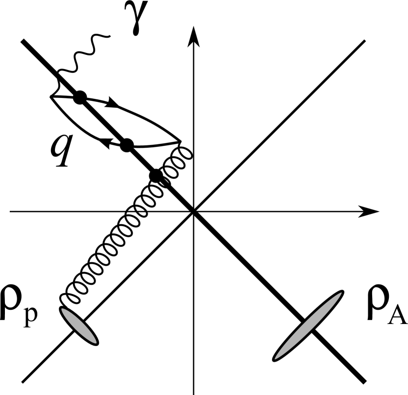
(d)

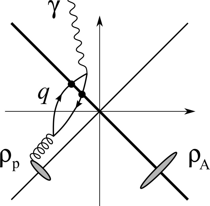
Figure 3: The connected $O(\rho_{p}^{1})$ contributions to the amplitude $\mathcal{M}_{\lambda}(\boldsymbol{k})$ corresponding to the decomposition in Eq. (21).

Next, we focus on the third (connected) $O(\rho_{p}^{1})$ contribution. It is convenient to decompose the amplitude using Eq. (9) for $S_{(0)}(x,y)$, which leads to

$$\begin{split}\mathcal{M}_{\lambda}(\boldsymbol{k})&=eg\int d^{4}x\,d^{4}y\,e^{ik\cdot x}\,\text{Tr}\bigl{[}\hbox to0.0pt{\hbox to5.00002pt{\hfil$\epsilon$\hfil}\hss}/_{\lambda}(\boldsymbol{k})S_{(0<<)}(x,y)\hbox to0.0pt{\hbox to7.50002pt{\hfil/\hfil}\hss}\mathcal{A}_{(1<)}(y)S_{(0<<)}(y,x)\bigr{]}\\ &+eg\int d^{4}x\,d^{4}y\,e^{ik\cdot x}\,\text{Tr}\bigl{[}\hbox to0.0pt{\hbox to5.00002pt{\hfil$\epsilon$\hfil}\hss}/_{\lambda}(\boldsymbol{k})S_{(0>>)}(x,y)\hbox to0.0pt{\hbox to7.50002pt{\hfil/\hfil}\hss}\mathcal{A}_{(1>)}(y)S_{(0>>)}(y,x)\bigr{]}\\ &+eg\int d^{4}x\,d^{4}y\,e^{ik\cdot x}\,\text{Tr}\bigl{[}\hbox to0.0pt{\hbox to5.00002pt{\hfil$\epsilon$\hfil}\hss}/_{\lambda}(\boldsymbol{k})S_{(0<>)}(x,y)\hbox to0.0pt{\hbox to7.50002pt{\hfil/\hfil}\hss}\mathcal{A}_{(1>)}(y)S_{(0><)}(y,x)\bigr{]}\\ &+eg\int d^{4}x\,d^{4}y\,e^{ik\cdot x}\,\text{Tr}\bigl{[}\hbox to0.0pt{\hbox to5.00002pt{\hfil$\epsilon$\hfil}\hss}/_{\lambda}(\boldsymbol{k})S_{(0><)}(x,y)\hbox to0.0pt{\hbox to7.50002pt{\hfil/\hfil}\hss}\mathcal{A}_{(1<)}(y)S_{(0<>)}(y,x)\bigr{]}\;.\end{split}$$ (21)

We depict the graphical representation of these individual contributions in Fig. 3. In the first (a) term the quark-antiquark pair is created by the gluon from $\rho_{p}$ and annihilated to a photon without crossing $\rho_{A}$. In the second (b) and the third (c) terms the gluon crosses $\rho_{A}$ and then produces a quark-antiquark pair. The created pair subsequently annihilates to a photon in the second term, but in the third term the pair first crosses $\rho_{A}$ back before annihilation. In the fourth (d) term the pair is created prior to the interaction with $\rho_{A}$ and after the created pair crosses $\rho_{A}$ it annihilates to a photon.

We now explain in details how the first three contributions in Eq. (21) vanish. Using Eq. (16) we can write the contribution (a) as

$$\int d^{4}x\,d^{4}y\,\theta(-x^{+})\theta(-y^{+})\,e^{ik\cdot x}\,\text{Tr}\bigl{[}\hbox to0.0pt{\hbox to5.00002pt{\hfil$\epsilon$\hfil}\hss}/_{\lambda}(\boldsymbol{k})S_{F}(x-y)\hbox to0.0pt{\hbox to7.50002pt{\hfil/\hfil}\hss}\mathcal{A}_{(1<)}(y)S_{F}(y-x)\bigr{]}\;.$$ (22)

In the region $x^{+},y^{+}<0$ the gluon field cannot develop a singlet component. The first contribution is then zero simply because of the color trace $\text{Tr}(T_{F}^{a})=0$. For the second component (b) with $x^{+},y^{+}>0$, because the CGC field is localized in $x^{+}$ as in Eq. (2), the quark loop part takes an identical structure as that of (a), and the quark loop picks up the color trace $\text{Tr}(T_{F}^{a})=0$. It is quite straightforward to confirm that the third component (c) is vanishing from the complex pole structures. We can intuitively understand this from the directions of particle and anti-particle flows in the light-cone coordinates as mentioned around Eq. (17): a positive energy should always flow from smaller to larger $x^{+}$. We also make a remark that (c) is clearly zero just because the quark-pair creation and annihilation points are not causally connected.

Thus, the only remaining contribution appears from the fourth term in Fig. 3 (d). Transforming the integrand in momentum space we can write the total $O(\rho_{p}^{1})$ amplitude as follows:

$$\mathcal{M}_{\lambda}(\boldsymbol{k}) =eg\int\frac{d^{4}p}{(2\pi)^{4}}\frac{d^{4}p^{\prime}}{(2\pi)^{4}}\frac{d^{4}q}{(2\pi)^{4}}(2\pi)\delta(p^{\prime+})(2\pi)\delta(p^{+}+p^{\prime+}-k^{+})$$

$$\quad\times\theta(q^{+})\theta(k^{+}-q^{+})\text{Tr}_{c}\bigl{[}U(\boldsymbol{p}_{\perp}^{\prime})\mathcal{A}_{(1<)}^{\mu}(p)U^{\dagger}(\boldsymbol{p}_{\perp}+\boldsymbol{p}_{\perp}^{\prime}-\boldsymbol{k}_{\perp})\bigr{]}$$

$$\quad\times\text{Tr}_{D}\bigl{[}\hbox to0.0pt{\hbox to5.00002pt{\hfil$\epsilon$\hfil}\hss}/_{\lambda}(\boldsymbol{k})S_{F}(q)\hbox to0.0pt{\hbox to6.00235pt{\hfil/\hfil}\hss}nS_{F}(q-p^{\prime})\gamma_{\mu}S_{F}(q-p-p^{\prime})\hbox to0.0pt{\hbox to6.00235pt{\hfil/\hfil}\hss}nS_{F}(q-k)\bigr{]}\;.$$ (23)

In the physical language, $q$ is the momentum running over the quark loop, $p$ is the momentum carried by the gluon field attached with $\rho_{p}$, $p^{\prime}$ and $p+p^{\prime}-k$ are the momenta inserted by the interaction with the CGC gluon field from $\rho_{A}$. We note that the $\theta$-functions are to keep the correct energy (longitudinal momentum) flows. Because the CGC fields convey only the transverse momenta, the integrals with respect to $p^{+}$ and $p^{\prime+}$ are trivially constrained by the $\delta$-functions. The integrals over $p^{-}$, $p^{\prime-}$ and $q^{-}$ are computed as we explain below. Taking into account the gluon field $\mathcal{A}_{(1<)}^{\mu}(p)$ as given in Eq. (4), we see that the integral over $p^{-}$ has two singularities; one above and the other below the real axis. We shall perform the $p^{-}$-integration by picking up the singularity in $S_{F}(q-p-p^{\prime})$ at

$$p^{-}=q^{-}-p^{\prime-}-\frac{\omega_{q-p-p^{\prime}}^{2}}{2(q^{+}-k^{+})}-i\epsilon\;.$$ (24)

Here we introduced a notation for the transverse energy as $\omega_{p}^{2}\equiv p_{\perp}^{2}+m^{2}$. Next, we calculate the integration over $p^{\prime-}$. Also in this case we find two singularities above and below the real axis. We pick up the singularity in $S_{F}(q-p^{\prime})$ at

$$p^{\prime-}=q^{-}-\frac{\omega_{q-p^{\prime}}^{2}}{2q^{+}}+i\epsilon\;.$$ (25)

The gluon fields $\mathcal{A}_{(1<)}^{\mu}$ in Eq. (4) have non-vanishing transverse components. Plugging Eqs. (24) and (25) into Eq. (4) we have $\mathcal{A}^{i}_{(1<)}(p)$ in the following form,

$$\mathcal{A}^{i}_{(1<)}(p)=ig\frac{1}{(k^{+}+i\epsilon)\Bigl{(}\frac{\omega_{q-p^{\prime}}^{2}}{2q^{+}}-\frac{\omega_{q-p-p^{\prime}}^{2}}{2(q^{+}-k^{+})}-i\epsilon\Bigr{)}}\,\frac{p^{i}}{p_{\perp}^{2}}\,\rho_{p}(\boldsymbol{p}_{\perp})\;,$$ (26)

where the $q^{-}$ dependence has canceled out. Therefore, for the $q^{-}$-integration there are two remaining singularities; one above the real axis from $S_{F}(q-k)$ and the other below the real axis from $S_{F}(q)$. We choose to pick up the singularity in $S_{F}(q)$ at

$$q^{-}=\frac{\omega^{2}_{q}}{2q^{+}}-i\epsilon\;.$$ (27)

Now, we still have the $q^{+}$-integration and three transverse integrations with respect to $\boldsymbol{p}_{\perp}$, $\boldsymbol{p}_{\perp}^{\prime}$, and $\boldsymbol{q}_{\perp}$. The amplitude has two non-trivial denominators coming from $\mathcal{A}^{i}_{(1<)}(p)$ and $S_{F}(q-k)$. We can further simplify the singular denominator as

$$\begin{split}&\biggl{[}\frac{\omega_{q-p^{\prime}}^{2}}{2q^{+}}-\frac{\omega_{q-p-p^{\prime}}^{2}}{2(q^{+}-k^{+})}\biggr{]}\biggl{[}2(q^{+}-k^{+})\biggl{(}\frac{\omega_{q}^{2}}{2q^{+}}-k^{-}\biggr{)}-\omega_{q-k}^{2}\biggr{]}\\ &=\frac{k^{+2}}{2q^{+2}(q^{+}-k^{+})}\bigl{[}(x\boldsymbol{k}_{\perp}-\boldsymbol{q}_{\perp})^{2}+m^{2}\bigr{]}\bigl{[}(x\boldsymbol{p}_{\perp}-\boldsymbol{q}_{\perp}+\boldsymbol{p}_{\perp}^{\prime})^{2}+m_{p}^{2}(x)\bigr{]}\;,\end{split}$$ (28)

where $x\equiv q^{+}/k^{+}$. Later we will use $x$ as an integration variable instead of $q^{+}$. In the above we defined $m_{p}^{2}(x)\equiv m^{2}+b(x)p_{\perp}^{2}$ with $b(x)\equiv x(1-x)$.

Let us turn to the calculation of the numerator. We have computed the Dirac trace with the help of FeynCalc [24]. Using the explicit form of the polarization vector,

$$\epsilon_{\lambda\mu}(\boldsymbol{k})=g_{\lambda\mu}-\frac{n_{\lambda}k_{\mu}+n_{\mu}k_{\lambda}}{n\cdot k}$$ (29)

with the physical polarizations $\lambda=1,2$, we find that the Dirac trace eventually leads to

$$\begin{split}&\text{Tr}_{D}\bigl{[}\hbox to0.0pt{\hbox to5.00002pt{\hfil$\epsilon$\hfil}\hss}/_{\lambda}(\boldsymbol{k})(\hbox to0.0pt{\hbox to5.00002pt{\hfil$q$\hfil}\hss}/+m)\hbox to0.0pt{\hbox to6.00235pt{\hfil/\hfil}\hss}n(\hbox to0.0pt{\hbox to5.00002pt{\hfil$q$\hfil}\hss}/-\hbox to0.0pt{\hbox to5.03125pt{\hfil/\hfil}\hss}p^{\prime}+m)\boldsymbol{p}_{\perp}\cdot\boldsymbol{\gamma}_{\perp}(\hbox to0.0pt{\hbox to5.00002pt{\hfil$q$\hfil}\hss}/-\hbox to0.0pt{\hbox to5.03125pt{\hfil/\hfil}\hss}p-\hbox to0.0pt{\hbox to5.03125pt{\hfil/\hfil}\hss}p^{\prime}+m)\hbox to0.0pt{\hbox to6.00235pt{\hfil/\hfil}\hss}n(\hbox to0.0pt{\hbox to5.00002pt{\hfil$q$\hfil}\hss}/-\hbox to0.0pt{\hbox to5.52084pt{\hfil/\hfil}\hss}k+m)\bigr{]}\\ &=8k^{+2}\bigl{[}R_{1}(\boldsymbol{p}_{\perp},\boldsymbol{p}_{\perp}^{\prime},\boldsymbol{q}_{\perp})(xk_{\lambda}-q_{\lambda})\\ &\qquad\qquad+R_{2}(\boldsymbol{k}_{\perp},\boldsymbol{p}_{\perp},\boldsymbol{q}_{\perp})(xp_{\lambda}-q_{\lambda}+p^{\prime}_{\lambda})+R_{3}(\boldsymbol{k}_{\perp},\boldsymbol{p}_{\perp},\boldsymbol{q}_{\perp})p_{\lambda}\bigr{]}~{},\end{split}$$ (30)

where we defined,

$$\begin{split}R_{1}(\boldsymbol{p}_{\perp},\boldsymbol{p}_{\perp}^{\prime},\boldsymbol{q}_{\perp})&\equiv a(x)b(x)\boldsymbol{p}_{\perp}^{2}-[1-4b(x)](x\boldsymbol{p}_{\perp}-\boldsymbol{q}_{\perp}+\boldsymbol{p}_{\perp}^{\prime})\cdot\boldsymbol{p}_{\perp}\;,\\ R_{2}(\boldsymbol{k}_{\perp},\boldsymbol{p}_{\perp},\boldsymbol{q}_{\perp})&\equiv(x\boldsymbol{k}_{\perp}-\boldsymbol{q}_{\perp})\cdot\boldsymbol{p}_{\perp}\;,\\ R_{3}(\boldsymbol{k}_{\perp},\boldsymbol{p}_{\perp},\boldsymbol{q}_{\perp})&\equiv(x\boldsymbol{k}_{\perp}-\boldsymbol{q}_{\perp})\cdot\boldsymbol{p}_{\perp}-m^{2}\;,\end{split}$$ (31)

and $a(x)\equiv x-\frac{1}{2}$, and see below Eq. (28) for the definition of $b(x)$. Finally, we put all the terms together to rewrite the amplitude as

$$\mathcal{M}_{\lambda}(\boldsymbol{k}) =\frac{eg^{2}}{\pi}\int_{0}^{1}dx\int\frac{d^{2}\boldsymbol{p}_{\perp}}{(2\pi)^{2}}\frac{d^{2}\boldsymbol{p}_{\perp}^{\prime}}{(2\pi)^{2}}\frac{d^{2}\boldsymbol{q}_{\perp}}{(2\pi)^{2}}\,\frac{1}{p_{\perp}^{2}}\,\frac{1}{(x\boldsymbol{k}_{\perp}-\boldsymbol{q}_{\perp})^{2}+m^{2}}$$

$$\qquad\times\frac{1}{(x\boldsymbol{p}_{\perp}-\boldsymbol{q}_{\perp}+\boldsymbol{p}_{\perp}^{\prime})^{2}+m_{p}^{2}(x)}\Bigl{\{}R_{1}(\boldsymbol{p}_{\perp},\boldsymbol{p}_{\perp}^{\prime},\boldsymbol{q}_{\perp})(xk_{\lambda}-q_{\lambda})$$

$$\quad+R_{2}(\boldsymbol{k}_{\perp},\boldsymbol{p}_{\perp},\boldsymbol{q}_{\perp})(xp_{\lambda}-q_{\lambda}+p_{\lambda}^{\prime})+R_{3}(\boldsymbol{k}_{\perp},\boldsymbol{p}_{\perp},\boldsymbol{q}_{\perp})p_{\lambda}\Bigr{\}}$$

$$\qquad\times\text{Tr}_{c}\bigl{[}U(\boldsymbol{p}_{\perp}^{\prime})\,\rho_{p}(\boldsymbol{p}_{\perp})\,U^{\dagger}(\boldsymbol{p}_{\perp}+\boldsymbol{p}_{\perp}^{\prime}-\boldsymbol{k}_{\perp})\bigr{]}\;.$$ (32)

We now make a few general comments about the above amplitude. First, decomposing the amplitude as $\mathcal{M}_{\lambda}(\boldsymbol{k})=\epsilon^{\mu}_{\lambda}(\boldsymbol{k})\mathcal{T}_{\mu}(\boldsymbol{k})$, we have explicitly checked that the Ward identity, $k_{\mu}\mathcal{T}^{\mu}(\boldsymbol{k})=0$, holds. The relevant steps of this calculation are summarized in A. Second, we note that the numerator depends on a combination of $x\boldsymbol{k}_{\perp}-\boldsymbol{q}_{\perp}$ and the same dependence is found in the denominator. This leads to a consequence that any collinear singularity in the $\boldsymbol{q}_{\perp}$-integration even at $m=0$ does not appear due to the cancellation by the numerator.

At this point it is useful to replace the integration variable as $\boldsymbol{p}_{\perp}^{\prime}\to\boldsymbol{l}_{\perp}\equiv\boldsymbol{p}_{\perp}^{\prime}-\boldsymbol{q}_{\perp}+\frac{1}{2}\boldsymbol{p}_{\perp}$. We transform the Wilson lines back in position space for convenience. Shifting the integration variables as $x\boldsymbol{k}_{\perp}-\boldsymbol{q}_{\perp}\to\boldsymbol{q}_{\perp}$ and $a(x)\boldsymbol{p}_{\perp}+\boldsymbol{l}_{\perp}\to\boldsymbol{l}_{\perp}$, we can evaluate the transverse momentum integrals with the help of

$$\begin{split}\int\frac{d^{2}q_{\perp}}{(2\pi)^{2}}\,\frac{e^{i\boldsymbol{q}_{\perp}\cdot\boldsymbol{x}_{\perp}}}{q_{\perp}^{2}+m^{2}}&=\frac{1}{2\pi}K_{0}(x_{\perp}m)\;,\\ \int\frac{d^{2}q_{\perp}}{(2\pi)^{2}}\,\frac{e^{i\boldsymbol{q}_{\perp}\cdot\boldsymbol{x}_{\perp}}}{q_{\perp}^{2}+m^{2}}\,\boldsymbol{q}_{\perp}\cdot\boldsymbol{y}_{\perp}&=\frac{i}{2\pi}\,\hat{\boldsymbol{x}}_{\perp}\cdot\boldsymbol{y}_{\perp}\,mK_{1}(x_{\perp}m)\;,\end{split}$$ (33)

where $\hat{\boldsymbol{x}}_{\perp}\equiv\boldsymbol{x}_{\perp}/x_{\perp}$ and $K_{0,1}(x)$ are the modified Bessel functions of the zeroth and the first order, respectively. After all, the final expression for the amplitude that we will use for the computation of the photon production rate is

$$\mathcal{M}_{\lambda}(\boldsymbol{k}) =\frac{eg^{2}}{4\pi^{3}}\int_{0}^{1}dx\int d^{2}\boldsymbol{u}_{\perp}\,d^{2}\boldsymbol{v}_{\perp}\int\frac{d^{2}\boldsymbol{p}_{\perp}}{(2\pi)^{2}}\,e^{-i(\boldsymbol{k}_{\perp}-\boldsymbol{p}_{\perp})\cdot[\boldsymbol{v}_{\perp}+a(x)\boldsymbol{u}_{\perp}]}$$

$$\quad\times\frac{\rho_{p}^{a}(\boldsymbol{p}_{\perp})}{p_{\perp}^{2}}\,\text{Tr}_{c}\biggl{[}U\Bigl{(}\boldsymbol{v}_{\perp}+\frac{\boldsymbol{u}_{\perp}}{2}\Bigr{)}T_{F}^{a}U^{\dagger}\Bigl{(}\boldsymbol{v}_{\perp}-\frac{\boldsymbol{u}_{\perp}}{2}\Bigr{)}\biggr{]}$$

$$\quad\times\bigl{[}\hat{u}_{\lambda}p_{\perp}\Psi_{1}(\boldsymbol{p}_{\perp},\boldsymbol{u}_{\perp},x)+p_{\lambda}\Psi_{2}(\boldsymbol{p}_{\perp},\boldsymbol{u}_{\perp},x)\bigr{]}\;,$$ (34)

where

$$\Psi_{1}(\boldsymbol{p}_{\perp},\boldsymbol{u}_{\perp},x) \equiv-4ia(x)b(x)p_{\perp}K_{0}(m_{p}(x)u_{\perp})mK_{1}(mu_{\perp})$$

$$\quad+4b(x)\hat{\boldsymbol{p}}_{\perp}\cdot\hat{\boldsymbol{u}}_{\perp}m_{p}(x)K_{1}(m_{p}(x)u_{\perp})mK_{1}(mu_{\perp})\;,$$ (35)

$$\Psi_{2}(\boldsymbol{p}_{\perp},\boldsymbol{u}_{\perp},x) \equiv mK_{1}(mu_{\perp})m_{p}(x)K_{1}(m_{p}(x)u_{\perp})$$

$$\quad+m^{2}K_{0}(mu_{\perp})K_{0}(m_{p}(x)u_{\perp})\;.$$ (36)

These functions $\Psi_{1}$ and $\Psi_{2}$, have the following symmetry properties:

$$\begin{split}\Psi_{i}(\boldsymbol{p}_{\perp},\boldsymbol{u}_{\perp},x)&=\Psi_{i}^{*}(\boldsymbol{p}_{\perp},-\boldsymbol{u}_{\perp},x);,\\ \Psi_{i}(\boldsymbol{p}_{\perp},\boldsymbol{u}_{\perp},x)&=\Psi_{i}^{*}(\boldsymbol{p}_{\perp},\boldsymbol{u}_{\perp},1-x)\;,\\ \Psi_{i}(\boldsymbol{p}_{\perp},\boldsymbol{u}_{\perp},x)&=(-1)^{i}\Psi_{i}(\boldsymbol{p}_{\perp},-\boldsymbol{u}_{\perp},1-x)\;.\end{split}$$ (37)

It should be noted that the Wilson lines take care of resummation over multiple gluon scatterings and we can recover the naive diagrammatic perturbation theory by expanding the Wilson lines in the number of the gluon fields. The contribution with a single gluon (i.e. no gluon from the Wilson lines) vanishes because of the color trace. The contribution with two gluons vanishes because of charge conjugation or Furry’s theorem. The lowest non-vanishing diagram should involve three gluons, namely, one from $\rho_{p}$ and two from $\rho_{A}$, and an emitted photon. It is important to realize that this contribution is UV finite due to gauge invariance. That is, if a three-gluon and one-photon operator came from a UV divergent loop, it would have to correspond to a dimension four operator, but there is no such gauge invariant operator with dimension four involving three gluons and one photon. Because higher-order contributions are more UV suppressed, our resummed result in Eq. (34) is completely UV finite.

4 Photon production rate

Squaring the amplitude we obtain the probability density for the emission of a single photon. This expression explicitly depends on the color sources, $\rho_{p}$ and $\rho_{A}$, and we should take a color average over the color sources in the proton and in the nucleus. To get the minimum biased photon production rate we integrate over the impact parameters $\boldsymbol{b}$. In total, the photon production rate, that is, the number of photons produced per unit $\boldsymbol{k}_{\perp}$ and per unit rapidity $y\equiv\frac{1}{2}\ln(k^{+}/k^{-})$ is given as

$$dN=\frac{d^{3}\boldsymbol{k}}{(2\pi)^{3}(2k^{0})}\int d^{2}\boldsymbol{b}\,\bigl{\langle}\mathcal{M}_{\lambda}(\boldsymbol{k})\mathcal{M}_{\lambda}^{\ast}(\boldsymbol{k})\bigr{\rangle}=\frac{d^{2}\boldsymbol{k}_{\perp}dy}{16\pi^{3}}\int d^{2}\boldsymbol{b}\,\bigl{\langle}\mathcal{M}_{\lambda}(\boldsymbol{k})\mathcal{M}_{\lambda}^{\ast}(\boldsymbol{k})\bigr{\rangle}\;,$$ (38)

where a summation over $\lambda$ is implied. With $\langle\cdots\rangle$ we denoted taking the color average, that is defined for a general operator $\mathcal{O}[\rho_{p},\rho_{A}]$ as

$$\bigl{\langle}\mathcal{O}[\rho_{p},\rho_{A}]\bigr{\rangle}=\int[d\rho_{p}][d\rho_{A}]W_{p}[x_{p};\rho_{p}]W_{A}[x_{A};\rho_{A}]\mathcal{O}[\rho_{p},\rho_{A}]\;,$$ (39)

where the functionals, $W_{p,A}[x_{p,A};\rho_{p,A}]$, incorporate the small-$x$ evolution of the proton and the nucleus wave-functions. The non-linear evolution of $W_{p,A}[x_{p,A};\rho_{p,A}]$ is governed by the Balitsky-Jalilian–Marian-Iancu-McLerran-Leonidov-Kovner (B-JIMWLK) equation [28, 29], and we will later adopt a Gaussian approximated solution for numerical calculations.

4.1 Squaring the amplitude

For variables in the complex conjugated amplitude, we will use primes on the coordinates $\boldsymbol{u}_{\perp}$, $\boldsymbol{v}_{\perp}$, the gluon momentum $\boldsymbol{p}_{\perp}$, the momentum fraction $x$, and the color index $a$, which all characterize the amplitude (34). For the color average over $\rho_{p}$ we follow the notation of Ref. [18] to define the unintegrated gluon distribution function as

$$g^{2}\bigl{\langle}\rho_{p}^{a}(\boldsymbol{p}_{\perp})\rho_{p}^{{\dagger}a^{\prime}}(\boldsymbol{p}_{\perp})\bigr{\rangle}\equiv\frac{\delta^{aa^{\prime}}}{\pi(N_{c}^{2}-1)}p_{\perp}^{2}\,\varphi_{p}(p_{\perp})\;,$$ (40)

where the color average is taken for the proton. Transverse momentum integral over $\varphi_{p}(p_{\perp})$ will be proportional $n_{g}$ that we discussed in Sec. 2 (see Eq. (57) for a precise relation). The photon production rate is also proportional to the Wilson line product, and we define,

$$S(\boldsymbol{y}_{\perp},\boldsymbol{z}_{\perp},\boldsymbol{y}_{\perp}^{\prime},\boldsymbol{z}_{\perp}^{\prime})\equiv\frac{1}{N_{c}}\Bigl{\langle}\text{Tr}_{c}\bigl{[}U(\boldsymbol{y}_{\perp})T_{F}^{a}U^{\dagger}(\boldsymbol{z}_{\perp})\bigr{]}\text{Tr}_{c}\bigl{[}U(\boldsymbol{z}_{\perp}^{\prime})T_{F}^{a}U^{\dagger}(\boldsymbol{y}_{\perp}^{\prime})\bigr{]}\Bigr{\rangle}\;,$$ (41)

where the color average is taken for the nucleus. We have the original coordinate variables through $\boldsymbol{y}_{\perp}=\boldsymbol{v}_{\perp}-\boldsymbol{u}_{\perp}/2$, $\boldsymbol{z}_{\perp}=\boldsymbol{v}_{\perp}+\boldsymbol{u}_{\perp}/2$ and $\boldsymbol{y}_{\perp}^{\prime}=\boldsymbol{v}_{\perp}^{\prime}-\boldsymbol{u}_{\perp}^{\prime}/2$, and $\boldsymbol{z}_{\perp}^{\prime}=\boldsymbol{v}_{\perp}^{\prime}+\boldsymbol{u}_{\perp}^{\prime}/2$. Next, we shift the coordinates of the proton position as $\boldsymbol{v}_{\perp}\to\boldsymbol{v}_{\perp}-\boldsymbol{b}$ and $\boldsymbol{v}_{\perp}^{\prime}\to\boldsymbol{v}_{\perp}^{\prime}-\boldsymbol{b}$. In this way we moved the origin of the coordinate system from the proton to the nucleus. In the infinite limit of nucleus transverse size the correlator (41) is invariant under translation in the transverse plane and therefore independent of $\boldsymbol{b}$. The integration over the impact parameter thereby results in a factor,

$$\int d^{2}\boldsymbol{b}\,e^{-i(\boldsymbol{p}_{\perp}-\boldsymbol{p}_{\perp}^{\prime})\cdot\boldsymbol{b}}=(2\pi)^{2}\delta^{(2)}(\boldsymbol{p}_{\perp}-\boldsymbol{p}_{\perp}^{\prime})\;.$$ (42)

As a further consequence from translational invariance, the correlator (41) is independent of the overall center of mass coordinate, $\boldsymbol{v}_{\perp}+\boldsymbol{v}_{\perp}^{\prime}$, so that the integration over $\boldsymbol{v}_{\perp}$ and $\boldsymbol{v}_{\perp}^{\prime}$ is reduced to

$$\int d^{2}\boldsymbol{v}_{\perp}d^{2}\boldsymbol{v}_{\perp}^{\prime}=\pi R_{A}^{2}\int d^{2}\boldsymbol{w}_{\perp}\;,$$ (43)

where $\pi R_{A}^{2}$ is the transverse area of the nuclei and $\boldsymbol{w}_{\perp}\equiv\boldsymbol{v}_{\perp}-\boldsymbol{v}_{\perp}^{\prime}$.

For a given polarization $\lambda$, the amplitude (34) is a linear combination of $\hat{u}_{\lambda}$ and $p_{\lambda}$. Squaring the amplitude and summing over $\lambda$ results in four terms proportional to $\Psi_{1}\Psi^{\prime\ast}_{1}\,\hat{\boldsymbol{u}}_{\perp}\!\!\cdot\hat{\boldsymbol{u}}_{\perp}^{\prime}$, $\Psi_{2}\Psi^{\prime\ast}_{2}$, $\Psi_{1}\Psi^{\prime\ast}_{2}\,\hat{\boldsymbol{u}}_{\perp}\!\!\cdot\hat{\boldsymbol{p}}_{\perp}$, and $\Psi_{2}\Psi^{\prime\ast}_{1}\,\hat{\boldsymbol{p}}_{\perp}\!\!\cdot\hat{\boldsymbol{u}}_{\perp}^{\prime}$, respectively. Here we used an abbreviated notation $\Psi_{1,2}\equiv\Psi_{1,2}(\boldsymbol{p}_{\perp},\boldsymbol{u}_{\perp},x)$ and $\Psi^{\prime}_{1,2}\equiv\Psi_{1,2}(\boldsymbol{p}_{\perp}^{\prime},\boldsymbol{u}_{\perp}^{\prime},x^{\prime})$. The last two terms are shown to be equal by exchanging the original and the primed coordinates and momentum fractions, that is, $\boldsymbol{u}_{\perp}\leftrightarrow\boldsymbol{u}_{\perp}^{\prime}$, $x\leftrightarrow x^{\prime}$, followed by a reflection $\boldsymbol{u}_{\perp}\to-\boldsymbol{u}_{\perp}$ and $\boldsymbol{u}_{\perp}^{\prime}\to-\boldsymbol{u}_{\perp}^{\prime}$. Such a transformation leaves the exponential factor $e^{-i(\boldsymbol{k}_{\perp}-\boldsymbol{p}_{\perp})\cdot[\boldsymbol{v}_{\perp}-\boldsymbol{v}_{\perp}^{\prime}+a(x)\boldsymbol{u}_{\perp}-a(x^{\prime})\boldsymbol{u}_{\perp}^{\prime}]}$ as well as the Wilson line product (41) intact. Due to the relations (37), we can write $\Psi_{1}\Psi^{\prime*}_{2}\,\hat{\boldsymbol{u}}_{\perp}\cdot\hat{\boldsymbol{p}}_{\perp}=\Psi_{2}\Psi^{\prime*}_{1}\,\hat{\boldsymbol{p}}_{\perp}\cdot\hat{\boldsymbol{u}}_{\perp}^{\prime}$, under the integral.

Finally, the expression for the photon production rate takes the form of

$$\begin{split}&\frac{1}{\pi R_{A}^{2}}\frac{dN}{d^{2}\boldsymbol{k}_{\perp}dy}=\frac{\alpha\,\alpha_{s}}{16\pi^{8}}\frac{N_{c}}{N_{c}^{2}-1}\int_{0}^{1}dx\,dx^{\prime}\int d^{2}\boldsymbol{u}_{\perp}\,d^{2}\boldsymbol{u}_{\perp}^{\prime}\,d^{2}\boldsymbol{w}_{\perp}\,e^{-i\boldsymbol{k}_{\perp}\cdot\boldsymbol{r}_{\perp}}\\ &\quad\times S\Bigl{(}\boldsymbol{u}_{\perp}-\frac{\boldsymbol{v}_{\perp}}{2},\boldsymbol{u}_{\perp}+\frac{\boldsymbol{v}_{\perp}}{2},\boldsymbol{u}_{\perp}^{\prime}-\frac{\boldsymbol{v}_{\perp}^{\prime}}{2},\boldsymbol{u}_{\perp}^{\prime}+\frac{\boldsymbol{v}_{\perp}^{\prime}}{2}\Bigr{)}\\ &\quad\times\int\frac{d^{2}\boldsymbol{p}_{\perp}}{(2\pi)^{2}}\frac{p_{\perp}^{4}\varphi_{p}(p_{\perp})}{(p_{\perp}^{2}+\Lambda_{\rm QCD}^{2})^{2}}\,e^{i\boldsymbol{p}_{\perp}\cdot\boldsymbol{r}_{\perp}}\bigl{(}\hat{\boldsymbol{u}}_{\perp}\!\!\cdot\hat{\boldsymbol{u}}_{\perp}^{\prime}\Psi_{1}\Psi^{\prime\ast}_{1}+\Psi_{2}\Psi^{\prime\ast}_{2}+2\hat{\boldsymbol{u}}_{\perp}\!\!\cdot\hat{\boldsymbol{p}}_{\perp}\Psi_{1}\Psi^{\prime\ast}_{2}\bigr{)}\;,\end{split}$$ (44)

where we regulate the infrared divergence from massless gluons by an infrared cutoff $\Lambda_{\rm QCD}$ and we introduced a notation, $\boldsymbol{r}_{\perp}\equiv\boldsymbol{w}_{\perp}+a(x)\boldsymbol{u}_{\perp}-a(x^{\prime})\boldsymbol{u}_{\perp}^{\prime}$. We see that Eq. (44) is $\mathcal{O}(\alpha\,\alpha_{s}\,n_{g})$ and this expression represents one of the main results in this work.

4.2 Taking the color average

Applying the Fierz transformation to the correlator (41) we find,

$$\begin{split}S(\boldsymbol{y}_{\perp},\boldsymbol{z}_{\perp},\boldsymbol{y}_{\perp}^{\prime},\boldsymbol{z}_{\perp}^{\prime})&=\frac{1}{2}\Bigl{[}Q(\boldsymbol{y}_{\perp},\boldsymbol{z}_{\perp},\boldsymbol{y}_{\perp}^{\prime},\boldsymbol{z}_{\perp}^{\prime})\\ &\quad-\frac{1}{N_{c}^{2}}\big{\langle}\text{Tr}_{c}[U(\boldsymbol{y}_{\perp})U^{\dagger}(\boldsymbol{z}_{\perp})]\text{Tr}_{c}[U(\boldsymbol{y}_{\perp}^{\prime})U^{\dagger}(\boldsymbol{z}_{\perp}^{\prime})]\big{\rangle}\Bigr{]}\;,\end{split}$$ (45)

where

$$Q(\boldsymbol{y}_{\perp},\boldsymbol{z}_{\perp},\boldsymbol{y}_{\perp}^{\prime},\boldsymbol{z}_{\perp}^{\prime})\equiv\frac{1}{N_{c}}\bigl{\langle}\text{Tr}_{c}[U(\boldsymbol{y}_{\perp})U^{\dagger}(\boldsymbol{z}_{\perp}^{\prime})U(\boldsymbol{y}_{\perp}^{\prime})U^{\dagger}(\boldsymbol{z}_{\perp})]\bigr{\rangle}\;,$$ (46)

is the color average over the quadrupole operator. The second term in the large $N_{c}$ limit and for large nuclei becomes the product of the dipole operators as

$$\frac{1}{N_{c}^{2}}\bigl{\langle}\text{Tr}_{c}[U(\boldsymbol{y}_{\perp})U^{\dagger}(\boldsymbol{z}_{\perp})]\text{Tr}_{c}[U(\boldsymbol{y}_{\perp}^{\prime})U^{\dagger}(\boldsymbol{z}_{\perp}^{\prime})]\bigr{\rangle}\to D(\boldsymbol{y}_{\perp},\boldsymbol{z}_{\perp})\,D(\boldsymbol{z}_{\perp}^{\prime},\boldsymbol{y}_{\perp}^{\prime})\;,$$ (47)

and the color average over the dipole operator is given as

$$D(\boldsymbol{y}_{\perp},\boldsymbol{z}_{\perp})\equiv\frac{1}{N_{c}}\bigl{\langle}\text{Tr}_{c}[U(\boldsymbol{y}_{\perp})U^{\dagger}(\boldsymbol{z}_{\perp})]\bigr{\rangle}\;.$$ (48)

The expression (45) coincides with the so-called “inelastic quadrupole” [25] (see also Refs. [26, 27] for phenomenological applications to gluon-gluon and quarkonium production, respectively.

The general frameworks for the small-$x$ evolution of the dipole and the quadrupole are incorporated in the B-JIMWLK equations [28, 29]. The dipole evolution is closed in the large $N_{c}$ limit where it is known as the Balitsky-Kovchegov (BK) equation [28, 22, 30]. Concerning the phenomenological applications, the running coupling BK (rcBK) equation [31] is widely used. However, for the quadrupole evolution such a simplification has not been found. So far, it has been considered only for some very specific configurations [32]. Eventually, one would want to constrain the quadrupole evolution by using experimental data as it is done for the rcBK evolution by the DIS data from HERA.

In this work, as a preliminary for going into such quantitative studies, we will make a Gaussian approximation for the color distribution over the nuclei $W_{A}[x_{A};\rho_{A}]$, which defines the McLerran-Venugopalan (MV) model [1] as

$$\bigl{\langle}\rho_{A}^{a}(\boldsymbol{x}_{\perp})\rho_{A}^{b}(\boldsymbol{y}_{\perp})\bigr{\rangle}=g^{2}\delta^{ab}\mu_{A}^{2}\delta^{(2)}(\boldsymbol{x}_{\perp}-\boldsymbol{y}_{\perp})\;,$$ (49)

where the parameter $\mu_{A}$ is related to the saturation momentum $Q_{s}$. Here we shall employ a simple definition of $Q_{s}$ by

$$Q_{s}^{2}\equiv\frac{N_{c}^{2}-1}{4N_{c}}g^{4}\mu_{A}^{2}\;.$$ (50)

The MV model for the nuclei takes into account the multiple scattering effect, and typically, the MV model is considered to work up to a moderate value of $x_{A}\sim 10^{-2}$. To reach a region with far smaller $x_{A}$ we should consider the MV model as an initial condition for the evolution equations.

Using the standard techniques of the MV model [18, 33, 34] we have found it most convenient to directly calculate $S(\boldsymbol{y}_{\perp},\boldsymbol{z}_{\perp},\boldsymbol{y}_{\perp}^{\prime},\boldsymbol{z}_{\perp}^{\prime})$ in position space. The calculation steps are collected in C leading to the following result:

$$\begin{split}S(\boldsymbol{y}_{\perp},\boldsymbol{z}_{\perp},\boldsymbol{y}_{\perp}^{\prime},\boldsymbol{z}_{\perp}^{\prime})&=\frac{1}{N_{c}}\frac{(N_{c}^{2}-1)(\beta-\alpha)}{\sqrt{N_{c}^{2}(\alpha-\gamma)^{2}-4(\alpha-\beta)(\beta-\gamma)}}\\ &\quad\times\exp\biggl{[}-\frac{2\beta+(N_{c}^{2}-2)(\alpha+\gamma)}{N_{c}^{2}-1}\biggr{]}\\ &\quad\times\sinh\biggl{[}\frac{N_{c}}{N_{c}^{2}-1}\sqrt{N_{c}^{2}(\alpha-\gamma)^{2}-4(\alpha-\beta)(\beta-\gamma)}\biggr{]}\;.\end{split}$$ (51)

We note that the above result does not rely on the large-$N_{c}$ limit. Here we defined functions, $\alpha$, $\beta$, and $\gamma$ as

$$\begin{split}&2\alpha(\boldsymbol{y}_{\perp},\boldsymbol{z}_{\perp},\boldsymbol{y}_{\perp}^{\prime},\boldsymbol{z}_{\perp}^{\prime})\equiv B_{2}(|\boldsymbol{y}_{\perp}-\boldsymbol{z}_{\perp}^{\prime}|)+B_{2}(|\boldsymbol{z}_{\perp}-\boldsymbol{y}_{\perp}^{\prime}|)\;,\\ &2\beta(\boldsymbol{y}_{\perp},\boldsymbol{z}_{\perp},\boldsymbol{y}_{\perp}^{\prime},\boldsymbol{z}_{\perp}^{\prime})\equiv B_{2}(|\boldsymbol{y}_{\perp}-\boldsymbol{y}_{\perp}^{\prime}|)+B_{2}(|\boldsymbol{z}_{\perp}-\boldsymbol{z}_{\perp}^{\prime}|)\;,\\ &2\gamma(\boldsymbol{y}_{\perp},\boldsymbol{z}_{\perp},\boldsymbol{y}_{\perp}^{\prime},\boldsymbol{z}_{\perp}^{\prime})\equiv B_{2}(|\boldsymbol{y}_{\perp}-\boldsymbol{z}_{\perp}|)+B_{2}(|\boldsymbol{y}_{\perp}^{\prime}-\boldsymbol{z}_{\perp}^{\prime}|)\;.\end{split}$$ (52)

with $B_{2}$ having the following explicit expression [33],

$$\begin{split}B_{2}(x_{\perp})&\equiv 2Q_{s}^{2}\int_{0}^{\infty}\frac{k_{\perp}dk_{\perp}}{2\pi}\,\frac{1-J_{0}(k_{\perp}x_{\perp})}{(k_{\perp}^{2}+\Lambda_{\rm QCD}^{2})^{2}}\\ &=\frac{1}{2\pi}\frac{Q_{s}^{2}}{\Lambda_{\rm QCD}^{2}}\Bigl{[}1-x_{\perp}\Lambda_{\rm QCD}K_{1}(x_{\perp}\Lambda_{\rm QCD})\Bigr{]}\;,\end{split}$$ (53)

where we use $\Lambda_{\rm QCD}$ as an infrared regulator again. It would be useful to point out that the above expression for $S$ has the following symmetries:

$$\begin{split}S(\boldsymbol{z}_{\perp},\boldsymbol{y}_{\perp},\boldsymbol{z}_{\perp}^{\prime},\boldsymbol{y}_{\perp}^{\prime})&=S(-\boldsymbol{y}_{\perp},-\boldsymbol{z}_{\perp},-\boldsymbol{y}_{\perp}^{\prime},-\boldsymbol{z}_{\perp}^{\prime})~{},\\ S(\boldsymbol{z}_{\perp},\boldsymbol{y}_{\perp},\boldsymbol{z}_{\perp}^{\prime},\boldsymbol{y}_{\perp}^{\prime})&=S(\boldsymbol{y}_{\perp},\boldsymbol{z}_{\perp},\boldsymbol{y}_{\perp}^{\prime},\boldsymbol{z}_{\perp}^{\prime})\;.\end{split}$$ (54)

Although we will not use it for our numerical calculations, we can check that the large-$N_{c}$ limit simplifies the results into

$$S(\boldsymbol{y}_{\perp},\boldsymbol{z}_{\perp},\boldsymbol{y}_{\perp}^{\prime},\boldsymbol{z}_{\perp}^{\prime})=\frac{\alpha-\beta}{2(\alpha-\gamma)}(e^{-2\alpha}-e^{-2\gamma})+\mathcal{O}(N_{c}^{-2})\;.$$ (55)

This large-$N_{c}$ expression coincides with the one found in Ref. [25]. Another useful check of Eq. (51) is that the photon rate involving two gluons vanishes. The expansion in the number of the gluon lines from the nucleus is equivalent to an expansion in powers of $Q_{s}^{2}$. Up to the order $\mathcal{O}(Q_{s}^{6})$ we get,

$$S(\boldsymbol{y}_{\perp},\boldsymbol{z}_{\perp},\boldsymbol{y}_{\perp}^{\prime},\boldsymbol{z}_{\perp}^{\prime})=-(\alpha-\beta)+\frac{N_{c}^{2}-2}{N_{c}^{2}-1}(\alpha-\beta)\biggl{(}\alpha+\gamma+\frac{2\beta}{N_{c}^{2}-2}\biggr{)}+\mathcal{O}(Q_{s}^{6})\;,$$ (56)

where the first term is $\mathcal{O}(Q_{s}^{2})$ and the second is $\mathcal{O}(Q_{s}^{4})$. It is easy to confirm that the $\mathcal{O}(Q_{s}^{2})$ term is odd under $\boldsymbol{u}_{\perp}\to-\boldsymbol{u}_{\perp}$ or $\boldsymbol{u}_{\perp}^{\prime}\to-\boldsymbol{u}_{\perp}^{\prime}$. This symmetry is not shared with the full expression (53). We can use this symmetry to demonstrate that the rate vanishes to this order. We split the integration over $x$ as $\int_{0}^{1}dx=\int_{0}^{1/2}dx+\int_{1/2}^{1}dx$ and in the second term we transform the variable as $x\to 1-x$. Transforming $\boldsymbol{u}_{\perp}\to-\boldsymbol{u}_{\perp}$ and using the last line of Eq. (37) we find $-\hat{\boldsymbol{u}}_{\perp}\Psi_{1}(\boldsymbol{p}_{\perp},-\boldsymbol{u}_{\perp},1-x)+\hat{\boldsymbol{p}}_{\perp}\Psi_{2}(\boldsymbol{p}_{\perp},-\boldsymbol{u}_{\perp},1-x)=\hat{\boldsymbol{u}}_{\perp}\Psi_{1}(\boldsymbol{p}_{\perp},\boldsymbol{u}_{\perp},x)+\hat{\boldsymbol{p}}_{\perp}\Psi_{2}(\boldsymbol{p}_{\perp},\boldsymbol{u}_{\perp},x)$. Since the first term in the expansion (56) is odd in $\boldsymbol{u}_{\perp}\to-\boldsymbol{u}_{\perp}$, two contributions from $\int_{0}^{1/2}dx$ and $\int_{1/2}^{1}dx$ cancel out and the $\mathcal{O}(Q_{s}^{2})$ order vanishes.

5 Numerical results

In the application to the pair $\bar{q}q$ production it was shown in Ref. [18] that the quadrupole correlator $Q(\boldsymbol{y}_{\perp},\boldsymbol{z}_{\perp},\boldsymbol{y}_{\perp}^{\prime},\boldsymbol{z}_{\perp}^{\prime})$ factorizes in the large-$N_{c}$ limit to a product of two dipoles, as mentioned before, and thus the large-$N_{c}$ limit greatly reduces the numerical cost in the evaluation of this process. For the inelastic quadrupole $S(\boldsymbol{y}_{\perp},\boldsymbol{z}_{\perp},\boldsymbol{y}_{\perp}^{\prime},\boldsymbol{z}_{\perp}^{\prime})$ found here for the annihilation photon production, there is a cancellation in the leading order in the large-$N_{c}$ limit between the first term and the second term in Eq. (45). As a consequence, the next order in the expansion of Eq. (55) does no longer factorize. A simultaneous numerical integration over the complete set of coordinates characterizing the inelastic quadrupole is necessary. In the numerical calculations below we use the form of the inelastic quadrupole (51) without any large-$N_{c}$ approximation. Then, we must specify the unintegrated gluon distribution inside the proton $\varphi_{p}(p_{\perp})$ appearing in the rate (44). We will use the MV model for the proton to fix $\varphi_{p}(p_{\perp})$ as

$$p_{\perp}^{2}\varphi_{p}(p_{\perp})=4\pi\,N_{c}n_{g}\,\pi R_{p}^{2}\;,$$ (57)

where $\pi R_{p}^{2}$ is the transverse area of the proton and $n_{g}$ is the transverse gluon density parameter with mass dimension 2.

5.1 Details of the numerical procedure

To explain the steps of the numerical calculation we introduce a notation for convenience. We replace the integration variable $\boldsymbol{w}_{\perp}$ with $\boldsymbol{r}_{\perp}$ as defined by $\boldsymbol{w}_{\perp}=\boldsymbol{r}_{\perp}-a(x)\boldsymbol{u}_{\perp}+a(x^{\prime})\boldsymbol{u}_{\perp}^{\prime}$. The benefit of this is that we can write the integration in the following form,

$$\frac{1}{\pi R_{A}^{2}\,\pi R_{p}^{2}\,\alpha_{s}n_{g}}\cdot\frac{dN}{d^{2}\boldsymbol{k}_{\perp}dy}=\frac{\alpha}{8\pi^{8}}\frac{N_{c}^{2}}{N_{c}^{2}-1}\int d^{2}\boldsymbol{r}_{\perp}\,e^{-i\boldsymbol{k}_{\perp}\cdot\boldsymbol{r}_{\perp}}F(r_{\perp})\;,$$ (58)

where we defined $F(r_{\perp})$ as

$$F(r_{\perp})\equiv\int_{0}^{1}dxdx^{\prime}\int d^{2}\boldsymbol{u}_{\perp}d^{2}\boldsymbol{u}_{\perp}^{\prime}\,f(x,x^{\prime},\boldsymbol{u}_{\perp},\boldsymbol{u}_{\perp}^{\prime},\boldsymbol{r}_{\perp})\;,$$ (59)

with

$$\begin{split}&f(x,x^{\prime},\boldsymbol{u}_{\perp},\boldsymbol{u}_{\perp}^{\prime},\boldsymbol{r}_{\perp})\equiv\tilde{S}(\boldsymbol{u}_{\perp},\boldsymbol{u}_{\perp}^{\prime},\boldsymbol{r}_{\perp}-a(x)\boldsymbol{u}_{\perp}+a(x^{\prime})\boldsymbol{u}_{\perp}^{\prime})\\ &\times\int\frac{d^{2}\boldsymbol{p}_{\perp}}{2\pi}\frac{p_{\perp}^{4}\,e^{i\boldsymbol{p}_{\perp}\cdot\boldsymbol{r}_{\perp}}}{(p_{\perp}^{2}+\Lambda_{\rm QCD}^{2})^{2}}\bigl{(}\hat{\boldsymbol{u}}_{\perp}\!\!\cdot\hat{\boldsymbol{u}}_{\perp}^{\prime}\Psi_{1}\Psi^{\prime\ast}_{1}+\Psi_{2}\Psi^{\prime\ast}_{2}+2\hat{\boldsymbol{u}}_{\perp}\!\!\cdot\hat{\boldsymbol{p}}_{\perp}\Psi_{1}\Psi^{\prime\ast}_{2}\bigr{)}\;.\end{split}$$ (60)

The integration over the angle corresponding to the gluon momenta $\boldsymbol{p}_{\perp}$ is given in B. In the above equation we have re-labeled the functional dependence of the inelastic quadrupole as

$$S\biggl{(}\boldsymbol{u}_{\perp}-\frac{\boldsymbol{v}_{\perp}}{2},\boldsymbol{u}_{\perp}+\frac{\boldsymbol{v}_{\perp}}{2},\boldsymbol{u}_{\perp}^{\prime}-\frac{\boldsymbol{v}_{\perp}^{\prime}}{2},\boldsymbol{u}_{\perp}^{\prime}+\frac{\boldsymbol{v}_{\perp}^{\prime}}{2}\biggr{)}\equiv\tilde{S}(\boldsymbol{u}_{\perp},\boldsymbol{u}_{\perp}^{\prime},\boldsymbol{w}_{\perp})\;,$$ (61)

in order to emphasize its explicit dependence only on the difference $\boldsymbol{w}_{\perp}=\boldsymbol{v}_{\perp}-\boldsymbol{v}_{\perp}^{\prime}$. We should note that $F(r_{\perp})$ does not depend on the orientation of the vector $\boldsymbol{r}_{\perp}$ as the integrand in Eq. (59) depends only on the relative angles between $\boldsymbol{u}_{\perp}$, $\boldsymbol{u}_{\perp}^{\prime}$, and $\boldsymbol{r}_{\perp}$. The underlying reason is the rotational invariance of the rate in the transverse plane of the photon momentum.

The integration ranges over $x$, $x^{\prime}$, and the angles corresponding to $\boldsymbol{u}_{\perp}$, $\boldsymbol{u}_{\perp}^{\prime}$ can be reduced by exploiting the discrete symmetries of the integrand. Due to the symmetries (37) and (54), the integrand will not change under each of the following two sets of transformations: $\boldsymbol{u}_{\perp}\to-\boldsymbol{u}_{\perp}$, $\boldsymbol{u}_{\perp}^{\prime}\to-\boldsymbol{u}_{\perp}^{\prime}$, $\boldsymbol{r}_{\perp}\to-\boldsymbol{r}_{\perp}^{\prime}$ or $\boldsymbol{u}_{\perp}\to-\boldsymbol{u}_{\perp}$, $\boldsymbol{u}_{\perp}^{\prime}\to-\boldsymbol{u}_{\perp}^{\prime}$, $x\to 1-x$, $x^{\prime}\to 1-x^{\prime}$. Performing the first transformation we have,

$$\begin{split}\int_{0}^{2\pi}&d\phi_{u}\,d\phi_{u^{\prime}}f(x,x^{\prime},\boldsymbol{u}_{\perp},\boldsymbol{u}_{\perp}^{\prime},\boldsymbol{r}_{\perp})\\ &=2\int_{0}^{\pi}d\phi_{u}\,d\phi_{u^{\prime}}\bigl{[}f(x,x^{\prime},\boldsymbol{u}_{\perp},\boldsymbol{u}_{\perp}^{\prime},\boldsymbol{r}_{\perp})+f(x,x^{\prime},\boldsymbol{u}_{\perp},-\boldsymbol{u}_{\perp}^{\prime},\boldsymbol{r}_{\perp})\bigr{]}\;,\end{split}$$ (62)

where $\phi_{u}$ and $\phi_{u^{\prime}}$ are polar angles corresponding to $\boldsymbol{u}_{\perp}$ and $\boldsymbol{u}_{\perp}^{\prime}$, respectively. Using the second transformation we can rewrite the original integration as

$$\begin{split}\int_{0}^{1}dx\,dx^{\prime}&\int_{0}^{2\pi}d\phi_{u}\,d\phi_{u^{\prime}}f(x,x^{\prime},\boldsymbol{u}_{\perp},\boldsymbol{u}_{\perp}^{\prime},\boldsymbol{r}_{\perp})=4\int_{0}^{1/2}dx\,dx^{\prime}\int_{0}^{\pi}d\phi_{u}\,d\phi_{u^{\prime}}\\ &\times\bigl{[}f(x,x^{\prime},\boldsymbol{u}_{\perp},\boldsymbol{u}_{\perp}^{\prime},\boldsymbol{r}_{\perp})+f(x,x^{\prime},\boldsymbol{u}_{\perp},-\boldsymbol{u}_{\perp}^{\prime},\boldsymbol{r}_{\perp})\\ &\quad+f(x,1-x^{\prime},\boldsymbol{u}_{\perp},\boldsymbol{u}_{\perp}^{\prime},\boldsymbol{r}_{\perp})+f(x,1-x^{\prime},\boldsymbol{u}_{\perp},-\boldsymbol{u}_{\perp}^{\prime},\boldsymbol{r}_{\perp})\bigr{]}\;.\end{split}$$ (63)

Suppose the original integration region contains $N^{4}$ uniformly distributed points, and then, owing to the reduction of the integration region as given above, the numerical cost is reduced by $(N/2)^{4}-4$. This leads to a large reduction factor for $N>10$ typically.

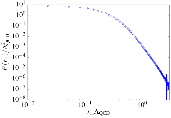
Figure 4: The numerical result for $F(r_{\perp})$ defined in Eq. (59) for $Q_{s}=10\Lambda_{\rm QCD}$ and $m=0$ evaluated in the QDHT algorithm. The error is a $3\sigma$ estimate from the MISER Monte Carlo algorithm.

We choose two values of the saturation momentum as $Q_{s}=5\Lambda_{\rm QCD}\simeq 1\;\text{GeV}$, $Q_{s}=10\Lambda_{\rm QCD}\simeq 2\;\text{GeV}$ and we take the limit of vanishing quark mass $m=0$ for numerical calculations. We calculate $F(r_{\perp})$ by performing the 7-dimensional integration by means of the Monte-Carlo stratified sampling MISER algorithm [35]. In our calculation we use the Python based Scikit-Monaco package. We have sampled $10^{8}$ integration points for each value of $r_{\perp}$. The result for $F(r_{\perp})$ in the case $Q_{s}=10\Lambda_{\rm QCD}$ is shown in Fig. 4.

We have found that $F(r_{\perp})$ rapidly decreases as we increase $r_{\perp}$ which eventually can be attributed to the saturation effect. The Monte Carlo calculation is quite precise for small values of $r_{\perp}$, while the relative error increases as $r_{\perp}$ increases. For $r_{\perp}\Lambda_{\rm QCD}\simeq 3$ the numerical value of the function is already extremely small as $F(3/\Lambda_{\rm QCD})/\Lambda_{\rm QCD}^{2}\simeq 10^{-7}$ up to $10\%$ error. Let us elucidate the actual numerical procedures in more details below.

The angular integration in Eq. (58) defines the Hankel transform for the function $F(r_{\perp})$, i.e.

$$\int d^{2}\boldsymbol{r}_{\perp}\,e^{-i\boldsymbol{k}_{\perp}\cdot\boldsymbol{r}_{\perp}}F(r_{\perp})=2\pi\int_{0}^{\infty}r_{\perp}dr_{\perp}J_{0}(k_{\perp}r_{\perp})F(r_{\perp})\;,$$ (64)

where $J_{0}(x)$ is the zeroth order Bessel function. To calculate the above in practice, we use the numerical method known as the Quasi Discrete Hankel Transform (QDHT) [36]. The computation of the function $F(r_{\perp})$ is performed on a grid corresponding to the points prescribed by the QDHT algorithm. In the case $Q_{s}=10\Lambda_{\rm QCD}$ the maximum value on the grid is chosen as $r^{\text{max}}_{\perp}\Lambda_{\rm QCD}=3$ and for the case $Q_{s}=5\Lambda_{\rm QCD}$ we have taken $r^{\text{max}}_{\perp}\Lambda_{\rm QCD}=6$. The minimal value of $r_{\perp}$ is set by fixing the number of grid points within the QDHT algorithm. In the calculation of $F(r_{\perp})$ we used $10^{2}$ points. We have tested the sensitivity to the cutoffs imposed by the QDHT algorithm. In particular, we confirmed that the results up to $k_{\perp}\simeq 7Q_{s}$ are numerically reliable. This is the maximum value shown in our final numerical results in Fig. 5.

5.2 Discussion of the results

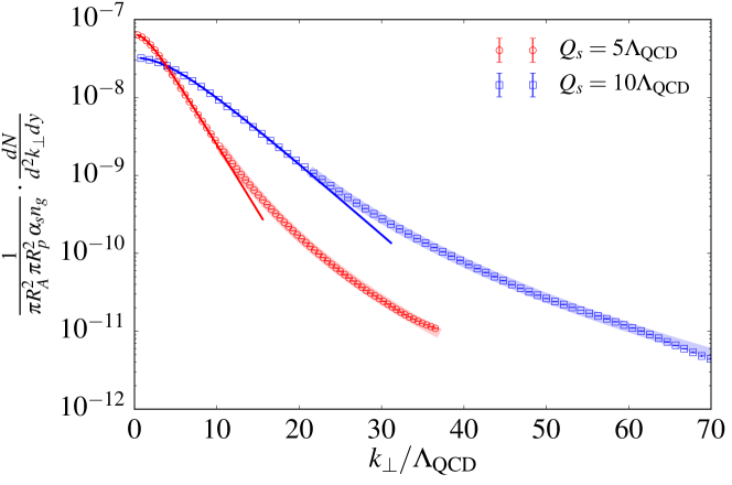
Figure 5: Photon production rate as a function of $k_{\perp}$ in the unit of $\Lambda_{\rm QCD}$ in the limit of vanishing quark mass and for $Q_{s}=5\Lambda_{\rm QCD}$ and $Q_{s}=10\Lambda_{\rm QCD}$. The thin lines represent the exponential fit, while the thick lines with light colors correspond to the power-law type fit.

We show the numerical results for the photon spectrum in Fig. 5 as a function of the transverse momentum $k_{\perp}$. We see that the curve slightly flattens at low momentum, which is attributed to the saturation property. For the results in Fig. 5 we consider the case of a single quark flavor with vanishing quark mass and use $\alpha=1/137$. Although $n_{q}\ll n_{g}\ll Q_{s}^{2}$ by definition of the semi-CGC regime of our present interest, there is some theoretical uncertainty in precisely determining $n_{g}$ of the proton. Thanks to the simple linear dependence on $n_{g}$ as a result of the expansion in terms of $\rho_{p}$, we present our numerical results by scaling $n_{g}$ out entirely.

The data points on Fig. 5 correspond to the results from the QDHT transform, while the solid lines represent the fit results. The soft part of the spectrum up to $k_{\perp}\sim 2Q_{s}$ is very well described with a exponential fitting function, $\exp\bigl{(}-\sqrt{k_{\perp}^{2}+(0.5Q_{s})^{2}}/0.5Q_{s}\bigr{)}$. As an alternative, a Lorentzian-type fitting function, $(k^{2}+(1.3Q_{s})^{2})^{-2.4}$, can work as nicely as the exponential form. The semi-hard part for $k_{\perp}\mathrel{\raise 1.29167pt\hbox{$>$\kern-7.5pt\lower 4.30554pt\hbox{$\sim$}}}2Q_{s}$ can be fitted by the perturbative power-law tail as $(\log(k_{\perp}/Q_{s}))^{1.5}/k_{\perp}^{5.6}$. In Fig. 5 we show the exponential fit by the thin lines and the power-law fit by the thick lines with light colors. In Ref. [9] the Glasma photons would yield a thermal-like spectrum in the $AA$ collisions, and our calculations partially support this for $k_{\perp}\mathrel{\raise 1.29167pt\hbox{$<$\kern-7.5pt\lower 4.30554pt\hbox{$\sim$}}}2Q_{s}$, though a Lorentzian shape can be another choice.

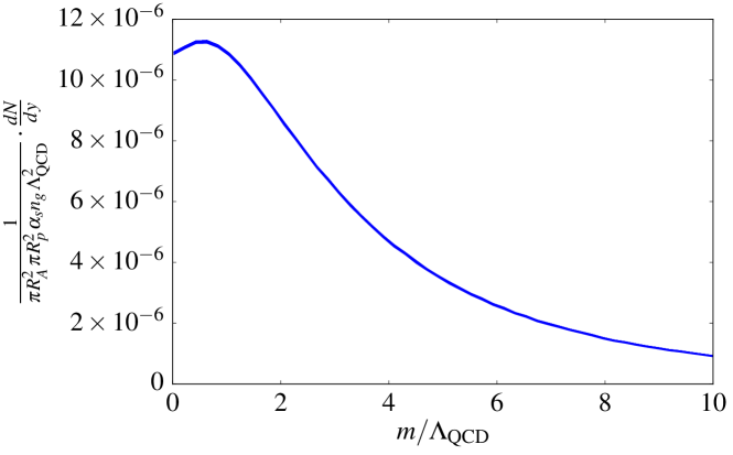
Figure 6: Dependence of the total produced photons $dN/dy$ per unit rapidity on the quark mass $m$. The value $Q_{s}=10\Lambda_{\rm QCD}$ was adopted. The line thickness represents the $3\sigma$ error estimate in the MISER Monte Carlo algorithm.

According to Eq. (58) the number of produced photons $dN/dy$ is given as

$$\frac{1}{\pi R_{A}^{2}\pi R_{p}^{2}\alpha_{s}n_{g}}\cdot\frac{dN}{dy}=\frac{\alpha}{2\pi^{6}}\frac{N_{c}^{2}}{N_{c}^{2}-1}F(0)\;.$$ (65)

In Fig. 6 we show $dN/dy$ as a function of the quark mass for the choice of $Q_{s}=10\Lambda_{\rm QCD}$. We numerically found that the results for $m\mathrel{\raise 1.29167pt\hbox{$>$\kern-7.5pt\lower 4.30554pt\hbox{$\sim$}}}2\Lambda_{\rm QCD}$ can be well fitted by $(\log(m/\Lambda_{\rm QCD}))^{1.8}/m^{2.6}$. From this we can say that the mass dependence is minor for the strange quark, while the photon production is suppressed by a factor $\sim 5$ for the charm quark.

6 Conclusion

In this work we have calculated the photon production rate from the annihilation process with CGC in the $pA$ collision. We have considered a regime where the nucleus is saturated and the proton is more dilute but dominated by gluons over quarks. We have argued that in this semi-CGC regime we should consider a process where the virtual gluon in the proton emits a photon through quark couplings. We have obtained an analytic expression for an annihilation part of the photon rate and identified the part describing saturation physics as the inelastic quadrupole of Wilson lines. We have explicitly demonstrated that the quark loop is both IR and UV finite. Our numerical results can be well fitted with a exponential or a Lorentzian form having a perturbative tail at large momenta. The contribution of Bremsstrahlung photons, shown in diagrams (a) and (b) in Fig. 1, must be explicitly included in the future phenomenological application.

The multiple scattering effects are included through the MV model but the small $x$ evolution effects are not yet covered. However, the main formula for the photon production rate as given in Eq. (44) is quite general and amenable to such systematic improvements. In particular, the simple dipole model considered here could be replaced by the solution of the rcBK equation for future updates [31].

To our best knowledge this is the first full numerical integration over the inelastic quadrupole. In Ref. [27] the inelastic quadrupole was necessary to predict the singlet quarkonium production. However, in the explicit calculations the authors have used an approximate factorized Ansatz for the quadrupole in terms of products of dipoles. Thus, our numerical schemes may have some other useful applications for related subjects.

Also, the CGC-type quark-loop diagrams, such as the case discussed here, can in principle be sensitive to the quantum anomaly. In view of the possible connection between strong external magnetic fields and the local parity violation accommodated in the CGC initial state and the glasma evolution [37, 38] our calculation may be of a broader interest giving a microscopic foundation of anomaly-induced photons in the early dynamics of the heavy-ion collision [39, 40]. This is one of intriguing directions for future studies.

For the next step as a continuation from the present work, we plan to perform a more detailed analysis with physical masses of $u$, $d$, $s$, and $c$ quarks. Such a treatment will be indispensable because quark-loop contributions are sensitive to the explicit breaking of three ($u$, $d$, $s$) flavor degeneracy. By including also the Bremsstrahlung contributions, we can complete the systematic calculation of photon from CGC in the $pA$ collision and make a full quantitative prediction/comparison to experimental data.

Appendix A Ward identity

As an independent check, we explicitly show that the photon amplitude (32) satisfies the Ward identity. To that end, we must replace $\epsilon_{\lambda}^{\mu}(\boldsymbol{k})\to k^{\mu}$ in the Dirac trace (30). We have

$$\begin{split}&{\rm Tr}_{D}\bigl{[}\hbox to0.0pt{\hbox to5.52084pt{\hfil/\hfil}\hss}k(\hbox to0.0pt{\hbox to5.00002pt{\hfil$q$\hfil}\hss}/+m)\hbox to0.0pt{\hbox to6.00235pt{\hfil/\hfil}\hss}n(\hbox to0.0pt{\hbox to5.00002pt{\hfil$q$\hfil}\hss}/-\hbox to0.0pt{\hbox to5.03125pt{\hfil/\hfil}\hss}p^{\prime}+m)\boldsymbol{p}_{\perp}\cdot\boldsymbol{\gamma}_{\perp}(\hbox to0.0pt{\hbox to5.00002pt{\hfil$q$\hfil}\hss}/-\hbox to0.0pt{\hbox to5.03125pt{\hfil/\hfil}\hss}p-\hbox to0.0pt{\hbox to5.03125pt{\hfil/\hfil}\hss}p^{\prime}+m)\hbox to0.0pt{\hbox to6.00235pt{\hfil/\hfil}\hss}n(\hbox to0.0pt{\hbox to5.00002pt{\hfil$q$\hfil}\hss}/-\hbox to0.0pt{\hbox to5.52084pt{\hfil/\hfil}\hss}k+m)\bigr{]}\\ &=8p^{+2}\bigl{[}xp_{\perp}^{2}-2a(x)\boldsymbol{p}_{\perp}\cdot(\boldsymbol{q}_{\perp}-\boldsymbol{p}_{\perp}^{\prime})\bigr{]}\bigl{[}(x\boldsymbol{k}_{\perp}-\boldsymbol{q}_{\perp})^{2}+m^{2}\bigr{]}\\ &=8p^{+2}\bigl{[}\frac{1}{2}p_{\perp}^{2}+2a(x)\boldsymbol{p}_{\perp}\cdot\boldsymbol{l}_{\perp}\bigr{]}\bigl{[}(x\boldsymbol{k}_{\perp}-\boldsymbol{q}_{\perp})^{2}+m^{2}\bigr{]}~{},\end{split}$$ (66)

where in the second line we have introduced a substitution $\boldsymbol{p}_{\perp}^{\prime}\to\boldsymbol{l}_{\perp}=\boldsymbol{p}_{\perp}^{\prime}-\boldsymbol{q}_{\perp}+\boldsymbol{p}_{\perp}/2$ and where $a(x)=x-\frac{1}{2}$. Defining $\mathcal{M}_{\lambda}(\boldsymbol{k})=\epsilon^{\mu}_{\lambda}(\boldsymbol{k})\mathcal{T}^{\mu}(\boldsymbol{k})$ and using the results of Sec. 3.3 we have

$$\begin{split}k_{\mu}\mathcal{T}^{\mu}(\boldsymbol{k})&=\frac{eg}{\pi}\int_{0}^{1}dx\int\frac{d^{2}\boldsymbol{p}_{\perp}}{(2\pi)^{2}}\frac{d^{2}\boldsymbol{l}_{\perp}}{(2\pi)^{2}}\frac{d^{2}\boldsymbol{q}_{\perp}}{(2\pi)^{2}}\,\frac{1}{p_{\perp}^{2}}\\ &\times\frac{1}{(x\boldsymbol{k}_{\perp}-\boldsymbol{q}_{\perp})^{2}+m^{2}}\,\frac{1}{[a(x)\boldsymbol{p}_{\perp}+\boldsymbol{l}_{\perp}]^{2}+m_{p}^{2}(x)}\\ &\times\bigl{[}\frac{1}{2}p_{\perp}^{2}+2a(x)\boldsymbol{p}_{\perp}\cdot\boldsymbol{l}_{\perp}\bigr{]}\bigl{[}(x\boldsymbol{k}_{\perp}-\boldsymbol{q}_{\perp})^{2}+m^{2}\bigr{]}\\ &\times\text{Tr}_{c}\biggl{[}U\left(\boldsymbol{l}_{\perp}+\boldsymbol{q}_{\perp}-\frac{\boldsymbol{p}_{\perp}}{2}\right)\,\rho_{p}(\boldsymbol{p}_{\perp})\,U^{\dagger}\left(\boldsymbol{l}_{\perp}+\boldsymbol{q}_{\perp}+\frac{\boldsymbol{p}_{\perp}}{2}-\boldsymbol{k}_{\perp}\right)\biggr{]}\\ &=\int_{0}^{1}dx\int\frac{d^{2}\boldsymbol{p}_{\perp}}{(2\pi)^{2}}\frac{d^{2}\boldsymbol{l}_{\perp}}{(2\pi)^{2}}\,\frac{1}{p_{\perp}^{2}}\,\frac{\frac{1}{2}p_{\perp}^{2}+2a(x)\boldsymbol{p}_{\perp}\cdot\boldsymbol{l}_{\perp}}{[a(x)\boldsymbol{p}_{\perp}+\boldsymbol{l}_{\perp}]^{2}+m_{p}^{2}(x)}\\ &\times\int d^{2}\boldsymbol{y}_{\perp}e^{i(\boldsymbol{p}_{\perp}-\boldsymbol{k}_{\perp})\cdot\boldsymbol{y}_{\perp}}\text{Tr}_{c}\bigl{[}U(\boldsymbol{y}_{\perp})\,\rho_{p}(\boldsymbol{p}_{\perp})\,U^{\dagger}(\boldsymbol{y}_{\perp})\bigr{]}\\ &=\frac{\text{Tr}_{c}[\rho_{p}(\boldsymbol{k}_{\perp})]}{k_{\perp}^{2}}\int_{0}^{1}dx\int\frac{d^{2}\boldsymbol{l}_{\perp}}{(2\pi)^{2}}\,\frac{\frac{1}{2}k_{\perp}^{2}+2a(x)\boldsymbol{k}_{\perp}\cdot\boldsymbol{l}_{\perp}}{[a(x)\boldsymbol{k}_{\perp}+\boldsymbol{l}_{\perp}]^{2}+m_{k}^{2}(x)}~{},\end{split}$$ (67)

which vanishes because of the color trace. In the second line we have recognized that, due to the cancellation between the numerator and the denominator, the dependence of $\boldsymbol{q}_{\perp}$ comes only through the Wilson lines. Fourier transforming the Wilson lines to coordinate space we have performed the $\boldsymbol{q}_{\perp}$ integration. In the third line we have performed the $\boldsymbol{y}_{\perp}$ integration.

Appendix B Angular integrations

Here we perform the integration over the polar angle $\phi_{p}$ associated with the gluon momentum $\boldsymbol{p}_{\perp}$ in Eq. (44). We use the following formulas

$$\begin{split}&\int_{0}^{2\pi}d\phi_{p}e^{i\boldsymbol{p}_{\perp}\cdot\boldsymbol{r}_{\perp}}=2\pi J_{0}(p_{\perp}r_{\perp})~{},\\ &\int_{0}^{2\pi}d\phi_{p}\,\boldsymbol{a}_{\perp}\cdot\hat{\boldsymbol{p}}_{\perp}\,e^{i\boldsymbol{p}_{\perp}\cdot\boldsymbol{r}_{\perp}}=2\pi i(\boldsymbol{a}_{\perp}\cdot\hat{\boldsymbol{r}}_{\perp})J_{1}(p_{\perp}r_{\perp})~{},\\ &\int_{0}^{2\pi}d\phi_{p}(\boldsymbol{a}_{\perp}\cdot\hat{\boldsymbol{p}}_{\perp})(\boldsymbol{b}\cdot\hat{\boldsymbol{p}}_{\perp})e^{i\boldsymbol{p}_{\perp}\cdot\boldsymbol{r}_{\perp}}=2\pi(\boldsymbol{a}_{\perp}\cdot\hat{\boldsymbol{r}}_{\perp})(\boldsymbol{b}\cdot\hat{\boldsymbol{r}}_{\perp})J_{0}(p_{\perp}r_{\perp})\\ &+2\pi\bigl{[}\boldsymbol{a}_{\perp}\cdot\boldsymbol{b}-2(\boldsymbol{a}_{\perp}\cdot\hat{\boldsymbol{r}}_{\perp})(\boldsymbol{b}\cdot\hat{\boldsymbol{r}}_{\perp})\bigr{]}\frac{J_{1}(p_{\perp}r_{\perp})}{p_{\perp}r_{\perp}}~{}.\end{split}$$ (68)

where $J_{0,1}(x)$ are Bessel functions of the zeroth and the first order, respectively.

We define the auxiliary functions

$$\begin{split}\varphi_{\mu\nu\rho}^{\alpha}(x,x^{\prime},\boldsymbol{u}_{\perp},\boldsymbol{u}_{\perp}^{\prime},\boldsymbol{r}_{\perp})&=\int_{0}^{\infty}\frac{\varphi(p_{\perp})\,p_{\perp}^{\alpha+2}dp_{\perp}}{(p_{\perp}^{2}+\Lambda_{\rm QCD}^{2})^{2}}\,m_{p}^{\mu}(x)m_{p}^{\nu}(x^{\prime})\\ &\times K_{\mu}(m_{p}(x)u_{\perp})\,K_{\nu}(m_{p}(x^{\prime})u^{\prime}_{\perp})\,J_{\rho}(p_{\perp}r_{\perp})~{},\end{split}$$ (69)

where $\mu$, $\nu$, $\rho$, $\alpha$ $\in\mathbb{N}_{0}$. The angular integration of the first term in Eq. (44) gives

$$\begin{split}&\frac{1}{2\pi}\int d^{2}\boldsymbol{p}_{\perp}\frac{p_{\perp}^{4}\varphi_{p}(p_{\perp})}{(p_{\perp}^{2}+\Lambda_{\rm QCD}^{2})^{2}}\,e^{i\boldsymbol{p}_{\perp}\cdot\boldsymbol{r}_{\perp}}\Psi_{1}\Psi^{\prime*}_{1}=16m^{2}b(x)b(x^{\prime})K_{1}(mu_{\perp})K_{1}(mu^{\prime}_{\perp})\\ &\times\biggl{\{}a(x)a(x^{\prime})\varphi_{000}^{5}+(\hat{\boldsymbol{u}}_{\perp}\cdot\hat{\boldsymbol{r}}_{\perp})(\hat{\boldsymbol{u}}_{\perp}^{\prime}\cdot\hat{\boldsymbol{r}}_{\perp})\varphi_{110}^{3}\\ &+\bigl{[}\hat{\boldsymbol{u}}_{\perp}\cdot\hat{\boldsymbol{u}}_{\perp}^{\prime}-2(\hat{\boldsymbol{u}}_{\perp}\cdot\hat{\boldsymbol{r}}_{\perp})(\hat{\boldsymbol{u}}_{\perp}^{\prime}\cdot\hat{\boldsymbol{r}}_{\perp})\bigr{]}\frac{1}{r_{\perp}}\varphi_{111}^{2}-2a(x^{\prime})(\hat{\boldsymbol{u}}_{\perp}^{\prime}\cdot\hat{\boldsymbol{r}}_{\perp})\varphi_{011}^{4}\biggr{\}}~{},\end{split}$$ (70)

where for simplicity we suppressed the variables on $\varphi_{\mu\nu\rho}^{\alpha}$. Likewise, the second and the third term in Eq. (44) are calculated to give

$$\begin{split}&\frac{1}{2\pi}\int d^{2}\boldsymbol{p}_{\perp}\frac{p_{\perp}^{4}\varphi_{p}(p_{\perp})}{(p_{\perp}^{2}+\Lambda_{\rm QCD}^{2})^{2}}\,e^{i\boldsymbol{p}_{\perp}\cdot\boldsymbol{r}_{\perp}}\Psi_{2}\Psi^{\prime*}_{2}=m^{2}\bigl{[}K_{1}(mu_{\perp})K_{1}(mu^{\prime}_{\perp})\varphi_{110}^{3}\\ &\qquad+m^{2}K_{0}(mu_{\perp})K_{0}(mu^{\prime}_{\perp})\varphi_{000}^{3}+2mK_{1}(mu_{\perp})K_{0}(mu^{\prime}_{\perp})\varphi_{100}^{3}\bigr{]}~{},\end{split}$$ (71)

$$\begin{split}&\frac{1}{2\pi}\int d^{2}\boldsymbol{p}_{\perp}\frac{p_{\perp}^{4}\varphi_{p}(p_{\perp})}{(p_{\perp}^{2}+\Lambda_{\rm QCD}^{2})^{2}}\,e^{i\boldsymbol{p}_{\perp}\cdot\boldsymbol{r}_{\perp}}\,\hat{\boldsymbol{u}}_{\perp}\cdot\hat{\boldsymbol{p}}_{\perp}\Psi_{1}\Psi^{\prime*}_{2}=4m^{2}b(x)K_{1}(mu_{\perp})\\ &\qquad\times\biggl{\{}a(x)\,\hat{\boldsymbol{u}}_{\perp}\cdot\hat{\boldsymbol{r}}_{\perp}\bigl{[}K_{1}(mu^{\prime}_{\perp})\varphi_{011}^{4}+mK_{0}(mu^{\prime}_{\perp})\varphi_{001}^{4}\bigr{]}\\ &\qquad-K_{1}(mu^{\prime}_{\perp})\bigl{[}(\hat{\boldsymbol{u}}_{\perp}\cdot\hat{\boldsymbol{r}}_{\perp})^{2}\varphi_{110}^{3}+\bigl{(}1-2(\hat{\boldsymbol{u}}_{\perp}\cdot\hat{\boldsymbol{r}}_{\perp})^{2}\bigr{)}\frac{1}{r_{\perp}}\varphi_{111}^{2}\bigr{]}\\ &\qquad-mK_{0}(mu^{\prime}_{\perp})\bigl{[}(\hat{\boldsymbol{u}}_{\perp}\cdot\hat{\boldsymbol{r}}_{\perp})^{2}\varphi_{100}^{3}+\bigl{(}1-2(\hat{\boldsymbol{u}}_{\perp}\cdot\hat{\boldsymbol{r}}_{\perp})^{2}\bigr{)}\frac{1}{r_{\perp}}\varphi_{101}^{2}\bigr{]}\biggr{\}}~{}.\end{split}$$ (72)

Appendix C Inelastic quadrupole in the MV model

The color average of the inelastic quadrupole $S(\boldsymbol{y}_{\perp},\boldsymbol{z}_{\perp},\boldsymbol{y}_{\perp}^{\prime},\boldsymbol{z}_{\perp}^{\prime})$ (see Eq. (41)) within the MV model is calculated by the use of the techniques described in [18, 33, 34]. We closely follow the general procedure described in Ref. [34] to which we refer the reader for more details. In the notation of [34] the expression for the Wilson line product is written as

$$\begin{split}&S(\boldsymbol{y}_{\perp},\boldsymbol{z}_{\perp},\boldsymbol{y}_{\perp}^{\prime},\boldsymbol{z}_{\perp}^{\prime})=\frac{1}{N_{c}}\big{\langle}{\rm Tr}\left[U(\boldsymbol{y}_{\perp})T_{F}^{a}U^{\dagger}(\boldsymbol{z}_{\perp})\right]{\rm Tr}\left[U(\boldsymbol{y}_{\perp}^{\prime})T^{a}U^{\dagger}(\boldsymbol{z}_{\perp}^{\prime})\right]\big{\rangle}\\ &=\frac{1}{N_{c}}\delta_{\beta_{1}\beta_{2}}\delta_{\beta_{3}\beta_{4}}T_{F\alpha_{1}\alpha_{2}}^{a}T_{F\alpha_{3}\alpha_{4}}^{a}\left\langle U_{\beta_{1}\alpha_{1}}(\boldsymbol{y}_{\perp})U^{*}_{\beta_{2}\alpha_{2}}(\boldsymbol{z}_{\perp})U_{\beta_{3}\alpha_{3}}(\boldsymbol{y}_{\perp}^{\prime})U^{*}_{\beta_{4}\alpha_{4}}(\boldsymbol{z}_{\perp}^{\prime})\right\rangle\\ &=\frac{1}{N_{c}}\delta_{\beta_{1}\beta_{2}}\delta_{\beta_{3}\beta_{4}}T_{F\alpha_{1}\alpha_{2}}^{a}T_{F\alpha_{3}\alpha_{4}}^{a}\langle\beta_{1}\beta_{2}\beta_{3}\beta_{4}|e^{-(H_{0}+V)}|\alpha_{1}\alpha_{2}\alpha_{3}\alpha_{4}\rangle~{},\end{split}$$ (73)

where [34]

$$H_{0}=\frac{2N_{c}}{N_{c}^{2}-1}(T_{F1}^{a}-T_{F2}^{a*}+T_{F3}^{a}-T_{F4}^{a*})^{2}L(0)~{},$$ (74)

$$\begin{split}V=-\frac{2N_{c}}{N_{c}^{2}-1}\bigl{[}&-T_{F2}^{a*}T_{F1}^{a}B_{2}(|\boldsymbol{y}_{\perp}-\boldsymbol{z}_{\perp}|)+T_{F3}^{a}T_{F1}^{a}B_{2}(|\boldsymbol{y}_{\perp}-\boldsymbol{y}_{\perp}^{\prime}|)\\ &-T_{F3}^{a}T_{F2}^{a*}B_{2}(|\boldsymbol{z}_{\perp}-\boldsymbol{y}_{\perp}^{\prime}|)-T_{F4}^{a*}T_{F1}^{a}B_{2}(|\boldsymbol{y}_{\perp}-\boldsymbol{z}_{\perp}^{\prime}|)\\ &+T_{F4}^{a*}T_{F2}^{a*}B_{2}(|\boldsymbol{z}_{\perp}-\boldsymbol{z}_{\perp}^{\prime}|)-T_{F4}^{a*}T_{F3}^{a}B_{2}(|\boldsymbol{y}_{\perp}^{\prime}-\boldsymbol{z}_{\perp}^{\prime}|)\bigr{]}~{}.\end{split}$$ (75)

Here

$$L(|\boldsymbol{x}_{\perp}-\boldsymbol{y}_{\perp}|)=Q_{s}^{2}\int d^{2}\boldsymbol{z}_{\perp}G_{0}(\boldsymbol{x}_{\perp}-\boldsymbol{z}_{\perp})G_{0}(\boldsymbol{y}_{\perp}-\boldsymbol{z}_{\perp})~{},$$ (76)

with $G_{0}(\boldsymbol{x}_{\perp})$ a Green function of a $2D$ Laplacian

$$\partial_{\boldsymbol{x}_{\perp}}^{2}G_{0}(\boldsymbol{x}_{\perp})=\delta^{(2)}(\boldsymbol{x}_{\perp})~{},$$ (77)

and

$$B_{2}(|\boldsymbol{x}_{\perp}-\boldsymbol{y}_{\perp}|)=2L(0)-2L(\boldsymbol{x}_{\perp}-\boldsymbol{y}_{\perp})~{}.$$ (78)

Define now $|\alpha\rangle\equiv|\alpha_{1}\alpha_{2}\alpha_{3}\alpha_{4}\rangle$. The Wilson line product has two singlets, defined as

$$\langle\alpha|s_{1}\rangle=\frac{1}{N_{c}}\delta_{\alpha_{1}\alpha_{2}}\delta_{\alpha_{3}\alpha_{4}}~{},\qquad\langle\alpha|s_{2}\rangle=\frac{2}{\sqrt{N_{c}^{2}-1}}T_{F\alpha_{1}\alpha_{2}}^{a}T_{F\alpha_{3}\alpha_{4}}^{a}~{},$$ (79)

Note that precisely these singlets appear in the contraction of the Wilson line product (73). This leads to

$$\begin{split}S(\boldsymbol{y}_{\perp},\boldsymbol{z}_{\perp},\boldsymbol{y}_{\perp}^{\prime},\boldsymbol{z}_{\perp}^{\prime})&=\frac{\sqrt{N_{c}^{2}-1}}{2}\sum_{\alpha,\beta}\langle s_{1}|\beta\rangle\langle\beta|e^{-(H_{0}+V)}|\alpha\rangle\langle\alpha|s_{2}\rangle\\ &=\frac{\sqrt{N_{c}^{2}-1}}{2}\langle s_{1}|e^{-V}|s_{2}\rangle~{},\end{split}$$ (80)

where in the first line we used the definition of the singlets (79). In the second line we have used $H_{0}|s_{1,2}\rangle=0$. From [34] (see also [18]), we have

$$\langle s_{1}|e^{-V}|s_{2}\rangle=-\frac{2V_{12}}{\phi}e^{-\frac{1}{2}{\rm Tr}V}\sinh\frac{\phi}{2}~{},$$ (81)

where the $2\times 2$ matrix $V_{ij}=\langle s_{i}|V|s_{j}\rangle$ is given as [34]

$$\begin{pmatrix}V_{11}&V_{12}\\ V_{21}&V_{22}\end{pmatrix}=-\frac{2N_{c}}{N_{c}^{2}-1}\begin{pmatrix}-\frac{N_{c}^{2}-1}{N_{c}}\gamma&\frac{\sqrt{N_{c}^{2}-1}}{N_{c}}(\beta-\alpha)\\ \frac{\sqrt{N_{c}^{2}-1}}{N_{c}}(\beta-\alpha)&\frac{1}{N_{c}}(\gamma-2\beta+(2-N_{c}^{2})\alpha)\end{pmatrix}~{}.$$ (82)

The functions $\alpha$, $\beta$ and $\gamma$ were defined in Eq. (52) and $\phi=\sqrt{({\rm tr}V)^{2}-4{\rm det}V}$. A simple algebraic manipulation of (81) leads to

$$\begin{split}S(\boldsymbol{y}_{\perp},\boldsymbol{z}_{\perp},\boldsymbol{y}_{\perp}^{\prime},\boldsymbol{z}_{\perp}^{\prime})&=\frac{1}{N_{c}}\frac{(N_{c}^{2}-1)(\beta-\alpha)}{\sqrt{N_{c}^{2}(\alpha-\gamma)^{2}-4(\alpha-\beta)(\beta-\gamma)}}\\ &\times\exp\biggl{[}-\frac{2\beta+(\alpha+\gamma)(N_{c}^{2}-2)}{N_{c}^{2}-1}\biggr{]}\\ &\times\sinh\biggl{[}\frac{N_{c}}{N_{c}^{2}-1}\sqrt{N_{c}^{2}(\alpha-\gamma)^{2}-4(\alpha-\beta)(\beta-\gamma)}\biggr{]}\;.\end{split}$$ (83)

References

References

• [1] L. D. McLerran and R. Venugopalan, Phys. Rev. D 49 (1994) 2233 [hep-ph/9309289]; Phys. Rev. D 49 (1994) 3352 [hep-ph/9311205]; Phys. Rev. D 50 (1994) 2225 [hep-ph/9402335].
• [2] A. M. Stasto, K. J. Golec-Biernat and J. Kwiecinski, Phys. Rev. Lett.  86 (2001) 596 [hep-ph/0007192].
• [3] K. Fukushima, Acta Phys. Polon. B 42 (2011) 2697 [hep-ph/1111.1025].
• [4] F. Gelis, Nucl. Phys. A 931 (2014) 73 [hep-ph/1412.0471].
• [5] J. L. Albacete and C. Marquet, Prog. Part. Nucl. Phys.  76 (2014) 1 [hep-ph/1401.4866].
• [6] A. Adare et al. [PHENIX Collaboration], Phys. Rev. Lett.  104 (2010) 132301 [nucl-ex/0804.4168]; M. Wilde [ALICE Collaboration], Nucl. Phys. A 904-905 (2013) 573c [arXiv:1210.5958 [hep-ex]].
• [7] M. Klasen, C. Klein-Bösing, F. König and J. P. Wessels, JHEP 1310 (2013) 119 [arXiv:1307.7034 [hep-ph]].
• [8] C. Klein-Bösing and L. McLerran, Phys. Lett. B 734 (2014) 282 [arXiv:1403.1174 [nucl-th]].
• [9] L. McLerran and B. Schenke, Nucl. Phys. A 929 (2014) 71 [hep-ph/1403.7462].
• [10] R. Baier, H. Nakkagawa, A. Niegawa and K. Redlich, Z. Phys. C 53 (1992) 433.
• [11] M. Heffernan, P. Hohler and R. Rapp, Phys. Rev. C 91 (2015) 2, 027902 [hep-ph/1411.7012].
• [12] F. Gelis and J. Jalilian-Marian, Phys. Rev. D 66 (2002) 014021 [hep-ph/0205037], J. Jalilian-Marian, Nucl. Phys. A 753 (2005) 307 [hep-ph/0501222], J. Jalilian-Marian and A. H. Rezaeian, Phys. Rev. D 86 (2012) 034016 [hep-ph/1204.1319].
• [13] N. Tanji, Phys. Rev. D 92 (2015) 12, 125012 [hep-ph/1506.08442].
• [14] A. Dumitru and L. D. McLerran, Nucl. Phys. A 700 (2002) 492 [hep-ph/0105268].
• [15] J. P. Blaizot, F. Gelis and R. Venugopalan, Nucl. Phys. A 743 (2004) 13 [hep-ph/0402256].
• [16] F. Gelis and Y. Mehtar-Tani, Phys. Rev. D 73 (2006) 034019 [hep-ph/0512079].
• [17] K. Fukushima and Y. Hidaka, Nucl. Phys. A 813 (2008) 171 [hep-ph/0806.2143].
• [18] J. P. Blaizot, F. Gelis and R. Venugopalan, Nucl. Phys. A 743 (2004) 57 [hep-ph/0402257], H. Fujii, F. Gelis and R. Venugopalan, Nucl. Phys. A 780 (2006) 146 [hep-ph/0603099].
• [19] A. Adare et al., Phys. Rev. C 87 (2013) 054907 [nucl-ex/1208.1234].
• [20] C. Shen, J.-F. Paquet, G. S. Denicol, S. Jeon and C. Gale, [nucl-th/1504.07989].
• [21] See a Quark Matter 2015 poster contribution from the ALICE Collaboration; https://indico.cern.ch/event/355454/session/33/contribution/303.
• [22] Y. V. Kovchegov, Phys. Rev. D 54 (1996) 5463 [hep-ph/9605446].
• [23] A. J. Baltz and L. D. McLerran, Phys. Rev. C 58 (1998) 1679 [nucl-th/9804042], L. D. McLerran and R. Venugopalan, Phys. Rev. D 59 (1999) 094002 [hep-ph/9809427].
• [24] R. Mertig, M. Böhm, and A. Denner, Comput. Phys. Commun. 64 (1991) 345– 359, V. Shtabovenko, R. Mertig and F. Orellana, [hep-ph/1601.01167].
• [25] F. Dominguez, C. Marquet, B. W. Xiao and F. Yuan, Phys. Rev. D 83 (2011) 105005 [hep-ph/1101.0715].
• [26] J. Jalilian-Marian and Y. V. Kovchegov, Phys. Rev. D 70 (2004) 114017 Erratum: [Phys. Rev. D 71 (2005) 079901] [hep-ph/0405266].
• [27] Z. B. Kang, Y. Q. Ma and R. Venugopalan, JHEP 1401 (2014) 056 [hep-ph/1309.7337], Y. Q. Ma and R. Venugopalan, Phys. Rev. Lett.  113 (2014) no.19, 192301 [hep-ph/1408.4075].
• [28] I. Balitsky, Nucl. Phys. B 463 (1996) 99 [hep-ph/9509348].
• [29] J. Jalilian-Marian, A. Kovner, A. Leonidov and H. Weigert, Nucl. Phys. B 504 (1997) 415 [hep-ph/9701284], Phys. Rev. D 59 (1998) 014014 [hep-ph/9706377], E. Iancu, A. Leonidov and L. D. McLerran, Nucl. Phys. A 692 (2001) 583 [hep-ph/0011241].
• [30] Y. V. Kovchegov, Phys. Rev. D 61 (2000) 074018 [hep-ph/9905214].
• [31] J. L. Albacete and Y. V. Kovchegov, Phys. Rev. D 75 (2007) 125021 [hep-ph/0704.0612].
• [32] E. Iancu and D. N. Triantafyllopoulos, JHEP 1204 (2012) 025 [hep-ph/1112.1104], A. Dumitru, J. Jalilian-Marian, T. Lappi, B. Schenke and R. Venugopalan, Phys. Lett. B 706 (2011) 219 [hep-ph/1108.4764].
• [33] F. Gelis and A. Peshier, Nucl. Phys. A 697 (2002) 879 [hep-ph/0107142].
• [34] K. Fukushima and Y. Hidaka, JHEP 0706 (2007) 040 [hep-ph/0704.2806].
• [35] W. H. Press, S. A. Teukolsky, W. T. Vetterling and B. P. Flannery, Numerical Recipes in FORTRAN: The Art of Scientific Computing, ISBN-9780521430647.
• [36] L. Yu, M. Huang, M. Chen, W. Chen, W. Huang, and Z. Zhu, Opt. Lett.   23 (1998) 409-411.
• [37] D. Kharzeev, A. Krasnitz and R. Venugopalan, Phys. Lett. B 545 (2002) 298 [hep-ph/0109253].
• [38] M. Mace, S. Schlichting and R. Venugopalan, [hep-ph/1601.07342].
• [39] G. Basar, D. Kharzeev, D. Kharzeev and V. Skokov, Phys. Rev. Lett.  109 (2012) 202303 [hep-ph/1206.1334].
• [40] K. Fukushima and K. Mameda, Phys. Rev. D 86, 071501 (2012) [hep-ph/1206.3128].