On the inconsistency between cosmic stellar mass density and star formation rate up to $z\sim 8$

Abstract

In this paper, we test the discrepancy between the stellar mass density and instantaneous star formation rate in redshift range $0<z<8$ using a large observational data sample. We first compile the measurements of the stellar mass densities up to $z\sim 8$. Comparing the observed stellar mass densities with the time-integral of instantaneous star formation history, we find that the observed stellar mass densities are lower than that implied from star formation history at $z<4$. We also use Markov chain monte carlo method to derive the best-fitting star formation history from the observed stellar mass density data. At $0.5<z<6$, the observed star formation rate densities are larger than the best-fitting one, especially at $z\sim 2$ where by a factor of about two. However, at lower ($z<0.5$) and higher redshifts ($z>6$), the derived star formation history is consistent with the observations. This is the first time to test the discrepancy between the observed stellar mass density and instantaneous star formation rate up to very high redshift $z\approx 8$ using the Markov chain monte carlo method and a varying recycling factor. Several possible reasons for this discrepancy are discussed, such as underestimation of stellar mass density, initial mass function and cosmic metallicity evolution.

1 Introduction

Thanks to the development of the telescopes, more and more important and accurate data are obtained in almost all fields of astronomy. The multi-wavelength observations with Hubble, Spitzer Space Telescopes and other large ground-base telescopes give us much information of high redshift galaxies. It gives us a great chance to measure the stellar mass density (SMD) from galaxy surveys (Labbé et al., 2013; Santini et al., 2015; Grazian et al., 2015, hereafter G15) and instantaneous star formation rate density (SFRD) (Bouwens et al., 2012a, b; Schenker et al., 2013) up to about $z=8$. Because of the physical connection between the star formation history (SFH) and SMD, we expect that these two measured quantities should be consistent with each other.

Integrating the instantaneous SFH over redshift and making some correction for the mass-loss during the stellar evolution through stellar winds and explosion processes (Renzini & Voli, 1981; Woosley & Weaver, 1995), we can get the predicted stellar mass density history (SMH). Meanwhile, after the same stellar evolution correction, the SFH can be obtained from derivative of SMH by redshift. Just as mentioned above, both of the SFH and SMH can be measured independently. So one can compare them to check whether the instantaneous SFH and SMH are consistent with each other. However, in order to make a reasonable comparison, the SFH and SMH should be derived under same assumptions, such as initial mass function (IMF), metallicity and dust correction. Furthermore, to get the unbiased SFH and SMH, we also need to obtain the correct SFRD and SMD calibration respectively. Because all of these factors can affect the final comparison result (G15; Hopkins & Beacom, 2006; Wilkins et al., 2008; Madau & Dickinson, 2014).

Numerous studies have been done to compare those two quantities, but their results are not consistent with each other. For example, some authors have found that there is a good agreement between the measured SFH and SMH (Madau et al., 1998; Fontana et al., 2004; Arnouts et al., 2007; Reddy, 2011; Behroozi et al., 2013). Reddy (2011) found that the SFH and SMH had a general agreement with each other if considering some systematic effects, such as the evolution of the UV luminosity function of galaxy, stellar mass in UV faint galaxies and the dust attenuation varying with luminosity. Behroozi et al. (2013) constrained the SFH and SMH based on the stellar mass-halo mass relation and found that both SMH and SFH are consistent with observations. On the contrary, other authors have found that there is puzzling disagreement between them (G15; Hopkins & Beacom, 2006; Wilkins et al., 2008; Santini et al., 2012; Madau & Dickinson, 2014). Hopkins & Beacom (2006) (hereafter, HB06) found that the SMH inferred from the best-fitting SFH is larger than the observed one over redshift $z<3$, and the larger factor peaked at redshift $z\sim 2$ is about four. Wilkins et al. (2008) (hereafter, W08) compared the SMD and SFRD in redshift $z\leq 4$. They found the derived SFH from observed SMH is lower than the observed SFH and the discrepancy peaks at $z\sim 3$ by 0.6 dex. Madau & Dickinson (2014) (hereafter, MD14) have also found this discrepancy, although it is not so significant. They have found that the inferred SMD history was larger than the observed one by a factor about only 60%. However, these work used different stellar IMF assumptions. HB06 used the IMFs, noted as BG IMF and SalA IMF in HB06, given in Baldry & Glazebrook (2003). W08 defined a new IMF with low-mass slope of -1.0 ($0.1\,M_{\odot}<M<0.5\,M_{\odot}$), and used this IMF in their work. While MD14 used a traditional Salpeter IMF with slope of -2.35. The choices of IMF can lead to some deviations in the comparison, which we will show in the discussion section. Several explanations are proposed for this discrepancy, including underestimation of the stellar mass (Maraston et al., 2010; Bernardi et al., 2013; Courteau et al., 2014). Instead, some authors claimed that the observed SFRD is overestimated in UV and IR band (Utomo et al., 2014) or FUV and U band (Boquien et al., 2014). Alternatively, a possible evolution of stellar IMF will also affect the estimations of observed SFH and SMH (HB06; W08). Because this discrepancy is still under debate, we use a large observed SFRD and SMD data, including the latest observations, to reinvestigate this problem by using Markov chain monte carlo (MCMC) method and considering the stellar evolution effect in a more detailed way.

The structure of this paper is organized as follows. We will give an introduction of the SMD and SFH in section 2 and 3 respectively. In section 4, we will introduce our method and give our result. Some potential causes for the discrepancy between observed SFH and SMH are discussed in section 5. Finally, summary will be given in section 6. For simplicity, we assume the Salpeter IMF with index of -2.35 (Salpeter, 1955) and solar metallicity as a universal metallicity in our work. The flat $\Lambda$CDM cosmology with $h=0.7$ and $\Omega_{m}=0.3$ is adopted.

2 The Stellar Mass Density

The SMD $\rho_{*}(z)$ is the stellar mass in a unit co-moving cosmic volume at redshift $z$. It can be obtained by integrating the galaxy stellar mass function (GSMF) $\Psi(M)$ at a certain redshift,

$$\rho_{*}(z)=\int^{\infty}_{0}M\Psi_{z}(M)~{}dM,$$ (1)

where $\Psi(M)~{}dM$ represents the number of galaxies with mass between $M$ and $M+dM$ in a unit co-moving cosmic volume. In practice, we integrate the GSMF from $M_{min}$ to $M_{max}$ instead of $0$ to $\infty$, where the $M_{min}$ and $M_{max}$ are the low and high limits of stellar mass of galaxies. Generally, the $M_{min}$ and $M_{max}$ are taken as $10^{8}\,M_{\odot}$ and $10^{13}\,M_{\odot}$, respectively. In this work, all the SMD data from G15 are obtained from integrating their GSMF over range of $10^{8}M_{\odot}<M<10^{13}M_{\odot}$. However MD14 adopted range about $10^{9.5}M_{\odot}<M<10^{13}M_{\odot}$ (see MD14 for more detail). Fortunately, this little difference of low-mass limit doesn’t make much difference to the observed SMD (MD14). Carefully, we also compare those observed SMD data in G15 and MD14 and find that the difference is less than 1% which can be neglected.

Fundamentally, the method of estimating the SMDs is to fit the observed galaxy spectral energy distributions (SEDs) with a library of template SEDs. Then we can obtain the optimal mass-to-light ratio $M/L$ parameter of the galaxies. It should be noted that the IMF plays a very important role in estimating the galaxy stellar mass. It represents the number ratio of stars with a certain mass among a stellar population which includes all of stars formed at the same time. Usually, the bright massive stars emit almost all the light of a galaxy while the faint low-mass stars dominate the stellar mass of a galaxy so the low-mass slope of the IMF affects the estimating of SMD. Meanwhile, there is a remarkable difference in the evolution of stars with different masses. The massive stars evolve faster and loss more mass than low-mass stars. Therefore, assumptions on IMF will affect the mass-to-light ratio $M/L$ of a galaxy as well as the recycling fraction of stellar mass, which means the mass fraction of each generation of stars return into the interstellar medium through stellar wind, explosion or some other processes. All of these will bias the estimation of the galaxy stellar mass. For simplicity, a simple power-law IMF of Salpeter (1955) in the mass range $0.1~{}M_{\odot}-100~{}M_{\odot}$ is adopted in our work, although it is challenged by some observations. There are also some other IMFs used in previous works (Bastian et al., 2010), such as Chabrier IMF (Chabrier, 2003) and Modified Salpeter IMF (Baldry & Glazebrook, 2003). The converting factor of SMD from one IMF to another can be obtained using the population synthesis code like PEGASE (Fioc & Rocca-Volmerange, 1997) or FSPS (Conroy & Gunn, 2010).

Metallicity is another important factor to affect the estimating of SMDs. Low-matallicity star evolves faster while the high-metallicity star will loss more mass since the strong stellar wind. Therefore, different metallicities will give different recycling fraction of stellar mass. Moreover since the average cosmic matallicity evolves with redshift or the age of the univese, we should, in principle, use different matallicities at different redshifts. But it is so complex that we just adopt the solar metallicity $Z_{\odot}=0.02$ as the universal metallicity in our work, which is consistent with that of MD14. We will leave the systematic bias analysis of metallicity assumption in discussion section.

Thanks to the large galaxy surveys such as SDSS and 6dFGRS, and also some large telescopes such as HST, Spitzer and VLT, SMD data can be accurately measured to $z\sim 8$. We choose 124 observed SMD data from previous literature over radshift range $0<z\leq 8$. Since the SMD data from different groups might be estimated in different IMFs, we should rescale them to Salpeter IMF. Luckily, these SMD data scaled by Salpeter IMF can be found in MD14 and G15. All of these data and their references are listed in Table 2.

3 The Star Formation History

Determining the cosmic SFH is a key problem in many fields of astronomy, such as the formation of galaxy and the cosmic metallicity evolution. Many works have been done to measure the cosmic SFH using different methods. HB06 used UV and IR luminosities as the tracers to measure the SFRD up to $z\approx 6$. There are also other tracers of the SFRD such as the H$\alpha$ line, radio and X-ray emissions (for a review, see MD14). SFRs are usually measured from the typical information of very massive stars, since they have very short life compared with the typical star forming timescale. The UV emission of a newly formed stellar population is dominated by those massive stars, so it can be an instantaneous indicator of the SFRs (Kennicutt, 1998; Salim et al., 2007; Haardt & Madau, 2012; Schenker et al., 2013). Besides, since the interstellar dust can absorb the UV emission from those massive stars and re-radiate at MIR and FIR wavelengths, the IR observations can be another important indicator of the SFRs (Magnelli et al., 2011, 2013; Gruppioni et al., 2013). Generally, the dust extinction at FIR band is negligible while at UV band is much more significant, especially for those star forming regions surrounded by dense clouds. Therefore, the correction of dust extinction for using the UV luminosity as SFRD indicator is very important. For the IR band radiation, since the dust can be also heated by old low-mass stars or AGNs, it is not good enough to use IR luminosity to estimate the SFRD when the cosmic SFR is very small or for those galaxies with low SFR such as our Milky Way (Lonsdale Persson & Helou, 1987). The IR luminosity becomes a robust tracer to SFR at $1<z<4$, where the larger SFR makes the new born massive stars dominating the dust heating. However, the IR detector is not sensitive enough to measure the IR luminosity of high-redshift galaxies, while the UV emission can be measured easier at $z>1$ as it is redshifted to optical band. Therefore, combining UV and IR observations can give us a better estimation of the cosmic SFRD over all redshift range. What’s more, since the short life of the massive star, the death events of massive stars can also be tools to measure the SFRs, such as core-collapse supernovae (Dahlen et al., 2004; Li et al., 2011; Horiuchi et al., 2013) and long duration gamma-ray bursts (Wang & Dai, 2009; Kistler et al., 2009; Wanderman & Piran, 2010).

Being same as SMD, the estimation of SFRD also depends on the choice of IMF since those indicators can only trace the formation rates of massive stars. We need to factor the total SFR over the entire mass range based on an IMF assumption. MD14 chose the SFR data estimated from FUV and IR data based on the Salpeter IMF and gave the SFH up to $z\sim 8$ by fitting the observed data. It has form as

$$\psi(z)=a\frac{(1+z)^{b}}{1+[(1+z)/c]^{d}}\rm~{}M_{\odot}~{}yr^{-1}~{}Mpc^{-3}$$ (2)

with the optimal parameters $(a,b,c,d)=(0.015,2.7,2.9,5.6)$. Cole et al. (2001) also gave another form of SFH as

$$\psi(z)=\frac{h(a+bz)}{1+(z/c)^{d}},$$ (3)

where the $h=0.7$ is reduced Hubble constant. The optimal parameters are $(a,b,c,d)=(0.0166,0.1848,1.9474,2.6316)$ after considering the dust extinction. The data without correction for absorption yields $(a,b,c,d)=(0.0,0.0798,1.658,3.105)$. HB06 used a modified Salpeter IMF, which noted as SalA IMF, and gave the optimal parameters as $(a,b,c,d)=(0.0170,0.13,3.3,5.3)$. In following analysis, we will use both of these two forms of SFH to remove the possible effect of SFH forms. For the form in MD14, we simply adopt their optimal parameters. While for the Cole form, we adopt the optimal parameters gave in HB06. Because of the different choices of IMF, we use the factor 0.77 suggested in HB06 to convert the SFH to Salpeter one.

4 Methods and Results

The cosmic SMD at a certain redshift is the cumulative mass of all the stars formed at higher redshifts. Therefore the SMD $\rho_{*}(z)$ can be expressed by the integration of the SFH $\psi(z)$ as (MD14)

$$\rho_{*}(z)=(1-R)\int_{0}^{t(z)}\psi(t^{\prime})dt^{\prime}=(1-R)\int_{z}^{\infty}\psi(z^{\prime})\frac{dz^{\prime}}{H(z^{\prime})(1+z^{\prime})},$$ (4)

where $H(z)=H_{0}\sqrt{\Omega_{m}(1+z)^{3}+(1-\Omega_{m})}$ is the Hubble parameter in a flat $\Lambda$CDM cosmology, and the recycling fraction factor $R$ represents the mass fraction of each stellar population returned to the interstellar medium. This fraction factor can be obtained by using stellar population synthesis code. In previous work, MD14 used a constant fraction factor $R=0.27$ while G15 used a value of 0.28.

The above equation is just an approximation of the actual mass recycling process because it is based on an assumption that the recycling process happens instantaneously. However, a newly stellar generation would have returned only little mass while a generation formed at early time would have returned more mass into interstellar medium. Therefore, a more accurate equation should be expressed as (W08)

$$\rho_{*}(z)=\int_{0}^{t(z)}\psi(t^{\prime})(1-f_{r}(t-t^{\prime}))dt^{\prime},$$ (5)

where $f_{r}(t-t^{\prime})$ is the mass fraction of the stellar generation, which formed at $t^{\prime}$, have been returned into interstellar medium at time $t$. If $f_{r}(t-t^{\prime})$ is a constant, equation (5) reduces to equation (4).

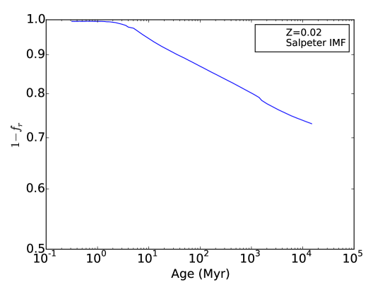
Figure 1: The mass evolution of a stellar population formed at same time with its age. The $f_{r}$ is “recycling fraction” factor.

To calculate $f_{r}(t-t^{\prime})$, we consider the mass evolution of an instantaneously formed stellar population using the FSPS code (Conroy & Gunn, 2010). This code can give the evolution of the current remained stellar mass fraction, which means $1-f_{r}$, of a simple stellar population after setting some necessary parameters. We choose the Salpeter IMF and solar metallicity while leaving other parameters as their default values in the code. Fig. 1 shows the evolution of the current mass fraction $1-f_{r}(t)$ of a simple stellar population. We can see that it has almost no mass loss within 1 Myr, then the fraction is up to about 0.27 at $14$ Gyr. If we just adopt a constant recycling fraction factor $R=0.27$, we will over-estimate the mass-loss effect in stellar evolution. The choice of IMF and metallicity will affect the evolution of $f_{r}$, which will be discussed in detail in discussion section.

Given the form of SFH $\psi(z)$, we can predict the SMH with equation (4) or equation (5). Both MD14 and G15 used equation (4), but their recycling fraction factors are slightly different, which are 0.27 and 0.28 respectively. In our work, we use the evolving $f_{r}$ instead of the constant one (hereafter, $f_{r}$ represents the evolving recycling factor while the $R$ represents the constant one). Since many previous works have been done to determine the evolution of cosmic SFH, we can use their results to predict the SMH with our $f_{r}$.

In the top panel of Fig. 2, the green and blue solid circles with $1\sigma$ errors are the observed SMD data given in MD14 and G15. The black solid line represents the SMH predicted from observed SFH in MD14 with $f_{r}$ while black dot-dashed line represents the one derived with $R=0.27$. The top panel of Fig. 3 is same as Fig. 2 but using the observed SFH in HB06. From these figures, we find that both instantaneous observed SFHs over-predict the SMH, and the SFH of MD14 gives a better prediction. Moreover, we also find that the $f_{r}$ gives different predictions comparing with a constant one especially at high redshifts. From the middle panels of these two figures, we can find that the SMHs predicted by observed SFHs with $f_{r}$ is little higher than those with $R$, and the larger factors are up to about $20\%$ at $z\sim 8$ in both cases.

We also use the MCMC method to derive the best-fitted SFH from the observed SMD data. We choose the SFH form as equation (2) used in MD14. And then we use equation (5) and MCMC method to fit the observed SMD data and obtain the optimal parameters. Our result is $(a,b,c,d)=(0.023,1.66,2.81,3.67)\pm(0.003,0.34,0.33,0.17)$, which is quite different from the best-fitting parameters $(a,b,c,d)=(0.015,2.7,2.9,5.6)$ obtained from observed SFR data given in MD14. In Fig. 2, the magenta solid line represents the SMH predicted from our best-fitting SFH from observed SMD data with SFH form in MD14 and the gray region shows the $95\%$ confidence region. We also use the SFH form in Cole et al. (2001), and obtain the optimal parameters $(a,b,c,d)=(0.030,0.058,2.361,2.707)$ $\pm$ (0.007,0.012,0.256,0.134) which is different with those of HB06. Cole et al. (2001) obtained optimal parameters as $(a,b,c,d)=(0.0166,0.1848,1.9474,2.6316)$ after considering the dust extinction. The SFH is much lower if there is not dust absorption and the optimal parameters are $(a,b,c,d)=(0.0,0.0798,1.658,3.105)$. The difference of these two case is about factor of three at $z\approx 2$. Our best-fitting SFH from observed SMD data lies between the SFHs of those two cases. Comparing with the predicted SMHs from best-fitting SFHs from observed SMD data, we find that the observed SFHs in both MD14 and HB06 over-predict the SMH. From the bottom panel of Figs. 2, we can find that the observed SFH from MD14 over-predicts the SMD by a factor of about two at the peak redshift about $z\sim 1.5$. The bottom panel of 3 shows that the observed SFH from HB06 over-predicts the SMD even by a factor of about four at the peak redshift about $z\sim 2$.

From Fig. 4, we find that the derived SFH from observed SMD data is much different from that given in MD14. Compared with the observed SFH of MD14, our best-fitting SFH is consistent with it at $z<0.5$ and $z>6$. But in the range $0.5<z<6$, our best-fitting SFH is lower. The lower factor peaks at about $z=2$ with about two. For the SFH form of Cole et al. (2001), Fig. 5 shows a similar result as Fig. 4. Wilkins et al. (2008) found that the observed SFH is consistent with the SFH inferred from SMD at $z<1$ but about 4 times larger at $z\approx 3$, which is different with ours. It may be caused by the different assumptions of IMF. Besides, Wilkins et al. (2008) only considered the SFH and SMD at $z<4$. We consider a large redshift range up to $z\sim 8$ and find that the SFH inferred from observed SMD data is consistent with observed SFH at $z>6$.

5 Discussion

In this work, we use a large observational data sample to test the discrepancy between the SMH and instantaneous SFH over the redshift range $0<z<8$. We find that there is a discrepancy between observed SMD and instantaneous SFH data. Just as said above, we choose a single power-law Salpeter IMF and solar metallicity in our analysis for simplicity. However, the estimations of SMD and SFRD depend on the assumptions of IMF and metallicity. Therefore we discuss the possible effect of the choice of IMF and metallicity on our result and some other potential causes for this discrepancy in this section.

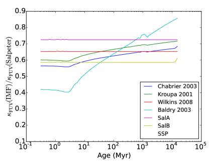
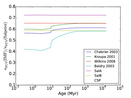
Figure 6: The ratio of mass-to-light from different IMFs to Salpeter IMF at FUV and IR bands. The top two panels is obtained from simple stellar populations, while the bottom two panels from complex stellar populations with a constant SFR.

Generally, the high-mass slope of IMF affects the estimation of SFRs since the young massive stars in a new born stellar population dominant the emission especially for the UV emission. While the low-mass slope of IMF affects the estimation of SMDs since the old low-mass stars dominant the stellar mass of a galaxy. Therefore, a more top-heavy IMF will generate more massive stars, which emit more radiation leading to a high luminosity-to-SFR ratio. Then we will obtain a low SFH for certain observed luminosity. Fig. 6 shows the converting factors of SFRD and SMD from traditional Salpeter IMF to different IMFs. The top two panels, which are obtained from simple stellar populations, show the converting factors of SFRDs in UV and IR luminosity respectively. The bottom two panels, which are obtained from complex stellar populations with a constant SFR, are for the SMDs. For the converting factors of SFRD, we choose the value in the first $1\rm\,Myr$. While for factors of SMD we use the value after $1\rm\,Gyr$ since the ratios become roughly unchanged in those time region. The rough converting factors are listed in Table 1. These converting factors are consistent with those given in previous literature (HB06, W08, MD14).

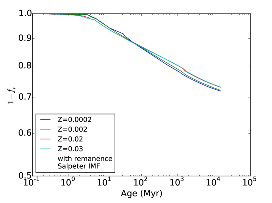
Figure 7: Top panel shows the dependence of $f_{r}$ on metallicity and the bottom one shows the dependence of $f_{r}$ on different IMFs.

What’s more, the choice of IMF can also affect the evolution of the recycling factor of a stellar population, since the stars with different initial mass have much different evolving processes and mass-loss rates. The top panel in Fig. 7 shows the dependence of the recycling factor on different IMFs. We find that, comparing with traditional Salpeter IMF, other IMFs with heavy massive end or light low-mass end give larger recycling factors, which can gives a lower predicted SMH from the observed SFH. The rough recycling factors of different IMFs are listed in Table 1. Considering the effects of the choice of different IMFs, the discrepancy between the observed SFRD and SMD will be relieved if we use the converting factors obtained with UV luminosity. For example, if we consider the observed SFH given in MD14 and the converting factor of UV luminosity, the IMFs of Chabrier (2003) and Kroupa (2001) will relieve the discrepancy at about $40\%$ level, while the IMF of Baldry & Glazebrook (2003) will relieve the discrepancy even at about $90\%$ level. The IMF of Baldry & Glazebrook (2003) can decrease the discrepancy at about $30\%$ level even using the converting factors obtained from IR luminosity.

Our current knowledge of the IMF remains remarkably poor (Kroupa, 2002). Some observations suggest that the actual IMF may deviate from the Salpeter IMF (Davé, 2008; van Dokkum, 2008). The redshift distribution of gamma-ray bursts can be explained by an evolving IMF (Wang & Dai, 2011). There are also some alternative IMFs such as Kroupa IMF Kroupa (2001) and Chabrier IMF Chabrier (2003). However some observations show that the IMF in local universe was not drastically different from Salpeter IMF over a wide range of environments (Weisz et al., 2015). So, more accurate and reliable observations and constraints on IMF are needed for the following study of the cosmic SFH and SMH.

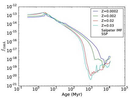
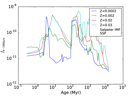
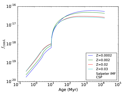
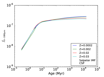
Figure 8: The dependence of UV and FIR luminosities on age and metallicity. The top two panels is obtained from simple stellar populations, while the bottom two panels from complex stellar populations with a constant SFR.

Except the IMF, the cosmic metallicity is also an important factor for the estimation of SFH and SMH. The systematic effect of the metallicity assumption needed to be discussed. We use the FSPS code of Conroy & Gunn (2010) to calculate the evolution of $f_{r}$ and the UV and IR luminosities of stellar populations under different metallicities. The top panel in Fig. 7 shows the dependence of $f_{r}$ on metallicity in Salpeter IMF. We can see that the dependence is not significant, since the $f_{r}$ only changes less than $3\%$ while the metallicity changes 100 times. The top two panels of Fig. 8 present the UV and IR luminosities of different metallicities under the Salpeter IMF for the simple stellar populations model. The bottom two panels for the complex stellar populations model. From those figures, we can see that the dependence of UV and IR luminosities on metallicity is significant since it will change $1.5-4$ times while the metallicity changing 100 times. Considering the observations of cosmic metallicity evolution, such as Rafelski et al. (2012) suggested the cosmic metallicity will less than $0.1\,Z_{\odot}$ at $z>2$, this result suggests that it would be better to take the effect of cosmic metallicity evolution into account in further analysis.

From Figs. 2 and 3 we can find that the observed SMD data are lower than the predicted value. Therefore, the SMD might be systematically underestimated. As we known that the mass of a galaxy is mainly dominated by its old low-mass stars but luminosity is dominated by young massive stars which will lead to the outshining problem. Maraston et al. (2010) studied the synthetic spectrum of a composite population formed with a constant SFR for $1~{}\rm{Gyr}$ and found the total spectrum was dominated by those stars formed in the latest $0.5\rm~{}Gyr$. The stellar mass of those galaxies with recent star formation will be systematically underestimated since the older stars are lost in the bright light of young stars. Therefore, we think that at the middle redshift range, like $1<z<3$, the SFR is so large that it will lead to a systematically underestimation of the SMDs since the outshining problem.

From Fig. 4 and Fig. 5 we can see that although the observed SMD data are lower than the SMD inferred from SFH at $z<0.5$. It doesn’t mean that the best-fitting SFH are also lower than the observed ones. In Fig. 4 and Fig. 5, the observed SFRs are much larger than the derived SFRs at middle redshift range $0.5<z<6$. The observed SFR is about two times as the derived one at $z\sim 2.0$. So the discrepancy between SMD and SFH can be also caused by an overestimation of SFRs, especially at middle redshift range $0.5<z<6$. Cole et al. (2001) found that the SFH would be much lower if there was not dust absorption. The difference of these two case is about factor of three at $z\approx 2$. Our best-fitting SFH from observed SMD data lies between the SFHs of those two cases. This hints that if we over-estimate the dust absorption effect, we will over-estimate the observed SFRDs.

6 Summary

In this article, we use a large observational data sample to test the discrepancy between the SMH and instantaneous SFH in the redshift range $0<z<8$. At first, we integrate the observed SFH over redshift to obtain the predicted SMH. We find that the inferred SMH is overpredicted at redshift $z<4$ especially for the observed SFH of H06. Although the SMH derived from the observed SFH of MD14 makes a much better comparison, it still has overpredicted problem with a factor of about two at redshift $z\sim 1.5$. Comparing with the results of the case using constant recycling factor $R$, the evolving $f_{r}$ will give $20\%$ less SMH at $z\sim 8$. Secondly, with the form of SFH in MD14, we use MCMC method to fit the observed SMD data and obtain the optimal parameters $(a,b,c,d)=(0.028,1.88,2.40,3.69)\pm(0.005,0.47,0.36,0.29)$, which are remarkably different with the result in MD14. The result is shown in Fig.2. Fig.4 shows the comparison between the derived SFH from observed SMD data and the observed SFRs. Comparing with the observed SFH of MD14, we can see that our best-fitting SFH is consistent with it at $z<0.5$ and $z>6$. But in the range of $0.5<z<6$, our best-fitting SFH is lower and even only half of observed one at about $z=2$. In order to remove the possible effect of the SFH form, we perform the same analysis with the form of SFH in Cole et al. (2001). For this SFH form, Fig. 5 shows a similar result as Fig. 4. Wilkins et al. (2008) found that the observed SFH is consistent with the SFH inferred from SMD at $z<1$ but about four times larger at $z\approx 3$, which is different with ours. Besides, Wilkins et al. (2008) only considered the SFH and SMD at $z<4$, but we consider a large redshift range up to $z\sim 8$ and find that the SFH inferred from observed SMD data is consistent with observed SFH at $z>6$.

We discuss some systematical effects of the assumptions of IMF and metallicity. A top-heavy or bottom light IMF can relieve the discrepancy between observed SFH and SMH. For example, if we consider the observed SFH given in MD14, the IMFs of Chabrier (2003), Kroupa (2001) and Baldry & Glazebrook (2003) will relieve the discrepancy at about $40\%$ to $90\%$ level, respectively. We find that metallicity doesn’t affect the evolution of recycling factor $f_{r}$ significantly, which is only about $3\%$ with 100 times change in metallicity. However, the metallicity affects the luminosities of UV and IR of stellar populations. We also discuss the effect of possible under-estimation of SMD and over-estimation of SFRD since the outshining problem and the possible over-estimation of dust extinction.

In order to solve the discrepancy between the observed SMH and SFH, we still need more accurate and reliable observations about the evolution of cosmic IMF and metallicity. The next generation of 30-meter ground-based telescopes or space telescopes are expected.

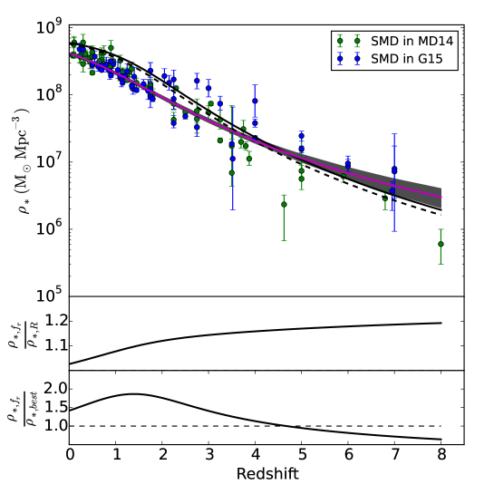
Figure 2: The redshift evolution of SMH. We use the SFH form of MD14 and their best-fitting parameters in this case. Top panel: the green and blue circles with $1\sigma$ errors are the observed SMD data given in MD14 and G15, respectively. The black solid line represents the SMH predicted from observed SFHs with an evolving factor $f_{r}$ and the black dot-dashed line represents the SMH predicted from observed SFHs with a constant factor $R$, respectively. The magenta line and the gray region are the inferred SMH from our best-fitting SFH from the observed SMD data and $95\%$ confidence region obtained with MCMC method. Middle panel: the ratio of the predicted SMHs from observed SFHs between evolving $f_{r}$ and constant $R$ at different redshift. It is up to about $1.2$ at $z=8$. Bottom panel: the ratio between SMHs from observed SFHs in MD14 and our best-fitting SFHs from observed SMD data with evolving $f_{r}$. It peaks at $z\sim 1.5$ with factor about 2.

Figure 3: Same as Fig. 2 but using the SFH form of Cole et al. (2001) and observed SFH given in HB06. In the bottom panel, the ratio peaks at $z\sim 2$ with factor about 4.

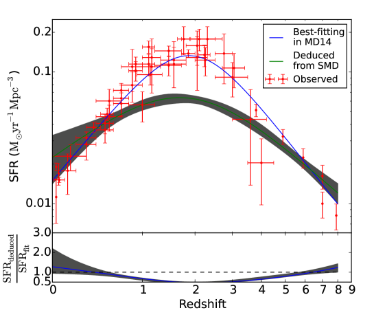
Figure 4: The SFH at $0<z<8$. Top panel: the red points with $1\sigma$ errors and the blue solid line are the observed SFR data and the best-fitting SFH given in MD14, respectively. The green solid line and gray region are our best-fitting SFH from observed SMD data and the $95\%$ confidence region obtained with MCMC method. The form of SFH using for MCMC fitting is given by MD14. Bottom panel: the ratio between our best-fitting SFH derived from observed SMD data and the best-fitting SFH in MD14.

Figure 5: Same as Fig. 4 but the SFH form of Cole et al. (2001) is used for MCMC fitting. It shows a similar result as the Fig. 4.

Table 1: The power-law slopes, recycling factors of different IMFs, and converting factors from Salpeter IMF to others IMFs.

IMF	Power-Law Slope (unit of mass: $M_{\odot}$)			$f_{r}^{a}$	Converting factor
	$0.08-0.5$	$0.5-1.0$	$1.0-100$		SFRDb	SMD
Salpeter	2.35	2.35	2.35	0.27	1	1
Chabrier	…c	…	-2.3	0.44	0.57 (0.59)	0.61 (0.58)
Kroupa	1.3	2.3	2.3	0.41	0.60 (0.63)	0.65 (0.62)
Wilkins	1.0	2.35	2.35	0.41	0.65	0.65
Baldry	1.5	2.15	2.15	0.47	0.42 (0.48)	0.58 (0.46)
SalA	1.5	2.35	2.35	0.37	0.73	0.73
SalB	1.5	1.5	2.35	0.46	0.59	0.59

^a The $f_{r}$ is measured at about 14 Gyr.

^b For those IMFs with two converting factors, the converting factor in brackets are obtained by comparing the IR luminosity and the other is from UV luminosity. For those IMFs with only one converting factor, it means the factors from UV and IR luminosities are same.

^c The IMF of Chabrier (2003) is $dn/dm\propto\exp{(-(\log{m}-\log{0.08})^{2}/(2\times 0.69^{2}))}/m$ for $m\leq 1\,M_{\odot}$.

Table 2: Stellar Mass Density Data.

Redshift Range	$\log(\rho_{z}^{*})\rm~{}[M_{\odot}~{}Mpc^{-3}]$	Reference
Data listed below are from Madau & Dickinson (2014) and
represented by green dots in Fig. 2 and 3
0.07	$8.59_{-0.01}^{+0.01}$	Li & White (2009)
0.005-0.22	$8.78_{-0.08}^{+0.07}$	Gallazzi et al. (2008)
0.0-0.2	$8.59_{-0.05}^{+0.05}$	Moustakas et al. (2013)
0.2-0.3	$8.56_{-0.09}^{+0.09}$
0.3-0.4	$8.59_{-0.06}^{+0.06}$
0.4-0.5	$8.55_{-0.08}^{+0.08}$
0.2-0.4	$8.46_{-0.12}^{+0.09}$	Bielby et al. (2012)
0.4-0.6	$8.33_{-0.03}^{+0.03}$
0.6-0.8	$8.45_{-0.10}^{+0.08}$
0.8-1.0	$8.42_{-0.06}^{+0.05}$
1.0-1.2	$8.25_{-0.04}^{+0.04}$
1.2-1.5	$8.14_{-0.06}^{+0.06}$
1.5-2.0	$8.16_{-0.03}^{+0.32}$
0.0-0.2	$8.75_{-0.12}^{+0.12}$	Pérez-González et al. (2008)
0.2-0.4	$8.61_{-0.06}^{+0.06}$
0.4-0.6	$8.57_{-0.04}^{+0.04}$
0.6-0.8	$8.52_{-0.05}^{+0.05}$
0.8-1.0	$8.44_{-0.05}^{+0.05}$
1.0-1.3	$8.35_{-0.05}^{+0.05}$
1.3-1.6	$8.18_{-0.07}^{+0.07}$
1.6-2.0	$8.02_{-0.07}^{+0.07}$
2.0-2.5	$7.87_{-0.09}^{+0.09}$
2.5-3.0	$7.76_{-0.18}^{+0.18}$
3.0-3.5	$7.63_{-0.14}^{+0.14}$
3.5-4.0	$7.49_{-0.13}^{+0.13}$
0.2-0.5	$8.55_{-0.09}^{+0.08}$	Ilbert et al. (2013)
0.5-0.8	$8.47_{-0.08}^{+0.08}$
0.8-1.1	$8.50_{-0.08}^{+0.08}$
1.1-1.5	$8.34_{-0.07}^{+0.10}$
1.5-2.0	$8.11_{-0.06}^{+0.05}$
2.0-2.5	$7.87_{-0.09}^{+0.09}$
2.5-3.0	$7.64_{-0.14}^{+0.15}$
3.0-4.0	$7.24_{-0.20}^{+0.18}$
0.2-0.5	$8.61_{-0.06}^{+0.06}$	Muzzin et al. (2013)
0.5-1.0	$8.46_{-0.03}^{+0.03}$
1.0-1.5	$8.22_{-0.03}^{+0.03}$
1.5-2.0	$7.99_{-0.03}^{+0.05}$
2.0-2.5	$7.63_{-0.04}^{+0.11}$
2.5-3.0	$7.52_{-0.09}^{+0.13}$
3.0-4.0	$6.84_{-0.20}^{+0.43}$
0.3	$8.78_{-0.16}^{+0.12}$	Arnouts et al. (2007)
0.5	$8.64_{-0.11}^{+0.09}$
0.7	$8.62_{-0.10}^{+0.08}$
0.9	$8.70_{-0.15}^{+0.11}$
1.1	$8.51_{-0.11}^{+0.08}$
1.35	$8.39_{-0.13}^{+0.10}$
1.75	$8.13_{-0.13}^{+0.10}$
0.1-0.35	8.58	Pozzetti et al. (2010)
0.35-0.55	8.49
0.55-0.75	8.50
0.75-1.00	8.42
0.5-1.0	8.63	Kajisawa et al. (2009)
1.0-1.5	8.30
1.5-2.5	8.04
2.5-3.5	7.74
1.3-2.0	$8.11_{-0.02}^{+0.02}$	Marchesini et al. (2009)
2.0-3.0	$7.75_{-0.04}^{+0.05}$
3.0-4.0	$7.47_{-0.13}^{+0.37}$
1.9-2.7	$8.10_{-0.03}^{+0.03}$	Reddy et al. (2012)
2.7-3.4	$7.87_{-0.03}^{+0.03}$
3.0-3.5	$7.32_{-0.02}^{+0.04}$	Caputi et al. (2011)
3.5-4.25	$7.05_{-0.10}^{+0.10}$
4.25-5.0	$6.37_{-0.54}^{+0.14}$
3.8	$7.24_{-0.06}^{+0.06}$	González et al. (2011)
5.0	$6.87_{-0.09}^{+0.08}$
5.9	$6.79_{-0.09}^{+0.09}$
6.8	$6.46_{-0.17}^{+0.14}$
3.7	$7.30_{-0.09}^{+0.07}$	Lee et al. (2012)
5.0	$6.75_{-0.16}^{+0.33}$
5.0	$7.19_{-0.35}^{+0.19}$	Yabe et al. (2009)
8.0	$5.78_{-0.30}^{+0.22}$	Labbé et al. (2013)
Data listed below are used in Grazian et al. (2015) and
represented by blue dots in Fig. 2 and 3
3.5-4.5	$7.36_{-0.03}^{+0.03}$	Grazian et al. (2015)
4.5-5.5	$7.20_{-0.06}^{+0.04}$
5.5-6.5	$6.94_{-0.10}^{+0.10}$
6.5-7.5	$6.90_{-0.44}^{+0.34}$
4.0	$7.58_{-0.06}^{+0.06}$	Duncan et al. (2014)
5.0	$7.39_{-0.07}^{+0.08}$
6.0	$6.98_{-0.11}^{+0.12}$
7.0	$6.86_{-0.56}^{+0.89}$
0.625	$8.42_{-0.08}^{+0.07}$	Tomczak et al. (2014)
0.875	$8.36_{-0.13}^{+0.13}$
1.125	$8.24_{-0.12}^{+0.12}$
1.375	$8.09_{-0.08}^{+0.08}$
1.75	$8.09_{-0.08}^{+0.08}$
2.25	$7.94_{-0.17}^{+0.16}$
0.6-1.0	$8.45_{-0.06}^{+0.06}$	Santini et al. (2012)
1.0-1.4	$8.28_{-0.08}^{+0.09}$
1.4-1.8	$8.16_{-0.07}^{+0.08}$
1.8-2.5	$8.18_{-0.11}^{+0.11}$
2.5-3.5	$8.10_{-0.13}^{+0.13}$
3.5-4.5	$7.91_{-0.24}^{+0.24}$
6.95	$6.57_{-0.14}^{+0.29}$	Labbé et al. (2010)
0.225	$8.68_{-0.09}^{+0.09}$	Pozzetti et al. (2007)
0.55	$8.57_{-0.08}^{+0.08}$
0.8	$8.45_{-0.11}^{+0.11}$
1.05	$8.37_{-0.12}^{+0.12}$
1.4	$8.27_{-0.14}^{+0.14}$
2.05	$8.28_{-0.11}^{+0.11}$
0.95	$8.46_{-0.07}^{+0.07}$	Dickinson et al. (2003)
1.70	$8.06_{-0.17}^{+0.13}$
2.25	$7.58_{-0.11}^{+0.07}$
2.75	$7.52_{-0.15}^{+0.14}$
0.3	$8.68_{-0.05}^{+0.06}$	Ilbert et al. (2010)
0.5	$8.44_{-0.04}^{+0.05}$
0.7	$8.44_{-0.03}^{+0.03}$
0.9	$8.50_{-0.03}^{+0.03}$
1.1	$8.28_{-0.04}^{+0.03}$
1.35	$8.13_{-0.03}^{+0.03}$
1.75	$7.97_{-0.24}^{+0.16}$
3.52	$7.05_{-0.77}^{+0.76}$	Marchesini et al. (2010)
1.25	$8.35_{-0.11}^{+0.10}$	Mortlock et al. (2011)
1.75	$8.36_{-0.12}^{+0.10}$
2.25	$8.23_{-0.14}^{+0.12}$
2.75	$8.21_{-0.11}^{+0.12}$
3.25	$7.87_{-0.11}^{+0.10}$
0.5	$8.46_{-0.03}^{+0.03}$	Fontana et al. (2006)
0.7	$8.37_{-0.02}^{+0.02}$
0.9	$8.29_{-0.03}^{+0.03}$
1.15	$8.18_{-0.02}^{+0.02}$
1.45	$8.07_{-0.03}^{+0.03}$
1.8	$7.94_{-0.04}^{+0.04}$
2.5	$7.68_{-0.04}^{+0.04}$
3.5	$7.27_{-0.02}^{+0.03}$

References

- Arnouts et al. (2007) Arnouts, S., Walcher, C. J., Le Fèvre, O., et al. 2007, A&A, 476, 137
- Baldry & Glazebrook (2003) Baldry, I. K., & Glazebrook, K. 2003, ApJ, 593, 258
- Bastian et al. (2010) Bastian, N., Covey, K. & Meyer, M. R., 2010, ARA&A, 48, 339
- Behroozi et al. (2013) Behroozi, P. S., Wechsler, R. H., & Conroy, C. 2013, ApJ, 770, 57
- Bernardi et al. (2013) Bernardi, M., Meert, A., Sheth, R. K., et al. 2013, MNRAS, 436, 697
- Bielby et al. (2012) Bielby, R., Hudelot, P., McCracken, H. J., et al. 2012, A&A, 545, A23
- Boquien et al. (2014) Boquien, M., Buat, V., & Perret, V. 2014, A&A, 571, A72
- Bouwens et al. (2012a) Bouwens, R. J., Illingworth, G. D., Oesch, P. A., et al. 2012a, ApJ, 754, 83
- Bouwens et al. (2012b) Bouwens, R. J., Illingworth, G. D., Oesch, P. A., et al. 2012b, ApJ, 752, L5
- Caputi et al. (2011) Caputi, K. I., Cirasuolo, M., Dunlop, J. S., et al. 2011, MNRAS, 413, 162
- Chabrier (2003) Chabrier, G. 2003, PASP, 115, 763
- Cole et al. (2001) Cole, S., Norberg, P., Baugh, C. M., et al. 2001, MNRAS, 326, 255
- Conroy & Gunn (2010) Conroy, C., & Gunn, J. E. 2010, ApJ, 712, 833
- Courteau et al. (2014) Courteau, S., Cappellari, M., de Jong, R. S., et al. 2014, Reviews of Modern Physics, 86, 47
- Dahlen et al. (2004) Dahlen, T., Strolger, L.-G., Riess, A. G., et al. 2004, ApJ, 613, 189
- Davé (2008) Davé, R. 2008, MNRAS, 385, 147
- Dickinson et al. (2003) Dickinson, M., Papovich, C., Ferguson, H. C., & Budavári, T. 2003, ApJ, 587, 25
- Draine & Li (2007) Draine, B. T., & Li, Aigen, 2007, ApJ, 657, 810
- Duncan et al. (2014) Duncan, K., Conselice, C. J., Mortlock, A., et al. 2014, MNRAS, 444, 2960
- Fioc & Rocca-Volmerange (1997) Fioc, M., & Rocca-Volmerange, B. 1997, A&A, 326, 950
- Fontana et al. (2004) Fontana, A., Pozzetti, L., Donnarumma, I., et al. 2004, A&A, 424, 23
- Fontana et al. (2006) Fontana, A., Salimbeni, S., Grazian, A., et al. 2006, A&A, 459, 745
- Gallazzi et al. (2008) Gallazzi, A., Brinchmann, J., Charlot, S., & White, S. D. M. 2008, MNRAS, 383, 1439
- González et al. (2011) González, V., Labbé, I., Bouwens, R. J., et al. 2011, ApJ, 735, L34
- Grazian et al. (2015) Grazian, A., Fontana, A., Santini, P., et al. 2015, A&A, 575, A96
- Gruppioni et al. (2013) Gruppioni, C., Pozzi, F., Rodighiero, G., et al. 2013, MNRAS, 432, 23
- Haardt & Madau (2012) Haardt, F., & Madau, P. 2012, ApJ, 746, 125
- Hopkins & Beacom (2006) Hopkins, A. M., & Beacom, J. F. 2006, ApJ, 651, 142
- Horiuchi et al. (2013) Horiuchi, S., Beacom, J. F., Bothwell, M. S., & Thompson, T. A. 2013, ApJ, 769, 113
- Ilbert et al. (2010) Ilbert, O., Salvato, M., Le Floc’h, E., et al. 2010, ApJ, 709, 644
- Ilbert et al. (2013) Ilbert, O., McCracken, H. J., Le Fèvre, O., et al. 2013, A&A, 556, A55
- Kajisawa et al. (2009) Kajisawa, M., Ichikawa, T., Tanaka, I., et al. 2009, ApJ, 702, 1393
- Kennicutt (1998) Kennicutt, R. C., Jr. 1998, ARA&A, 36, 189
- Kistler et al. (2009) Kistler, M. D., Yüksel, H., Beacom, J. F., Hopkins, A. M., & Wyithe, J. S. B. 2009, ApJ, 705, L104
- Kroupa (2001) Kroupa, P. 2001, MNRAS, 322, 231
- Kroupa (2002) Kroupa, P. 2002, Science, 295, 82
- Labbé et al. (2010) Labbé, I., González, V., Bouwens, R. J., et al. 2010, ApJ, 716, L103
- Labbé et al. (2013) Labbé, I., Oesch, P. A., Bouwens, R. J., et al. 2013, ApJ, 777, L19
- Lee et al. (2012) Lee, K.-S., Ferguson, H. C., Wiklind, T., et al. 2012, ApJ, 752, 66
- Li & White (2009) Li, C., & White, S. D. M. 2009, MNRAS, 398, 2177
- Li et al. (2011) Li, W., Chornock, R., Leaman, J., et al. 2011, MNRAS, 412, 1473
- Lonsdale Persson & Helou (1987) Lonsdale Persson, C. J., & Helou, G. 1987, ApJ, 314, 513
- Madau et al. (1998) Madau, P., Pozzetti, L., & Dickinson, M. 1998, ApJ, 498, 106
- Madau & Dickinson (2014) Madau, P., & Dickinson, M. 2014, ARA&A, 52, 415
- Magnelli et al. (2011) Magnelli, B., Elbaz, D., Chary, R. R., et al. 2011, A&A, 528, A35
- Magnelli et al. (2013) Magnelli, B., Popesso, P., Berta, S., et al. 2013, A&A, 553, A132
- Maraston et al. (2010) Maraston, C., Pforr, J., Renzini, A., et al. 2010, MNRAS, 407, 830
- Marchesini et al. (2009) Marchesini, D., van Dokkum, P. G., Förster Schreiber, N. M., et al. 2009, ApJ, 701, 1765
- Marchesini et al. (2010) Marchesini, D., Whitaker, K. E., Brammer, G., et al. 2010, ApJ, 725, 1277
- Mortlock et al. (2011) Mortlock, A., Conselice, C. J., Bluck, A. F. L., et al. 2011, MNRAS, 413, 2845
- Moustakas et al. (2013) Moustakas, J., Coil, A. L., Aird, J., et al. 2013, ApJ, 767, 50
- Muzzin et al. (2013) Muzzin, A., Marchesini, D., Stefanon, M., et al. 2013, ApJ, 777, 18
- Pérez-González et al. (2008) Pérez-González, P. G., Rieke, G. H., Villar, V., et al. 2008, ApJ, 675, 234
- Pozzetti et al. (2007) Pozzetti, L., Bolzonella, M., Lamareille, F., et al. 2007, A&A, 474, 443
- Pozzetti et al. (2010) Pozzetti, L., Bolzonella, M., Zucca, E., et al. 2010, A&A, 523, A13
- Rafelski et al. (2012) Rafelski, M., Wolfe, A. M., Prochaska, J. X., Neeleman, M., & Mendez, A. J. 2012, ApJ, 755, 89
- Reddy & Steidel (2009) Reddy, N. A., & Steidel, C. C. 2009, ApJ, 692, 778
- Reddy (2011) Reddy, N. A. 2011, UP2010: Have Observations Revealed a Variable Upper End of the Initial Mass Function?, 440, 385
- Reddy et al. (2012) Reddy, N., Dickinson, M., Elbaz, D., et al. 2012, ApJ, 744, 154
- Renzini & Voli (1981) Renzini, A., & Voli, M. 1981, A&A, 94, 175
- Salim et al. (2007) Salim, S., Rich, R. M., Charlot, S., et al. 2007, ApJS, 173, 267
- Salpeter (1955) Salpeter, E. E. 1955, ApJ, 121, 161
- Santini et al. (2012) Santini, P., Fontana, A., Grazian, A., et al. 2012, A&A, 538, A33
- Santini et al. (2015) Santini, P., Ferguson, H. C., Fontana, A., et al. 2015, ApJ, 801, 97
- Schenker et al. (2013) Schenker, M. A., Robertson, B. E., Ellis, R. S., et al. 2013, ApJ, 768, 196
- Tomczak et al. (2014) Tomczak, A. R., Quadri, R. F., Tran, K.-V. H., et al. 2014, ApJ, 783, 85
- Utomo et al. (2014) Utomo, D., Kriek, M., Labbé, I., Conroy, C., & Fumagalli, M. 2014, ApJ, 783, L30
- van Dokkum (2008) van Dokkum, P. G. 2008, ApJ, 674, 29
- Wanderman & Piran (2010) Wanderman, D., & Piran, T. 2010, MNRAS, 406, 1944
- Wang & Dai (2009) Wang, F. Y., & Dai, Z. G. 2009, MNRAS, 400, L10
- Wang & Dai (2011) Wang, F. Y., & Dai, Z. G. 2011, ApJ, 727, 34
- Weisz et al. (2015) Weisz, D. R., et al., 2015, ApJ, 806, 198
- Wilkins et al. (2008) Wilkins, S. M., Trentham, N., & Hopkins, A. M. 2008, MNRAS, 385, 687
- Woosley & Weaver (1995) Woosley, S. E., & Weaver, T. A. 1995, ApJS, 101, 181
- Yabe et al. (2009) Yabe, K., Ohta, K., Iwata, I., et al. 2009, ApJ, 693, 507