The dust environment of comet 67P/Churyumov-Gerasimenko from Rosetta OSIRIS and VLT observations in the 4.5 to 2.9 au heliocentric distance range inbound

Abstract

Context. The ESA Rosetta spacecraft, currently orbiting around comet 67P, has already provided in situ measurements of the dust grain properties from several instruments, particularly OSIRIS and GIADA. We propose adding value to those measurements by combining them with ground-based observations of the dust tail to monitor the overall, time-dependent dust-production rate and size distribution.

Aims. To constrain the dust grain properties, we take Rosetta OSIRIS and GIADA results into account, and combine OSIRIS data during the approach phase (from late April to early June 2014) with a large data set of ground-based images that were acquired with the ESO Very Large Telescope (VLT) from February to November 2014.

Methods. A Monte Carlo dust tail code, which has already been used to characterise the dust environments of several comets and active asteroids, has been applied to retrieve the dust parameters. Key properties of the grains (density, velocity, and size distribution) were obtained from Rosetta observations: these parameters were used as input of the code to considerably reduce the number of free parameters. In this way, the overall dust mass-loss rate and its dependence on the heliocentric distance could be obtained accurately.

Results. The dust parameters derived from the inner coma measurements by OSIRIS and GIADA and from distant imaging using VLT data are consistent, except for the power index of the size-distribution function, which is $\alpha$=–3, instead of $\alpha$=–2, for grains smaller than 1 mm. This is possibly linked to the presence of fluffy aggregates in the coma. The onset of cometary activity occurs at approximately 4.3 au, with a dust production rate of 0.5 kg/s, increasing up to 15 kg/s at 2.9 au. This implies a dust-to-gas mass ratio varying between 3.8 and 6.5 for the best-fit model when combined with water-production rates from the MIRO experiment.

1 Introduction

Figure 1: OSIRIS NAC images used in this work. All the images are oriented North up and East to the left. The lower labels in each image indicates the observation date. All images are 30$\times$35 pixels. Their spatial dimensions at the comet can be calculated using the spatial resolution indicated in the last column of Table 1. The straight features near the diagonals in the uppermost first and third panels from the left are artifacts.

Comets are among the least processed objects in the solar system, which means that their study provides insights into their origin and evolution. The Grain Impact and Dust Accumulator (GIADA) (Colangeli et al., 2009; Della Corte et al., 2014) and the Optical, Spectroscopic, and Infrared Remote Imaging System (OSIRIS) (Keller et al., 2007) on board the ESA Rosetta spacecraft have been in operation in the vicinity of comet 67P/Churyumov-Gerasimenko (hereafter 67P) since March 2014. The OSIRIS camera started to provide images of the comet since March 23, 2014 (Sierks et al., 2015; Tubiana et al., 2015a), while the first measurements carried out by GIADA were performed on July 18, 2014, when the comet was at heliocentric distances of 4.3 au and 3.7 au, respectively.

Combining these OSIRIS and GIADA early single grain measurements, Rotundi et al. (2015) derived the dust environment in the 3.7-3.4 au range, which agrees with model predictions by Fulle et al. (2010) at 3.2 au. Thus, the particle differential size distribution was found to be adequately described by a differential power law of index $\alpha$=–2, except for the largest particle size bins ($r\gtrsim$1 mm) for which an index $\alpha$=–4 is needed to satisfy the 67P trail data, which are mostly sensitive to those large particles, and which were acquired in previous revolutions (Agarwal et al., 2010). A close value of $\alpha\sim$–3.7 for large particles has been found by Soja et al. (2015) from analysis of 67P trail Spitzer data. This also agrees with the distribution of blocks that are larger than a few centimetres in size on the surface of smooth terrains found by Mottola et al. (2015) ($\alpha$=–3.8$\pm$0.2) from the Rosetta Lander Imaging System (ROLIS) on board Philae. This is also in line with the steep distribution of large particles found by Kelley et al. (2013a) in comet 103P/Hartley 2 coma ($\alpha$=–4.7). The maximum grain size ejected that was reported by Rotundi et al. (2015) was 2 cm, and a dust loss rate of 7$\pm$1 kg s^-1 was determined, giving a dust-to-gas mass ratio (d/g) of 4$\pm$2 when combined with water production-rate data from the Microwave Instrument for the Rosetta Orbiter (MIRO) (Gulkis et al., 2015). Assuming spherical particles, a grain density of 1900$\pm$1100 kg m^-3 was derived. Interestingly, the velocity of outflowing grains did not show any link with particle size. Hydrodynamic models of the inner coma (e.g. Crifo et al., 2004) would be needed to explain such behavior.

Recently, a detailed study of GIADA data in the 3.4-2.3 AU heliocentric distance range has been performed by Della Corte et al. (2015). In this study, two populations of grains, both compact and fluffy, are described in relation to the geographical location of emission. Using the same GIADA data, the contribution of the fluffy grain component to the brightness of the coma has been found as being less than 15% by Fulle et al. (2015a). These fluffy grains have also been collected with the Cometary Secondary Ion Mass Analyser (COSIMA) on board Rosetta, which shows no trace of ice in their composition beyond 3 au (Schulz et al., 2015).

In contrast with the random distribution of velocities versus grain size found by Rotundi et al. (2015), the relation of emission velocities and particle mass ($m$) found by Della Corte et al. (2015) was quite steep, albeit with a 50% uncertainty, given by a power law $v\propto m^{\gamma_{m}}$ with $\gamma_{m}$=–0.32$\pm$0.18, which translates to $v\propto r^{\gamma_{r}}$ as $\gamma_{r}$=–0.96$\pm$0.54 ($r$ is particle radius). This is still compatible with the widely used $v\propto r^{-0.5}$ dependence that is based on simple hydrodynamical considerations (Whipple, 1950). Photometric measurements of individual grains at 2.25 AU and 2.0 AU from OSIRIS images suggest a $v\propto r^{-0.5}$ dependence (Fulle et al., 2015b). The different dependencies of particle velocity from the particle radius determined by Rotundi et al. (2015) and Della Corte et al. (2015) might be related to the various nucleus heliocentric distances and/or different spacecraft-nucleus distances involved. Only detailed hydrodynamic calculations in the inner coma, including the detailed nucleus shape, will allow a proper interpretation of those data. Consequently, the model runs with the different particle-velocity distributions since inputs are needed to determine which distribution is the most compatible with our observations.

Figure 2: High signal-to-noise WAC image obtained as a median stack of 117 frames, obtained on May 17 and 18 2014. The dimensions of the image are 3690$\times$3690 km at the nucleus distance. The innermost isophote level corresponds to 2.24$\times$10^-8 W m^-2 sr^-1 nm^-1, decreasing outwards in factors of 2. North is up, East to the left.

In this paper, we combine OSIRIS images acquired between April and July 2014 with ground-based images taken with the FOcal Reducer and low dispersion Spectrograph 2 (FORS2) at the ESO VLT between February and November 2014, when the comet was observable from the southern hemisphere. From late November 2014 to late May 2015, the comet was behind the Sun for ground observers. The comet 67P could be observed again from late May 2015 from the southern hemisphere and from July 2015 from the northern hemisphere. Ground-based observations, combined with the simultaneous OSIRIS data described above, provide a unique opportunity to determine the dust properties and their time evolution because they are most sensitive to the large-scale tail structure that cannot be mapped from the spacecraft. Processes such as significant volatile loss or grain fragmentation that take place a few days after ejection cannot be monitored by OSIRIS.

Figure 3: Subset of 20 out of the 52 VLT/FORS2 images taken between February and November 2014, with the R-SPECIAL filter. North is up, East to the left in all images. The date of observation is indicated in each panel. All the images have 40$\times$40 pixels in size, which can be converted to physical size at the comet using the spatial resolution values of last column of Table A.1 (see Appendix A).

2 The Observations

We used two data sets:

• OSIRIS Narrow Angle Camera (NAC) and Wide Angle Camera (WAC) images obtained from late April to early July 2014.

• VLT/FORS2 images obtained from mid-February to late November 2014.

A description of the instrumentation and the data reduction follows.

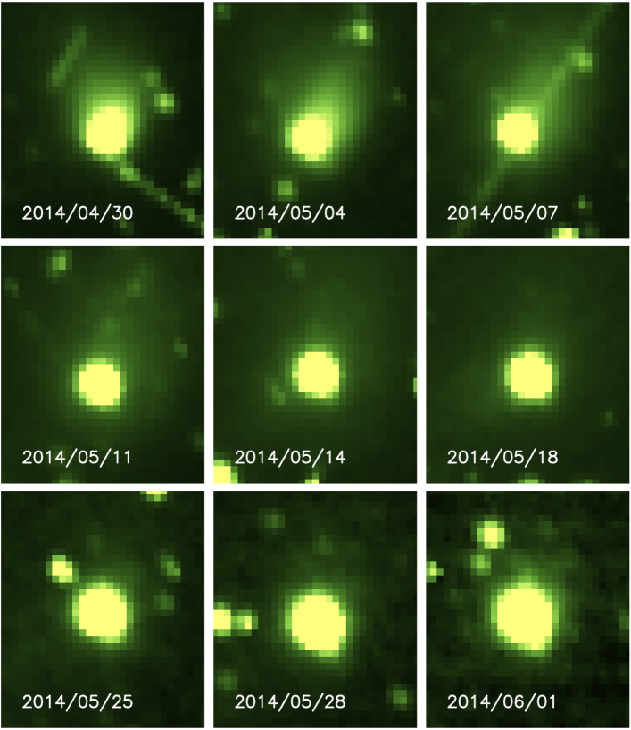
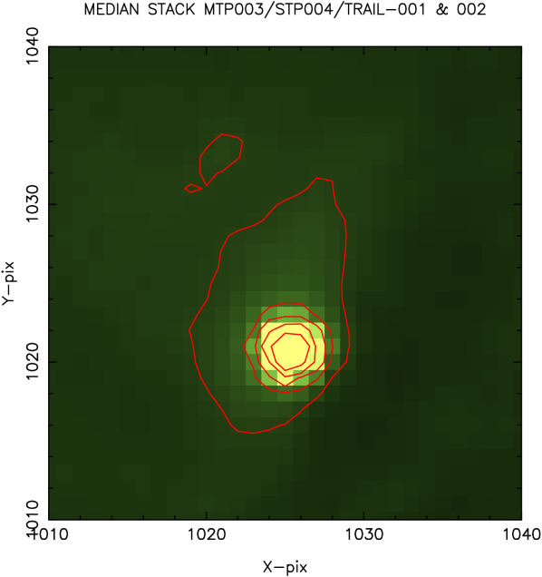
The OSIRIS instrument (Keller et al., 2007) comprises two cameras, the NAC, with a field of view (FOV) of 2.20${}^{\circ}\times$2.22^∘ and an angular resolution of 1.87$\times$10^-5 rad px^-1, and the WAC, with a FOV of 11.35${}^{\circ}\times$12.11^∘ with an angular resolution of 1.01$\times$10^-4 rad px^-1. We used NAC images taken with the Orange filter, which has a central wavelength of 649.2 nm, and a bandwidth of 84.5 nm. The WAC images used were taken with the Red filter, which has a central wavelength of 629.8 nm and a bandwidth of 158.6 nm. In both cases, we used Level 3 images, which were processed following the standard OSIRIS calibration pipeline, including bias subtraction, flat-fielding, distortion correction, and radiometric calibration (Tubiana et al., 2015b). The log of the nine NAC observations is given in Table 1, and Fig. 1 displays the NAC images. The WAC observations consisted of a sequence of 117 images acquired between 2014-05-17T07:59:16 and 2014-05-18T06:52:05 (UT), and were aimed at the detection of a trail feature. For the dust-tail modeling, we combined all 117 frames into a single median stack, resulting in a high signal-to-noise image (see Fig 2). The spatial resolution of this image is 123 km px^-1.

Table 1: Observational circumstances for the OSIRIS NAC observations

Date	r	S/C-Comet	Phase angle	Position angle	Resolution
(UT)	(AU)	distance (AU)	(deg)	(deg)	(km px-1)
2014-04-30T06.25.55.567	4.111	0.01586	35.10	120.697	44.410
2014-05-04T03.17.55.567	4.093	0.01412	35.28	120.444	39.557
2014-05-07T03.17.56.528	4.078	0.01278	35.40	120.234	35.796
2014-05-11T12.49.46.645	4.057	0.01086	35.53	119.902	30.410
2014-05-14T12.37.30.576	4.042	0.00956	35.56	119.647	26.760
2014-05-18T12.21.10.575	4.023	0.00782	35.50	119.239	21.896
2014-05-25T11.51.14.558	3.988	0.00540	35.32	118.497	15.131
2014-05-28T11.38.14.574	3.973	0.00460	35.26	118.202	12.891
2014-06-01T11.20.54.559	3.953	0.00354	34.95	117.682	9.907

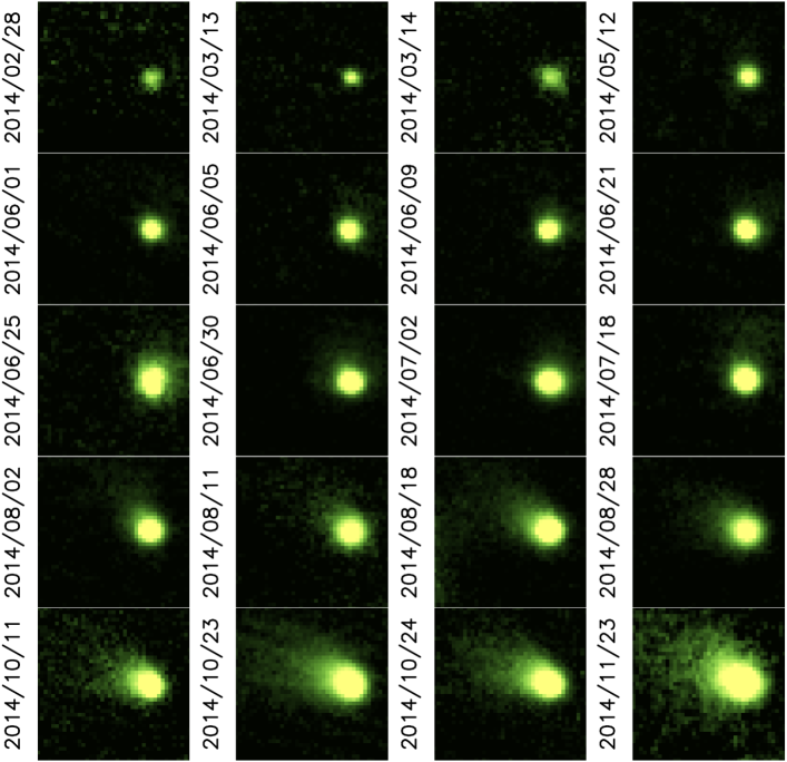
The VLT data consist of CCD images acquired with the R-SPECIAL filter (spectral response close to that of Bessell R, with central wavelength of 655 nm and bandwidth of 165 nm). FORS was used in imaging mode with the standard resolution collimator, and the detector was read binning 2$\times$2, which resulted in an image scale of 0.25$\arcsec$ px^-1. The reduction of the images was performed using standard techniques, encompassing bias and flat-fielding, and photometric calibration by standard star field imaging. In addition to the standard techniques, the images were also processed with a background subtraction algorithm to remove the crowded star fields (Bramich, 2008). For each night of observation, a median stack of the available images was produced and the magnitude within an aperture of 10 000 km radius was measured. Full details on the data set and the reduction procedure are given by Snodgrass et al. (2015).

The log of the observations is given in Table A.1 (see Appendix A), and a subset of the VLT images is displayed in Fig. 3. The images were converted from mag arcsec^-2 ($m$) to mean solar disk intensity units ($i/i_{0}$), according to the relationship

$$m=2.5\log\Omega+m_{\sun}-2.5\log(i/i_{0}),$$ (1)

where $\Omega$ is the solid angle of the Sun at 1 au (2.893$\times$10⁶ arcsec²), and $m_{\sun}$ is the magnitude of the Sun in the Bessell R filter ($m_{\sun}$=–27.09).

We emphasise the importance of the different viewing angles and spatial scales of the OSIRIS and VLT image sets. While for the OSIRIS images the resolution ranges from 44 to 10 km px^-1, the VLT images provide a spatial resolution from nearly 900 km px^-1 to $\sim$490 km px^-1 at the closest geocentric distance of 2.7 au.

An important aspect of the observations is the nucleus brightness contribution to the images. Since the OSIRIS images and the early VLT images were acquired at large heliocentric distances when the comet was displaying little activity, the nucleus signal to the image brightness dominates over the coma brightness and this must be taken into account. The total observed brightness of the images can be expressed as a sum of the nucleus plus the coma brightness contributions convolved with the corresponding point spread function (PSF) as (e.g. Lamy et al., 2006)

$$B(x,y)=[C(x,y)+N(x,y)]\otimes P(x,y),$$ (2)

where $C(x,y)$, $N(x,y)$, and $P(x,y)$ are the coma, nucleus, and PSF as functions of the pixel coordinates of the image relative to the nucleus position, identified by the brightest pixel in the images.

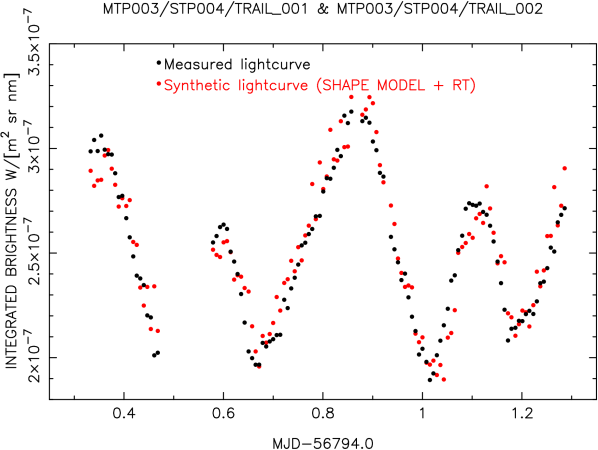
To calculate the nucleus brightness at each epoch, we developed a photon ray-tracing algorithm from which we constructed synthetic images of the nucleus as it would be seen either from the spacecraft or from the Earth. We used an early shape model of the nucleus (SHAP4S) (Preusker et al., 2015) with a rotational axis pointing to RA=69.54^∘, DEC=64.11^∘ (J2000 coordinates), a Lambertian surface model with a certain albedo value (the same for all the red filters used), a linear phase coefficient of 0.047 mag deg^-1 (Fornasier et al., 2015), and a rotational period of 12.4043h, the appropriate value at the time of the observation (Mottola et al., 2014). The albedo value was constrained by matching a synthetic lightcurve to the experimental lightcurve derived from the sequence of WAC images obtained on May 17 and 18 2014, as described. The resulting albedo is 0.06, which is close to the peak value of 0.063 obtained by Fornasier et al. (2015) from the derived gaussian distribution of surface albedos.

Although a noticeable coma is present in the images, its coma contribution to the integrated nucleus plus coma system brightness at such heliocentric distances ($\sim$4 AU) is negligible, being estimated to be below the relative photometric error of the measurements (Mottola et al., 2014). This contribution can be evaluated from the model results that are described in the next sections. The integrated brightness for the WAC image of Fig. 2 is 2.79$\times$10^-7 W m^-2 sr^-1 nm^-1. For our best-fit Model 1, which is characterised by a power-law particle-size distribution with power index of –3 and a random distribution of particle ejection velocities (see Sects. 3 and 4 for a detailed description of the model), we obtain 2.84$\times$10^-7 W m^-2 sr^-1 nm^-1 for the nucleus+coma system, which is in close agreement with the measured brightness. From the same model, the integrated signal of the coma alone is just 1.30$\times$10^-11 W m^-2 sr^-1 nm^-1, i.e. less than 0.005% of the total signal. Thus, the coma contribution can be safely ignored for the construction of the nucleus lightcurve from the images at such heliocentric distances. To obtain the integrated brightness at each observation date, an aperture radius equal to the full width at half maximum (FWHM) of the field stars was used. Fig. 4 shows a comparison of the measured lightcurve and the one calculating the integrated brightness from the synthetic nucleus images, assuming a surface albedo of 0.06, as previously mentioned. Along the lightcurve, the mean value of the difference between measured and computed nucleus brightness is 1%, while the maximum difference is 16%. These discrepancies are most likely related to the simplicity of the surface model and to local variations of surface albedo (Fornasier et al., 2015).

The coma/tail brightness distribution is computed with the Monte Carlo dust tail code. This is described in the next section.

Figure 4: Lightcurve obtained from the analysis of 117 frames from WAC Red filter images obtained on 2014 May 17 and 18 (black dots). The red dots correspond to a simulation of the lightcurve, taking in consideration a nucleus shape model (Preusker et al., 2015) with a Lambertian model for the surface, which has an albedo of 0.06, and a ray-tracing technique to compute the total output flux at the S/C position.

3 The model

The Monte Carlo dust tail code has been described previously (e.g. Fulle et al., 2010; Moreno et al., 2012). Briefly, this is a forward model that, given all the dust input parameters, computes synthetic dust tail images for a given date by the trial-and-error procedure. To this end, the code computes the trajectory of a large number of spherical particles that are ejected from a small-sized nucleus, assuming that the grains are affected by the solar gravitation and the solar radiation pressure. The nucleus gravitational field is neglected at distances where the gas drag vanishes (at approximately 20 nuclear radii, R_N). Under these assumptions, the trajectory of the particles is Keplerian and the orbital elements are computed from the assumed terminal velocities (at 20R_N). The $1-\mu$ parameter (e.g. Fulle, 1989), which is the ratio of solar radiation pressure force to solar gravity force, is given by $1-\mu=C_{pr}Q_{pr}/(2\rho r)$. In this equation, $C_{pr}$ is given by

$$C_{pr}=\frac{3E_{s}}{8\pi cGM_{\sun}}=1.19\times 10^{-3}\text{kg m${}^{-2}$},$$ (3)

where $E_{s}$ is the mean total solar radiation, $c$ is the speed of light, $G$ is the universal gravitational constant, and $M_{\sun}$ is the solar mass (Finson & Probstein, 1968). $Q_{pr}$ is the radiation pressure coefficient, and $\rho$ is the particle density. The radiation pressure coefficient for absorbing particles with radii $r\gtrsim$1 $\mu$m is $Q_{pr}\sim$1 (e.g. Moreno et al., 2012). The geometric albedo of the particles at red wavelengths is assumed to be $p_{v}$=0.065, a value close to to the one that was determined for the geometric albedo of the nucleus, and which ranged from 0.0589 to 0.072 at 535 and 700 nm, respectively, from disk-averaged photometry using OSIRIS NAC data (Fornasier et al., 2015). For the dust particles, we assumed a phase angle coefficient of 0.03 mag deg^-1 in agreement with the value reported by Snodgrass et al. (2013) for comet 67P, and within the range estimated for other comets (e.g. Meech & Jewitt, 1987). In addition to the input model parameters just described, we need to set the size-distribution function and the dust-loss rate, as a function of the heliocentric distance.

In most previous applications of the code, the dust tail code was applied with almost no previous knowledge of any of the dust properties. However, the observations of the inner coma dust grains by OSIRIS and GIADA provide a unique characterisation of fundamental dust parameters as described in Sect. 1. We used the dust physical parameters described by Rotundi et al. (2015) as inputs for the Monte Carlo code: the particle-size distribution is governed by a power law with index –2 (except at sizes larger than 1 mm, for which the index is –4), the largest particles ejected are 1 cm in radius, and the particle density is set to 2000 kg m^-3. Taking into account the distributions of particle velocities found by Rotundi et al. (2015) and Della Corte et al. (2015), we have devised three different models with distinct grain-velocity dependencies, all of the form $v(\mu,t)=v_{1}(\mu)u(t)$, $v_{1}(\mu)$ being a size-dependent velocity function, and $u(t)$ a dimensionless time-dependent parameter. These models range from a velocity that is independent of particle size, as found by Rotundi et al. (2015), to a steep function of velocity on grain size, as derived in Della Corte et al. (2015). Specifically, in Model 1, the terminal velocity of the grains is given by $v(\mu,t)=rnd[1,5]u(t)$, where $rnd[1,5]$ is a random value in the 1 to 5 m s^-1 interval; in Model 2, the terminal velocity is given by $v(\mu,t)=1320(1-\mu)^{0.96}u(t)$ m s^-1; and in Model 3, we set $v(\mu,t)=45(1-\mu)^{0.42}u(t)$ m s^-1, in agreement with the most probable value, and the lower limit in the power-law exponent of the velocity versus particle size as determined by Della Corte et al. (2015), respectively. We note that these functions are, in all cases, derived for a certain range of particle radii only, within the range of instrumental sensitivity, mostly in the 0.1 to 10 mm domain. Fig. 5 displays the just described size-dependent term of the terminal velocities for each model and Fig. 6 shows the time-dependent component $u(t)$.

Figure 5: Size-dependent component of the terminal velocity of the dust grains assumed in the Monte Carlo model. Model 1 corresponds to the random velocity distribution found by Rotundi et al. (2015), Model 2 corresponds to the steep, most probable value, $v\propto r^{-0.96}$ found by Della Corte et al. (2015), and Model 3 to the less steep dependence given by $v\propto r^{-0.42}$. The escape velocity at 20R_N is also indicated.

Figure 6: Assumed time-dependent component of the terminal velocity of the dust grains assumed in the Monte Carlo model. The bump between –4.25 to –4.15 AU is related to the 30 April 2014 outburst.

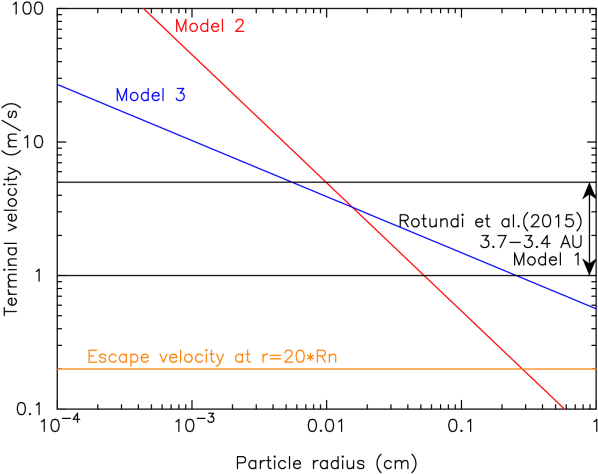
The function $u(t)$ reflects the overall time-dependence of the velocity and is constrained as $u(t)=1$ in the heliocentric distance range 3.7-3.4 au from the results of Rotundi et al. (2015) for Model 1. Out of this heliocentric distance range, and for Models 2 and 3, a free parameter is adjusted by the trial and error procedure, taking into account that it should increase after the onset of activity (e.g. Fulle et al., 2010), and it is further enhanced whenever an outburst occurs, as has been observed, e.g. after the 2007 outburst of comet 17P/Holmes (Montalto et al., 2008; Moreno et al., 2008). The other free parameters that must be set are the dust-loss rate as a function of the heliocentric distance, and the activation time. The heliocentric dependence of the dust-mass loss rate is initially assumed as a function that varies as the inverse square of the heliocentric distance, and then several tens of test functions that modify the initial profile are introduced until a good fit to all the datasets of OSIRIS and VLT images is reached. Thus, the presence of outbursts, such as that of 30 April 2014 (Tubiana et al., 2015a) imply a sudden increase of the dust-loss rate that clearly has to be taken into account to fit the data. The goodness of the fit for each model is characterized by the quantity

$$\chi^{2}=\left|\sum_{i,j}\frac{\left[\log(I_{obs}(i,j))-\log(I_{mod}(i,j))\right]^{2}}{\log(I_{mod}(i,j))}\right|,$$ (4)

where $I_{obs}$ and $I_{mod}$ are the observed and modeled brightness, and the summation is extended to the pixels $(i,j)$ along a scan in the anti-solar direction (position angle of the Sun-to-comet radius vector), passing through the brightest pixel. This $\chi^{2}$ parameter is calculated for each image, and then the total summation of the $\chi^{2}$ for all the OSIRIS plus VLT images is the parameter used as the quality of the fit for each model. As previously stated, the size distribution is initially set to a power law of index –2 and the maximum particle radius to 1 cm, in accordance with Rotundi et al. (2015). The minimum particle radius is set initially to 1 $\mu$m, but tests will also be made for smaller and larger minimum size, as described below.

Another input parameter of the model is the emission pattern. The OSIRIS images acquired in August 2014 when Rosetta was at a distance from the comet, when the nucleus shape could be clearly resolved (Sierks et al., 2015; Lara et al., 2015), revealed a number of conspicuous jets coming from the neck region (Hapi) and pointing towards the direction of the pole. In our model, we imposed a relatively higher number of particles launched from latitudes higher than 60^∘ than from elsewhere. Specifically, we set 35% of particles (in number) as being emitted from that region and 65% from latitudes south of 60^∘. This corresponds to a flux of particles that are 7.5 times higher at those high latitudes than elsewhere. To keep the number of free parameters to a minimum, we have not attempted to modify the emission pattern along the orbital arc. This highly anisotropic ejection pattern, with particle emission directed to the north, has already been inferred by Fulle et al. (2010) in the GIADA dust environment model from model fits to 67P data that was acquired during three revolutions around the Sun prior to the Rosetta encounter.

4 Results and discussion

Once a set of model parameters has been defined, we run the Monte Carlo dust tail code for all the OSIRIS and VLT images involved in the analysis. However, for clarity, and to save space, we will only show the results for subsets of them. Specifically, four dates are selected for the OSIRIS images, and twenty for the VLT images. In each case, the isophotes will be shown in the same brightness units of W m^-2 sr^-1 nm^-1 (as for the Level 3 OSIRIS images), and in units of the solar disk intensity for the VLT images.

Figure 7: Monte Carlo dust tail code simulations (red contours) compared to the OSIRIS NAC observations (black contours) for the input parameters derived from Rotundi et al. (2015) with a power-law exponent of the size distribution function of –2. The innermost isophotes have a value of 3.2$\times$10^-8 W m^-2 sr^-1 nm^-1 in all four images and decrease in factors of 2 outwards.

Figure 8: Monte Carlo dust tail code simulations (red contours) compared to the VLT observations (black contours) for the input parameters derived from Rotundi et al. (2015) with a power-law exponent of the size distribution function of –2. The image dates are shown on the left side of each panel. Innermost isophotes are 4$\times$10^-12 solar disk units, except for panels 2014/02/28 and 2014/03/14, which have 2$\times$10^-12 solar disk units.

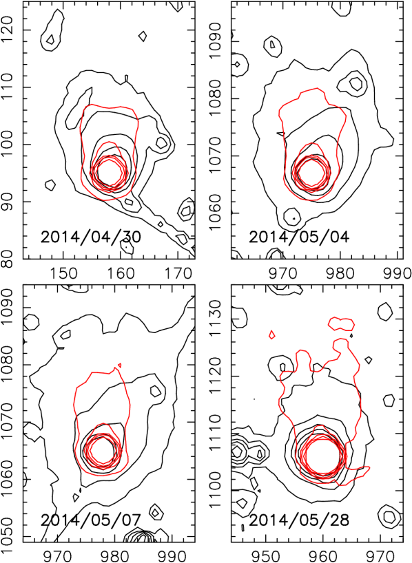
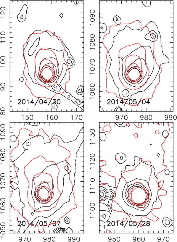
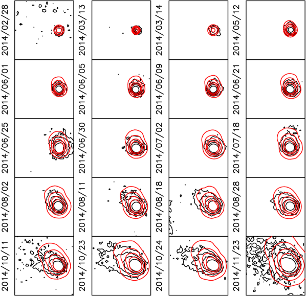
We start by displaying the results of Model 1, the one which has a random distribution of terminal particle velocities as described above. For this model, we obtain the results shown in Figs. 7 and 8 for the OSIRIS NAC and VLT images, respectively, corresponding to the best-fit dust-mass loss rate displayed in Fig. 9. This graph shows a peak at about 4.11 au pre-perihelion that corresponds to the outburst that occurred on 30 April 2014, in which a total dust-loss mass of $\sim$7$\times$10⁶ kg was released. The comet shows some activity, at the level of $\sim$0.5 kg s^-1, already at 4.3 au pre-perihelion. This is in agreement with the findings of Snodgrass et al. (2013) for the previous orbit and their predictions for the current orbit. In their trail model, Soja et al. (2015) reported values of $\sim$10 kg s^-1 at 3 au, which is in line with ours, but of $\sim$3.5 kg s^-1 at 4.3 au, a value that is considerably larger than our estimate at that heliocentric distance.

Figure 9: Best-fit dust-mass loss rate as a function of the heliocentric distance for power-law size distributions of –2 (solid line) and –3 (dotted line). Note the increase in mass loss rate at the time of the 30 April 2014 outburst.

Figure 10: Monte Carlo dust tail code simulations (red contours) compared to the OSIRIS NAC observations (black contours) for the input parameters derived from Rotundi et al. (2015) with a power-law exponent of the size distribution function of –3 and the random distribution of terminal velocities (Model 1).

Figure 11: Monte Carlo dust tail code simulations (red contours) compared to the VLT observations (black contours), for the input parameters derived from Rotundi et al. (2015), with a power-law exponent of the size distribution function of –3, and the random distribution of terminal velocities (Model 1).

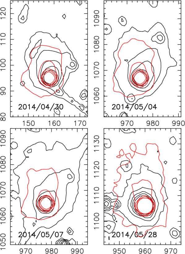
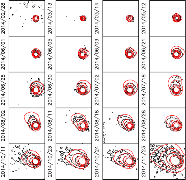
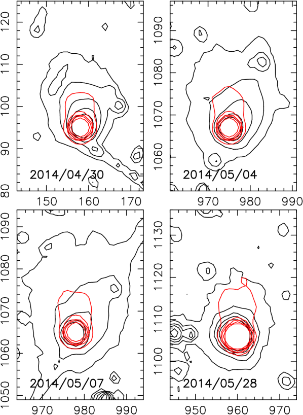
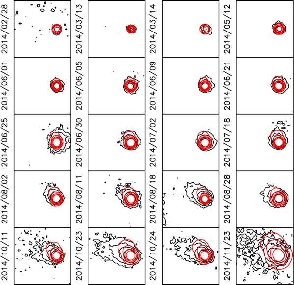
While the modelled images fit the tail shapes for OSIRIS and VLT images until early August 2014 reasonably well, it is clear that they deviate from the measured isophotes at later dates. The total $\chi^{2}$ for this model is 40.1. No improvements are found when Models 2 and 3 are run with different velocity distributions. We therefore tried to modify the input parameters to obtain a better fit to the data. We found that no improvements were possible, except when the power-law index of the size distribution is decreased, i.e. using a steeper size-distribution function. The best results were found for a power index of –3, for which the model results are presented in Figs. 10 and 11 for the NAC and the VLT images, respectively, for Model 1. The corresponding best-fitted dust-loss rate is shown in Fig. 9. For this model, $\chi^{2}$ is 14.4, whcih is much smaller than the value of 40.1 found for the model with power index of –2.

The best-fit power index of –3 for the size-distribution function agrees with that previously derived by Fulle et al. (2010), which was obtained from dust tail modelling of observations that were acquired during several previous orbits. As noted by Fulle et al. (2015a), the different power indices of –2 derived by Rotundi et al. (2015) and of –3 derived from the dust tail models, could be related to contribution of the aggregate particles. The presence of fluffy grains in the coma has been clearly shown by the GIADA instrument since mid-September 2014 (Della Corte et al., 2015; Fulle et al., 2015a). As Rotundi et al. (2015) use earlier measurements, the power index of –2 only refers to the compact particle population. It is possible that those aggregates, which have a steeper size distribution function, are contributing to solve this inconsistency (Fulle et al., 2015a). However, proving it quantitatively is far from easy. First, the computation of the $(1-\mu)$ parameter for aggregates of the order of, or larger than, the wavelength of the incident light is prohibitive in terms of current computational resources. And second, the non-radial pressure force component on the aggregates becomes non-negligible (Kimura et al., 2002), implying a non-Keplerian motion for those particles, and the use of numerical integrators to determine their orbits. In any case, it is interesting to note that the later the observation date, the larger the discrepancy is between the models with size-distribution power indices of –2 and –3 (compare Fig. 8 and Fig. 11).

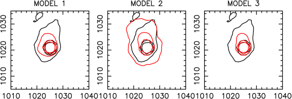
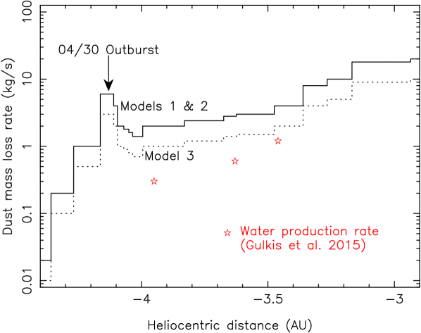
After finding the power index of –3 as the best fit for Model 1, we fit the data with Models 2 and 3, assuming $\alpha$=–3 and leaving the dust-mass loss rate as the only free parameter. The fits to the OSIRIS NAC and VLT data are found in Fig. 12 and Fig. 13 for Model 2, and Fig. 14 and Fig. 15 for Model 3. The models 1, 2, and 3 for the WAC data are shown in Fig. 17, while the corresponding best-fitted dust-loss rate functions are displayed in Fig. 18. Again, a significant deviation of the model isophotes from the observed tail shapes is observed for the VLT data after early August, and particularly for Model 3, which indicates that the particle terminal velocities are better represented by a flat random distribution of velocities rather than a power law of the size, as was found by Rotundi et al. (2015). A proper interpretation of the different particle velocities that were encountered by Rotundi et al. (2015) and Della Corte et al. (2015) should incorporate the hydrodynamical processes in the inner coma, taking into account the different ranges of nucleus to Sun and nucleus to spacecraft distances involved. The computed values of $\chi^{2}$ are 16.1 and 32.8 for models 2 and 3, respectively. As an example, Fig. 16 depicts the resulting scans along the anti-solar direction for one of the latest VLT-observed and modeled images, where the deviations of the data for the different models can be seen.

In Fig. 18, the water production rates at different heliocentric distances that were obtained by Gulkis et al. (2015) from MIRO are also plotted. From these measurements, we obtain a d/g mass ratio varying between 6.5 at 3.95 au pre-perihelion and 3.8 at 3.5 au pre-perihelion, for Models 1 and 2, and between 3.3 at 3.95 au pre-perihelion and 1.6 at 3.5 au pre-perihelion for Model 3, which confirms the d/g=4$\pm$2 that was estimated by Rotundi et al. (2015).

Figure 12: Monte Carlo dust tail code simulations (red contours) compared to the OSIRIS NAC observations (black contours) for the input parameters derived from Rotundi et al. (2015) with a power-law exponent of the size distribution function of –3 and the terminal velocities being given by $v(\mu,t)=1320(1-\mu)^{0.96}u(t)$ m s^-1 (Model 2).

Figure 13: Monte Carlo dust tail code simulations (red contours) compared to the VLT observations (black contours) for the input parameters derived from Rotundi et al. (2015) with a power-law exponent of the size distribution function of –3 and the terminal velocities being given by $v(\mu,t)=1320(1-\mu)^{0.96}u(t)$ m s^-1 (Model 2).

Figure 14: Monte Carlo dust tail code simulations (red contours) compared to the OSIRIS NAC observations (black contours) for the input parameters derived from Rotundi et al. (2015) with a power-law exponent of the size distribution function of –3 and the terminal velocities being given by $v(\mu,t)=45(1-\mu)^{0.42}u(t)$ m s^-1 (Model 3).

Figure 15: Monte Carlo dust tail code simulations (red contours) compared to the VLT observations (black contours) for the input parameters derived from Rotundi et al. (2015), with a power-law exponent of the size distribution function of –3, and the terminal velocities being given by $v(\mu,t)=45(1-\mu)^{0.42}u(t)$ m s^-1 (Model 3).

Figure 16: Scan along the anti-solar direction of the VLT image of 2014/10/24 (solid circles) compared to the different ejection velocity models described in the text: Model 1 (best-fit model) corresponds to the solid-line, Model 2 is represented by the dashed line, and Model 3 by the dotted line. These three models have a power index for the size distribution of –3. The dash-dotted line corresponds to Model 1 but with a power index for the size distribution of –2.

Figure 17: Monte Carlo dust tail code simulations (red contours) compared to the OSIRIS WAC observations (black contours), from left to right, for Models 1, 2, and 3, with a power-law exponent of the size distribution function of –3.

After obtaining this satisfactory fit for Model 1, we explored the sensitivity to the input parameters of the model results. Changing the minimum particle radius from 1 $\mu$m to 10 $\mu$m does not significantly affect the $\chi^{2}$ of the fit, but if the minimum radius is set as high as 50 $\mu$m, $\chi^{2}$ increases by up to 48.2. The presence of dust particles smaller than 5 $\mu$m in size has been demonstrated by Della Corte et al. (2015) from dust accumulation on two of the five micro balances system (MBS) of GIADA since September, 2014. On the other hand, the input dust-mass loss rate can be varied up to the 30% level without altering the model results substantially. Thus, for Model 1, $\chi^{2}$ increases from 14.4 (best fit) to 16.2 by a variation of 30% in the overall dust-mass loss rate. If the dust-loss rate profile is varied up to 50%, then $\chi^{2}$ increases to 19.2, which is too large compared to its equivalent in the best fit model. From this, we estimate a 50% uncertainty as an upper limit to the obtained dust-loss rates.

Figure 18: Best-fit dust-mass loss rate as a function of the heliocentric distance for Models 1 and 2 (solid line), and for Model 3 (dotted line), for power-law size distributions of index –3. Also shown are the water production rates derived from MIRO instrument (Gulkis et al., 2015).

Regarding the level of activity of the comet at the heliocentric distance range explored, we compare the derived dust-loss rates with other published estimates. In most cases, unfortunately, only values of the quantity $Af\rho$ (A’Hearn et al., 1984) have been reported (e.g. Mazzotta Epifani et al., 2009; Kelley et al., 2013b, and references therein), which cannot be easily converted to dust-loss rates. Lamy et al. (2009) gave estimates of a few short-period comets at distances near 3 au, namely 4P/Faye, 17P/Holmes, 44P/Reinmuth, and 71P/Clark. For those comets, the dust-production rate near 3 au ranges from $\sim$1 to 5 kg s^-1, which is less than that derived for 67P ($\sim$15 kg s^-1).

5 Conclusions

A series of Rosetta OSIRIS NAC and WAC images, together with an extensive data set of ground-based VLT images of comet 67P, have been analyzed by our Monte Carlo dust tail model. At the time of the observations, the comet moved from 4.4 au to 2.9 au, inbound. In this heliocentric distance range, the main results can be summarised as follows:

1. The comet was already active at 4.3 au, with a dust-mass loss rate of $\sim$0.5 kg s^-1, increasing up to $\sim$ 15 kg s^-1 at 2.9 au. Based on the model results, these loss rates are affected by a maximum overall uncertainty of $\sim$50%.

2. The dust size distribution is characterised by a power law with a power index of –3 for particles smaller than 1 mm, and –4 for larger grains.

3. The terminal velocity of the particles is best-fitted by a random distribution in the 1 to 5 m s^-1 interval, which is consistent with the in situ measurements of Rotundi et al. (2015).

4. The minimum particle size is constrained at radius $r<$ 10 $\mu$m, while the maximum size is compatible with the innermost coma values derived by Rotundi et al. (2015) ($r$=1 cm).

5. The dust-to-gas mass ratio, based on the results of our best-fit model and combined with water production rates that were inferred from the MIRO experiment, varies between 3.8 and 6.5, which is consistent with the value of 4$\pm$2 derived by Rotundi et al. (2015).

Appendix A Log of VLT/FORS2 observations

Table 2: Observational circumstances for the VLT/FORS2 observations

Date	r	Earth-comet	Phase angle	Position angle	Resolution
dd.dd mm yyyy (UT)	(au)	distance (au)	(deg)	(deg)	(km px-1)
28.39 2 2014	4.386	4.909	10.40	259.27	890.1
13.37 3 2014	4.330	4.680	11.86	264.37	848.6
14.37 3 2014	4.326	4.661	11.96	259.27	845.2
15.34 3 2014	4.321	4.643	12.06	259.27	841.9
10.41 4 2014	4.204	4.133	13.77	259.65	749.5
4.37 5 2014	4.092	3.655	13.50	261.28	662.7
7.26 5 2014	4.078	3.599	13.32	261.61	652.7
12.40 5 2014	4.053	3.502	12.91	262.32	635.0
1.32 6 2014	3.954	3.159	10.22	266.94	572.8
5.12 6 2014	3.934	3.101	9.51	268.37	562.3
6.20 6 2014	3.929	3.085	9.30	268.82	559.5
9.32 6 2014	3.913	3.041	8.65	270.29	551.4
10.22 6 2014	3.908	3.029	8.46	270.76	549.2
19.37 6 2014	3.861	2.915	6.34	277.39	528.5
20.28 6 2014	3.856	2.904	6.11	278.33	526.6
21.17 6 2014	3.851	2.895	5.89	279.30	524.9
25.05 6 2014	3.830	2.855	4.92	284.60	517.6
30.20 6 2014	3.804	2.808	3.64	296.05	509.2
1.13 7 2014	3.799	2.801	3.43	298.98	507.9
2.09 7 2014	3.793	2.793	3.21	302.45	506.5
7.05 7 2014	3.767	2.759	2.35	329.65	500.2
15.07 7 2014	3.723	2.719	2.77	29.61	492.9
16.08 7 2014	3.718	2.715	2.98	34.69	492.3
18.10 7 2014	3.707	2.708	3.44	42.98	491.1
21.03 7 2014	3.690	2.701	4.20	51.65	489.8
22.01 7 2014	3.685	2.699	4.47	53.92	489.4
24.24 7 2014	3.673	2.696	5.09	58.24	488.9
26.23 7 2014	3.662	2.694	5.66	61.35	488.6
2.21 8 2014	3.622	2.697	7.66	68.88	489.1
4.16 8 2014	3.611	2.701	8.21	70.40	489.7
11.99 8 2014	3.567	2.723	10.32	75.05	493.7
15.99 8 2014	3.544	2.739	11.33	76.82	496.7
16.98 8 2014	3.538	2.744	11.57	77.22	497.5
18.00 8 2014	3.532	2.749	11.81	77.61	498.4
28.98 8 2014	3.467	2.814	14.16	80.99	510.2
23.16 9 2014	3.315	3.016	17.42	85.11	546.9
11.05 10 2014	3.203	3.172	18.01	86.22	575.2
12.05 10 2014	3.197	3.181	18.00	86.25	576.7
18.05 10 2014	3.158	3.231	17.90	86.40	585.8
19.07 10 2014	3.152	3.239	17.87	86.41	587.3
23.02 10 2014	3.126	3.270	17.71	86.45	593.0
24.02 10 2014	3.120	3.278	17.66	86.46	594.4
25.07 10 2014	3.113	3.286	17.61	86.46	595.8
26.01 10 2014	3.107	3.293	17.56	86.46	597.1
15.05 11 2014	2.974	3.423	15.88	86.27	620.7
17.05 11 2014	2.961	3.434	15.65	86.24	622.6
18.02 11 2014	2.954	3.438	15.54	86.22	623.4
19.02 11 2014	2.947	3.443	15.42	86.21	624.3
20.06 11 2014	2.940	3.448	15.30	86.19	625.2
21.02 11 2014	2.934	3.453	15.18	86.18	626.0
23.02 11 2014	2.920	3.461	14.93	86.15	627.6
24.05 11 2014	2.913	3.466	14.79	86.14	628.4

References

- Agarwal et al. (2010) Agarwal, J., Müller, M., Reach, W.T. et al. 2010, Icarus, 207, 992
- A’Hearn et al. (1984) A’Hearn, M., Millis, R.L., Schleicher, D.G., et al. 1984, ApJ, 89, 579
- Bramich (2008) Bramich, D.M. 2008, MNRAS, 386, L77
- Colangeli et al. (2009) Colangeli, L., López-Moreno, J. J., Palumbo, P., et al. 2009, The GIADA instrument, in Rosetta ESA’s mission to the Origin of the Solar System, ed. R. Schulz, C. Alexander, H. Böhnhardt, & K. H. Glassmeier (Springer) 243
- Crifo et al. (2004) Crifo, J. F., Fulle, M., Kömle, N. I., & Szego, K. 2004, Nucleus-coma structural relationships: lessons from physical models, in Comets II, ed. M. C. Festou, H. U. Keller, & H. A. Weaver (Tucson: University of Arizona Press) 471
- Della Corte et al. (2014) Della Corte, V., Rotundi, A., Accolla, M., et al. 2014, Journal Astron. Instr., 1350011
- Della Corte et al. (2015) Della Corte, V., Rotundi, A., Fulle, M. et al. 2015, A&A, 583, A13
- Finson & Probstein (1968) Finson, M. & Probstein, M. 1968, ApJ, 154,327
- Fornasier et al. (2015) Fornasier, S., Hasselmann, P.H., Barucci, M.A. et al. 2015, A&A, 583, A30
- Fulle (1989) Fulle, M. 1989, A&A, 217, 283
- Fulle et al. (2010) Fulle. M., Colangeli, L., Agarwal, J., et al. 2010, A&A, 522, A63
- Fulle et al. (2015a) Fulle, M., Della Corte, V., Rotundi, A., et al. 2015a, ApJ, 802, L12.
- Fulle et al. (2015b) Fulle, M., et al. 2015b, in preparation
- Gulkis et al. (2015) Gulkis, S., Allen, M., von Allmen, P., et al. 2015, Science, 347, aaa0709
- Keller et al. (2007) Keller, H. U., Barbieri, C., Lamy, P., et al. 2007, Space Sci. Rev., 128, 433
- Kelley et al. (2013a) Kelley, M.S., Lindler, D.J., Bodewits, D., et al. 2013a, Icarus, 222, 634
- Kelley et al. (2013b) Kelley, M.S., Fernández, Y.R., Licandro, J., et al. 2013b, Icarus, 225, 475
- Kimura et al. (2002) Kimura, H., Okamoto, H., and Mukai, T. 2002, Icarus, 157, 349
- Lamy et al. (2006) Lamy, P.L., Toth, I., Weaver, H.A., et al. 2006, A&A, 458, 669
- Lamy et al. (2009) Lamy, P.L., Toth, I., Weaver, H.A., et al. 2009, A&A, 508, 1045
- Lara et al. (2015) Lara, L. M., Gutiérrez, P., Lowry, S., et al. 2015, A&A, 583, A9
- Mazzotta Epifani et al. (2009) Mazzotta Epifani, E., Palumbo, P., & Colangeli, L. 2009, A&A, 508, 1031
- Meech & Jewitt (1987) Meech, K.J., & Jewitt, D.C. 1987, A&A, 187, 585
- Montalto et al. (2008) Montalto, M., Riffeser, A., Hopp, U., et al. 2008, A&A 479, L45
- Mottola et al. (2014) Mottola, S., Lowry, S., Snodgrass, C. et al. 2014, A&A, 569, L2
- Mottola et al. (2015) Mottola, S., Arnold, G., Grothues, H.-G., et al. 2015, Science, 349, aab0232
- Moreno et al. (2008) Moreno, F., Ortiz, J.L., Santos-Sanz, P. et al. 2008, ApJ, 677, L63
- Moreno et al. (2012) Moreno, F., Pozuelos, F., Aceituno, F., et al. 2012, ApJ, 752, 136
- Preusker et al. (2015) Preusker, F., Scholten, F., Matz K. D., et al. 2015, A&A, 583, A33
- Rotundi et al. (2015) Rotundi, A., Sierks, H., Della Corte, V., et al. 2015, Science, 347, aaa3905
- Schulz et al. (2015) Schulz, R., Hilchenbach, M., Langevin, Y. et al. 2015, Nature, 518, 216
- Sierks et al. (2015) Sierks, K., Barbieri, C., Lamy, P. L., et al. 2015, Science, 347, aaa1044
- Snodgrass et al. (2013) Snodgrass, C., Tubiana, C., Bramich, D.M. et al. 2013, A&A, 557, A33
- Snodgrass et al. (2015) Snodgrass, C., Jehin, E., Manfroid, J. et al. 2015, submitted
- Soja et al. (2015) Soja, R.H., Sommer, M., Herzog, J., et al. 2015, A&A, 583, A18
- Tubiana et al. (2015a) Tubiana C., Snodgrass, C., Bertini, I., et al. 2015a, A&A, 573, A62
- Tubiana et al. (2015b) Tubiana C., Güttler, C., Kovacs, G., et al. 2015b, A&A, 583, A46
- Whipple (1950) Whipple, F. 1950, ApJ, 111, 375