Magnetic order and spin excitations in the Kitaev–Heisenberg model on the honeycomb lattice

Abstract

We consider the quasi-two-dimensional pseudo-spin-1/2 Kitaev - Heisenberg model proposed for A₂IrO₃ (A=Li, Na) compounds. The spin-wave excitation spectrum, the sublattice magnetization, and the transition temperatures are calculated in the random phase approximation (RPA) for four different ordered phases, observed in the parameter space of the model: antiferomagnetic, stripe, ferromagnetic, and zigzag phases. The Néel temperature and temperature dependence of the sublattice magnetization are compared with the experimental data on Na₂IrO₃.

I Introduction

Recent studies of transition-metal oxides have revealed an important role of the orbital degrees of freedom which bring about highly anisotropic spin interactions and complicated magnetic properties of these materials (for a review see  Khaliullin05 ; Nussinov15 ). Particularly, fascinating phase diagrams have been observed for the $4d$ and $5d$ transition-metal oxides. In comparison with $3d$ compounds, they have weaker Coulomb correlations due to a delocalized character of $4d$ and $5d$ states, but a much stronger relativistic spin-orbit coupling (SOC). The latter entangles the spin and orbital degrees of freedom, and a new type of quantum state bands emerges determined by the effective total angular moment $J_{eff}$. For the iridium-based compounds with 5d electrons on $t_{2g}$ orbitals in the magnetic ion Ir⁴⁺, a strong SOC splits the broad $t_{2g}$ band into $J_{eff}=3/2$ and $J_{eff}=1/2$ subbands. Then even a weak Coulomb correlation brings about a Mott insulating state in the half-filled $J_{eff}=1/2$ band Kim08 . Based on the consideration of crystal-field splitting and SOC for layered iridium compounds, an effective Heisenberg model for the pseudospins $S=1/2$ with the compass-model anisotropy was proposed in Ref. Jackeli09 :

$$H=J\sum_{\langle ij\rangle}{\bf S}_{i}\cdot{\bf S}_{j}+K\sum_{\langle ij\rangle_{\gamma}}S_{i}^{\gamma}S_{j}^{\gamma},$$ (1)

where $J$ is the isotropic Heisenberg interaction for nearest neighbors (n.n.) $\langle ij\rangle$ and $K$ is the n.n. $\langle ij\rangle_{\gamma}$ bond-dependent Kitaev interaction Kitaev06 . The superexchange interaction on the square lattices in A₂IrO₃ compounds (A = Na, Ba) with corner-sharing oxygen octahedra is predominantly of the isotropic Heisenberg type $J$, while for the honeycomb lattices in A₂IrO₃ compounds (A = Li, Na) with edge-sharing oxygen octahedra the anisotropic Kitaev interaction $K$ dominates. The exact solution of the Kitaev model Kitaev06 reveals a highly frustrated quantum spin-liquid phase with peculiar dynamics  Knolle14 ; Knolle14a ; Knolle15 . The inclusion of a finite isotropic Heisenberg interaction $J$ lifts the degeneracy of the ground state, and a rich phase diagram with competing long-range orders, such as the ferromagnetic (FM), antiferromagnetic (AF), stripe and zigzag phases, emerges Chaloupka10 ; Chaloupka13 .

The parameters of the Kitaev-Heisenberg (KH) model (1) for Na₂IrO₃ were calculated using the density functional theory Kim12 ; Kim13 ; Foyevtsova13 ; Yamaji14 , ab initio quantum chemistry calculations Katukuri14 ; Nishimoto14 , and microscopic superexchange calculations Sizyuk14 . As a general conclusion it was found that for Na₂IrO₃ the n.n. Kitaev interaction is FM and much stronger than the AF Heisenberg interaction, e.g., $K\simeq-17$ meV, $\,J\simeq 3$ meV Katukuri14 . For Li₂IrO₃ a strong dependence of the coupling constant on the parameters of Ir-O bonds was found so that the n.n. Heisenberg interaction $J$ has opposite signs for the two inequivalent Ir - Ir links: $J\approx-19$ meV and $J\approx 1$ meV for another link Nishimoto14 . It was also found that the next n.n. Heisenberg and Kitaev interactions are comparable to the n.n. contributions, and they should be taken into account to describe the experimentally observed zigzag phase. In the absence of next n.n. interactions in the KH model (1) the zigzag phase can be obtained only for AF Kitaev and FM Heisenberg interactions, e.g., $K\simeq 21$ meV, $\,J\simeq-4$ meV, as was proposed in Refs. Chaloupka10 ; Chaloupka13 . Depending on the values of the second ($J_{2}$) and third ($J_{3}$) neighbor Heisenberg interactions, a complicated phase diagram emerges with an incommensurate magnetic order in a large part of the diagram Sizyuk14 . An important role of the further-distant-neighbor interactions and of the bond-depending off-diagonal exchange interaction was also stressed in other publications (see Refs. Kimchi11 ; Singh12 ; Rau14 ; Lou15 ).

The ground-state properties and excitation spectrum of the KH model have been studied by various methods, such as the Lanczos exact diagonalization for finite clusters Chaloupka10 ; Chaloupka13 ; Rau14 , pseudofermion renormalization group Reuther11 , classical Monte Carlo simulation Sizyuk14 ; Price12 ; Price13 , tensor variational approachIregui14 , and the entanglement renormalization ansatz Lou15 . The spectrum of spin waves in the KH model was calculated within linear spin-wave theory (LSWT) in the zigzag phase in Ref. Chaloupka13 . In Refs. You12 ; Hyart12 ; Okamoto13 doping effects on the phase diagram and emerging superconductivity in the extended KH model were studied within a generalized $t$-$J$ model.

Most of experimental studies are devoted to Na₂IrO₃. Measurements of electrical resistivity, magnetization, magnetic susceptibility, and heat capacity of Na₂IrO₃ have shown a phase transition to the long-range AF order below $T_{N}=15$ K Singh10 . In Ref. Liu11 , using resonant x-ray scattering, the AF phase transition was found at $T_{N}=13.3$ K, and the zigzag magnetic structure was proposed. A direct evidence of the zigzag magnetic phase was obtained by neutron and x-ray diffraction investigations of Na₂IrO₃ single crystals below $T_{N}=18$ K Ye12 . In Ref. Choi12 the spectrum of spin excitations in Na₂IrO₃ was measured by inelastic neutron scattering which confirmed the zigzag magnetic order. The spin-wave spectrum was observed below $5$ mev and was described within LSWT for the Heisenberg model with the exchange interaction up to the third neighbors, while the contribution from the Kitaev interaction was considered to be small. The long-range magnetic order below $T_{N}=15.3$ K in this study was detected by the muon-spin rotation method. Magnetic excitations in Na₂IrO₃ were also investigated in Ref. Gretarsson13 using resonant inelastic x-ray scattering. Excitations with much higher energy of about $35$ meV were observed at the $\Gamma$ point in the Brillouin zone with the dispersion consistent with the calculation in Ref. Chaloupka13 . In Ref. Comin12 optical and angle-resolved photoemission spectroscopy on Na₂IrO₃ revealed an insulating gap of 340 meV which can be explained by suggesting a large Coulomb repulsion $U=3$ eV in the Mott insulating state. In Ref. Singh12 roughly the same temperatures of the magnetic phase transition, $T_{N}\approx 15$ K, in A₂IrO₃ for A= Na and Li were reported using magnetic and heat capacity measurements .

In the present paper we perform self-consistent calculations of the sublattice magnetization and the spin-wave excitation spectrum for the KH model (1) on the honeycomb lattice. We consider the full parameter space of the model, where four ordered phases are known to exist. To take into account the finite-temperature renormalization of the spectrum and to calculate the transition temperature $T_{c}$, we employ the equation of motion method for Green functions (GFs) Zubarev60 for spin $S=1/2$ using the random phase approximation (RPA) Tyablikov75 , as we have done for the compass-Heisenberg model on the square lattice in Ref. Vladimirov14 .

In Sec. II we formulate the KH model and derive equations for the matrix GF. The magnetization and phase transition temperatures for all four phases are considered in Sec. III. The results of spin-wave spectrum calculations and for the phase diagram are presented in Sec. IV. They are compared with experiments on A₂IrO₃ and other theoretical studies of the KH model. In Sec. V the conclusion is given, and in the Appendix details of calculations are presented.

II Spin-excitation spectrum

II.1 Kitaev-Heisenberg model

We consider the KH model on the honeycomb lattice with the n.n. distance $a_{0}$. The lattice is bipartite with two sublattices $A$ and $B$.

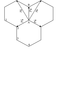
Figure 1: Honeycomb lattice, where $\overrightarrow{\delta_{1}},\,\overrightarrow{\delta_{2}},\,\overrightarrow{\delta_{3}}$ are the nearest-neighbour vectors (2), ${\bf a}_{1}$ and ${\bf a}_{2}$ are the lattice vectors. The four sublattices in the zigzag and stripe phases are denoted by the numbers $1,2,3,4$.

Each lattice site on $A$ is connected to three n. n. sites belonging to $B$ by vectors $\overrightarrow{\delta_{j}}$, sites on $B$ sublattice are connected to $A$ by vectors $-\overrightarrow{\delta_{j}}$ (see Fig. 1):

$$\overrightarrow{\delta_{1}}=\frac{a_{0}}{2}(\sqrt{3},-1),\;\overrightarrow{\delta_{2}}=-\frac{a_{0}}{2}(\sqrt{3},1),\;\overrightarrow{\delta_{3}}=a_{0}(0,1).$$ (2)

The lattice vectors are ${\bf a}_{1}=\overrightarrow{\delta_{3}}-\overrightarrow{\delta_{2}}=({a_{0}}/{2})(\sqrt{3},3)$ and ${\bf a}_{2}=\overrightarrow{\delta_{3}}-\overrightarrow{\delta_{1}}=({a_{0}}/{2})(-\sqrt{3},3)$, the lattice constant is $a=|{\bf a}_{1}|=|{\bf a}_{2}|=\sqrt{3}a_{0}$. The reciprocal lattice is defined by the vectors ${\bf k}_{1}=({2\pi}/{3a_{0}})(\sqrt{3},1)$ and ${\bf k}_{2}=({2\pi}/{3a_{0}})(-\sqrt{3},1)$.

The KH model (1) is convenient to write in a short notation as:

$$H=\sum_{i,m,\nu}J^{\nu}_{m}S^{\nu}_{i}S^{\nu}_{i+m}.$$ (3)

Here, $i$ goes over all sites of the $A$ sublattice, and $i+m$ denotes n.n. sites of $i$, which belong to the $B$ sublattice, ${\bf r}_{i+m}={\bf r}_{i}+\overrightarrow{\delta_{m}}$. The exchange interaction $J^{\nu}_{m}$ depends on the spin component index $\nu=x,y,z$ and the bond number $m=1,2,3$. In the particular case of the KH model, the exchange interaction reads as $J^{\nu}_{1}=(J+K_{x},J,J),J^{\nu}_{2}=(J,J+K_{y},J),J^{\nu}_{3}=(J,J,J+K_{z})$ where we can also consider an anisotropic Kitaev interaction, $K_{x}\neq K_{y}\neq K_{z}$.

In the general case we consider several sublattices for the model (3) with the sublattice vectors ${\bf b}_{j}$, where $j$ is the sublattice index, ${\bf b}_{1}\equiv 0$, ${\bf b}_{2}$ connects the first sublattice to the second one, etc. Any vector connecting sites on the same sublattice is a combination of the lattice vectors ${\bf a}_{1}$, ${\bf a}_{2}$. All ${\bf a}$ and ${\bf b}$ vectors are combinations of $\overrightarrow{\delta_{i}}$. To study the zigzag phase, we have to consider the four sublattice representation as in Refs. Choi12 ; Chaloupka10 ; Chaloupka13 .

Using the spin operators $S^{\pm}_{i}=S^{x}_{i}\pm iS^{y}_{i},\,S^{z}_{i}$, the Hamiltonian (3) can be written as:

$$H=\sum_{i,j,k,l} J^{z}_{i,j,k,l}S^{z}_{i,j}S^{z}_{k,l}+\frac{1}{2}J^{+}_{i,j,k,l}(S^{+}_{i,j}S^{-}_{k,l}+S^{-}_{i,j}S^{+}_{k,l})$$ (4)

$$+\frac{1}{2}J^{-}_{i,j,k,l}(S^{+}_{i,j}S^{+}_{k,l}+S^{-}_{i,j}S^{-}_{k,l}),$$

with $J^{\pm}_{i,j,k,l}=(1/2)(J^{x}_{i,j,k,l}\pm J^{y}_{i,j,k,l})$. Here $i$,$k$ are lattice indexes, and $j$,$l$ are sublattice indexes. The honeycomb lattice has two nonequivalent sites $A$ and $B$ per unit cell. If we have more then two sublattices, we can define them in such a way, that lattice sites with odd (even) sublattice indexes belong to the sublattice $A(B)$. Then the interaction parameters $J^{\nu}$ for $\nu\in\{z,+,-\}$ have the form: $J^{\nu}_{i,j,k,l}=\sum_{m}J^{\nu}_{m}\delta[{\bf a}_{k}+{\bf b}_{l}-{\bf a}_{i}-{\bf b}_{j}+(-1)^{j}\overrightarrow{\delta_{m}}]$, where $\sum_{m}\delta[{\bf a}_{k}+{\bf b}_{l}-{\bf a}_{i}-{\bf b}_{j}+(-1)^{j}\overrightarrow{\delta_{m}}]$ is equal to unity if the $(k,l)$ site is n.n. of the $(i,j)$ site. The components $J^{\nu}_{m}$ are given by $J^{z}_{1}=J^{z}_{2}=J$, $J^{z}_{3}=J+K_{z}$, $J^{+}_{1}=J+K_{x}/2$, $J^{+}_{2}=J+K_{y}/2$, $J^{+}_{3}=J$, $J^{-}_{1}=K_{x}/2$, $J^{-}_{2}=-K_{y}/2$, $J^{-}_{3}=0$.

II.2 Green function equations

To calculate the spin-wave spectrum of transverse spin excitations, we introduce the matrix retarded two-time commutator GF Zubarev60 :

$$\hat{G}(t-t^{\prime})=-i\theta(t-t^{\prime})\langle[\hat{S}(t)\;,\;\hat{S}^{{\dagger}}(t^{\prime})]\rangle$$

$$=\int_{-\infty}^{+\infty}\,\frac{d\omega}{2\pi}\,e^{-i\omega(t-t^{\prime})}\hat{G}(\omega),$$ (5)

where

$$\hat{G}(\omega)=\left(\begin{array}[]{cccc}\langle\!\langle S^{+}_{i,j}|S^{-}_{i^{\prime},j^{\prime}}\rangle\!\rangle_{\omega}\;\langle\!\langle S^{-}_{i,j}|S^{-}_{i^{\prime},j^{\prime}}\rangle\!\rangle_{\omega}\\ \langle\!\langle S^{+}_{i,j}|S^{+}_{i^{\prime},j^{\prime}}\rangle\!\rangle_{\omega}\;\langle\!\langle S^{-}_{i,j}|S^{+}_{i^{\prime},j^{\prime}}\rangle\!\rangle_{\omega}\\ \end{array}\right).$$ (8)

Using the commutation relations for spin operators, $\,[{S_{i}^{+}},{S_{j}^{-}}]=2{S_{i}^{z}}\,\delta_{i,j},\quad[{S_{i}^{\pm}},{S_{j}^{z}}]=\mp{S_{i}^{\pm}}\,\delta_{i,j},\,$ we obtain equations of motion for the GFs

$$\omega\langle\!\langle S_{i,j}^{+}|S_{i^{\prime},j^{\prime}}^{-}\rangle\!\rangle_{\omega}=2\langle S^{z}_{i,j}\rangle\,\delta_{i,i^{\prime}}\delta_{j,j^{\prime}}$$

$$-\sum_{k,l}\,J^{z}_{i,j,k,l}\langle\!\langle\,S^{+}_{i,j}S^{z}_{k,l}|S_{i^{\prime},j^{\prime}}^{-}\rangle\!\rangle_{\omega}$$

$$+\sum_{k,l}J^{+}_{i,j,k,l}\langle\!\langle\,S^{z}_{i,j}S^{+}_{k,l}|S_{i^{\prime},j^{\prime}}^{-}\rangle\!\rangle_{\omega}$$

$$+\sum_{k,l}\,J^{-}_{i,j,k,l}\langle\!\langle\,S^{z}_{i,j}S^{-}_{k,l}|S_{i^{\prime},j^{\prime}}^{-}\rangle\!\rangle_{\omega},$$ (9)

$$\omega\langle\!\langle S_{i,j}^{-}|S_{i^{\prime},j^{\prime}}^{+}\rangle\!\rangle_{\omega}=-2\langle S^{z}_{i,j}\rangle\,\delta_{i,i^{\prime}}\delta_{j,j^{\prime}}$$

$$+\sum_{k,l}\,J^{z}_{i,j,k,l}\langle\!\langle\,S^{-}_{i,j}S^{z}_{k,l}|S_{i^{\prime},j^{\prime}}^{+}\rangle\!\rangle_{\omega}$$

$$-\sum_{k,l}J^{+}_{i,j,k,l}\langle\!\langle\,S^{z}_{i,j}S^{-}_{k,l}|S_{i^{\prime},j^{\prime}}^{+}\rangle\!\rangle_{\omega}$$

$$-\sum_{k,l}\,J^{-}_{i,j,k,l}\langle\!\langle\,S^{z}_{i,j}S^{+}_{k,l}|S_{i^{\prime},j^{\prime}}^{+}\rangle\!\rangle_{\omega}.$$ (10)

In the RPA Tyablikov75 for all GFs we use the following approximation:

$$\langle\!\langle S_{i,j}^{z}S_{k,l}^{\alpha}|S_{i^{\prime},j^{\prime}}^{\beta}\rangle\!\rangle_{\omega} =s(j)\sigma\,\langle\!\langle S_{k,l}^{\alpha}|S_{i^{\prime},j^{\prime}}^{\beta}\rangle\!\rangle_{\omega},$$ (11)

where $\sigma$ is the absolute value of the order parameter while $s(j)=\pm 1$ is the sublattice-dependent sign of the order parameter. By choosing $s(j)$ we can describe different phases in our model.

Using the momentum representation with respect to the lattice index $i$,

$$S_{i,j}^{\pm}=\sqrt{\frac{1}{N}}\sum_{\bf q}\,S^{\pm}_{{\bf q},j}\,{\rm e}^{{\pm}i{\bf q}({\bf a}_{i}+{\bf b}_{j})},$$

$$J^{\nu}_{{\bf q},j,l}=\frac{1}{N}\sum_{i,k}J^{\nu}_{i,j,k,l}{\rm e}^{i{\bf q}({\bf a}_{k}+{\bf b}_{l}-{\bf a}_{i}-{\bf b}_{j})},$$ (12)

where $N$ is number of sites per sublattice, and introducing the nonation:

$$\gamma^{z}_{j}=\sum_{l}\,s(l)J^{z}_{0,j,l},\;\;\;\;\gamma^{\pm}_{{\bf q},j,l}=s(j)J^{\pm}_{{\bf q},j,l},$$ (13)

Eqs. (9) and (10) for the GFs in the RPA (11) can be written as

$$\omega\langle\!\langle S_{{\bf q},j}^{+}|S_{{\bf q},j}^{-}\rangle\!\rangle_{\omega}=2\sigma s(j)-\sigma\gamma^{z}_{j}\langle\!\langle\,S^{+}_{{\bf q},j}|S_{{\bf q},j}^{-}\rangle\!\rangle_{\omega}$$ (14)

$$+\sigma\sum_{l}\gamma^{+}_{{\bf q},j,l}\langle\!\langle\,S^{+}_{{\bf q},l}|S_{{\bf q},j}^{-}\rangle\!\rangle_{\omega}+\sigma\sum_{l}\gamma^{-}_{{\bf q},j,l}\langle\!\langle\,S^{-}_{{-\bf q},l}|S_{{\bf q},j}^{-}\rangle\!\rangle_{\omega},$$

$$\omega\langle\!\langle S_{{\bf q},j}^{-}|S_{{\bf q},j}^{+}\rangle\!\rangle_{\omega}=-2\sigma s(j)+\sigma\gamma^{z}_{j}\langle\!\langle\,S^{-}_{{\bf q},j}|S_{{\bf q},j}^{+}\rangle\!\rangle_{\omega}$$ (15)

$$-\sigma\sum_{l}\gamma^{+}_{{\bf q},j,l}\langle\!\langle\,S^{-}_{{\bf q},l}|S_{{\bf q},j}^{+}\rangle\!\rangle_{\omega}-\sigma\sum_{l}\gamma^{-}_{{\bf q},j,l}\langle\!\langle\,S^{+}_{{\bf q},l}|S_{{-\bf q},j}^{+}\rangle\!\rangle_{\omega}.$$

The system of $\,2n\,$ equations for $n$ sublattices can be written in the matrix form:

$$\omega\langle\!\langle\,\mathbb{S}|\mathbb{S}^{\dagger}\rangle\!\rangle_{{\bf q},\omega}=\hat{\sigma}+\sigma\hat{V}(\bf q)\langle\!\langle\,\mathbb{S}|\mathbb{S}^{\dagger}\rangle\!\rangle_{{\bf q},\omega},$$ (16)

where $\mathbb{S}=[S^{+}_{1},S^{-}_{1},S^{+}_{2},S^{-}_{2}...]$, $\hat{\sigma}=[2\sigma s(1),-2\sigma s(1),2\sigma s(2),-2\sigma s(2)...]$, and $\hat{V}$ is the matrix of the $\gamma$ coefficients (13). This system of equations has the solution

$$\langle\!\langle\,\mathbb{S}|\mathbb{S}^{\dagger}\rangle\!\rangle_{{\bf q},\omega}=[\,\omega\hat{I}-\sigma\hat{V}(\bf q)]^{-1}\hat{\sigma},$$ (17)

where $\hat{I}$ is the unity matrix. The spectrum of spin excitations is given by the eigenvalues of the matrix $\sigma\hat{V}$.

III Magnetic order

To calculate the sublattice magnetization $\sigma=\langle S_{i}^{z}\rangle$ in RPA, we use the kinematic relation $\,S_{i}^{z}=(1/2)-S_{i}^{-}S_{i}^{+}\,$ for spin $S=1/2$ which results in the self-consistent equation

$$\sigma=\langle S_{i}^{z}\rangle=\frac{1}{2}-\frac{1}{N}\sum_{\bf q}\,\langle S^{-}_{\bf q}S^{+}_{\bf q}\rangle.$$ (18)

The correlation function in Eq. (18) is calculated from the GF (17) using the spectral representation,

$$\langle S^{-}_{\bf q}S^{+}_{\bf q}\rangle=2\sigma\,\sum_{i}I_{i}({\bf q})\,N[\omega_{i}({\bf q})]\,,$$ (19)

where $N(\omega)=[\exp(\omega/T)-1]^{-1}$, $\omega_{i}({\bf q})=\sigma\varepsilon_{i}({\bf q})$, $\varepsilon_{i}({\bf q})$ are eigenvalues of $\hat{V}(\bf q)$, and

$$I_{i}({\bf q})=\frac{a^{11}_{\bf q}[\varepsilon_{i}({\bf q})]}{\prod_{j\neq i}[\varepsilon_{i}({\bf q})-\varepsilon_{j}({\bf q})]}.$$ (20)

Here $a^{11}_{\bf q}[\varepsilon_{i}({\bf q})]$ is the $(1,1)$ first minor of the $[\varepsilon\hat{I}-\hat{V}(\bf q)]$ matrix.

By taking the limit $\sigma\rightarrow 0$ we can also obtain an equation for the Néel temperature:

$$\frac{1}{T_{N}}=\frac{4}{N}\sum_{\bf q}\,\sum_{i}\frac{I_{i}({\bf q})}{\varepsilon_{i}({\bf q})}.$$ (21)

The sum over ${\bf q}$ in this equation will diverge in the two-dimensional (2D) case if the spin excitation spectrum has no gaps, i.e., $\varepsilon_{i}({\bf Q})=0$ at some momentum ${\bf Q}$. In this case, in order to obtain a finite transition temperature, we either should consider the 3D case introducing an inter-plane coupling $J_{\bot}$ (either FM or AF) or add a small anisotropy to the Kitaev interaction, e.g., $K_{z}>K_{y}=K_{x}$. This opens a gap at this wave vector, as discussed in the next section.

IV Results and discussion

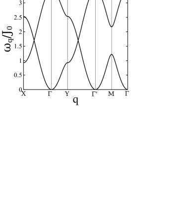
Figure 2: Spin-wave spectrum for the FM phase at $\phi=200^{\circ}$, where $J=J_{0}\,\cos\phi$, $K=2\,J_{0}\,\sin\phi$ .

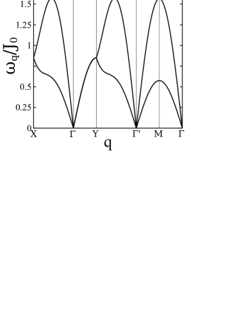
Figure 3: Spin-wave spectrum for the AF phase at $\phi=50^{\circ}$.

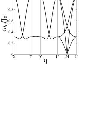
Figure 4: Spin-wave spectrum for the zigzag phase at $\phi=110.85^{\circ}$.

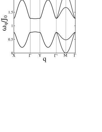
Figure 5: Spin-wave spectrum for the atripe phase at $\phi=300^{\circ}$.

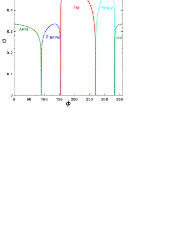
Figure 6: (Color online) Magnetization for different phases at zero temperature versus phase angle $\phi$.

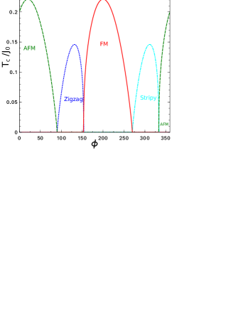
Figure 7: (Color online) Transition temperature for different phases versus phase angle $\phi$ at $J_{\bot}=-0.0018\,J_{0}$.

Figure 8: Neél temperature $T_{N}$ as a function of the interplane coupling $J_{\bot}=-\eta J_{0}$ (solid line) and anisotropy $K_{z}=(1+\eta)K$, $K_{x}=K_{y}=K$ (dashed line), with $J=-4$ meV, $K=21$ meV, compared with the experimental Neél temperature of Na₂IrO₃ (thin line) from Choi12 .

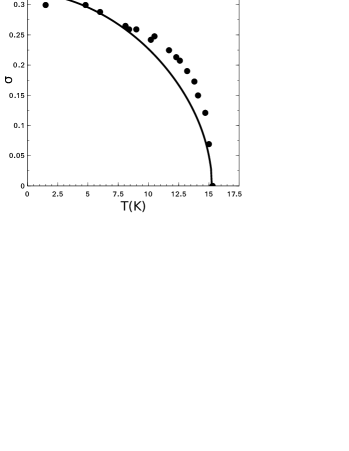
Figure 9: Sublattice magnetization $\sigma$ as a function of temperature in the zigzag phase for $J=-4$ meV, $K=21$ meV, $J_{\bot}=-0.02$ meV (solid line), compared with experimental data on Na₂IrO₃ from Choi12 in arbitrary units (circles).

In this section we calculate the spin-wave spectrum $\omega_{i}({\bf q})$ for the AF, FM, zigzag, and stripe phases by solving Eq. (17) and determine self-consistently the sublattice magnetization $\sigma=\langle S_{i}^{z}\rangle$ in these phases using Eq. (18). In the equations for the spin-wave spectra we introduce the short notations: $c_{x}=\cos(\frac{\sqrt{3}}{2}a_{0}q_{x})$, $s_{x}=\sin(\frac{\sqrt{3}}{2}a_{0}q_{x})$, $c_{y}=\cos(\frac{3}{2}a_{0}q_{y})$, and $s_{y}=\sin(\frac{3}{2}a_{0}q_{y})$. In the AF phase we get:

$$\varepsilon^{2}_{\pm}({\bf q})=A^{2}+|B_{\bf q}|^{2}-|C_{\bf q}|^{2}\pm 2\sqrt{A^{2}|B_{\bf q}|^{2}-[{\rm Im}(B_{\bf q}C^{*}_{\bf q})]^{2}},$$ (22)

In the FM phase we have:

$$\varepsilon^{2}_{\pm}({\bf q})=A^{2}-|B_{\bf q}|^{2}+|C_{\bf q}|^{2}\pm 2\sqrt{A^{2}|C_{\bf q}|^{2}-[{\rm Im}(B_{\bf q}C^{*}_{\bf q})]^{2}}.$$ (23)

Here

$$A = 3J+K_{z},$$

$$|B_{\bf q}|^{2} = K_{+}^{2}-K_{x}K_{y}c_{x}^{2},$$

$$|C_{\bf q}|^{2} = [(2J+K_{+})c_{x}+Jc_{y}]^{2}$$

$$+ (Js_{y}+K_{-}s_{x})^{2},$$

$${\rm Im}(B_{\bf q}C^{*}_{\bf q}) = K_{+}s_{x}[(2J+K_{+})c_{x}+Jc_{y}]$$ (24)

$$- K_{-}c_{x}(K_{-}s_{x}-Js_{y}),$$

where $\,K_{\pm}=(K_{x}\pm K_{y})/2\,$. For the zigzag phase we obtain Eq. (38) which for the isotropic intaraction $K_{x}=K_{y}=K_{z}=K$ can be simplified to get:

$$\varepsilon_{1,2}^{2}({\bf q})=(4J^{2}+4KJ+2K^{2})c_{x}^{2}-2KJ(1+s_{x}s_{y})$$

$$\pm 4|(J+K/2)\,c_{x}|[(K-J)^{2}-(Js_{y}+Ks_{x})^{2}]^{1/2},$$ (25)

and $\,\varepsilon_{3,4}(q_{x},q_{y})=\varepsilon_{1,2}(-q_{x},q_{y})\,$. For the stripe phase we have Eq. (43) which for the isotropic interaction can be simplified as:

$$\varepsilon_{1,2}^{2}({\bf q})=2K^{2}s_{x}^{2}-(2J^{2}+4KJ)c_{x}^{2}-2KJ(1-s_{y}s_{x})\pm M,$$

$$M^{2}=(K-J)^{2}(4J^{2}+K^{2})$$

$$-4c_{x}^{2}[(2KJ+K^{2})^{2}s_{x}^{2}-4(2J^{2}+KJ)^{2}s_{y}^{2}]$$

$$+4JKs_{y}s_{x}[2(K-J)^{2}-8(J+K/2)^{2}c_{x}^{2}],$$ (26)

and $\,\varepsilon_{3,4}(q_{x},q_{y})=\varepsilon_{1,2}(-q_{x},q_{y})\,$. In the general case $K_{x}\neq K_{y}\neq K_{z}\,$, Eqs.  (38), (39), and (43) should be used.

To compare our RPA results with the exact diagonalization data from Chaloupka13 , we introduce the same notation for the model parameters $J=J_{0}\,\cos\phi,\;\;\;K_{x}=K_{y}=K_{z}=2J_{0}\,\sin\phi$ with the same energy unit $J_{0}=\sqrt{(K/2)^{2}+J^{2}}\,$ (in the model (1) we use the parameter $K$ twice as large as in Chaloupka13 ). For $J=-4$ meV and $K=21$ meV suggested for Na₂IrO₃ in Chaloupka13 , the energy unit equals to $J_{0}=11.24$ meV.

Spin-wave spectra for different values of $\phi$ corresponding to the four ordered phases are shown in Figs. 2–5 along the symmetry directions $X(-1,0)\rightarrow\Gamma(0,0)\rightarrow Y(0,1)\rightarrow\Gamma^{\prime}(1,1)\rightarrow M(1/2,1/2)\rightarrow\Gamma$. The spectrum has a quadratic dispersion $\varepsilon_{i}({\bf q})\propto q^{2}$ at small $q$ close to the $\Gamma,\Gamma^{\prime}$-points for the FM phase and close to the $M$-point for the stripe phase. A linear dispersion $\varepsilon_{i}({\bf q})\propto q$ at small $q$ is observed for the AF phase close to $\Gamma,\Gamma^{\prime}$-points and for the zigzag phase close to the $M$-point. The spin-wave spectrum for the zigzag phase $\omega^{2}_{i}({\bf q})=\sigma^{2}\varepsilon^{2}_{i}({\bf q})$, where $\varepsilon^{2}_{i}({\bf q})$ is given by Eq. (25), coincides with the LSWT spectrum obtained in Ref. Chaloupka13 and Ref. Choi12 if we substitute $\sigma=S=1/2$. In our theory the excitation energy is lower in the AF and zigzag phases, since the magnetization obtained in RPA, $\sigma\simeq 0.32$, is smaller than $\sigma=1/2$ in LSWT due to zero-point fluctuations. In Ref. Choi12 only a lower part of the spectrum was observed, below 5 meV, while in Ref. Gretarsson13 a spin-excitation energy of about $35$ meV was found at the $\Gamma$ point with the dispersion similar to the calculations in Ref. Chaloupka13 : a large dispersion along the $\Gamma\rightarrow X$ direction and a much weaker one along the $\Gamma\rightarrow Y$ direction (as in Fig. 4). However, the excitation energy is much higher than $\omega(\Gamma)\simeq 19$ meV in Ref. Chaloupka13 and our result $\omega(\Gamma)\simeq 1.04\,J_{0}=11.7$ meV. To fit the experimental value to our result we should use a much larger energy unit $J_{0}\simeq 34$ meV.

In Fig. 6 the dependence of the sublattice magnetization $\sigma$ at zero temperature as a function of $\phi$ is shown for different phases. The positions of the four ordered phases are consistent with the phase diagram in Chaloupka13 . However, in RPA we cannot obtain spin-liquid phases in regions of small $J$, we have only two points $\phi=\pi/2$ and $\phi=3\pi/2$ where long-range order disappears. As expected, the points $(J,K)$ and $(-J,K+2J)$ on the phase diagram have the same $\sigma$ and $T_{c}$. We have a fully polarized ground state ($\sigma=0.5$) at $\phi=\pi$ and $\phi=({7\,\pi}/{4})$, as has been also analytically shown in Ref. Khaliullin05 . The transitions from the zigzag to the FM phase and from the atripe to the AF phase are rather sharp which can be considered as a first-order transition. The other two transitions are very smooth like at a second-order transition.

To obtain a finite transition temperature, an interplane coupling $J_{\bot}$ or a small anisotropy, $K_{z}=(1+\eta)K$, should be introduced. In Fig. 7 the transition temperature is shown for all phases when the small interplane coupling $J_{\bot}=-0.0018\,J_{0}$ is taken. The general dependence of the Neél temperature as a function of $J_{\bot}$ and the anisotropy parameter $\eta$ is plotted in Fig. 8. So, the experimental value of $T_{N}=15.3$ K Choi12 can be obtained either by using $J_{\bot}=-0.0018\,J_{0}$ or $\eta=1.1\times 10^{-3}$. In Fig. 9 the sublattice magnetization in the zigzag phase as a function of temperature is depicted. It has a similar temperature dependence as the experimental curve for Na₂IrO₃ Choi12 given in arbitrary units.

V Conclusion

In the present paper we have calculated the zero-temperature magnetization, transition temperature, and the temperature-dependent spin-wave spectrum for four phases of the KH model excluding the spin-liquid phase which cannot be obtained in RPA due to the lack of long-range order. We have used the model (1) with n.n. interaction parameters suggested for Na₂IrO₃ in Ref. Chaloupka13 , $J=-4$ meV, $K=21$ meV, which enabled us to obtain the phase diagram similar to Ref. Chaloupka13 except the spin-liquid phase. However, as discussed in the Introduction, further studies have shown that the n.n. Heisenberg interaction is AF, $J>0$, while the Kitaev interaction is FM, $K<0$. To explain the experimentally observed zigzag phase in this case, further-distant-neighbor interactions should be taken into account. In particular, in Ref. Sizyuk14 a minimal super-exchange model was proposed, where in addition to the n.n. interactions further-neighbor Heisenberg interactions $J_{2}<0,J_{3}>0$ and the Kitaev interaction $K_{2}=-2J_{2}>0$ are included. In our theory these distant-neighbor interactions can be also included in the equations of motion for the GFs (9), (10) which results in a more complicated system of equations for the spin-wave spectrum and the corresponding equation for the magnetization (18). The results of these more extended calculations will be published elsewhere.

In the present study we have considered four phases with long-rang order with a definite order parameter. To investigate the thermodynamic properties, such as the spin susceptibility and heat capacity, the paramagnetic phase should be considered. For this we can use the generalized mean-field approximation to obtain a self-consistent system of equations for the GFs and correlation functions, as has been performed for the compass-Heisenberg model on the square lattice in Ref. Vladimirov15 .

Appendix A Technical Details

This section contains some details how equations for the GFs were obtained for different phases using our general RPA results from Sec. II.B. To do this, we transform the model Hamiltonian (3) into Eq. (4) and substitute the result into the equations for the GFs (14), (15). Then we calculate the eigenvalues and the first minor of the matrix $[\varepsilon\hat{I}-\hat{V}]$ in Eq. (17) and use them to calculate the magnetization self-consistently.

A.1 AF and FM phases

For the AF phase we have: $J^{\nu}_{0,j,k,l}=\sum_{m}J^{\nu}_{m}\delta({\bf a}_{k}+{\bf b}_{l}-{\bf b}_{j}+(-1)^{j}\overrightarrow{\delta_{m}})$ with the sublattice index $j=1,2$ and s(l) = -s(j). Since $l\neq j$ we have only one $l$ for a given $j$, so we obtain ${\bf a}_{k}+{\bf b}_{l}-{\bf b}_{j}=-(-1)^{j}\overrightarrow{\delta_{m}}$ and

$$\gamma^{z}_{j} = -s(j)\sum_{m}J^{z}_{m},$$

$$\gamma^{\pm}_{{\bf q},j} = s(j)\sum_{m}J^{\pm}_{m}\exp[-i{\bf q}((-1)^{j}\overrightarrow{\delta_{m}})],$$ (27)

or in the matrix form (16):

$$\hat{V}=\pmatrix{A&0&C_{\bf q}&B_{\bf q}\cr 0&-A&-B_{\bf q}&-C_{\bf q}\cr-C_{-\bf q}&-B_{-\bf q}&-A&0\cr B_{-\bf q}&C_{-\bf q}&0&A\cr}.$$ (28)

The eigenvalues of $\hat{V}$ are given by Eq. (22), and for the first minor of the matrix $(\varepsilon\hat{I}-\hat{V})$ we have:

$$a^{11}_{\bf q}(\varepsilon)=\varepsilon^{3}+A\varepsilon^{2}-\varepsilon(A^{2}+|B_{\bf q}|^{2}$$

$$-|C_{\bf q}|^{2})-A(A^{2}-|C_{\bf q}|^{2}-|B_{\bf q}|^{2}),$$ (29)

with

$$A=\sum_{j}J^{z}_{j},\;B_{\bf q}=\sum_{j}J^{-}_{j}e^{i{\bf q\delta}_{j}},\;C_{\bf q}=\sum_{j}J^{+}_{j}e^{i{\bf q\delta}_{j}}.$$ (30)

By substituting here the exchange interaction components $J^{\nu}_{m}$ we get Eq. (24).

To obtain equations for the FM phase, we use the same function $J^{\nu}_{0,j,k,l}$ as in the AF phase, but $s(l)=s(j)=1$, so that

$$\gamma^{z}_{j}=\sum_{m}J^{z}_{m},\;\;\;\;\gamma^{\pm}_{{\bf q},j}=\sum_{m}J^{\pm}_{m}\exp\{-i{\bf q}[(-1)^{j}\overrightarrow{\delta_{m}}]\},$$ (31)

which yields:

$$\hat{V}=\pmatrix{-A&0&C_{\bf q}&B_{\bf q}\cr 0&A&-B_{\bf q}&-C_{\bf q}\cr C_{-\bf q}&B_{-\bf q}&-A&0\cr-B_{-\bf q}&-C_{-\bf q}&0&A\cr},$$ (32)

with the eigenvalues (23) and

$$a^{11}_{\bf q}(\varepsilon)=\varepsilon^{3}-A\varepsilon^{2}-\varepsilon(A^{2}-|B_{\bf q}|^{2}$$

$$+|C_{\bf q}|^{2})+A(A^{2}-|C_{\bf q}|^{2}-|B_{\bf q}|^{2}),$$ (33)

with the same functions $A,B_{\bf q},C_{\bf q}$ as in the AF phase. We still have two branches in the FM phase due to two sites per unit cell of the honeycomb lattice.

A.2 Zigzag phase

In the zigzag phase we have four sublattices $j=1,2,3,4$ (see Fig. 1) with the following order parameter signs: $s(1)=s(2)=1$, $s(3)=s(4)=-1$. Now we substitute the KH exchange interaction $J^{\nu}_{m}$ corresponding to the $\overrightarrow{\delta_{m}}$ bond and obtain:

$$\gamma^{z}_{1} = \gamma^{z}_{2}=-\gamma^{z}_{3}=-\gamma^{z}_{4}=-A,$$

$$A = J^{z}_{3}-J^{z}_{1}-J^{z}_{2}.$$ (34)

For $\gamma^{\pm}_{{\bf q},j,l}$ (13) we have

$$\gamma^{\pm}_{{\bf q},1,4}=\gamma^{\pm}_{{-\bf q},2,3}=-\gamma^{\pm}_{{\bf q},3,2}=-\gamma^{\pm}_{{-\bf q},4,1}\equiv B^{\pm}_{\bf q},$$

$$\gamma^{\pm}_{{\bf q},1,2}=\gamma^{\pm}_{-{\bf q},2,1}=-\gamma^{\pm}_{{\bf q},3,4}=-\gamma^{\pm}_{-{\bf q},4,3}\equiv C^{\pm}_{\bf q},$$ (35)

where

$$B^{\pm}_{\bf q} = J^{\pm}_{3}\exp(i{\bf q}\overrightarrow{\delta_{3}}),$$

$$C^{\pm}_{\bf q} = J^{\pm}_{1}\exp(i{\bf q}\overrightarrow{\delta_{1}})+J^{\pm}_{2}\exp(i{\bf q}\overrightarrow{\delta_{2}}).$$ (36)

Now we substitute these $\gamma$ functions into Eqs. (14), (15) introducing shorter notations: $B^{+}_{\bf q}\equiv B$, $B^{+}_{-\bf q}\equiv B^{*}$, $C^{+}_{\bf q}\equiv C$, $C^{+}_{-\bf q}\equiv C^{*}$, $C^{-}_{\bf q}\equiv E$, $C^{-}_{-\bf q}\equiv E^{*}$. Note that $B^{-}_{\bf q}=0$ for the KH model. We obtain eight equations which can be written in the matrix form (16) with the matrix $\hat{V}$ given by:

$${\small\pmatrix{A&0&C^{*}&E^{*}&0&0&B^{*}&0\cr 0&-A&-E^{*}&-C^{*}&0&0&0&-B^{*}\cr C&E&A&0&B&0&0&0\cr-E&-C&0&-A&0&-B&0&0\cr 0&0&-B^{*}&0&-A&0&-C^{*}&-E^{*}\cr 0&0&0&B^{*}&0&A&E^{*}&C^{*}\cr-B&0&0&0&-C&-E&-A&0\cr 0&B&0&0&E&C&0&A\cr}.}$$ (37)

Substituting the exchange interaction of the KH model: $J^{z}_{1}=J^{z}_{2}=J$, $J^{z}_{3}=J+K_{z}$, $J^{+}_{1}=J+K_{x}/2$, $J^{+}_{2}=J+K_{y}/2$, $J^{+}_{3}=J$, $J^{-}_{1}=K_{x}/2$, $J^{-}_{2}=-K_{y}/2$, $J^{-}_{3}=0$, we obtain the eigenvalues:

$$\varepsilon_{1,2}^{2}({\bf q})=A^{2}+|C|^{2}-|B+E|^{2}\pm M_{+},$$

$$\varepsilon_{3,4}^{2}({\bf q})=A^{2}+|C|^{2}-|B-E|^{2}\pm M_{-},$$

$$M^{2}_{\pm}=4A^{2}|C|^{2}-4[{\rm Im}(EC^{*})]^{2}-4[{\rm Im}(BC^{*})]^{2}$$

$$\pm 4[{\rm Re}(B^{*}\,E^{*}\,C^{2})-|C|^{2}\,{\rm Re}(E^{*}B)],$$ (38)

where

$$A=K_{z}-J,\;\;\;B=J\exp(i{\bf q}\overrightarrow{\delta_{3}}),$$

$$C=(J+K_{x}/2)\exp(i{\bf q}\overrightarrow{\delta_{1}})+(J+K_{y}/2)\exp(i{\bf q}\overrightarrow{\delta_{2}}),$$

$$E=(K_{x}/2)\exp(i{\bf q}\overrightarrow{\delta_{1}})-(K_{y}/2)\exp(i{\bf q}\overrightarrow{\delta_{2}}).$$ (39)

A.3 Stripe phase

Now let us consider the stripe phase (the only difference from the zigzag phase is in the signs of order parameters). We have the same four sublattices $j=1,2,3,4$ with the following signs of the order parameter: $s(1)=s(4)=1$, $s(2)=s(3)=-1$. So we obtain:

$$\gamma^{z}_{1} = \gamma^{z}_{4}=-\gamma^{z}_{2}=-\gamma^{z}_{3}=A,$$

$$A = J^{z}_{3}-J^{z}_{1}-J^{z}_{2},$$ (40)

$$\gamma^{\pm}_{{\bf q},1,4}=-\gamma^{\pm}_{-{\bf q},2,3}=-\gamma^{\pm}_{{\bf q},3,2}=\gamma^{\pm}_{-{\bf q},4,1}=B^{\pm}_{\bf q},$$

$$\gamma^{\pm}_{{\bf q},1,2}=-\gamma^{\pm}_{-{\bf q},2,1}=-\gamma^{\pm}_{{\bf q},3,4}=\gamma^{\pm}_{-{\bf q},4,3}=C^{\pm}_{\bf q},$$ (41)

where the functions $B^{\pm}_{\bf q}$ and $C^{\pm}_{\bf q}$ are given by Eq. (36). By substituting these $\gamma$ functions into Eqs. (14), (15), with the same A,B,C,E as for the zigzag phase, Eq. (39), we obtain the matrix $\hat{V}$ in Eq. (16):

$${\small\pmatrix{-A&0&C^{*}&E^{*}&0&0&B^{*}&0\cr 0&A&-E^{*}&-C^{*}&0&0&0&-B^{*}\cr-C&-E&A&0&-B&0&0&0\cr E&C&0&-A&0&B&0&0\cr 0&0&-B^{*}&0&A&0&-C^{*}&-E^{*}\cr 0&0&0&B^{*}&0&-A&E^{*}&C^{*}\cr B&0&0&0&C&E&-A&0\cr 0&-B&0&0&-E&-C&0&A\cr}.}$$ (42)

We have the eigenvalues:

$$\varepsilon_{1,2}^{2}({\bf q})=A^{2}-|C|^{2}+|B+E|^{2}\pm M_{+},$$

$$\varepsilon_{3,4}^{2}({\bf q})=A^{2}-|C|^{2}+|B-E|^{2}\pm M_{-},$$

$$M^{2}_{\pm}=4\,A^{2}\,(|B|^{2}+|E|^{2})-4[{\rm Im}(EC^{*})]^{2}-4[{\rm Im}(BC^{*})]^{2}$$

$$\pm 4{\rm Re}(B^{*}\,E^{*}\,C^{2})\pm 4\,(2\,A^{2}-|C|^{2})\,{\rm Re}(E^{*}B).$$ (43)

The equations for $a_{11}$ in the case of the zigzag and stripe phases are too long, so they are computed numerically by the LU decomposition of a $7\times 7$ complex matrix.

References

- (1) G. Khaliullin, Prog. Theor. Phys. Suppl. 160, 155 (2005).
- (2) Z. Nussinov and J. van den Brink, Rev. Mod. Phys. 87, 1 (2015); arXiv:1303.5922.
- (3) B. J. Kim, Hosub Jin, S. J. Moon, J.-Y. Kim, B.-G. Park, C. S. Leem, Jaejun Yu, T. W. Noh, C. Kim, S.-J. Oh, J.-H. Park, V. Durairaj, G. Cao, and E. Rotenberg Phys. Rev. Lett. 101, 076402 (2008).
- (4) G. Jackeli and G. Khaliullin, Phys. Rev. Lett. 102, 017205 (2009).
- (5) A. Kitaev, Ann. Phys. (Amsterdam) 321, 2 (2006).
- (6) J. Knolle, D. L. Kovrizhin, J. T. Chalker, and R. Moessner, Phys. Rev. Lett. 112, 207203 (2014).
- (7) J. Knolle, G.-W. Chern, D. L. Kovrizhin, R. Moessner, and N. B. Perkins, Phys. Rev. Lett. 113, 187201 (2014).
- (8) J. Knolle, D. L. Kovrizhin, J. T. Chalker, and R. Moessner, Phys. Rev. B 92, 115127 (2015).
- (9) J. Chaloupka, G. Jackeli, and G. Khaliullin, Phys. Rev. Lett. 105, 027204 (2010).
- (10) J. Chaloupka, G. Jackeli, and G. Khaliullin, Phys. Rev. Lett. 110, 097204 (2013).
- (11) C. H. Kim, H. S. Kim, H. Jeong, H. Jin, and J. Yu, Phys. Rev. Lett. 108, 106401 (2012).
- (12) H.-S. Kim, C. H. Kim, H. Jeong, H. Jin, and J. Yu, Phys. Rev. B 87, 165117 (2013)
- (13) K. Foyevtsova, H. O. Jeschke,. I. I. Mazin, D. I. Khomskii, and R. Valentí, Phys. Rev. B 88, 035107 (2013).
- (14) Y. Yamaji, Y. Nomura, M. Kurita, R. Arita, and M. Imada, Phys. Rev. Lett. 113, 107201 (2014).
- (15) V. M. Katukuri, S. Nishimoto, V. Yushankhai, A. Stoyanova, H. Kandpal, S. Choi, R. Coldea, I. Rousochatzakis, L. Hozoi, and J. van den Brink, New J. Phys. 16, 013056 (2014).
- (16) S. Nishimoto, V. M. Katukuri, V. Yushankhai, H. Stoll, U. K. R¨oßler, L. Hozoi, I. Rousochatzakis, and J. van den Brink, arXiv:1403.6698
- (17) Y. Sizyuk, C. Price, P. Wölfle, and N. B. Perkins, Phys. Rev. B 90, 125126 (2014).
- (18) I. Kimchi and Yi-Zhuang You, Phys. Rev. B 84, 180407(R) (2011).
- (19) Y. Singh, S. Manni, J. Reuther, T. Berlijn, R. Thomale, W. Ku, S. Trebst, and P. Gegenwart, Phys. Rev. Lett. 108, 127203 (2012).
- (20) J. G. Rau, E. K.-H. Lee, and H.-Y. Kee, Phys. Rev. Lett. 112, 077204 (2014).
- (21) J. Lou, L. Liang, Yue Yu, and Yan Chen, arxiv:1501.06990.
- (22) J. Reuther, R. Thomale, and S. Trebst, Phys. Rev. B 84, 100406(R) (2011).
- (23) C. Price and N. B. Perkins, Phys. Rev. Lett. 109, 187201 (2012).
- (24) C. Price and N. B. Perkins, Phys. Rev. B 88, 024410 (2013).
- (25) J. O. Iregui, P. Corboz, and M. Troyer, Phys. Rev. B 90, 195102 (2014).
- (26) Y.-Z. You, I. Kimchi, and A. Vishwanath, Phys. Rev. B 86, 085145 (2012).
- (27) T. Hyart, A. R. Wright, G. Khaliullin, and B. Rosenow, Phys. Rev. B 85, 140510(R) (2012).
- (28) S. Okamoto, Phys. Rev. B 87, 064508 (2013).
- (29) Y. Singh and P. Gegenwart, Phys. Rev. B 82, 064412 (2010).
- (30) X. Liu, T. Berlijn, W.-G. Yin, W. Ku, A. Tsvelik, Young- June Kim, H. Gretarsson, Y. Singh, P. Gegenwart, and J. P. Hill, Phys. Rev. B 83, 220403(R) (2011).
- (31) F. Ye, S. Chi, H. Cao, B. C. Chakoumakos, J. A. Fernandez-Baca, R. Custelcean, T. F. Qi, O. B. Korneta, and G. Cao, Phys. Rev. B 85, 180403 (2012).
- (32) S. K. Choi, R. Coldea, A. N. Kolmogorov, T. Lancaster, I. I. Mazin, S. J. Blundell, P. G. Radaelli, Y. Singh, P. Gegenwart, K. R. Choi, S.-W. Cheong, P. J. Baker, C. Stock, and J. Taylor, Phys. Rev. Lett. 108, 127204 (2012).
- (33) H. Gretarsson, J. P. Clancy, Y. Singh, P. Gegenwart, J. P. Hill, J. Kim, M. H. Upton, A. H. Said, D. Casa, T. Gog, and Y.-J. Kim, Phys. Rev. B 87, 220407(R) (2013).
- (34) R. Comin, G. Levy, B. Ludbrook, Z.-H. Zhu, C. N. Veenstra, J. A. Rosen, Y. Singh, P. Gegenwart, D. Stricker, J. N. Hancock, D. van der Marel, I. S. Elfimov, and A. Damascelli1, Phys. Rev. B 109, 266406 (2012).
- (35) D. N. Zubarev, Usp. Phys. Nauk, 71, 71 (1960) [translated in Sov. Phys. Usp. 3, 320 (1960)].
- (36) S. V. Tyablikov, Methods in the Quantum Theory of Magnetism, Plenum, New York, 1967) (2-nd Edition: “Nauka”, Moscow, 1975).
- (37) A. A. Vladimirov, D. Ihle, and N. M. Plakida, JETP Lett. 100, 780 (2014), arXiv:1411.3920v2.
- (38) A. A. Vladimirov, D. Ihle, and N. M. Plakida, Eur. Phys. J. B 88, 148 (2015).