∎
22email: cameron@mps.mpg.de 33institutetext: M. Dikpati 44institutetext: High Altitude Observatory, National Center for Atmospheric Research 1, 3080 Center Green, Boulder, Colorado 80301 55institutetext: A. Brandenburg66institutetext: Nordita, KTH Royal Institute of Technology and Stockholm University, SE-10691 Stockholm, Sweden
Department of Astronomy, Stockholm University, SE-10691 Stockholm, Sweden
JILA, Department of Astrophysical and Planetary Sciences, and Laboratory for Atmospheric and Space Physics, University of Colorado, Boulder, CO 80303, USA
The Global Solar Dynamo
Abstract
A brief summary of the various observations and constraints that underlie solar dynamo research are presented. The arguments that indicate that the solar dynamo is an alpha-omega dynamo of the Babcock-Leighton type are then shortly reviewed. The main open questions that remain are concerned with the subsurface dynamics, including why sunspots emerge at preferred latitudes as seen in the familiar butterfly wings, why the cycle is about 11 years long, and why the sunspot groups emerge tilted with respect to the equator (Joy’s law). Next, we turn to magnetic helicity, whose conservation property has been identified with the decline of large-scale magnetic fields found in direct numerical simulations at large magnetic Reynolds numbers. However, magnetic helicity fluxes through the solar surface can alleviate this problem and connect theory with observations, as will be discussed.
1 Introduction
The Sun’s magnetic field is maintained by its interaction with plasma motions, i.e. dynamo action. From the 1950s to 1980 the most compelling question of whether dynamo action could in fact be responsible for the Sun’s magnetic fields (a suggestion originally made by Larmor, 1919) was answered. That dynamo action is in principle possible for some prescribed flows in a body with uniform conductivity was established rigorously in the 1950’s by Herzenberg (1958). In fact, a number of simple spatially periodic flows were later shown to act as dynamos (Roberts, 1970). From 1955 to about 1980 the next step was taken, where it was shown that turbulence driven by convection in a rotating system can produce a magnetic field with scales comparable to the size of the system (Parker, 1955a; Steenbeck et al., 1966). The key concept introduced here is helicity that is the breaking of the symmetry of the convecting system by the rotation Moffatt (1978); Krause and Rädler (1980). This answered the most compelling question of whether dynamo action could in fact be responsible for the Sun’s magnetic fields, as suggested originally made by Larmor (1919).
The next step was to begin working out which motions are actually producing the Sun’s magnetic field. Going in this direction substantially beyond what was presented by Parker (1955a), the work of Babcock (1961), Leighton (1964), and Leighton (1969) provide a phenomenological model for the solar dynamo with close contact to the observations. Their work has been put within the framework of mean-field models by Stix (1974). Hence the Babcock-Leighton model can be considered a special example of the mean-field model where the important dynamo effects are identified with what is seen on the Sun (such as the “rush to the poles” and the tilt of bipolar active regions).
The aim of dynamo theory today, in the context of the Sun, is to understand how the dynamo actually operates to produce the magnetic fields we see. The constraints that inform our understanding are thus the various different observations of solar magnetic fields. We will discuss some of the different types of observations that are available to us in section 2. We will try to present some coverage of what time- and spatial-scales are covered by the observations but cannot hope to be comprehensive. Some of the observational constraints will then be presented in their distilled form in section 3 (such as Hale’s law, Joy’s law, the Waldmeier effect, some properties of grand minima and maxima). A few implications for the dynamo that can easily be inferred from the observations will be discussed in section 4.
Our coverage of the theoretical and modeling progress that has been made will be even more sparse. It is an exciting time when there are a large number of theoretical models backed by simulations to explain a number of aspects seen on the Sun. Again our choice of topics and models is necessarily biased. In Section 5 we will discuss some prominent results from Flux Transport Dynamo models, and in Section 6 we will discuss some results from detailed calculations of the evolution of the velocity and magnetic fields based on the MHD equations in a geometry resembling that of the Sun. We comment that because the parameters of the plasma inside the Sun are extreme, it is beyond the state of the art to hope to realistically model the solar dynamo at present. These simulations are therefore intended to give an insight into the physics that could possibly be occurring on the Sun.
2 What do we know from observations?
2.1 What we would like to know?
Our aim is to understand the solar dynamo. Because understanding requires synthesis, even a complete knowledge of the magnetic and velocity fields inside the Sun as a function of time would not necessarily be sufficient – however it would certainly be a much better start than what we have at present. What we have is incomplete in many ways. Firstly we only have reasonably consistent synoptic measurements based on seeing only one half of the Sun, and only for a few cycles. We know that there are Grand Minima for which we do not have this type of data, and in fact the last few cycles were part of a Grand Maximum so we do not have data representative of even the “typical” behavior of the Sun. Finally our only tool for probing the convection zone directly is helioseismology which comes with limitations in resolution due to finite-wavelength effects and in practice limitations due to the noise associated with granulation. Our (partial) blindness to the long-term and interior dynamics is a severe problem for understanding the solar dynamo.
2.2 What observations do we have?
Since dynamo action occurs beneath the solar surface, the most directly relevant observations for dynamo theory are the time series of surface magnetic and velocity fields. For full-disk almost continuous space-based observations we have SDO/HMI (Scherrer et al., 2012) and SOHO/MDI (Scherrer et al., 1995) observations. These instruments allow, through inversion of the spectropolarimetric observations, the line-of-sight velocity and magnetic field at the solar surface to be inferred (SDO/HMI allows the full vector magnetic field to be determined). The tangential velocity can be inferred on scales larger than granules using Local Correlation Tracking techniques (e.g. Roudier et al., 1998).
These observations cover cycle 23 and so far the rising and maximum phase of cycle 24. This allows the study of the evolution of the magnetic field on timescales from minutes to a decade or more. Its main limitation is that only having two cycles means essentially we only have two data points (on solar-cycle timescales) and hence cannot make strong statements about the variation of activity level from cycle to cycle. Also while the resolution is adequate for some purposes, it is less than optimal near the poles.
The limited spatial resolution is partly compensated by high-resolution space missions such as Hinode (Lites et al., 2013) that can observe small magnetic flux concentrations near the poles (Tsuneta et al., 2008). The limited number of cycles covered is partly mitigated by observations which decrease in there temporal coverage and detail as we go further back in time. The most detailed of these are the magnetograms taken in synoptic programs which cover most of cycles 21 to 24. These include observations by KPNSO/VTT and SOLIS, the Mount Wilson observatory, the Wilcox solar observatory and for the later cycles GONG. These data allow us to follow the evolution of magnetic fields on periods of days to years.
Still in the era of photographic plates, we have only occasional magnetograms. In their place synoptic programs regularly recorded images of the Sun in white light (for examples see Howard et al., 1984, 1990) and in some important lines Ca II K (e.g. Bertello et al., 2010) at Mount Wilson and Kodaikanal. These types of programs have been undertaken for over 100 years.
Prior to photography, sunspots were drawn by hand, and we have systematic and continuous records of sunspot location and areas extending back to 1874 (Balmaceda et al., 2009), and less systematically to earlier times (e.g. Arlt et al., 2013; Diercke et al., 2015). Before this we have sunspot counts going back to before the Maunder Minimum (see the review by Clette et al., 2014).
Only sparse records of direct sunspot observations exist prior to this – there are for instance occasional reports extending back thousands of years. Instead we must rely on records of the interaction between the solar magnetic fields with the Earth’s magnetic field – these exist in the form of records of auroral (e.g. Křivský and Pejml, 1988) and more systematically in terms of the geomagnetic indices, such as the “aa” index. This index can be used to infer the interplanetary magnetic field near the earth, which in turn can be related to the open flux of the Sun because the field strength of the radial component of the interplanetary magnetic field largely depends only on the distance from the Sun (Smith and Balogh, 1995). The “aa” index then gives us a record of global properties of the solar magnetic field that can be extended back to 1844 (Nevanlinna and Kataja, 1993). Nature has also created records that can be used to infer solar activity, in particular cosmogenic nucleotides stored in ice cores, which extends our knowledge back to over 9600 years (Steinhilber et al., 2012).
2.3 Constraints
The dynamo problem is essentially concerned with plasma motions generating and sustaining magnetic fields. We therefore begin by extremely briefly outlining what is known about the motions themselves.
2.3.1 The flows
Granulation and supergranulation.
Heat is transported by convective motions in the outer 30% of the Sun. The dominant scale of the convection near the surface (granulation) is well understood and depends mainly on the Sun’s mass and luminosity (Stein and Nordlund, 1989). The properties of flows at larger scales (both supergranulation and the lack of giant cells) are much more poorly understood theoretically (Lord et al., 2014) and observationally (compare Hanasoge et al., 2012 and Greer et al., 2015).
The interaction between the convection and rotation, especially at larger scales, drives global-scale flows such as differential rotation and meridional circulation. Improving our understanding of the large-scale convection is therefore a priority.
Rotation.
The total angular momentum of the Sun is a result of the angular momentum it had when it formed, and its evolution since then (e.g. due to magnetic breaking). The total angular momentum of the Sun, and in particular of the convection zone, is thus a basic parameter from the point of view of dynamo theory.
Differential rotation – Latitudinal and radial.
The Sun’s differential rotation is well known as a function of both latitude and radius (Schou et al., 1998). The main properties are that latitudinal shear is much greater that the radial shear, the latter of which is localized at the tachocline at the base of the convection zone and in a near-surface shear layer. (For a detailed review see Howe, 2009).
Torsional oscillations.
The time dependence of the differential rotation is called “torsional oscillations” (Howard and Labonte, 1980; Schou et al., 1998). These are clearly associated with magnetic activity, but are probably too weak to significantly influence the evolution of the Sun’s magnetic field (they are however likely to be an important diagnostic).
Meridional flow.
There is also a large-scale meridional flow, with a well-observed poleward component at the solar surface (Duvall, 1979; Ulrich, 2010). The subsurface structure of the flow is more controversial (compare Zhao et al., 2013; Schad et al., 2013; Jackiewicz et al., 2015). Given the important role of the subsurface meridional flow in transporting the field in the Flux Transport Dynamo model (discussed in Section 4.1) resolving this controversy should be seen as a priority.
2.3.2 Magnetic field evolution
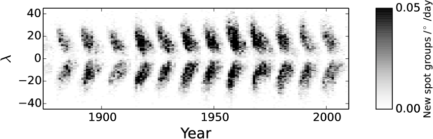
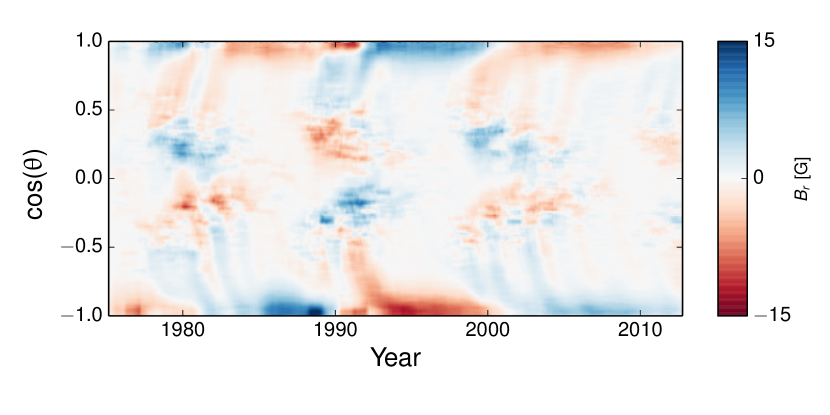
Observations of the type described in Section 2.2 are the constraints we have for the solar dynamo. They contain a lot of information, some of which can be summarized in simple figures, and some of which can be distilled into “laws”. Two figures which contain a lot of information are the butterfly diagram (Maunder, 1904, see also Figure 1) and the magnetic butterfly map (Figure 2).
From the observations a number of properties (some of them “laws”) have been described in the literature. A comprehensive solar dynamo model should be able consistent with these observational constraints. We begin with a number of constraints that are directly related to the magnetic activity.
11 year activity cycles, 22 year magnetic cycles.
A good proxy of magnetic activity is the number of sunspots, which varies in time with minima every 10 to 12 years. This was first noted by Schwabe (1849). Different cycles have different amplitudes (and modulation on longer periods might be present, e.g. Gleissberg, 1939). The 11 year solar activity cycle corresponds to half of the 22 year magnetic cycle (Hale et al., 1919), with the dominant polarity of the leading sunspots in each hemisphere changing between each activity cycle.
Spörer’s Law.
Hales law.
The magnetic nature of sunspots was discovered by Hale (1908). Sunspots typically appear in groups, with the leading and trailing spots (with respect to the solar rotation) having different polarities. The leading spots in each hemisphere mostly have the same polarity, and the polarity is opposite in the other hemisphere. The polarities of the leading and following spots switch between cycles (Hale et al., 1919).
Joy’s law.
As implied by Hales Law, sunspots often appear as bipolar pairs with the leading spots during one cycle and in one hemisphere having the same polarity. This is a statement about the east-west orientation of the sunspots. There is also a tendency for the leading spots to be slightly closer to the equator than the following spots. This tendency is much weaker than that of Hale’s law, with the angle implied by the North-South separation compared to the East-West separation being about 7 degrees. This effect is known as Joy’s law and was reported by Hale et al. (1919). There is some evidence that the strength of the effect depends on the strength of the cycle (Dasi-Espuig et al., 2010).
The effect is also much weaker in the sense that there is a lot of scatter in the North-South separation so that the effect is only robust when a large sample of sunspots is considered.
Waldmeier effect.
The Waldmeier effect states that strong cycles peak earlier than weak cycles (Waldmeier, 1941) (although the Waldmeier effect does not appear in all measures of the solar activity, cf Dikpati et al., 2008; Cameron and Schüssler, 2008). There is a closely related fact that strong cycles rise quickly, which Karak and Choudhuri (2011) call WE2, for the Waldmeier effect 2.
North-South asymmetry.
Extended cycle.
While the sunspot number has a period of around 11 years, the butterfly diagram indicates that the wings overlap so that sunspots corresponding to each cycle are present for about 13 years. Smaller than sunspots, ephemeral regions associated with a cycle have been shown to emerge about 5 years earlier, so the activity related to one cycle extends to about 18 years (Wilson et al., 1988).
Correlation between polar fields, open flux and strength of next cycle.
There is a strong correlation between the polar field at minimum (determined using polar faculae as a proxy) and the strength of the next cycle (Muñoz-Jaramillo et al., 2013); a stronger correlation exists between the Sun’s open flux, determined using the minima of the index as a proxy, and the strength of the next cycle (Wang and Sheeley, 2009). Cameron and Schüssler (2007) have suggested that this might be accounted for by the overlapping of cycles combined with the Waldmeier effect. A commonly claimed effect that the length of a minimum correlates positively with the weakness of the next cycle peak has been shown from sunspot data by (Dikpati et al., 2010a) to be false for the most recent 12 cycles.’
Magnetic fields at the surface are advected by surface flows as if they were corks.
Coronal Mass Ejections and magnetic helicity fluxes.
The structure of the magnetic field in the solar atmosphere, with filaments and sigmoid shaped active regions as well as the various types of activity in the solar atmosphere, such as flares and coronal mass ejections also contain information related to the solar cycle. The interpretation of these structures in terms of the helicity generated by the dynamo is however not straightforward (Zirker et al., 1997). We return to the helicity in some detail in Section 5.
Grand minima and maxima.
The above “laws” and properties of the magnetic activity are mainly based on the last few hundred years of data. We however know that the solar dynamo does not always behave like this – there are extended periods of low activity including the Maunder minimum (Spoerer, 1889b). They occur on average every 300 years (Usoskin et al., 2007) and presumably represent a different state of the dynamo. We have very few observational constraints for this state of the dynamo and therefore do not discuss it further in this paper.
3 Synthesising the observations and theory
We now turn to the open problem of synthesizing the observations and the “laws” they embody with well known basic physics in order to gain an understanding of the solar dynamo.
3.1 The omega and alpha effects
Cameron and Schüssler (2015) used the simplicity of the toroidal field implied by Hale’s law to show that the surface magnetic field plays a key role in the solar dynamo. The argument begins by noting that Hale’s law tells us that in each hemisphere, and during one cycle, the leading spots mainly (about 96% for large active regions, Wang and Sheeley, 1989) have the same magnetic polarity. This strong preference for the leading spots to have the same polarity indicates that the spots are coming from the emergence of toroidal flux that is all of the same polarity. The authors then considered the induction equation
| (1) |
where and are velocity and magnetic fields, is time, is the current density, is the magnetic permeability, and is the magnetic diffusivity with being the conductivity. They then applied Stokes theorem to with a contour in a meridional plane and encompassing the convection zone in the northern hemisphere. This allowed them to demonstrate that the generation of net toroidal flux in each hemisphere is dominated by the winding up of the poloidal flux threading the poles of the photosphere at the poles by the latitudinal differential rotation.
The polar fields themselves are the remnants of flux that has crossed the equator (Durrant et al., 2004), which is dominated by either the emergence of tilted active regions across the equator (Cameron et al., 2013) or the advection of active region flux across the equator due to the random shuffling of the field lines due to the supergranular flows.
The simplicity of the toroidal magnetic field at solar maxima, and the poloidal magnetic field at solar minima, therefore indicates that the solar dynamo is of the Babcock-Leighton type. Explicitly it is an alpha-omega dynamo where the relevant poloidal field threads through the photosphere. The omega effect is simply the winding up of this poloidal field by the latitudinal differential rotation. The alpha effect is what produces the tilt of the active regions with respect to the equator (Joy’s law).
We comment that the question of why we have a butterfly diagram, why sunspots obey Joy’s law, why the cycle length is around 11 years, and why sunspots only emerge below about 40 degrees all remain open questions. They are difficult to answer because they are intimately related to the subsurface dynamics, which are mostly poorly understood theoretically and observationally. In the next two subsections we discuss some of the ideas which are in the literature.
3.2 Equatorial migration of the butterfly wings.
Spörer’s law (discussed in Section 2.3.2) states that the latitude of emergence of sunspots propagates towards the equator as the cycle proceeds. The most straightforward (and probably correct) interpretation of this is that the underlying toroidal field is propagating towards the equator. There have been two main suggestions to explain the propagation of the toroidal field. The first is that of Parker (1955a), and explains the equatorward propagation in terms of a dynamo wave. The cause of the equatorial propagation in this model is explained in Figure 3 in the case of a Babcock-Leighton dynamo. The essential idea is that radial differential shear causes toroidal flux to propagate latitudinally. The direction of propagation (equatorwards or polewards) depends on the sign of the alpha effect (which generates poloidal flux from toroidal flux) and the on whether the differential rotation rate increases or decreases with depth (Yoshimura, 1975).
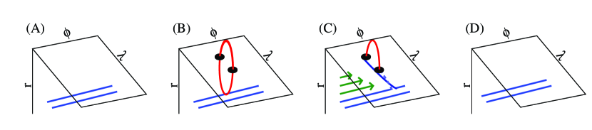
In terms of the Sun, the sign of the alpha effect is generally believed to be such that differential rotation has to increase with depth to obtain equatorward propagation. This is an issue on the Sun where the differential rotation decreases inwards near the base of the convection zone in the range of latitudes where sunspots form (Brown and Morrow, 1987). Thus if the solar dynamo is substantially located in the tachocline then this mechanism is excluded, the mechanism is however viable if the winding up of the toroidal field occurs in the near-surface shear layer.
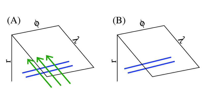
The second mechanism for explaining the equatorward propagation is shown in Figure 4 and is supposed to work at the base of the convection zone. The essential idea is that, if the meridional flow near the base of the tachocline is sufficiently strong, and if the latitudinal transport due to diffusion is sufficiently weak, then the simple advection of the toroidal flux by the meridional flow can produce the observed equatorial migration (Wang and Sheeley, 1991; Choudhuri et al., 1995; Durney, 1995; Dikpati and Charbonneau, 1999; Küker et al., 2001).
Which, if either, of these two explanations accounts for the transport on the Sun remains an open question.
3.3 Emergence latitudes
A second important question, which is probably closely related, is why sunspots overwhelmingly appear at latitudes below 40 degrees in latitude (see Figure 1). An obvious explanation for this would be that the toroidal flux is concentrated at low latitudes, however this explanation is problematic for Babcock-Leighton type dynamos where the latitudinal differential shear occurs over essentially all latitudes. A second possible mechanism considers the instability which leads to flux emergence. This explanation assumes that the toroidal flux is stored in or near the tachocline. In this case flux tubes must have a field strength of about G in order to have a substantial number of emergences at low latitude (Choudhuri and Gilman, 1987). The argument is that if the tubes are weaker then their rise is more affected by the Coriolis force which preferentially causes them to rise with at a constant distance from the rotation axis (i.e. along cylinders). The value of G is nicely consistent with the field strength required to produce Joy’s law (D’Silva and Choudhuri, 1993). Such flux tubes turn out to be much more unstable (Parker, 1955b) at low latitudes than at high latitudes (Caligari et al., 1995), hence if the toroidal flux is stored in the tachocline then even if the G loops form at high latitudes the loops are unable to escape to the surface.
This is an attractive possibility because the value of G links several observational results. However we caution that this effort was focussed on the case where the storage is in the tachocline or near the base of the convection zone because this was the dominant paradigm at the time the work was carried out. Much less work has been put into considering why sunspots don’t emerge at high latitudes in the case where the toroidal field is stored in the bulk of the convection zone. For this reason we regard the issue of the latitudinal range of the butterfly diagram as an open question.
3.4 Length of the solar cycle
It is somewhat sobering that after more than 160 years after the discovery by Schwabe (1849) that the level of solar activity varies with a period of about 11 years that we still don’t have a good idea of why it is 11 years.
In principle the length of the solar cycle should reflect the latitude range over which activity appears (say from a latitude of 30 degrees at the start of a cycle to 8 degrees at the end of a cycle) and the rate at which it propagates towards the equator. Within the framework of flux transport dynamos, the rate at which activity propagates towards the equator and the period of the dynamo, is largely determined by the meridional flow circulation rate (Dikpati and Charbonneau, 1999), however we have no clear basis in either observations or theory for understanding why the strength of the meridional flow at depth should be such that the dynamo period is 11 years. Within the alternative frame of a dynamo wave framework the period is set mainly by the magnitude of the alpha and omega effects, and the alpha effect in particular is not well understood.
To end this section on a positive light, it is clear that improving our understanding both what causes the equatorward propagation and what sets the latitudinal extent of the butterfly diagram, will give us a clearer handle on why the period of the solar cycle is 11 years.
3.5 The alpha effect
The above discussion indicates that the net toroidal field in each hemisphere is produced by the winding up of poloidal field by latitudinal differential rotation. In this regard it is only the field that threads through the surface which has an effect on the net flux. This winding up of the field is the omega effect of an alpha-omega dynamo. The details of how the alpha effect actually works in the Sun is less well understood – we observe the emergence of magnetic bipolar regions which are systematically tilted with respect to the equator, we observe their subsequent evolution, and we can infer (as in the previous section) that this is the field which is the poloidal field which gets wound up to produce the net toroidal flux in each hemisphere. What we do not observe are the processes which cause the field to emerge with a tilt.
It is relatively clear that the Coriolis force is implicated in the tilt; the uncertainty is whether the Coriolis for acts directly on the flows associated with the rise of the flux tube (e.g. D’Silva and Choudhuri, 1993), or whether it acts on the convective flows which then interacts with the flux tube (Parker, 1955a). This question is currently completely open.
Even without a proper understanding of the subsurface processes we can include flux emergence and Joy’s law into idealized mean-field simulations. Most of the recent work along these lines has been in the context of the flux transport dynamo, and the next section will outline some results from these efforts.
4 Modeling dynamo action
4.1 Flux-transport dynamos
Two-dimensional “flux-transport” dynamos incorporate in some form all of the processes discussed above, including the idea of flux emergence from toroidal flux at the base of the convection zone producing tilted active regions at the surface. These models have been successful in simulating the most important features of the solar cycle, including the butterfly diagram, polar field reversals near solar cycle maximum, certain global coronal features, and certain asymmetries between North and South hemispheres.
These models were used to simulate and predict the timing and amplitude of solar cycle 24 (Dikpati et al., 2006; Choudhuri et al., 2007; Dikpati et al., 2010b; Nandy et al., 2011), with limited success. There are several possibilities for this. Some of the suggestions of what was not included (but needs to be) are changes in the global meridional circulation profile and speed (Belucz and Dikpati, 2013), or localized inflow cells associated with active regions (Cameron and Schüssler, 2012; Shetye et al., 2015) or the scatter in tilt angles (Jiang et al., 2015). Unfortunately the results from helioseismology are too divergent to provide guidance on changes in the meridional flow (for example, compare the results in recent publications Ulrich, 2010; Zhao et al., 2013; Schad et al., 2013; Jackiewicz et al., 2015).
One possibility, supported by the observations, is that the weak cycle 24 is the result of the actual values of the tilt angles in cycle 23 (Jiang et al., 2015). The essential point here is that poloidal source term in the Babcock-Leighton model is based on Joy’s law, which is extremely noisy. The noise in Joy’s law translates to noise in the alpha effect, and thus to the strength of the different cycles. For cycle 23 Jiang et al. (2015) used the observed tilt angles (Li and Ulrich, 2012) and showed that alpha effect was indeed weak for cycle 23 (thus accounting for the weak cycle 24).
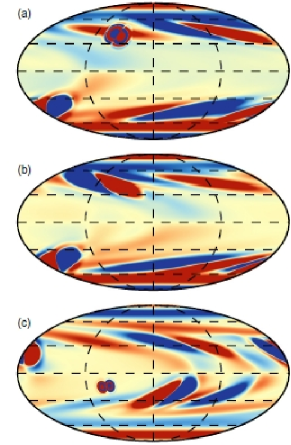
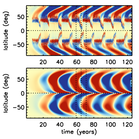
Current work includes extending the simulations to 3D, see, e.g., Miesch and Dikpati (2014). An example of such a simulation is shown in Figure 5, which depicts the longitude-latitude pattern of emerged flux, and the patterns of surface mean poloidal fields and deep-seated toroidal fields that are created in a sequence of solar cycles.
However, perhaps the biggest challenge to the flux-transport dynamos model is whether the meridional circulation is single-celled or multiple-celled or is indeed not steady at all. Many solar cycle features can be reproduced well by a flux-transport dynamo model if the meridional circulation contains a single cell in each hemisphere, but models with two cells in depth do not (Belucz et al., 2015). There is currently no consensus from observational evidence and meridional circulation models on the dominant profile of meridional flow in depth and latitude within the convection zone and tachocline. At the photosphere there is clearly one primary, poleward cell or often along with that a weak reverse cell appears at high latitudes. If it is established that there are two cells in depth, then another paradigm shift in solar dynamo theory will be needed; however it seems to be too early to decide on that issue now.
4.2 Global convective dynamo simulations
Attempts have also been made to simulate the convective motions and dynamo action in the Sun, with as few assumptions as possible – essentially from first principles. The first semi-successful attempts go back to the early 1980s when two different groups used the Cray 1 computer at the National Center for Atmospheric Research in Boulder (Colorado): Peter Gilman using a model of rotating convection (Gilman and Miller, 1981) and Meneguzzi et al. (1981) using forced turbulence in a Cartesian domain. Both studies provided remarkable first steps into numerical studies of large-scale and small-scale dynamos, but they also demonstrated that simulating the Sun will be difficult.
Subsequently, Gilman (1983) obtained cyclic solutions that were however quite different from the Sun: instead of equatorward migration of magnetic activity, he obtained poleward migration. Furthermore, small-scale dynamo action was not well understood at the time and the original paper by Meneguzzi et al. (1981) did not even quote the now important reference to the paper by Kazantsev (1968). The role of helicity was also not clear in some of those first studies, see also Kida et al. (1991). This was partly because those early simulations did not have sufficient scale separation, i.e., the scale separation ratio , where is the smallest wavenumber in the domain, was too small, as was noted subsequently (Haugen et al., 2004). In agreement with earlier work on rapidly rotating convection (Gilman, 1977), the contours of angular velocity tend to lie on cylinders. This implies that the radial gradient of the local angular velocity, , is positive. Therefore, as expected predictions from mean-field dynamo theory, the dynamo simulations of Gilman and Miller (1981) and Glatzmaier (1985) produced poleward migration, and were thus unable to reproduce the solar butterfly diagram. (These simulations were subsequently applied to the geodynamo problem by Glatzmaier and Roberts, 1995, where success was much clearer.)
From these simulations it is clear that reproducing the basic properties of the convection and the large-scale flows it drives are essential for a complete understanding of why a rotating middle-aged star such as the Sun should have an 11 year activity cycle and a butterfly diagram with equatorward propagation.
Computing power has increased dramatically since 1981, and simulations in more turbulent regimes became possible. This leads to flow patterns departing from otherwise nearly perfectly cylindrical contours (Miesch et al., 2000). Global simulations are now being conducted by many groups. Simulations with the anelastic spherical harmonic (ASH) code (Brun et al., 2004) work with a mean stratification close to that of mixing length theory, but at the solar rotation rate the resulting dynamo is statistically steady. Only at higher rotation rate, the solutions become time-dependent and cyclic (Brown et al., 2010). Simulations with the EULAG code (Ghizaru et al., 2010; Racine et al., 2011) also produce cyclic solutions, although the latitudinal migration of the mean magnetic field is weak. The pattern of meridional circulation in the simulations is, to date, mostly multicellular. This is in stark contrast to mean-field (flow) models, in which differential rotation is produced by the effect and meridional circulation is dominated by one large cell (Brandenburg et al., 1992). As mentioned above, helioseismology does not yet provide a consistent answer to guide the theory or simulations.
A (surprising) key issue which has emerged is the convective power spectrum. Observations through correlation tracking (Rieutord et al., 2008; Hathaway, 2012) and helioseismology (Hanasoge et al., 2012) suggest that the power in large-scale convective flows (giant cells) is very small. As alluded to in the introduction, the helioseismic evidence is contested (Greer et al., 2015), so the question remains open on the observational side. As already suggested by Spruit (1997), the structure of the large-scale convection is also unclear on the theoretical side – global simulations miss the physics of the radiating surface, and this may turn out to be crucial for producing simulations with realistic flow structures, which may be dominated by what is known as ‘entropy rain’. This would be a fast small-scale downflow originating from the surface in such a way that the bulk of the convection zone is nearly isentropic, but with a slightly stable stratification so as not to produce giant cell convection in the deeper parts (Brandenburg, 2015). Clearly, simulations must eventually be able to reproduce the Sun, and reproducing the convective power spectrum and the large-scale flows is probably a precondition to accurately reproducing the solar dynamo. Knowing what those flows are is essential.
Currently the convective simulations are most useful in providing guidance on what is possible, and elucidating mechanisms. For example in simulations by Käpylä et al. (2012) using the Pencil Code111https://github.com/pencil-code. , there was pronounced equatorward migration, which was later identified as being due to a local negative radial gradient (Warnecke et al., 2014). While this is a feature not expected to be present in the Sun, it does demonstrate that the dynamo wave in global simulations follows closely that expected from mean-field simulations (Parker, 1955a; Yoshimura, 1975). Global simulations have also produced evidence for strong () flux tubes in the bulk of the convection zone (Nelson et al., 2014; Fan and Fang, 2014). This is interesting in view of understanding the overall magnetic flux concentration required to form active regions, although further amplification is needed; see Stein and Nordlund (2012) and Mitra et al. (2014) for possible mechanisms.
Both flux transport and full 3D dynamo models necessarily contain parametrizations of processes acting on scales smaller than spatially resolved. These parametrizations are all rooted in formulations of MHD turbulence, in which helicity of velocities, magnetic fields and electric currents play central roles. Therefore we consider helicity effects in detail in section 5
5 The roles of magnetic helicity
As revealed above, we are still struggling to understand the true nature of the solar dynamo and the relation between the large-scale dynamo in the Sun and in global simulations. In this regard we need to be sure that what we see in the simulations survives in the limit of large magnetic Reynolds numbers such as are found in the Sun. This has not been yet been fully confirmed. One example of this is that in the simulations the large-scale field magnetic field (as opposed to the small-field magnetic field) is often found to decrease with increasing values of . In this section we show that this can be understood quantitatively in terms of magnetic helicity conservation, as will be discussed below.
Magnetic helicity is a conserved quantity in ideal MHD, and as such is conserved in the absence of microphysical diffusivity (i.e. it is not changed by the turbulent flow, or the associated turbulent magnetic diffusivity). In a closed volume, at low microphysical diffusivity of the sun, the amount of helicity is not expected to change on timescales of the solar cycle. This is remarkable and unprecedented in hydrodynamic turbulence. The only way that magnetic helicity can change and evolve (e.g., over the course of the 11 year cycle) is through magnetic helicity fluxes. They can be determined at the surface and this allows contact to be made between theory and observations. In this section we will therefore outline some of the different attempts to determine the helicity flux through the solar surface and what this tells us about the solar dynamo.
There are other types of helicity, including kinetic helicity, which also play important roles in dynamo theory. Most importantly kinetic helicity makes it relatively simple to generate a large-scale magnetic field (Moffatt, 1969). We therefore begin by discussing the different types of helicity and their definitions.
5.1 Definitions.
Mathematically, helicities are so-called pseudo-scalars, i.e., they are the dot product of a proper vector and an axial vector. (The latter changes its orientation when viewed in a mirror.)
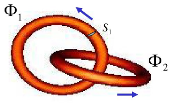
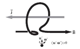
Four such pseudoscalars are of particular interest: mean kinetic helicity density , with being the vorticity, mean magnetic helicity density , with being magnetic vector potential such that , mean current helicity density , and finally the cross helicity, ; see Yokoi (2013) for a recent review, especially on cross helicity. All these helicities have topological interpretations that refer to the mutual linkage between interlocked structures, for example two flux rings in the case of magnetic helicity (Fig. 6, left), two vortex rings in the case of kinetic helicity, two current tubes in the case of current helicity, and a vortex tube with a magnetic flux tube in the case of cross helicity. This topological interpretation goes back to early work of Moffatt (1969) and is important for the existence of qualitative helicity indicators.
Qualitative helicity indicators.
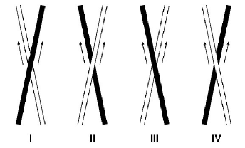
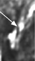
Familiar to all of us is the case of kinetic helicity in the Earth’s atmosphere: a glance at weather maps in England and Australia shows low pressure whirlpools of opposite orientation. This helicity is the direct result of the Coriolis force acting on large-scale flows. Likewise the Sun is rotating and has large-scale (supergranulation or larger) flows which feel the effect of the Coriolis force. Hence on the Sun we see the morphological or qualitative signatures of helicity in large-scale structures: H images reveal S-shaped structures in the south and N-shaped structures in the north (i.e., inverted S-shaped structures). They are referred to as sigmoidal structures and the importance of interpreting them was recognized by Sara Martin (1998a, b) and many people after her (Canfield et al., 1999; Magara and Longcope, 2001; Gibson et al., 2002). These helicity indicators can also be linked to mutual crossings of magnetic flux structures, which are best seen at EUV wavelengths where filaments appear occasionally in emission. This technique, which is due to Chae (2000), requires an additional assumption: the angle between two adjacent structures is an acute one (i.e., the invisible arrows of the field vectors point in roughly the same direction) rather than an obtuse one, as illustrated by the configurations I–IV in Fig. 6 from his paper. His study confirms that the magnetic field has negative helicity in the north (corresponding to crossings of types III and IV with N-shaped or so-called dextral filaments) and positive helicity in the south (corresponding to crossings of types I and II with S-shaped or so-called sinistral filaments). In Fig. 6 we also reproduce an EUV image from his paper with a filament of type III in the northern hemisphere, consistent with negative helicity.
Semiquantitative indicators.
We turn now to semiquantitative indicators, by which we mean quantitative measures of something which is only qualitatively linked the helicity. As an important example, we can consider the product of what is known as the horizontal divergence and horizontal curl of the velocity, defined respectively as
| (2) | |||
| (3) |
Here, commas denote partial differentiation. The horizontal curl is just the same as the component of the usual curl. The product of and has been determined for the Sun using local correlation tracking and local helioseismology by Langfellner et al. (2014). In fact, Rüdiger et al. (1999) have shown that the product of and is a proxy of kinetic helicity. This is simply because one of the three terms in is , but, using the anelastic approximation, , where is density, and the definition of the density scale height,
| (4) |
we have and therefore .
Quantitative helicity measures.
The measurement of current helicity density, , goes back to early work of Seehafer (1990), who determined from circular polarization measurements, while and (giving ) were obtained from linear polarization. Such measurements are now obtained routinely from solar vector magnetograms. They all suggest that is negative in the north and positive in the south. Typical values of are around (Zhang et al., 2014).
Regarding magnetic helicity, there is a notable complication in that is gauge-dependent and changes by adding an arbitrary gradient term to , which does not change . Exceptions are triply-periodic and infinite domains, for which turns out to be gauge-invariant. However, there exists a quantity called the relative magnetic helicity
| (5) |
where is a potential field () that satisfies (Berger and Field, 1984). It is gauge-independent, but it can only be determined over a finite volume. There is also a corresponding magnetic helicity flux , where is the electric field. Simple examples of magnetic helicity and its flux have been presented by Berger and Ruzmaikin (2000) for theoretical models with rigid and differential rotation as well as with an assumed effect. Quantitative measurements for the Sun’s magnetic field are in the range of (DeVore, 2000; Chae, 2001; Welsch and Longcope, 2003). This value is easily motivated by standard dynamo theory (Brandenburg, 2009).
Let us finally comment on the cross helicity density , or its spatial average . Just like , it is a quantity that is conserved by the nonlinear interactions of the magnetohydrodynamic equations (Woltjer, 1958), but it is often small, i.e., the normalized cross helicity , which is the ratio of two conserved quantities (the latter being the total energy), is far away from its extrema of and , if it was vanishing initially. An exception is a stratified layer with an aligned magnetic field. This also applies to the solar wind, where there can be regions where gravity and the magnetic field are systematically aligned with each other. In those cases, a finite cross helicity can be driven away from zero. This can be understood by noting that there are two externally imposed vectors: gravity with a parallel (vertical) magnetic field . The latter is a pseudovector, giving rise to a pseudoscalar that is odd in the magnetic field—just like . Indeed, theoretical and numerical work by Rüdiger et al. (2011) showed that
| (6) |
where denotes the fluctuating magnetic field, is the correlation time of the turbulence, is its rms velocity, is the sound speed, is the turbulent magnetic diffusivity, and is the density scale height defined in Eq. (4) for an isothermal layer. Measurements for active regions are in the range – (Zhao et al., 2011; Rüdiger et al., 2012).
5.1.1 Large and small length scales
The length-scale dependence of the different types of helicity can be investigated by looking at the spectra of magnetic energy and helicity.
Magnetic helicity spectra.
Given that the magnetic helicity is a conserved quantity, it should be zero if it was zero initially. However, because it is a signed quantity, “zero” can consist of a “mixture” of pluses and minuses. These two signs can be segregated spatially (typically into north and south) as well as spectrally (into large and small scales). This is discussed in more detail below when we talk about catastrophic quenching of a large-scale dynamo. For now it suffices to say that we can define a magnetic helicity spectrum , where is its wavenumber (inverse length scale), and whose integral gives the mean magnetic helicity density, i.e.,
| (7) |
If the turbulence or the magnetic field were homogeneous, it can be related to the Fourier transform of the two-point correlation function
| (8) |
which is independent of owing to the assumption of homogeneity, and is the separation. Its Fourier transform over gives , which, under isotropy, has the representation
| (9) |
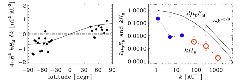
where is the unit vector of and is the magnetic energy spectrum with the normalization . The dependence of and on the modulus of the wavevector is again an consequence of isotropy. This relation is slightly modified when applied to the two-dimensional solar surface, but it allows us to obtain for the first time spectra of magnetic helicity, i.e., information about its composition from different length scales; see Zhang et al. (2014) for results that have confirmed that, in the southern hemisphere, the magnetic helicity is positive on wavenumbers of about . This is in agreement with the results presented in Sect. 3.5.
Magnetic helicity spectra of the solar wind.
A similar technique to that presented above has been applied to the solar wind, where it is possible to obtain the magnetic field vector from in situ spacecraft measurements. The idea to compute the magnetic helicity spectrum by using Eq. (9) goes back to early work of Matthaeus et al. (1982), who used data from Voyager 1 and 2. To obtain measurements at positions and , one uses the Taylor hypothesis to relate the spatial separation to a temporal separation through , where is the solar wind velocity of about and is some reference position. However, since Voyager 1 and 2 flew close to the equatorial plane, the resulting magnetic helicity was expected to fluctuate around zero, which was indeed the case. This changed when data from Ulysses were used for such an analysis (Brandenburg et al., 2011b). In Fig. 7 we show the resulting spectrum, as well as the latitudinal dependence a specific . We should point out that is here gauge-invariant because we are dealing with an infinite or periodic domain, which is automatically implied by the use of Fourier spectra. Note also that , which is also known as the realizability condition.
The importance of magnetic helicity became particularly clear in connection with understanding the phenomenon of catastrophic quenching, which will be explained in the next section.
5.1.2 Magnetic helicity conservation
To understand the basics of dynamo action, including saturation mechanisms, it is often useful to work in idealized periodic geometries, and with turbulence either from simple forcing or driven by convection. While early work in this context at small values of were promising (Brandenburg et al., 1990), subsequent studies at larger values of showed that the field-aligned emf, approaches zero as (see Cattaneo and Hughes, 1996).
This was understood as a consequence of magnetic helicity conservation (Gruzinov and Diamond, 1996). Consider the equation for the fluctuation of the magnetic vector potential , where angle brackets denote volume averages and lower case symbols the fluctuations. The mean flow is assumed to vanish. Thus, we have
| (10) |
We now derive the equation for the mean magnetic helicity density of the small-scale field as
| (11) |
In the steady state, we find that
| (12) |
This relation for “” is sometimes known as Keinigs relation (Keinigs, 1983) and shows not only that “” is positive when is negative (i.e., in the north), but also that “” when , i.e., in the limit of large magnetic Reynolds numbers. This remarkable result seems like a disappointment to effect theory, but it only means that no , defined as a volume average (!), can be generated. This should then be no surprise, because the volume average of is a conserved quantity for the periodic boundary conditions used in the study of Cattaneo and Hughes (1996) (which is the reason we put in quotes).
In reality, we are interested in averages that vary in space.
When we consider the case where the averages are allowed to vary in space, the divergences of magnetic helicity flux will in general be non zero in the magnetic helicity equation.
Dynamical quenching.
Consider planar averages, denoted by an overbar, magnetic helicity conservation yields instead
| (13) |
Here, is the magnetic helicity flux from the fluctuating magnetic field and is the kinetic effect, which itself could depend on , but this is here neglected. The main contribution to the quenching in Eq. (13) comes from the magnetic contribution to the effect, where (Pouquet et al., 1976).
Equation (13) confirms first of all that is catastrophically quenched (i.e., in an -dependent fashion), when volume averages are used, i.e., when and the assumption of stationarity is made (). In that case, we obtain
| (14) |
This equation was first motivated by Vainshtein and Cattaneo (1992) on the grounds that the energy ratio of small-scale to large-scale magnetic fields is proportional to , i.e., (e.g. Moffatt, 1978; Krause and Rädler, 1980), but this relation becomes invalid at large values of where the rhs has to be replaced by (Kleeorin and Rogachevskii, 1994). Furthermore, this relation assumes that the small-scale magnetic field is solely the result of tangling, so dynamo action is actually ignored in the old argument of Vainshtein and Cattaneo (1992).
It is now clear from Eq. (13) that catastrophic quenching is alleviated when there are mean currents (), which is already the case in triply-periodic helical turbulence, where, in fact, a super-equipartition field with can be generated, albeit only on a resistive time scale (Brandenburg, 2001). Here, is the aforementioned scale separation ratio. Nevertheless, because of the long saturation time (which is determined by the microphysical diffusivity), such dynamos cannot be astrophysically relevant.
The ultimate rescue from catastrophic quenching seems to come from the presence of magnetic helicity flux divergences (). Interestingly, what is primarily required is that the dynamo-generated field is no longer completely homogeneous as in dynamos, where is a Beltrami field with spatially constant . For example, when there is shear, we can have -type dynamo action with finite within an otherwise periodic (or shearing-periodic) domain where catastrophic quenching was indeed found to be alleviated (Hubbard and Brandenburg, 2012). However, to demonstrate complete independence is still difficult, and can only be expected for (Del Sordo et al., 2013).
At this point it is useful to return to the question of gauge-dependence. The evolution equation for the mean magnetic helicity density of the fluctuating field, , can be written with a finite magnetic helicity flux divergence,
| (15) |
On can now examine whether , in the gauge under consideration, happens to be statistically stationary. In general, this does not need to be the case (for an example, see Fig. 2 of Brandenburg et al., 2002), but if it is, we can consider the overbars as denoting also an average over time, because then the left-hand side of Eq. (15) vanishes and we have
| (16) |
What is remarkable here is the fact that, at least in this special case ( constant in time) the magnetic helicity flux divergence is no longer gauge-dependent, i.e., it must be the same in all gauges. Moreover, unlike the aforementioned surface-integrated gauge-invariant magnetic helicity flux , we can now make statements about its local dependence and its physical relation to mean flows and gradients of the magnetic helicity density. This has been done in several simulations which all confirm that an important part of the magnetic helicity flux is carried turbulent-diffusively like in Fickian diffusion (Mitra et al., 2010; Hubbard and Brandenburg, 2010; Del Sordo et al., 2013).
5.1.3 Observational clues
The sign of the helicity at different spatial scales.
To make contact with solar magnetic helicity observations, we must ask about the scales on which helical fields are generated. If the large-scale field is really generated by an effect, then both magnetic and current helicities of the large-scale field should have the same sign (Brandenburg, 2001; Blackman and Brandenburg, 2002) and should be positive in the north, where . On large scales, the magnetic helicity obeys
| (17) |
where we have assumed an isotropic effect and an isotropic turbulent magnetic diffusivity and is the total (turbulent plus microphysical) magnetic diffusivity. Note that, in the steady-state, we have
| (18) |
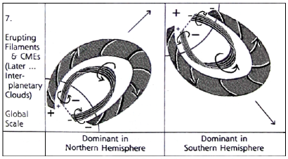
i.e., the magnetic helicity of the large-scale field should indeed be positive in the north. At small scales, on the other hand, we expect the opposite sign. Only the latter has been observed directly. However, the N- and S-shaped structures in H images can indirectly be associated with large-scale fields resulting from a positive affect in the north; see Fig. 8. Indeed, the barbs of filaments are an example, because right-handed (left-handed) barbs are found in filaments in which the purely axial threads (independent of the barb threads) have a slight but definite shape of a left-handed (right-handed) sigmoid. This way of interpreting the two signs of helicity within a single filament was discussed by Ruzmaikin et al. (2003); see Table 1 of (Martin, 2003) for details.
Helicity reversals within the solar wind.
The observation of the magnetic helicity spectrum in the solar wind poses some questions, because the sign is exactly opposite of what is observed at the solar surface. Theoretical support for this surprising result comes from simulations of dynamos with an extended outer layer that only supports turbulent diffusion, but no effect. A magnetic helicity reversal was first recognized in the simulations of Warnecke et al. (2011, 2012), but such reversals were already present in early mean-field simulations of Brandenburg et al. (2009), which included the physics of turbulent-diffusive magnetic helicity fluxes.
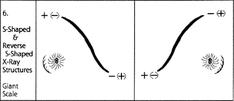
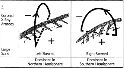
Two related explanations have been proposed. Firstly, within the dynamo the effects of and nearly balance, which implies that both terms enter the magnetic helicity equation with opposite signs; see Eq. (17). However, within the wind, the effect is basically absent, creating therefore an imbalance and thus a contribution of opposite sign. A related explanation assumes a steady state and invokes a turbulent-diffusive magnetic helicity flux obeying a Fickian diffusion law, i.e., , where is a turbulent diffusivity for magnetic helicity of the small-scale field. The difference from heat diffusion is that temperature is positive definite, but magnetic helicity is not. To transport positive magnetic helicity outward, we need a negative magnetic helicity gradient, which tends to drive it to (and even through) zero, which could explain the reversal. At present it is unclear which, if any, of these proposals is applicable. It is interesting to note, however, that similar reversals are seen also in the opposite orientations of coronal X-ray arcades in the northern and southern hemispheres; see Fig. 9. In essence, many filaments develop a sideways rolling motion that begins from the top down (Martin, 2003) and evidence of this motion was found in H Doppler observations and in 304 Angstroms images from SOHO (Panasenco and Martin, 2008) and subsequently in 304 Angstroms from SDO and STEREO (Panasenco et al., 2011). The most convincing evidence that the forces for this change come from the coronal environment is the correlation with coronal holes. Quiescent filaments without exception were found to roll from the top down away from adjacent coronal holes (Panasenco et al., 2013). The right-hand part of Fig. 9 shows the direction of motions in the filament that result in their becoming twisted during eruption. The general direction of the magnetic field is denoted by the polarity at the footpoints.
Magnetic structures from cross helicity?
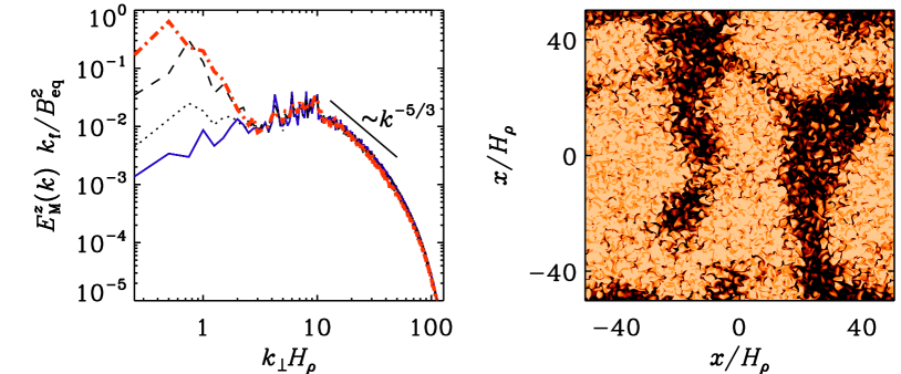
In the presence of strong stratification, cross helicity is being generated if a large-scale magnetic field pierces the surface. This leads to a gradual evolution of the magnetic energy spectra of the vertical field, , showing a growth at small wavenumbers, akin to inverse transfer resulting from the effect and approximate magnetic helicity conservation. This growth is associated with the development of magnetic structures; see Fig. 10.
The formation of such magnetic structures has also been associated with the possibility of a large-scale instability resulting from a negative contribution to the effective (turbulent) magnetic pressure. This instability is therefore referred to as negative effective magnetic pressure instability (NEMPI). Earlier work on NEMPI has shown a remarkably degree of predictive power of this theory in comparison with simulations (Brandenburg et al., 2011a; Kemel et al., 2013; Losada et al., 2013), but it is still unclear what drives the magnetic structures in simulations where the field strongly exceeds equipartition with the energy density of the turbulent motions (Mitra et al., 2014). Whether or not NEMPI or similar phenomena play a role in the formation of active regions or even sunspots is however an open question.
6 Conclusion
The question appears simple: Why does a star such as the Sun support have a global-scale magnetic field which reverses every 11 years and has equatorially propagating activity wings? We do not have anything like a complete answer to this question.
At the most fundamental level we do not we do not know the profiles of all the large-scale flows that are present. Beginning with convection, which is the driver for the global-scale motions and the magnetic field, we have to leave the reader with the following unanswered questions: Why is there so little power at scales larger than supergranulation in the solar photosphere (Lord et al., 2014)? Does this lack of power reflect a lack of power in these large scales at depth (compare the results in Hanasoge et al., 2012; Greer et al., 2015)? Is our fundamental picture of convection inapplicable to the solar convection zone (Spruit, 1997; Brandenburg, 2015)?
Moving to the flows on the global scale: What does the meridional circulation look like beneath the solar surface (Zhao et al., 2013; Schad et al., 2013; Jackiewicz et al., 2015)? What maintains the solar differential rotation? What maintains the meridional circulation? For the latter two questions we have some ideas (which give different answers), but they depend partly on the strength of the convective flows and will also depend on how the ’small-scale’ turbulent dynamo, supposed to operate in the convection zone, modifies the flows.
These problems in our understanding, for example the power spectrum of the convective flows in the Sun, are not necessarily critical for understanding the solar dynamo if we take the observed flows as given. This simplifies the problem to asking how the (partially) observed flows produce the solar dynamo with all its observed features. Even this more limited problem is not solved. In this review we have briefly highlighted two important open questions. One of these questions is: Why do sunspots only appear at latitudes below about ? The commonly given answer concerns the stability of toroidal flux located at the base of the convection zone, which for G flux tubes are much more unstable at low latitudes than at high latitudes. Little consideration has however been given in this regard to the possibility that the toroidal flux is stored in the bulk of the convection zone. The second question we have highlighted is what causes the equatorial propagation of the activity belt towards the equator, and here we have competing answers. Both of these problems appear to be difficult, and their solution is likely to come from improvements in helioseismology and modeling efforts.
In order to end on a bright note, we think it is important to point out some of the recent progress which has occurred. For example we have Hale’s law which tells us that the structure of the toroidal flux is quite simple, and at solar minimum the surface radial field is also simple (it is mainly near the poles and mainly of one sign in each hemisphere). This simplicity has enabled some rather strong conclusions to be drawn: the solar dynamo is an alpha-omega dynamo of the Babcock-Leighton type (Cameron and Schüssler, 2015). Furthermore we have a number of ideas as to why the amount of activity varies from cycle to cycle (e.g. Jiang et al., 2015), and critically we are beginning to test these models against real data (Dikpati et al., 2006; Choudhuri et al., 2007; Dikpati et al., 2010b; Nandy et al., 2011). We thus have a long way to go but are making progress and have the right tools and perspective to make real progress in the coming years.
Acknowledgements.
This work was, in part, carried out in the context of Deutsche Forschungsgemeinschaft SFB 963 “Astrophysical Flow Instabilities and Turbulence” (Project A16). This work was supported in part by the Swedish Research Council grants No. 621-2011-5076 and 2012-5797, as well as the Research Council of Norway under the FRINATEK grant 231444. This work has been partially supported by NASA grant NNX08AQ34G. The National Center for Atmospheric Research is sponsored by the National Science Foundation. NSO/Kitt Peak data used here are produced cooperatively by NSF/NOAO, NASA/GSFC, and NOAA/SEL. This work utilizes SOLIS data obtained by the NSO Integrated Synoptic Program (NISP), managed by the National Solar Observatory, which is operated by the Association of Universities for Research in Astronomy (AURA), Inc. under a cooperative agreement with the National Science Foundation. The synoptic magnetograms were downloaded from the NSO digital library, http://diglib.nso.edu/ftp.html We acknowledge the support from ISSI Bern, for her participation in the ISSI workshop on.References
- Arlt et al. (2013) R. Arlt, R. Leussu, N. Giese, K. Mursula, I.G. Usoskin, Sunspot positions and sizes for 1825-1867 from the observations by Samuel Heinrich Schwabe. Mon. Not. Roy. Astron. Soc. 433, 3165–3172 (2013). doi:10.1093/mnras/stt961
- Babcock (1961) H.W. Babcock, The Topology of the Sun’s Magnetic Field and the 22-YEAR Cycle. Astrophys. J. 133, 572 (1961). doi:10.1086/147060
- Balmaceda et al. (2009) L.A. Balmaceda, S.K. Solanki, N.A. Krivova, S. Foster, A homogeneous database of sunspot areas covering more than 130 years. Journal of Geophysical Research (Space Physics) 114, 7104 (2009). doi:10.1029/2009JA014299
- Belucz and Dikpati (2013) B. Belucz, M. Dikpati, Role of Asymmetric Meridional Circulation in Producing North-South Asymmetry in a Solar Cycle Dynamo Model. Astrophys. J. 779, 4 (2013). doi:10.1088/0004-637X/779/1/4
- Belucz et al. (2015) B. Belucz, M. Dikpati, E. Forgács-Dajka, A babcock–leighton solar dynamo model with multi-cellular meridional circulation in advection- and diffusion-dominated regimes. Astrophys. J. 806, 169 (2015). doi:10.1088/0004-637X/806/2/169
- Berger and Field (1984) M.A. Berger, G.B. Field, The topological properties of magnetic helicity. Journal of Fluid Mechanics 147, 133–148 (1984). doi:10.1017/S0022112084002019
- Berger and Ruzmaikin (2000) M.A. Berger, A. Ruzmaikin, Rate of helicity production by solar rotation. J. Geophys. Res. 105, 10481–10490 (2000). doi:10.1029/1999JA900392
- Bertello et al. (2010) L. Bertello, R.K. Ulrich, J.E. Boyden, The Mount Wilson Ca ii K Plage Index Time Series. Solar Phys. 264, 31–44 (2010). doi:10.1007/s11207-010-9570-z
- Blackman and Brandenburg (2002) E.G. Blackman, A. Brandenburg, Dynamic Nonlinearity in Large-Scale Dynamos with Shear. Astrophys. J. 579, 359–373 (2002). doi:10.1086/342705
- Brandenburg (2001) A. Brandenburg, The Inverse Cascade and Nonlinear Alpha-Effect in Simulations of Isotropic Helical Hydromagnetic Turbulence. Astrophys. J. 550, 824–840 (2001). doi:10.1086/319783
- Brandenburg (2009) A. Brandenburg, The critical role of magnetic helicity in astrophysical large-scale dynamos. Plasma Physics and Controlled Fusion 51(12), 124043 (2009). doi:10.1088/0741-3335/51/12/124043
- Brandenburg (2015) A. Brandenburg, Stellar mixing length theory with entropy rain. arXiv:1504.03189 (2015)
- Brandenburg et al. (2009) A. Brandenburg, S. Candelaresi, P. Chatterjee, Small-scale magnetic helicity losses from a mean-field dynamo. Mon. Not. Roy. Astron. Soc. 398, 1414–1422 (2009). doi:10.1111/j.1365-2966.2009.15188.x
- Brandenburg et al. (2002) A. Brandenburg, W. Dobler, K. Subramanian, Magnetic helicity in stellar dynamos: new numerical experiments. Astronomische Nachrichten 323, 99–122 (2002). doi:10.1002/1521-3994(200207)323:2¡99::AID-ASNA99¿3.0.CO;2-B
- Brandenburg et al. (1992) A. Brandenburg, D. Moss, I. Tuominen, Stratification and thermodynamics in mean-field dynamos. Astron. Astrophys. 265, 328–344 (1992)
- Brandenburg et al. (1990) A. Brandenburg, A. Nordlund, P. Pulkkinen, R.F. Stein, I. Tuominen, 3-D simulation of turbulent cyclonic magneto-convection. Astron. Astrophys. 232, 277–291 (1990)
- Brandenburg et al. (2011a) A. Brandenburg, K. Kemel, N. Kleeorin, D. Mitra, I. Rogachevskii, Detection of Negative Effective Magnetic Pressure Instability in Turbulence Simulations. Astrophys. J. Lett. 740, 50 (2011a). doi:10.1088/2041-8205/740/2/L50
- Brandenburg et al. (2011b) A. Brandenburg, K. Subramanian, A. Balogh, M.L. Goldstein, Scale Dependence of Magnetic Helicity in the Solar Wind. Astrophys. J. 734, 9 (2011b). doi:10.1088/0004-637X/734/1/9
- Brandenburg et al. (2014) A. Brandenburg, O. Gressel, S. Jabbari, N. Kleeorin, I. Rogachevskii, Mean-field and direct numerical simulations of magnetic flux concentrations from vertical field. Astron. Astrophys. 562, 53 (2014). doi:10.1051/0004-6361/201322681
- Brown et al. (2010) B.P. Brown, M.K. Browning, A.S. Brun, M.S. Miesch, J. Toomre, Persistent Magnetic Wreaths in a Rapidly Rotating Sun. Astrophys. J. 711, 424–438 (2010). doi:10.1088/0004-637X/711/1/424
- Brown and Morrow (1987) T.M. Brown, C.A. Morrow, Depth and latitude dependence of solar rotation. Astrophys. J. Lett. 314, 21–26 (1987). doi:10.1086/184843
- Brun et al. (2004) A.S. Brun, M.S. Miesch, J. Toomre, Global-Scale Turbulent Convection and Magnetic Dynamo Action in the Solar Envelope. Astrophys. J. 614, 1073–1098 (2004). doi:10.1086/423835
- Caligari et al. (1995) P. Caligari, F. Moreno-Insertis, M. Schussler, Emerging flux tubes in the solar convection zone. 1: Asymmetry, tilt, and emergence latitude. Astrophys. J. 441, 886–902 (1995). doi:10.1086/175410
- Cameron and Schüssler (2007) R. Cameron, M. Schüssler, Solar Cycle Prediction Using Precursors and Flux Transport Models. Astrophys. J. 659, 801–811 (2007). doi:10.1086/512049
- Cameron and Schüssler (2008) R. Cameron, M. Schüssler, A Robust Correlation between Growth Rate and Amplitude of Solar Cycles: Consequences for Prediction Methods. Astrophys. J. 685, 1291–1296 (2008). doi:10.1086/591079
- Cameron and Schüssler (2015) R. Cameron, M. Schüssler, The crucial role of surface magnetic fields for the solar dynamo. Science 347, 1333–1335 (2015). doi:10.1126/science.1261470
- Cameron and Schüssler (2012) R.H. Cameron, M. Schüssler, Are the strengths of solar cycles determined by converging flows towards the activity belts? Astron. Astrophys. 548, 57 (2012). doi:10.1051/0004-6361/201219914
- Cameron et al. (2013) R.H. Cameron, M. Dasi-Espuig, J. Jiang, E. Işık, D. Schmitt, M. Schüssler, Limits to solar cycle predictability: Cross-equatorial flux plumes. Astron. Astrophys. 557, 141 (2013). doi:10.1051/0004-6361/201321981
- Canfield et al. (1999) R.C. Canfield, H.S. Hudson, D.E. McKenzie, Sigmoidal morphology and eruptive solar activity. Geophys. Res. Lett. 26, 627–630 (1999). doi:10.1029/1999GL900105
- Carbonell et al. (1993) M. Carbonell, R. Oliver, J.L. Ballester, On the asymmetry of solar activity. Astron. Astrophys. 274, 497 (1993)
- Carrington (1858) R.C. Carrington, On the Distribution of the Solar Spots in Latitudes since the Beginning of the Year 1854, with a Map. Mon. Not. Roy. Astron. Soc. 19, 1–3 (1858)
- Cattaneo and Hughes (1996) F. Cattaneo, D.W. Hughes, Nonlinear saturation of the turbulent effect. PhRvE 54, 4532 (1996). doi:10.1103/PhysRevE.54.R4532
- Chae (2000) J. Chae, The Magnetic Helicity Sign of Filament Chirality. Astrophys. J. Lett. 540, 115–118 (2000). doi:10.1086/312880
- Chae (2001) J. Chae, Observational Determination of the Rate of Magnetic Helicity Transport through the Solar Surface via the Horizontal Motion of Field Line Footpoints. Astrophys. J. Lett. 560, 95–98 (2001). doi:10.1086/324173
- Chandrasekhar (1956) S. Chandrasekhar, Effect of Internal Motions on the Decay of a Magnetic Field in a Fluid Conductor. Astrophys. J. 124, 244 (1956). doi:10.1086/146218
- Cheung et al. (2010) M.C.M. Cheung, M. Rempel, A.M. Title, M. Schüssler, Simulation of the Formation of a Solar Active Region. Astrophys. J. 720, 233–244 (2010). doi:10.1088/0004-637X/720/1/233
- Choudhuri and Gilman (1987) A.R. Choudhuri, P.A. Gilman, The influence of the Coriolis force on flux tubes rising through the solar convection zone. Astrophys. J. 316, 788–800 (1987). doi:10.1086/165243
- Choudhuri et al. (2007) A.R. Choudhuri, P. Chatterjee, J. Jiang, Predicting Solar Cycle 24 With a Solar Dynamo Model. Physical Review Letters 98(13), 131103 (2007). doi:10.1103/PhysRevLett.98.131103
- Choudhuri et al. (1995) A.R. Choudhuri, M. Schussler, M. Dikpati, The solar dynamo with meridional circulation. Astron. Astrophys. 303, 29 (1995)
- Clette et al. (2014) F. Clette, L. Svalgaard, J.M. Vaquero, E.W. Cliver, Revisiting the Sunspot Number. A 400-Year Perspective on the Solar Cycle. Space Sci. Rev. 186, 35–103 (2014). doi:10.1007/s11214-014-0074-2
- Dasi-Espuig et al. (2010) M. Dasi-Espuig, S.K. Solanki, N.A. Krivova, R. Cameron, T. Peñuela, Sunspot group tilt angles and the strength of the solar cycle. Astron. Astrophys. 518, 7 (2010). doi:10.1051/0004-6361/201014301
- Del Sordo et al. (2013) F. Del Sordo, G. Guerrero, A. Brandenburg, Turbulent dynamos with advective magnetic helicity flux. Mon. Not. Roy. Astron. Soc. 429, 1686–1694 (2013). doi:10.1093/mnras/sts398
- DeVore (2000) C.R. DeVore, Magnetic Helicity Generation by Solar Differential Rotation. Astrophys. J. 539, 944–953 (2000). doi:10.1086/309274
- DeVore et al. (1984) C.R. DeVore, J.P. Boris, N.R. Sheeley Jr., The concentration of the large-scale solar magnetic field by a meridional surface flow. Solar Phys. 92, 1–14 (1984). doi:10.1007/BF00157230
- Diercke et al. (2015) A. Diercke, R. Arlt, C. Denker, Digitization of sunspot drawings by Spörer made in 1861-1894. Astronomische Nachrichten 336, 53 (2015). doi:10.1002/asna.201412138
- Dikpati and Charbonneau (1999) M. Dikpati, P. Charbonneau, A Babcock-Leighton Flux Transport Dynamo with Solar-like Differential Rotation. Astrophys. J. 518, 508–520 (1999). doi:10.1086/307269
- Dikpati et al. (2006) M. Dikpati, G. de Toma, P.A. Gilman, Predicting the strength of solar cycle 24 using a flux-transport dynamo-based tool. Geophys. Res. Lett. 33, 5102 (2006). doi:10.1029/2005GL025221
- Dikpati et al. (2008) M. Dikpati, P.A. Gilman, G. de Toma, The Waldmeier Effect: An Artifact of the Definition of Wolf Sunspot Number? Astrophys. J. Lett. 673, 99–101 (2008). doi:10.1086/527360
- Dikpati et al. (2010a) M. Dikpati, P.A. Gilman, R.P. Kane, Length of a minimum as predictor of next solar cycle’s strength. Geophys. Res. Lett. 37, 6104 (2010a). doi:10.1029/2009GL042280
- Dikpati et al. (2010b) M. Dikpati, P.A. Gilman, G. de Toma, R.K. Ulrich, Impact of changes in the Sun’s conveyor-belt on recent solar cycles. Geophys. Res. Lett. 37, 14107 (2010b). doi:10.1029/2010GL044143
- D’Silva and Choudhuri (1993) S. D’Silva, A.R. Choudhuri, A theoretical model for tilts of bipolar magnetic regions. Astron. Astrophys. 272, 621 (1993)
- Durney (1995) B.R. Durney, On a Babcock-Leighton dynamo model with a deep-seated generating layer for the toroidal magnetic field. Solar Phys. 160, 213–235 (1995). doi:10.1007/BF00732805
- Durrant et al. (2004) C.J. Durrant, J.P.R. Turner, P.R. Wilson, The Mechanism involved in the Reversals of the Sun’s Polar Magnetic Fields. Solar Phys. 222, 345–362 (2004). doi:10.1023/B:SOLA.0000043577.33961.82
- Duvall (1979) T.L. Duvall Jr., Large-scale solar velocity fields. Solar Phys. 63, 3–15 (1979). doi:10.1007/BF00155690
- Fan and Fang (2014) Y. Fan, F. Fang, A Simulation of Convective Dynamo in the Solar Convective Envelope: Maintenance of the Solar-like Differential Rotation and Emerging Flux. Astrophys. J. 789, 35 (2014). doi:10.1088/0004-637X/789/1/35
- Ghizaru et al. (2010) M. Ghizaru, P. Charbonneau, P.K. Smolarkiewicz, Magnetic Cycles in Global Large-eddy Simulations of Solar Convection. Astrophys. J. Lett. 715, 133–137 (2010). doi:10.1088/2041-8205/715/2/L133
- Gibson et al. (2002) S.E. Gibson, L. Fletcher, G. Del Zanna, C.D. Pike, H.E. Mason, C.H. Mandrini, P. Démoulin, H. Gilbert, J. Burkepile, T. Holzer, D. Alexander, Y. Liu, N. Nitta, J. Qiu, B. Schmieder, B.J. Thompson, The Structure and Evolution of a Sigmoidal Active Region. Astrophys. J. 574, 1021–1038 (2002). doi:10.1086/341090
- Gilman (1977) P.A. Gilman, Nonlinear Dynamics of Boussinesq Convection in a Deep Rotating Spherical Shell. I. Geophysical and Astrophysical Fluid Dynamics 8, 93–135 (1977). doi:10.1080/03091927708240373
- Gilman (1983) P.A. Gilman, Dynamically consistent nonlinear dynamos driven by convection in a rotating spherical shell. II - Dynamos with cycles and strong feedbacks. ApJS 53, 243–268 (1983). doi:10.1086/190891
- Gilman and Miller (1981) P.A. Gilman, J. Miller, Dynamically consistent nonlinear dynamos driven by convection in a rotating spherical shell. ApJS 46, 211–238 (1981). doi:10.1086/190743
- Glatzmaier (1985) G.A. Glatzmaier, Numerical simulations of stellar convective dynamos. II - Field propagation in the convection zone. Astrophys. J. 291, 300–307 (1985). doi:10.1086/163069
- Glatzmaier and Roberts (1995) G.A. Glatzmaier, P.H. Roberts, A three-dimensional convective dynamo solution with rotating and finitely conducting inner core and mantle. Physics of the Earth and Planetary Interiors 91, 63–75 (1995). doi:10.1016/0031-9201(95)03049-3
- Gleissberg (1939) W. Gleissberg, A long-periodic fluctuation of the sun-spot numbers. The Observatory 62, 158–159 (1939)
- Greer et al. (2015) B.J. Greer, B.W. Hindman, N.A. Featherstone, J. Toomre, Helioseismic Imaging of Fast Convective Flows throughout the Near-surface Shear Layer. Astrophys. J. Lett. 803, 17 (2015). doi:10.1088/2041-8205/803/2/L17
- Gruzinov and Diamond (1996) A.V. Gruzinov, P.H. Diamond, Nonlinear mean field electrodynamics of turbulent dynamos. Physics of Plasmas 3, 1853–1857 (1996). doi:10.1063/1.871981
- Hale (1908) G.E. Hale, On the Probable Existence of a Magnetic Field in Sun-Spots. Astrophys. J. 28, 315 (1908). doi:10.1086/141602
- Hale et al. (1919) G.E. Hale, F. Ellerman, S.B. Nicholson, A.H. Joy, The Magnetic Polarity of Sun-Spots. Astrophys. J. 49, 153 (1919). doi:10.1086/142452
- Hanasoge et al. (2012) S.M. Hanasoge, T.L. Duvall, K.R. Sreenivasan, Anomalously weak solar convection. Proceedings of the National Academy of Science 109, 11928–11932 (2012). doi:10.1073/pnas.1206570109
- Hathaway (2011) D.H. Hathaway, A Standard Law for the Equatorward Drift of the Sunspot Zones. Solar Phys. 273, 221–230 (2011). doi:10.1007/s11207-011-9837-z
- Hathaway (2012) D.H. Hathaway, Supergranules as Probes of the Sun’s Meridional Circulation. Astrophys. J. 760, 84 (2012). doi:10.1088/0004-637X/760/1/84
- Haugen et al. (2004) N.E. Haugen, A. Brandenburg, W. Dobler, Simulations of nonhelical hydromagnetic turbulence. PhRvE 70(1), 016308 (2004). doi:10.1103/PhysRevE.70.016308
- Herzenberg (1958) A. Herzenberg, Geomagnetic Dynamos. Royal Society of London Philosophical Transactions Series A 250, 543–583 (1958). doi:10.1098/rsta.1958.0007
- Howard and Labonte (1980) R. Howard, B.J. Labonte, The sun is observed to be a torsional oscillator with a period of 11 years. Astrophys. J. Lett. 239, 33–36 (1980). doi:10.1086/183286
- Howard et al. (1984) R. Howard, P.I. Gilman, P.A. Gilman, Rotation of the sun measured from Mount Wilson white-light images. Astrophys. J. 283, 373–384 (1984). doi:10.1086/162315
- Howard et al. (1990) R.F. Howard, K.R. Sivaraman, S.S. Gupta, P.I. Gilman, Sunspot Motions from a Study of Kodaikanal and Mount Wilson Observations, in Basic Plasma Processes on the Sun, ed. by E.R. Priest, V. Krishan IAU Symposium, vol. 142, 1990, pp. 107–111
- Howe (2009) R. Howe, Solar Interior Rotation and its Variation. Living Reviews in Solar Physics 6, 1 (2009). doi:10.12942/lrsp-2009-1
- Hubbard and Brandenburg (2010) A. Hubbard, A. Brandenburg, Magnetic helicity fluxes in an 2 dynamo embedded in a halo. Geophysical and Astrophysical Fluid Dynamics 104, 577–590 (2010). doi:10.1080/03091929.2010.506438
- Hubbard and Brandenburg (2012) A. Hubbard, A. Brandenburg, Catastrophic Quenching in Dynamos Revisited. Astrophys. J. 748, 51 (2012). doi:10.1088/0004-637X/748/1/51
- Jackiewicz et al. (2015) J. Jackiewicz, A. Serebryanskiy, S. Kholikov, Meridional Flow in the Solar Convection Zone. II. Helioseismic Inversions of GONG Data. Astrophys. J. 805, 133 (2015). doi:10.1088/0004-637X/805/2/133
- Jiang et al. (2015) J. Jiang, R.H. Cameron, M. Schüssler, The Cause of the Weak Solar Cycle 24. Astrophys. J. Lett. 808, 28 (2015). doi:10.1088/2041-8205/808/1/L28
- Jiang et al. (2014) J. Jiang, D.H. Hathaway, R.H. Cameron, S.K. Solanki, L. Gizon, L. Upton, Magnetic Flux Transport at the Solar Surface. Space Sci. Rev. 186, 491–523 (2014). doi:10.1007/s11214-014-0083-1
- Käpylä et al. (2012) P.J. Käpylä, M.J. Mantere, A. Brandenburg, Cyclic Magnetic Activity due to Turbulent Convection in Spherical Wedge Geometry. Astrophys. J. Lett. 755, 22 (2012). doi:10.1088/2041-8205/755/1/L22
- Karak and Choudhuri (2011) B.B. Karak, A.R. Choudhuri, The Waldmeier effect and the flux transport solar dynamo. Mon. Not. Roy. Astron. Soc. 410, 1503–1512 (2011). doi:10.1111/j.1365-2966.2010.17531.x
- Kazantsev (1968) A.P. Kazantsev, Enhancement of a Magnetic Field by a Conducting Fluid. Soviet Journal of Experimental and Theoretical Physics 26, 1031 (1968)
- Keinigs (1983) R.K. Keinigs, A new interpretation of the alpha effect. Physics of Fluids 26, 2558–2560 (1983). doi:10.1063/1.864446
- Kemel et al. (2013) K. Kemel, A. Brandenburg, N. Kleeorin, D. Mitra, I. Rogachevskii, Active Region Formation through the Negative Effective Magnetic Pressure Instability. Solar Phys. 287, 293–313 (2013). doi:10.1007/s11207-012-0031-8
- Kida et al. (1991) S. Kida, S. Yanase, J. Mizushima, Statistical properties of MHD turbulence and turbulent dynamo. Physics of Fluids A 3, 457–465 (1991). doi:10.1063/1.858102
- Kleeorin and Rogachevskii (1994) N. Kleeorin, I. Rogachevskii, Effective Ampère force in developed magnetohydrodynamic turbulence. PhRvE 50, 2716–2730 (1994). doi:10.1103/PhysRevE.50.2716
- Krause and Rädler (1980) F. Krause, K.-H. Rädler, Mean-field Magnetohydrodynamics and Dynamo Theory (Akademie-Verlag, Berlin, 1980)
- Küker et al. (2001) M. Küker, G. Rüdiger, M. Schultz, Circulation-dominated solar shell dynamo models with positive alpha-effect. Astron. Astrophys. 374, 301–308 (2001). doi:10.1051/0004-6361:20010686
- Křivský and Pejml (1988) L. Křivský, K. Pejml, Solar activity, aurorae and climate in Central Europe in the last 1000 years. Publications of the Astronomical Institute of the Czechoslovak Academy of Sciences 75 (1988)
- Langfellner et al. (2014) J. Langfellner, L. Gizon, A.C. Birch, Time-distance helioseismology: A new averaging scheme for measuring flow vorticity. Astron. Astrophys. 570, 90 (2014). doi:10.1051/0004-6361/201424201
- Larmor (1919) J. Larmor, How could a rotating body such as the Sun become a magnet? Report of the British Association for the Advancement of Science 87th Meeting, 159–160 (1919)
- Leighton (1964) R.B. Leighton, Transport of Magnetic Fields on the Sun. Astrophys. J. 140, 1547 (1964). doi:10.1086/148058
- Leighton (1969) R.B. Leighton, A Magneto-Kinematic Model of the Solar Cycle. Astrophys. J. 156, 1 (1969). doi:10.1086/149943
- Li and Ulrich (2012) J. Li, R.K. Ulrich, Long-term Measurements of Sunspot Magnetic Tilt Angles. Astrophys. J. 758, 115 (2012). doi:10.1088/0004-637X/758/2/115
- Lites et al. (2013) B.W. Lites, D.L. Akin, G. Card, T. Cruz, D.W. Duncan, C.G. Edwards, D.F. Elmore, C. Hoffmann, Y. Katsukawa, N. Katz, M. Kubo, K. Ichimoto, T. Shimizu, R.A. Shine, K.V. Streander, A. Suematsu, T.D. Tarbell, A.M. Title, S. Tsuneta, The Hinode Spectro-Polarimeter. Solar Phys. 283, 579–599 (2013). doi:10.1007/s11207-012-0206-3
- Lord et al. (2014) J.W. Lord, R.H. Cameron, M.P. Rast, M. Rempel, T. Roudier, The Role of Subsurface Flows in Solar Surface Convection: Modeling the Spectrum of Supergranular and Larger Scale Flows. Astrophys. J. 793, 24 (2014). doi:10.1088/0004-637X/793/1/24
- Losada et al. (2013) I.R. Losada, A. Brandenburg, N. Kleeorin, I. Rogachevskii, Competition of rotation and stratification in flux concentrations. Astron. Astrophys. 556, 83 (2013). doi:10.1051/0004-6361/201220939
- Magara and Longcope (2001) T. Magara, D.W. Longcope, Sigmoid Structure of an Emerging Flux Tube. Astrophys. J. Lett. 559, 55–59 (2001). doi:10.1086/323635
- Martin (1998a) S.F. Martin, Conditions for the Formation and Maintenance of Filaments (Invited Review). Solar Phys. 182, 107–137 (1998a). doi:10.1023/A:1005026814076
- Martin (1998b) S.F. Martin, Filament Chirality: A Link Between Fine-scale and Global Patterns (review), in IAU Colloq. 167: New Perspectives on Solar Prominences, ed. by D.F. Webb, B. Schmieder, D.M. Rust Astronomical Society of the Pacific Conference Series, vol. 150, 1998b, p. 419
- Martin (2003) S.F. Martin, Signs of helicity in solar prominences and related features. Advances in Space Research 32, 1883–1893 (2003). doi:10.1016/S0273-1177(03)90622-3
- Matthaeus et al. (1982) W.H. Matthaeus, M.L. Goldstein, C. Smith, Evaluation of magnetic helicity in homogeneous turbulence. Physical Review Letters 48, 1256–1259 (1982). doi:10.1103/PhysRevLett.48.1256
- Maunder (1904) E.W. Maunder, Note on the distribution of sun-spots in heliographic latitude, 1874-1902. Mon. Not. Roy. Astron. Soc. 64, 747–761 (1904)
- Meneguzzi et al. (1981) M. Meneguzzi, U. Frisch, A. Pouquet, Helical and nonhelical turbulent dynamos. Physical Review Letters 47, 1060–1064 (1981). doi:10.1103/PhysRevLett.47.1060
- Miesch and Dikpati (2014) M.S. Miesch, M. Dikpati, A Three-dimensional Babcock-Leighton Solar Dynamo Model. Astrophys. J. Lett. 785, 8 (2014). doi:10.1088/2041-8205/785/1/L8
- Miesch et al. (2000) M.S. Miesch, J.R. Elliott, J. Toomre, T.L. Clune, G.A. Glatzmaier, P.A. Gilman, Three-dimensional Spherical Simulations of Solar Convection. I. Differential Rotation and Pattern Evolution Achieved with Laminar and Turbulent States. Astrophys. J. 532, 593–615 (2000). doi:10.1086/308555
- Mitra et al. (2010) D. Mitra, S. Candelaresi, P. Chatterjee, R. Tavakol, A. Brandenburg, Equatorial magnetic helicity flux in simulations with different gauges. Astronomische Nachrichten 331, 130 (2010). doi:10.1002/asna.200911308
- Mitra et al. (2014) D. Mitra, A. Brandenburg, N. Kleeorin, I. Rogachevskii, Intense bipolar structures from stratified helical dynamos. Mon. Not. Roy. Astron. Soc. 445, 761–769 (2014). doi:10.1093/mnras/stu1755
- Moffatt (1969) H.K. Moffatt, The degree of knottedness of tangled vortex lines. Journal of Fluid Mechanics 35, 117–129 (1969). doi:10.1017/S0022112069000991
- Moffatt (1978) H.K. Moffatt, Magnetic Field Generation in Electrically Conducting Fluids (Cambridge University Press, Cambridge, England, 1978)
- Muñoz-Jaramillo et al. (2013) A. Muñoz-Jaramillo, M. Dasi-Espuig, L.A. Balmaceda, E.E. DeLuca, Solar Cycle Propagation, Memory, and Prediction: Insights from a Century of Magnetic Proxies. Astrophys. J. Lett. 767, 25 (2013). doi:10.1088/2041-8205/767/2/L25
- Nandy et al. (2011) D. Nandy, A. Muñoz-Jaramillo, P.C.H. Martens, The unusual minimum of sunspot cycle 23 caused by meridional plasma flow variations. Nature 471, 80–82 (2011). doi:10.1038/nature09786
- Nelson et al. (2014) N.J. Nelson, B.P. Brown, A. Sacha Brun, M.S. Miesch, J. Toomre, Buoyant Magnetic Loops Generated by Global Convective Dynamo Action. Solar Phys. 289, 441–458 (2014). doi:10.1007/s11207-012-0221-4
- Nevanlinna and Kataja (1993) H. Nevanlinna, E. Kataja, An extension of the geomagnetic activity index series aa for two solar cycles (1844-1868). Geophys. Res. Lett. 20, 2703–2706 (1993). doi:10.1029/93GL03001
- Panasenco and Martin (2008) O. Panasenco, S.F. Martin, Topological Analyses of Symmetric Eruptive Prominences, in Subsurface and Atmospheric Influences on Solar Activity, ed. by R. Howe, R.W. Komm, K.S. Balasubramaniam, G.J.D. Petrie Astronomical Society of the Pacific Conference Series, vol. 383, 2008, p. 243
- Panasenco et al. (2011) O. Panasenco, S. Martin, A.D. Joshi, N. Srivastava, Rolling motion in erupting prominences observed by STEREO. Journal of Atmospheric and Solar-Terrestrial Physics 73, 1129–1137 (2011). doi:10.1016/j.jastp.2010.09.010
- Panasenco et al. (2013) O. Panasenco, S.F. Martin, M. Velli, A. Vourlidas, Origins of Rolling, Twisting, and Non-radial Propagation of Eruptive Solar Events. Solar Phys. 287, 391–413 (2013). doi:10.1007/s11207-012-0194-3
- Parker (1955a) E.N. Parker, Hydromagnetic Dynamo Models. Astrophys. J. 122, 293 (1955a). doi:10.1086/146087
- Parker (1955b) E.N. Parker, The Formation of Sunspots from the Solar Toroidal Field. Astrophys. J. 121, 491 (1955b). doi:10.1086/146010
- Parker (1993) E.N. Parker, A solar dynamo surface wave at the interface between convection and nonuniform rotation. Astrophys. J. 408, 707–719 (1993). doi:10.1086/172631
- Pouquet et al. (1976) A. Pouquet, U. Frisch, J. Leorat, Strong MHD helical turbulence and the nonlinear dynamo effect. Journal of Fluid Mechanics 77, 321–354 (1976). doi:10.1017/S0022112076002140
- Racine et al. (2011) É. Racine, P. Charbonneau, M. Ghizaru, A. Bouchat, P.K. Smolarkiewicz, On the Mode of Dynamo Action in a Global Large-eddy Simulation of Solar Convection. Astrophys. J. 735, 46 (2011). doi:10.1088/0004-637X/735/1/46
- Rempel et al. (2009) M. Rempel, M. Schüssler, M. Knölker, Radiative Magnetohydrodynamic Simulation of Sunspot Structure. Astrophys. J. 691, 640–649 (2009). doi:10.1088/0004-637X/691/1/640
- Rieutord et al. (2008) M. Rieutord, N. Meunier, T. Roudier, S. Rondi, F. Beigbeder, L. Parès, Solar supergranulation revealed by granule tracking. Astron. Astrophys. 479, 17–20 (2008). doi:10.1051/0004-6361:20079077
- Roberts (1970) G.O. Roberts, Spatially Periodic Dynamos. Royal Society of London Philosophical Transactions Series A 266, 535–558 (1970). doi:10.1098/rsta.1970.0011
- Roudier et al. (1998) T. Roudier, J.M. Malherbe, J. Vigneau, B. Pfeiffer, Solar mesogranule lifetime measurements. Astron. Astrophys. 330, 1136–1144 (1998)
- Rüdiger et al. (1999) G. Rüdiger, A. Brandenburg, V.V. Pipin, A helicity proxy from horizontal solar flow patterns. Astronomische Nachrichten 320, 135 (1999)
- Rüdiger et al. (2011) G. Rüdiger, L.L. Kitchatinov, A. Brandenburg, Cross Helicity and Turbulent Magnetic Diffusivity in the Solar Convection Zone. Solar Phys. 269, 3–12 (2011). doi:10.1007/s11207-010-9683-4
- Rüdiger et al. (2012) G. Rüdiger, M. Küker, R.S. Schnerr, Cross helicity at the solar surface by simulations and observations. Astron. Astrophys. 546, 23 (2012). doi:10.1051/0004-6361/201219268
- Ruzmaikin et al. (2003) A. Ruzmaikin, S. Martin, Q. Hu, Signs of magnetic helicity in interplanetary coronal mass ejections and associated prominences: Case study. Journal of Geophysical Research (Space Physics) 108, 1096 (2003). doi:10.1029/2002JA009588
- Schad et al. (2013) A. Schad, J. Timmer, M. Roth, Global Helioseismic Evidence for a Deeply Penetrating Solar Meridional Flow Consisting of Multiple Flow Cells. Astrophys. J. Lett. 778, 38 (2013). doi:10.1088/2041-8205/778/2/L38
- Scherrer et al. (1995) P.H. Scherrer, R.S. Bogart, R.I. Bush, J.T. Hoeksema, A.G. Kosovichev, J. Schou, W. Rosenberg, L. Springer, T.D. Tarbell, A. Title, C.J. Wolfson, I. Zayer, MDI Engineering Team, The Solar Oscillations Investigation - Michelson Doppler Imager. Solar Phys. 162, 129–188 (1995). doi:10.1007/BF00733429
- Scherrer et al. (2012) P.H. Scherrer, J. Schou, R.I. Bush, A.G. Kosovichev, R.S. Bogart, J.T. Hoeksema, Y. Liu, T.L. Duvall, J. Zhao, A.M. Title, C.J. Schrijver, T.D. Tarbell, S. Tomczyk, The Helioseismic and Magnetic Imager (HMI) Investigation for the Solar Dynamics Observatory (SDO). Solar Phys. 275, 207–227 (2012). doi:10.1007/s11207-011-9834-2
- Schou et al. (1998) J. Schou, H.M. Antia, S. Basu, R.S. Bogart, R.I. Bush, S.M. Chitre, J. Christensen-Dalsgaard, M.P. Di Mauro, W.A. Dziembowski, A. Eff-Darwich, D.O. Gough, D.A. Haber, J.T. Hoeksema, R. Howe, S.G. Korzennik, A.G. Kosovichev, R.M. Larsen, F.P. Pijpers, P.H. Scherrer, T. Sekii, T.D. Tarbell, A.M. Title, M.J. Thompson, J. Toomre, Helioseismic Studies of Differential Rotation in the Solar Envelope by the Solar Oscillations Investigation Using the Michelson Doppler Imager. Astrophys. J. 505, 390–417 (1998). doi:10.1086/306146
- Schwabe (1849) M. Schwabe, Sonnen-und Saturn-Beobachtungen im Jahre 1848, von Herrn Hofrath Schwabe in Dessau. Astronomische Nachrichten 28, 302 (1849)
- Seehafer (1990) N. Seehafer, Electric current helicity in the solar atmosphere. Solar Phys. 125, 219–232 (1990). doi:10.1007/BF00158402
- Shetye et al. (2015) J. Shetye, D. Tripathi, M. Dikpati, Observations and Modeling of North-South Asymmetries Using a Flux Transport Dynamo. Astrophys. J. 799, 220 (2015). doi:10.1088/0004-637X/799/2/220
- Smith and Balogh (1995) E.J. Smith, A. Balogh, Ulysses observations of the radial magnetic field. Geophys. Res. Lett. 22, 3317–3320 (1995). doi:10.1029/95GL02826
- Spoerer (1889a) G. Spoerer, Mémoires et observations. Sur les différences que présentent l’hémisphère nord et l’hémisphère sud du soleil. Bulletin Astronomique, Serie I 6, 60–63 (1889a)
- Spoerer (1889b) G. Spoerer, Ueber die periodicität der Sonnenflecken seit dem Jahr 1618. Nova Acta der Ksl. Leop.- Carol. Deutschen Akademie der Naturforscher 53(2), 281–324 (1889b)
- Spörer (1879) G. Spörer, Beobachtung der Sonnenflecken etc. Astronomische Nachrichten 96, 23 (1879). doi:10.1002/asna.18790960205
- Spruit (1997) H. Spruit, Convection in stellar envelopes: a changing paradigm. Mem. Soc. Astron. Ital. 68, 397 (1997)
- Steenbeck et al. (1966) M. Steenbeck, F. Krause, K.-H. Rädler, Berechnung der mittleren Lorentz-Feldstärke für ein elektrisch leitendes Medium in turbulenter, durch Coriolis-Kräfte beeinflußter Bewegung. Zeitschrift Naturforschung Teil A 21, 369 (1966)
- Stein and Nordlund (1989) R.F. Stein, A. Nordlund, Topology of convection beneath the solar surface. Astrophys. J. Lett. 342, 95–98 (1989). doi:10.1086/185493
- Stein and Nordlund (2012) R.F. Stein, Å. Nordlund, On the Formation of Active Regions. Astrophys. J. Lett. 753, 13 (2012)
- Steinhilber et al. (2012) F. Steinhilber, J.A. Abreu, J. Beer, I. Brunner, M. Christl, H. Fischer, U. Heikkila, P.W. Kubik, M. Mann, K.G. McCracken, H. Miller, H. Miyahara, H. Oerter, F. Wilhelms, 9,400 years of cosmic radiation and solar activity from ice cores and tree rings. Proceedings of the National Academy of Science 109, 5967–5971 (2012). doi:10.1073/pnas.1118965109
- Stix (1974) M. Stix, Comments on the solar dynamo. Astron. Astrophys. 37, 121–133 (1974)
- Tsuneta et al. (2008) S. Tsuneta, K. Ichimoto, Y. Katsukawa, B.W. Lites, K. Matsuzaki, S. Nagata, D. Orozco Suárez, T. Shimizu, M. Shimojo, R.A. Shine, Y. Suematsu, T.K. Suzuki, T.D. Tarbell, A.M. Title, The Magnetic Landscape of the Sun’s Polar Region. Astrophys. J. 688, 1374–1381 (2008). doi:10.1086/592226
- Ulrich (2010) R.K. Ulrich, Solar Meridional Circulation from Doppler Shifts of the Fe I Line at 5250 Å as Measured by the 150-foot Solar Tower Telescope at the Mt. Wilson Observatory. Astrophys. J. 725, 658–669 (2010). doi:10.1088/0004-637X/725/1/658
- Usoskin et al. (2007) I.G. Usoskin, S.K. Solanki, G.A. Kovaltsov, Grand minima and maxima of solar activity: new observational constraints. Astron. Astrophys. 471, 301–309 (2007). doi:10.1051/0004-6361:20077704
- Vainshtein and Cattaneo (1992) S.I. Vainshtein, F. Cattaneo, Nonlinear restrictions on dynamo action. Astrophys. J. 393, 165–171 (1992). doi:10.1086/171494
- Waldmeier (1941) M. Waldmeier, Ergebnisse und Probleme der Sonnenforschung (Becker & Erler kom.-ges., Leipzig, 1941)
- Waldmeier (1955) M. Waldmeier, Ergebnisse und Probleme der Sonnenforschung. (Geest & Portig, Leipzig, 1955)
- Wang and Sheeley (2009) Y.-M. Wang, N.R. Sheeley, Understanding the Geomagnetic Precursor of the Solar Cycle. Astrophys. J. Lett. 694, 11–15 (2009). doi:10.1088/0004-637X/694/1/L11
- Wang and Sheeley (1989) Y.-M. Wang, N.R. Sheeley Jr., Average properties of bipolar magnetic regions during sunspot cycle 21. Solar Phys. 124, 81–100 (1989). doi:10.1007/BF00146521
- Wang and Sheeley (1991) Y.-M. Wang, N.R. Sheeley Jr., Magnetic flux transport and the sun’s dipole moment - New twists to the Babcock-Leighton model. Astrophys. J. 375, 761–770 (1991). doi:10.1086/170240
- Wang et al. (1995) Y. Wang, R.W. Noyes, T.D. Tarbell, A.M. Title, Vorticity and Divergence in the Solar Photosphere. Astrophys. J. 447, 419 (1995). doi:10.1086/175886
- Warnecke et al. (2011) J. Warnecke, A. Brandenburg, D. Mitra, Dynamo-driven plasmoid ejections above a spherical surface. Astron. Astrophys. 534, 11 (2011). doi:10.1051/0004-6361/201117023
- Warnecke et al. (2012) J. Warnecke, A. Brandenburg, D.A. Mitra, Magnetic twist: a source and property of space weather. Journal of Space Weather and Space Climate 2(27), 11 (2012). doi:10.1051/swsc/2012011
- Warnecke et al. (2014) J. Warnecke, P.J. Käpylä, M.J. Käpylä, A. Brandenburg, On The Cause of Solar-like Equatorward Migration in Global Convective Dynamo Simulations. Astrophys. J. Lett. 796, 12 (2014). doi:10.1088/2041-8205/796/1/L12
- Welsch and Longcope (2003) B.T. Welsch, D.W. Longcope, Magnetic Helicity Injection by Horizontal Flows in the Quiet Sun. I. Mutual-Helicity Flux. Astrophys. J. 588, 620–629 (2003). doi:10.1086/368408
- Wilson et al. (1988) P.R. Wilson, R.C. Altrocki, K.L. Harvey, S.F. Martin, H.B. Snodgrass, The extended solar activity cycle. Nature 333, 748–750 (1988). doi:10.1038/333748a0
- Woltjer (1958) L. Woltjer, On Hydromagnetic Equilibrium. Proceedings of the National Academy of Science 44, 833–841 (1958). doi:10.1073/pnas.44.9.833
- Yokoi (2013) N. Yokoi, Cross helicity and related dynamo. Geophysical and Astrophysical Fluid Dynamics 107, 114–184 (2013). doi:10.1080/03091929.2012.754022
- Yoshimura (1975) H. Yoshimura, Solar-cycle dynamo wave propagation. Astrophys. J. 201, 740–748 (1975). doi:10.1086/153940
- Zhang et al. (2014) H. Zhang, A. Brandenburg, D.D. Sokoloff, Magnetic Helicity and Energy Spectra of a Solar Active Region. Astrophys. J. Lett. 784, 45 (2014). doi:10.1088/2041-8205/784/2/L45
- Zhao et al. (2013) J. Zhao, R.S. Bogart, A.G. Kosovichev, T.L. Duvall Jr., T. Hartlep, Detection of Equatorward Meridional Flow and Evidence of Double-cell Meridional Circulation inside the Sun. Astrophys. J. Lett. 774, 29 (2013). doi:10.1088/2041-8205/774/2/L29
- Zhao et al. (2011) M.Y. Zhao, X.F. Wang, H.Q. Zhang, The Correlation between the Magnetic and Velocity Fields on the Full Solar Disk. Solar Phys. 270, 23–33 (2011). doi:10.1007/s11207-011-9742-5
- Zirker et al. (1997) J.B. Zirker, S.F. Martin, K. Harvey, V. Gaizauskas, Global Magnetic Patterns of Chirality. Solar Phys. 175, 27–44 (1997). doi:10.1023/A:1004946303735