Inferring the perturbation time from biological time course data

Abstract

Time course data are often used to study the changes to a biological process after perturbation. Statistical methods have been developed to determine whether such a perturbation induces changes over time, e.g. comparing a perturbed and unperturbed time course dataset to uncover differences. However, existing methods do not provide a principled statistical approach to identify the specific time when the two time course datasets first begin to diverge after a perturbation; we call this the perturbation time. Estimation of the perturbation time for different variables in a biological process allows us to identify the sequence of events following a perturbation and therefore provides valuable insights into likely causal relationships.

In this paper, we propose a Bayesian method to infer the perturbation time given time course data from a wild-type and perturbed system. We use a non-parametric approach based on Gaussian Process regression. We derive a probabilistic model of noise-corrupted and replicated time course data coming from the same profile before the perturbation time and diverging after the perturbation time. The likelihood function can be worked out exactly for this model and the posterior distribution of the perturbation time is obtained by a simple histogram approach, without recourse to complex approximate inference algorithms. We validate the method on simulated data and apply it to study the transcriptional change occurring in Arabidopsis following inoculation with P. syringae pv. tomato DC3000 versus the disarmed strain DC3000hrpA.

An R package, DEtime, implementing the method is available at https://github.com/ManchesterBioinference/DEtime along with the data and code required to reproduce all the results.

1 Introduction

Gene expression time profiles can reveal important information about cellular function and gene regulation (Bar-Joseph, 2004). A common experimental design is to perturb a biological system either before or during a time course experiment. In this case, a fundamental problem is to identify the precise perturbation time when a gene’s time profile is first altered. In this paper we present an exactly tractable Bayesian inference procedure to infer the perturbation time by comparing perturbed and wild-type gene expression profiles. Ordering genes by their perturbation time gives valuable insight into the likely causal sequence of events following a perturbation. We demonstrate the applicability of our method by studying the timing of transcriptional changes in Arabidopsis thaliana leaves following inoculation with the hemibiotrophic bacteria Pseudomonas syringae pv. tomato DC3000 versus the disarmed strain DC3000hrpA.

Most methods for the analysis of differentially expressed genes are based upon snapshots of gene expression (Kerr et al., 2000; Dudoit et al., 2002) and there are many well-established software packages for that purpose targeted at microarray and RNA-Seq data (Robinson et al., 2010; Hardcastle and Kelly, 2010; Anders and Huber, 2010). However, most of these methods cannot easily be extended to time course gene expression data and ignoring the temporal nature of the data is statistically inefficient. Methods have therefore been developed specifically for time-series applications. In the case of gene expression profiles under a single condition, one-sample methods have been developed to discriminate differentially expressed genes from constitutively expressed genes. For example, probabilistic models have been designed for this purpose which use a likelihood-ratio test to rank genes based on a comparison between a dynamic and a constant profile (Angelini et al., 2008; Kalaitzis and Lawrence, 2011).

When expression profiles are available from two or more conditions then a two-sample test is more appropriate (Storey et al., 2005; Conesa et al., 2006; Kim et al., 2013; Stegle et al., 2010). Storey et al. (2005) apply a polynomial regression model to simulate the temporal behaviour of genes and a statistical test to identify differentially expressed genes. Conesa et al. (2006) adopt a two-step regression model in analysing temporal profiles of genes with time treated as an extra experimental factor. Kim et al. (2013) apply Fourier analysis to time course gene expression data and identify differentially expressed genes in the Fourier domain. Stegle et al. (2010) apply a model based on Gaussian Process (GP) regression which is closely related to our proposed approach. In this model, when two time series are the same they are represented by a shared GP function but where they differ they are better represented by two independent GP functions. Binary latent variables are used to model whether a particular time interval is better represented by two independent GPs or one combined GP. More recently, the GP regression framework has been refined through use of a non-stationary covariance function and a simplified scoring approach to detect time periods of differential gene expression (Heinonen et al., 2014). Similar to the work of Stegle et al. (2010), a log-likelihood ratio is used to identify time periods of differential expression. In order to better adapt to the case where unevenly or sparsely distributed times are used, they introduce a non-stationary covariance function and proposed two novel likelihood ratio tests to evaluate the likelihood at arbitrary time points. All these approaches can be used to find differentially expressed genes and some can be used to identify temporal domains where there is support for profiles being different. However, these methods do not directly score the probability of the perturbation time where two profiles first diverge, which is the aim of our approach. Although the methods of Stegle et al. (2010) and Heinonen et al. (2014) can be adapted to provide an estimate of the perturbation time, e.g. by applying a thresholding procedure to their differential expression scores, we show here that direct inference of the perturbation time is a more powerful approach when that is the object of interest.

In this paper, we propose a method to identify the perturbation point given data from two time course experiments. We use a non-parametric GP to describe the joint posterior distribution of two time profiles which are equal up to a proposed perturbation time. The perturbation time is then a model parameter which can be inferred. We derive the covariance function of the GP model and show that the likelihood function is exactly tractable. The posterior distribution of the perturbation time can be computed through a simple one-dimensional histogram approach, with no assumptions over the shape of the posterior distribution and no need to resort to complex approximate inference schemes. This differs from Stegle et al. (2010) and Heinonen et al. (2014) in that we focus specifically on inferring the perturbation time and derive an exact approach to this problem. Stegle et al. (2010) creates a mixed model in pre-specified time intervals with the transition between independent GPs and shared GPs. The likelihood in that case must be approximated using Expectation Propagation (EP) due to its non-Gaussian nature. Heinonen et al. (2014) provide a simpler approach by adopting the expected marginal log-likelihood ratio or the noisy posterior concentration ratio to construct a smooth curve indicating time periods of differential expression. However, their approach does not allow direct inference of the perturbation time.

The paper is organised as follows. In Section 2, we present background on GP regression and derive the covariance function, likelihood function and posterior inference procedure for our new model. In Section 3, the algorithm is demonstrated on simulated data and subsequently applied to identify the perturbation times for Arabidopsis genes in a microarray time series dataset detailing the transcriptional changes that occur in Arabidopsis following inoculation with DC3000 versus the disarmed strain DC3000hrpA (Lewis et al., 2015) and with a brief conclusion presented in Section 4.

2 METHODS

2.1 Gaussian Process regression

Gaussian Processes (GPs) (Williams and Rasmussen, 2006) extend multivariate Gaussian distributions to infinite dimensionality and can be used as probabilistic models that specify a distribution over functions (Lawrence, 2005). GPs have been used in a range of gene expression applications, e.g. to model the dynamics of transcriptional regulation (Gao et al., 2008; Honkela et al., 2010) and in temporal differential expression scoring (Yuan, 2006; Kalaitzis and Lawrence, 2011; Stegle et al., 2010; Heinonen et al., 2014).

We have a data set $\mathcal{D}$ with $N$ inputs ${\bf X}=\{x_{n}\}_{n=1}^{N}$ and corresponding real valued targets ${\bf Y}=\{y_{n}\}_{n=1}^{N}$. In the case of time course data the data are ordered such that $x_{n}\geq x_{n-1}$ but there is no restriction on the spacing since GPs operate over a continuous domain. We allow the case $x_{n}=x_{n-1}$ since that provides a simple way to incorporate replicates. We assume that measurement noise in $\bf Y$, denoted by $\epsilon$, is i.i.d Gaussian distributed $\epsilon\sim\mathcal{N}(0,\sigma^{2}\mathbf{I})$ and the underlying model for $\bf Y$ as a function of $\bf X$ is $f(\cdot)$, so that

$${\bf Y}=f({\bf X})+\epsilon,$$

and $f({\bf X})$ represents the mean of the data generating process. Our prior modelling assumption is that the function $f$ is drawn from a GP prior with mean function $\mu(\mathbf{X})$, covariance function $K(\mathbf{X},\mathbf{X})$ and hyperparameters $\theta$. We write,

$$f(\mathbf{X})\sim\mathcal{GP}(\mu(\mathbf{X}),K(\mathbf{X},\mathbf{X})),$$

and the likelihood of $\mathbf{Y}$ becomes

$$p(\mathbf{Y}|\mathbf{X},\theta)\sim\mathcal{N}(\mu(\mathbf{X}),K(\mathbf{X},\mathbf{X})+\sigma^{2}\mathbf{I}),$$

where $K({\bf X},{\bf X})$ is the $N\times N$ covariance matrix with elements $K(x_{n},x_{m})$. The covariance function describes typical properties of the function $f$, e.g. whether it is rough or smooth, stationary or non-stationary etc. We choose the squared exponential function,

$$K(x_{n},x_{m})=\alpha\exp\left(\frac{-(x_{n}-x_{m})^{2}}{l}\right),$$ (1)

with hyper-parameters $\theta=(\alpha,l)$ specifying the amplitude and lengthscale of samples drawn from the prior. This choice corresponds to a prior assumption of smooth and stationary functions. However, our model can be applied with any other choice of covariance function, e.g. the non-stationary covariance introduced by Heinonen et al. (2014). The hyper-parameters can be estimated from the data by maximum likelihood or through a Bayesian procedure (Williams and Rasmussen, 2006). We can also consider the noise variance, $\sigma^{2}$, as an additional hyper-parameter to be estimated similarly.

A typical regression analysis will be focused on a new input $x_{*}$ and its prediction $f_{*}$. Based upon Gaussian properties (Williams and Rasmussen, 2006) the posterior distribution of $f_{*}$ given data $\bf Y$ is $p(f_{*}|{\bf Y})\sim\mathcal{N}(\mu_{*},{C}_{*})$ with

$$\mu_{*} = K({\bf X},x_{*})^{\top}(K({\bf X,X})+\sigma^{2}{\bf{I}})^{-1}{\bf Y},$$

$$C_{*} = K(x_{*},x_{*})$$

$$-K({\bf X},x_{*})^{\top}(K({\bf X,X})+\sigma^{2}{\bf I})^{-1}{K}({\bf X},x_{*})\ .$$

We see then that the posterior distribution is also a GP but it is adapted to the data. The mean prediction is a weighted sum over data with weights larger for nearby points in a manner determined by the covariance function. The posterior covariance captures our uncertainty in the inference of $f*$ and will typically be reduced as we incorporate more data.

A special case of GP regression, which is useful in deriving our model below, is the case where $\bf(X,Y)$ is a single point $(x_{p},u)$ measured with zero noise. In this case the GP regression of all new points $\bf\bar{X}$ given $(x_{p},u)$ is then

$$p(f(\bf\bar{X})|{\bf Y}) \sim \mathcal{N}(\mu(\bf\bar{X}),C({\bf\bar{X},\bar{X}})),$$ (2)

with

$$\mu({\bf\bar{X}}) = \frac{K({\bf\bar{X}},x_{p})u}{K(x_{p},x_{p})},$$ (3)

$$C({\bf\bar{X},\bar{X}}) = K({\bf\bar{X},\bar{X}})-\frac{K({\bf\bar{X}},x_{p})K({\bf\bar{X}},x_{p})^{\top}}{K(x_{p},x_{p})}.$$ (4)

2.2 Joint distribution of two functions constrained to cross at one point

Consider the case where two time profiles, $f({\bf X})$ and $g({\bf Z})$, evaluated at specified sets of time points $\bf X$ and $\bf Z$, respectively, cross at the point $x_{p}$ with $f(x_{p})=g(x_{p})=u$ at the crossing point. Before considering the constraint we use the same GP prior for each function with hyperpaprameters $\theta$,

$$f({\bf X}) \sim \mathcal{GP}(\mu(\mathbf{X}),K(\mathbf{X},\mathbf{X}))\ ,$$

$$g({\bf Z}) \sim \mathcal{GP}(\mu(\mathbf{Z}),K(\mathbf{Z},\mathbf{Z}))\ .$$

Imposing the constraint that the functions cross at $x_{p}$ is equivalent to observing a data point $(x_{p},u)$ with zero noise. Then $p(f|{\bf X},u)$ and $p(g|{\bf Z},u)$ are as in Eqn. (2),

$$p(f({\bf X})|u) \sim \mathcal{N}(\mu_{\bf X},C_{\bf X})\ ,$$

$$p(g({\bf Z})|u) \sim \mathcal{N}(\mu_{\bf Z},C_{\bf Z}),$$

with

$$\mu_{\bf X}\!\! = \!\!\frac{K({\bf X},x_{p})u}{K(x_{p},x_{p})}\$$

$$C_{\bf X}\> = \>K({\bf X,X})-\frac{K({\bf X},x_{p})K({\bf X},x_{p})^{\top}}{K(x_{p},x_{p})},$$

$$\mu_{\bf Z}\!\! = \!\!\frac{K({\bf Z},x_{p})u}{K(x_{p},x_{p})}\ ,$$

$$\quad C_{\bf Z}\> = \>K({\bf Z,Z})-\frac{K({\bf Z},x_{p})K({\bf Z},x_{p})^{\top}}{K(x_{p},x_{p})},$$

In practice, the time profiles $f(\bf X)$ and $g(\bf Z)$ are typically measured at the same time points, so that $\bf Z$ can be replaced by $\bf X$. The value of the functions at the crossing point, $u$, is not known and we marginalise it out using the prior Gaussian distribution $u\sim{\mathcal{N}}(0,K(x_{p},x_{p}))$. The joint probably distribution of $f$ and $g$ is then given by Eqn. (2.2) below,

$$p\left(f({\bf X}),g({\bf X})\right) =\int p(f|{\bf X},u)p(g|{\bf X},u)p(u)du,$$

$$\propto\exp\left(-\frac{1}{2}\begin{pmatrix}f&g\end{pmatrix}\Sigma^{-1}\begin{pmatrix}f&g\end{pmatrix}^{\top}\right),$$ (5)

so that the two functions are jointly Gaussian distributed as ${\mathcal{N}}(0,\Sigma)$ with covariance given by,

$$\Sigma =\begin{pmatrix}K_{ff}&K_{fg}\\ K_{gf}&K_{gg}\end{pmatrix}=\begin{pmatrix}K_{\bf X}&\frac{k_{\bf X}k_{\bf X}^{\top}}{k_{x_{p}}}\\ \frac{k_{\bf X}k_{\bf X}^{\top}}{k_{x_{p}}}&K_{\bf X},\end{pmatrix},$$ (6)

where $K_{\bf X}$, $k_{x_{p}}$ and $k_{\bf X}$ are abbreviations for $K(\bf X,X)$, $K(x_{p},x_{p})$ and $K({\bf X},x_{p})$, respectively. We show an example of this covariance function in Fig. 1 (upper panel) for $\bf X$ in the range [0,100] and $x_{p}=40$. The detailed derivations of Eqn. (2.2) and Eqn. (6) are illustrated in the Supplementary Section S1 and S2.

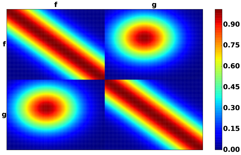
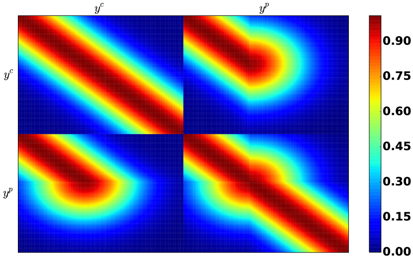
Figure 1: Illustration of the covariance matrix, $\Sigma$, for two functions $f$ and $g$ evaluated at points evenly distributed in [0,100] and crossing at $x_{p}=40$ (upper) and the resulting data covariance matrix, $\hat{\Sigma}$, for time course data $y^{c}$ and $y^{p}$ from a wild-type and perturbed system respectively (lower).

2.3 The data likelihood under the model

We define the perturbation time $x_{p}$ as the point where two time profiles first begin to diverge. If the time profiles are measured without noise then it would be trivial to identify this point. However, biological time course data from high-throughput experiments are often corrupted by significant biological and technical sources of noise and our task is to infer the perturbation time given noisy time course data. In order to do that we must first derive the likelihood function under the new model.

Let two sets of gene expression time course data, $y^{c}(\bf X)$ and $y^{p}(\bf X)$, represent noisy measurements with i.i.d Gaussian measurement noise, $\mathcal{N}(0,\sigma^{2}\mathbf{I})$, from the control condition and perturbed condition, respectively. A GP prior is placed on the mean functions underlying $y^{c}$ and $y^{p}$ and a time point $x_{p}$ is defined as the perturbation time point. The data model is defined as:

1. The two datasets $y^{c}$ and $y^{p}$ before $x_{p}$ are noise-corrupted versions of the same underlying mean function $f$ which has a GP prior,

   $$y^{c}(x_{n}) \sim \mathcal{N}(f(x_{n}),\sigma^{2}),$$

   $$y^{p}(x_{n}) \sim \mathcal{N}(f(x_{n}),\sigma^{2})\quad\mbox{for }x_{n}\leq x_{p}\ .$$

2. The mean function for $y^{c}$ stays intact after $x_{p}$ while the mean function for $y^{p}$ changes to follow $g$,

   $$y^{c}(x_{n}) \sim \mathcal{N}(f(x_{n}),\sigma^{2}),$$

   $$y^{p}(x_{n}) \sim \mathcal{N}(g(x_{n}),\sigma^{2})\quad\mbox{for }x_{n}>x_{p}\ ,$$

   where $f$ and $g$ are constrained to cross at $x_{p}$ and follow the GP described in Eqn. (2.2).

The joint distribution of $y^{c}$ and $y^{p}$ is then

$$p\left(y^{c}({\bf X}),y^{p}({\bf X})|x_{p}\right) =\exp\left(-\frac{1}{2}\begin{pmatrix}y^{c}\\ y^{p}\end{pmatrix}^{\top}\hat{\Sigma}^{-1}\begin{pmatrix}y^{c}\\ y^{p}\end{pmatrix}\right),$$ (7)

where the covariance matrix $\hat{\Sigma}$ can be worked out in terms of the covariance matrix $\Sigma$ for the joint distribution of $f$ and $g$ defined by Eqn. (6),

$$\hat{\Sigma}=\begin{pmatrix}\hat{K}_{y^{c}y^{c}}&\hat{K}_{y^{c}y^{p}}\\ \hat{K}_{y^{p}y^{c}}&\hat{K}_{y^{p}y^{p}}\end{pmatrix},$$ (8)

with

$$\scriptsize\hat{K}_{y^{c}({\bf X_{1}})y^{c}({\bf X_{2}})} =K_{f({\bf X}_{1})f({\bf X}_{2})}+\sigma^{2}\bf I\!\begin{array}[]{c}{\bf X}_{1}\in{\bf X},{\bf X}_{2}\in{\bf X}\end{array}$$

$$\hat{K}_{y^{c}({\bf X_{1}})y^{p}({\bf X_{2}})} =\left\{\begin{array}[]{c}K_{f({\bf X}_{1})f({\bf X}_{2})}\\ K_{f({\bf X}_{1})g({\bf X}_{2})}\end{array}\right.\!\begin{array}[]{l}{\bf X}_{1}\in{\bf X},{\bf X}_{2}\leq x_{p}\\ {\bf X}_{1}\in{\bf X},{\bf X}_{2}>x_{p}\end{array}$$

$$\hat{K}_{y^{p}({\bf X_{1}})y^{c}({\bf X_{2}})} =\left\{\begin{array}[]{c}K_{f({\bf X}_{1})f({\bf X}_{2})}\\ K_{g({\bf X}_{1})f({\bf X}_{2})}\end{array}\right.\!\begin{array}[]{l}{\bf X}_{1}\leq x_{p},{\bf X}_{2}\in{\bf X}\\ {\bf X}_{1}>x_{p},{\bf X}_{2}\in{\bf X}\end{array}$$

$$\hat{K}_{y^{p}({\bf X}_{1})y^{p}({\bf X}_{2})} =\left\{\begin{array}[]{c}K_{f({\bf X}_{1})f({\bf X}_{2})}+\sigma^{2}\bf I\\ K_{g({\bf X}_{1})f({\bf X}_{2})}\\ K_{f({\bf X}_{1})g({\bf X}_{2})}\\ K_{g({\bf X}_{1})g({\bf X}_{2})}+\sigma^{2}\bf I\end{array}\right.\!\begin{array}[]{l}{\bf X}_{1}\leq x_{p},{\bf X}_{2}\leq x_{p}\\ {\bf X}_{1}>x_{p},{\bf X}_{2}\leq x_{p}\\ {\bf X}_{2}>x_{p},{\bf X}_{1}\leq x_{p}\\ {\bf X}_{1}>x_{p},{\bf X}_{2}>x_{p}\end{array}$$

The lower panel in Fig. 1 shows the data covariance matrix $\hat{\Sigma}$ for $\bf X$ evenly spread in the range $[0,100]$ and with a perturbation occurring at $x_{p}=40$.

2.4 Posterior distribution of the perturbation point

According to Bayes’ rule the posterior distribution of $x_{p}$ is,

$$p(x_{p}|y^{c}({\bf X}),y^{p}({\bf X})) =\frac{p({y^{c}({\bf X}),y^{p}({\bf X})}|x_{p})p(x_{p})}{\int p({y^{c}({\bf X}),y^{p}({\bf X})}|x_{p})p(x_{p})dx_{p}}.$$

We assume a uniform prior on $x_{p}$ within the range $[x_{\mathrm{min}},x_{\mathrm{max}}]$ of the observed data. We use a simple discretization $x_{p}\in[x_{\mathrm{min}},x_{\mathrm{min}}+\delta,x_{\mathrm{min}}+2\delta,\ldots,x_{\mathrm{max}}]$ in this range. Then the posterior can be approximated as a simple summation over this grid,

$$p(x_{p}|y^{c}({\bf X}),y^{p}({\bf X}))\simeq\frac{p(y^{c}({\bf X}),y^{p}({\bf X})|x_{p})}{\sum_{x=x_{\mathrm{min}}}^{x=x_{\mathrm{max}}}p(y^{c}({\bf X}),y^{p}({\bf X})|x)},$$

only requiring that we evaluate the likelihood at each grid point. There are hyper-parameters $\theta$ also involved in the posterior distribution of $x_{p}$ which would potentially complicate matters. We choose to estimate these hyper-parameters prior to inferring $x_{p}$. To do this we use maximum likelihood optimisation for the case where $x_{p}$ approaches -$\infty$ which corresponds to the two GPs for the control and perturbed conditions being independent,

$$\hat{\theta}=\arg\!\max_{\theta}\left(\lim_{x_{p}\to-\infty}p_{\theta}(y^{c}({\bf X}),y^{p}({\bf X})|x_{p},\theta)\right)\ .$$

Since we have a simple histogram representation for the posterior distribution of the perturbation time point $x_{p}$ then we can easily estimate the mean, median or mode (MAP) of the posterior distribution to provide a point estimate.

2.5 Pre-filtering to remove non-DE genes

In many applications a large number of genes will show no strong evidence for DE at any time or will have a low signal-to-noise due to being weakly expressed. We therefore filter genes prior to using our model. A DE gene will be better represented by two independent GPs rather than a shared GP under control and perturbed conditions. We therefore filter genes using the log-likelihood ratio $r$ between the independent GP model (equivalent to $x_{p}$ approaching $-\infty$ in the perturbation model) and the integrated GP (with $x_{p}$ approaching $+\infty$):

$$r =\log\mathcal{L}(y_{c}({\bf X}),y_{p}({\bf X})|x_{p}\to-\infty)$$

$$-\log\mathcal{L}(y_{c}({\bf X}),y_{p}({\bf X})|x_{p}\to+\infty)$$ (9)

We note that it is difficult to distinguish genes with a late perturbation time from those that are non-DE and our filtering approach may remove some genuine late perturbation genes. In many applications we are primarily interested on relatively early perturbations (e.g. in the application considered here) in which case this will not significantly impact the results. In the Supplementary Section S4.2 we consider an alternative filtering approach which is based on detecting genes with time-varying profile in either the control or perturbed condition and is therefore less likely to filter out late $x_{p}$ genes.

The method has been implemented in the DEtime R-package (github.com/ManchesterBioinference/DEtime) and also as the DEtime kernel in the GPy Python package (github.com/SheffieldML/GPy). The running time for the whole genome (32578 genes) for the example in Section 3.3 on a Intel(R) Core(TM) i7-3770 CPU of 3.40GHz is around 11 hrs using the DEtime R-package.

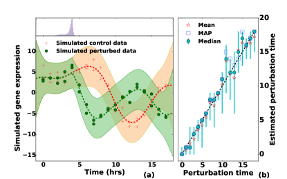
Figure 2: (a) The shaded area in the lower panel represents the 95% credible region of the GP regression result. In the top panel we show the inferred posterior distribution for the perturbation time $x_{p}$. (b) The mean, mode and median of the posterior distribution of $x_{p}$ with the 5-95 percentile coverage of the posterior distribution for 19 simulated dataset at different perturbation time points (dashed line shows the ground truth).

3 Results and Discussion

3.1 Generating simulated data

We generated data under a range of different scenarios to explore performance and robustness to deviations from the model. We generated expression profiles from three different covariance models, one matching the one used for inference and the other two generating rougher profiles. We then add noise using three different noise models, one matching the Gaussian model used for inference and two from heavier-tailed distributions.

1. profile₁: simulated noise-free profile generated from the model $\mathcal{GP}_{\theta}(\mathbf{0},\hat{\Sigma}_{\theta})$ with $\hat{\Sigma}_{\theta}$ given in Eqn. (8) assuming a squared exponential covariance function (recall Eqn. (1)) with the hyperparameters $\theta=\{\alpha=30.0,l=8.0\}$.

2. profile₂: simulated noise-free profile generated from above model with the covariance function in the form of a matern32 covariance function (Williams and Rasmussen, 2006) with the same hyperparameters as above.

3. profile₃: simulated noise-free profile generated from above model with the covariance function in the form of a matern12 covariance function (an Ornstein-Uhlenbeck (OU) process) with the same hyperparameters as above.

Nine simulated dataset are induced with different kinds of i.i.d noise on top of profile₁, profile₂ and profile₃, respectively: Gaussian $\mathcal{N}(1.5)$, Student-t distributed with 3 $(T(3))$ and 6 $(T(6))$ degrees of freedom. The simulated data are sampled every hour from 0 hrs until 18 hrs. We simulate data with a range of perturbation times ${\mathbf{x}_{p}}\in\{0,1,\cdots,17,18\}$ and 100 different sets of data are produced for each $x_{p}$ value.

Fig. 2 (a) shows an example of simulated data (using the profile₁$+\mathcal{N}(1.5)$ scenario) with two replicates and a perturbation at 4 hrs. The estimated posterior distribution of $x_{p}$ is shown in the upper panel and in the lower panel we show the GP regression function after fixing $x_{p}$ at the MAP value. In this case the MAP estimate for $x_{p}$ is very close to the ground truth. The mean, mode and median of the posterior distribution of $x_{p}$ for 19 simulated datasets are illustrated in Fig. 2 (b) together with the 5-95 percentile coverage of the posterior distribution. It is clear that the posterior distributions of the perturbation time cover the actual perturbation time to a great extent and that the three different point estimates are typically close to the ground truth values.

3.2 Comparison with a thresholding approach

Related methods have been introduced to identify regions of differential expression from time course data (Stegle et al., 2010; Heinonen et al., 2014). Such methods can in principle also be used to identify the perturbation time by locating the first time point where the DE score passes some threshold value. Here we compare our approach to the most recently published package of this type, developed by Heinonen et al. (2014) implemented in the nsgp R-package. The nsgp package infers the differentially expressed time periods and uses four likelihood ratios: marginal log-likelihood ratio (MLL), expected marginal log-likelihood ratio (EMLL), the posterior concentration (PC) and the noisy posterior concentration (NPC) to quantify these regions. We adopt thresholds of 0.5 and 1.0 to define the initial perturbation points, respectively. The mean, median and mode of the posterior distribution of the inferred perturbation points from our method are also computed. The performance of ranking $x_{p}$ using each method is measured by Spearman’s rank correlation coefficient with the known ground truth and the mean and standard deviation of the rank correlation coefficients across 100 dataset are illustrated in Table 1.

Table 1: Comparison of the means and stds of the Spearman’s rank correlation coefficients of the mean, median and MAP estimation of the perturbation times from our DEtime package and different likelihood ratios with various thresholds from the nsgp package. $M_{n}$ represents the $M$ ratio with a threshold of $n$.

R Package	DEtime			nsgp
Data	Mean	Median	MAP	MLL0.5	EMLL0.5	PC0.5	NPC0.5	MLL1.0	EMLL1.0	PC1.0	NPC1.0
profile1$+\mathcal{N}(1.5)$	0.94$\pm$0.04	0.94$\pm$0.04	0.93$\pm$0.05	-0.02$\pm$0.23	0.26$\pm$0.22	0.36$\pm$0.22	0.26$\pm$0.23	-0.02$\pm$0.23	0.67$\pm$0.16	0.29$\pm$0.22	0.48$\pm$0.21
profile2$+\mathcal{N}(1.5)$	0.90$\pm$0.06	0.90$\pm$0.06	0.88$\pm$0.08	-0.05$\pm$0.23	0.17$\pm$0.23	0.21$\pm$0.25	0.24$\pm$0.22	-0.06$\pm$0.23	0.57$\pm$0.20	0.18$\pm$0.24	0.42$\pm$0.21
profile3$+\mathcal{N}(1.5)$	0.93$\pm$0.04	0.93$\pm$0.04	0.92$\pm$0.05	-0.04$\pm$0.26	0.31$\pm$0.22	0.21$\pm$0.25	0.28$\pm$0.25	-0.05$\pm$0.26	0.75$\pm$0.16	0.20$\pm$0.23	0.47$\pm$0.23
profile1$+T(6)$	0.93$\pm$0.05	0.92$\pm$0.06	0.91$\pm$0.07	0.01$\pm$0.24	0.22$\pm$0.24	0.24$\pm$0.27	0.23$\pm$0.24	0.02$\pm$0.23	0.59$\pm$0.18	0.17$\pm$0.23	0.40$\pm$0.23
profile2$+T(6)$	0.87$\pm$0.07	0.86$\pm$0.07	0.83$\pm$0.09	0.04$\pm$0.23	0.27$\pm$0.25	0.08$\pm$0.24	0.15$\pm$0.22	0.03$\pm$0.23	0.42$\pm$0.24	0.02$\pm$0.24	0.28$\pm$0.24
profile3$+T(6)$	0.89$\pm$0.06	0.89$\pm$0.06	0.87$\pm$0.08	0.01$\pm$0.26	0.24$\pm$0.24	0.13$\pm$0.25	0.26$\pm$0.26	-0.00$\pm$0.27	0.64$\pm$0.20	0.07$\pm$0.25	0.41$\pm$0.23
profile1$+T(3)$	0.91$\pm$0.05	0.90$\pm$0.06	0.89$\pm$0.06	-0.02$\pm$0.24	0.14$\pm$0.22	0.19$\pm$0.22	0.20$\pm$0.21	-0.03$\pm$0.24	0.48$\pm$0.21	0.15$\pm$0.23	0.32$\pm$0.21
profile2$+T(3)$	0.83$\pm$0.09	0.83$\pm$0.10	0.80$\pm$0.11	-0.03$\pm$0.26	0.08$\pm$0.23	0.12$\pm$0.23	0.16$\pm$0.21	-0.04$\pm$0.26	0.36$\pm$0.23	0.05$\pm$0.22	0.24$\pm$0.24
profile3$+T(3)$	0.87$\pm$0.07	0.87$\pm$0.07	0.84$\pm$0.09	-0.01$\pm$0.25	0.20$\pm$0.21	0.09$\pm$0.23	0.20$\pm$0.18	0.00$\pm$0.25	0.54$\pm$0.22	0.09$\pm$0.23	0.33$\pm$0.23

From the table, it is clear that the mean, median and MAP estimates from the DEtime package provide better ranking performance. The results from the nsgp package vary significantly through different ratios and thresholds, among which, EMLL with threshold 1.0 performs the best in this task, giving rank correlation coefficient of 0.67$\pm$0.16 when tested on the simulated profile₁ contaminated with Gaussian noise $\mathcal{N}(0,1.5)$, which is still considerably lower than the rank correlation coefficients from mean, median or mode of the DEtime package. In order to compare the performance of the algorithm on data with varied signal-to-noise ratios, we adjusted the signal amplitude hyperparameter $\alpha$ and compared the results from DEtime and nsgp with $\alpha=1.5,10.0,20.0,30.0$. Supplementary Table S1 illustrates the results which shows the robustness of the proposed model. Supplementary Fig. S1 shows the errorbar of the mean, median, mode from DEtime package and EMLL with thresholds of 0.5 and 1.0 from nsgp package across 100 replicates along all perturbation times for all simulated datasets. We observe that the DEtime package provides reasonable estimation of the initial perturbation time under various noise distributions whereas the performance of the EMLL ratio from nsgp package varies substantially and its performance seems to be deteriorating with later initial perturbations.

We note that methods in the nsgp package are not designed specifically for the task of inferring the initial perturbation point as they were proposed for the more general problem of identifying DE regions. Nevertheless, a common application of time-series DE studies is to distinguish early and late DE events. We have demonstrated that one can obtain greater accuracy by focusing on this specific task rather than adapting a more general DE method.

3.3 Bacterial infection response in Arabidopsis thaliana

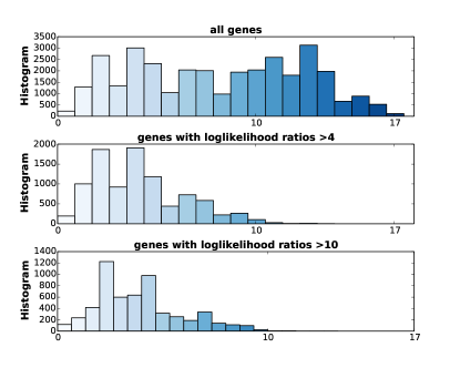
Figure S2: Histograms of estimated perturbation times for all the genes (upper panel), genes with loglikelihood ratios over 4 (middle) and genes with loglikelihood ratios over 10 (lower panel), respectively.

To determine the biological utility of estimating perturbation times, we re-examined a large dataset recently published by Lewis et al. (2015) that captures the transcriptional reprogramming associated with defence and disease development in Arabidopsis thaliana leaves inoculated with Pseudomonas syringae pv. tomato DC3000 and the non-pathogenic DC3000hrpA mutant strain. The differences in gene expression between these two challenges is a result of the action of virulence factors delivered by the DC3000 strain into the plant cell, in this case predominately the collaborative activities of 28 bacterial effector proteins. Figure 3 shows examples of an early and late perturbed gene identified by our method. A preliminary investigation of the perturbation times of differentially expressed genes revealed two peak times (Supplementary Figure S2), allowing genes to be assigned to one of three groups: early, intermediate and late perturbed genes. This initial characterisation was consistent with major phase changes in the infection process, and the onset of effector mediated transcriptional reprogramming: effectors are not delivered into plant cells until 90-120 minutes post inoculation (Grant et al., 2000), and do not promote bacterial growth until $\sim 8$ hpi, when they have effectively disabled host defence processes. This general progression is reflected in GO and pathway analysis outlined in Supplementary Section S4.1 and S4.2.

The recent study by Lewis et al. (2015) provided a comprehensive overview of the transition from defence to disease. Thus we investigated if the calculation of perturbation times provided supporting evidence and additional novel insights not highlighted by Lewis et al. (2015). To do so, genes were first grouped according to their GO or AraCyc Pathway annotation, and the cumulative perturbation time for each term calculated. The time at which more than $50\%$ of the genes associated with a particular term were perturbed could then be used to rank terms, allowing a high resolution understanding of the infection process. Heat maps showing the cumulative density function (CDF) of perturbation times for each term are shown in Supplementary Figures S4-S15. For clarity, we chose to focus predominately on the earliest processes perturbed by bacterial effectors as these are predicted to be processes integral to the suppression of innate immunity. As an initial proof of concept we focussed on the perturbation of hormone pathways, as modulation of these pathways are well known to be integral to pathogen virulence strategies (Fig. 4).

First we looked at abscisic acid (ABA) pathways, as it has previously been shown that DC3000 rapidly induces de novo ABA biosynthesis and hijacks ABA signalling pathways to promote virulence (de Torres-Zabala et al., 2007; de Torres Zabala et al., 2009). Fig. 4 shows a strong link between various GOs associated with ABA processes and early perturbation, which is what is predicted in the literature and demonstrated by Lewis et al. (2015). Amongst these early ABA signalling components induced were the classic ABA responsive TFs, RD26 and both ATAIB and AFP2 were induced around $2$ hpi. This prediction suggests that effectors are targeting ABA signaling very early in the infection process. Furthermore $>50\%$ of genes annotated with ‘regulation of abscisic acid biosynthetic process’ were perturbed by 2.3 hpi, consistent with measurable increased in de novo ABA biosynthesis 6 hpi (de Torres-Zabala et al., 2007), with subsequent perturbation of ‘cellular response to abscisic acid stimulus’ occurring by 3.5 hpi. Two genes showing perturbation at 4.1 hpi and annotated as ABA responsive, BLHL1 and TCP14, are predicted to be targeted by the DC3000 effector AvrPto in yeast two hybrid protein-protein interaction studies (Mukhtar et al., 2011). Moreover a knockout of TCP14 results in enhanced disease resistance to DC3000, consistent with TCP14 being a virulence target of effectors (Weßling et al., 2014). Subsequently, a number of ABA related pathways appear to be further targeted later in the infection. Interestingly ‘negative regulation of abscisic acid-activated signaling pathway’ was perturbed at 4.4 hpi suggesting this is an example of a failed host response (Lewis et al., 2015). Other notable perturbed ABA related ontologies included ‘abscisic acid transport’ (4.9 hpi), ‘abscisic acid catabolic process’ (5.1 hpi), ‘abscisic acid binding’ (5.1 hpi), ‘abscisic acid-activated signaling pathway’ (6.3 hpi), ‘abscisic acid biosynthetic process’ (7.2 hpi) and ‘positive regulation of abscisic acid-activated signaling pathway’ (7.2 hpi). Thus we can validate the importance of ABA in the infection process but, moreover, using our estimation of perturbation process we can see fine resolution of the increased impact of ABA biosynthesis and signaling on the infection process not evidenced by the previous analyses (Lewis et al., 2015) as illustrated in Fig. 4A.

As expected, we also identified strong early perturbations in salicylic acid (SA, Fig. 4B) related ontologies, as these are key targets for effector mediated suppression (DebRoy et al., 2004). For further validation, we looked at ontologies associated with the hormone jasmonic acid (JA, Fig. 4C). The JA ontologies show more delayed perturbation than ABA, particularly notably the ontologies associated with ‘response to jasmonic acid’ (2.3 hpi), ‘jasmonic biosynthetic processes’ (3.7 hpi) and ‘regulation of jasmonic acid mediate signaling pathways’ (3.8 hpi). This is consistent with the recent study by de Torres et al. (2015) using a specific targeted analysis of the same dataset which demonstrated that the JA contribution to DC3000 pathogenesis was preceded by a stronger ABA component. Thus both the ABA and JA analyses provide two examples that validate the utility of the perturbation estimation approach. Two other hormone signalling pathways, gibberellic acid (GA, Fig. 4D) and ethylene (ET, Fig. 4E), are predicted to play a minor role in establishment of virulence, with their contributions only occurring late in the infection process.

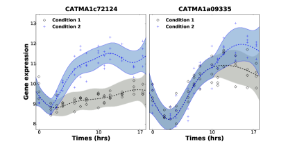
Figure 3: Examples of fitting the DEtime model to an early-perturbed (left) and late-perturbed gene from an experiment comparing arabadopsis leaves collected from plants infected with DC3000 (condition 1) and the mutant DC3000hrpA (condition 2). The shaded area represents the 95% credible region of the GP and the dashed line is the estimated mean of the model.

We next identified two signalling and two primary metabolism pathways that are predicted to be important in the early conflict between plant defence and pathogen virulence: MAP kinase kinase (MAPKK) activity, regulation of protein kinase activity, NAD biosynthesis process and methionine biosynthesis (Figure 4F/G).

MAMP signaling activates an early kinase phosphorylation cascade that initiates transcriptional activation (Zipfel, 2014), however little is known about the transcriptional activation or kinases. Remarkably, 8 out of the 10 MAPKKs encoded by the Arabidopsis genome were perturbed early. Given that these MAPKKs are responsible for phosphophorylation of the 20 downstream MAPKs their respective roles are naturally extensive. However, MAPKKs are strongly implicated in biotic stress. Most notably, the DC3000 effector HopF2 can interact with Arabidopsis MKK5 and most likely other MAPKKs to inhibit MAPKs and PAMP-triggered immunity. This is probably through MAPKK inhibition via ADP-ribosylation as HopF2 delivery inhibited PAMP-induced MPK phosphorylation (Wang et al., 2010). Functional evidence for a positive role of MKKs in defence comes from work in tobacco, where transient expression of AtMKK7/AtMKK9 and AtMKK4/AtMKK5 caused a hypersensitive response (Zhang et al., 2008). However, the roles of MKKs are likely to be multifunctional and may be manipulated by effectors to promote virulence. The MAPKK, MKK1 was shown to negatively regulate immunity (Kong et al., 2012). This may be through a dual role in activating ABA signalling as AtMKK1 as well as AtMKK2 and AtMKK3, could activate the ABA responsive RD29A promoter and MKK8 could activate the RD29B promoter (HUA et al., 2006). Concomitant with perturbation of the MKK pathway was a significant early perturbation of a sets of genes associated with regulation of protein kinase activity. Strikingly, these genes belong to a class of evolutionarily conserved kinases functioning as metabolic sensors and are activated in response to declining energy levels. Their co-regulation is probably because they typically function as a heterotrimeric complex comprising two regulatory subunits, $\beta$ and $\gamma$, and an $\alpha$-catalytic subunit. Intriguingly, a recent study predicted that the two clade A type 2C protein phosphatases that are negative regulators of ABA signalling, ABI1 and PP2CA, negatively regulate the Snf1-related protein kinase1 and that PP2C inhibition by ABA results in SnRK1 activation (Rodrigues et al., 2013). Moreover, SnRK1 and ABA were shown to induce largely overlapping transcriptional responses, thus these data reveal a previously unknown link between ABA and energy signalling during DC3000 infection.

A pathway intimately linked to energy signalling and redox reactions is NAD biosynthesis, one of the most significantly perturbed pathways following effector delivery (Figure 4G). Although powdery mildew infection of barley leaves was reported to be associated with increased NAD content more than 40 years ago (Ryrie and Scott, 1969) and recently the identification of the fin4 (flagellin insensitive 4) mutant as aspartate oxidase (Macho et al., 2012), a precursor of the NANP biosynthetic pathway, the role of pyridines in plant defence has received little attention. NAD and NADP play crucial roles in pro-oxidant and antioxidant metabolism and have been linked to biotic stress responses, including production of nitric oxide and metabolism of reactive lipid derivatives (Crawford and Guo, 2005; Mano et al., 2005). We highlight two possible, and contrasting, roles for rapid induction of NAD biosynthesis components by effectors. First, it has recently been shown that chloroplast ROS production is influenced by NADP:NADPH ratios and bacteria effector delivery rapidly suppresses a MAMP triggered chloroplast burst of hydrogen peroxide in an ABA dependent manner (de Torres Zabala et al., 2015). Secondly, poly(ADP-Ribose) polymerases (PARPs) is emerging as a key regulator of defence responses. PARPs are important NAD+ consuming enzymes induced by biotic stress, polymerising long poly(ADP-ribose) chains on target proteins including histones. (Adams-Phillips et al., 2010) reported a $40\%$ to $50\%$ decrease in NAD+ 12 hpi of DC3000 challenged leaves compared to a mock control and $\sim 50\%$ increase in total cellular and nuclear poly(ADP-Rib) polymers (Adams-Phillips et al., 2010). Consistent with these results, a knockout of PARP2, which is induced by MAMPs, restricts DC3000 growth (Song et al., 2015) demonstrating that loss of poly(ADP-ribosyl)ation activity affects the capacity of Arabidopsis to limit DC3000 growth.

The second primary metabolism example we choose to highlight is the very rapid induction methionine biosynthesis pathway (Figure 4G). Methionine is a sulphur amino acid involved in multiple cellular processes from being a protein constituent, to initiation of mRNA translation as well as functioning as a regulatory molecule in the form of S-adenosylmethionine (SAM). There are 13 unique genes associated with this ontology, and while it is outside the scope of this manuscript to explore these in detail it is worth noting that this includes DMR1 (Downy Mildew Resistance 1) (van Damme et al., 2009), encoding homoserine kinase, which produces O-phospho-L-homoserine, a compound at the branching point of methionine and threonine biosynthesis. Mutations in dmr1 lead to elevated foliar homoserine and resistance to the biotrophic pathogens Hyaloperonospora arabidopsidis, Oidium neolycopersici, F. culmorum and F. graminearum, although the mechanism has yet to be identified (van Damme et al., 2009; Huibers et al., 2013; Brewer et al., 2014).

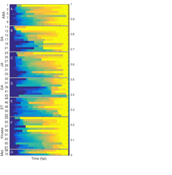
Figure 4: The cumulative distribution of inferred perturbation times of gene sets associated with hormone, signalling and metabolism related gene ontology terms. See Supplementary Table LABEL:Tab:11 for key.

Thus in summary, we have validated perturbation times against previous analyses, and provide four new examples derived from examining early perturbation times of biological pathways to identify novel signalling and, particularly, primary metabolic pathways that are implicated in the transition from defence to disease following infection with DC3000. These examples provide compelling leads for further investigation.

4 Conclusion

We have introduced a fully Bayesian approach to infer the initial point where two gene expression time profiles diverge using a novel GP regression approach. We model the data as noise-corrupted samples coming from a shared function prior to some “perturbation time” after which it splits into two conditionally independent functions. The full posterior distribution of the perturbation point is obtained through a simple histogram approach, providing a straightforward method to infer the divergence time between two gene expression time profiles under different conditions. The proposed method is applied to a study of the timing of transcriptional changes in Arabidopsis thaliana under a bacterial challenge with a wild-type and disarmed strain. Analysis of differences in the gene expression profiles between strains is shown to be informative about the immune response.

Many transcriptional perturbation experiments are focused on a single perturbation. However, multiple perturbations occurring at different times or a single perturbation targeting many conditions will be needed to unmask complex gene regulatory strategies. An interesting future line of research would be the development of GP covariance structures to uncover the ordering of events under these more general scenarios.

Supplementary Files

S1 Model Derivation

Consider the case where two time profiles, $f({{\bf X}})$ and $g({{\bf Z}})$, evaluated at specified sets of time points ${\bf X}$ and ${\bf Z}$, respectively, cross at the point $x_{p}$ with $f(x_{p})=g(x_{p})=u$ at the crossing point. We use the same Gaussian process (GP) prior for each function,

$$f({{\bf X}}) \sim\mathcal{GP}(\mu(x),K(x,x^{\prime})),$$

$$g({{\bf Z}}) \sim\mathcal{GP}(\mu(z),K(z,z^{\prime})).$$

Imposing the constraint that the functions cross at $x_{p}$, $p(f|{\bf X},u)$ and $p(g|{\bf Z},u)$ are then,

$$p(f({\bf X})|u) \sim\mathcal{N}(\mu_{\bf X},C_{\bf X}),$$

$$p(g({\bf Z})|u) \sim\mathcal{N}(\mu_{\bf Z},C_{\bf Z}),$$

with

$$\mu_{\bf X} = \frac{K({\bf X},x_{p})u}{K(x_{p},x_{p})},$$

$$C_{\bf X} = K({\bf X},{\bf X})-\frac{K({\bf X},x_{p})K({\bf X},x_{p})^{\top}}{K(x_{p},x_{p})},$$

$$\mu_{\bf Z} = \frac{K({\bf Z},x_{p})u}{K(x_{p},x_{p})},$$

$$C_{\bf Z} = K({\bf Z},{\bf Z})-\frac{K({\bf Z},x_{p})K({\bf Z},x_{p})^{\top}}{K(x_{p},x_{p})}.$$

In practice, the time profiles $f({\bf X})$ and $g({\bf Z})$ are typically measured at the same time points, so that ${\bf Z}$ can be replaced by ${\bf X}$. The joint probably distribution of f and g is then obtained by integrating over the latent function $u=f(x_{p})$ which has a Gaussian distribution with variance $k(x_{p},x_{p})=\alpha$, $u\sim{\cal N}(0,\alpha)$, so that:

$$p(f({\bf X}),g({\bf X}))\!\!\!\! = \!\!\!\!\int p(f|{{\bf X}},u)p(g|{\bf X},u)p(u)du,$$

$$\propto \int\exp\left[-\frac{1}{2}(f-\mu_{\bf X})C_{\bf X}^{-1}(f-\mu_{\bf X})^{T}-\frac{1}{2}(g-\mu_{\bf X})C_{\bf X}^{-1}(g-\mu_{\bf X})^{T}-\frac{u^{2}}{2\alpha}\right]du,$$

$$\propto \exp\left(-\frac{f^{T}C_{\bf X}^{-1}f+g^{T}C_{\bf X}^{-1}g}{2}\right)\int\exp\left[(f^{T}C_{\bf X}^{-1}k_{\bf X}+g^{T}C_{\bf X}^{-1}k_{\bf X})\frac{u}{\alpha}-k_{\bf X}^{T}C_{\bf X}^{-1}k_{\bf X}\frac{u^{2}}{\alpha^{2}}-\frac{u^{2}}{2\alpha}\right]du,$$

$$= \exp\left(-\frac{f^{T}C_{\bf X}^{-1}f+g^{T}C_{\bf X}^{-1}g}{2}\right)\int\exp\left\{-\frac{2k_{\bf X}^{T}C_{\bf X}^{-1}k_{\bf X}+\alpha}{2\alpha^{2}}\right.$$

$$\cdot\left.\left[\left(u-\frac{\alpha(f^{T}C_{\bf X}^{-1}k_{\bf X}+g^{T}C_{\bf X}^{-1}k_{\bf X})}{2k_{\bf X}^{T}C_{\bf X}^{-1}k_{\bf X}+\alpha}\right)^{2}-\left(\frac{\alpha(f^{T}C_{\bf X}^{-1}k_{\bf X}+g^{T}C_{\bf X}^{-1}k_{\bf X})}{2k_{\bf X}^{T}C_{\bf X}^{-1}k_{\bf X}+\alpha}\right)^{2}\right]\right\}du,$$

$$\propto \exp\left(-\frac{f^{T}C_{\bf X}^{-1}f+g^{T}C_{\bf X}^{-1}g}{2}+\frac{(f^{T}C_{\bf X}^{-1}k_{\bf X}+g^{T}C_{\bf X}^{-1}k_{\bf X})^{2}}{4k_{\bf X}^{T}C_{\bf X}^{-1}k_{\bf X}+2\alpha}\right),$$

$$= \exp\left[-\frac{1}{2}f^{T}\left(C_{\bf X}^{-1}-\frac{C_{\bf X}^{-1}k_{{\bf X}}k_{{\bf X}}^{T}C_{{\bf X}}^{-1}}{2k_{{\bf X}}^{T}C_{{\bf X}}^{-1}k_{{\bf X}}+\alpha}\right)f-\frac{1}{2}g^{T}\left(C_{\bf X}^{-1}-\frac{C_{{\bf X}}^{-1}k_{{\bf X}}k_{{\bf X}}^{T}C_{{\bf X}}^{-1}}{2k_{{\bf X}}^{T}C_{{\bf X}}^{-1}k_{{\bf X}}+\alpha}\right)g\right.$$

$$+\left.\frac{1}{2}g^{T}\left(\frac{C_{{\bf X}}^{-1}k_{{\bf X}}k_{{\bf X}}^{T}C_{{\bf X}}^{-1}}{2k_{{\bf X}}^{T}C_{{\bf X}}^{-1}k_{{\bf X}}+\alpha}\right)f+\frac{1}{2}f^{T}\left(\frac{C_{{\bf X}}^{-1}k_{{\bf X}}k_{{\bf X}}^{T}C_{{\bf X}}^{-1}}{2k_{{\bf X}}^{T}C_{{\bf X}}^{-1}k_{{\bf X}}+\alpha}\right)g\right],$$

$$= \exp\left(-\frac{1}{2}\begin{pmatrix}f\\ g\end{pmatrix}^{T}\begin{pmatrix}A&B\\ B&A\end{pmatrix}\begin{pmatrix}f\\ g\end{pmatrix}\right)=\exp\left(-\frac{1}{2}\begin{pmatrix}f\\ g\end{pmatrix}^{T}\begin{pmatrix}K_{ff}&K_{fg}\\ K_{fg}^{T}&K_{gg}\end{pmatrix}^{-1}\begin{pmatrix}f\\ g\end{pmatrix}\right),$$

where $K$ and $k_{\bf X}$ are abbreviations for $K(\bf X,X)$ and $K({\bf X},x_{p})$, respectively, and

$$A = C_{{\bf X}}^{-1}-\frac{C_{{\bf X}}^{-1}k_{{\bf X}}k_{{\bf X}}^{T}C_{{\bf X}}^{-1}}{\alpha+2k_{{\bf X}}^{T}C_{{\bf X}}^{-1}k_{{\bf X}}},$$

$$B = -\frac{C_{{\bf X}}^{-1}k_{{\bf X}}k_{{\bf X}}^{T}C_{{\bf X}}^{-1}}{\alpha+2k_{{\bf X}}^{T}C_{{\bf X}}^{-1}k_{{\bf X}}}.$$

Let us say $p_{1}=k_{{\bf X}}^{T}K^{-1}k_{{\bf X}}$ and $p_{2}=k_{{\bf X}}^{T}C^{-1}k_{{\bf X}}$,

$$p_{2}=k_{{\bf X}}^{T}C_{{\bf X}}^{-1}k_{{\bf X}} = \frac{\alpha k_{{\bf X}}^{T}K^{-1}k_{{\bf X}}}{\alpha-k_{{\bf X}}^{T}K^{-1}k_{{\bf X}}}=\frac{\alpha p_{1}}{\alpha-p_{1}},$$

$$B = -\frac{C_{{\bf X}}^{-1}k_{{\bf X}}k_{{\bf X}}^{T}C_{{\bf X}}^{-1}}{\alpha+2k_{{\bf X}}^{T}C_{{\bf X}}^{-1}k_{{\bf X}}}=-\frac{\alpha^{2}K^{-1}k_{{\bf X}}k_{{\bf X}}^{T}K^{-1}}{(\alpha-p_{1})^{2}(\alpha+2p_{2})}=-\frac{\alpha K^{-1}k_{{\bf X}}k_{{\bf X}}^{T}K^{-1}}{(\alpha^{2}-p_{1}^{2})},$$

$$A = C_{{\bf X}}^{-1}-B=K^{-1}+\frac{K^{-1}k_{{\bf X}}k_{{\bf X}}^{T}K^{-1}}{\alpha-p_{1}}-\frac{\alpha K^{-1}k_{{\bf X}}k_{{\bf X}}^{T}K^{-1}}{(\alpha^{2}-p_{1}^{2})}=K^{-1}+\frac{p_{1}K^{-1}k_{{\bf X}}k_{{\bf X}}^{T}K^{-1}}{(\alpha^{2}-p_{1}^{2})},$$

so,

$$A^{-1} = K-\frac{\frac{p_{1}KK^{-1}k_{{\bf X}}k_{{\bf X}}^{T}K^{-1}K}{(\alpha^{2}-p_{1}^{2})}}{1+\frac{p_{1}k_{{\bf X}}^{T}K^{-1}KK^{-1}k_{{\bf X}}}{(\alpha^{2}-p_{1}^{2})}}=K-\frac{p_{1}k_{bX}k_{{\bf X}}^{T}}{(\alpha^{2}-p_{1}^{2})+p_{1}k_{{\bf X}}^{T}K^{-1}k_{{\bf X}}}=K-\frac{p_{1}}{\alpha^{2}}k_{{\bf X}}k_{{\bf X}}^{T},$$

then,

$$K_{ff} = (A-BA^{-1}B)^{-1}=K,$$

$$K_{fg} = -(A-BA^{-1}B)^{-1}BA^{-1}=K\frac{\alpha K^{-1}k_{{\bf X}}k_{{\bf X}}^{T}K^{-1}}{(\alpha^{2}-p_{1}^{2})}\{K-\frac{p_{1}}{\alpha^{2}}k_{{\bf X}}k_{{\bf X}}^{T}\}=\frac{k_{{\bf X}}k_{{\bf X}}^{T}}{\alpha},$$

$$K_{gf} = -A^{-1}B(A-BA^{-1}B)^{-1}=\frac{k_{{\bf X}}k_{{\bf X}}^{T}}{\alpha},$$

$$K_{gg} = (A-BA^{-1}B)^{-1}=K.$$

S2 Covariance matrix of the perturbation model

Without loss of generality, we consider the discrete functions $\{f(x_{i}):i=1:n\}$ and $\{g(x_{j}):j=1:n\}$, here $n$ is the length of the data. Assuming that the perturbation occurs at $x=x_{p}$, according to the perturbation model assumption, the data $\{f(x_{i}):i=1:n\}$ and $\{g(x_{j}):j=1:p\}$ can be represented by the same GP while $\{g(x_{j}):j=p+1:n\}$ are perturbed and represented by another GP, therefore, the matrix blocks $K_{ff}$, $K_{fg}$, $K_{gf}$ and $K_{gg}$ will be changed accordingly to $\bar{K}_{ff}$, $\bar{K}_{fg}$, $\bar{K}_{gf}$ and $\bar{K}_{gg}$,

$$\bar{K}_{ff}^{[1:n,1:n]} = K_{ff}^{[1:n,1:n]},$$

$$\bar{K}_{fg}^{[1:n,1:p]} = K_{ff}^{[1:n,1:p]},$$

$$\bar{K}_{fg}^{[1:n,p+1:n]} = K_{fg}^{[1:n,p+1:n]},$$

$$\bar{K}_{gg}^{[1:p,1:p]} = K_{ff}^{[1:p,1:p]},$$

$$\bar{K}_{gg}^{[1:p,p+1:n]} = K_{fg}^{[1:p,p+1:n]},$$

$$\bar{K}_{gg}^{[p+1:n,1:p]} = K_{gf}^{[p+1:n,1:p]},$$

$$\bar{K}_{gg}^{[p+1:n,p+1:n]} = K_{gg}^{[p+1:n,p+1:n]},$$

$$\bar{K}_{gf}^{[1:n,1:n]} = [\bar{K}_{fg}^{[1:n,1:n]}]^{T},$$

here $K_{m}^{[a,b]}$ represents the element at row $a$ and column $b$ of the matrix $K_{m}$. Taking into account the noisy measurements, a small noise variance $\sigma^{2}$ will be added to the diagonal of the covariance matrix, and eventually the covariance matrix for $f$ and $g$, $\bar{K}_{final}$, becomes

$$\bar{K}_{final} = \begin{pmatrix}\bar{K}_{ff}&\bar{K}_{fg}\\ \bar{K}_{gf}&\bar{K}_{gg}\end{pmatrix}+\sigma^{2}\mathit{I_{(2n\times 2n)}}.$$

When replicates are encountered in the model, the matrix will have to be repeated, so in the case of two replicates, the covariance matrix $\bar{K}_{final}$ becomes

$$\bar{K}_{final} = \begin{pmatrix}\bar{K}_{ff}&\bar{K}_{ff}&\bar{K}_{fg}&\bar{K}_{fg}\\ \bar{K}_{ff}&\bar{K}_{ff}&\bar{K}_{fg}&\bar{K}_{fg}\\ \bar{K}_{fg}&\bar{K}_{fg}&\bar{K}_{gg}&\bar{K}_{gg}\\ \bar{K}_{fg}&\bar{K}_{fg}&\bar{K}_{gg}&\bar{K}_{gg}\end{pmatrix}+\sigma^{2}\mathit{I_{(4n\times 4n)}}.$$

S3 Results on simulated data

We generated data under a range of different scenarios to explore performance and robustness to deviations from the model. We generated expression profiles from three different covariance models, one matching the one used for inference and other two generating rougher profiles. We then add noise using three different noise models, one matching the Gaussian model used for inference and two from heavier-tailed distributions with the same set of hyperparameters.

1. profile₁: simulated data generated from the model $\mathcal{GP}_{\theta}(\mathbf{0},\hat{\Sigma}_{\theta})$ with $\hat{\Sigma}_{\theta}$ assuming a squared exponential covariance function.

2. profile₂: simulated data generated from above Gaussian process model with the covariance function in the form of a matern32 covariance function.

3. profile₃: simulated data generated from above Gaussian process model with the covariance function in the form of a matern12 covariance function.

Nine simulated dataset were induced with different kinds of i.i.d noise on top of profile₁, profile₂ and profile₃, respectively: Gaussian $\mathcal{N}(0,1.5)$, Student-t distributed with 3 $(T(3))$ and 6 $(T(6))$ degrees of freedom. The simulated data were sampled every hour from 0hrs till 18hrs. Perturbation times ${\mathbf{x}_{p}}$ were set in the range $\{0,1,\cdots,17,18\}$ and 100 different sets of data were produced for each $x_{p}$ with each dataset having 2 replicates.

Here we compare our approach to the most recently published package of this type, developed by Heinonen et al. (2014) implemented in the nsgp R-package. The nsgp package infers the differentially expressed time periods and uses four likelihood ratios: marginal log-likelihood ratio (MLL), expected marginal log-likelihood ratio (EMLL), the posterior concentration (PC) and the noisy posterior concentration (NPC) to quantify these regions. We adopt thresholds of 0.5 and 1.0 to define the initial perturbation points, respectively. The mean, median and mode of the posterior distribution of the inferred perturbation points from our method are also computed. In order to test the robustness of our proposed model, we fixed the lengthscale parameter ($l=8.0$) and varied the amplitude parameter ($\alpha=30.0,20.0,10.0,1.5$) in different kernel profiles. The performance of ranking $x_{p}$ using each method is measured by Spearman’s rank correlation coefficient with the known ground truth and the mean and standard deviation of the rank correlation coefficients across 100 dataset are illustrated in Table S1. It is clear that the proposed algorithm provides robust estimations to the perturbation points under reasonable noise conditions. EMLL with threshold of 1.0 provides the best results among those from nsgp package, however, its performance is much worse than those from the DEtime package. The mean, meadian and MAP results from DEtime package and EMLL_0.5 and EMLL_1.0 from nsgp package with $\alpha=30.0$ are illustrated in Fig. S1.

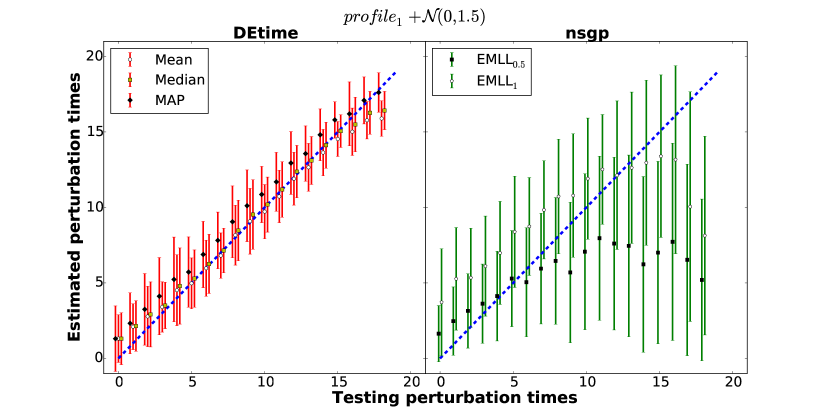
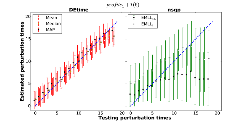
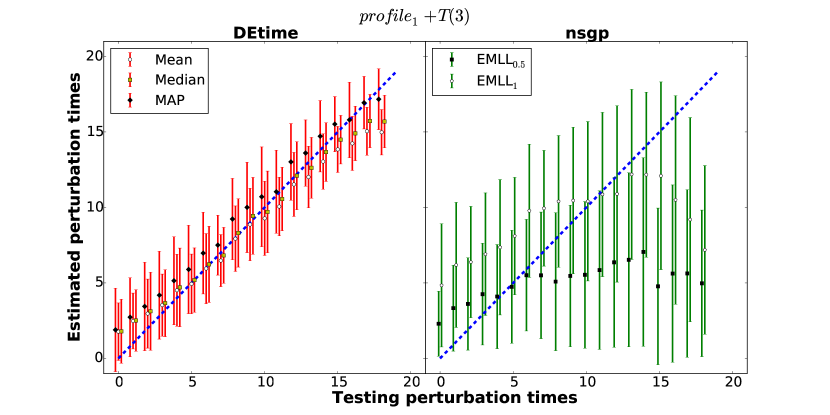
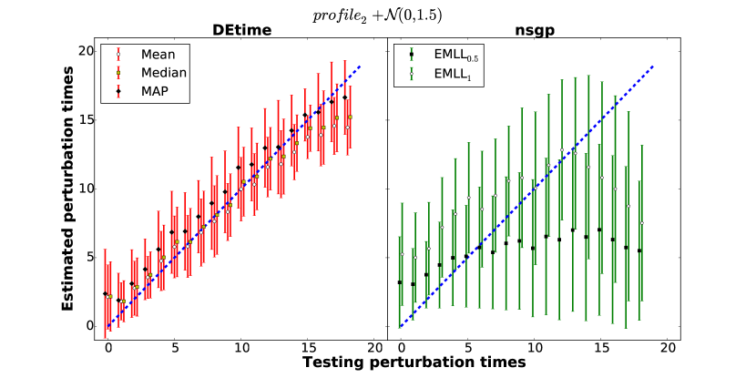
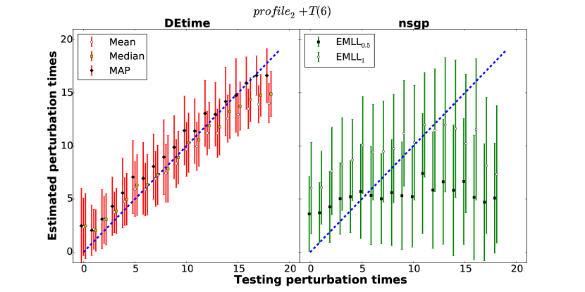
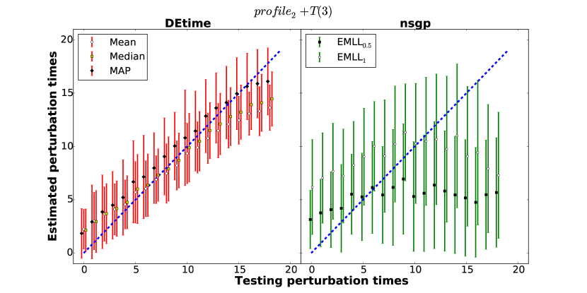
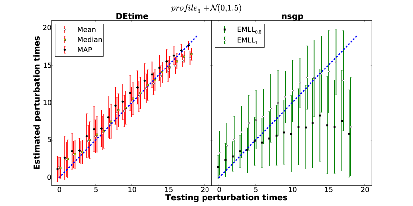
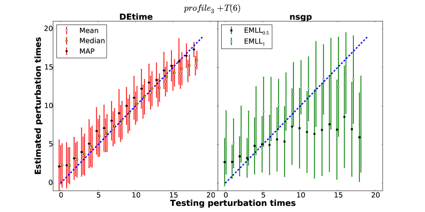
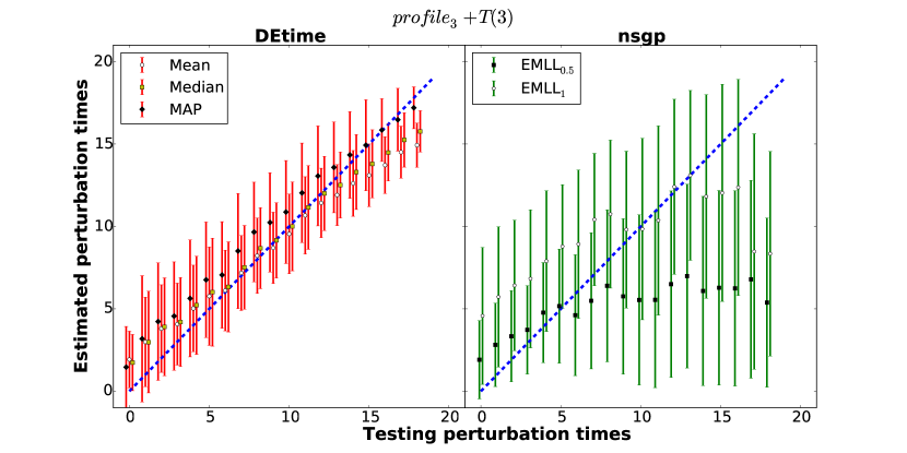
Figure S1: Estimated mean, median, MAP (from DEtime package), EMLL_0.5, EMLL_1.0 (from nsgp package) and 5-95 percentile coverage of the posterior distributions on tested perturbation times of 100 dataset each generated over the nine types of simulated data with hyperparameters $\alpha=30.0,l=8.0$.

Table S1: Comparison of the means and stds of the Spearman’s rank correlation coefficients of the mean, median and MAP estimation of the perturbation times from our DEtime package and different likelihood ratios with various thresholds from the nsgp package under various $\alpha$. $M_{n}$ represents the $M$ ratio with a threshold of $n$.

R Package	DEtime			nsgp
$\alpha=30.0$
Data	Mean	Median	MAP	MLL0.5	EMLL0.5	PC0.5	NPC0.5	MLL1.0	EMLL1.0	PC1.0	NPC1.0
profile1$+\mathcal{N}(1.5)$	0.94$\pm$0.04	0.94$\pm$0.04	0.93$\pm$0.05	-0.02$\pm$0.23	0.26$\pm$0.22	0.36$\pm$0.22	0.26$\pm$0.23	-0.02$\pm$0.23	0.67$\pm$0.16	0.29$\pm$0.22	0.48$\pm$0.21
profile2$+\mathcal{N}(1.5)$	0.90$\pm$0.06	0.90$\pm$0.06	0.88$\pm$0.08	-0.05$\pm$0.23	0.17$\pm$0.23	0.21$\pm$0.25	0.24$\pm$0.22	-0.06$\pm$0.23	0.57$\pm$0.20	0.18$\pm$0.24	0.42$\pm$0.21
profile3$+\mathcal{N}(1.5)$	0.93$\pm$0.04	0.93$\pm$0.04	0.92$\pm$0.05	-0.04$\pm$0.26	0.31$\pm$0.22	0.21$\pm$0.25	0.28$\pm$0.25	-0.05$\pm$0.26	0.75$\pm$0.16	0.20$\pm$0.23	0.47$\pm$0.23
profile1$+T(6)$	0.93$\pm$0.05	0.92$\pm$0.06	0.91$\pm$0.07	0.01$\pm$0.24	0.22$\pm$0.24	0.24$\pm$0.27	0.23$\pm$0.24	0.02$\pm$0.23	0.59$\pm$0.18	0.17$\pm$0.23	0.40$\pm$0.23
profile2$+T(6)$	0.87$\pm$0.07	0.86$\pm$0.07	0.83$\pm$0.09	0.04$\pm$0.23	0.27$\pm$0.25	0.08$\pm$0.24	0.15$\pm$0.22	0.03$\pm$0.23	0.42$\pm$0.24	0.02$\pm$0.24	0.28$\pm$0.24
profile3$+T(6)$	0.89$\pm$0.06	0.89$\pm$0.06	0.87$\pm$0.08	0.01$\pm$0.26	0.24$\pm$0.24	0.13$\pm$0.25	0.26$\pm$0.26	-0.00$\pm$0.27	0.64$\pm$0.20	0.07$\pm$0.25	0.41$\pm$0.23
profile1$+T(3)$	0.91$\pm$0.05	0.90$\pm$0.06	0.89$\pm$0.06	-0.02$\pm$0.24	0.14$\pm$0.22	0.19$\pm$0.22	0.20$\pm$0.21	-0.03$\pm$0.24	0.48$\pm$0.21	0.15$\pm$0.23	0.32$\pm$0.21
profile2$+T(3)$	0.83$\pm$0.09	0.83$\pm$0.10	0.80$\pm$0.11	-0.03$\pm$0.26	0.08$\pm$0.23	0.12$\pm$0.23	0.16$\pm$0.21	-0.04$\pm$0.26	0.36$\pm$0.23	0.05$\pm$0.22	0.24$\pm$0.24
profile3$+T(3)$	0.87$\pm$0.07	0.87$\pm$0.07	0.84$\pm$0.09	-0.01$\pm$0.25	0.20$\pm$0.21	0.09$\pm$0.23	0.20$\pm$0.18	0.00$\pm$0.25	0.54$\pm$0.22	0.09$\pm$0.23	0.33$\pm$0.23
$\alpha=20.0$
Data	Mean	Median	MAP	MLL0.5	EMLL0.5	PC0.5	NPC0.5	MLL1.0	EMLL1.0	PC1.0	NPC1.0
profile1$+\mathcal{N}(1.5)$	0.93$\pm$0.05	0.93$\pm$0.05	0.91$\pm$0.07	-0.02$\pm$0.23	0.20$\pm$0.22	0.29$\pm$0.20	0.22$\pm$0.18	0.01$\pm$0.23	0.62$\pm$0.18	0.26$\pm$0.23	0.47$\pm$0.20
profile2$+\mathcal{N}(1.5)$	0.88$\pm$0.08	0.88$\pm$0.10	0.86$\pm$0.10	0.01$\pm$0.23	0.16$\pm$0.23	0.17$\pm$0.23	0.25$\pm$0.24	-0.01$\pm$0.25	0.46$\pm$0.24	0.11$\pm$0.23	0.34$\pm$0.22
profile3$+\mathcal{N}(1.5)$	0.91$\pm$0.05	0.91$\pm$0.06	0.89$\pm$0.06	-0.05$\pm$0.25	0.34$\pm$0.20	0.18$\pm$0.24	0.31$\pm$0.22	-0.05$\pm$0.24	0.66$\pm$0.18	0.12$\pm$0.24	0.46$\pm$0.23
profile1$+T(6)$	0.89$\pm$0.07	0.89$\pm$0.08	0.86$\pm$0.09	-0.04$\pm$0.22	0.12$\pm$0.22	0.18$\pm$0.21	0.17$\pm$0.25	-0.03$\pm$0.22	0.43$\pm$0.20	0.12$\pm$0.21	0.34$\pm$0.21
profile2$+T(6)$	0.82$\pm$0.11	0.82$\pm$0.12	0.78$\pm$0.13	-0.04$\pm$0.25	0.08$\pm$0.20	0.07$\pm$0.23	0.14$\pm$0.21	-0.03$\pm$0.25	0.35$\pm$0.22	0.05$\pm$0.22	0.24$\pm$0.23
profile3$+T(6)$	0.87$\pm$0.06	0.87$\pm$0.07	0.84$\pm$0.08	-0.04$\pm$0.25	0.22$\pm$0.21	0.07$\pm$0.23	0.22$\pm$0.23	-0.04$\pm$0.25	0.51$\pm$0.21	0.09$\pm$0.21	0.35$\pm$0.22
profile1$+T(3)$	0.87$\pm$0.07	0.87$\pm$0.07	0.85$\pm$0.08	0.03$\pm$0.22	0.13$\pm$0.20	0.15$\pm$0.22	0.18$\pm$0.18	0.03$\pm$0.22	0.46$\pm$0.21	0.09$\pm$0.23	0.31$\pm$0.21
profile2$+T(3)$	0.77$\pm$0.10	0.76$\pm$0.11	0.71$\pm$0.15	-0.01$\pm$0.25	0.04$\pm$0.22	0.06$\pm$0.25	0.13$\pm$0.26	-0.01$\pm$0.25	0.31$\pm$0.24	0.07$\pm$0.21	0.21$\pm$0.25
profile3$+T(3)$	0.85$\pm$0.07	0.85$\pm$0.08	0.83$\pm$0.09	-0.02$\pm$0.25	0.12$\pm$0.21	0.05$\pm$0.24	0.16$\pm$0.21	-0.00$\pm$0.25	0.46$\pm$0.24	0.03$\pm$0.23	0.23$\pm$0.24
$\alpha=10.0$
Data	Mean	Median	MAP	MLL0.5	EMLL0.5	PC0.5	NPC0.5	MLL1.0	EMLL1.0	PC1.0	NPC1.0
profile1$+\mathcal{N}(1.5)$	0.89$\pm$0.06	0.88$\pm$0.07	0.85$\pm$0.10	-0.02$\pm$0.25	0.18$\pm$0.22	0.18$\pm$0.25	0.23$\pm$0.22	-0.03$\pm$0.24	0.45$\pm$0.24	0.13$\pm$0.23	0.34$\pm$0.23
profile2$+\mathcal{N}(1.5)$	0.81$\pm$0.11	0.80$\pm$0.12	0.76$\pm$0.13	-0.01$\pm$0.22	0.09$\pm$0.22	0.07$\pm$0.22	0.19$\pm$0.20	-0.01$\pm$0.23	0.34$\pm$0.24	0.04$\pm$0.22	0.23$\pm$0.21
profile3$+\mathcal{N}(1.5)$	0.88$\pm$0.06	0.88$\pm$0.06	0.85$\pm$0.09	-0.03$\pm$0.20	0.20$\pm$0.21	0.03$\pm$0.25	0.25$\pm$0.21	-0.03$\pm$0.21	0.55$\pm$0.19	0.03$\pm$0.23	0.32$\pm$0.21
profile1$+T(6)$	0.83$\pm$0.08	0.83$\pm$0.09	0.80$\pm$0.11	-0.03$\pm$0.25	0.16$\pm$0.24	0.11$\pm$0.25	0.20$\pm$0.24	-0.02$\pm$0.25	0.36$\pm$0.23	0.05$\pm$0.24	0.26$\pm$0.22
profile2$+T(6)$	0.75$\pm$0.12	0.73$\pm$0.12	0.69$\pm$0.14	-0.02$\pm$0.23	0.10$\pm$0.21	0.03$\pm$0.25	0.15$\pm$0.22	-0.01$\pm$0.24	0.27$\pm$0.21	-0.01$\pm$0.23	0.16$\pm$0.22
profile3$+T(6)$	0.82$\pm$0.10	0.82$\pm$0.11	0.77$\pm$0.14	-0.02$\pm$0.23	0.14$\pm$0.23	0.03$\pm$0.24	0.19$\pm$0.24	-0.01$\pm$0.23	0.37$\pm$0.20	0.03$\pm$0.23	0.23$\pm$0.22
profile1$+T(3)$	0.82$\pm$0.09	0.81$\pm$0.11	0.77$\pm$0.11	0.04$\pm$0.22	0.07$\pm$0.22	0.05$\pm$0.25	0.10$\pm$0.24	0.04$\pm$0.23	0.30$\pm$0.21	0.04$\pm$0.25	0.17$\pm$0.23
profile2$+T(3)$	0.74$\pm$0.12	0.73$\pm$0.12	0.69$\pm$0.14	-0.02$\pm$0.23	0.11$\pm$0.21	0.02$\pm$0.24	0.15$\pm$0.22	-0.02$\pm$0.24	0.27$\pm$0.21	-0.01$\pm$0.23	0.16$\pm$0.22
profile3$+T(3)$	0.75$\pm$0.12	0.75$\pm$0.13	0.70$\pm$0.15	0.01$\pm$0.22	0.08$\pm$0.24	-0.00$\pm$0.24	0.12$\pm$0.23	0.00$\pm$0.22	0.29$\pm$0.24	0.03$\pm$0.24	0.15$\pm$0.25
$\alpha=1.5$
Data	Mean	Median	MAP	MLL0.5	EMLL0.5	PC0.5	NPC0.5	MLL1.0	EMLL1.0	PC1.0	NPC1.0
profile1$+\mathcal{N}(1.5)$	0.69$\pm$0.14	0.68$\pm$0.15	0.62$\pm$0.17	0.01$\pm$0.24	0.05$\pm$0.22	-0.01$\pm$0.20	0.10$\pm$0.23	-0.01$\pm$0.23	0.18$\pm$0.24	0.01$\pm$0.20	0.10$\pm$0.20
profile2$+\mathcal{N}(1.5)$	0.60$\pm$0.18	0.58$\pm$0.18	0.52$\pm$0.20	0.02$\pm$0.23	-0.03$\pm$0.21	-0.05$\pm$0.21	0.03$\pm$0.21	0.01$\pm$0.22	0.14$\pm$0.24	-0.04$\pm$0.21	0.02$\pm$0.23
profile3$+\mathcal{N}(1.5)$	0.60$\pm$0.17	0.59$\pm$0.18	0.51$\pm$0.22	-0.05$\pm$0.23	0.04$\pm$0.21	0.02$\pm$0.24	0.08$\pm$0.23	-0.06$\pm$0.23	0.20$\pm$0.23	0.02$\pm$0.23	0.13$\pm$0.24
profile1$+T(6)$	0.59$\pm$0.16	0.57$\pm$0.16	0.51$\pm$0.18	-0.02$\pm$0.25	0.06$\pm$0.24	-0.01$\pm$0.25	0.09$\pm$0.21	0.00$\pm$0.25	0.15$\pm$0.22	0.03$\pm$0.28	0.07$\pm$0.23
profile2$+T(6)$	0.49$\pm$0.18	0.47$\pm$0.19	0.41$\pm$0.21	0.01$\pm$0.23	0.01$\pm$0.23	-0.04$\pm$0.23	0.03$\pm$0.24	0.02$\pm$0.23	0.11$\pm$0.21	-0.02$\pm$0.23	-0.04$\pm$0.23
profile3$+T(6)$	0.49$\pm$0.19	0.49$\pm$0.21	0.41$\pm$0.24	0.03$\pm$0.23	0.05$\pm$0.23	-0.05$\pm$0.25	0.05$\pm$0.23	0.02$\pm$0.23	0.11$\pm$0.25	-0.03$\pm$0.26	0.06$\pm$0.26
profile1$+T(3)$	0.52$\pm$0.15	0.52$\pm$0.17	0.44$\pm$0.19	0.00$\pm$0.23	0.00$\pm$0.22	-0.03$\pm$0.22	0.06$\pm$0.21	0.01$\pm$0.22	0.08$\pm$0.24	-0.02$\pm$0.21	0.04$\pm$0.22
profile2$+T(3)$	0.40$\pm$0.19	0.38$\pm$0.20	0.30$\pm$0.20	0.02$\pm$0.22	0.00$\pm$0.22	-0.04$\pm$0.25	0.03$\pm$0.22	0.03$\pm$0.22	0.03$\pm$0.22	-0.02$\pm$0.23	0.01$\pm$0.25
profile3$+T(3)$	0.41$\pm$0.21	0.41$\pm$0.20	0.35$\pm$0.20	-0.03$\pm$0.25	0.07$\pm$0.21	-0.02$\pm$0.26	0.06$\pm$0.24	-0.02$\pm$0.25	0.10$\pm$0.24	-0.02$\pm$0.26	0.07$\pm$0.26

S4 GO and GSEA analysis results

S4.1 GO and GSEA analysis results for differentially expressed genes

We used the method to study Arabidopsis thaliana genes following inoculation with the hemibiotrophic bacteria Pseudomonas syringae (Lewis et al., 2015). This dataset includes time series from two conditions: (i) infection of Arabidopsis with virulent Pseudomonas syringage pv. tomato DC3000, which leads to disease development (condition 1); and (ii) infection of Arabidopsis with the disarmed strain DC3000hrpA (condition 2). Each of the three time series comprised $13$ time points at times $t=[0,2,3,4,6,7,8,10,11,12,14,16,17.5]$ hours post inoculation (hpi). Each treatment/challenge was undertaken on leaf $8$ and comprised $4$ biological replicates. The data are deposited at Gene Expression Omnibus under the accession number GSE56094.

A key difference between time series in condition 1 and condition 2 is that the DC3000hrpA mutant is compromised in production of a major component of the Type Three Secretion System and cannot deliver bacterial effectors into the plant cell. DC3000hrpA challenge triggers basal defence through activation of innate immune receptors in response to microbe/pathogen-associated molecular pattern (M/PAMP). Thus DC3000hrpA (condition 2) reports induced basal defences. By contrast, in condition 1, DC3000 delivers $\sim 28$ “effector” proteins into the plant cell and these effectors collectively suppress innate immunity and reconfigure plant metabolism for bacterial sustenance (Cunnac et al., 2009). Comparisons between condition 1 and condition 2 will reveal important information about how basal immune responses are suppressed or subverted by the pathogen whilst later time points should reveal the metabolic reprogramming to provide nutrient to the apoplastically localised bacteria.

A histogram of the perturbation times for all differentially expressed (DE) genes between DC3000 (condition 1) and DC3000hrpA (condition 2), using a log-likelihood ratio filter $r>4$ and $r>10$, is shown in Fig. S2 (middle) and Fig. S2 (bottom) respectively. Two peaks in perturbation times were identified, the first between $t=0$ and $t\leq 2.5$ hours post inoculation (hpi) representing genes that become DE early in the time series, with a second peak between $t>2.5$ and $t\leq 7$ hpi. A third set of genes, whose perturbation time was between $t>7$ hpi was taken as representative of late genes. Characterisation of genes as early, middle and late responsive are consistent with the general progression of bacterial infection, including delivery of effectors and onset of effector mediated transcriptional reprogramming as effectors are not delivered into plant cells until 90-120 minutes post inoculation (Grant et al., 2000), the failed immune response of the plant, and finally subversion of plant metabolism to provide nutrient to the apoplastically localised bacteria

Previous studies by Tao et al. (2003) measured infection at 3, 6 and 9 hpi, and consequently, missed the earliest responses. Additionally, this paper did not compare virulent with the disarmed DC3000hrpA strain, but instead compare DC3000 with strains carrying the avrRpt2 or avrB effectors, and could therefore not disentangle basal immune response from bacterial subversion in the same way. Whilst other studies by Thilmony et al. (2006) measured gene expression in both DC3000 and DC3000hrpA at 7, 10, and 24 hpi, again missing the earliest responses. Furthermore, the initial inoculum concentrations for each of the three time points were different, thus pairwise comparisons were not indicative of the natural temporal progression of pseudomonas infection.

GO analysis of genes perturbed between DC3000 and DC3000hrpA are summarised in Tables LABEL:Tab:1 (for genes with loglikelihood ratios $>4$) and LABEL:Tab:2 (for genes with likelihood ratios $>10$), respectively. GO analysis was run using BINGO (Maere et al., 2005) with differentially expressed genes grouped into three categories: early genes that were perturbed between $t=0$ and $t<2.5$ hpi; genes that were perturbed midway through the time series ($t\geq 2.5$ and $t\leq 7$ hpi); and late genes (perturbed after $t=7$ hpi). The tables details significant GO terms following Benjamini and Hochberg FDR correction at $p<0.01$. At both thresholds similar GO terms are evident.

Genes that were perturbed early on in the time series, between $t=0$ and $t<2.5$ hpi, were enriched for kinase-related terms that included kinase activity (GO ID 16301) and protein kinase activity (4672). Early genes also included terms such as signalling (23052), receptor signalling protein activity (5057) and signalling pathway (23033). This group of genes was also enriched for Receptor kinase-like protein family (PFAM). Other terms included some related to changes in molecular activity, including phosphorylation (16310), transferase activity (16740) and post-translational protein modification (43687).

Perhaps most significant were terms that suggest differences in the basal immune response already beginning to arise, including detection of biotic stimulus (9595), response to other organisms (51707), immune system process (2376), response to biotic stimulus (9607), defence response (6952), response to stress (6950). These observations appear consistent with the inability of the mutant strain DC3000hrpA to form a functional type III secretion system thus deliver effector proteins to suppress plant immunity (Roine et al., 1997). Consequently the DC3000hrpA time series is expected to capture information about pathogen-associated molecular pattern (PAMP) induced basal immune responses, whilst the DC3000 strain, which is able to deliver effector proteins via the type III secretion system, should capture information about how effector proteins suppress basal immune responses and enable bacterial proliferation

Furthermore, BONZAI (BON1), a calcium-dependent phospholipid binding and its interacting partner BAP2 (BON ASSOCIATION PROTEIN 2) are perturbed around 1.5 hpi and 3.9 hpi respectively. Multiple plant disease resistance genes are suppressed by BON1 (Li et al., 2009) consistent with its induction as a pathogen strategy to suppress R genes. In agreement with this, two TIR-NBS-LRR plant disease resistance proteins were suppressed, as was a LRR-receptor kinase (LRR-RK) and receptor kinase protein. While a simple interpretation of these data are that this is a consequence of effector suppression of basal defence, the analysis also revealed some counter-intuitive responses. Unexpectedly, three TIR-NBS-LRR genes were induced. More remarkable, PAD4, a key regulator of SA defence responses and NPR3, a salicylic acid receptor (Fu et al., 2012) were perturbed around 1.5 hpi. Similarly genes encoding a set MAPKKKs, upstream activators of MAP kinase signalling cascades, 3, 7, 15, 18, 19, and 20 were also induced 1.7, 2.9, 2.1, 2.4, 2.1, 2.4 and 3.9 hpi respectively. MAPKK9 was recently shown to activate MAPK3 and MAPK6 (Liu et al., 2014), two core MAPKs previously shown to have major roles in plant defence responses. We interpret these unexpected results to be a component an early plant defence response to mitigate effector virulence activities.

Genes perturbed between $t\geq 2.5$ and $t\leq 7$ hpi were enriched for generic “response terms” including defence response (6952), defence response to bacterium (42742), response to bacterium (9617), response to stress (6950), response to other organism (51707), multi-organism process (51704), response to osmotic stress (6970), response to chemical stimulus (42221), response to abiotic stimulus (9628) adn response to salicylic acid (9751). Collectively these terms highlight ontologies expected for pathways engaged in the battle between the PAMP triggered immune responses and the pathogens virulence strategy designed to suppress PAMP immunity. Ontologies including response to abiotic stimuli reflect the cross-talk between biotic and abiotic stress responses. As highlighted above, DC3000 induces abscisic acid (ABA) to compromise host defence (de Torres-Zabala et al., 2007). ABA is also induced in plant responses to drought. In contrast to the first early response genes, no clear examples of modules of genes that are experimentally associated with plant defence are evident. This may therefore represent a transitional phase in the virulence strategy where mechanisms to suppress basal defences have been activated and the pathogen is targeting host metabolism to provide bacterial nutrition, or may simply reflect previously unexpected complexity in the transcriptional reprogramming by effectors. Two genes worth noting are the induction of the auxin receptor TIR1 (3.7 hpi) and its cognate interacting partner SKP1 INTERACTING PARTNER 1 (3 hpi). Like ABA, Pseudomonas activates auxin signalling to promote bacterial multiplication (Cui et al., 2013).

GO terms enriched after $t=7$ hpi (late genes) were predominately related to photosynthesis and include chloroplast (9507), thylakoid (9579), photosynthetic membrane (34357) and light-harvesting complex (30076). Comparison of the distribution of perturbation times for genes with the GO term Chloroplast suggest a striking difference compared to the distribution for all differentially expressed genes. Similarly, these genes were enriched for photosynthesis related pathways (KEGG) and Chloroplast gene families (PFAM). These terms appear consistent with a central role of chloroplasts in the production of precursors of salicylic acid, jasmonic acid and other key hormone components (Nomura et al., 2012) as well as energy generation and primary metabolism. Modulation of host hormones is a key virulence strategy deployed by many plant pathogens (Grant and Jones, 2009; Robert-Seilaniantz et al., 2011). Indeed recent studies suggest that P. syringae effectors can localise to chloroplasts (Jelenska et al., 2007; Li et al., 2014). Again, like the intermediate gene list, there were no obvious components that could be readily associated with plant defence responses, probably reflecting the previous lack of experimentation in this area. The most notable feature was the suppression of AUXIN RESISTANT 4 (AXR4) at 7.9 hpi, which we have previously shown to be required for systemic immune signalling (Truman et al., 2010) and suppression of CYCLIC NUCLEOTIDE-GATED CHANNEL 12 (CNGC12) at 8.3 hpi. CNGC12 contributes to the activation of multiple pathogen resistance pathways (Yoshioka et al., 2006). Thus, suppression of these genes would be predicted to contribute to systemic and local enhanced susceptibility respectively.

Interestingly, a number of the genes identified as being differentially expressed between DC3000 and DC3000hrpA have additionally been identified in yeast two-hybrid screens as targets of a variety of effector proteins from a range of pathogens (Mukhtar et al., 2011; see Table LABEL:Tab:5). These include a class of effector proteins of P. syringae pathovars: Hop effector proteins (Lindeberg et al., 2005). HopBF1 was found to target two adjacent AAA-ATPase genes, AT5G19990 and AT5G20000, likely involved in protein degradation (26S Proteasome). Interfering or subverting host proteasome systems appears to be a common strategy for plant pathogens (Banfield, 2015; Dudler, 2013). Additionally, of the remaining 6 genes, it is interesting to note that one of the genes AT3G46370, is a LRR-RK, which are often associated with plant defence responses. Indeed AvrPto is a member of the HopAB1 effector family targets tomato Prf, one of the earliest plant disease resistance proteins to be identified (Salmeron et al., 1994). An emerging paradigm is that effectors target kinase pathways to block innate immunity including AvrPto (Xiang et al., 2008), and AvrPphB (Zhang et al., 2010), HopAI1 (Zhang et al., 2012). Currently little is know about HopAB1, but observation of AT3G46370 suggests this kinase gene is initially turned on but is subsequently repressed in DC3000, implying an important role in plant immunity.

To further augment the GO analysis, a plant Gene Set Enrichment Analysis was run for the same sets of genes using PlantGSEA (Yi et al., 2013). Results are summarised in Tables LABEL:Tab:3 and LABEL:Tab:4. Early genes were enriched for Receptor kinase-like protein family (PFAM, Bateman et al., 2004), complementing the kinase and signalling GO terms. Whilst no pathways or gene families appeared to overrepresented in genes perturbed midway through the experiment, this set of genes were overrepresented for confirmed and suspected targeted of AtbHLH15, suggesting enrichment for a common transcriptional program in this group. Late perturbed genes were enriched for the KEGG pathways (Kanehisa and Goto, 2000; Kanehisa et al., 2014) relating to photosynthesis, with additional evidence of enrichment for chloroplast gene families (PFAM), again complementing the GO enrichment analysis.

S4.2 Alternative filtering

In order to identify if our approach could be applied without first identifying differentially expressed genes, we instead filtered according to how dynamic the genes were (Kalaitzis and Lawrence, 2011). In particular for each profile we could fit a GP model (dynamic data) versus a flat model (i.e., a noise model) and calculate the corresponding log likelihood ratio for the gene being dynamic within that perturbation, with the sum of the log likelihoods over both the DC3000 and DC3000hrpA perturbations taken to give a final log likelihood. Genes were filtered to remove those with low levels of dynamics using thresholds of $-83.7796$ and $-42.8965$, which filtered out $50\%$ and $10\%$ of genes respectively. Histograms of estimated perturbation times for all the genes, genes with loglikelihood ratios over -42.8965 and genes with loglikelihood ratios over -83.7796 are illustrated in Fig. S3. It is obvious that the new filtering method keeps a good number of non-DE genes, and might not be necessary when the focus is on DE genes only.

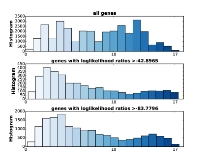
Figure S3: Histograms of estimated perturbation times for all the genes (upper panel), genes with loglikelihood ratios over -42.8965 (middle) and genes with loglikelihood ratios over -83.7796 (lower panel), respectively.

Genes were subsequently grouped into three groups: those whose perturbation time was $t<2.5$, those whose perturbation time was $2.5\leq t\leq 7$ and those perturbed $7<t<10$. In Tables LABEL:Tab:6 and LABEL:Tab:7 we indicate GO enrichment for genes filtered according to how dynamic their profiles were, whilst Tables LABEL:Tab:8 and LABEL:Tab:9 indicate GSEA. There is some evidence that early perturbed genes were again enriched for GO terms relating to signalling, and the PFAM Receptor kinase-like protein, although these terms were not apparent at the higher threshold. At the lower thresholds the presence of GO terms such as immune system process and defense response appear to show consistency with our earlier analysis based upon differentially expressed genes, with the higher threshold showing enrichment of other “response to …” type terms including, crucially, response to abscisic acid stimulus. Genes that were perturbed midway through the time series again show consistent enrichment for a variety of “response to ..” type terms, including response to bacterium, biotic stimulus, abiotic stimulus, and chemical stimulus. Late genes appear to be generally, and consistently enriched for GO terms and KEGG pathways related to chloroplasts and photosynthesis, as well as enrichment of related PFAM protein families. The general overlap of various terms, both at different likelihood thresholds, and for the different methods used for filtering, suggest that our approach has identified a consistent and genuine picture of the dynamics of plant-pathogen interactions.

S4.3 Distribution of Perturbation Times of Gene Ontologies and Pathways

Whilst the grouping of genes into early, middle and late genes well reflects the phases of bacterial infection, the calculation of perturbation times allows for the calculation of the distribution of particular Gene Ontology or Pathway terms. In turn this should allow the various terms to be ordered, producing a high resolution picture of the differences in processes that occur in Arabidopsis when infected with virulent DC3000 versus the disarmed mutant DC3000hrpA. To do so we calculated the perturbation times for all genes associated with a particular GO/Pathway term, and compared this distribution against that for all genes. Statistical significance was calculated using empirically corrected Kolmogorov-Smirnov (KS) tests and Kullback-Leibler (KL) divergence. The cumulative distribution function of all GO terms that are significantly perturbed using either KS or KL ($p<0.05$) are shown in heatmap form in Figures S4 - S15 , with significantly perturbed Pathways terms indicated in Fig. S16. For clarity, terms are ordered by the time at which $>50\%$ of associated genes are perturbed.

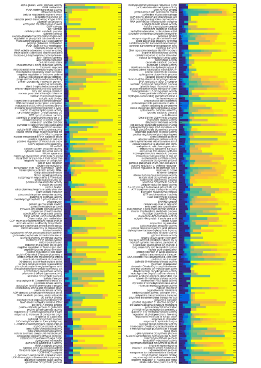
Figure S4: Temporal ordering of significantly perturbed GO terms.

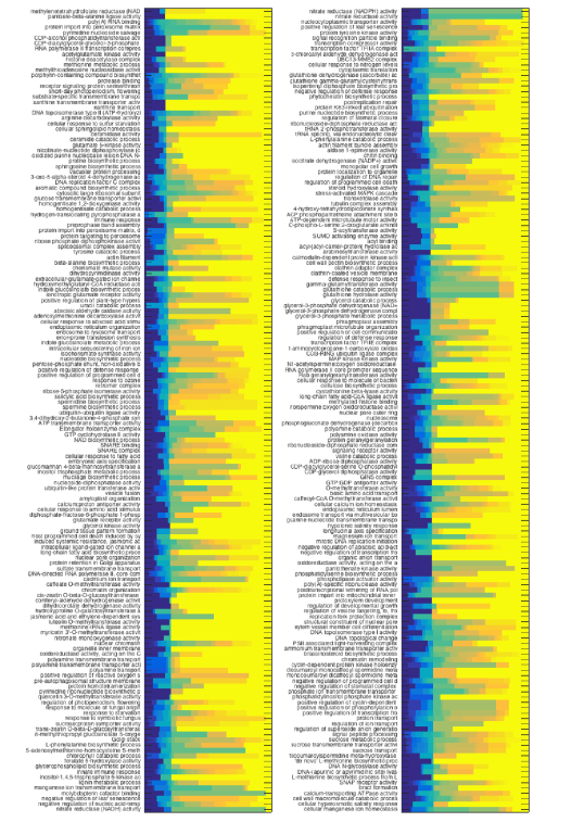
Figure S5: Temporal ordering of significantly perturbed GO terms.

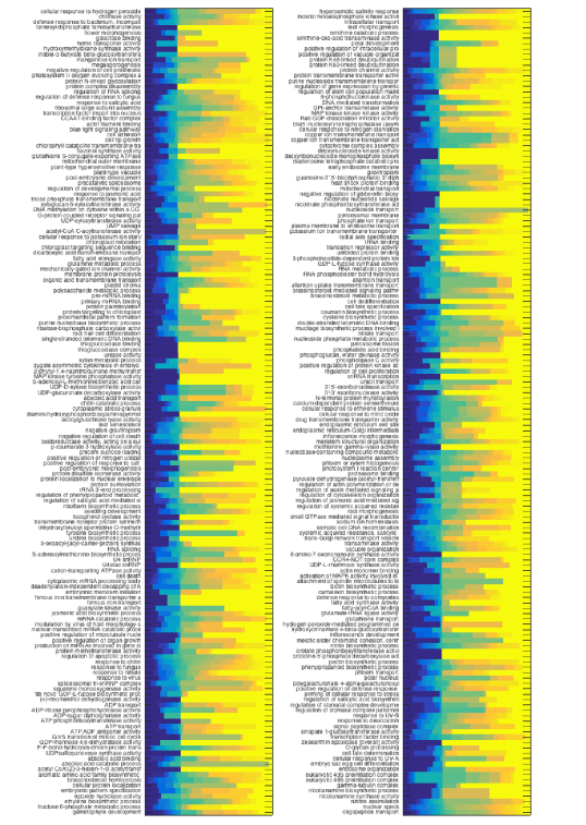
Figure S6: Temporal ordering of significantly perturbed GO terms.

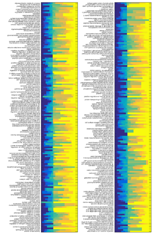
Figure S7: Temporal ordering of significantly perturbed GO terms.

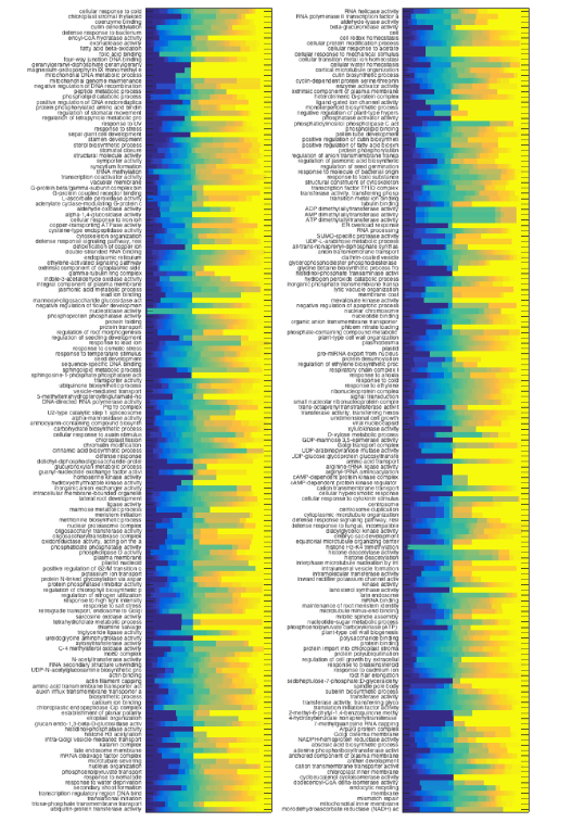
Figure S8: Temporal ordering of significantly perturbed GO terms.

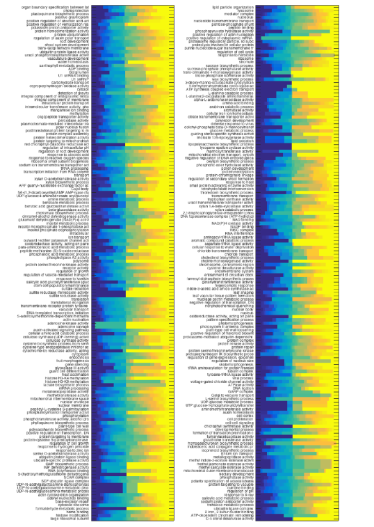
Figure S9: Temporal ordering of significantly perturbed GO terms.

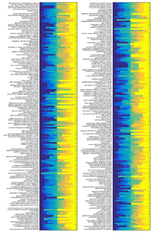
Figure S10: Temporal ordering of significantly perturbed GO terms.

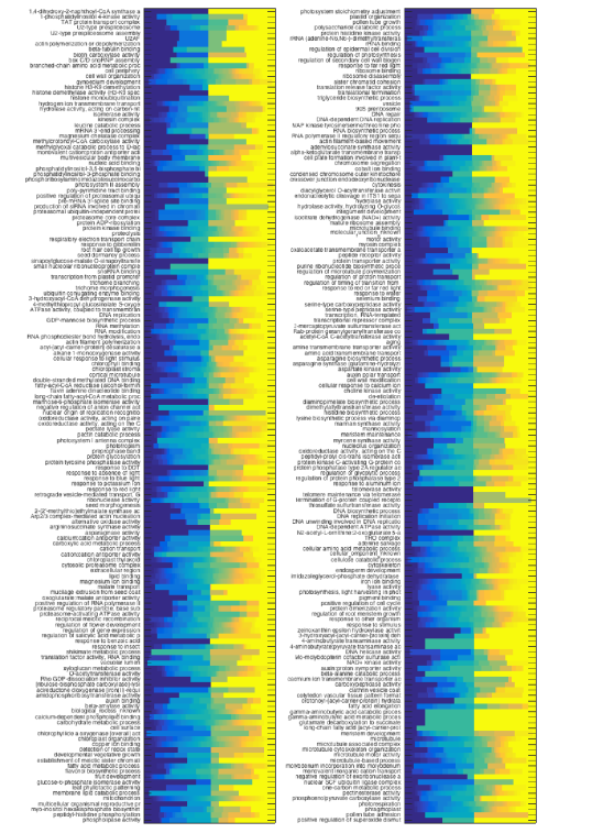
Figure S11: Temporal ordering of significantly perturbed GO terms.

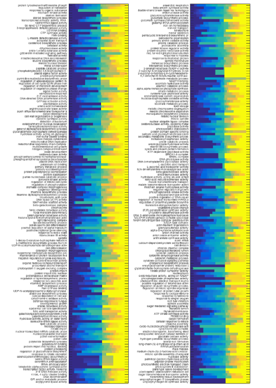
Figure S12: Temporal ordering of significantly perturbed GO terms.

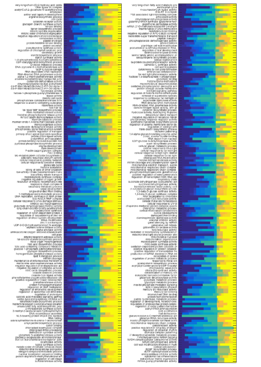
Figure S13: Temporal ordering of significantly perturbed GO terms.

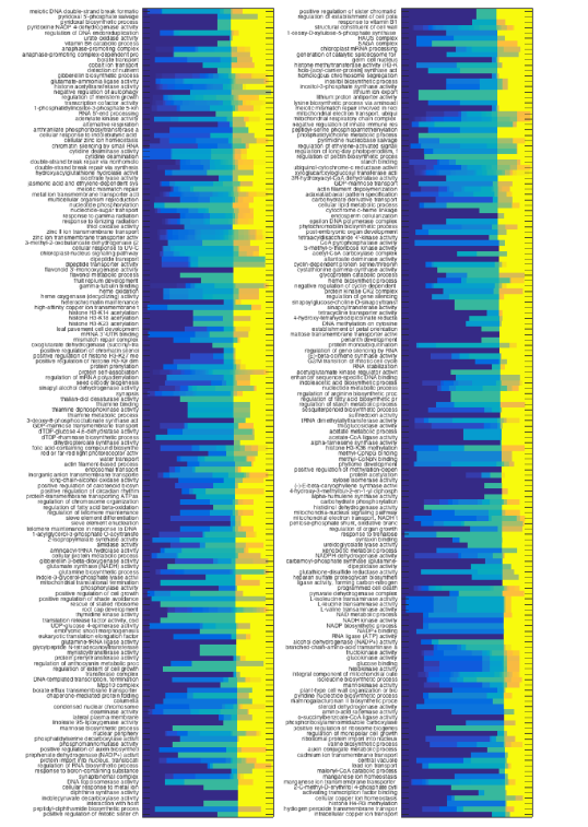
Figure S14: Temporal ordering of significantly perturbed GO terms.

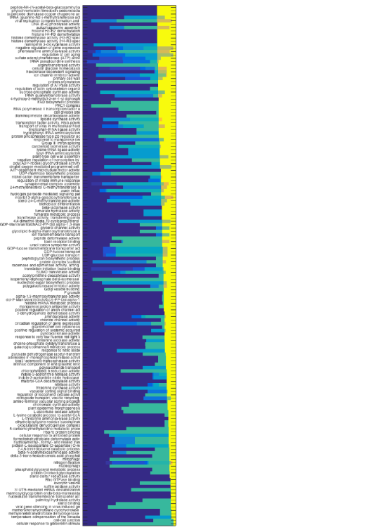
Figure S15: Temporal ordering of significantly perturbed GO terms.

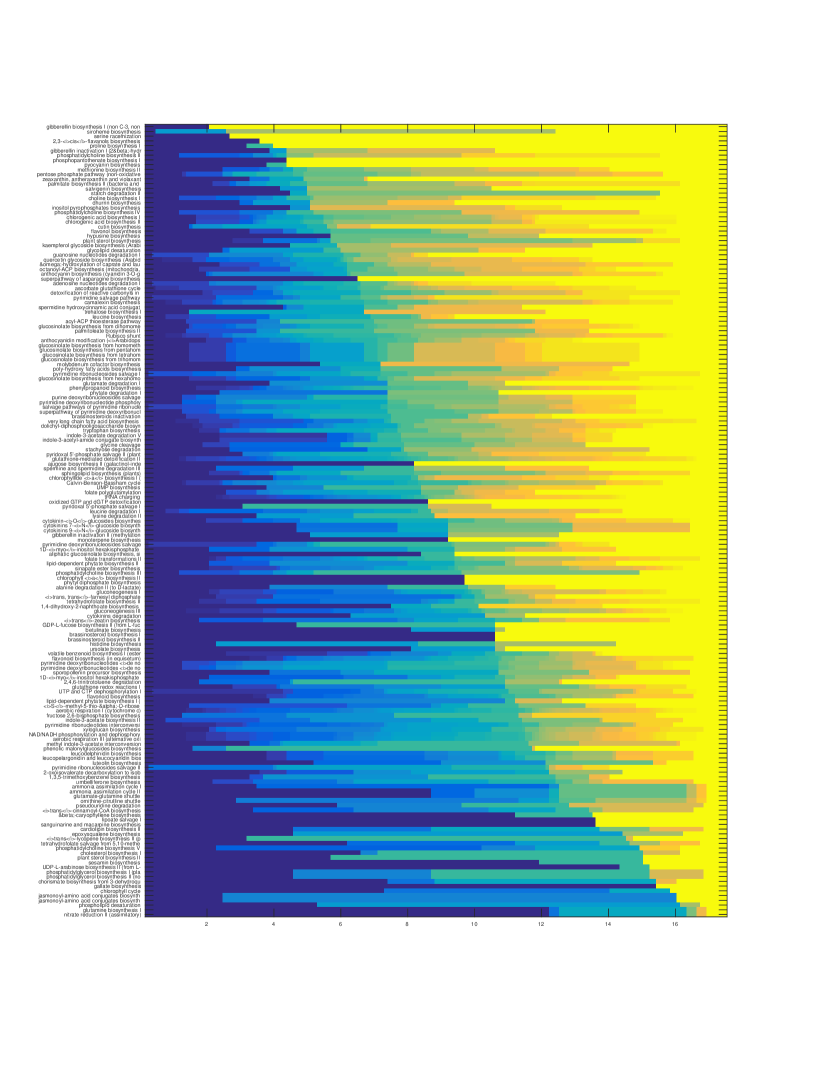
Figure S16: Temporal ordering of significantly perturbed Aracyc terms.

S5 Reference table of GO and AraCyc pathway terms

Finally in Table LABEL:Tab:11 we show the reference key to the Fig. 5 in the main text for GO and AraCyc pathway terms.

Table S2: GO analysis of genes perturbed between DC3000 and DC3000hrpA following identification of differentially expressed genes (log likelihood ratio $>4$)

PT	GO-ID	corr p-value	Description
$0\leq t<2.5$	3735	5.16E-15	structural constituent of ribosome
$0\leq t<2.5$	5622	3.12E-11	intracellular
$0\leq t<2.5$	5198	3.15E-11	structural molecule activity
$0\leq t<2.5$	44424	3.56E-11	intracellular part
$0\leq t<2.5$	5515	1.00E-09	protein binding
$0\leq t<2.5$	43229	1.35E-09	intracellular organelle
$0\leq t<2.5$	43226	1.35E-09	organelle
$0\leq t<2.5$	5623	1.55E-09	cell
$0\leq t<2.5$	44464	1.55E-09	cell part
$0\leq t<2.5$	43687	4.44E-08	post-translational protein modification
$0\leq t<2.5$	6464	8.29E-08	protein modification process
$0\leq t<2.5$	5886	2.20E-07	plasma membrane
$0\leq t<2.5$	16301	2.76E-07	kinase activity
$0\leq t<2.5$	16772	4.08E-07	transferase activity, transferring phosphorus-containing groups
$0\leq t<2.5$	5488	4.08E-07	binding
$0\leq t<2.5$	6796	4.08E-07	phosphate metabolic process
$0\leq t<2.5$	43231	4.08E-07	intracellular membrane-bounded organelle
$0\leq t<2.5$	43227	4.08E-07	membrane-bounded organelle
$0\leq t<2.5$	6793	4.08E-07	phosphorus metabolic process
$0\leq t<2.5$	6468	1.08E-06	protein amino acid phosphorylation
$0\leq t<2.5$	16310	1.38E-06	phosphorylation
$0\leq t<2.5$	5634	1.49E-06	nucleus
$0\leq t<2.5$	43412	2.94E-06	macromolecule modification
$0\leq t<2.5$	32991	3.46E-06	macromolecular complex
$0\leq t<2.5$	166	3.80E-06	nucleotide binding
$0\leq t<2.5$	43228	4.97E-06	non-membrane-bounded organelle
$0\leq t<2.5$	43232	4.97E-06	intracellular non-membrane-bounded organelle
$0\leq t<2.5$	16020	5.61E-06	membrane
$0\leq t<2.5$	9743	1.50E-05	response to carbohydrate stimulus
$0\leq t<2.5$	4672	1.63E-05	protein kinase activity
$0\leq t<2.5$	5840	1.86E-05	ribosome
$0\leq t<2.5$	31974	2.46E-05	membrane-enclosed lumen
$0\leq t<2.5$	10200	4.89E-05	response to chitin
$0\leq t<2.5$	5737	5.40E-05	cytoplasm
$0\leq t<2.5$	9987	5.61E-05	cellular process
$0\leq t<2.5$	44422	5.96E-05	organelle part
$0\leq t<2.5$	44446	7.68E-05	intracellular organelle part
$0\leq t<2.5$	16740	7.71E-05	transferase activity
$0\leq t<2.5$	31981	7.79E-05	nuclear lumen
$0\leq t<2.5$	22626	1.29E-04	cytosolic ribosome
$0\leq t<2.5$	5730	1.46E-04	nucleolus
$0\leq t<2.5$	44428	1.54E-04	nuclear part
$0\leq t<2.5$	43233	1.90E-04	organelle lumen
$0\leq t<2.5$	16773	2.50E-04	phosphotransferase activity, alcohol group as acceptor
$0\leq t<2.5$	44444	2.70E-04	cytoplasmic part
$0\leq t<2.5$	44445	2.91E-04	cytosolic part
$0\leq t<2.5$	50794	3.12E-04	regulation of cellular process
$0\leq t<2.5$	70013	3.12E-04	intracellular organelle lumen
$0\leq t<2.5$	23052	3.62E-04	signaling
$0\leq t<2.5$	4674	4.59E-04	protein serine/threonine kinase activity
$0\leq t<2.5$	51641	5.68E-04	cellular localization
$0\leq t<2.5$	5524	5.93E-04	ATP binding
$0\leq t<2.5$	5794	6.49E-04	Golgi apparatus
$0\leq t<2.5$	32559	6.53E-04	adenyl ribonucleotide binding
$0\leq t<2.5$	51649	7.81E-04	establishment of localization in cell
$0\leq t<2.5$	33279	8.28E-04	ribosomal subunit
$0\leq t<2.5$	50896	8.41E-04	response to stimulus
$0\leq t<2.5$	30554	9.94E-04	adenyl nucleotide binding
$0\leq t<2.5$	6950	1.04E-03	response to stress
$0\leq t<2.5$	1883	1.05E-03	purine nucleoside binding
$0\leq t<2.5$	1882	1.21E-03	nucleoside binding
$0\leq t<2.5$	50789	1.50E-03	regulation of biological process
$0\leq t<2.5$	30529	1.63E-03	ribonucleoprotein complex
$0\leq t<2.5$	71310	1.76E-03	cellular response to organic substance
$0\leq t<2.5$	10033	1.94E-03	response to organic substance
$0\leq t<2.5$	9595	2.23E-03	detection of biotic stimulus
$0\leq t<2.5$	9607	2.32E-03	response to biotic stimulus
$0\leq t<2.5$	44267	2.51E-03	cellular protein metabolic process
$0\leq t<2.5$	51707	2.66E-03	response to other organism
$0\leq t<2.5$	70887	2.85E-03	cellular response to chemical stimulus
$0\leq t<2.5$	6952	2.85E-03	defense response
$0\leq t<2.5$	22627	2.86E-03	cytosolic small ribosomal subunit
$0\leq t<2.5$	15935	2.86E-03	small ribosomal subunit
$0\leq t<2.5$	44260	3.46E-03	cellular macromolecule metabolic process
$0\leq t<2.5$	32553	3.49E-03	ribonucleotide binding
$0\leq t<2.5$	32555	3.49E-03	purine ribonucleotide binding
$0\leq t<2.5$	46907	3.64E-03	intracellular transport
$0\leq t<2.5$	51704	3.77E-03	multi-organism process
$0\leq t<2.5$	65004	3.85E-03	protein-DNA complex assembly
$0\leq t<2.5$	70727	3.85E-03	cellular macromolecule localization
$0\leq t<2.5$	17076	3.85E-03	purine nucleotide binding
$0\leq t<2.5$	43234	3.85E-03	protein complex
$0\leq t<2.5$	34621	3.85E-03	cellular macromolecular complex subunit organization
$0\leq t<2.5$	34622	3.85E-03	cellular macromolecular complex assembly
$0\leq t<2.5$	65007	5.02E-03	biological regulation
$0\leq t<2.5$	3674	5.79E-03	molecular function
$0\leq t<2.5$	44085	5.92E-03	cellular component biogenesis
$0\leq t<2.5$	5829	6.14E-03	cytosol
$0\leq t<2.5$	6333	6.28E-03	chromatin assembly or disassembly
$0\leq t<2.5$	34728	6.28E-03	nucleosome organization
$0\leq t<2.5$	6334	6.28E-03	nucleosome assembly
$0\leq t<2.5$	5057	6.87E-03	receptor signaling protein activity
$0\leq t<2.5$	2376	7.75E-03	immune system process
$0\leq t<2.5$	7166	8.10E-03	cell surface receptor linked signaling pathway
$0\leq t<2.5$	6886	8.10E-03	intracellular protein transport
$0\leq t<2.5$	6839	8.43E-03	mitochondrial transport
$0\leq t<2.5$	80008	8.89E-03	CUL4 RING ubiquitin ligase complex
$0\leq t<2.5$	31497	8.96E-03	chromatin assembly
$0\leq t<2.5$	34613	9.65E-03	cellular protein localization
$0\leq t<2.5$	23033	9.65E-03	signaling pathway
$2.5\leq t\leq 7$	16020	2.65E-16	membrane
$2.5\leq t\leq 7$	5886	7.10E-14	plasma membrane
$2.5\leq t\leq 7$	43231	2.68E-12	intracellular membrane-bounded organelle
$2.5\leq t\leq 7$	43227	2.68E-12	membrane-bounded organelle
$2.5\leq t\leq 7$	44464	1.01E-11	cell part
$2.5\leq t\leq 7$	5623	1.01E-11	cell
$2.5\leq t\leq 7$	50896	6.79E-11	response to stimulus
$2.5\leq t\leq 7$	5737	1.38E-10	cytoplasm
$2.5\leq t\leq 7$	44444	1.07E-09	cytoplasmic part
$2.5\leq t\leq 7$	43229	1.07E-09	intracellular organelle
$2.5\leq t\leq 7$	43226	1.07E-09	organelle
$2.5\leq t\leq 7$	5622	1.40E-09	intracellular
$2.5\leq t\leq 7$	44424	1.46E-09	intracellular part
$2.5\leq t\leq 7$	3824	6.90E-09	catalytic activity
$2.5\leq t\leq 7$	9628	3.00E-08	response to abiotic stimulus
$2.5\leq t\leq 7$	6950	6.95E-08	response to stress
$2.5\leq t\leq 7$	51707	1.02E-07	response to other organism
$2.5\leq t\leq 7$	9607	1.53E-07	response to biotic stimulus
$2.5\leq t\leq 7$	6970	5.02E-07	response to osmotic stress
$2.5\leq t\leq 7$	51704	5.14E-07	multi-organism process
$2.5\leq t\leq 7$	51234	5.71E-07	establishment of localization
$2.5\leq t\leq 7$	9651	7.61E-07	response to salt stress
$2.5\leq t\leq 7$	51179	7.61E-07	localization
$2.5\leq t\leq 7$	6810	9.72E-07	transport
$2.5\leq t\leq 7$	5515	1.27E-06	protein binding
$2.5\leq t\leq 7$	5783	6.18E-06	endoplasmic reticulum
$2.5\leq t\leq 7$	16740	6.18E-06	transferase activity
$2.5\leq t\leq 7$	5215	2.27E-05	transporter activity
$2.5\leq t\leq 7$	5773	2.27E-05	vacuole
$2.5\leq t\leq 7$	42221	2.31E-05	response to chemical stimulus
$2.5\leq t\leq 7$	44281	3.93E-05	small molecule metabolic process
$2.5\leq t\leq 7$	42742	6.39E-05	defense response to bacterium
$2.5\leq t\leq 7$	16311	1.81E-04	dephosphorylation
$2.5\leq t\leq 7$	6952	1.86E-04	defense response
$2.5\leq t\leq 7$	22857	1.87E-04	transmembrane transporter activity
$2.5\leq t\leq 7$	9617	2.45E-04	response to bacterium
$2.5\leq t\leq 7$	6470	2.97E-04	protein amino acid dephosphorylation
$2.5\leq t\leq 7$	44283	6.77E-04	small molecule biosynthetic process
$2.5\leq t\leq 7$	10033	1.11E-03	response to organic substance
$2.5\leq t\leq 7$	9536	1.39E-03	plastid
$2.5\leq t\leq 7$	22892	1.47E-03	substrate-specific transporter activity
$2.5\leq t\leq 7$	9507	1.49E-03	chloroplast
$2.5\leq t\leq 7$	22891	2.17E-03	substrate-specific transmembrane transporter activity
$2.5\leq t\leq 7$	16791	2.46E-03	phosphatase activity
$2.5\leq t\leq 7$	6575	2.75E-03	cellular amino acid derivative metabolic process
$2.5\leq t\leq 7$	6066	3.25E-03	alcohol metabolic process
$2.5\leq t\leq 7$	6519	4.13E-03	cellular amino acid and derivative metabolic process
$2.5\leq t\leq 7$	8287	4.59E-03	protein serine/threonine phosphatase complex
$2.5\leq t\leq 7$	42578	6.58E-03	phosphoric ester hydrolase activity
$2.5\leq t\leq 7$	42126	6.90E-03	nitrate metabolic process
$2.5\leq t\leq 7$	42128	6.90E-03	nitrate assimilation
$2.5\leq t\leq 7$	6518	7.20E-03	peptide metabolic process
$2.5\leq t\leq 7$	16772	7.35E-03	transferase activity, transferring phosphorus-containing groups
$2.5\leq t\leq 7$	6457	7.88E-03	protein folding
$2.5\leq t\leq 7$	5794	8.56E-03	Golgi apparatus
$2.5\leq t\leq 7$	9751	8.56E-03	response to salicylic acid stimulus
$2.5\leq t\leq 7$	267	8.56E-03	cell fraction
$2.5\leq t\leq 7$	9056	9.64E-03	catabolic process
$2.5\leq t\leq 7$	44282	9.64E-03	small molecule catabolic process
$t>7$	5737	1.23E-37	cytoplasm
$t>7$	9536	2.46E-36	plastid
$t>7$	9507	2.66E-34	chloroplast
$t>7$	44444	2.66E-34	cytoplasmic part
$t>7$	44435	7.01E-34	plastid part
$t>7$	44424	2.29E-31	intracellular part
$t>7$	43227	2.67E-31	membrane-bounded organelle
$t>7$	44434	2.67E-31	chloroplast part
$t>7$	43231	4.28E-31	intracellular membrane-bounded organelle
$t>7$	43226	7.57E-31	organelle
$t>7$	43229	1.37E-30	intracellular organelle
$t>7$	5622	1.41E-29	intracellular
$t>7$	44422	7.22E-20	organelle part
$t>7$	44446	1.40E-19	intracellular organelle part
$t>7$	9579	9.26E-18	thylakoid
$t>7$	9532	1.32E-17	plastid stroma
$t>7$	44436	2.25E-16	thylakoid part
$t>7$	42651	3.99E-16	thylakoid membrane
$t>7$	9526	6.19E-16	plastid envelope
$t>7$	34357	6.38E-16	photosynthetic membrane
$t>7$	9535	8.07E-16	chloroplast thylakoid membrane
$t>7$	55035	8.07E-16	plastid thylakoid membrane
$t>7$	9941	2.04E-15	chloroplast envelope
$t>7$	9534	2.44E-15	chloroplast thylakoid
$t>7$	31976	2.44E-15	plastid thylakoid
$t>7$	31984	3.30E-15	organelle subcompartment
$t>7$	9570	3.41E-15	chloroplast stroma
$t>7$	15979	9.14E-12	photosynthesis
$t>7$	5623	2.61E-11	cell
$t>7$	44464	2.61E-11	cell part
$t>7$	31967	4.87E-10	organelle envelope
$t>7$	31975	4.87E-10	envelope
$t>7$	16020	2.54E-07	membrane
$t>7$	9521	1.08E-06	photosystem
$t>7$	18130	1.17E-06	heterocycle biosynthetic process
$t>7$	19684	2.77E-06	photosynthesis, light reaction
$t>7$	8152	4.49E-06	metabolic process
$t>7$	51188	1.05E-05	cofactor biosynthetic process
$t>7$	48046	1.35E-05	apoplast
$t>7$	10287	1.70E-05	plastoglobule
$t>7$	33014	2.01E-05	tetrapyrrole biosynthetic process
$t>7$	44237	2.36E-05	cellular metabolic process
$t>7$	30076	2.49E-05	light-harvesting complex
$t>7$	6790	3.00E-05	sulfur metabolic process
$t>7$	3824	3.00E-05	catalytic activity
$t>7$	9110	3.00E-05	vitamin biosynthetic process
$t>7$	9523	3.50E-05	photosystem II
$t>7$	16168	3.50E-05	chlorophyll binding
$t>7$	6779	4.39E-05	porphyrin biosynthetic process
$t>7$	51186	5.49E-05	cofactor metabolic process
$t>7$	33013	6.46E-05	tetrapyrrole metabolic process
$t>7$	9791	6.59E-05	post-embryonic development
$t>7$	6766	7.63E-05	vitamin metabolic process
$t>7$	34641	8.46E-05	cellular nitrogen compound metabolic process
$t>7$	5739	9.47E-05	mitochondrion
$t>7$	15995	1.00E-04	chlorophyll biosynthetic process
$t>7$	9987	1.30E-04	cellular process
$t>7$	46148	1.46E-04	pigment biosynthetic process
$t>7$	16137	1.81E-04	glycoside metabolic process
$t>7$	6807	1.96E-04	nitrogen compound metabolic process
$t>7$	6778	2.06E-04	porphyrin metabolic process
$t>7$	16138	2.06E-04	glycoside biosynthetic process
$t>7$	19757	3.03E-04	glycosinolate metabolic process
$t>7$	19760	3.03E-04	glucosinolate metabolic process
$t>7$	16143	3.03E-04	S-glycoside metabolic process
$t>7$	19758	3.17E-04	glycosinolate biosynthetic process
$t>7$	19761	3.17E-04	glucosinolate biosynthetic process
$t>7$	16144	3.17E-04	S-glycoside biosynthetic process
$t>7$	42440	3.27E-04	pigment metabolic process
$t>7$	32501	4.15E-04	multicellular organismal process
$t>7$	31977	4.20E-04	thylakoid lumen
$t>7$	15994	4.48E-04	chlorophyll metabolic process
$t>7$	7275	4.96E-04	multicellular organismal development
$t>7$	32502	6.35E-04	developmental process
$t>7$	9543	6.35E-04	chloroplast thylakoid lumen
$t>7$	31978	6.35E-04	plastid thylakoid lumen
$t>7$	5576	7.81E-04	extracellular region
$t>7$	42180	8.12E-04	cellular ketone metabolic process
$t>7$	9295	8.39E-04	nucleoid
$t>7$	16874	9.37E-04	ligase activity
$t>7$	6520	9.60E-04	cellular amino acid metabolic process
$t>7$	43436	9.60E-04	oxoacid metabolic process
$t>7$	19752	9.60E-04	carboxylic acid metabolic process
$t>7$	6082	9.90E-04	organic acid metabolic process
$t>7$	44281	1.02E-03	small molecule metabolic process
$t>7$	9765	1.20E-03	photosynthesis, light harvesting
$t>7$	42364	1.42E-03	water-soluble vitamin biosynthetic process
$t>7$	10319	1.53E-03	stromule
$t>7$	9706	1.55E-03	chloroplast inner membrane
$t>7$	9658	1.77E-03	chloroplast organization
$t>7$	46483	1.84E-03	heterocycle metabolic process
$t>7$	10279	2.11E-03	indole-3-acetic acid amido synthetase activity
$t>7$	9654	2.63E-03	oxygen evolving complex
$t>7$	6418	2.63E-03	tRNA aminoacylation for protein translation
$t>7$	30095	2.72E-03	chloroplast photosystem II
$t>7$	9528	2.76E-03	plastid inner membrane
$t>7$	44271	2.85E-03	cellular nitrogen compound biosynthetic process
$t>7$	43038	2.85E-03	amino acid activation
$t>7$	43039	2.85E-03	tRNA aminoacylation
$t>7$	16875	2.85E-03	ligase activity, forming carbon-oxygen bonds
$t>7$	16876	2.85E-03	ligase activity, forming aminoacyl-tRNA and related compounds
$t>7$	4812	2.85E-03	aminoacyl-tRNA ligase activity
$t>7$	6091	2.86E-03	generation of precursor metabolites and energy
$t>7$	9657	3.03E-03	plastid organization
$t>7$	6767	3.03E-03	water-soluble vitamin metabolic process
$t>7$	9308	3.03E-03	amine metabolic process
$t>7$	48608	3.23E-03	reproductive structure development
$t>7$	229	3.41E-03	cytoplasmic chromosome
$t>7$	9508	3.41E-03	plastid chromosome
$t>7$	44106	3.65E-03	cellular amine metabolic process
$t>7$	6551	5.70E-03	leucine metabolic process
$t>7$	9628	5.87E-03	response to abiotic stimulus
$t>7$	44272	5.87E-03	sulfur compound biosynthetic process
$t>7$	48856	6.05E-03	anatomical structure development
$t>7$	70271	6.31E-03	protein complex biogenesis
$t>7$	6461	6.31E-03	protein complex assembly
$t>7$	44262	6.56E-03	cellular carbohydrate metabolic process
$t>7$	34637	6.72E-03	cellular carbohydrate biosynthetic process
$t>7$	15631	8.72E-03	tubulin binding
$t>7$	43234	8.86E-03	protein complex
$t>7$	3862	9.16E-03	3-isopropylmalate dehydrogenase activity
$t>7$	9606	9.38E-03	tropism

Table S3: GO analysis of genes perturbed between DC3000 and DC3000hrpA following identification of differentially expressed genes (log likelihood ratio $>10$)

PT	GO-ID	corr p-value	Description
$0\leq t<2.5$	5515	2.14E-09	protein binding
$0\leq t<2.5$	43687	2.22E-08	post-translational protein modification
$0\leq t<2.5$	6796	4.21E-08	phosphate metabolic process
$0\leq t<2.5$	6793	4.21E-08	phosphorus metabolic process
$0\leq t<2.5$	6468	1.15E-07	protein amino acid phosphorylation
$0\leq t<2.5$	6464	2.01E-07	protein modification process
$0\leq t<2.5$	16310	2.73E-07	phosphorylation
$0\leq t<2.5$	16772	8.28E-07	transferase activity, transferring phosphorus-containing groups
$0\leq t<2.5$	5488	8.28E-07	binding
$0\leq t<2.5$	43412	1.09E-06	macromolecule modification
$0\leq t<2.5$	16301	2.48E-06	kinase activity
$0\leq t<2.5$	5622	1.17E-05	intracellular
$0\leq t<2.5$	44424	1.50E-05	intracellular part
$0\leq t<2.5$	16740	1.65E-05	transferase activity
$0\leq t<2.5$	4672	6.16E-05	protein kinase activity
$0\leq t<2.5$	5623	6.16E-05	cell
$0\leq t<2.5$	44464	6.16E-05	cell part
$0\leq t<2.5$	166	7.33E-05	nucleotide binding
$0\leq t<2.5$	5886	9.72E-05	plasma membrane
$0\leq t<2.5$	23052	1.16E-04	signaling
$0\leq t<2.5$	43229	1.39E-04	intracellular organelle
$0\leq t<2.5$	43226	1.39E-04	organelle
$0\leq t<2.5$	34622	2.28E-04	cellular macromolecular complex assembly
$0\leq t<2.5$	34621	3.65E-04	cellular macromolecular complex subunit organization
$0\leq t<2.5$	6333	4.21E-04	chromatin assembly or disassembly
$0\leq t<2.5$	50794	8.66E-04	regulation of cellular process
$0\leq t<2.5$	43231	8.77E-04	intracellular membrane-bounded organelle
$0\leq t<2.5$	43227	8.77E-04	membrane-bounded organelle
$0\leq t<2.5$	5634	9.32E-04	nucleus
$0\leq t<2.5$	34728	1.11E-03	nucleosome organization
$0\leq t<2.5$	6334	1.11E-03	nucleosome assembly
$0\leq t<2.5$	16773	1.18E-03	phosphotransferase activity, alcohol group as acceptor
$0\leq t<2.5$	31497	1.55E-03	chromatin assembly
$0\leq t<2.5$	65003	1.55E-03	macromolecular complex assembly
$0\leq t<2.5$	4674	1.60E-03	protein serine/threonine kinase activity
$0\leq t<2.5$	22607	1.71E-03	cellular component assembly
$0\leq t<2.5$	65004	1.71E-03	protein-DNA complex assembly
$0\leq t<2.5$	9987	1.71E-03	cellular process
$0\leq t<2.5$	43933	1.96E-03	macromolecular complex subunit organization
$0\leq t<2.5$	5057	2.22E-03	receptor signaling protein activity
$0\leq t<2.5$	6323	2.26E-03	DNA packaging
$0\leq t<2.5$	71103	2.57E-03	DNA conformation change
$0\leq t<2.5$	16020	4.38E-03	membrane
$0\leq t<2.5$	50789	4.56E-03	regulation of biological process
$0\leq t<2.5$	6952	4.56E-03	defense response
$0\leq t<2.5$	9611	5.64E-03	response to wounding
$0\leq t<2.5$	23046	6.29E-03	signaling process
$0\leq t<2.5$	23060	6.29E-03	signal transmission
$0\leq t<2.5$	4702	6.32E-03	receptor signaling protein serine/threonine kinase activity
$0\leq t<2.5$	5524	6.32E-03	ATP binding
$0\leq t<2.5$	45087	6.32E-03	innate immune response
$0\leq t<2.5$	32559	6.69E-03	adenyl ribonucleotide binding
$0\leq t<2.5$	30554	6.83E-03	adenyl nucleotide binding
$0\leq t<2.5$	2376	6.96E-03	immune system process
$0\leq t<2.5$	1883	6.96E-03	purine nucleoside binding
$2.5\leq t\leq 7$	16020	1.59E-12	membrane
$2.5\leq t\leq 7$	50896	2.81E-09	response to stimulus
$2.5\leq t\leq 7$	5886	7.17E-08	plasma membrane
$2.5\leq t\leq 7$	44464	1.02E-06	cell part
$2.5\leq t\leq 7$	5623	1.02E-06	cell
$2.5\leq t\leq 7$	6950	4.76E-06	response to stress
$2.5\leq t\leq 7$	5737	6.82E-06	cytoplasm
$2.5\leq t\leq 7$	43231	6.82E-06	intracellular membrane-bounded organelle
$2.5\leq t\leq 7$	43227	6.82E-06	membrane-bounded organelle
$2.5\leq t\leq 7$	9628	1.13E-05	response to abiotic stimulus
$2.5\leq t\leq 7$	6970	1.41E-05	response to osmotic stress
$2.5\leq t\leq 7$	9651	2.39E-05	response to salt stress
$2.5\leq t\leq 7$	44424	3.78E-05	intracellular part
$2.5\leq t\leq 7$	42221	4.82E-05	response to chemical stimulus
$2.5\leq t\leq 7$	44444	4.82E-05	cytoplasmic part
$2.5\leq t\leq 7$	5622	4.82E-05	intracellular
$2.5\leq t\leq 7$	5215	8.29E-05	transporter activity
$2.5\leq t\leq 7$	5783	9.66E-05	endoplasmic reticulum
$2.5\leq t\leq 7$	22857	1.01E-04	transmembrane transporter activity
$2.5\leq t\leq 7$	43229	1.17E-04	intracellular organelle
$2.5\leq t\leq 7$	43226	1.17E-04	organelle
$2.5\leq t\leq 7$	51234	3.83E-04	establishment of localization
$2.5\leq t\leq 7$	10033	4.83E-04	response to organic substance
$2.5\leq t\leq 7$	51707	6.64E-04	response to other organism
$2.5\leq t\leq 7$	51179	8.14E-04	localization
$2.5\leq t\leq 7$	6810	8.14E-04	transport
$2.5\leq t\leq 7$	5773	1.00E-03	vacuole
$2.5\leq t\leq 7$	9607	1.00E-03	response to biotic stimulus
$2.5\leq t\leq 7$	5515	1.07E-03	protein binding
$2.5\leq t\leq 7$	3824	1.26E-03	catalytic activity
$2.5\leq t\leq 7$	22891	1.37E-03	substrate-specific transmembrane transporter activity
$2.5\leq t\leq 7$	42742	1.77E-03	defense response to bacterium
$2.5\leq t\leq 7$	22892	1.88E-03	substrate-specific transporter activity
$2.5\leq t\leq 7$	9617	2.06E-03	response to bacterium
$2.5\leq t\leq 7$	51704	2.45E-03	multi-organism process
$2.5\leq t\leq 7$	16740	3.10E-03	transferase activity
$2.5\leq t\leq 7$	15075	3.38E-03	ion transmembrane transporter activity
$2.5\leq t\leq 7$	9719	6.06E-03	response to endogenous stimulus
$2.5\leq t\leq 7$	9751	7.79E-03	response to salicylic acid stimulus
$2.5\leq t\leq 7$	42126	7.79E-03	nitrate metabolic process
$2.5\leq t\leq 7$	42128	7.79E-03	nitrate assimilation
$2.5\leq t\leq 7$	10817	9.12E-03	regulation of hormone levels
$t>7$	43231	1.52E-11	intracellular membrane-bounded organelle
$t>7$	43227	1.52E-11	membrane-bounded organelle
$t>7$	43229	2.22E-11	intracellular organelle
$t>7$	43226	2.22E-11	organelle
$t>7$	44424	2.22E-11	intracellular part
$t>7$	5622	5.45E-11	intracellular
$t>7$	5737	3.25E-10	cytoplasm
$t>7$	9536	4.81E-10	plastid
$t>7$	9507	2.01E-09	chloroplast
$t>7$	44444	2.19E-09	cytoplasmic part
$t>7$	44435	7.44E-09	plastid part
$t>7$	44434	6.43E-08	chloroplast part
$t>7$	19758	1.55E-06	glycosinolate biosynthetic process
$t>7$	19761	1.55E-06	glucosinolate biosynthetic process
$t>7$	16144	1.55E-06	S-glycoside biosynthetic process
$t>7$	9526	6.29E-06	plastid envelope
$t>7$	44446	2.21E-05	intracellular organelle part
$t>7$	44422	2.21E-05	organelle part
$t>7$	9941	2.21E-05	chloroplast envelope
$t>7$	19757	4.85E-05	glycosinolate metabolic process
$t>7$	19760	4.85E-05	glucosinolate metabolic process
$t>7$	16143	4.85E-05	S-glycoside metabolic process
$t>7$	9532	1.54E-04	plastid stroma
$t>7$	5623	2.02E-04	cell
$t>7$	44464	2.02E-04	cell part
$t>7$	44272	2.49E-04	sulfur compound biosynthetic process
$t>7$	9791	3.53E-04	post-embryonic development
$t>7$	6790	3.63E-04	sulfur metabolic process
$t>7$	16138	4.54E-04	glycoside biosynthetic process
$t>7$	9570	5.17E-04	chloroplast stroma
$t>7$	42651	8.27E-04	thylakoid membrane
$t>7$	9579	8.56E-04	thylakoid
$t>7$	34357	9.23E-04	photosynthetic membrane
$t>7$	31967	9.99E-04	organelle envelope
$t>7$	31975	9.99E-04	envelope
$t>7$	9535	1.24E-03	chloroplast thylakoid membrane
$t>7$	55035	1.24E-03	plastid thylakoid membrane
$t>7$	44436	1.78E-03	thylakoid part
$t>7$	3862	2.01E-03	3-isopropylmalate dehydrogenase activity
$t>7$	15979	2.23E-03	photosynthesis
$t>7$	9534	2.93E-03	chloroplast thylakoid
$t>7$	31976	2.93E-03	plastid thylakoid
$t>7$	48608	2.93E-03	reproductive structure development
$t>7$	31984	3.15E-03	organelle subcompartment
$t>7$	9523	5.35E-03	photosystem II
$t>7$	16137	5.80E-03	glycoside metabolic process
$t>7$	16709	6.12E-03	oxidoreductase activity, acting on paired donors
$t>7$	16020	6.18E-03	membrane
$t>7$	9521	6.70E-03	photosystem
$t>7$	15631	6.70E-03	tubulin binding
$t>7$	7275	6.92E-03	multicellular organismal development
$t>7$	8152	6.92E-03	metabolic process
$t>7$	34641	7.23E-03	cellular nitrogen compound metabolic process
$t>7$	32501	7.23E-03	multicellular organismal process
$t>7$	10287	7.23E-03	plastoglobule
$t>7$	48856	8.48E-03	anatomical structure development
$t>7$	32502	8.82E-03	developmental process
$t>7$	3006	9.78E-03	reproductive developmental process

Table S4: Genes that were perturbed between DC3000 and DC3000hrpA, and were also targeted by an effector from a range of pathogens in a yeast two-hybrid screen (Mukhtar et al., 2011).

Gene	Effector	Effector type	Likelihood ratio	Perturbation time
AT5G19990	HopBF1_Pla 107	Hop	11.8721721	1.02857142
AT4G38800	HopAF1_Pph 1448A	Hop	16.7558441	2.05714285
AT5G43700	HopH1_Psy B728A	Hop	8.40857712	2.05714285
AT3G46370	HopAB1_Pph 1448A	Hop	10.6853893	2.05714285
AT3G48550	HopR1-C-TERM_Pto DC3000	Hop	10.4462306	3.08571428
AT3G11720	HopM1_Pph 1448A	Hop	11.8544659	4.11428571
AT5G13810	HopX1_Pph 1448A	Hop	42.2497947	5.65714285
AT3G53350	HopAG1_Psy B728A	Hop	20.3038176	6.17142857
AT5G20000	HopBF1_Pla 107	Hop	4.61845378	10.2857142
AT5G42980	HARXL68	HAR	5.56181576	0
AT4G26450	HARXLL492	HAR	16.5541828	0
AT4G01090	HARXLL512	HAR	21.3353783	1.02857142
AT1G79430	HARXLL470_WACO9	HAR	33.2317206	1.54285714
AT3G16310	HARXLL493	HAR	74.7133852	1.54285714
AT1G67170	HARXLL470_WACO9	HAR	14.7482137	1.54285714
AT3G07780	HARXL21	HAR	17.9555558	2.05714285
AT3G54390	HARXLL470_WACO9	HAR	33.5467926	2.05714285
AT1G27300	HARXLL492	HAR	42.8363839	2.05714285
AT4G15140	HARXLL470_WACO9	HAR	10.5266792	2.05714285
AT3G60600	HARXLL492	HAR	28.5279074	2.57142857
AT4G09420	HARXL65	HAR	40.4810632	3.08571428
AT4G15545	HARXLL516_WACO9	HAR	39.794979	3.08571428
AT1G69370	HARXLL516_WACO9	HAR	14.6439695	3.6
AT5G14390	HARXL68	HAR	47.7737154	3.6
AT5G56250	HARXLL470_WACO9	HAR	34.0008537	3.6
AT5G56290	HARXLL73_2_WACO9	HAR	7.70505413	3.6
AT2G38750	HARXL45	HAR	17.7413833	4.11428571
AT2G34970	HARXLL429	HAR	15.8246298	4.11428571
AT5G22630	HARXLL73_2_WACO9	HAR	73.8224507	4.62857142
AT5G65210	HARXLL512	HAR	11.8164692	4.62857142
AT5G12230	HARXL44	HAR	22.4997621	4.62857142
AT4G35580	HARXLL492	HAR	30.7490491	5.65714285
AT3G44720	HARXLL73_2_WACO9	HAR	26.2067426	6.17142857
AT2G31260	HARXLL60	HAR	26.1511684	6.68571428
AT3G09980	HARXLL516_WACO9	HAR	28.3655226	6.68571428
AT3G49160	HARXLL445_2_WACO9	HAR	12.7060057	7.2
AT2G46420	HARXLL464	HAR	20.1845934	7.2
AT5G11980	HARXL73	HAR	4.51456878	7.71428571
AT5G02050	HARXL89	HAR	7.42209787	8.22857142
AT3G21490	HARXL44	HAR	4.13344692	11.3142857
AT5G60120	AvrPto1_Pla A7386	Avr	17.284651	0.51428571
AT4G02550	AvrB2_Pgy R0	Avr	35.0997065	1.02857142
AT3G17860	AvrPto1_Pla A7386	Avr	33.5111158	2.05714285
AT3G49570	AvrC_Xcc ATCC 33913	Avr	7.23033711	2.05714285
AT3G53410	AvrPto1_Pla 107	Avr	17.4074627	2.05714285
AT3G63210	AvrPto1_Pla A7386	Avr	8.74645208	3.08571428
AT3G17410	AvrB4-1_Pph 1448A	Avr	9.14014259	3.08571428
AT4G01920	AvrPto1_Pla A7386	Avr	4.92340704	4.11428571
AT2G35940	AvrPto1_Psy B728A	Avr	26.790228	4.62857142
AT1G14920	AvrB4-1_Pph 1448A	Avr	19.5449181	5.14285714
AT4G00710	AvrRpt2_Pto JL1065_CatalyticDead	Avr	22.8293957	6.17142857
AT4G11890	AvrPto1_Pla 107	Avr	15.1819962	9.25714285
AT5G57210	ATR13_NOKS1	ATR	36.6449542	1.02857142
AT2G23420	ATR1_MAKS9	ATR	18.4759372	1.02857142
AT1G22920	ATR1_ ASWA1	ATR	13.4331763	1.54285714
AT1G76850	ATR1_ ASWA1	ATR	9.59151322	1.54285714
AT3G02150	ATR1_ ASWA1	ATR	29.5597499	2.05714285
AT5G24660	ATR13_NOKS1	ATR	15.1526001	2.05714285
AT3G56270	ATR1_ ASWA1	ATR	5.10120681	2.05714285
AT3G50910	ATR13_NOKS1	ATR	36.3603035	2.05714285
AT2G23290	ATR13_NOKS1	ATR	25.5425875	2.57142857
AT1G63860	ATR13_HIND2	ATR	14.1501075	3.08571428
AT4G19700	ATR1_ ASWA1	ATR	20.4539952	3.6
AT3G25710	ATR1_ ASWA1	ATR	14.6250951	4.11428571
AT3G47620	ATR1_ ASWA1	ATR	10.5617836	4.11428571
AT3G54850	ATR13_NOKS1	ATR	13.6241798	5.14285714
AT5G22310	ATR13_NOKS1	ATR	4.90364133	5.14285714
AT4G34710	ATR13_NOKS1	ATR	7.05909499	5.65714285
AT1G69690	ATR1_ ASWA1	ATR	5.78419127	6.17142857
AT4G02590	ATR1_ ASWA1	ATR	4.93392493	8.22857142
AT5G51110	ATR1_ ASWA1	ATR	5.80816146	10.2857142

Table S5: Plant Gene Set Enrichment Analysis (GSEA) for genes differentially expressed between DC3000 and DC3000hrpA at a log likelihood ratio threshold $>4$

PT	corr p-value	Description
$0\leq t<2.5$	1.10E-08	Ribosome
$0\leq t<2.5$	2.75E-06	Receptor kinase-like protein family
$0\leq t<2.5$	4.48E-03	Confirmed target genes of transcription factor: HY5
$0\leq t<2.5$	4.48E-03	Confirmed and Unconfirmed target genes of transcription factor: HY5
$2.5\leq t\leq 7$	2.29E-05	Confirmed and Unconfirmed target genes of transcription factor: AtbHLH15
$2.5\leq t\leq 7$	1.60E-03	Confirmed target genes of transcription factor: AtbHLH15
$t>7$	1.98E-07	Metabolic pathways
$t>7$	7.80E-05	Photosynthesis - antenna proteins
$t>7$	7.93E-04	Biosynthesis of alkaloids derived from histidine and purine
$t>7$	0.0136	Chloroplast and Mitochondria gene families ,Chlorophyll a/b-binding protein family
$t>7$	0.0242	Ubiquitin mediated proteolysis
$t>7$	0.0296	Valine, leucine and isoleucine biosynthesis
$t>7$	0.0356	Photosynthesis
$t>7$	0.0464	chlorophyllide a biosynthesis I

Table S6: Plant Gene Set Enrichment Analysis (GSEA) for genes differentially expressed between DC3000 and DC3000hrpA at a log likelihood ratio threshold of $>10$

PT	corr p-value	Description
$0\leq t<2.5$	7.71E-09	Receptor kinase-like protein family
$0\leq t<2.5$	0.0293	Confirmed target genes of transcription factor: HY5
$0\leq t<2.5$	0.0293	Confirmed and Unconfirmed target genes of transcription factor: HY5
$0\leq t<2.5$	0.0431	Confirmed and Unconfirmed target genes of transcription factor: AtbHLH15
$2.5\leq t\leq 7$	3.64E-03	Confirmed and Unconfirmed target genes of transcription factor: AtbHLH15
$2.5\leq t\leq 7$	3.64E-03	Confirmed target genes of transcription factor: AtbHLH15
$t>7$	3.05E-03	Biosynthesis of alkaloids derived from histidine and purine
$t>7$	0.0227	Ubiquitin mediated proteolysis
$t>7$	0.0248	Glucosinolate biosynthesis
$t>7$	0.0264	Metabolic pathways

Table S7: GO analysis of genes perturbed between DC3000 and DC3000hrpA following identification of dynamically expressed genes with second most number of genes (log likelihood ratio of $>-83.7796$)

PT	GO-ID	corr p-value	Description
$0\leq t<2.5$	9987	2.91E-12	cellular process
$0\leq t<2.5$	44267	2.99E-10	cellular protein metabolic process
$0\leq t<2.5$	44260	1.39E-09	cellular macromolecule metabolic process
$0\leq t<2.5$	44237	3.64E-07	cellular metabolic process
$0\leq t<2.5$	19538	3.64E-07	protein metabolic process
$0\leq t<2.5$	43170	9.96E-07	macromolecule metabolic process
$0\leq t<2.5$	10467	1.13E-06	gene expression
$0\leq t<2.5$	43687	4.98E-06	post-translational protein modification
$0\leq t<2.5$	34645	4.98E-06	cellular macromolecule biosynthetic process
$0\leq t<2.5$	9059	6.99E-06	macromolecule biosynthetic process
$0\leq t<2.5$	6412	7.04E-06	translation
$0\leq t<2.5$	6464	8.54E-06	protein modification process
$0\leq t<2.5$	6796	1.64E-05	phosphate metabolic process
$0\leq t<2.5$	6793	1.64E-05	phosphorus metabolic process
$0\leq t<2.5$	6839	4.87E-05	mitochondrial transport
$0\leq t<2.5$	9743	7.97E-05	response to carbohydrate stimulus
$0\leq t<2.5$	16310	9.25E-05	phosphorylation
$0\leq t<2.5$	6468	1.33E-04	protein amino acid phosphorylation
$0\leq t<2.5$	10200	1.38E-04	response to chitin
$0\leq t<2.5$	43412	2.21E-04	macromolecule modification
$0\leq t<2.5$	44238	2.33E-04	primary metabolic process
$0\leq t<2.5$	51641	3.90E-04	cellular localization
$0\leq t<2.5$	70585	3.91E-04	protein localization in mitochondrion
$0\leq t<2.5$	6626	3.91E-04	protein targeting to mitochondrion
$0\leq t<2.5$	8152	4.39E-04	metabolic process
$0\leq t<2.5$	44249	4.96E-04	cellular biosynthetic process
$0\leq t<2.5$	6333	4.96E-04	chromatin assembly or disassembly
$0\leq t<2.5$	51649	6.57E-04	establishment of localization in cell
$0\leq t<2.5$	9058	1.45E-03	biosynthetic process
$0\leq t<2.5$	34728	2.11E-03	nucleosome organization
$0\leq t<2.5$	6334	2.11E-03	nucleosome assembly
$0\leq t<2.5$	50896	2.15E-03	response to stimulus
$0\leq t<2.5$	31497	3.12E-03	chromatin assembly
$0\leq t<2.5$	17038	3.22E-03	protein import
$0\leq t<2.5$	6952	3.23E-03	defense response
$0\leq t<2.5$	10033	3.23E-03	response to organic substance
$0\leq t<2.5$	2376	3.27E-03	immune system process
$0\leq t<2.5$	51179	3.27E-03	localization
$0\leq t<2.5$	65004	3.28E-03	protein-DNA complex assembly
$0\leq t<2.5$	51704	4.57E-03	multi-organism process
$0\leq t<2.5$	6323	4.74E-03	DNA packaging
$0\leq t<2.5$	6955	4.93E-03	immune response
$0\leq t<2.5$	6950	4.96E-03	response to stress
$0\leq t<2.5$	46907	5.29E-03	intracellular transport
$0\leq t<2.5$	51234	5.44E-03	establishment of localization
$0\leq t<2.5$	70727	5.85E-03	cellular macromolecule localization
$0\leq t<2.5$	9617	5.85E-03	response to bacterium
$0\leq t<2.5$	6605	6.65E-03	protein targeting
$0\leq t<2.5$	6810	6.65E-03	transport
$0\leq t<2.5$	42742	6.93E-03	defense response to bacterium
$0\leq t<2.5$	16043	7.09E-03	cellular component organization
$0\leq t<2.5$	6996	7.09E-03	organelle organization
$0\leq t<2.5$	51707	7.77E-03	response to other organism
$0\leq t<2.5$	6886	8.63E-03	intracellular protein transport
$0\leq t<2.5$	9607	8.82E-03	response to biotic stimulus
$0\leq t<2.5$	23052	8.88E-03	signaling
$0\leq t<2.5$	34613	9.20E-03	cellular protein localization
$0\leq t<2.5$	71103	9.78E-03	DNA conformation change
$0\leq t<2.5$	48583	9.79E-03	regulation of response to stimulus
$2.5\leq t\leq 7$	50896	2.95E-16	response to stimulus
$2.5\leq t\leq 7$	9628	6.00E-13	response to abiotic stimulus
$2.5\leq t\leq 7$	6950	1.60E-12	response to stress
$2.5\leq t\leq 7$	44281	4.00E-10	small molecule metabolic process
$2.5\leq t\leq 7$	42221	7.48E-10	response to chemical stimulus
$2.5\leq t\leq 7$	6970	2.01E-08	response to osmotic stress
$2.5\leq t\leq 7$	51707	2.01E-08	response to other organism
$2.5\leq t\leq 7$	9607	1.04E-07	response to biotic stimulus
$2.5\leq t\leq 7$	9651	2.79E-07	response to salt stress
$2.5\leq t\leq 7$	9611	5.51E-07	response to wounding
$2.5\leq t\leq 7$	51234	1.08E-06	establishment of localization
$2.5\leq t\leq 7$	6810	1.86E-06	transport
$2.5\leq t\leq 7$	51179	2.09E-06	localization
$2.5\leq t\leq 7$	44283	5.33E-06	small molecule biosynthetic process
$2.5\leq t\leq 7$	51704	1.09E-05	multi-organism process
$2.5\leq t\leq 7$	6519	2.68E-05	cellular amino acid and derivative metabolic process
$2.5\leq t\leq 7$	6575	2.86E-05	cellular amino acid derivative metabolic process
$2.5\leq t\leq 7$	44271	2.86E-05	cellular nitrogen compound biosynthetic process
$2.5\leq t\leq 7$	10033	2.86E-05	response to organic substance
$2.5\leq t\leq 7$	6811	5.49E-05	ion transport
$2.5\leq t\leq 7$	9266	5.74E-05	response to temperature stimulus
$2.5\leq t\leq 7$	6694	1.00E-04	steroid biosynthetic process
$2.5\leq t\leq 7$	42742	1.06E-04	defense response to bacterium
$2.5\leq t\leq 7$	10035	1.12E-04	response to inorganic substance
$2.5\leq t\leq 7$	9617	1.86E-04	response to bacterium
$2.5\leq t\leq 7$	9414	2.71E-04	response to water deprivation
$2.5\leq t\leq 7$	10038	2.87E-04	response to metal ion
$2.5\leq t\leq 7$	6952	4.81E-04	defense response
$2.5\leq t\leq 7$	9056	5.06E-04	catabolic process
$2.5\leq t\leq 7$	9415	7.18E-04	response to water
$2.5\leq t\leq 7$	51186	1.15E-03	cofactor metabolic process
$2.5\leq t\leq 7$	46686	1.26E-03	response to cadmium ion
$2.5\leq t\leq 7$	6865	1.28E-03	amino acid transport
$2.5\leq t\leq 7$	9409	1.42E-03	response to cold
$2.5\leq t\leq 7$	9719	1.43E-03	response to endogenous stimulus
$2.5\leq t\leq 7$	15837	1.49E-03	amine transport
$2.5\leq t\leq 7$	46942	2.09E-03	carboxylic acid transport
$2.5\leq t\leq 7$	15849	2.09E-03	organic acid transport
$2.5\leq t\leq 7$	9620	2.13E-03	response to fungus
$2.5\leq t\leq 7$	6749	2.28E-03	glutathione metabolic process
$2.5\leq t\leq 7$	55086	2.29E-03	nucleobase, nucleoside and nucleotide metabolic process
$2.5\leq t\leq 7$	6725	2.70E-03	cellular aromatic compound metabolic process
$2.5\leq t\leq 7$	6733	2.81E-03	oxidoreduction coenzyme metabolic process
$2.5\leq t\leq 7$	8202	2.81E-03	steroid metabolic process
$2.5\leq t\leq 7$	6082	3.21E-03	organic acid metabolic process
$2.5\leq t\leq 7$	9753	3.28E-03	response to jasmonic acid stimulus
$2.5\leq t\leq 7$	19362	3.28E-03	pyridine nucleotide metabolic process
$2.5\leq t\leq 7$	42180	3.32E-03	cellular ketone metabolic process
$2.5\leq t\leq 7$	6518	3.34E-03	peptide metabolic process
$2.5\leq t\leq 7$	16126	3.34E-03	sterol biosynthetic process
$2.5\leq t\leq 7$	6066	3.43E-03	alcohol metabolic process
$2.5\leq t\leq 7$	6732	3.57E-03	coenzyme metabolic process
$2.5\leq t\leq 7$	46496	3.57E-03	nicotinamide nucleotide metabolic process
$2.5\leq t\leq 7$	43436	3.92E-03	oxoacid metabolic process
$2.5\leq t\leq 7$	19752	3.92E-03	carboxylic acid metabolic process
$2.5\leq t\leq 7$	42126	4.05E-03	nitrate metabolic process
$2.5\leq t\leq 7$	42128	4.05E-03	nitrate assimilation
$2.5\leq t\leq 7$	8333	4.95E-03	endosome to lysosome transport
$2.5\leq t\leq 7$	7041	4.95E-03	lysosomal transport
$2.5\leq t\leq 7$	9640	4.95E-03	photomorphogenesis
$2.5\leq t\leq 7$	31407	5.30E-03	oxylipin metabolic process
$2.5\leq t\leq 7$	6091	5.30E-03	generation of precursor metabolites and energy
$2.5\leq t\leq 7$	16052	5.78E-03	carbohydrate catabolic process
$2.5\leq t\leq 7$	19748	5.78E-03	secondary metabolic process
$2.5\leq t\leq 7$	6812	7.88E-03	cation transport
$2.5\leq t\leq 7$	19438	8.06E-03	aromatic compound biosynthetic process
$2.5\leq t\leq 7$	9117	8.06E-03	nucleotide metabolic process
$2.5\leq t\leq 7$	6753	8.06E-03	nucleoside phosphate metabolic process
$2.5\leq t\leq 7$	8610	8.06E-03	lipid biosynthetic process
$2.5\leq t\leq 7$	42398	8.06E-03	cellular amino acid derivative biosynthetic process
$2.5\leq t\leq 7$	19359	8.06E-03	nicotinamide nucleotide biosynthetic process
$2.5\leq t\leq 7$	6820	8.06E-03	anion transport
$2.5\leq t\leq 7$	44275	8.06E-03	cellular carbohydrate catabolic process
$2.5\leq t\leq 7$	6790	9.13E-03	sulfur metabolic process
$2.5\leq t\leq 7$	44273	9.60E-03	sulfur compound catabolic process
$7>t\leq 10$	8152	1.66E-12	metabolic process
$7>t\leq 10$	15979	1.93E-11	photosynthesis
$7>t\leq 10$	9987	3.06E-10	cellular process
$7>t\leq 10$	44237	8.63E-10	cellular metabolic process
$7>t\leq 10$	42180	6.62E-09	cellular ketone metabolic process
$7>t\leq 10$	44281	9.52E-09	small molecule metabolic process
$7>t\leq 10$	43436	1.65E-08	oxoacid metabolic process
$7>t\leq 10$	19752	1.65E-08	carboxylic acid metabolic process
$7>t\leq 10$	6082	1.65E-08	organic acid metabolic process
$7>t\leq 10$	44271	1.09E-07	cellular nitrogen compound biosynthetic process
$7>t\leq 10$	6520	1.77E-07	cellular amino acid metabolic process
$7>t\leq 10$	34641	3.37E-07	cellular nitrogen compound metabolic process
$7>t\leq 10$	18130	1.06E-06	heterocycle biosynthetic process
$7>t\leq 10$	51186	2.52E-06	cofactor metabolic process
$7>t\leq 10$	6807	2.83E-06	nitrogen compound metabolic process
$7>t\leq 10$	44106	3.51E-06	cellular amine metabolic process
$7>t\leq 10$	19684	2.40E-05	photosynthesis, light reaction
$7>t\leq 10$	46394	2.48E-05	carboxylic acid biosynthetic process
$7>t\leq 10$	16053	2.48E-05	organic acid biosynthetic process
$7>t\leq 10$	9308	3.27E-05	amine metabolic process
$7>t\leq 10$	51188	4.36E-05	cofactor biosynthetic process
$7>t\leq 10$	8652	4.36E-05	cellular amino acid biosynthetic process
$7>t\leq 10$	44283	6.43E-05	small molecule biosynthetic process
$7>t\leq 10$	42440	6.49E-05	pigment metabolic process
$7>t\leq 10$	9790	8.89E-05	embryonic development
$7>t\leq 10$	6519	1.09E-04	cellular amino acid and derivative metabolic process
$7>t\leq 10$	33014	1.16E-04	tetrapyrrole biosynthetic process
$7>t\leq 10$	9657	1.16E-04	plastid organization
$7>t\leq 10$	46686	1.30E-04	response to cadmium ion
$7>t\leq 10$	42221	1.43E-04	response to chemical stimulus
$7>t\leq 10$	9791	1.43E-04	post-embryonic development
$7>t\leq 10$	33013	2.17E-04	tetrapyrrole metabolic process
$7>t\leq 10$	9793	3.28E-04	embryonic development ending in seed dormancy
$7>t\leq 10$	6418	3.28E-04	tRNA aminoacylation for protein translation
$7>t\leq 10$	46483	3.51E-04	heterocycle metabolic process
$7>t\leq 10$	9309	3.52E-04	amine biosynthetic process
$7>t\leq 10$	43038	3.79E-04	amino acid activation
$7>t\leq 10$	43039	3.79E-04	tRNA aminoacylation
$7>t\leq 10$	9651	4.19E-04	response to salt stress
$7>t\leq 10$	6778	4.62E-04	porphyrin metabolic process
$7>t\leq 10$	6970	4.94E-04	response to osmotic stress
$7>t\leq 10$	9058	5.65E-04	biosynthetic process
$7>t\leq 10$	6779	6.02E-04	porphyrin biosynthetic process
$7>t\leq 10$	50896	6.07E-04	response to stimulus
$7>t\leq 10$	9628	6.21E-04	response to abiotic stimulus
$7>t\leq 10$	48608	7.18E-04	reproductive structure development
$7>t\leq 10$	48316	7.29E-04	seed development
$7>t\leq 10$	46148	8.52E-04	pigment biosynthetic process
$7>t\leq 10$	44249	8.68E-04	cellular biosynthetic process
$7>t\leq 10$	10154	8.78E-04	fruit development
$7>t\leq 10$	10035	9.47E-04	response to inorganic substance
$7>t\leq 10$	44262	1.11E-03	cellular carbohydrate metabolic process
$7>t\leq 10$	6399	1.11E-03	tRNA metabolic process
$7>t\leq 10$	9056	1.62E-03	catabolic process
$7>t\leq 10$	16137	1.69E-03	glycoside metabolic process
$7>t\leq 10$	32501	2.16E-03	multicellular organismal process
$7>t\leq 10$	6766	2.56E-03	vitamin metabolic process
$7>t\leq 10$	32502	2.61E-03	developmental process
$7>t\leq 10$	9110	3.28E-03	vitamin biosynthetic process
$7>t\leq 10$	6790	3.34E-03	sulfur metabolic process
$7>t\leq 10$	9737	3.36E-03	response to abscisic acid stimulus
$7>t\leq 10$	16070	3.40E-03	RNA metabolic process
$7>t\leq 10$	9658	3.42E-03	chloroplast organization
$7>t\leq 10$	10038	3.42E-03	response to metal ion
$7>t\leq 10$	6091	3.53E-03	generation of precursor metabolites and energy
$7>t\leq 10$	7275	4.05E-03	multicellular organismal development
$7>t\leq 10$	19758	4.13E-03	glycosinolate biosynthetic process
$7>t\leq 10$	19761	4.13E-03	glucosinolate biosynthetic process
$7>t\leq 10$	16144	4.13E-03	S-glycoside biosynthetic process
$7>t\leq 10$	16138	4.18E-03	glycoside biosynthetic process
$7>t\leq 10$	31163	4.29E-03	metallo-sulfur cluster assembly
$7>t\leq 10$	16226	4.29E-03	iron-sulfur cluster assembly
$7>t\leq 10$	34285	4.45E-03	response to disaccharide stimulus
$7>t\leq 10$	16043	4.55E-03	cellular component organization
$7>t\leq 10$	3006	4.56E-03	reproductive developmental process
$7>t\leq 10$	5975	4.70E-03	carbohydrate metabolic process
$7>t\leq 10$	31399	5.58E-03	regulation of protein modification process
$7>t\leq 10$	15995	5.65E-03	chlorophyll biosynthetic process
$7>t\leq 10$	9765	5.68E-03	photosynthesis, light harvesting
$7>t\leq 10$	16109	5.68E-03	tetraterpenoid biosynthetic process
$7>t\leq 10$	16117	5.68E-03	carotenoid biosynthetic process
$7>t\leq 10$	10033	7.20E-03	response to organic substance
$7>t\leq 10$	22414	7.56E-03	reproductive process
$7>t\leq 10$	19748	7.69E-03	secondary metabolic process
$7>t\leq 10$	16051	7.83E-03	carbohydrate biosynthetic process
$7>t\leq 10$	19757	7.83E-03	glycosinolate metabolic process
$7>t\leq 10$	19760	7.83E-03	glucosinolate metabolic process
$7>t\leq 10$	16143	7.83E-03	S-glycoside metabolic process
$7>t\leq 10$	15994	7.96E-03	chlorophyll metabolic process
$7>t\leq 10$	44248	7.98E-03	cellular catabolic process
$7>t\leq 10$	44272	8.29E-03	sulfur compound biosynthetic process
$7>t\leq 10$	6551	9.13E-03	leucine metabolic process

Table S8: GO analysis of genes perturbed between DC3000 and DC3000hrpA following identification of dynamically expressed genes with fewest number of genes (log likelihood ratio $>-42.8965$)

PT	GO-ID	corr p-value	Description
$0\leq t<2.5$	44267	9.27E-09	cellular protein metabolic process
$0\leq t<2.5$	6412	2.72E-08	translation
$0\leq t<2.5$	10467	1.02E-07	gene expression
$0\leq t<2.5$	44260	1.49E-07	cellular macromolecule metabolic process
$0\leq t<2.5$	19538	3.22E-07	protein metabolic process
$0\leq t<2.5$	9987	1.42E-06	cellular process
$0\leq t<2.5$	34645	1.42E-06	cellular macromolecule biosynthetic process
$0\leq t<2.5$	9059	1.49E-06	macromolecule biosynthetic process
$0\leq t<2.5$	44237	1.49E-06	cellular metabolic process
$0\leq t<2.5$	43170	3.23E-06	macromolecule metabolic process
$0\leq t<2.5$	44249	5.71E-05	cellular biosynthetic process
$0\leq t<2.5$	44238	6.74E-05	primary metabolic process
$0\leq t<2.5$	8152	1.94E-04	metabolic process
$0\leq t<2.5$	9058	2.24E-04	biosynthetic process
$0\leq t<2.5$	42221	1.76E-03	response to chemical stimulus
$0\leq t<2.5$	9737	3.28E-03	response to abscisic acid stimulus
$0\leq t<2.5$	10033	6.11E-03	response to organic substance
$0\leq t<2.5$	9415	8.78E-03	response to water
$0\leq t<2.5$	9719	9.55E-03	response to endogenous stimulus
$2.5\leq t\leq 7$	50896	1.57E-15	response to stimulus
$2.5\leq t\leq 7$	9628	1.26E-11	response to abiotic stimulus
$2.5\leq t\leq 7$	6950	3.22E-09	response to stress
$2.5\leq t\leq 7$	51704	2.52E-08	multi-organism process
$2.5\leq t\leq 7$	51707	2.52E-08	response to other organism
$2.5\leq t\leq 7$	9607	9.67E-08	response to biotic stimulus
$2.5\leq t\leq 7$	51179	2.28E-06	localization
$2.5\leq t\leq 7$	51234	2.95E-06	establishment of localization
$2.5\leq t\leq 7$	6810	6.11E-06	transport
$2.5\leq t\leq 7$	42221	4.97E-05	response to chemical stimulus
$2.5\leq t\leq 7$	44281	2.34E-04	small molecule metabolic process
$2.5\leq t\leq 7$	9314	3.79E-04	response to radiation
$2.5\leq t\leq 7$	48193	3.79E-04	Golgi vesicle transport
$2.5\leq t\leq 7$	6970	3.93E-04	response to osmotic stress
$2.5\leq t\leq 7$	32502	4.39E-04	developmental process
$2.5\leq t\leq 7$	9416	4.54E-04	response to light stimulus
$2.5\leq t\leq 7$	6952	4.62E-04	defense response
$2.5\leq t\leq 7$	32501	4.62E-04	multicellular organismal process
$2.5\leq t\leq 7$	6575	7.48E-04	cellular amino acid derivative metabolic process
$2.5\leq t\leq 7$	7275	1.06E-03	multicellular organismal development
$2.5\leq t\leq 7$	10033	1.84E-03	response to organic substance
$2.5\leq t\leq 7$	6457	2.63E-03	protein folding
$2.5\leq t\leq 7$	9117	2.76E-03	nucleotide metabolic process
$2.5\leq t\leq 7$	6753	2.76E-03	nucleoside phosphate metabolic process
$2.5\leq t\leq 7$	71214	3.26E-03	cellular response to abiotic stimulus
$2.5\leq t\leq 7$	44283	3.41E-03	small molecule biosynthetic process
$2.5\leq t\leq 7$	6464	3.98E-03	protein modification process
$2.5\leq t\leq 7$	9651	4.04E-03	response to salt stress
$2.5\leq t\leq 7$	9165	4.48E-03	nucleotide biosynthetic process
$2.5\leq t\leq 7$	9617	4.65E-03	response to bacterium
$2.5\leq t\leq 7$	9620	5.69E-03	response to fungus
$2.5\leq t\leq 7$	16043	5.69E-03	cellular component organization
$2.5\leq t\leq 7$	55086	6.96E-03	nucleobase, nucleoside and nucleotide metabolic process
$7>t\leq 10$	15979	6.44E-16	photosynthesis
$7>t\leq 10$	8152	2.59E-13	metabolic process
$7>t\leq 10$	19684	4.51E-10	photosynthesis, light reaction
$7>t\leq 10$	44237	1.09E-08	cellular metabolic process
$7>t\leq 10$	6091	6.54E-06	generation of precursor metabolites and energy
$7>t\leq 10$	46686	3.20E-05	response to cadmium ion
$7>t\leq 10$	9987	3.52E-05	cellular process
$7>t\leq 10$	10038	1.58E-04	response to metal ion
$7>t\leq 10$	44281	1.58E-04	small molecule metabolic process
$7>t\leq 10$	9628	1.58E-04	response to abiotic stimulus
$7>t\leq 10$	9767	2.12E-04	photosynthetic electron transport chain
$7>t\leq 10$	9058	5.18E-04	biosynthetic process
$7>t\leq 10$	44249	6.89E-04	cellular biosynthetic process
$7>t\leq 10$	10035	7.68E-04	response to inorganic substance
$7>t\leq 10$	48511	8.22E-04	rhythmic process
$7>t\leq 10$	7623	8.22E-04	circadian rhythm
$7>t\leq 10$	9765	1.02E-03	photosynthesis, light harvesting
$7>t\leq 10$	10114	1.40E-03	response to red light
$7>t\leq 10$	50896	1.99E-03	response to stimulus
$7>t\leq 10$	10218	2.37E-03	response to far red light
$7>t\leq 10$	44271	2.63E-03	cellular nitrogen compound biosynthetic process
$7>t\leq 10$	51186	3.04E-03	cofactor metabolic process
$7>t\leq 10$	9773	3.27E-03	photosynthetic electron transport in photosystem I
$7>t\leq 10$	55114	3.27E-03	oxidation reduction
$7>t\leq 10$	42180	4.73E-03	cellular ketone metabolic process
$7>t\leq 10$	42440	4.73E-03	pigment metabolic process
$7>t\leq 10$	42360	4.73E-03	vitamin E metabolic process
$7>t\leq 10$	10189	4.73E-03	vitamin E biosynthetic process
$7>t\leq 10$	9637	5.10E-03	response to blue light
$7>t\leq 10$	30163	5.41E-03	protein catabolic process
$7>t\leq 10$	46148	7.33E-03	pigment biosynthetic process
$7>t\leq 10$	43436	7.33E-03	oxoacid metabolic process
$7>t\leq 10$	19752	7.33E-03	carboxylic acid metabolic process
$7>t\leq 10$	6082	7.33E-03	organic acid metabolic process
$7>t\leq 10$	22900	7.95E-03	electron transport chain
$7>t\leq 10$	9057	8.13E-03	macromolecule catabolic process
$7>t\leq 10$	42221	8.99E-03	response to chemical stimulus
$7>t\leq 10$	51188	9.60E-03	cofactor biosynthetic process
$7>t\leq 10$	44257	9.60E-03	cellular protein catabolic process
$7>t\leq 10$	15994	9.60E-03	chlorophyll metabolic process
$7>t\leq 10$	6778	9.90E-03	porphyrin metabolic process

Table S9: Plant Gene Set Enrichment Analysis (GSEA) for genes dynamically expressed with a log likelihood ratio $>-83.7796$

PT	corr p-value	Description
$0\leq t<2.5$	2.79E-32	Ribosome
$0\leq t<2.5$	4.79E-03	Receptor kinase-like protein family
$0\leq t<2.5$	0.0343	Spliceosome
$2.5\leq t\leq 7$	9.46E-05	Confirmed and Unconfirmed target genes of transcription factor: AtbHLH15
$2.5\leq t\leq 7$	6.19E-03	Metabolic pathways
$7>t\leq 10$	4.56E-15	Metabolic pathways
$7>t\leq 10$	1.51E-05	Biosynthesis of alkaloids derived from histidine and purine
$7>t\leq 10$	9.45E-05	Biosynthesis of alkaloids derived from shikimate pathway
$7>t\leq 10$	1.54E-04	Biosynthesis of alkaloids derived from ornithine, lysine and nicotinic acid
$7>t\leq 10$	7.87E-04	Aminoacyl-tRNA biosynthesis
$7>t\leq 10$	1.41E-03	Biosynthesis of plant hormones
$7>t\leq 10$	1.41E-03	Biosynthesis of phenylpropanoids
$7>t\leq 10$	1.41E-03	Valine, leucine and isoleucine biosynthesis
$7>t\leq 10$	2.32E-03	Carbon fixation in photosynthetic organisms
$7>t\leq 10$	2.32E-03	Photosynthesis - antenna proteins
$7>t\leq 10$	0.0115	Biosynthesis of alkaloids derived from terpenoid and polyketide
$7>t\leq 10$	0.0189	Biosynthesis of terpenoids and steroids
$7>t\leq 10$	0.0217	Phenylalanine, tyrosine and tryptophan biosynthesis
$7>t\leq 10$	0.0217	Glycolysis / Gluconeogenesis
$7>t\leq 10$	0.026	Citrate cycle (TCA cycle)
$7>t\leq 10$	0.0398	Pentose phosphate pathway
$7>t\leq 10$	0.0398	Proteasome
$7>t\leq 10$	0.0431	Starch and sucrose metabolism

Table S10: Plant Gene Set Enrichment Analysis (GSEA) for genes dynamically expressed with a log likelihood ratio $>-42.8965$

PT	corr p-value	Description
$0\leq t<2.5$	1.64E-28	Ribosome
$0\leq t<2.5$	0.0131	Cytoplasmic ribosomal protein gene family ,L11
$2.5\leq t\leq 7$	1.34E-03	Confirmed and Unconfirmed target genes of transcription factor: AtbHLH15
$2.5\leq t\leq 7$	1.42E-03	Confirmed target genes of transcription factor: AtbHLH15
$2.5\leq t\leq 7$	0.0344	Metabolic pathways
$2.5\leq t\leq 7$	0.0344	Indole alkaloid biosynthesis
$7>t\leq 10$	2.94E-11	Metabolic pathways
$7>t\leq 10$	1.02E-06	Photosynthesis - antenna proteins
$7>t\leq 10$	3.79E-05	Chloroplast and Mitochondria gene families ,Chlorophyll a/b-binding protein family
$7>t\leq 10$	1.04E-04	Carbon fixation in photosynthetic organisms
$7>t\leq 10$	3.27E-04	Pentose phosphate pathway
$7>t\leq 10$	2.80E-03	Photosynthesis
$7>t\leq 10$	6.91E-03	Biosynthesis of alkaloids derived from ornithine, lysine and nicotinic acid
$7>t\leq 10$	8.07E-03	Biosynthesis of plant hormones
$7>t\leq 10$	8.07E-03	Biosynthesis of alkaloids derived from shikimate pathway
$7>t\leq 10$	9.15E-03	Biosynthesis of phenylpropanoids
$7>t\leq 10$	9.15E-03	Pentose and glucuronate interconversions
$7>t\leq 10$	9.26E-03	Biosynthesis of alkaloids derived from terpenoid and polyketide
$7>t\leq 10$	0.0123	Biosynthesis of terpenoids and steroids
$7>t\leq 10$	0.0131	Proteasome
$7>t\leq 10$	0.0183	Starch and sucrose metabolism
$7>t\leq 10$	0.0323	Aminoacyl-tRNA biosynthesis
$7>t\leq 10$	0.0358	Circadian rhythm - plant
$7>t\leq 10$	0.0384	Glycosyltransferase Gene Families ,Glycosyltransferase- Family 5
$7>t\leq 10$	0.0473	Predicted targets of ath-miR2111b according to Breakfield et al., Genome Research 2011.
$7>t\leq 10$	0.0473	Predicted targets of ath-miR2111a according to Breakfield et al., Genome Research 2011.
$7>t\leq 10$	0.0478	Confirmed target genes of transcription factor: AtbHLH15
$7>t\leq 10$	0.0478	Confirmed and Unconfirmed target genes of transcription factor: AtbHLH15

Table S11: Reference table of GO and AraCyc Pathway Terms used in Figure 5 in the main text)

Index in figure	Ontology
1	regulation of abscisic acid biosynthetic process
2	cellular response to abscisic acid stimulus
3	negative regulation of abscisic acid-activated signaling pathway
4	abscisic acid transport
5	abscisic acid binding
6	abscisic acid catabolic process
7	abscisic acid-activated signaling pathway
8	abscisic acid biosynthetic process
9	positive regulation of abscisic acid-activated signaling pathway
10	response to abscisic acid
11	salicylic acid binding
12	positive regulation of salicylic acid mediated signaling pathway
13	salicylic acid biosynthetic process
14	response to salicylic acid
15	regulation of salicylic acid mediated signaling pathway
16	systemic acquired resistance
17	regulation of salicylic acid biosynthetic process
18	salicylic acid glucosyltransferase (glucoside-forming) activity
19	salicylic acid metabolic process
20	regulation of salicylic acid metabolic process
21	salicylic acid glucosyltransferase (ester-forming) activity
22	salicylic acid mediated signaling pathway
23	cellular response to jasmonic acid stimulus
24	jasmonate-amino synthetase activity
25	induced systemic resistance
26	jasmonic acid and ethylene-dependent systemic resistance
27	response to jasmonic acid
28	jasmonic acid biosynthetic process
29	regulation of jasmonic acid mediated signaling pathway
30	jasmonic acid mediated signaling pathway
31	jasmonic acid metabolic process
32	regulation of jasmonic acid biosynthetic process
33	methyl jasmonate esterase activity
34	jasmonic acid and ethylene-dependent systemic resistance
35	negative regulation of gibberellic acid mediated signaling pathway
36	gibberellic acid mediated signaling pathway
37	response to gibberellin
38	gibberellin mediated signaling pathway
39	gibberellin 20-oxidase activity
40	gibberellin biosynthetic process
41	gibberellin catabolic process
42	gibberellin 3-beta-dioxygenase activity
43	cellular response to gibberellin stimulus
44	ethylene biosynthetic process
45	cellular response to ethylene stimulus
46	negative regulation of ethylene biosynthetic process
47	ethylene-activated signaling pathway
48	regulation of ethylene biosynthetic process
49	response to ethylene
50	negative regulation of ethylene-activated signaling pathway
51	jasmonic acid and ethylene-dependent systemic resistance
52	regulation of ethylene-activated signaling pathway
53	protein kinase activator activity
54	regulation of protein kinase activity
55	calmodulin-dependent protein kinase activity
56	MAP kinase kinase activity
57	MAP kinase tyrosine phosphatase activity
58	MAP kinase kinase kinase activity
59	positive regulation of protein kinase activity
60	MAP kinase activity
61	activation of protein kinase activity
62	kinase activity
63	protein kinase activity
64	protein kinase binding
65	MAP-kinase scaffold activity
66	protein kinase regulator activity
67	kinase binding
68	methionine biosynthesis II
69	NAD biosynthesis I (from aspartate)
70	NAD/NADH phosphorylation and dephosphorylation

References

- Adams-Phillips et al. (2010) Adams-Phillips, L., Briggs, A. G., and Bent, A. F. (2010). Disruption of poly (adp-ribosyl) ation mechanisms alters responses of arabidopsis to biotic stress. Plant physiology, 152(1), 267–280.
- Anders and Huber (2010) Anders, S. and Huber, W. (2010). Differential expression analysis for sequence count data. Genome biol, 11(10), R106.
- Angelini et al. (2008) Angelini, C., Cutillo, L., De Canditiis, D., Mutarelli, M., and Pensky, M. (2008). Bats: a bayesian user-friendly software for analyzing time series microarray experiments. BMC bioinformatics, 9(1), 415.
- Banfield (2015) Banfield, M. J. (2015). Perturbation of host ubiquitin systems by plant pathogen/pest effector proteins. Cellular microbiology, 17(1), 18–25.
- Bar-Joseph (2004) Bar-Joseph, Z. (2004). Analyzing time series gene expression data. Bioinformatics, 20(16), 2493–2503.
- Bateman et al. (2004) Bateman, A., Coin, L., Durbin, R., Finn, R. D., Hollich, V., Griffiths-Jones, S., Khanna, A., Marshall, M., Moxon, S., Sonnhammer, E. L., et al. (2004). The pfam protein families database. Nucleic acids research, 32(suppl 1), D138–D141.
- Brewer et al. (2014) Brewer, H. C., Hawkins, N. D., and Hammond-Kosack, K. E. (2014). Mutations in the arabidopsis homoserine kinase gene dmr1 confer enhanced resistance to F. culmorum and F. graminearum. BMC plant biology, 14(1), 317.
- Conesa et al. (2006) Conesa, A., Nueda, M. J., Ferrer, A., and Talón, M. (2006). masigpro: a method to identify significantly differential expression profiles in time-course microarray experiments. Bioinformatics, 22(9), 1096–1102.
- Crawford and Guo (2005) Crawford, N. M. and Guo, F.-Q. (2005). New insights into nitric oxide metabolism and regulatory functions. Trends in plant science, 10(4), 195–200.
- Cui et al. (2013) Cui, F., Wu, S., Sun, W., Coaker, G., Kunkel, B., He, P., and Shan, L. (2013). The Pseudomonas syringae type III effector AvrRpt2 promotes pathogen virulence via stimulating Arabidopsis auxin/indole acetic acid protein turnover. Plant physiology, 162(2), 1018–1029.
- Cunnac et al. (2009) Cunnac, S., Lindeberg, M., and Collmer, A. (2009). Pseudomonas syringae type III secretion system effectors: repertoires in search of functions. Current opinion in microbiology, 12(1), 53–60.
- de Torres et al. (2015) de Torres, Z. M., Zhai, B., Jayaraman, S., Eleftheriadou, G., Winsbury, R., Yang, R., Truman, W., Tang, S., Smirnoff, N., and Grant, M. (2015). Novel JAZ co-operativity and unexpected ja dynamics underpin Arabidopsis defence responses to Pseudomonas syringae infection. The New phytologist.
- de Torres-Zabala et al. (2007) de Torres-Zabala, M., Truman, W., Bennett, M. H., Lafforgue, G., Mansfield, J. W., Rodriguez Egea, P., Bögre, L., and Grant, M. (2007). Pseudomonas syringae pv. tomato hijacks the Arabidopsis abscisic acid signalling pathway to cause disease. The EMBO journal, 26(5), 1434–1443.
- de Torres Zabala et al. (2009) de Torres Zabala, M., Bennett, M. H., Truman, W. H., and Grant, M. R. (2009). Antagonism between salicylic and abscisic acid reflects early host–pathogen conflict and moulds plant defence responses. The Plant Journal, 59(3), 375–386.
- de Torres Zabala et al. (2015) de Torres Zabala, M., Littlejohn, G., Jayaraman, S., Studholme, D., Bailey, T., Lawson, T., Tillich, M., Licht, D., Bölter, B., Delfino, L., et al. (2015). Chloroplasts play a central role in plant defence and are targeted by pathogen effectors. Nature Plants, 1(6).
- DebRoy et al. (2004) DebRoy, S., Thilmony, R., Kwack, Y.-B., Nomura, K., and He, S. Y. (2004). A family of conserved bacterial effectors inhibits salicylic acid-mediated basal immunity and promotes disease necrosis in plants. Proceedings of the National Academy of Sciences of the United States of America, 101(26), 9927–9932.
- Dudler (2013) Dudler, R. (2013). Manipulation of host proteasomes as a virulence mechanism of plant pathogens. Phytopathology, 51(1), 521.
- Dudoit et al. (2002) Dudoit, S., Yang, Y. H., Callow, M. J., and Speed, T. P. (2002). Statistical methods for identifying differentially expressed genes in replicated cdna microarray experiments. Statistica sinica, 12(1), 111–140.
- Fu et al. (2012) Fu, Z. Q., Yan, S., Saleh, A., Wang, W., Ruble, J., Oka, N., Mohan, R., Spoel, S. H., Tada, Y., Zheng, N., et al. (2012). NPR3 and NPR4 are receptors for the immune signal salicylic acid in plants. Nature, 486(7402), 228–232.
- Gao et al. (2008) Gao, P., Honkela, A., Rattray, M., and Lawrence, N. D. (2008). Gaussian process modelling of latent chemical species: applications to inferring transcription factor activities. Bioinformatics, 24(16), i70–i75.
- Grant et al. (2000) Grant, M., Brown, I., Adams, S., Knight, M., Ainslie, A., and Mansfield, J. (2000). The RPM1 plant disease resistance gene facilitates a rapid and sustained increase in cytosolic calcium that is necessary for the oxidative burst and hypersensitive cell death. The Plant Journal, 23(4), 441–450.
- Grant and Jones (2009) Grant, M. R. and Jones, J. (2009). Hormone (dis) harmony moulds plant health and disease. Science, 324, 757–770.
- Hardcastle and Kelly (2010) Hardcastle, T. J. and Kelly, K. A. (2010). bayseq: empirical bayesian methods for identifying differential expression in sequence count data. BMC bioinformatics, 11(1), 422.
- Heinonen et al. (2014) Heinonen, M., Guipaud, O., Milliat, F., Buard, V., Micheau, B., Tarlet, G., Benderitter, M., Zehraoui, F., and d’Alché Buc, F. (2014). Detecting time periods of differential gene expression using gaussian processes: An application to endothelial cells exposed to radiotherapy dose fraction. Bioinformatics.
- Honkela et al. (2010) Honkela, A., Girardot, C., Gustafson, E. H., Liu, Y.-H., Furlong, E. E., Lawrence, N. D., and Rattray, M. (2010). Model-based method for transcription factor target identification with limited data. Proceedings of the National Academy of Sciences, 107(17), 7793–7798.
- HUA et al. (2006) HUA, Z.-M., Yang, X., and Fromm, M. E. (2006). Activation of the nacl-and drought-induced RD29A and RD29B promoters by constitutively active Arabidopsis MAPKK or MAPK proteins. Plant, cell & environment, 29(9), 1761–1770.
- Huibers et al. (2013) Huibers, R. P., Loonen, A. E., Gao, D., Van den Ackerveken, G., Visser, R. G., and Bai, Y. (2013). Powdery mildew resistance in tomato by impairment of SlPMR4 and SlDMR1. PLoS ONE, 8(6), e67467.
- Jelenska et al. (2007) Jelenska, J., Yao, N., Vinatzer, B. A., Wright, C. M., Brodsky, J. L., and Greenberg, J. T. (2007). AJ domain virulence effector of Pseudomonas syringae remodels host chloroplasts and suppresses defenses. Current Biology, 17(6), 499–508.
- Kalaitzis and Lawrence (2011) Kalaitzis, A. A. and Lawrence, N. D. (2011). A simple approach to ranking differentially expressed gene expression time courses through Gaussian process regression. BMC bioinformatics, 12(1), 180.
- Kanehisa and Goto (2000) Kanehisa, M. and Goto, S. (2000). Kegg: kyoto encyclopedia of genes and genomes. Nucleic acids research, 28(1), 27–30.
- Kanehisa et al. (2014) Kanehisa, M., Goto, S., Sato, Y., Kawashima, M., Furumichi, M., and Tanabe, M. (2014). Data, information, knowledge and principle: back to metabolism in kegg. Nucleic acids research, 42(D1), D199–D205.
- Kerr et al. (2000) Kerr, M. K., Martin, M., and Churchill, G. A. (2000). Analysis of variance for gene expression microarray data. Journal of computational biology, 7(6), 819–837.
- Kim et al. (2013) Kim, J., Ogden, R. T., and Kim, H. (2013). A method to identify differential expression profiles of time-course gene data with fourier transformation. BMC bioinformatics, 14(1), 310.
- Kong et al. (2012) Kong, Q., Qu, N., Gao, M., Zhang, Z., Ding, X., Yang, F., Li, Y., Dong, O. X., Chen, S., Li, X., et al. (2012). The MEKK1-MKK1/MKK2-MPK4 kinase cascade negatively regulates immunity mediated by a mitogen-activated protein kinase kinase kinase in Arabidopsis. The Plant Cell, 24(5), 2225–2236.
- Lawrence (2005) Lawrence, N. (2005). Probabilistic non-linear principal component analysis with gaussian process latent variable models. The Journal of Machine Learning Research, 6, 1783–1816.
- Lewis et al. (2015) Lewis, L. A., Polanski, K., de Torres-Zabala, M., Jayaraman, S., Bowden, L., Moore, J., Penfold, C. A., Jenkins, D. J., Hill, C., Baxter, L., et al. (2015). Transcriptional dynamics driving MAMP-triggered immunity and pathogen effector-mediated immunosuppression in Arabidopsis leaves following infection with pseudomonas syringae pv tomato dc3000. The Plant Cell, 27(11), 3038–3064.
- Li et al. (2014) Li, G., Froehlich, J. E., Elowsky, C., Msanne, J., Ostosh, A. C., Zhang, C., Awada, T., and Alfano, J. R. (2014). Distinct Pseudomonas type-III effectors use a cleavable transit peptide to target chloroplasts. The Plant Journal, 77(2), 310–321.
- Li et al. (2009) Li, Y., Pennington, B. O., and Hua, J. (2009). Multiple R-like genes are negatively regulated by BON1 and BON3 in Arabidopsis. Molecular plant-microbe interactions, 22(7), 840–848.
- Lindeberg et al. (2005) Lindeberg, M., Stavrinides, J., Chang, J., Alfano, J., Collmer, A., Dangl, J., Greenberg, J., Mansfield, J., and Guttman, D. (2005). Unified nomenclature and phylogenetic analysis of extracellular proteins delivered by the type III secretion system of the plant pathogenic bacterium Pseudomonas syringae. Molecular Plant-Microbe Interactions, 18, 275–282.
- Liu et al. (2014) Liu, W., Triplett, L., Liu, J., Leach, J. E., and Wang, G.-L. (2014). Novel insights into rice innate immunity against bacterial and fungal pathogens. Annual Review of Phytopathology, 52(1).
- Macho et al. (2012) Macho, A. P., Boutrot, F., Rathjen, J. P., and Zipfel, C. (2012). Aspartate oxidase plays an important role in arabidopsis stomatal immunity. Plant physiology, 159(4), 1845–1856.
- Maere et al. (2005) Maere, S., Heymans, K., and Kuiper, M. (2005). BiNGO: a cytoscape plugin to assess overrepresentation of gene ontology categories in biological networks. Bioinformatics, 21(16), 3448–3449.
- Mano et al. (2005) Mano, J., Belles-Boix, E., Babiychuk, E., Inzé, D., Torii, Y., Hiraoka, E., Takimoto, K., Slooten, L., Asada, K., and Kushnir, S. (2005). Protection against photooxidative injury of tobacco leaves by 2-alkenal reductase. Detoxication of lipid peroxide-derived reactive carbonyls. Plant physiology, 139(4), 1773–1783.
- Mukhtar et al. (2011) Mukhtar, M. S., Carvunis, A.-R., Dreze, M., Epple, P., Steinbrenner, J., Moore, J., Tasan, M., Galli, M., Hao, T., Nishimura, M. T., et al. (2011). Independently evolved virulence effectors converge onto hubs in a plant immune system network. science, 333(6042), 596–601.
- Nomura et al. (2012) Nomura, H., Komori, T., Uemura, S., Kanda, Y., Shimotani, K., Nakai, K., Furuichi, T., Takebayashi, K., Sugimoto, T., Sano, S., et al. (2012). Chloroplast-mediated activation of plant immune signalling in arabidopsis. Nature communications, 3, 926.
- Robert-Seilaniantz et al. (2011) Robert-Seilaniantz, A., Grant, M., and Jones, J. D. (2011). Hormone crosstalk in plant disease and defense: more than just jasmonate-salicylate antagonism. Annual review of phytopathology, 49, 317–343.
- Robinson et al. (2010) Robinson, M. D., McCarthy, D. J., and Smyth, G. K. (2010). edger: a bioconductor package for differential expression analysis of digital gene expression data. Bioinformatics, 26(1), 139–140.
- Rodrigues et al. (2013) Rodrigues, A., Adamo, M., Crozet, P., Margalha, L., Confraria, A., Martinho, C., Elias, A., Rabissi, A., Lumbreras, V., González-Guzmán, M., et al. (2013). ABI1 and PP2CA phosphatases are negative regulators of snf1-related protein kinase1 signaling in Arabidopsis. The Plant Cell, 25(10), 3871–3884.
- Roine et al. (1997) Roine, E., Wei, W., Yuan, J., Nurmiaho-Lassila, E.-L., Kalkkinen, N., Romantschuk, M., and He, S. Y. (1997). Hrp pilus: an hrp-dependent bacterial surface appendage produced by Pseudomonas syringae pv. tomato DC3000. Proceedings of the National Academy of Sciences, 94(7), 3459–3464.
- Ryrie and Scott (1969) Ryrie, I. and Scott, K. (1969). Nicotinate, quinolinate and nicotinamide as precursors in the biosynthesis of nicotinamide-adenine dinucleotide in barley. Biochem. J, 115, 679–685.
- Salmeron et al. (1994) Salmeron, J. M., Barker, S. J., Carland, F. M., Mehta, A. Y., and Staskawicz, B. J. (1994). Tomato mutants altered in bacterial disease resistance provide evidence for a new locus controlling pathogen recognition. The Plant Cell Online, 6(4), 511–520.
- Song et al. (2015) Song, J., Keppler, B. D., Wise, R. R., and Bent, A. F. (2015). PARP2 is the predominant poly (ADP-ribose) polymerase in Arabidopsis DNA damage and immune responses. PLoS Genetics, 11(5), e1005200.
- Stegle et al. (2010) Stegle, O., Denby, K. J., Cooke, E. J., Wild, D. L., Ghahramani, Z., and Borgwardt, K. M. (2010). A robust bayesian two-sample test for detecting intervals of differential gene expression in microarray time series. Journal of Computational Biology, 17(3), 355–367.
- Storey et al. (2005) Storey, J. D., Xiao, W., Leek, J. T., Tompkins, R. G., and Davis, R. W. (2005). Significance analysis of time course microarray experiments. Proceedings of the National Academy of Sciences of the United States of America, 102(36), 12837–12842.
- Tao et al. (2003) Tao, Y., Xie, Z., Chen, W., Glazebrook, J., Chang, H.-S., Han, B., Zhu, T., Zou, G., and Katagiri, F. (2003). Quantitative nature of arabidopsis responses during compatible and incompatible interactions with the bacterial pathogen pseudomonas syringae. The Plant Cell, 15(2), 317–330.
- Thilmony et al. (2006) Thilmony, R., Underwood, W., and He, S. Y. (2006). Genome-wide transcriptional analysis of the arabidopsis thaliana interaction with the plant pathogen pseudomonas syringae pv. tomato dc3000 and the human pathogen escherichia coli o157: H7. The Plant Journal, 46(1), 34–53.
- Truman et al. (2010) Truman, W. M., Bennett, M. H., Turnbull, C. G., and Grant, M. R. (2010). Arabidopsis auxin mutants are compromised in systemic acquired resistance and exhibit aberrant accumulation of various indolic compounds. Plant physiology, 152(3), 1562–1573.
- van Damme et al. (2009) van Damme, M., Zeilmaker, T., Elberse, J., Andel, A., de Sain-van der Velden, M., and van den Ackerveken, G. (2009). Downy mildew resistance in arabidopsis by mutation of homoserine kinase. The Plant Cell, 21(7), 2179–2189.
- Wang et al. (2010) Wang, Y., Li, J., Hou, S., Wang, X., Li, Y., Ren, D., Chen, S., Tang, X., and Zhou, J.-M. (2010). A Pseudomonas syringae ADP-ribosyltransferase inhibits Arabidopsis mitogen-activated protein kinase kinases. The Plant Cell, 22(6), 2033–2044.
- Weßling et al. (2014) Weßling, R., Epple, P., Altmann, S., He, Y., Yang, L., Henz, S. R., McDonald, N., Wiley, K., Bader, K. C., Gläßer, C., et al. (2014). Convergent targeting of a common host protein-network by pathogen effectors from three kingdoms of life. Cell host & microbe, 16(3), 364–375.
- Williams and Rasmussen (2006) Williams, C. K. and Rasmussen, C. E. (2006). Gaussian processes for machine learning, volume 2. the MIT Press.
- Xiang et al. (2008) Xiang, T., Zong, N., Zou, Y., Wu, Y., Zhang, J., Xing, W., Li, Y., Tang, X., Zhu, L., Chai, J., et al. (2008). Pseudomonas syringae effector avrpto blocks innate immunity by targeting receptor kinases. Current Biology, 18(1), 74–80.
- Yi et al. (2013) Yi, X., Du, Z., and Su, Z. (2013). PlantGSEA: a gene set enrichment analysis toolkit for plant community. Nucleic acids research, 41(W1), W98–W103.
- Yoshioka et al. (2006) Yoshioka, K., Moeder, W., Kang, H.-G., Kachroo, P., Masmoudi, K., Berkowitz, G., and Klessig, D. F. (2006). The chimeric arabidopsis cyclic nucleotide-gated ion channel11/12 activates multiple pathogen resistance responses. The Plant Cell Online, 18(3), 747–763.
- Yuan (2006) Yuan, M. (2006). Flexible temporal expression profile modelling using the gaussian process. Computational statistics & data analysis, 51(3), 1754–1764.
- Zhang et al. (2010) Zhang, J., Li, W., Xiang, T., Liu, Z., Laluk, K., Ding, X., Zou, Y., Gao, M., Zhang, X., Chen, S., et al. (2010). Receptor-like cytoplasmic kinases integrate signaling from multiple plant immune receptors and are targeted by a Pseudomonas syringae effector. Cell host & microbe, 7(4), 290–301.
- Zhang et al. (2008) Zhang, X., Xiong, Y., DeFraia, C., Schmelz, E., and Mou, Z. (2008). The arabidopsis map kinase kinase 7: A crosstalk point between auxin signaling and defense responses? Plant signaling & behavior, 3(4), 272–274.
- Zhang et al. (2012) Zhang, Z., Wu, Y., Gao, M., Zhang, J., Kong, Q., Liu, Y., Ba, H., Zhou, J., and Zhang, Y. (2012). Disruption of PAMP-induced MAP kinase cascade by a Pseudomonas syringae effector activates plant immunity mediated by the NB-LRR protein SUMM2. Cell host & microbe, 11(3), 253–263.
- Zipfel (2014) Zipfel, C. (2014). Plant pattern-recognition receptors. Trends in immunology, 35(7), 345–351.