Solvent fluctuations induce non-Markovian kinetics in hydrophobic pocket-ligand binding

Abstract

We investigate the impact of water fluctuations on the key-lock association kinetics of a hydrophobic ligand (key) binding to a hydrophobic pocket (lock) by means of a minimalistic stochastic model system. It describes the collective hydration behavior of the pocket by bimodal fluctuations of a water-pocket interface that dynamically couples to the diffusive motion of the approaching ligand via the hydrophobic interaction. This leads to a set of overdamped Langevin equations in 2D-coordinate-space, that is Markovian in each dimension. Numerical simulations demonstrate locally increased friction of the ligand, decelerated binding kinetics, and local non-Markovian (memory) effects in the ligand’s reaction coordinate as found previously in explicit-water molecular dynamics studies of model hydrophobic pocket-ligand binding Setny:PNAS ; Mondal:PNAS . Our minimalistic model elucidates the origin of effectively enhanced friction in the process that can be traced back to long-time decays in the force-autocorrelation function induced by the effective, spatially fluctuating pocket-ligand interaction. Furthermore, we construct a generalized 1D-Langevin description including a spatially local memory function that enables further interpretation and a semi-analytical quantification of the results of the coupled 2D-system.

I Introduction

Nature expresses a strong versatility in its creation of substrates as ligands and binding sites as receptors, thereby utilizing the complex properties of water as natural solvent environment. This evolutionary framework facilitates multifaceted kinetics of biomolecular recognition and association and has led to substantial interdisciplinary research in the last decades towards fundamentally comprehending the natural mechanisms of ligand-receptor (or key-lock) binding as a part of life’s cycle. Consequently, one substantive objective that recurs eminently in science is the detailed molecular understanding of ligand binding processes for the design and development of pharmaceutical substances.

Many experimental as well as theoretical studies on the thermodynamics Gellman ; Gilson&Zhou ; Woo&Roux ; Wang&Wang ; Head&Marshall of an increasing number of ligand-enzyme complexes have provided insight about binding free energies, namely binding affinities, of the individual systems. Taken alone, however, thermodynamics cannot predict exact kinetic properties. Yet rates of binding and unbinding events are crucial factors determining drugs efficiency McCammon ; Pan&Shaw ; Tiwary&Parrinello .

Pioneering research recognized dynamic couplings as important component for estimating the time scale of molecular biological processes Beece&Yue ; Grote&Hynes ; Hänggi ; Doster ; Frauenfelder&Wolynes . Beece et al. Beece&Yue discussed the impact of structural fluctuations of enzymes on the migration kinetics of substrates. They observed large effects of protein fluctuations on binding rates in the thoroughly explored process of carbon monoxide migration to myoglobin. Therein crucial impact roots from fluctuations of opening-closing conformations of protein channels. Along their line of arguments, different solvent viscosities, thus different environments to the ligand-enzyme complex, change the protein’s internal fluctuations which couple to the kinetics of ligand migration. In general, internal barriers of conformational fluctuations in a protein can be comparable to the thermal energy Batista&Robert , facilitating time scales to be similar to those of ligand kinetics Ishikawa&Fayer ; Bernardi&Schulten .

Specific work on inactive-active, e.g., open-closed, conformational transitions of biomolecular receptors observed and proposed kinetic models by the induced fit and conformational selection paradigms Zhou ; Cai&Zhou . Within these models the conformational transitions are treated as distinct states taken with given probability and transition rates fulfilling detailed balance. Hence the ratios of transition rates and state-probabilities determine whether ligand migration induces the active conformation for binding or whether binding occurs predominantly when the pocket conformation is active long before ligand association. Extending this picture, Zhou and co-workers Zhou ; Cai&Zhou allow coupling of the conformational kinetics to ligand migration whereas they utilize Markovian kinetics in a two state model.

A more general discussion Grote&Hynes ; Hänggi ; Doster describes dynamic coupling of substrates and enzymes by an underdamped kinetic description. It models ligand migration by a generalized Langevin equation (GLE) including memory on random velocity changes. The time scales of the memory kernel are incorporated in an additional multiplication factor to conventional transition state theory for rate calculation over a barrier. Hence calculations for individual ligand-pocket systems estimate relative retardation or acceleration to a Markovian crossing rate. This extension to reaction rate theory is also known as Grote-Hynes theory Grote&Hynes .

Direct coupling of water dynamics to hydrophobic key-lock binding kinetics was recently observed by Setny et al. Setny:PNAS . By means of explicit-water molecular dynamics (MD) simulations of a model hydrophobic pocket-ligand system they found long-time correlation effects, i.e., the hint to memory, in position and force correlations when the ligand was situated in the immediate vicinity of the pocket. It was argued that their origin were pocket water occupancy fluctuations that occur due to capillary evaporation in the small confinement between hydrophobic ligand and hydrophobic pocket Setny:PRL , yielding dry states, without water inside the pocket, and wet states, with a maximally solvated pocket. Also the ligand position was shown to sensitively affect the bimodal (dry-wet) pocket hydration distribution and time scale. A Markovian description of mean binding times utilizing potential of mean force and a spatially dependent friction could not reproduce binding times directly calculated in the MD simulation. Hence, a non-Markovian treatment of ligand migration within hydrophobic key-lock binding processes was proposed. In a subsequent study by Mondal et al. Mondal:PNAS on MD simulations of a very related pocket-ligand model system the two hydration states were utilized in a reaction-diffusion model similar to the descriptions for inactive-active confirmation kinetics  Zhou ; Cai&Zhou . This two-state model then improved the rate predictions from MD simulations Mondal:PNAS .

In this work we introduce a minimalistic stochastic model for the kinetic binding of a ligand to a hydrophobic pocket that exhibits bimodal wet-dry transitions. Here, one stochastic coordinate is a bimodally fluctuating pocket-water interface and the second the position of a ligand that travels in one spatial dimension. Both coordinates are coupled via a hydrophobic interaction between ligand and the fluctuating interface. Mathematically, we describe that by two coupled Langevin equations. In Section II the details of the model are described. Section III presents numerical evaluation of the model system analyzing ligand binding kinetics. Comparison of mean binding times from numerical simulation to a corresponding memoryless stochastic process demonstrates the break down of Markovian behavior for the single reaction coordinate of the ligand. Friction calculations indicate that additional damping in hydrophobic key-lock association originates from the fluctuating potential on slow time scales. In this way, numeric evaluations tightly follow the procedure in Ref. Setny:PNAS answering the previously open questions emphasized by similar findings with the minimalistic model here. To further corroborate these findings Section IV deals with a complementary theory describing an effective 1D-reaction coordinate ligand system in terms of a generalized Langevin equation including a local memory function. This formulation enables further interpretation and a semi-analytical quantification of the results of the overdamped but coupled 2D-reaction coordinate system from Section III.2. We conclude our study in Section V.

II Langevin model

Our minimalistic stochastic model assumes that the ligand is a particle diffusing in one spatial direction $z$ driven by a stochastic random force. The surrounding water creates a liquid-vapor interface near the hydrophobic walls of the pocket. Water, and thus the interface, can penetrate the pocket leaving it in a ’wet’-state or in a ’dry’-state, if it resides in front of the pocket. This behavior is met by a pseudo-particle that effectively describes interface motion in the pocket region around $z=0$. A schematic setup of the interface-ligand system is illustrated in Fig. 1. It shows the pseudo-particle as a thick blue line representing a sharp water-vapor surface at $z_{s}$ and an orange spherical ligand of radius $R$ at $z_{l}$.

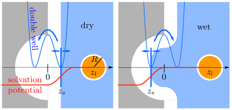
Fig. 1: Illustration of the stochastic model: The interface as pseudo-particle (thick blue ’surface’ line) at position $z_{s}$ fluctuates in the pocket in a double-well potential (eq. (1), blue curve) in $z$-direction leaving the pocket either dehydrated/dry (left) or hydrated/wet (right). The ligand (orange circle) at position $z_{l}$ diffuses freely in one-dimension on the $z$-axis perpendicular to the pocketed wall. It interacts with the interface by an attractive interaction potential (eq. (3), red line). As illustrated here the interaction potential moves with interface. Note the model is spatially purely one-dimensional and the schematics of the pocketed wall (gray) and bulk water area (blue) are just shown for illustration.

The ligand diffuses with the properties of a spherical particle in water utilizing the Einstein relation $D=k_{\rm B}T/6\pi\eta R$, where $k_{\rm B}$ is the Boltzmann constant, $\eta$ the viscosity of the solvent and $T$ the temperature. Dynamic coupling may occur when interface fluctuations and ligand kinetics are on a similar time scale. Hence, simply choosing equal diffusivity for both ligand and pseudo-particles facilitates the condition having both time scales with comparable magnitude. In our model the energy scale $\mathrm{k_{B}T}$ and the length scale $R$ are set to one in the following, as well as the diffusion constant $D$. This introduces a Brownian length scale $\lambda_{B}=R$ and time scale $\tau_{B}=\lambda_{B}^{2}/D$. A detailed comment on the relation of units and physical constants to the previous explicit-water MD simulations is provided in the Appendix A.

As motivated from previous MD studies, we assume that the interface fluctuates bimodally between positions inside or outside the pocket. This models enhanced fluctuations of the water interface penetrating into the pocket. Thus the interface moves as a Brownian pseudo-particle in an external double-well potential

$$V_{dw}(z_{s})=\frac{h}{\lambda_{B}^{4}}\left(z_{s}^{2}-\lambda_{B}^{2}\right)^{2}+b\cdot z_{s}$$ (1)

which is drawn as blue curve in Fig. 1. For $b=0$, the positions of the two wells are situated at $\pm\lambda_{B}$, and $h$, in our energy units, is the height of the barrier which lies at $z=0$. To further enable changes in relative depths of ’dry’ and ’wet’ wells we introduce a bias given by the linearity constant $b$ in $\mathrm{k_{B}T}/\lambda_{B}$.

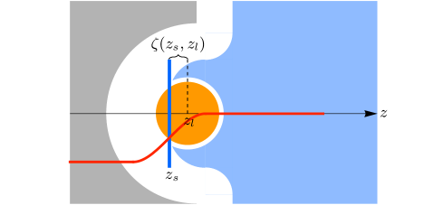
Fig. 2: If the distance $\zeta(z_{s},z_{l})=z_{l}-z_{s}$ fulfills $\Theta(R-|\zeta|)=1$ the water-vapor interface (vertical blue line) and the ligand (orange sphere) interact by the solvation potential (eq. (3), red curve). The interaction scales by the solvated volume of the ligand, which is the portion on the right hand side of the interface.

A pair potential acting between the interface and the ligand accounts for energetic contribution of solvation as the ligand passes through the water interface (see Fig. 2). The resulting solvation potential is designed such that it pushes the ligand out of the solvent into the pocket ($z_{l}<0$). At the same time, following the principle of action-reaction, the interaction pulls the interfacial water out of the pocket ($z_{s}>0$), which conceptually corresponds to ligand-induced drying transition. For small solutes solvation energy approximately scales linearly with solvent excluded volume $\Delta G\propto V$, whereas after the transition at a crossover length-scale $l_{c}$ it is proportional to solvent accessible surface area $A$, $\Delta G=\gamma\cdot A$ with $\gamma$ as surface tension Chandler:Nature . Modeling microscopic key-lock binding with a small-sized ligand, we choose the solvation potential to scale linearly with solute volume, or solvent excluded volume. We demand a reasonable proportionality constant $\Gamma$ to fulfill $\Delta G(l_{c})=\Gamma\cdot V(l_{c})\equiv\gamma\cdot A(l_{c})$ at the crossover length-scale, which thus yields

$$\Gamma=3\gamma/l_{c}\,.$$ (2)

For pure water surface tension we calculate $\Gamma=2.95~{}\mathrm{k_{B}T}/\lambda_{B}^{3}$ (see Appendix A) such that the effective solvation energy is roughly $12.36~{}\mathrm{k_{B}T}$, which is comparable to the results of explicit water simulations Setny:JCTC:2010 . Solvent excluded volume changes with ligand distance to the water interface, $\zeta(z_{s},z_{l})=z_{l}-z_{s}$, as it is illustrated in Fig. 2. The solvation potential is then written as

$$\Delta G(z_{s},z_{l})=\Gamma\left[\frac{4\pi}{3}R^{3}-\frac{\pi}{3}(R-\zeta)^{2}(2R+\zeta)\right]$$ (3)

which gives a parabolic pair force, acting on particle $x=s,l$ (solvent or ligand)

$$F_{sol}^{x}(z_{s},z_{l})=-\frac{\mathrm{d}\Delta G(\zeta)}{\mathrm{d}\,\zeta}\frac{\mathrm{d}\zeta}{\mathrm{d}z_{x}}=\pi\Gamma(\zeta^{2}-R^{2})\frac{\mathrm{d}\zeta}{\mathrm{d}z_{x}}$$ (4)

The solvation potential only acts when the separation of the ligand to the interface is smaller than $R$ which can be expressed by the Heaviside step function $\Theta(R-|\zeta|)$. For clarity, however, it is omitted in eq. (3) and (4).

The gray wall in Fig. 1 embedding the cavity is only drawn representatively. Naturally the system describes the bimodal water interface fluctuations due to hydrophobic confinement, but a potential incorporating steric repulsion and van der Waals attraction is omitted. It is not needed here since numerical simulation of unrestrained ligand motion is aborted every time the ligand is bound, namely when $z_{l}=-1.25$.

Also, we fix a reflective boundary to a given distance $z_{max}$ to the pocket in order to avoid the ligand diffusing far away from the pocket. Throughout the main body of the paper $z_{max}=5$, whereas in Appendix C the impact of the choice of $z_{max}$ is discussed.

In summary, two nonlinearly coupled Langevin equations describe the key-lock system by

$$\xi_{s}\dot{z}_{s}(t) =+\pi\Gamma\left(R^{2}-\zeta(z_{s},z_{l})^{2}\right)\cdot\Theta\left[R-|\zeta(z_{s},z_{l})|\right]-4\frac{h}{\lambda_{B}^{4}}z_{s}(z_{s}^{2}-\lambda_{B}^{2})-b+F_{s}(t)$$ (5a)

$$\xi_{l}\dot{z}_{l}(t) =-\pi\Gamma\left(R^{2}-\zeta(z_{s},z_{l})^{2}\right)\cdot\Theta\left[R-|\zeta(z_{s},z_{l})|\right]+F_{l}(t)$$ (5b)

with $\xi_{x}$ as friction coefficients, $x=s,l$, and $F_{x}(t)$ denoting $\delta$-correlated random forces fulfilling fluctuation-dissipation theorem $\langle F_{x}(t)F_{x}(t_{0})\rangle=2\mathrm{k_{B}T}\xi_{x}\delta(t-t_{0})$. Note that both $\xi_{s}=\xi_{l}=1$ since here diffusivities of both ligand and pseudo-particle interface are set equal.

III Numerical simulations

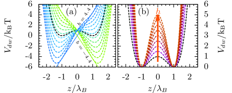
Fig. 3: The double-well potential which governs solvation fluctuations in the pocket: The fluctuations are tuned by (a) biasing from $b=-4.4~{}\mathrm{k_{B}T}/\lambda_{B}$ to $4.4~{}\mathrm{k_{B}T}/\lambda_{B}$ in steps of $0.8~{}\mathrm{k_{B}T}/\lambda_{B}$, hence breaking rate symmetry, or (b) barrier height from $h=1~{}\mathrm{k_{B}T}$ to $5\,\mathrm{k_{B}T}$ in steps of $0.5~{}\mathrm{k_{B}T}$, thus changing the magnitude of the interface’s characteristic time scales. Black dashed lines draw the reference double well setting ($h=1$, $b=0$). Example biasing $b$ or changes in magnitude $h$ are indicated by example guide lines (a) or arrow (b), respectively. (Color coding is maintained throughout the paper.)

In the following we discuss binding kinetics obtained from integrating the equations (5) numerically, where we use the numeric scheme proposed by Ermak and McCammon Ermak&McCammon . We focus on how their coupling affects the ligand’s reaction coordinate $z_{l}(t)$ kinetics, and how changes in the interface dynamics impact. In general, pocket solvation can be affected by changing its hydrophobicity, geometry or size. Such changes, however, simultaneously affect pocket occupancy and solvent fluctuation time scale. In our model, we have the ability to disentangle both effects and their influence on ligand binding.

Water occupancy can be tuned by changes in the biasing parameter $b$ of the double well potential, $V_{dw}$. Potentials with biasing ranging from $b=-4.4\,\mathrm{k_{B}T}/\lambda_{B}$ to $b=4.4\,\mathrm{k_{B}T}/\lambda_{B}$ in steps of $0.4\,\mathrm{k_{B}T}/\lambda_{B}$ are drawn in Fig. 3 (a). The black dashed line refers to the reference with barrier height $h=1\,\mathrm{k_{B}T}$ and no biasing, which is motivated from explicit and implicit solvent simulation studies Setny:PNAS ; Setny:PRL . The barrier height can separately be tuned from $h=1\,\mathrm{k_{B}T}$ to $h=5\,\mathrm{k_{B}T}$ in steps of $0.5\,\mathrm{k_{B}T}$ as plotted in Fig. 3 (b). Changes in barrier height directly influence the wet-dry transition time and thus the effective interface fluctuation time scale. From Kramer’s rate theory one knows that the rate $r$ of crossing the double well barrier scales exponentially with barrier height $r\propto\mathrm{e}^{-h}$ Hänggi:KramersReview . The color coding from both plots in Fig. 3 is consistently adopted to other plots throughout this paper.

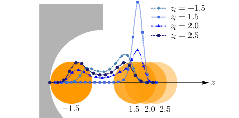
Fig. 4: The equilibrium distribution (blue lines) of the water interface is affected by the ligand position due to the hydrophobic ligand-interface interaction in eq. (3) and (4). As the ligand (orange circle) approaches the pocket, the bimodality of the water interface distribution is lost for intermediate states, e.g. $z_{l}=1.5$, but is recovered if the ligand is fully bound to the pocket, e.g., $z_{l}=-1.5$.

Further we note that the equilibrium distribution of the water interface depends on the ligand position due to the nonlinear coupling evident from contributions of eq. (4) in (5) if $|\zeta|<R$. A schematic plot in Fig. 4 illustrates how the bimodal distribution changes while the ligand comes closer to the pocket. When the ligand and the interface interact, their pair potential adds to the effective equilibrium free energy landscape of the pseudo-particle. This can tilt the bimodal distribution of the interface and thus influences the equilibrium wetting behavior of the pocket. We observe that the pocket drying is enhanced for close ligand positions which coarsely mimics also how pocket hydration couples to ligand position in all-atom and implicit solvent simulations Setny:PRL ; Setny:PNAS .

III.1 Mean first passage time and memory

As first measure of ligand binding kinetics the mean first passage time (MFPT) is sampled from each point $z$ to a bound configuration at $z_{f}=-1.25$. Therefor, for each setup with given biasing $b$ and barrier height $h$ around $2\times 10^{5}$ trajectories are simulated and analyzed for the ligand starting at $z_{max}=5$ until it is $<1.25$ inside the pocket. Hence, the resulting MFPT curves describe the mean first passage time $T_{1}(z,z_{f})$ of the ligand crossing $z_{f}=-1.25$, given it started at $z$ with a reflective boundary at $z_{max}=5$.

Fig. 5 (a.1) shows the MFPT curves corresponding to simulation setups with varying bias in the double-well potential the interface coordinate is subject to. Starting with setups with a negative bias (greenish lines), hence a preferentially dry pocket, the ligand’s mean binding time is faster than without biasing (black). With growing values for the bias the MFPT slows down by a factor of two. Also, as the barrier height increases, a deceleration of the MFPT is observed in Fig. 5 (b.1). There the MFPT curves exhibit a hunch around $z\approx 1$ which is enhanced with growing barrier whereas at $z=0$ all curves $T_{1}(z,z_{f})$ in panel (b.1) coincide.

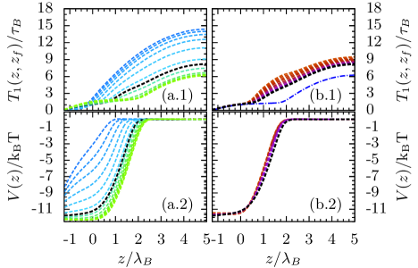
Fig. 5: MFPT curves $T_{1}(z)$ and PMF $V(z)$ of ligand binding to the pocket depend on changes of interface’s fluctuation behavior by double-well variations from Fig. 3. Panel (a.1)/(a.2) shows ligand’s MFPT/PMF dependent on double-well biasing $b$. Panel (b.1)/(b.2) draws ligand’s MFPT/PMF dependent on double-well barrier height $h$. Blue dash-dotted line in panel (b.1) draws an example MFPT curve $T_{1}^{\mathrm{M}}(z)$ using eq. (6) for the reference setting ($h=1$, no bias) with respective PMF and constant diffusivity. (Color coding is adopted from Fig. 3.)

Further, we analyze for all considered parameter values $(h,b)$ the potential of mean force (PMF) of the ligand using the weighted histogram analysis method (WHAM) Ferrenberg&Swendsen ; Kumar&Rosenberg ; Zhu&Hummer along $z$. Fig. 5 (a.2) shows a strong dependence of the PMFs on the biasing parameter $b$. Besides small changes in shape, the attractive part of the PMFs essentially shifts towards smaller values of $z$, if the interface bias shifts towards an increasingly wetted pocket. On the other hand, the ligand PMF negligibly depends on the barrier height, $h$, as revealed in Fig. 5 (b.2). The PMF, as an equilibrium quantity, is essentially unaffected since mainly interface kinetics change with $h$. This is especially noteworthy since the corresponding MFPT curves in panel (b.1) alter relatively strongly with $h$, suggesting that the effect on ligand binding times originates from modified interface kinetics.

In the case of a Markovian process the PMF, $V(z)$, together with possibly spatially dependent diffusivity, $D(z)$, determine the $n$-th moment of the first passage time distribution Siegert ; Weiss

$$T_{n}^{\mathrm{M}}(z,z_{f})=n\int\limits_{z_{f}}^{z}\mathrm{d}z^{\prime}\frac{\mathrm{e}^{V(z^{\prime})}}{D(z^{\prime})}\int\limits_{z^{\prime}}^{z_{max}}\mathrm{d}z^{\prime\prime}\mathrm{e}^{-V(z^{\prime\prime})}\cdot T_{n-1}^{\mathrm{M}}.$$ (6)

where the zeroth moment $T_{0}^{\mathrm{M}}=1$ determines normalization. Note that $\beta=\mathrm{k_{B}T}^{-1}=1$ is omitted in the Boltzmann factors in the above equation as it will be in later occurrences. The blue, dash-dotted line in Fig. 5 (b.1) is a numerically integrated solution of equation (6) using constant diffusivity $D(z)=1$, and spatially dependent $V(z)$ of the reference case $b=0$ and $h=1$. It should be compared to the black, dashed MFPT curve in the same plot. Only for negative $z$-values both coincide. Effects that can no longer be treated by Markovian kinetics occur around $z\approx 1$, where the hunch in simulated MFPT curves qualitatively deviates to a dent in the solution of equation (6). For even bigger values of the reaction coordinate, shapes of the MFPT curves of both methods only conform, but the Markovian solution represents overall faster association. Together the ligand dynamics only can be modeled by pure Markovian description when the ligand is inside the pocket.

As a general measure, calculating MFPT curves $T_{1}^{\mathrm{M}}$ in a Markovian picture for all considered cases of bias strengths and barrier heights, and using the respective PMFs, enables direct observations where the deviations in simulation occur. Accordingly, the difference $T_{1}(z,z_{f})-T_{1}^{\mathrm{M}}(z,z_{f})$ is plotted in Fig. 6 (a.1) and (b.1). In all cases the difference vanishes inside the pocket and increases towards a maximum situated just in front of the pocket mouth. It then plateaus to a constant positive value for large $z$, which indicates slowed ligand kinetics in all considered cases of pocket water fluctuations. For the cases of biased wetting, the difference $T_{1}-T_{1}^{\mathrm{M}}$ in Fig. 6 (a.1) is very small, if the pocket is preferably dry, namely with a strong negative bias. As the biasing parameter $b$ increases, and thus the interface’s distribution tends towards mainly hydrated pocket states, the difference in MFPT accumulates to a peak when $b=2.8\mathrm{k_{B}T}/\lambda_{B}$, and alleviates for even higher bias. In Fig. 6 (b.1) deviations to the Markovian picture are enhanced by growing barrier height, hence slowed-down wetting fluctuations.

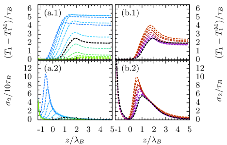
Fig. 6: Markovian assumption breaks down as manifested in differences of MFPT $T_{1}(z)$ from simulation to $T_{1}^{\mathrm{M}}(z)$ from eq. (6) and in memory index $\sigma_{2}(z)$ from eq. (7). Panels (a.1) and (a.2) show the respective measures dependent on the double well bias $b$. Panels (b.1) and (b.2) draw both measures dependent on double well barrier height $h$. Note that the effect is much bigger as the biasing towards a wet pocket increases. Therefore the scale of (a.2) is $\sigma_{2}/10\tau_{B}$. (Color coding is adopted from Fig. 3.)

In order to investigate further the break-down of Markovian dynamics and possibly accompanied memory, we additionally determine the, so called, memory index Hänggi&Talkner

$$\sigma_{2}=\frac{T_{2}(z,z_{f})-T_{2}^{\mathrm{M}}(z,z_{f})}{T_{1}(z,z_{f})}$$ (7)

introduced by Hänggi et al. Hänggi&Talkner who noted its possible value to ligand migration studies. It provides an additional spatially resolved measure of the character of a random process. It indicates a process to be non-Markovian if the difference of the second moment of a random process to the second moment of the corresponding process with Markovian assumption does not vanish. For all considered cases of pocket wetting behavior Fig. 6 (a.2) and (b.2) show that $\sigma_{2}$ vanish for ligand positions far from the pocket. Note, however, that finite $\sigma_{2}$ values are reached already at intermediate positions, that is $z\sim 3$, where the ligand is still out of reach of the solvation potential ($\zeta(z_{l},z_{s})>R$). Finally, the memory index peaks at the position $z\lesssim 1$, at which initial deviations in the first moments occur in Fig.6 (a.1) and (b.1). Subsequently, for $z<1$, it steeply recedes to zero. Inside the pocket $\sigma_{2}$ diverges once more, majorly due to numerical inaccuracies close to the target distance as these are amplified by division in eq. (7). Also, actual non-Markovian effects reoccur inside the pocket as it becomes evident from results and discussions in following sections and in Appendix B.

All together it is inept to assume constant ligand diffusivity within a Markovian description of our ligand-interface system in order to estimate correct mean binding time. The process rather indicates non-Markovian contributions, slowing the ligand binding which predominantly arise in the region where the ligand and the interface start interacting. Overall, the first and second moments are influenced far outside where the ligand is driven by delta correlated random noise by definition in eq. (5). In addition, strongly dissimilar MFPTs but almost similar PMFs in Fig. 5 (b.1) and (b.2), respectively, suggest that local coupling of interface time scales alone is enough to impact ligand binding kinetics.

III.2 Spatially dependent friction

In order to illuminate the kinetic effect we restrict further analysis to systems considering an unbiased interface distribution, but varying only the barrier height $h$ in the double-well potential. For these particular cases, a purely kinetic nature of the observed effects was evident from the perturbation of average ligand binding times occurring with unchanged PMF, as shown in Fig. 5.b.

Spatially resolved friction $\xi_{l}(z)$ can be obtained from the position auto-correlation function (PACF), $\langle\delta z_{l}(t)\delta z_{l}(0)\rangle_{r}$, with $\delta z_{l}(t)=z_{l}(t)-z_{r}$, derived from simulations with the ligand harmonically restrained at $z_{r}$. A detailed description of ligand umbrella simulation is provided in Appendix B. Integration of the auto-correlation function provides the time scale which is divided by the square of the position fluctuations, yielding the local friction Hummer

$$\xi(z_{r})=\frac{\int_{0}^{\infty}\langle\delta z_{l}(t)\delta z_{l}(0)\rangle_{r}\mathrm{d}t}{\langle\delta z_{l}^{2}\rangle_{r}^{2}}\,\,\,.$$ (8)

Solid curves in Fig. 7 (c) show Gaussian fits to $\xi(z_{r})$, gathered from PACF evaluation (see also Appendix B). Simulations restraining the ligand far away from the pocket yield the preset friction of value one. However, $\xi(z)$ strongly peaks in front of the pocket mouth, where the ligand is subject to interaction with the interface. Growing barrier height, and thus exponentially slowed double-well transition rates of the interfacial motion, increases the peak up to a factor of approximately 85. It indicates that the effect arises due to the ligand interacting with the bimodally fluctuating interface. While the interface penetrates the pocket, the ligand, still remaining around $z\sim 2.0$, is only subject to the $\delta$-correlated random force of the Langevin model eq. (5). Whereas when the interface is in the outer well in front of the pocket, the solvation potential acts on the ligand. Hence the solvation force acts as additional fluctuating force which introduces additional friction. Peaking friction occurs in regions in which fluctuations are most pronounced, where interface and ligand might interact or not, and thus the solvation potential can essentially be on or off.

Together with the observations throughout previous MFPT analysis it seems that the additional force fluctuations serve as a source of memory. Their time scale is proportional to the Brownian time, $\tau_{B}$, and scales exponentially with double well barrier height: $\tau_{dw}\propto\tau_{B}\mathrm{e}^{h}$ (see also eq.(17)). Thus the time scale of the solvation force fluctuations does not separate from the time scale of ligand migration, which leaves memory to the association process. As it will be shown in the following section a generalized Langevin model derives an exponential growth of the friction peak values with barrier height, which directly relates to exponentially growing time scales of the interface fluctuations.

Again we obtain the MFPT curve $T_{1}^{\mathrm{M}}(z,z_{f})$ using equation (6), with the PMF $V(z)$ of the reference case $(h=1,b=0)$, and now additionally with a spatially resolved diffusion $D(z)~{}=~{}\mathrm{k_{B}T}~{}\cdot~{}\xi^{-1}(z)$ from Einstein’s relation, with previously evaluated $\xi(z)$. Only in the interval $z\in(-1.25,0.5)$ the result, plotted as green dash dotted line in Fig. 7 (a), coincides with MFPT curves from simulation (black dashed), and moreover, with evaluation of eq. (6) without spatially resolved friction (blue dash dotted). Subsequently, a steep edge in the curve yields values which overestimate the actually simulated results far outside, $z\gg 2$. So, on one hand, the solution of equation (6) overestimates the results using both spatially resolved profiles $V(z)$ and $\xi(z)$. On the other hand, it is underestimated using only spatially resolved PMF, but constant friction of value one.

For comparison we also calculate spatially dependent profiles $\xi^{\mathrm{M}}(z)=\mathrm{k_{B}T}/~{}D^{\mathrm{M}}(z)$ by solving equation (6) for $D(z)\equiv D^{\mathrm{M}}(z)$ as primarily introduced by Hinczewski et al. Hinczewski&Netz

$$D^{\mathrm{M}}(z)=\frac{\mathrm{e}^{V(z)}}{\partial T_{1}(z)/\partial z}\int_{z}^{z_{\mathrm{max}}}\,\mathrm{d}z^{\prime}\,\mathrm{e}^{-V(z^{\prime})}.$$ (9)

Note that $\xi^{\mathrm{M}}(z)$ uses the Markovian assumption, and thus, is certainly not the proper friction profile fulfilling fluctuation-dissipation theorem for our non-Markovian ligand migration process. In detail, it does not measure the quantity friction/dissipation which can be proportionally related to the system’s fluctuations. However, it will trivially reproduce the correct MFPT $T_{1}$ from simulation when using it in eq.(6). Dashed lines in Fig. 7 (c) show curves for $\xi^{\mathrm{M}}(z)$ which similarly peak in front of the pocket mouth. In exact comparison to $\xi(z)$ from PACF, the results from eq. (9) show a positional shift closer to the pocket and differ in peaking value as well as peak width. (Additional information on how $\xi^{\mathrm{M}}(z)$ depends on the choice of reflective boundary is discussed in the Appendix C.)

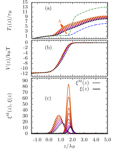
Fig. 7: Panel (a) draws again the MFPT curves from simulation already shown in Fig. 5 (b.1). Here it also compares to a MFPT curve $T_{1}^{M}(z)$ for the reference setting calculated from eq. (6) with PMF and spatially dependent friction from PACF plotted as green dash-dotted line. Panel (b) draws again the PMFs already shown in Fig. 5 (b.2). Panel (c) plots spatially resolved friction $\xi(z)$ from fits to PACF data eq. (8) (solid) and from MFPT data using eq. (9) with Einstein relation $\xi^{\mathrm{M}}(z)=k_{B}T/D^{\mathrm{M}}(z)$ (dashed). (Color coding is adopted from Fig. 3.)

Again, observing essential discrepancy between local friction $\xi(z)$ from simulation and a spatial profile $\xi^{\mathrm{M}}(z)$ from a memoryless picture in eq. (9) illustrates the location and strength of non-Markovian effects within the Langevin system (5). Also, whether calculating MFPTs from eq. (6) either with constant friction or spatially resolved friction $\xi(z)$, yields under- and overestimated results, respectively. In neither case the Markovian property is fulfilled, which is the requirement for obtaining a proper system description with eq. (6). We emphasize that our system exhibits similar non-Markovian effects as those resolved by explicit water simulations from Setny et al. Setny:PNAS .

IV Generalized Langevin model

Having identified fluctuations of the solvation potential as the origin of local memory and friction in the ligand’s reaction coordinate we show in the following how their impact can be quantified. Further, this section shall formulate the proper stochastic characteristics when dealing with the ligand coordinate alone. For simplicity it focuses on local conditions, namely, constrained ligand position. Yet it elucidates a proper non-Markovian formulation to classify possible treatment with conventional theory.

Generally in the case of a known memory kernel $\eta(t)$ one can directly investigate the corresponding one-dimensional general Langevin equation (GLE)

$$m\ddot{q}(t)=-\frac{\partial V_{eq}(q)}{\partial q}-\int^{t}\mathrm{d}t^{\prime}\eta(t-t^{\prime})\dot{q}(t^{\prime})+\mathcal{F}(t)$$ (10)

with mass $m$, equilibrium potential $V_{eq}(q)$, and a random force fulfilling fluctuation dissipation $\langle\mathcal{F}(t)\mathcal{F}(t^{\prime})\rangle=2\mathrm{k_{B}T}\eta(t-t^{\prime})$. Simple systems of two coupled Langevin equations can be analytically contracted onto a one-dimensional GLE Risken ; vanKampen and vice versa. A prominent example is that of an underdamped Brownian particle in a harmonic potential. For the coupled system described by eq. (5) analytic contraction from 2D to 1D is not feasible due to higher than harmonic coupling and nonlinearity in the double-well potential. Therefor we reinterpret a method which is usually used to expand a one-dimensional GLE to a set of two coupled equations without memory. With that we are able to approximate friction from local conditions of the pocket-ligand system. We restrict the analysis to the location of the friction peaks discussed above and can predict the peaking value $\mathrm{max}(\xi(z))$ as function of barrier height in a bimodally fluctuating force.

To this end we reverse the approach from Pollak et al. Risken ; Pollak&Berezhkovsii ; Berezhkovsii&Pollak . It originally extends a one-dimensional GLE of reaction coordinate $q$ such as eq (10) by an auxiliary variable $x$ to receive two coupled equations. Each of the resulting equations then omits memory and only the auxiliary variable $x$ is driven by a temporally delta correlated random force, $N(t)$. Taking unit mass $m=1$, the GLE (10) is mapped on the two dimensional, underdamped system

$$\ddot{q}+\frac{\partial V(q,x)}{\partial q} =0$$ (11a)

$$\xi\dot{x}+\frac{\partial V(q,x)}{\partial x} =N(t).$$ (11b)

The driving noise $N(t)$ is a delta correlated Gaussian noise

$$\langle N(t)\rangle=0,\,\,\,\,\langle N(t)N(t^{\prime})\rangle=2\mathrm{k_{B}T}\xi~{}\delta(t-t^{\prime})\,.$$ (12)

There are two further requirements that memory $\eta(t)$ and coupling potential $V(q,x)$ must fulfill for proper mapping Pollak&Berezhkovsii ; Berezhkovsii&Pollak :

1. The kernel $\eta(t)$ may be represented by a sum of exponentials, and for this very example even

   $$\eta(t)=\frac{\xi}{\tau}\mathrm{e}^{-t/\tau}\equiv\Omega\mathrm{e}^{-t/\tau}.$$ (13)

2. The coupling between auxiliary and reaction coordinate should be harmonic such that

   $$\frac{\partial V(q,x)}{\partial q}=\frac{\mathrm{d}V_{eq}(q)}{\mathrm{d}q}-\Omega[x-f(q)]\frac{\mathrm{d}f(q)}{\mathrm{d}q}.$$ (14)

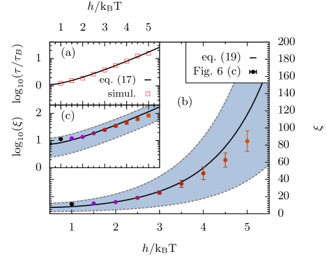
Fig. 8: Panel (a) plots time scale $\tau_{dw}(h)$ of the interfacial motion in the double-well without ligand. Black line refers to eq. 17 and orange squares are values obtained by interface’s position auto-correlation from simulation. Panel (b) shows $\xi(h)$ (eq. (19)) from constructed GLE using $\epsilon=0.36$ (black line) and blueish shaded area delimited by gray dashed lines indicates the range covered by eq. 19 with standard deviation $\Delta\epsilon=\pm 0.24$. The peaking values from $\xi(z)$ in Fig. 7 (c) are here shown as circular symbols with corresponding color coding from Fig. 7. Panel (c) plots the same data as in (b) on a log-scale.

In our case, let us focus on the situation at the position of the friction peak, $\mathrm{max}(\xi(z))$ in Fig. 7 (c). In that case the expansion $\mathcal{T}_{1}^{\epsilon}$ of the solvation force in eq. (4) at fixed ligand-interface distance $\epsilon$ up to first order, with respect to a perturbation $\delta\zeta=\zeta-\epsilon$, gives the harmonic contribution of our solvation coupling

$$\mathcal{T}_{1}^{\epsilon}~{}F_{sol}(\zeta)=\pi\Gamma[\epsilon^{2}-R^{2}]+2\pi\Gamma\epsilon(\zeta-\epsilon)+\mathcal{O}(\zeta^{2})$$ (15)

which identifies the memory kernel constant, $\Omega=\xi/\tau=2\pi\Gamma\epsilon$, by comparison with eq. (14). The value of $\epsilon\approx 0.36\pm 0.24$ is estimated from simulations constraining the ligand at the position of the friction peaks in Fig. 7. It is the mean and standard deviation of the distribution of distance $\zeta$ between constrained ligand and bimodally fluctuating interface. Detailed evaluations of $\epsilon$ are discussed in Appendix D. The set of coupled equations of motion of a free ligand (here $q_{l}$) coupled to an auxiliary variable $x_{s}$ are adopted to the requirements (a) and (b) described above such that

$$\ddot{q}_{l}-2\pi\Gamma\epsilon(q_{l}-x_{s}-R) =0$$ (16a)

$$\xi\dot{x}_{s}+2\pi\Gamma\epsilon(q_{l}-x_{s}-R) =N(t).$$ (16b)

Note that the system of the two above equations is not equivalent to the original coupled Langevin system (5). With the aim to formulate the influence of interface fluctuations on local friction encountered by the ligand, it describes only a single system configuration, which determines the $\epsilon$.

A striking difference is that eq. (16) does not implement the double-well itself. Rather the time scale determining the memory is chosen to be that of a Brownian particle in a double-well. A compact approximate solution of that time scale is given by Cregg&Wickstead ; Kalmykov&Waldron

$$\tau_{dw}(h)=\frac{\tau_{B}}{2\sqrt{2h}}\frac{(\mathrm{e}^{h}-1)}{2h}(\pi\sqrt{h}+2^{1-\sqrt{h}})\,\,\,.$$ (17)

To confirm the approximation for the setups we previously considered, we probe the time scale of interface fluctuations in the double-well within simulations without ligand. Tuning the barrier height from $h=1~{}\mathrm{k_{B}T}$ to $h=5~{}\mathrm{k_{B}T}$ reveals that the approximate formula (17) is in very good agreement within the range of interest in $h$ (Fig. 8 (a)).

The GLE corresponding to (16) with memory from (17) is followingly given by

$$\ddot{q}_{l}(t)=-2\pi\Gamma\epsilon\int^{t}\mathrm{d}t^{\prime}~{}\mathrm{e}^{-(t^{\prime}/\tau_{dw})}\dot{q}_{l}(t^{\prime})+\mathcal{F}(t)\,\,\,.$$ (18)

Comparison of its memory kernel with eq. (13) determines the friction for the constructed system such that

$$\xi(h)=\Omega\cdot\tau=2\pi\Gamma\epsilon\cdot\tau_{\text{dw}}(h)\,.$$ (19)

Fig. 8 (b) and (c) demonstrate the strong resemblance of both systems, the fully coupled key-lock binding model (5) and the non-Markovian model (18). The circular symbols with error bars from Gaussian fits draw the maxima of the friction peaks $\mathrm{max}(\xi(z))$ (from Fig. 7) from PACF calculations of the original key-lock model (5). The black line draws expression (19) found for $\xi(h)$. The blue shade indicates the error from variance calculations to $\epsilon$.

V Concluding Remarks

Our investigations presented here reveal the origin of increased friction and additional memory in hydrophobic pocket-ligand binding as it was observed in previous work using all-atom simulations Setny:PNAS ; Mondal:PNAS . We employ a simple stochastic model of two nonlinearly coupled Langevin equations each driven with memoryless Gaussian noise. One equation models pocket hydration in terms of a continuously diffusing pseudo-particle as an interface, which can occupy the pocket volume or sample the region in front of the pocket entrance. Another one describes a ligand, freely diffusing on an effectively one-dimensional reaction-coordinate, which is subject to solvation force when in contact with the interface. Thus, a nonlinear coupling is an effective interaction potential between the pseudo particle and the ligand, motivated from solvation free energy of a microscopic hydrophobic ligand scaling with the solvated volume. The model enables investigation on tunable interface motion, hence pocket hydration, by biasing a double well potential which leaves the pocket in rather ’wet’ or rather ’dry’ states, as well as by changing its barrier height, thus affecting the respective transition rate. Incorporating the double-well behavior of pocket hydration was essentially motivated from the bimodal water occupancy distributions observed in hydrophobic confinement by Setny et al. Setny:PNAS .

Even though the system was driven by simple Markovian delta-correlated random forces, the first passage time analysis of ligand binding revealed non-Markovian contributions to binding kinetics. In all cases of bimodal water interface fluctuations, ligand association kinetics from numerical simulation of the model was decelerated in comparison to a Markovian picture, utilizing equilibrium PMF and spatially constant friction. Deviations of numerical simulations from the Markovian description were spatially resolved for comparison of the first and the second moments of the first passage times of binding to the pocket. Comparison of the moments indicated non-Markovian contributions to occur shortly before binding, at positions where the ligand is subject to intermittent interaction with the bimodally fluctuating interface. Otherwise the Markovian behavior is restored if the ligand is already inside the pocket, where the pair potential inhibits bimodal interface fluctuations and leaves the pocket in a rather dry state.

Especially when hydration fluctuation time scales were changed by tuning double-well barrier height, the ligand PMFs basically remained unchanged. At the same time, the deceleration of ligand binding was enhanced by increasing interface relaxation times. Together it raised evidence that ligand kinetics couples to the time scale of water fluctuations due to the fluctuating potential, which in all-atom simulations refers to a fluctuating PMF Mondal:PNAS .

We resolved friction of the ligand by position auto-correlation and found spatially dependent friction in front of the pocket. It was found to peak at positions where coupling to the water interface occurs time-dependently. As the ligand is situated at the edge of the interface’s external double-well it is subject to the solvation potential only for given time periods. The situation exhibits a bimodally on-off switching of coupling and thus facilitates additional force fluctuations, yielding additional friction.

We corroborate the origin of memory by constructing a generalized Langevin model restricted to local conditions of the original two coupled Langevin equations. It utilized the interaction potential between the ligand and the interface, as well as the auto-correlation time of the interface fluctuation as time scale of the memory kernel. The derived friction and noise strength of the GLE (18) was shown to coincide with the observed modulations in spatial ligand friction from simulations of eq. (5).

In general, additional friction and memory in hydrophobic key-lock binding can originate from coupling of water fluctuations to the ligand diffusion when both occur on comparable time scales, as shown here and in previous MD studies Setny:PNAS ; Mondal:PNAS . Essentially, the pocket water fluctuations behave as strong and comparably slow fluctuations of the mean forces (PMF) to the ligand. Within the course of this paper especially bimodal fluctuations of the coupling facilitate strong on-off force fluctuations. These do not rank as the fast solvent molecular forces for which ligand and solvent time scales separate which can be coarse-grained in a random force kernel delta-correlated in time. Instead, the slow solvent fluctuations in the pocket rather add to ligand friction including memory as fluctuation-dissipation theorem predicts, dissipative forces (friction) to be proportionally related to a system’s intrinsic fluctuations.

With this the paper illustrated the kinetic characteristics of ligand association coupling to pocket water occupancy fluctuations. It suggests to future studies on ligand-receptor systems to apply elements of conventional kinetic theory which also accounts for situations when time scales do not separate. For extreme cases with bimodal wetting fluctuations, a two-state approach has been successfully applied in ref. Mondal:PNAS , suggesting possible consideration in reaction-diffusion models, multistate models Zhou ; Szabo:JCP or even Markov-state models Bowman&Noe ; Hummer&Szabo . Other studies Mondal:JCTC make evident that ligand binding is not necessarily accompanied by bimodal pocket occupancy fluctuations. If, in such cases, memory remains corrections to a Kramer’s rate of ligand binding and unbinding, can be determined within Grote-Hynes theory Grote&Hynes and generalizations of it Hänggi . Beyond known kinetic approaches to ligand-receptor binding it remains to future work to investigate fundamental and worthwhile treatment considering position dependent memory as a ligand’s position influences the (water) fluctuations it couples to.

Appendix A Units and constants

The Langevin system in eq. (5) is strongly inspired by the all-atom simulation setup in ref Setny:PNAS . Therefore all units are directly related to the system of the corresponding MD setup. Those were conducted in ambient conditions which is why effective temperature during the numerical simulations of eq. (5) relates to $T=300$ K. The particle size of the ligand is that of a methane molecule which is roughly $R=0.4$ nm which sets the Brownian length scale $\lambda_{B}$. With viscosity $\eta\approx 10^{-3}\,$Pa$\cdot$s of water Smith:SPCEvisco the corresponding diffusion constant relates to $D=\mathrm{k_{B}T}/6\pi\eta R=0.54\,\mathrm{nm}^{2}\,\mathrm{ns}^{-1}$.

For parametrization of the solvation potential we assume the crossover length-scale at $l_{c}=1$ nm which relates to $l_{c}=2.5\,\lambda_{B}$. With surface tension $\gamma\approx 15.36\,\mathrm{k_{B}T}/\mathrm{nm}^{2}$ for water Vega:SPCEtens we calculate the solvation volume scaling constant $\Gamma=3\gamma/l_{c}=46.1\,\mathrm{k_{B}T}/\mathrm{nm}^{3}=2.95\,\mathrm{k_{B}T}/\lambda_{B}^{3}$.

Appendix B Umbrella sampling simulations

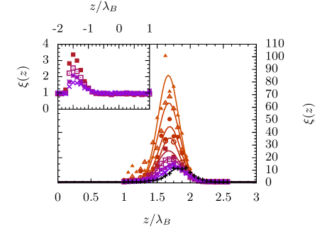
Fig. 9: Symbols represent spatial friction coefficients $\xi(z_{r})$ at restraining positions $z_{r}$. Peaking values increase with increasing double-well barrier height represented in varying color. Gaussian fits of to the respective data are plotted as solid lines. The inset shows similarly peaking frictions when the ligand is inside the pocket and thus randomly interacts with the interface, whereas here $h=(1.5,~{}2,~{}2.5,~{}3)~{}\mathrm{k_{B}T}$. (Color coding is adopted from Fig. 3.)

For a given set of parameters for eq. (5) umbrella sampling simulations were conducted. The simulations implemented harmonic restraining forces $F_{H}=-k(z(t)-z_{r})$ as external force to the ligand with a spring constant of $k=53.92~{}\mathrm{k_{B}T}/\lambda_{B}^{2}$.

For PMF calculation umbrella histograms with a resolution of $0.025$ were generated from $z=-2$ to $z=5.25$ in steps of $0.125$. In house software implementing WHAM was used to determine the unbiased equilibrium distribution from the biased umbrella sampling distribution yielding the PMFs by Boltzmann inversion.

For the purpose of friction calculations $\xi(z_{r})$ by means of PACF umbrella setups were restraining the ligand at positions $z_{r}=1$ to $2.625$ in steps of $0.125$. The choice of the interval was made by an initial coarse scan from positions $z_{r}$ deep inside the pocket up to distances far away. The resulting values $\xi(z_{r})$ were fitted by a Gaussian illustrated in Fig. 9 for simulations utilizing barrier height $h=1~{}\mathrm{k_{B}T}$ to $5~{}\mathrm{k_{B}T}$ in steps of $0.5~{}\mathrm{k_{B}T}$. A second friction peak was also found inside the pocket around $z=-1.5$ as plotted in the inset of Fig. 9. The $h$-dependence is similar because the essential underlying reason is the same but it is not of further relevance to our discussion. A doubled spring constant gave similar $\xi(z_{r})$ within errors of approximately $5\%$ thus confirming sufficient choice of the spring constant.

Also note that sampling has to be increased when barrier height was increased in order to sufficiently sample slowed water fluctuations. Elongated simulations were performed for statistically converged PACF calculation. Still, however, the data remains more noisy for simulations with extended water fluctuation time scales.

Appendix C System size dependence of $\xi^{\mathrm{M}}(z)$

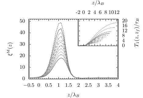
Fig. 10: The peak in $\xi^{\mathrm{M}}(z)$-profiles increase with system size namely when the reflective boundary $z_{max}$ outside the pocket has larger values. The peaking values are proportional to the slope in the MFPT curves, shown in the inset, which increases with $z_{max}$ due to extendedly available trajectories to the random process of ligand migration.

The peak height of $\xi^{\mathrm{M}}(z)$ can easily be shown to be a system size effect from the way the method from Smoluchowski approach is met in eq. (6) and hence eq. (9). The MFPT at each point depends on the choice of reflective boundary $z_{\mathrm{max}}$ because it enters as a boundary to the integral. This becomes most evident when one considers for example a process with constant $V(z)=0$ and constant diffusivity $D$. Equation (6) then simply yields

$$T_{1}(z,z_{f})=-1/2D~{}(z^{2}-z_{f}^{2})+z_{\mathrm{max}}(z-z_{f})\,.$$ (20)

Thus, the MFPT at each position $z$ increases with $z_{\mathrm{max}}$ contributing to an increase in the slope of the curve that enters eq. (9).

Certainly it can also be observed from simulations of our Langevin equations (5). Using the Markovian approach to extract the profiles $\xi^{\mathrm{M}}(z)$ from PMFs and MFPT curves utilizing eq. (9) is also system size dependent. The initial expression for $T_{1}(z,z_{f})$ eq. (8) assumes a diffusion process between a perfect reflective and absorbing boundary Siegert ; Weiss . The absorbing boundary is implemented by terminating numerical simulations when the ligand crosses the depth of $z_{f}=-1.25$ inside the pocket. The reflective boundary at $z_{max}$ in our system is a system setup dependent feature. The MFPT from each position within the interval $(z_{f},z_{max})$ increases with $z_{max}$ due to extendedly available trajectories during the first passage process over $z_{f}$. The overall MFPT curves are increased in value and in slope as it is plotted in the inset of Fig. 10. Since the profiles $\xi^{\mathrm{M}}(z)$ are proportional to the derivative $\mathrm{d}T_{1}(z,z_{f})/\mathrm{d}z$ the peaking values increase with $z_{max}$ as illustrated in Fig. 10.

Appendix D Interface ligand distance at peaking friction position

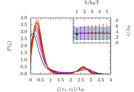
Fig. 11: The distributions $P(\zeta)$ are drawn for varying $h$ while the ligand is restrained at the peaking position of the friction from Fig. 7. The inset plots the respective first moment with second moment as errorbars evaluated from $P(\zeta)$ in the interval $[0,1]$. The average first moment is drawn as black line and the blueish shade illustrates the average second moment. (Color coding is adopted from Fig. 3.)

For development of a generalized Langevin model in the main text we expanded the coupling due to solvation potential up to first order in $\zeta(z_{1},z_{2})$. It was used to identify the force constant $\Omega=2\pi\Gamma\epsilon\equiv\xi/\tau$ to construct a harmonic coupling between reaction coordinate $q$ and auxiliary variable $x$ which directly relates to the noise strength of the corresponding GLE. For comparison to the friction values of the peaking friction from simulation the average and thus dominant distance $\epsilon$ between interface and the ligand has to be extracted from simulation. Therefore the ligand is fixed by an umbrella potential at the positions of each friction peak from simulations with increasing barrier height $h$ and the distribution $P_{h}(\zeta)$ is sampled. The distributions dependent on $h$ are plotted in Fig. 10 whereas all $P_{h}(\zeta)$ behave equivalently. The average and the standard deviation

$$\epsilon(h) =\langle\zeta\rangle$$ (21)

$$\Delta\epsilon(h) =\langle\zeta^{2}-\langle\zeta\rangle^{2}\rangle^{1/2}$$ (22)

are calculated within the interval $[0,1]$ in which interface and ligand interact. The values $\epsilon(h)$ are plotted in the inset of Fig. 10 with their standard deviation as errorbars. The black line draws the average $\epsilon=\langle\epsilon(h)\rangle_{h}=0.36$ which is used in the coupling strength. Similarly the average standard deviation $\delta\epsilon=\langle\Delta\epsilon(h)\rangle_{h}=0.24$ is plotted as blueish shade in Fig. 10.

References

- (1) P. Setny, R. Baron, P. Kekenes-Huskey, J. A. McCammon, and J. Dzubiella, Proc. Natl. Acad. Sci. (USA) 110, 1197 (2013)
- (2) J. Mondal, J. A. Morrone, and B. J. Berne, Proc. Natl. Acad. Sci. (USA) 110, 33 (2013)
- (3) S. H. Gellman, Chem. Rev. 97, 1231 (1997)
- (4) M. K. Gilson and H.-X. Zhou, Annu. Rev. Biophys. Biomol. Struct 36, 21 (2007)
- (5) H.-J. Woo and B. Roux, Proc. Natl. Acad. Sci. (USA) 102, 6825 (2005)
- (6) J. Wang, X. Zheng, Y. Yang, D. Drueckhammer, W. Yang, G. Verkhivker, and E. K. Wang, Phys. Rev. Lett. 99, 198101 (2007)
- (7) R. D. Head, M. L. Smythe, T. I. Oprea, C. L. Waller, S. M. Green, and G. R. Marshall, J. Am. Chem. Soc. 118, 3959 (1996)
- (8) J. A. McCammon, Curr. Opin. Struct. Biol. 8, 245 (1998)
- (9) A. C. Pan, D. W. Borhani, R. O. Dror, and D. E. Shaw, Drug Discov. Today 18, 667 (2013)
- (10) P. Tiwary, V. Limongello, M. Salvalaglio, and M. Parrinello, Proc. Natl. Acad. Sci. 112, 5 (2014)
- (11) D. Beece, L. Eisenstein, H. Frauenfelder, D.Good, M. C. Marden, L.Reinisch, A. Reynolds, L. Sorensen, and K. Yue, Biochemistry 19, 23 (1980)
- (12) R. F. Grote and J. T. Hynes, J. Chem. Phys. 73, 2715 (1980)
- (13) P. Hänggi, J. Stat. Phys. 30, 401 (1983)
- (14) W. Doster, Biophys. Chem. 17, 97 (1983)
- (15) H. Frauenfelder and P. G. Wolynes, Science 229, 4711 (1985)
- (16) P. R. Batista., G. Pandey, P. G. Pascutti, P. M. Bisch, D. Perahia, and C. H. Robert, J. Chem. Theory Comput. 7, 2348 (2011)
- (17) H. Ishikawa, K. Kwak, J. K. Chung, S. Kim, and M. D. Fayer, Proc. Natl. Acad. Sci (USA) 105, 25 (2008)
- (18) R. C. Bernardi, I. Cann, and K. Schulten, Biotech. for Biofuels 7, 83 (2014)
- (19) H.-X. Zhou, Biophys. J. 98, L15 (2010)
- (20) L. Cai and H.-X. Zhou, J. Chem. Phys. 134, 105101 (2011)
- (21) P. Setny, Z. Wang, L.-T. Cheng, B. Li, J. A. McCammon, and J. Dzubiella, Phys. Rev. Lett. 103, 187801 (2009)
- (22) D. Chandler, Nature 437, 640 (2005)
- (23) P. Setny, R. Baron, and J. A. McCammon, J. Chem. Theory Comput. 6, 2866 (2010)
- (24) D. L. Ermak and J. A. McCammon
- (25) P. Hänggi, P. Talkner, and M. Borkovec, Rev. Mod. Phys. 62, 251 (1990)
- (26) A. M. Ferrenberg and R. H. Swendsen, Phys. Rev. Lett. 63, 1195 (1989)
- (27) S. Kumar, J. M. Rosenberg, D. Bouzida, R. H. Swendsen, and P. A. Kollman, J. Comput. Chem. 13, 1011 (1992)
- (28) F. Zhu and G. Hummer, J. Comput. Chem. 33, 453 (2012)
- (29) A. J. F. Siegert, Phys. Rev. 81, 4 (1951)
- (30) G. H. Weiss, Adv. Chem. Phys. 13, 1 (1966)
- (31) P. Hänggi and P. Talkner, Phys. Rev. Lett. 51, 25 (1983)
- (32) G. Hummer, New Journal of Physics 7, 34 (2005)
- (33) M. Hinczewski, Y. von Hansen, J. Dzubiella, and R. R. Netz, J. Chem. Phys. 132, 245103 (2010)
- (34) H. Risken, The Fokker-Planck equation: Methods of solution and application, Springer, Berlin(1996)
- (35) N. G. van Kampen, Stochastic processes in physics and chemistry, North Holland, Amsterdam(2007)
- (36) E. Pollak and A. Berezhkovsii, J. Chem. Phys. 99 (2), 1344 (1993)
- (37) A. Berezhkovsii, A. Frishman, and E. Pollak, J. Chem. Phys. 101 (6), 4778 (1994)
- (38) P. J. Cregg, D. S. F. Crothers, and A. W. Wickstead, J. Appl. Phys. 76, 4900 (1994)
- (39) Y. P. Kalmykov, W. T. Coffey, and J. T. Waldron, J. Chem. Phys. 105, 2112 (1996)
- (40) A. Szabo, D. Shoup, S. H. Northrup, and J. A. McCammon, J. Chem. Phys. 77, 4484 (1982)
- (41) G. R. Bowman, V. S. Pande, and F. Noe, An introduction to markov state models and their application to long timescale molecular simulation, Springer: Dortrecht, The Netherlands(2014)
- (42) G. Hummer and A. Szabo, J. Phys. Chem. B 119(29), 9029 (2015)
- (43) J. Mondal, R. A. Friesner, and B. J. Berne, J. Chem. Theory Comput. 10, 5696 (2014)
- (44) P. E. Smith and W. F. van Gunsteren, Chem. Phys. Lett. 215, 4 (1993)
- (45) C. Vega and E. de Miquel, J. Chem. Phys. 126, 154707 (2007)