Low-energy hypernuclear spectra with microscopic particle-rotor model with relativistic point coupling hyperon-nucleon interaction

Abstract

We extend the microscopic particle-rotor model for hypernuclear low-lying states by including the derivative and tensor coupling terms in the point-coupling nucleon-$\Lambda$ particle ($N\Lambda$) interaction. Taking ${}^{13}_{~{}\Lambda}$C as an example, we show that a good overall description for excitation spectra is achieved with four sets of effective $N\Lambda$ interaction. We find that the $\Lambda$ hyperon binding energy decreases monotonically with increasing the strengths of the high-order interaction terms. In particular, the tensor coupling term decreases the energy splitting between the first $1/2^{-}$ and $3/2^{-}$ states and increases the energy splitting between the first $3/2^{+}$ and $5/2^{+}$ states in ${}^{13}_{~{}\Lambda}$C.

I Introduction

The spectroscopic data on low-lying states of light $\Lambda$ hypernuclei have been accumulated Hashimoto06 and more data on those of medium and heavy hypernuclei are expected to be obtained with the next-generation facilities such as J-PARC Tamura09 . Rich information on the hyperon-nucleon interaction in nuclear medium and the impurity effect of a $\Lambda$ particle on nuclear structure are contained in these data. Because hyperon-nucleon and hyperon-hyperon scattering experiments are difficult to perform, the structure of hypernuclei has been playing a vital role in order to shed light on baryon-baryon interactions. Such information is crucial in order to understand also neutron stars, in which hyperons may emerge in the inner part Glendenning00 . However, extracting information on baryon-baryon interactions from the spectroscopic data relies much on nuclear models.

In the past decades, several different types of theoretical models have been developed to study the structure of hypernuclei, including an ab-initio method abinitio , a cluster model Motoba83 ; Hiyama99 ; Bando90 ; Hiyama03 ; Cravo02 ; Suslov04 ; Shoeb09 , a shell model Dalitz78 ; Gal71 ; Millener , the anti-symmetrized molecular dynamics (AMD) Isaka11 ; Isaka11-2 ; Isaka12 ; Isaka13 , self-consistent mean-field approach Zhou07 ; Win08 ; Schulze10 ; Win11 ; Lu11 ; Weixia14 ; Li13 ; Lu14 ; HY14 and the generator coordinator method (GCM) based on energy density functionals Mei15-2 . In recent years, we have also developed a microscopic particle rotor model (MPRM) for hypernuclear low-lying states based on the beyond-mean-field approach Mei2014 ; Mei2015 . In contrast to the GCM for the whole hypernuclei Mei15-2 , where the wave function of the hypernuclear states is given as a superposition of hypernuclear mean-field states, the hypernuclear states in the MPRM are constructed by coupling a hyperon to low-lying states of the core nucleus. The MPRM provides a convenient way to analyze the components of hypernuclear wave function and has been applied to study the low-lying states of ${}^{9}_{\Lambda}$Be Mei2014 , ${}^{13}_{~{}\Lambda}$C, ${}^{21}_{~{}\Lambda}$Ne and ${}^{155}_{\Lambda}$Sm hypernuclei Mei2015 . For the sake of simplicity, only the leading-order four-fermion coupling terms of scalar and vector types were adopted for the $N\Lambda$ effective interaction in these studies.

The aim of this paper is to extend the previous calculations by implementing the higher-order derivative and tensor $N\Lambda$ interaction terms in the point-coupling interaction Tanimura2012 . The derivative terms simulate to some extent the finite-range character of $N\Lambda$ interaction and these terms are expected to be more pronounced in light hypernuclei Hiyama14 . On the other hand, the tensor $N\Lambda$ interaction is important to reproduce a small hyperon spin-orbit splitting in $\Lambda$ hypernuclei Noble80 . It is therefore important to assess the effect of these terms on hypernuclear low-lying states.

The paper is organized as follows. In Sec. II, we present the main formulas of the microscopic PRM for $\Lambda$ hypernuclei with the full point-coupling effective $N\Lambda$ interaction. In Sec. III, we show the results for hypernuclear low-lying states in ${}^{13}_{~{}\Lambda}$C and discuss the influence of the higher-order terms on the energy spectra. We then summarize the paper in Sec. IV.

II Microscopic particle-rotor model for $\Lambda$ hypernuclei

In this paper, we consider a single-$\Lambda$ hypernucleus and describe the hypernuclear low-lying states using the microscopic particle-rotor model (MPRM). Since the detailed formulas for the MPRM have been given in Refs. Mei2014 ; Mei2015 , we give here only the main formulas of this approach. To this end, we put a particular emphasis on the implementation of the higher-order $N\Lambda$ interaction terms.

The basic idea of the MPRM is to construct a hypernuclear wave function by coupling the valence $\Lambda$ hyperon to the low-lying states of nuclear core in the laboratory frame, that is,

$$\displaystyle\Psi_{JM}(\mbox{\boldmath$r$},\{\mbox{\boldmath$r$}_{i}\}) = \sum_{n,j,\ell,I}{\mathscr{R}}_{j\ell nI}(r){\mathscr{F}}^{JM}_{j\ell nI}(\hat{\mbox{\boldmath$r$}},\{\mbox{\boldmath$r$}_{i}\}),$$ (1)

with

$${\mathscr{F}}^{JM}_{j\ell nI}(\hat{\mbox{\boldmath$r$}},\{\mbox{\boldmath$r$}_{i}\})=[{\mathscr{Y}}_{j\ell}(\hat{\mbox{\boldmath$r$}})\otimes\Phi_{nI}(\{\mbox{\boldmath$r$}_{i}\})]^{(JM)},$$ (2)

where $r$ and $\mbox{\boldmath$r$}_{i}$ are the coordinates of the $\Lambda$ hyperon and the nucleons, respectively. Here, $J$ is the angular momentum for the whole system, while $M$ is its projection onto the $z$-axis in the laboratory frame. ${\mathscr{Y}}_{j\ell}(\hat{\mbox{\boldmath$r$}})$ is the spin-angular wave function for the $\Lambda$ hyperon. $|\Phi_{nI}\rangle$ is the wave functions for the low-lying states of the core nucleus, where $I$ represents the angular momentum of the core state and $n=1,2,\ldots$ distinguish different core states with the same angular momentum $I$. In the MPRM, the core states $|\Phi_{nI}\rangle$ are constructed with the quantum-number projected GCM approach Mei2014 ; Mei2015 . For convenience, hereafter we introduce the shorthanded notation $k=\{j\ell nI\}$ to represent different channels.

In Eq. (1), ${\mathscr{R}}_{k}(r)$ is the radial wave function for the $\Lambda$-particle. In the relativistic approach, it is given as a four-component Dirac spinor

$${\mathscr{R}}_{k}(r)=\begin{pmatrix}f_{k}(r)\\ ig_{k}(r)\mbox{\boldmath$\sigma$}\cdot\hat{\mbox{\boldmath$r$}}\end{pmatrix}.$$ (3)

We assume that the Hamiltonian $\hat{H}$ for the whole $\Lambda$ hypernucleus is given as

$$\hat{H}=\hat{T}_{\Lambda}+\hat{H}_{\rm c}+\sum^{A_{c}}_{i=1}\hat{V}^{N\Lambda}(\mbox{\boldmath$r$},\mbox{\boldmath$r$}_{i}).$$ (4)

Here $\displaystyle\hat{T}_{\Lambda}=-i\mbox{\boldmath$\alpha$}\cdot\nabla_{\Lambda}+\gamma^{0}m_{\Lambda}$ is the relativistic kinetic energy of $\Lambda$ hyperon, where $m_{\Lambda}$ is the mass of $\Lambda$ particle, and $\alpha$ and $\gamma^{0}$ are the Dirac matrices. $\hat{H}_{c}$ is the many-body Hamiltonian for the core nucleus Buvenich02 , with which the core state $|\Phi_{nI}\rangle$ satisfies $\hat{H}_{c}|\Phi_{nI}\rangle=E_{nI}|\Phi_{nI}\rangle$. The last term in Eq. (4) represents the $N\Lambda$ interaction term between the valence $\Lambda$ particle and the nucleons in the core nucleus, where $A_{c}$ is the mass number of the core nucleus.

We construct the $N\Lambda$ interaction $\hat{V}^{N\Lambda}$ based on the relativistic point-coupling model Tanimura2012 , in which the energy functional for the $N\Lambda$ interaction reads

$$E^{(N\Lambda)}_{\rm int}= \int d\mbox{\boldmath$r$}\Big{[}\alpha_{S}^{N\Lambda}\rho_{S}(\mbox{\boldmath$r$})\rho^{\Lambda}_{S}(\mbox{\boldmath$r$})+\alpha_{V}^{N\Lambda}\rho_{V}(\mbox{\boldmath$r$})\rho^{\Lambda}_{V}(\mbox{\boldmath$r$})$$

$$+\delta_{S}^{N\Lambda}\rho_{S}(\mbox{\boldmath$r$})\Delta\rho^{\Lambda}_{S}(\mbox{\boldmath$r$})+\delta_{V}^{N\Lambda}\rho_{V}(\mbox{\boldmath$r$})\Delta\rho^{\Lambda}_{V}(\mbox{\boldmath$r$})$$

$$+\alpha_{T}^{N\Lambda}\rho^{\Lambda}_{T}(\mbox{\boldmath$r$})\rho_{V}(\mbox{\boldmath$r$})\Big{]}.$$ (5)

Here $\rho_{S}$, $\rho_{V}$ and $\rho_{T}$ are the scalar, the vector and the tensor densities defined in Ref. Tanimura2012 , respectively. Taking the second functional derivative of Eq. (II) with respect to the densities Ring80 ,

$$\hat{V}^{N\Lambda}(\mbox{\boldmath$r$},\mbox{\boldmath$r$}_{i})= \frac{\delta^{2}E[\rho]}{\delta\rho^{\Lambda}_{S}(\mbox{\boldmath$r$})\delta\rho_{S}(\mbox{\boldmath$r$}_{i})}+\frac{\delta^{2}E[\rho]}{\delta\rho^{\Lambda}_{V}(\mbox{\boldmath$r$})\delta\rho_{V}(\mbox{\boldmath$r$}_{i})}$$

$$+\frac{\delta^{2}E[\rho]}{\delta\rho^{\Lambda}_{T}(\mbox{\boldmath$r$})\delta\rho_{V}(\mbox{\boldmath$r$}_{i})},$$ (6)

we obtain the following form for the $N\Lambda$ effective interaction

$$\hat{V}^{N\Lambda}=\hat{V}^{N\Lambda}_{\rm S}+\hat{V}^{N\Lambda}_{\rm V}+\hat{V}^{N\Lambda}_{\rm Ten},$$ (7)

where the scalar, vector and tensor types of coupling terms read

$$\hat{V}^{N\Lambda}_{\rm S}(\mbox{\boldmath$r$},\mbox{\boldmath$r$}_{i})= \alpha_{S}^{N\Lambda}\gamma^{0}_{\Lambda}\delta(\mbox{\boldmath$r$}-\mbox{\boldmath$r$}_{i})\gamma^{0}_{N}+\delta_{S}^{N\Lambda}\gamma^{0}_{\Lambda}\Big{[}\overleftarrow{\nabla}^{2}\delta(\mbox{\boldmath$r$}-\mbox{\boldmath$r$}_{i})$$

$$+\delta(\mbox{\boldmath$r$}-\mbox{\boldmath$r$}_{i})\overrightarrow{\nabla}^{2}+2\overleftarrow{\nabla}\cdot\delta(\mbox{\boldmath$r$}-\mbox{\boldmath$r$}_{i})\overrightarrow{\nabla}\Big{]}\gamma^{0}_{N}$$ (8)

$$\hat{V}^{N\Lambda}_{\rm V}(\mbox{\boldmath$r$},\mbox{\boldmath$r$}_{i})= \alpha_{V}^{N\Lambda}\delta(\mbox{\boldmath$r$}-\mbox{\boldmath$r$}_{i})+\delta_{V}^{N\Lambda}\Big{[}\overleftarrow{\nabla}^{2}\delta(\mbox{\boldmath$r$}-\mbox{\boldmath$r$}_{i})$$

$$+\delta(\mbox{\boldmath$r$}-\mbox{\boldmath$r$}_{i})\overrightarrow{\nabla}^{2}+2\overleftarrow{\nabla}\cdot\delta(\mbox{\boldmath$r$}-\mbox{\boldmath$r$}_{i})\overrightarrow{\nabla}\Big{]}$$ (9)

$$\hat{V}^{N\Lambda}_{\rm Ten}(\mbox{\boldmath$r$},\mbox{\boldmath$r$}_{i})= i\alpha_{T}^{N\Lambda}\gamma^{0}_{\Lambda}\Big{[}\overleftarrow{\nabla}\delta(\mbox{\boldmath$r$}-\mbox{\boldmath$r$}_{i})+\delta(\mbox{\boldmath$r$}-\mbox{\boldmath$r$}_{i})\overrightarrow{\nabla}\Big{]}\cdot\mbox{\boldmath$\alpha$}.$$ (10)

Here,$\overrightarrow{\nabla}$ and $\overleftarrow{\nabla}$ are understood to act on the right and left hands sides of the $\Lambda$ hyperon coordinates, respectively. Vice versa, Eq. (II) can be obtained from the above effective $N\Lambda$ interaction (see Appendix A). We note that similar terms appear in the chiral hyperon-nucleon interaction Polinder06 , in which the non-derivative four-fermion coupling corresponds to the contact leading-order (LO) term.

With Eqs. (1) and (4), the radial wave function ${\mathscr{R}}_{k}(r)$ in Eq. (3) and the energy $E_{J}$ for each hypernuclear state are obtained by solving the following coupled-channels equations,

$$\left(\frac{d}{dr}-\frac{\kappa-1}{r}\right)g_{k}(r)+(E_{nI}-E_{J})f_{k}(r)$$

$$+\sum_{k^{\prime}}U^{kk^{\prime}}_{T}(r)g_{k^{\prime}}(r)+\sum_{k^{\prime}}\left[U^{kk^{\prime}}_{V}(r)+U^{kk^{\prime}}_{S}(r)\right]f_{k^{\prime}}(r)=0,$$ (11a)

$$\left(\frac{d}{dr}+\frac{\kappa+1}{r}\right)f_{k}(r)-(E_{nI}-2m_{\Lambda}-E_{J})g_{k}(r)$$

$$-\sum_{k^{\prime}}U^{kk^{\prime}}_{T}(r)f_{k^{\prime}}(r)-\sum_{k^{\prime}}\left[U^{kk^{\prime}}_{V}(r)-U^{kk^{\prime}}_{S}(r)\right]g_{k^{\prime}}(r)=0,$$ (11b)

where $\kappa$ is defined as $\kappa=(-1)^{j+\ell+1/2}(j+1/2)$. The coupling potentials between different channels are given by

$$U^{kk^{\prime}}_{\mathrm{S}}(r)\equiv \langle{\mathscr{F}}^{JM}_{jlnI}|\sum_{i=1}^{A_{c}}\hat{V}_{\mathrm{S}}^{N\Lambda}(\mbox{\boldmath$r$},\mbox{\boldmath$r$}_{i})|{\mathscr{F}}^{JM}_{j^{\prime}l^{\prime}n^{\prime}I^{\prime}}\rangle$$ (12a)

$$U^{kk^{\prime}}_{\mathrm{V}}(r)\equiv \langle{\mathscr{F}}^{JM}_{jlnI}|\sum_{i=1}^{A_{c}}\hat{V}_{\mathrm{V}}^{N\Lambda}(\mbox{\boldmath$r$},\mbox{\boldmath$r$}_{i})|{\mathscr{F}}^{JM}_{j^{\prime}l^{\prime}n^{\prime}I^{\prime}}\rangle$$ (12b)

$$U^{kk^{\prime}}_{T}(r)\equiv \langle{\mathscr{F}}^{JM}_{jlnI}|\sum_{i=1}^{A_{c}}\hat{V}_{\mathrm{T}}^{N\Lambda}(\mbox{\boldmath$r$},\mbox{\boldmath$r$}_{i})\cdot\mbox{\boldmath$\sigma$}|{\mathscr{F}}^{JM}_{j^{\prime}\tilde{l}^{\prime}n^{\prime}I^{\prime}}\rangle,$$ (12c)

with

$$\hat{V}^{N\Lambda}_{\mathrm{T}}\equiv\alpha_{T}^{N\Lambda}\left[\overleftarrow{\nabla}\delta(\mbox{\boldmath$r$}-\mbox{\boldmath$r$}_{i})+\delta(\mbox{\boldmath$r$}-\mbox{\boldmath$r$}_{i})\overrightarrow{\nabla}\right].$$ (13)

By expanding each of the large $f_{k}(r)$ and small $g_{k}(r)$ components of the Dirac spinors, Eq.(3), in terms of the radial function $R_{\alpha l}(r)$ of a spherical harmonic oscillator, that is,

$$f_{k}(r)= \sum_{\alpha=1}^{f^{(k)}_{max}}F_{k\alpha}R^{k}_{\alpha l}(r),$$ (14a)

$$g_{k}(r)= \sum_{\alpha=1}^{g^{(k)}_{max}}G_{k\alpha}R^{k}_{\alpha\tilde{l}}(r),$$ (14b)

with $l=j\pm 1/2$ and $\tilde{l}=j\mp 1/2$, the coupled-channels equations (11), (11) are transformed into a real symmetric matrix equation,

$$\sum_{\alpha^{\prime},k^{\prime}}\begin{pmatrix}A^{kk^{\prime}}_{\alpha\alpha^{\prime}}+V^{kk^{\prime}}_{\alpha\alpha^{\prime}}+S^{kk^{\prime}}_{\alpha\alpha^{\prime}}&B^{kk^{\prime}}_{\alpha\alpha^{\prime}}+T^{kk^{\prime}}_{\alpha\alpha^{\prime}}\\ B^{kk^{\prime}}_{\alpha\alpha^{\prime}}+T^{kk^{\prime}}_{\alpha\alpha^{\prime}}&C^{kk^{\prime}}_{\alpha\alpha^{\prime}}+V^{kk^{\prime}}_{\alpha\alpha^{\prime}}-S^{kk^{\prime}}_{\alpha\alpha^{\prime}}\end{pmatrix}\begin{pmatrix}F^{k^{\prime}}_{\alpha^{\prime}}\\ G^{k^{\prime}}_{\alpha^{\prime}}\end{pmatrix}$$

$$=E_{J}\begin{pmatrix}F^{k}_{\alpha}\\ G^{k}_{\alpha}\end{pmatrix}.$$ (15)

The dimension of the matrix is $\displaystyle\sum_{k}f^{(k)}_{max}+g^{(k)}_{max}$, where $k$ represents different channels. In Eq. (II), the matrix elements are given by

$$A^{kk^{\prime}}_{\alpha\alpha^{\prime}}= \langle R^{k}_{\alpha l}(r)|E_{nI}|R^{k^{\prime}}_{\alpha^{\prime}l^{\prime}}(r)\rangle\delta_{k,k^{\prime}}$$ (16a)

$$B^{kk^{\prime}}_{\alpha\alpha^{\prime}}= \langle R^{k}_{\alpha l}(r)|\frac{d}{dr}-\frac{\kappa-1}{r}|R^{k^{\prime}}_{\alpha^{\prime}\tilde{l}^{\prime}}(r)\rangle\delta_{k,k^{\prime}}$$ (16b)

$$C^{kk^{\prime}}_{\alpha\alpha^{\prime}}= \langle R^{k}_{\alpha\tilde{l}}(r)|(E_{nI}-2m_{\Lambda})|R^{k^{\prime}}_{\alpha^{\prime}\tilde{l}^{\prime}}(r)\rangle\delta_{k,k^{\prime}}$$ (16c)

$$V^{kk^{\prime}}_{\alpha\alpha^{\prime}}= \langle R^{k}_{\alpha l}(r)|U^{kk^{\prime}}_{V}(r)|R^{k^{\prime}}_{\alpha^{\prime}l^{\prime}}(r)\rangle$$

$$= (-1)^{j^{\prime}+I+J}\sum_{\lambda}\left\{\begin{matrix}J&I&j\\ \lambda&j^{\prime}&I^{\prime}\end{matrix}\right\}\langle j\ell||Y_{\lambda}||j^{\prime}\ell^{\prime}\rangle$$

$$\times\int r^{2}dr\rho^{nIn^{\prime}I^{\prime}}_{\lambda,V}(r)\Big{\{}\alpha_{V}^{N\Lambda}R^{k}_{\alpha l}(r)R^{k^{\prime}}_{\alpha^{\prime}l^{\prime}}(r)+\delta_{V}^{N\Lambda}$$

$$\left[\frac{1}{r^{2}}\frac{d}{dr}(r^{2}\frac{d}{dr})-\frac{\lambda(\lambda+1)}{r^{2}}\right]\left[R^{k}_{\alpha l}(r)R^{k^{\prime}}_{\alpha^{\prime}l^{\prime}}(r)\right]\Big{\}}$$ (16d)

$$S^{kk^{\prime}}_{\alpha\alpha^{\prime}}= \langle R^{k}_{\alpha l}(r)|U^{kk^{\prime}}_{S}(r)|R^{k^{\prime}}_{\alpha^{\prime}l^{\prime}}(r)\rangle$$

$$= (-1)^{j^{\prime}+I+J}\sum_{\lambda}\left\{\begin{matrix}J&I&j\\ \lambda&j^{\prime}&I^{\prime}\end{matrix}\right\}\langle j\ell||Y_{\lambda}||j^{\prime}\ell^{\prime}\rangle$$

$$\times\int r^{2}dr\rho^{nIn^{\prime}I^{\prime}}_{\lambda,S}(r)\Big{\{}\alpha_{S}^{N\Lambda}R^{k}_{\alpha l}(r)R^{k^{\prime}}_{\alpha^{\prime}l^{\prime}}(r)+\delta_{S}^{N\Lambda}$$

$$\left[\frac{1}{r^{2}}\frac{d}{dr}(r^{2}\frac{d}{dr})-\frac{\lambda(\lambda+1)}{r^{2}}\right]\left[R^{k}_{\alpha l}(r)R^{k^{\prime}}_{\alpha^{\prime}l^{\prime}}(r)\right]\Big{\}}$$ (16e)

$$T^{kk^{\prime}}_{\alpha\alpha^{\prime}}= \langle R^{k}_{\alpha l}(r)|U^{kk^{\prime}}_{T}(r)|R^{k^{\prime}}_{\alpha^{\prime}\tilde{l}^{\prime}}(r)\rangle$$

$$= -\alpha_{T}^{N\Lambda}(-1)^{j+I^{\prime}+J}\sum_{\lambda}\left\{\begin{matrix}J&I&j\\ \lambda&j^{\prime}&I^{\prime}\end{matrix}\right\}\int r^{2}dr\rho^{nIn^{\prime}I^{\prime}}_{\lambda,V}(r)$$

$$\times\Big{\{}\Big{[}\frac{dR^{k}_{\alpha l}(r)}{dr}+\frac{\kappa+1}{r}R^{k}_{\alpha l}(r)\Big{]}R^{k^{\prime}}_{\alpha^{\prime}\tilde{l}^{\prime}}(r)\langle j\tilde{\ell}||Y_{\lambda}||j^{\prime}\tilde{\ell^{\prime}}\rangle$$

$$+\Big{[}\frac{dR^{k^{\prime}}_{\alpha^{\prime}\tilde{l}^{\prime}}(r)}{dr}-\frac{\kappa^{\prime}-1}{r}R^{k^{\prime}}_{\alpha^{\prime}\tilde{l}^{\prime}}(r)\Big{]}R^{k}_{\alpha l}(r)\langle j\ell||Y_{\lambda}||j^{\prime}\ell^{\prime}\rangle\Big{\}}.$$ (16f)

See Appendices B and C for the derivation of Eqs. (16e) and (16f), respectively. In Eq. (16), $\rho^{nIn^{\prime}I^{\prime}}_{\lambda,V}(r)$ and $\rho^{nIn^{\prime}I^{\prime}}_{\lambda,S}(r)$ are the reduced vector and scalar transition densities, respectively, between the nuclear initial state $|\Phi_{n^{\prime}I^{\prime}}\rangle$ and the final state $|\Phi_{nI}\rangle$ defined as

$$\rho^{nIn^{\prime}I^{\prime}}_{\lambda,V}(r) = \langle\Phi_{nI}||\sum\limits_{i=1}^{A_{c}}\frac{\delta(r-r_{i})}{r_{i}r}Y_{\lambda}(\hat{\mbox{\boldmath$r$}}_{i})||\Phi_{n^{\prime}I^{\prime}}\rangle,$$ (17a)

$$\rho^{nIn^{\prime}I^{\prime}}_{\lambda,S}(r) = \langle\Phi_{nI}||\sum\limits_{i=1}^{A_{c}}\gamma^{0}_{i}\frac{\delta(r-r_{i})}{r_{i}r}Y_{\lambda}(\hat{\mbox{\boldmath$r$}}_{i})||\Phi_{n^{\prime}I^{\prime}}\rangle.$$ (17b)

The detailed expressions for the transition densities can be found in Ref. Yao15 .

Table 1: The four parameter sets of relativisitc point-coupling $N\Lambda$ interaction proposed in Ref. Tanimura2012 .

	PCY-S1	PCY-S2	PCY-S3	PCY-S4
$\alpha_{S}^{N\Lambda}$ (MeV-2)	$-2.0305\times 10^{-4}$	$-4.2377\times 10^{-5}$	$-2.0197\times 10^{-4}$	$-1.8594\times 10^{-4}$
$\alpha_{V}^{N\Lambda}$ (MeV-2)	$~{}~{}1.6548\times 10^{-4}$	$~{}~{}1.4268\times 10^{-5}$	$~{}~{}1.6449\times 10^{-4}$	$~{}~{}1.4981\times 10^{-4}$
$\delta_{S}^{N\Lambda}$ (MeV-4)	$~{}~{}2.2929\times 10^{-9}$	$~{}~{}1.2986\times 10^{-9}$	$~{}~{}2.3514\times 10^{-9}$	$-1.9958\times 10^{-10}$
$\delta_{V}^{N\Lambda}$ (MeV-4)	$-2.3872\times 10^{-9}$	$-1.3850\times 10^{-9}$	$-2.4993\times 10^{-9}$	$~{}~{}~{}~{}0$
$\alpha_{T}^{N\Lambda}$ (MeV-3)	$-1.0603\times 10^{-7}$	$~{}~{}~{}~{}0$	$-4.082\times 10^{-9}$	$-5.5322\times 10^{-8}$

Figure 1: (Color online) The low-energy excitation spectra of ${}^{13}_{~{}\Lambda}$C obtained with the microscopic particle-rotor model with (b)PCY-S1, (c)PCY-S2, (d)PCY-S3 and (e)PCY-S4. Fig. 1(f) shows the spectrum taken from Ref. Mei2015 , which was obtained by including only the leading-order (LO) $N\Lambda$ interaction. The experimental data shown in Fig. 1(a) are taken from Refs. Ajimura01 ; Kohri02 . The numbers with the arrows indicate the B($E2$) value for the $3/2^{+}_{1}\rightarrow 1/2^{+}_{1}$ and the $9/2^{+}_{1}\rightarrow 5/2^{+}_{1}$ transitions, given in units of $e^{2}$ fm⁴. The dominant component of several hypernuclear states, together with its weight (in percent), is also given.

Figure 2: (Color online) Same as the Fig. 1, but with the scaled $N\Lambda$ interaction, in which the scaling factor is determined for each parameter set to reproduce the empirical $\Lambda$ binding energy of ${}^{13}_{~{}\Lambda}$C.

III Application to ${}^{13}_{~{}\Lambda}$C

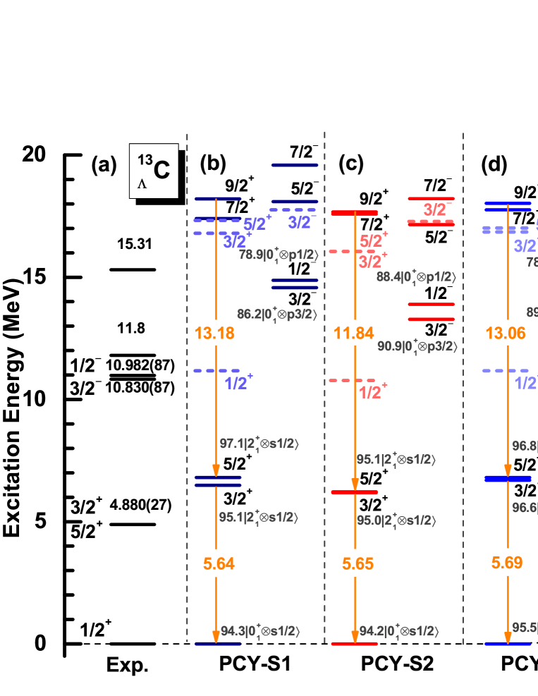
Let us now apply the MPRM with the higher-order $N\Lambda$ interaction to ${}^{13}_{~{}\Lambda}$C, for which several low-lying states have been observed experimentally Ajimura01 ; Kohri02 . To this end, we first generate several low-lying states of the core nucleus ¹²C with a quantum-number projected GCM calculation, where the mean-field configurations are obtained from deformation constrained relativistic mean-field plus BCS calculation using the point-coupling PC-F1 for the effective nucleon-nucleon interaction Buvenich02 . A zero-range pairing force supplemented with a smooth cutoff is adopted to treat the pairing correlation among the nucleons. Axial symmetry and time-reversal invariance are imposed in the mean-field calculations. The Dirac spinor for each nucleon state is expanded on a harmonic oscillator basis with 10 shells. More numerical details have been presented in Refs. Mei2014 ; Mei2015 . The wave functions and the energies of the low-lying states of ¹²C are then used to calculate the scalar and vector transition densities given by Eq. (17) as well as the matrix elements in Eq. (II). The radial wave function for the spherical harmonic oscillator basis with 18 shells are used to expand the radial part of the hypernuclear wave function, ${\mathscr{R}}_{k}(r)$. We use the effective $N\Lambda$ interaction with the PCY-S1, PCY-S2, PCY-S3 and PCY-S4 parameter sets, which were determined by fitting to the experimental data of $\Lambda$ binding energies from light to heavy mass hypernuclei Tanimura2012 . We list these parameters in Table 1. Notice that PCY-S2 and PCY-S4 do not include the tensor and the derivative terms, respectively. Notice also that PCY-S3 was obtained by excluding the spin-orbit splitting of the 1p state of $\Lambda$ in ${}^{16}_{\Lambda}$O from the fitting, and the strength of the tensor coupling is considerably smaller than that in PCY-S1.

III.1 Low-energy spectra

Figures  1(b)-(e) show the calculated low-energy spectra of ${}^{13}_{~{}\Lambda}$C with the higher order $N\Lambda$ interaction, in comparison with the experimental data as well as with the results of Ref. Mei2015 obtained only with the leading-order $N\Lambda$ interaction. One can see that the calculated energy splitting between the $1/2^{-}$ and $3/2^{-}$ states, as well as that between the $5/2^{+}$ and $3/2^{+}$ states, are clearly different among the four different parameter sets, although the main structures of the low-lying states are the same. That is, the splitting between the $1/2^{-}_{1}$ and $3/2^{-}_{1}$ with PCY-S1 and PCY-S4 forces are smaller than that with PCY-S2 and PCY-S3 forces and much close to the experiment data. The splitting between the $5/2^{+}$ and $3/2^{+}$ states by the PCY-S1 are much larger than that by the other parameter sets. In other words, the fine structure of the hypernuclear low-lying states reflects the impact of the $N\Lambda$ interaction beyond the leading order. We have performed similar calculations for ${}^{9}_{\Lambda}$Be, and have found that the effects of the derivative and the tensor terms are similar to those in ${}^{13}_{\Lambda}$C. Notice that even though the tensor term is absent in the PCY-S2 force, a good description is still acieved by largely deviating from the expected relations of a naive quark model, that is, $\alpha^{N\Lambda}=\frac{2}{3}\alpha^{NN}$ etc. Toki94 . We will further discuss the role of the higher order terms in $N\Lambda$ interaction in the next subsections. In particular, we will demonstrate that the tensor term plays an important role if the expected relations of the naive quark model are maintained.

In Fig.1, the $E2$ transition strengths between the low-lying states of ${}^{13}_{~{}\Lambda}$C are also presented. One can see that the $E2$ transition strengths do not much vary with the four $N\Lambda$ effective interactions and are close to those with the LO interaction.

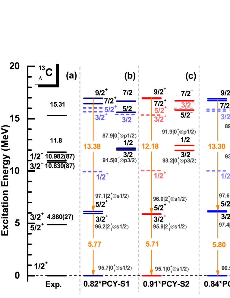
Given the fact that all the four parameter sets of the effective $N\Lambda$ interaction were adjusted to $\Lambda$ binding energy of hypernuclei at the mean-field level Tanimura2012 , the use of these forces in the present MPRM calculation overestimates the $\Lambda$ binding energy of ${}^{13}_{~{}\Lambda}$C. That is, the $\Lambda$ binding energy of ${}^{13}_{~{}\Lambda}$C defined as the energy difference between the $0^{+}_{1}$ state of ¹²C and the $1/2^{+}_{1}$ state of ${}^{13}_{~{}\Lambda}$C are calculated to be $15.72$, $13.63$, $15.42$ and $13.22$ MeV using the PCY-S1, PCY-S2, PCY-S3 and PCY-S4 sets of $N\Lambda$ interaction, respectively, while the empirical value is $B^{\mathrm{exp}.}_{\Lambda}=11.38\pm 0.05$ MeVHashimoto06 . If we want to reproduce the $\Lambda$ binding energy within this approach, we need to scale all the coupling strengths in the parameters of the $N\Lambda$ interaction by $18\%$, $9\%$, $16\%$ and $8\%$ for PCY-S1, PCY-S2, PCY-S3 and PCY-S4, respectively.

Figure 2 shows the calculated low-lying spectra of ${}^{13}_{~{}\Lambda}$C with those scaled effective $N\Lambda$ interactions. It is shown that the predicted low-lying excitation spectrum of ${}^{13}_{~{}\Lambda}$C is slightly compressed and the $E2$ transition strengths are somewhat increased. On the other hand, the energy splitting between the $1/2^{-}_{1}$ and $3/2^{-}_{1}$ states remains large by the PCY-S2 and PCY-S3 forces, while it is reduced from 303.7 keV (253.7 keV) to 161.5 keV(206.3 keV) after scaling the coupling strengths for the PCY-S1 (PCY-S4) interaction. Due to the slightly weaker $N\Lambda$ interaction, the configuration mixing for the $1/2^{+}_{1}$, $3/2^{+}_{1}$, $5/2^{+}_{1}$, $1/2^{-}_{1}$ and $3/2^{-}_{1}$ states becomes slightly reduced for all the four parameter sets.

III.2 Effects of the derivative coupling terms

Figure 3: (Color online) (a) and (c): Contour plots for the absolute value of the difference between the theoretical and the experimental hyperon binding energies of ${}^{13}_{~{}\Lambda}$C hypernucleus as a function of the coupling strength parameters ($\delta^{N\Lambda}_{S}$, $\delta^{N\Lambda}_{V}$) and ($\delta^{N\Lambda}_{S}$, $\alpha^{N\Lambda}_{S}$), respectively. In the former, $\alpha^{N\Lambda}_{V}$ and $\alpha^{N\Lambda}_{S}$ are fixed to the same values as in PCY-S2, while in the latter, the value of $\alpha^{N\Lambda}_{V}$ and $\delta^{N\Lambda}_{V}$ is determined for each ($\alpha^{N\Lambda}_{S},\delta^{N\Lambda}_{S}$) so as to keep the ratios $\alpha^{N\Lambda}_{V}/\alpha^{N\Lambda}_{S}$ and $\delta^{N\Lambda}_{V}/\delta^{N\Lambda}_{S}$ to be the same as those for PCY-S2. (b) and (d): Low-lying states in ${}^{13}_{~{}\Lambda}$C calculated with the strength parameters denoted by the dots in the panels (a) and (c), respectively.

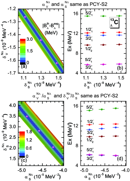
We now examine the effect of the derivative coupling terms on the $\Lambda$ binding energy. To this end, we fix the coupling strengths for the leading order terms ($\alpha^{N\Lambda}_{V},\alpha^{N\Lambda}_{S}$) to be the same values as those in the PCY-S2 force and study the $\Lambda$ binding energy as a function of the coupling strengths ($\delta^{N\Lambda}_{V}$, $\delta^{N\Lambda}_{S}$) of the derivative terms. Notice that the tensor coupling is absent in PCY-S2, so that we can isolate the effect of the derivative terms. The results are shown in Fig. 3(a). A clear linear correlation is observed between $\delta^{N\Lambda}_{V}$ and $\delta^{N\Lambda}_{S}$. By selecting three sets of $(\delta^{N\Lambda}_{V},\delta^{N\Lambda}_{S})$ along the valley in Fig. 3(a), we calculate the low-lying states of ${}^{13}_{~{}\Lambda}$C and show them in Fig. 3(b). One can see that the low-lying states are similar to each other. This implies that the coupling strengths $(\delta^{N\Lambda}_{V},\delta^{N\Lambda}_{S})$ may not be uniquely determined by the energies of hypernuclear low-lying states.

Figure 4: (Color online) (a): The $\Lambda$ binding energy in ${}^{13}_{~{}\Lambda}$C as a function of $|\delta^{N\Lambda}_{S}+\delta^{N\Lambda}_{V}|$, while keeping the same values of $\alpha^{N\Lambda}_{S}$, $\alpha^{N\Lambda}_{V}$, $\alpha^{N\Lambda}_{T}$ and $\delta^{N\Lambda}_{V}/\delta^{N\Lambda}_{S}$ as the original values for the PCY-S1, PCY-S2,PCY-S3, and PCY-S4 parameter sets. $B_{\Lambda}$ with the original value of $\delta^{N\Lambda}_{S}$ and $\delta^{N\Lambda}_{V}$ is denoted by the open circles for each parameter set. The experimental value is denoted by the thin solid line. (b): The energy levels of the low-lying states as a function of $|\delta^{N\Lambda}_{S}+\delta^{N\Lambda}_{V}|$ for the PCY-S1 parameter set. (c) and (d): The energy splitting between the $5/2^{+}_{1}$ and $3/2^{+}_{1}$ states and that between the $1/2^{-}_{1}$ and $3/2^{-}_{1}$ states, respectively, as a function of $|\delta^{N\Lambda}_{S}+\delta^{N\Lambda}_{V}|$.

Figure 5: (Color online) Same as Fig. 4, but as a function of the tensor coupling strength $|\alpha^{N\Lambda}_{T}|(=-\alpha^{N\Lambda}_{T})$ for the PCY-S1 and PCY-S4 forces.

Since the vector coupling strengths $\alpha^{N\Lambda}_{V}$ and $\delta^{N\Lambda}_{V}$ are linearly correlated with the corresponding scalar coupling strengths $\alpha^{N\Lambda}_{S}$ and $\delta^{N\Lambda}_{S}$, respectively, we next keep the ratios of $\alpha^{N\Lambda}_{V}/\alpha^{N\Lambda}_{S}$ and $\delta^{N\Lambda}_{V}/\delta^{N\Lambda}_{S}$ to be the same as those in PCY-S2 force and calculate the $\Lambda$ binding energy as well as the low-lying spectrum as a function of $\alpha^{N\Lambda}_{S}$ and $\delta^{N\Lambda}_{S}$ as shown in Fig. 3(c) and (d), respectively. It is shown that the parameters $\delta^{N\Lambda}_{S}$ and $\alpha^{N\Lambda}_{S}$ are also linearly correlated when these are fitted to the $\Lambda$ binding energy in ${}^{13}_{~{}\Lambda}$C (see Fig. 3(c)).

Notice that the difference between the vector transition density $\rho^{nIn^{\prime}I^{\prime}}_{\lambda,V}(r)$ and the scalar transition density $\rho^{nIn^{\prime}I^{\prime}}_{\lambda,S}(r)$ in the low-lying states of ¹²C is small (see Fig.4 in Ref. Mei2015 ). In the non-relativistic approximation, with the same scalar and vector densities, the sum of LO coupling strengths $\alpha^{N\Lambda}_{S}+\alpha^{N\Lambda}_{V}$ and the sum of the derivative coupling strengths $\delta^{N\Lambda}_{S}+\delta^{N\Lambda}_{V}$ can be regarded as the depth of the central potential and the surface coupling strength, respectively. Therefore, these are also linearly correlated, as has been found in Ref. Hiyama14 . Taking three sets of the parameters along the valley with $B^{\mathrm{th}}_{\Lambda}=B^{\mathrm{exp}}_{\Lambda}$ in Fig. 3(c), we find that those three sets yield almost the same excitation energies (within around 0.13 MeV) for the $3/2_{1}^{+}$, $5/2_{1}^{+}$, $1/2_{2}^{+}$ and $1/2^{-}_{1}$ states, while the difference is much larger (around 0.45 MeV) for the $3/2_{1}^{-}$ and $5/2_{1}^{-}$ states. A comparison between Figs 3(b)and 3(d) suggests that the excitation energies of the low-lying states are more sensitive to $\alpha^{N\Lambda}_{S}$ and $\alpha^{N\Lambda}_{V}$ as compared to $\delta^{N\Lambda}_{S}$ and $\delta^{N\Lambda}_{V}$.

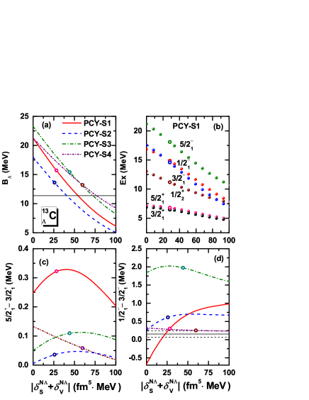
We next examine the influence of the derivative interaction terms for the other parameter sets as well. To this end, we vary $\delta^{N\Lambda}_{S}$ and $\delta^{N\Lambda}_{V}$ by keeping the values of $\alpha^{N\Lambda}_{S}$, $\alpha^{N\Lambda}_{V}$, $\alpha^{N\Lambda}_{T}$ and the ratio $\delta^{N\Lambda}_{S}/\delta^{N\Lambda}_{V}$ to be the same as the original values for each parameter set. Fig. 4(a) shows the $\Lambda$ binding energy so obtained as a function of $|\delta^{N\Lambda}_{S}+\delta^{N\Lambda}_{V}|=-(\delta^{N\Lambda}_{S}+\delta^{N\Lambda}_{V})$. The calculated $B_{\Lambda}$ with the original value of $\delta^{N\Lambda}_{S}$ and $\delta^{N\Lambda}_{V}$ is denoted by the open circle for each parameter set. $B_{\Lambda}$ decreases with increasing $|\delta^{N\Lambda}_{S}+\delta^{N\Lambda}_{V}|$ and approaches to the experimental value denoted by the thin solid line. The $\Lambda$ binding energy decreases from 21.28MeV to 15.72 MeV by adding the derivative coupling terms to the PCY-S1 interaction (that is, by changing $|\delta^{N\Lambda}_{S}+\delta^{N\Lambda}_{V}|$ from 0 to the original value denoted by the open cicle). For PCY-S2, PCY-S3, and PCY-S4 interactions, the shift is from 18.01, 23.29, and 21.27 MeV to 13.63, 15.42, and 13.22 MeV, respectively.

The excitation energies of the low-lying states as a function of the derivative coupling strength $|\delta^{N\Lambda}_{S}+\delta^{N\Lambda}_{V}|$ are shown in Figure 4(b), where $\alpha^{N\Lambda}_{S}$, $\alpha^{N\Lambda}_{V}$ , $\alpha^{N\Lambda}_{T}$ and $\delta^{N\Lambda}_{S}/\delta^{N\Lambda}_{V}$ are kept to be the same as those for PCY-S1. As one can see, the excitation energies decreases with the increase of $|\delta^{N\Lambda}_{S}+\delta^{N\Lambda}_{V}|$. Notice that the change of the $3/2^{+}$ and $5/2^{+}$ states are much smaller compared to the change in the other states. Similar behaviors are found also for the PCY-S2, PCY-S3 and PCY-S4 forces (not shown). The energy splittings of ($3/2^{+}_{1}$, $5/2^{+}_{1}$) and ($1/2^{-}_{1}$, $3/2^{-}_{1}$) states as a function of the strength of the derivative coupling terms are shown in Fig. 4(c) and (d), respectively. It is found that the $5/2^{+}_{1}$ state is always slightly higher than the $3/2^{+}_{1}$ state, which is by less than 0.15 MeV except for PCY-S1 in the range of $|\delta^{N\Lambda}_{S}+\delta^{N\Lambda}_{V}|$ shown in the figure. In contrast, the available data indicate that the $5/2^{+}_{1}$ state is slightly lower than the $3/2^{+}_{1}$ state. This discrepancy may be due to the spin-spin $N\Lambda$ interaction MCAS , which is missing in the present calculations.

For the doublet of ($1/2^{-},3/2^{-}$), the $1/2^{-}$ state is predicted to be higher than the $3/2^{-}$ state for all the forces except for the PCY-S1, with which the $1/2^{-}$ state is lower than the $3/2^{-}$ state for $|\delta^{N\Lambda}_{S}+\delta^{N\Lambda}_{V}|<17.56$ MeV. As will be discussed in the next subsection, this splitting, which reflects the spin-orbit splitting of the $p_{\Lambda}$ hyperon Mei2015 , is mainly governed by the tensor coupling term.

III.3 Effects of the tensor coupling term

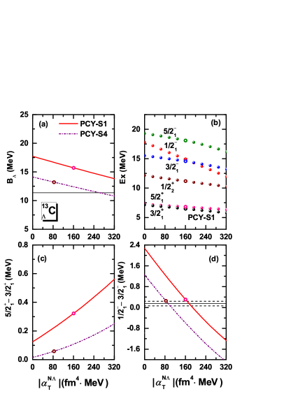
Let us next examine the effects of the tensor coupling term on hypernuclear low-lying states. For this purpose, we adopt the PCY-S1 and PCY-S4 sets of the $N\Lambda$ interaction and vary the strength $\alpha^{N\Lambda}_{T}$ for the tensor coupling term. Fig. 5(a) shows the $\Lambda$ binding energy of ${}^{13}_{~{}\Lambda}$C as a function of $|\alpha^{N\Lambda}_{T}|=-\alpha^{N\Lambda}_{T}$. The $\Lambda$ binding energy gradually decreases from 17.71 MeV (14.12 MeV) for $\alpha^{N\Lambda}_{T}=0$ to 15.72 MeV (13.22 MeV) for the original value of $\alpha^{N\Lambda}_{T}$ for the PCY-S1 (PCY-S4) force, which is indicated by the open circle in Fig. 5(a).

Figure 5(b) shows the excitation energies for the low-lying states of ${}^{13}_{~{}\Lambda}$C as a function of the tensor coupling strength $|\alpha^{N\Lambda}_{T}|$ for the PCY-S1. As already shown in the previous mean-field studies Mares94 ; Weixia14 ; Toki94 , the tensor coupling term makes the $s_{\Lambda}$ hyperon less bound by increasing the energy of the $s_{1/2}$ level. Moreover, it decreases (increases) the energy of the hyperon $p_{3/2}$ ($p_{1/2}$) state. This is consistent with Fig.5(a) for the ground state ($1/2^{+}$) of the ${}^{13}_{~{}\Lambda}$C, the energy of which decreases by the tensor coupling. As a result, the $\Lambda$ binding energy is reduced by 0.9 MeV for the PCY-S1 and 1.99 MeV for the PCY-S4 after turning on the tensor coupling term. At the same time, the tensor coupling term decreases (increases) the energy of the $3/2^{-}$ ($1/2^{-}$) state, which mainly consists of the $p_{3/2}$ ($p_{1/2}$) hyperon coupled to the ground state ($0^{+}$) of ¹²C. Since the $1/2^{-}$ changes more significantly than the $3/2^{-}$ state, the higher lying $1/2^{-}$ state approaches the $3/2^{-}$ state and even becomes lower than the $3/2^{-}$ state for large values of the tensor coupling strength, indicating that the energy splitting of the $1/2^{-}$ and $3/2^{-}$ states is sensitive to the tensor coupling strength. For the PCY-S1 and PCY-S4 forces, the energy difference between $1/2^{-}_{1}$ and $3/2^{-}_{1}$ states decreases from 2.28 MeV to 0.31 MeV, and from 1.25 MeV to 0.25 MeV, respectively, while turning on the tensor coupling term. For the energy gap between the $3/2^{+}_{1}$ and $5/2^{+}_{1}$ states, it increases with increasing the $|\alpha^{N\Lambda}_{T}|$, as shown in Fig.5(c). Again, the tensor coupling term does not invert the energy ordering of the $3/2^{+}_{1}$ and $5/2^{+}_{1}$ states.

IV Summary

We have implemented the higher-order derivative and the tensor terms in the point coupling $N\Lambda$ interaction in the microscopic particle-rotor model for hypernuclear low-lying states. By taking ${}^{13}_{~{}\Lambda}$C as an example, we have adopted the four sets of effective $N\Lambda$ interaction, which were adjusted at the mean-field level to the $\Lambda$ binding energy. We have shown that the four parameter sets yield a qualitatively similar low-lying spectrum to one another, even though these parameter sets were obtained using only the ground state energy.

We have discussed in detail the impact of each $N\Lambda$ interaction term on hypernuclear low-lying states for ${}^{13}_{~{}\Lambda}$C. We have shown that both the second-order derivative and the tensor coupling terms raise the energy of hypernuclear states and thus reduce the $\Lambda$ binding energy. With the increase of the tensor coupling strength, the excitation energy of the $1/2^{-}$ state has been found to decrease faster than the $3/2^{-}$ states. As a result, the energy difference $E(1/2^{-})-E(3/2^{-})$ decreases to a small value and even changes its sign for large values of the tensor coupling term. We have also found that the energy ordering of the $3/2^{+}_{1}$ and $5/2^{+}_{1}$ states cannot be reproduced by the present effective $N\Lambda$ interaction. We note that the four-fermion coupling terms $(\bar{\psi}_{N}\Gamma_{i}\psi_{N})(\bar{\psi}_{\Lambda}\Gamma_{i}\psi_{\Lambda})$ with $\Gamma_{i}=\sigma_{\mu\nu}$ and $\gamma_{\mu}\gamma^{5}$, which provides the spin-spin $N\Lambda$ interaction Polinder06 , are not taken into account in the present study. This interaction term may have an important influence on the energy ordering of the $3/2^{+}_{1}$ and $5/2^{+}_{1}$ states. It will be interesting to study in near future the role of these terms in hypernuclear spectroscopy with the present microscopic particle-rotor model.

Another interesting work is to compare directly between the microscopic particle-rotor model and the generator coordinate method for the whole $\Lambda$ hypernuclei Mei15-2 using the same point-coupling $N\Lambda$ interaction. A work is now in progress, and we will report on it in a separate paper.

Appendix A: The $N\Lambda$ effective interaction and the corresponding energy functional

In this Appendix A, we show that the $N\Lambda$ interaction given by Eqs. (II), (II) and (10) lead to the energy functional given by Eq.(II). The energy functional for $N\Lambda$ interaction is given by the expectation value of the effective interaction $\hat{V}^{N\Lambda}$ at the Hartree level,

$$E^{N\Lambda}_{\rm int}=\sum_{i=1}^{A_{c}}\int d\mbox{\boldmath$r$}d\mbox{\boldmath$r$}^{\prime}\psi^{\dagger}_{\Lambda}(\mbox{\boldmath$r$})\psi^{\dagger}_{i}(\mbox{\boldmath$r$}^{\prime})\hat{V}^{N\Lambda}(\mbox{\boldmath$r$},\mbox{\boldmath$r$}^{\prime})\psi_{\Lambda}(\mbox{\boldmath$r$})\psi_{i}(\mbox{\boldmath$r$}^{\prime}).$$ (18)

Substituting the LO scalar effective interaction term,

$$\hat{V}^{N\Lambda}_{S}(\mbox{\boldmath$r$},\mbox{\boldmath$r$}^{\prime})=\alpha_{S}^{N\Lambda}\gamma^{0}_{\Lambda}\delta(\mbox{\boldmath$r$}-\mbox{\boldmath$r$}^{\prime})\gamma^{0}_{N}$$ (19)

to Eq.(18), one finds

$$E^{N\Lambda}_{\rm S}$$

$$=\sum_{i=1}^{A_{c}}\int d\mbox{\boldmath$r$}d\mbox{\boldmath$r$}^{\prime}\psi^{\dagger}_{\Lambda}(\mbox{\boldmath$r$})\psi^{\dagger}_{i}(\mbox{\boldmath$r$}^{\prime})\alpha_{S}^{N\Lambda}\gamma^{0}_{\Lambda}\delta(\mbox{\boldmath$r$}-\mbox{\boldmath$r$}^{\prime})\gamma^{0}_{N}\psi_{\Lambda}(\mbox{\boldmath$r$})\psi_{i}(\mbox{\boldmath$r$}^{\prime})$$

$$=\alpha_{S}^{N\Lambda}\sum_{i=1}^{A_{c}}\int d\mbox{\boldmath$r$}\psi^{\dagger}_{\Lambda}(\mbox{\boldmath$r$})\gamma^{0}_{\Lambda}\psi_{\Lambda}(\mbox{\boldmath$r$})\psi^{\dagger}_{i}(\mbox{\boldmath$r$})\gamma^{0}_{N}\psi_{i}(\mbox{\boldmath$r$})$$

$$=\int d\mbox{\boldmath$r$}\alpha_{S}^{N\Lambda}\rho^{\Lambda}_{S}(\mbox{\boldmath$r$})\rho_{S}(\mbox{\boldmath$r$}),$$ (20)

where $\rho_{S}$ and $\rho^{\Lambda}_{S}$ are the scalar densities defined as

$$\rho_{S}(\mbox{\boldmath$r$})=\sum_{i=1}^{A_{c}}\bar{\psi}_{i}(\mbox{\boldmath$r$})\psi_{i}(\mbox{\boldmath$r$}),~{}~{}\rho^{\Lambda}_{S}(\mbox{\boldmath$r$})=\bar{\psi}_{\Lambda}(\mbox{\boldmath$r$})\psi_{\Lambda}(\mbox{\boldmath$r$}).$$ (21)

The effective interaction with the scalar derivative term,

$$\hat{V}^{N\Lambda}_{\rm Der}(\mbox{\boldmath$r$},\mbox{\boldmath$r$}^{\prime})= \delta_{S}^{N\Lambda}\gamma^{0}_{\Lambda}\Big{[}\overleftarrow{\nabla}^{2}\delta(\mbox{\boldmath$r$}-\mbox{\boldmath$r$}^{\prime})+\delta(\mbox{\boldmath$r$}-\mbox{\boldmath$r$}^{\prime})\overrightarrow{\nabla}^{2}$$

$$+2\overleftarrow{\nabla}\cdot\delta(\mbox{\boldmath$r$}-\mbox{\boldmath$r$}^{\prime})\overrightarrow{\nabla}\Big{]}\gamma^{0}_{N},$$ (22)

leads to

$$E^{N\Lambda}_{\rm S}$$

$$=\sum_{i=1}^{A_{c}}\int d\mbox{\boldmath$r$}d\mbox{\boldmath$r$}^{\prime}\psi^{\dagger}_{\Lambda}(\mbox{\boldmath$r$})\psi^{\dagger}_{i}(\mbox{\boldmath$r$}^{\prime})\delta_{S}^{N\Lambda}\gamma^{0}_{\Lambda}\Big{[}\overleftarrow{\nabla}^{2}\delta(\mbox{\boldmath$r$}-\mbox{\boldmath$r$}^{\prime})$$

$$~{}~{}~{}+\delta(\mbox{\boldmath$r$}-\mbox{\boldmath$r$}^{\prime})\overrightarrow{\nabla}^{2}+2\overleftarrow{\nabla}\cdot\delta(\mbox{\boldmath$r$}-\mbox{\boldmath$r$}^{\prime})\overrightarrow{\nabla}\Big{]}\gamma^{0}_{N}\psi_{\Lambda}(\mbox{\boldmath$r$})\psi_{i}(\mbox{\boldmath$r$}^{\prime})$$

$$=\delta_{S}^{N\Lambda}\sum_{i=1}^{A_{c}}\int d\mbox{\boldmath$r$}\Big{\{}[\nabla^{2}\psi^{\dagger}_{\Lambda}(\mbox{\boldmath$r$})\gamma^{0}_{\Lambda}]\psi_{\Lambda}(\mbox{\boldmath$r$})+[\psi^{\dagger}_{\Lambda}(\mbox{\boldmath$r$})\gamma^{0}_{\Lambda}][\nabla^{2}\psi_{\Lambda}(\mbox{\boldmath$r$})]$$

$$~{}~{}~{}+2[\nabla\psi^{\dagger}_{\Lambda}(\mbox{\boldmath$r$})\gamma^{0}_{\Lambda}]\cdot[\nabla\psi_{\Lambda}(\mbox{\boldmath$r$})]\Big{\}}[\psi^{\dagger}_{i}(\mbox{\boldmath$r$})\gamma^{0}_{N}\psi_{i}(\mbox{\boldmath$r$})]$$

$$=\int d\mbox{\boldmath$r$}\delta_{S}^{N\Lambda}\rho_{S}(\mbox{\boldmath$r$})\nabla^{2}\rho^{\Lambda}_{S}(\mbox{\boldmath$r$}).$$ (23)

A similar derivation holds also for the vector part of the $N\Lambda$ interaction.

On the other hand, the tensor effective interaction,

$$\hat{V}^{N\Lambda}_{T}(\mbox{\boldmath$r$},\mbox{\boldmath$r$}^{\prime})=i\alpha_{T}^{N\Lambda}\Big{[}\overleftarrow{\nabla}\cdot\mbox{\boldmath$\gamma$}\delta(\mbox{\boldmath$r$}-\mbox{\boldmath$r$}^{\prime})+\delta(\mbox{\boldmath$r$}-\mbox{\boldmath$r$}^{\prime})\overrightarrow{\nabla}\cdot\mbox{\boldmath$\gamma$}\Big{]}$$ (24)

leads to

$$E^{N\Lambda}_{\rm T}$$

$$=\sum_{i=1}^{A_{c}}\int d\mbox{\boldmath$r$}d\mbox{\boldmath$r$}^{\prime}\psi^{\dagger}_{\Lambda}(\mbox{\boldmath$r$})\psi^{\dagger}_{i}(\mbox{\boldmath$r$}^{\prime})i\alpha_{T}^{N\Lambda}\Big{[}\overleftarrow{\nabla}\cdot\mbox{\boldmath$\gamma$}\delta(\mbox{\boldmath$r$}-\mbox{\boldmath$r$}^{\prime})$$

$$~{}~{}~{}+\delta(\mbox{\boldmath$r$}-\mbox{\boldmath$r$}^{\prime})\overrightarrow{\nabla}\cdot\mbox{\boldmath$\gamma$}\Big{]}\psi_{\Lambda}(\mbox{\boldmath$r$})\psi_{i}(\mbox{\boldmath$r$}^{\prime})$$

$$=\alpha_{T}^{N\Lambda}\sum_{i=1}^{A_{c}}\int d\mbox{\boldmath$r$}\Big{\{}[\nabla\psi^{\dagger}_{\Lambda}(\mbox{\boldmath$r$})\gamma^{0}_{\Lambda}]\cdot i\mbox{\boldmath$\alpha$}\psi_{\Lambda}(\mbox{\boldmath$r$})$$

$$~{}~{}~{}+[\psi^{\dagger}_{\Lambda}(\mbox{\boldmath$r$})\gamma^{0}_{\Lambda}][\nabla\cdot i\mbox{\boldmath$\alpha$}\psi_{\Lambda}(\mbox{\boldmath$r$})]\Big{\}}[\psi^{\dagger}_{i}(\mbox{\boldmath$r$})\psi_{i}(\mbox{\boldmath$r$})]$$

$$=\int d\mbox{\boldmath$r$}\alpha_{T}^{N\Lambda}\rho_{V}(\mbox{\boldmath$r$})[\nabla\cdot(\bar{\psi}_{\Lambda}(\mbox{\boldmath$r$})i\mbox{\boldmath$\alpha$}\psi_{\Lambda}(\mbox{\boldmath$r$}))]$$

$$=\int d\mbox{\boldmath$r$}\alpha_{T}^{N\Lambda}\rho_{V}(\mbox{\boldmath$r$})\rho^{\Lambda}_{T}(\mbox{\boldmath$r$}),$$ (25)

where $\rho_{V}$ and $\rho^{\Lambda}_{T}$ are the vector and the tensor densities defined as

$$\rho_{V}(\mbox{\boldmath$r$})= \sum_{i=1}^{A_{c}}\psi^{\dagger}_{i}(\mbox{\boldmath$r$})\psi_{i}(\mbox{\boldmath$r$}),$$ (26a)

$$\rho^{\Lambda}_{T}(\mbox{\boldmath$r$})= \nabla\cdot(\bar{\psi}_{\Lambda}(\mbox{\boldmath$r$})i\mbox{\boldmath$\alpha$}\psi_{\Lambda}(\mbox{\boldmath$r$})).$$ (26b)

Putting all these together, we finally obtain Eq.(II).

Appendix B: A derivation of Eq.(16) for the matrix elements of the vector derivative coupling term

With the $N\Lambda$ vector derivative effective interaction $\displaystyle\hat{V}_{D}=\delta_{V}^{N\Lambda}\Big{[}\overleftarrow{\nabla}^{2}\delta(\mbox{\boldmath$r$}-\mbox{\boldmath$r$}_{i})+\delta(\mbox{\boldmath$r$}-\mbox{\boldmath$r$}_{i})\overrightarrow{\nabla}^{2}+2\overleftarrow{\nabla}\cdot\delta(\mbox{\boldmath$r$}-\mbox{\boldmath$r$}_{i})\overrightarrow{\nabla}\Big{]}$, and the definition of

$${\mathscr{F}}^{JM}_{jlI}(\hat{\mbox{\boldmath$r$}},\{\mbox{\boldmath$r$}_{i}\})=\sum_{m_{I}m}C^{JM}_{Im_{I}jm}{\mathscr{Y}}_{jlm}(\hat{\mbox{\boldmath$r$}})\Phi_{Im_{I}}(\{\mbox{\boldmath$r$}_{i}\}),$$ (27)

where ${\mathscr{Y}}_{jlm}(\hat{{\mbox{\boldmath$r$}}})$ is the spinor spherical harmonics,

$${\mathscr{Y}}_{j\ell m}(\hat{\mbox{\boldmath$r$}})=\sum_{m_{l}m_{s}}C^{jm}_{lm_{l}\frac{1}{2}m_{s}}Y_{lm_{l}}(\vartheta,\varphi)\chi_{m_{s}},$$ (28)

the coupling matrix element of the vector derivative term reads

$$\langle R^{k}_{\alpha l}(r){\mathscr{F}}^{JM}_{jlI}(\hat{\mbox{\boldmath$r$}},\{\mbox{\boldmath$r$}_{i}\})|\hat{V}_{D}|{\mathscr{F}}^{JM}_{j^{\prime}l^{\prime}I^{\prime}}(\hat{\mbox{\boldmath$r$}},\{\mbox{\boldmath$r$}_{i}\})R^{k^{\prime}}_{\alpha^{\prime}l^{\prime}}(r)\rangle$$

$$= \delta_{S}^{N\Lambda}\sum_{m_{I}m}\sum_{m^{\prime}_{I}m^{\prime}}C^{JM}_{Im_{I}jm}C^{JM}_{I^{\prime}m^{\prime}_{I}j^{\prime}m^{\prime}}$$

$$\times\sum_{\lambda\mu}\int r^{2}dr\int d\hat{\mbox{\boldmath$r$}}\langle\Phi_{Im_{I}}|\sum_{i=1}^{A_{c}}\frac{\delta(r-r_{i})}{rr_{i}}Y_{\lambda\mu}(\hat{\mbox{\boldmath$r$}}_{i})|\Phi_{I^{\prime}m^{\prime}_{I}}\rangle$$

$$\times Y_{\lambda\mu}^{*}(\hat{\mbox{\boldmath$r$}})\Delta[{\mathscr{Y}}_{j\ell m}^{*}(\hat{\mbox{\boldmath$r$}}){\mathscr{Y}}_{j^{\prime}\ell^{\prime}m^{\prime}}(\hat{\mbox{\boldmath$r$}})R^{k}_{\alpha l}(r)R^{k^{\prime}}_{\alpha^{\prime}l^{\prime}}(r)].$$ (29)

Here, we notice

$$\langle\Phi_{Im_{I}}|\sum^{A_{c}}_{i=1}\frac{\delta(r-r_{i})}{rr_{i}}Y_{\lambda\mu}(\hat{\mbox{\boldmath$r$}}_{i})|\Phi_{I^{\prime}m^{\prime}_{I}}\rangle$$

$$= (-1)^{I-m_{I}}\left(\begin{matrix}I&\lambda&I^{\prime}\\ -m_{I}&\mu&m^{\prime}_{I}\end{matrix}\right)\langle\Phi_{I}||\sum^{A_{c}}_{i=1}\frac{\delta(r-r_{i})}{rr_{i}}Y_{\lambda}(\hat{\mbox{\boldmath$r$}}_{i})|\Phi_{I^{\prime}}\rangle$$

$$= (-1)^{I-m_{I}}\left(\begin{matrix}I&\lambda&I^{\prime}\\ -m_{I}&\mu&m^{\prime}_{I}\end{matrix}\right)\rho^{II^{\prime}}_{\lambda,V}(r).$$ (30)

With the relation of

$${\mathscr{Y}}_{j\ell m}^{*}(\hat{\mbox{\boldmath$r$}}){\mathscr{Y}}_{j^{\prime}\ell^{\prime}m^{\prime}}(\hat{\mbox{\boldmath$r$}})$$

$$= \sum_{m_{l}m_{s}}\sum_{m^{\prime}_{l}m^{\prime}_{s}}C^{jm}_{lm_{l}\frac{1}{2}m_{s}}C^{j^{\prime}m^{\prime}}_{l^{\prime}m^{\prime}_{l}\frac{1}{2}m^{\prime}_{s}}\delta_{m_{s}m^{\prime}_{s}}(-1)^{m_{l}}$$

$$\times\sum_{LM}\frac{\hat{l}\hat{l}^{\prime}}{\sqrt{4\pi}\hat{L}}C^{L0}_{l0l^{\prime}0}C^{LM}_{l-m_{l}l^{\prime}m^{\prime}_{l}}Y_{Lm_{L}}(\hat{\mbox{\boldmath$r$}}),$$ (31)

we have

$$\Delta[{\mathscr{Y}}_{j\ell m}^{*}(\hat{\mbox{\boldmath$r$}}){\mathscr{Y}}_{j^{\prime}\ell^{\prime}m^{\prime}}(\hat{\mbox{\boldmath$r$}})]$$

$$=\sum_{m_{l}m_{s}}\sum_{m^{\prime}_{l}m^{\prime}_{s}}\sum_{LM}\frac{\hat{l}\hat{l}^{\prime}}{\sqrt{4\pi}\hat{L}}C^{jm}_{lm_{l}\frac{1}{2}m_{s}}C^{j^{\prime}m^{\prime}}_{l^{\prime}m^{\prime}_{l}\frac{1}{2}m^{\prime}_{s}}\delta_{m_{s}m^{\prime}_{s}}(-1)^{m_{l}}$$

$$\times C^{L0}_{l0l^{\prime}0}C^{LM}_{l-m_{l}l^{\prime}m^{\prime}_{l}}\left[\frac{1}{r^{2}}\frac{d}{dr}\left(r^{2}\frac{d}{dr}\right)-\frac{L(L+1)}{r^{2}}\right]Y_{Lm_{L}}(\hat{\mbox{\boldmath$r$}}).$$ (32)

According to the orthogonalization of the spherical harmonics,

$$\int Y_{\lambda\mu}^{*}(\hat{\mbox{\boldmath$r$}})Y_{Lm_{L}}(\hat{\mbox{\boldmath$r$}})d\hat{\mbox{\boldmath$r$}}=\delta_{\lambda,L}\delta_{\mu,m_{L}},$$ (33)

the matrix element is then given by

$$\langle R^{k}_{\alpha l}(r){\mathscr{F}}^{JM}_{jlI}(\hat{\mbox{\boldmath$r$}},\{\mbox{\boldmath$r$}_{i}\})|\hat{V}_{D}|{\mathscr{F}}^{JM}_{j^{\prime}l^{\prime}I^{\prime}}(\hat{\mbox{\boldmath$r$}},\{\mbox{\boldmath$r$}_{i}\})R^{k^{\prime}}_{\alpha^{\prime}l^{\prime}}(r)\rangle$$

$$= \delta_{V}^{N\Lambda}(-1)^{j^{\prime}+I+J}\sum_{\lambda}\left\{\begin{matrix}J&I&l\\ \lambda&j^{\prime}&I^{\prime}\end{matrix}\right\}\langle j\ell||Y_{\lambda}||j^{\prime}\ell^{\prime}\rangle$$

$$~{}\times\int r^{2}dr\rho^{II^{\prime}}_{\lambda,V}(r)\left[\frac{1}{r^{2}}\frac{d}{dr}\left(r^{2}\frac{d}{dr}\right)-\frac{\lambda(\lambda+1)}{r^{2}}\right]$$

$$~{}\times[R^{k}_{\alpha l}(r)R^{k^{\prime}}_{\alpha^{\prime}l^{\prime}}(r)].$$ (34)

Appendix C: A derivation of Eq.(16f) for the matrix elements of the tensor coupling term

The matrix elements of the tensor coupling term is given by

$$T_{\alpha\alpha^{\prime}}^{kk^{\prime}} \equiv\langle R^{k}_{\alpha l}(r){\mathscr{F}}^{JM}_{jlI}(\hat{\mbox{\boldmath$r$}},\{\mbox{\boldmath$r$}_{i}\})|\alpha_{T}^{N\Lambda}\sum_{i=1}^{A_{c}}\Big{[}\overleftarrow{\nabla}\delta(\mbox{\boldmath$r$}-\mbox{\boldmath$r$}_{i})$$

$$~{}+\delta(\mbox{\boldmath$r$}-\mbox{\boldmath$r$}_{i})\overrightarrow{\nabla}\Big{]}\cdot\mbox{\boldmath$\sigma$}|{\mathscr{F}}^{JM}_{j^{\prime}\tilde{l}^{\prime}I^{\prime}}(\hat{\mbox{\boldmath$r$}},\{\mbox{\boldmath$r$}_{i}\})R^{k^{\prime}}_{\alpha^{\prime}\tilde{l}^{\prime}}(r)\rangle$$

$$=\alpha^{N\Lambda}_{T}\sum_{m^{\prime}_{I}m^{\prime}}\sum_{m_{I}m}C^{JM}_{I^{\prime}m^{\prime}_{I}j^{\prime}m^{\prime}}C^{JM}_{Im_{I}jm}$$

$$~{}\times\sum_{\lambda\mu}\int r^{2}drd\hat{\mbox{\boldmath$r$}}\langle\Phi_{Im_{I}}|\sum_{i}^{A_{c}}\frac{\delta(r-r_{i})}{rr_{i}}Y_{\lambda\mu}(\hat{\mbox{\boldmath$r$}}_{i})|\Phi_{I^{\prime}m^{\prime}_{I}}\rangle$$

$$~{}\times Y_{\lambda\mu}^{*}(\hat{\mbox{\boldmath$r$}})\nabla\cdot[R^{k*}_{\alpha l}(r){\mathscr{Y}}^{*}_{jlm}(\hat{\mbox{\boldmath$r$}})\mbox{\boldmath$\sigma$}R^{k^{\prime}}_{\alpha^{\prime}\tilde{l}^{\prime}}(r){\mathscr{Y}}_{j^{\prime}\tilde{l}^{\prime}m^{\prime}}(\hat{\mbox{\boldmath$r$}})].$$ (35)

Notice

$$\nabla\cdot[R^{k*}_{\alpha l}(r){\mathscr{Y}}^{*}_{jlm}(\hat{\mbox{\boldmath$r$}})\mbox{\boldmath$\sigma$}R^{k^{\prime}}_{\alpha^{\prime}\tilde{l}^{\prime}}(r){\mathscr{Y}}_{j^{\prime}\tilde{l}^{\prime}m^{\prime}}(\hat{\mbox{\boldmath$r$}})]$$

$$=\Big{[}-\frac{dR^{k}_{\alpha l}(r)}{dr}-\frac{\kappa+1}{r}R^{k}_{\alpha l}(r)\Big{]}[R^{k^{\prime}}_{\alpha^{\prime}\tilde{l}^{\prime}}(r){\mathscr{Y}}^{*}_{j\tilde{l}m}(\hat{\mbox{\boldmath$r$}}){\mathscr{Y}}_{j^{\prime}\tilde{l}^{\prime}m^{\prime}}(\hat{\mbox{\boldmath$r$}})]$$

$$-\Big{[}\frac{dR^{k^{\prime}}_{\alpha^{\prime}\tilde{l}^{\prime}}(r)}{dr}-\frac{\kappa^{\prime}-1}{r}R^{k^{\prime}}_{\alpha^{\prime}\tilde{l}^{\prime}}(r)\Big{]}[R^{k*}_{\alpha l}(r){\mathscr{Y}}^{*}_{jlm}(\hat{\mbox{\boldmath$r$}}){\mathscr{Y}}_{j^{\prime}l^{\prime}m^{\prime}}(\hat{\mbox{\boldmath$r$}})].$$ (36)

With the Wigner-Eckart theroem, one obtains

$$\int d\hat{\mbox{\boldmath$r$}}{\mathscr{Y}}^{*}_{jlm}(\hat{\mbox{\boldmath$r$}})Y_{\lambda\mu}^{*}(\hat{\mbox{\boldmath$r$}}){\mathscr{Y}}_{j^{\prime}l^{\prime}m^{\prime}}(\hat{\mbox{\boldmath$r$}})$$

$$=(-1)^{\mu+j-m}\left(\begin{matrix}j&\lambda&j^{\prime}\\ -m&-\mu&m^{\prime}\end{matrix}\right)\langle jl||Y_{\lambda}||j^{\prime}l^{\prime}\rangle.$$ (37)

From the relation

$$\sum_{m^{\prime}_{I}m^{\prime}}\sum_{m_{I}m}\sum_{\mu}C^{JM}_{I^{\prime}m^{\prime}_{I}j^{\prime}m^{\prime}}C^{JM}_{Im_{I}jm}(-1)^{I-m_{I}}\left(\begin{matrix}I&\lambda&I^{\prime}\\ -m_{I}&\mu&m^{\prime}_{I}\end{matrix}\right)$$

$$\times(-1)^{\mu+j-m}\left(\begin{matrix}j&\lambda&j^{\prime}\\ -m&-\mu&m^{\prime}\end{matrix}\right)=(-1)^{I^{\prime}+J+j}\left\{\begin{matrix}J&I&j\\ \lambda&j^{\prime}&I^{\prime}\end{matrix}\right\},$$ (38)

one finally obtains

$$T_{\alpha\alpha^{\prime}}^{kk^{\prime}} =-\alpha^{N\Lambda}_{T}(-1)^{j+I^{\prime}+J}\sum_{\lambda}\left\{\begin{matrix}J&I&j\\ \lambda&j^{\prime}&I^{\prime}\end{matrix}\right\}\int r^{2}dr\rho^{I^{\prime}I}_{\lambda,V}(r)$$

$$~{}\times\Big{\{}\Big{[}\frac{dR^{k}_{\alpha l}(r)}{dr}+\frac{\kappa+1}{r}R^{k}_{\alpha l}(r)\Big{]}R^{k^{\prime}}_{\alpha^{\prime}\tilde{l}^{\prime}}(r)\langle j\tilde{l}||Y_{\lambda}||j^{\prime}\tilde{l}^{\prime}\rangle$$

$$~{}+\Big{[}\frac{dR^{k^{\prime}}_{\alpha^{\prime}\tilde{l}^{\prime}}(r)}{dr}-\frac{\kappa^{\prime}-1}{r}R^{k^{\prime}}_{\alpha^{\prime}\tilde{l}^{\prime}}(r)\Big{]}R^{k}_{\alpha l}(r)\langle jl||Y_{\lambda}||j^{\prime}l^{\prime}\rangle\Big{\}}.$$ (39)

References

• (1) O. Hashimoto and H. Tamura, Prog. Part. Nucl. Phys. 57, 564 (2006).
• (2) H. Tamura, Int. J. Mod. Phys. A 24, 2101 (2009).
• (3) N. Glendenning, Compact Stars (Springer-Verlag, New York, 2000).
• (4) R. Wirth, D. Gazda, P. Navratil, A. Calic, J. Langhammer, and R. Roth, Phys. Rev. Lett. 113, 192502 (2014).
• (5) T. Motoba, H. Bandō, and K. Ikeda, Prog. Theor. Phys. 70, 189 (1983).
• (6) E. Hiyama, M. Kamimura, K. Miyazaki, and T. Motoba, Phys. Rev. C 59, 2351 (1999).
• (7) H. Bando, T. Motoba and J. Žofka, Int. J. Mod. Phys. A 5, 4021 (1990).
• (8) E. Hiyama, Y. Kino, and M. Kamimura, Prog. Part. Nucl. Phys. 51, 223 (2003).
• (9) E. Cravo, A. C. Fonseca, Y. Koike, Phys. Rev. C 66, 014001 (2002).
• (10) V. M. Suslov, I. Filikhin, and B. Vlahovic, J. Phys. G: Nucl. Part. Phys. 30, 513 (2004).
• (11) M. Shoeb and Sonika, Phys. Rev. C 79, 054321 (2009).
• (12) R. H. Dalitz and A. Gal, Ann. Phys. (N.Y.) 116, 167 (1978).
• (13) A. Gal, J.M. Soper, and R.H. Dalitz, Ann. Phys. (N.Y.) 63, 53 (1971).
• (14) D. J. Millener, Nucl. Phys. A804, 84 (2008); A914, 109 (2013).
• (15) M. Isaka, M. Kimura, A. Doté and A. Ohnishi, Phys. Rev. C 83, 044323 (2011).
• (16) M. Isaka, M. Kimura, A. Doté and A. Ohnishi, Phys. Rev. C 83, 054304 (2011).
• (17) M. Isaka, H. Homma, M. Kimura, A. Doté and A. Ohnishi, Phys. Rev. C 85, 034303 (2012).
• (18) M. Isaka, M. Kimura, A. Doté and A. Ohnishi, Phys. Rev. C 87, 021304(R) (2013).
• (19) X. R. Zhou , H.-J. Schulze, H. Sagawa, C. X. Wu, and E.-G. Zhao, Phys. Rev. C 76, 034312 (2007).
• (20) M. T. Win and K. Hagino, Phys. Rev. C 78, 054311 (2008).
• (21) H.-J. Schulze, M. T. Win, K. Hagino, and H. S. Sagawa, Prog. Theo. Phys. 123, 569 (2010).
• (22) Myaing Thi Win, K. Hagino, and T. Koike, Phys. Rev. C 83, 014301 (2011).
• (23) B.-N. Lu, E.-G. Zhao, and S.-G. Zhou, Phys. Rev. C 84, 014328 (2011).
• (24) W. X. Xue, J. M. Yao, K. Hagino, Z. P. Li, H. Mei, and Y. Tanimura, Phys. Rev. C 91, 024327 (2015).
• (25) A. Li, E. Hiyama, X.-R. Zhou, and H. Sagawa, Phys. Rev. C 87, 014333 (2013).
• (26) B.-N. Lu, E. Hiyama, H. Sagawa, and S.-G. Zhou, Phys. Rev. C 89, 044307 (2014).
• (27) K. Hagino and J.M. Yao, in Relativistic Density Functional for Nuclear Structure, Int. Rev. Nucl. Phys. 10, 263-303 (2016), edited by J. Meng (World Scientific, Singapore, 2016).
• (28) H. Mei, K. Hagino, and J. M. Yao, Phys. Rev. C 93, 011301(R) (2016).
• (29) H. Mei, K. Hagino, J. M. Yao, and T. Motoba, Phys. Rev. C 90, 064302 (2014).
• (30) H. Mei, K. Hagino, J. M. Yao, and T. Motoba, Phys. Rev. C 91, 064305 (2015).
• (31) Y. Tanimura and K. Hagino, Phys. Rev. C 85, 014306 (2012).
• (32) E. Hiyama, Y. Funaki, N. Kaiser, and W. Weise, Prog. Theor. Exp. Phys., 2014, 013D01(2014).
• (33) J. V.Noble, Phys. Lett. B 89, 325,(1980).
• (34) T. Burvenich, D. G. Madland, J. A. Maruhn, and P.-G. Reinhard, Phys. Rev. C 65, 044308 (2002).
• (35) P. Ring and P. Schuck, The Nuclear Many-Body Problem (Springer-Verlag, Berlin, 1980).
• (36) H. Polinder, J. Haidenbauer, Ulf-G. Meissner, Nucl. Phys. A779, 244 (2006).
• (37) J. M. Yao, M. Bender, and P.-H. Heenen, Phys. Rev. C 91, 024301 (2015).
• (38) S. Ajimura et al., Phys, Rev. Lett. 86,4255 (2001).
• (39) H. Kohri et al., Phys.Rev.C 65,034607 (2002).
• (40) Y. Sugahara, and H. Toki, Prog. Theo. Phys. 92, 803(1994).
• (41) L. Canton, K. Amos, S. Karataglidis, and J. P. Svenne, Int. J. Mod. Phys. E 19, 1435 (2010).
• (42) J. Mare$\check{\mathrm{s}}$ and B. K. Jenings, Phys. Rev. C 49, 2472-2478 (1994).