Entangled Bloch spheres: Bloch matrix and two-qubit state space

Abstract

We represent a two-qubit density matrix in the basis of Pauli matrix tensor products, with the coefficients constituting a Bloch matrix, analogous to the single qubit Bloch vector. We find the quantum state positivity requirements on the Bloch matrix components, leading to three important inequalities, allowing us to parametrize and visualize the two-qubit state space. Applying the singular value decomposition naturally separates the degrees of freedom to local anr nonlocal, and simplifies the positivity inequalities. It also allows us to geometrically represent a state as two entangled Bloch spheres with superimposed correlation axes. It is shown that unitary transformations, local or nonlocal, have simple interpretations as axis rotations or mixing of certain degrees of freedom. The nonlocal unitary invariants of the state are then derived in terms of local unitary invariants. The positive partial transpose criterion for entanglement is generalized, and interpreted as a reflection, or a change of a single sign. The formalism is used to characterize maximally entangled states, and generalize two-qubit isotropic and Werner states.

PACS numbers

03.65.Ud, 03.67.Mn, 03.67.Bg, 03.67.Lx.

I Introduction

Probabilistic mixtures of single qubit quantum states can be represented by a density matrix (von Neumann, 1927). The density matrix may be written in the Pauli Matrix basis, with the coefficients making up the Bloch vector (Bloch, 1946). The latter has the simple geometry of a vector inside a unit Bloch sphere, whose magnitude indicates the state’s purity, and whose rotations are unitary transformations.

The simplicity of this representation motivated many authors to generalize it to quantum systems of higher dimensions. In three dimensions, the basis of Gell-Mann matrices (Gell-Mann and Ne’eman, 1964) led to an irregularly shaped Bloch vector space (Kimura, 2003; Kimura and Kossakowski, 2005; Byrd and Khaneja, 2003). Generalized Gell-Mann matrices have been used as the basis in the four-dimensional (two-qubit) case (Jakóbczyk and Siennicki, 2001; Tilma et al., 2002; Bertlmann and Krammer, 2008), again leading to a space without much symmetry. Two-qubit state space has also been analyzed through Hopf fibrations (Mosseri and Dandoloff, 2001), and steering ellipsoids (Jevtic et al., 2014; Milne et al., 2014).

In this work, we make use of tensor products of Pauli matrices as our four-dimensional system basis, with the coefficients representing entries of a Bloch matrix. Numerous authors have use a similar approach (Horodecki et al., 1995; Horodecki and Horodecki, 1996; Linden et al., 1999; Makhlin, 2002; Barrett, 2002; Kuś and Zyczkowski, 2001; Abouraddy et al., 2002; Spengler et al., 2011; Jevtic et al., 2014; Milne et al., 2014; Aerts and de Bianchi, 2015; James et al., 2001; Kagalwala et al., 2015; Rajagopal and Rendell, 2001). We go further by studying the properties of this representation, and in particular, deriving the positivity conditions.

The positivity of the quantum states leads to three inequalities that allow us to parametrize and visualize the state space. The inequalities suggest a singular value decomposition, which simplifies the positivity conditions and reproduces known unitary invariants (Makhlin, 2002) with additional insights. The conditions also allow us to generalize the positive partial transpose criterion for entanglement (Peres, 1996; Horodecki et al., 1996), and strikingly interpret it as a reflection, or a change of a single sign. We also find that the most basic nonlocal transformations (Zhang et al., 2003) reduce to a family of two-dimensional rotation matrices which mix various degrees of freedom of the Bloch matrix representation.

The paper is organized as follows; Secs. II and III review the Bloch vector representation, with the former on qubits and qutrits, and the latter on two-qubit systems. The positivity inequalities, a key result of this paper, are derived in Sec. IV. The singular value decomposition, along with its simplification of the positivity conditions and representation of a quantum state as a pair of entangled Bloch spheres are presented in Sec. V. The actions of unitary operations, local and nonlocal, and their invariants are expressed in the Bloch representation in Sec. VI. Section VII provides a novel geometric interpretation and generalization of the positive partial transpose entanglement criterion. Section VIII applies the formalism to the characterization of maximally entangled, pure states, and generalized isotropic/Werner states. Geometric visualization of the quantum state space, indicating separability and entanglement, takes place in Sec. IX. Finally, we recapitulate and propose future extensions in Sec. X.

We make use of Einstein summation notation where repeated indices in the subscript are summed over, unless otherwise indicated. Greek indices $\alpha,\beta,\gamma,\delta,\mu,\nu$ run from 0 to 3, and Roman indices $i,j,k,$ run from $1$ to $3$, unless otherwise indicated. Column vectors are denoted with an over right arrow ($\vec{u}$), while row vectors are given a conjugate transpose dagger ($\vec{v}^{\dagger}$). The Bloch matrix is denoted  $r$  $\mkern-2.1mu\mathchar 382\relax$ $\mkern-2.1mu\mathchar 382\relax$   , with the two sided over-arrow indicating its two-dimensional tensorial nature. The identity matrix is denoted $I$, with the context implying dimensionality.

We take a thorough approach, reproducing some known results to keep this work reasonably self-contained, and relegating some detail to the appendices.

II Bloch Representations of Single Systems

A quantum state may be represented by a density matrix $\rho$ containing all its observable information (von Neumann, 1927). The expectation value of any observable $O$ is given by $\langle O\rangle=Tr[\rho O]$, where the latter is the trace operator. The time evolution of a quantum system, governed by the Schrödinger equation for a pure state (Schrödinger, 1926), is given by a unitary transformation on the density matrix for a mixed state, $\rho\rightarrow U\rho U^{\dagger}$, with $U$ a unitary matrix.

However, it is insightful to complement the density matrix with an alternative representation of the quantum state space. To this end, we examine the Bloch vector and its generalized representation.

II.1 Pauli spin matrices

For two-level systems, we study the extended Pauli matrices; with the identity matrix added,

$$\sigma_{0} =\begin{pmatrix}1&0\\ 0&1\end{pmatrix}=I, \sigma_{1}=\begin{pmatrix}0&1\\ 1&0\end{pmatrix},$$

$$\sigma_{2} =\begin{pmatrix}0&-i\\ i&0\end{pmatrix}, \sigma_{3}=\begin{pmatrix}1&0\\ 0&-1\end{pmatrix}.$$ (1)

The Pauli matrices form a set of generators for the group of 2$\times$2 special unitary matrices SU(2). Along with the identity, they constitute a complete basis of the space of 2$\times$2 Hermitian matrices over the real numbers.

Pauli matrices satisfy the following well-known product, commutation, and anticommutation relations

$$\sigma_{i}\sigma_{j\;} = \delta_{ij}I+i\varepsilon_{ijk}\sigma_{k},$$ (2)

$$\left[\sigma_{i},\sigma_{j}\right] = 2i\varepsilon_{ijk}\sigma_{k},$$ (3)

$$\left\{\sigma_{i},\sigma_{j}\right\} = 2\delta_{ij}I,$$ (4)

respectively, where $\delta_{ij}$ is the Kronecker delta and $\varepsilon_{ijk}$ is the Levi-Civita symbol. To generalize to higher dimensions, we wish to extend (2), (3), and (4) to include $\sigma_{0}$. One can verify by trial that the four matrices in (1) satisfy the following product identity

$$\boxed{\sigma_{\alpha}\sigma_{\beta}=(\theta_{\alpha\beta\gamma}+i\varepsilon_{\alpha\beta\gamma})\sigma_{\gamma}},$$ (5)

where the third order tensors $\theta_{\alpha\beta\gamma}$ and $\varepsilon_{\alpha\beta\gamma}$ are defined

$$\theta_{\alpha\beta\gamma}\equiv\begin{cases}1&\text{\small one index is 0, the other two equal}\\ 0&\text{\small otherwise,}\end{cases}$$ (6)

and

$$\varepsilon_{\alpha\beta\gamma}\equiv\begin{cases}\hphantom{-}1&\text{\small$\alpha\beta\gamma\in\left\{123,231,312\right\}$ }\\ -1&\text{\small$\alpha\beta\gamma\in\left\{321,213,132\right\}$ }\\ \hphantom{-}0&\text{\small repeated indices, or any index is 0.}\end{cases}$$ (7)

Of the $4^{3}=64$ entries in each of the two tensors, $\theta_{\alpha\beta\gamma}$ takes the nonzero value of 1 for 10 entries, $\alpha\beta\gamma\in\left\{000,011,101,110,022,202,220,033,303,330\right\}$, and $\varepsilon_{\alpha\beta\gamma}$ takes a nonzero value for the six entries defined in (7). Note that $\varepsilon_{\alpha\beta\gamma}$ is just the Levi-Civita symbol extended to take the value zero if any index is zero. The tensor $\theta_{\alpha\beta\gamma}$ is symmetric under the exchange of any two indices, while $\varepsilon_{\alpha\beta\gamma}$ is antisymmetric.

Also note that $\theta_{\alpha\beta\gamma}$ satisfies

$$\theta_{\alpha\beta 0} =\delta_{\alpha\beta},$$ (8)

$$\theta_{\alpha\beta i} =\delta_{\alpha 0}\delta_{\beta i}+\delta_{0\beta}\delta_{\alpha i},$$ (9)

where $\delta_{\alpha\beta}$ is the Kronecker delta extended to zero index value. Equation (5) implies the commutation and anticommutations relations

$$\left[\sigma_{\alpha},\sigma_{\beta}\right] =2i\varepsilon_{\alpha\beta\gamma}\sigma_{\gamma},$$ (10)

$$\left\{\sigma_{\alpha},\sigma_{\beta}\right\} =2\theta_{\alpha\beta\gamma}\sigma_{\gamma}.$$ (11)

Taking the trace of (5) we can also derive the orthogonality relation

$$\operatorname{Tr}(\sigma_{\alpha}\sigma_{\beta}) = (\theta_{\alpha\beta\gamma}+i\varepsilon_{\alpha\beta\gamma})2\delta_{\gamma 0}$$ (12)

$$= 2(\theta_{\alpha\beta 0}+i\varepsilon_{\alpha\beta 0})$$

$$= 2\delta_{\alpha\beta},$$

where we made use of (8) in the last line.

II.2 Single qubit

After characterizing the matrices in (1), we can now express the 2$\times$2 density matrix in the basis they create,

$$\rho = \frac{1}{2}\big{(}I+r_{i}\sigma_{i}\big{)}=\frac{1}{2}r_{\mu}\sigma_{\mu},$$ (13)

where the scalar $r_{0}$ is always unity to ensure $\operatorname{Tr}\rho=1$, and scalars $r_{1},\,r_{2},$ and $r_{3}$ are the components of the Bloch vector (Bloch, 1946), denoted $\vec{r}=(r_{1},r_{2},r_{3})$. Since $\rho$ is Hermitian, $r_{i}$ are always real. Because of the orthogonality relation (12), the Bloch vector is given by

$$r_{\mu}=\operatorname{Tr}(\rho\sigma_{\mu}).$$ (14)

As an alternative representation of the quantum state, the Bloch vector has some advantages over the density matrix. For one, it is easier to visualize the quantum state space in which Bloch vector exists. To see this, recall that the purity of the density matrix, $\operatorname{Tr}\rho^{2}$, is at most unity. Using (13) we have

$$1\geq\operatorname{Tr}\rho^{2}=r_{\mu}r_{\nu}\operatorname{Tr}(\sigma_{\mu}\sigma_{\nu})/4=\big{(}1+\|\vec{r}\|^{2}\big{)}/2,$$ (15)

implying $\|\vec{r}\|\leq 1$. Hence, the Bloch vector lies inside a sphere of unit radius, known as the Bloch sphere.

Unitary transformations on the density matrix are interpreted as rotations in the Bloch vector picture. Any unitary operator $U$ in two dimensions can we written

$$U_{\hat{a},\alpha}=\cos\frac{\alpha}{2}I-i\sin\frac{\alpha}{2}a_{i}\sigma_{i},$$ (16)

where $\alpha$ is an angle and $\hat{a}=(a_{1},a_{2},a_{3})$ is a unit vector.

A unitary transformation on the density matrix in (13) leaves $I$ unchanged, but modifies the Bloch vector term $r_{i}\sigma_{i}$. Making use of (16), writing $c=\cos\frac{\alpha}{2}$, $s=\sin\frac{\alpha}{2}$, and suppressing subscripts on $U$, we find the effect of a unitary transformation on the Bloch vector term to be

$$Ur_{j}\sigma_{j}U^{\dagger}=(cI-isa_{i}\sigma_{i})(r_{j}\sigma_{j})(cI+isa_{k}\sigma_{k})/2$$

$$=\>r_{j}\big{(}c^{2}\sigma_{j}-icsa_{i}\left[\sigma_{i},\sigma_{j}\right]+s^{2}a_{i}a_{k}\sigma_{i}\sigma_{j}\sigma_{k}\big{)}$$

$$=\>r_{j}\big{(}c^{2}\sigma_{j}+2cs\varepsilon_{ijk}a_{i}\sigma_{k}+2s^{2}a_{j}a_{i}\sigma_{i}-s^{2}\sigma_{j}\big{)}$$

$$=\>r_{j}\big{(}\cos\alpha\sigma_{j}+(1{-}\cos\alpha)a_{j}a_{i}\sigma_{i}+\sin\alpha\varepsilon_{ijk}a_{i}\sigma_{k}\big{)}$$

$$=\>\big{(}\cos\alpha\delta_{ij}+(1{-}\cos\alpha)a_{i}a_{j}+\sin\alpha\varepsilon_{kji}a_{k}\big{)}r_{j}\sigma_{i},$$ (17)

where in the third line, we used (3) and the identity $\sigma_{i}\sigma_{j}\sigma_{k}\equiv\delta_{ij}\sigma_{k}-\delta_{ik}\sigma_{j}+\delta_{jk}\sigma_{i}+i\varepsilon_{ijk}I$. Setting $r_{i}^{\prime}\sigma_{i}\equiv Ur_{j}\sigma_{j}U^{\dagger}$, where $r_{i}^{\prime}$ are the entries of the transformed Bloch vector, we see that $r_{i}^{\prime}$ is equal to the terms that multiply $\sigma_{i}$ in the last line. In vector notation

$$\vec{r}^{\,\prime} = \big{(}\cos\alpha I+(1-\cos\alpha)\hat{a}\hat{a}^{\dagger}+\sin\alpha\lfloor\hat{a}\rfloor_{\times}\big{)}\vec{r}$$ (18)

$$= Q(\hat{a},\alpha)\vec{r},$$

where $\hat{a}\hat{a}^{\dagger}$ is an outer product, and $\lfloor\hat{a}\rfloor_{\times}=\left[\begin{smallmatrix}0&-a_{3}&a_{2}\\ a_{3}&0&-a_{1}\\ -a_{2}&a_{1}&0\end{smallmatrix}\right]$ is the cross product matrix of $\hat{a}$ (i.e. $\lfloor\hat{a}\rfloor_{\times}\vec{b}=\hat{a}\times\vec{b}$, $\forall\vec{b}$). We identified the bracketed terms as the rotation matrix $Q(\hat{a},\alpha)$, which rotates vectors by the angle $\alpha$ around $\hat{a}$.

The rotation is more evident if we rewrite (18) as

$$\vec{r}^{\,\prime} = (\vec{r}\cdot\hat{a})\hat{a}+\cos\alpha\big{(}\vec{r}-(\vec{r}\cdot\hat{a})\hat{a}\big{)}+\sin\alpha\hat{a}\times\vec{r}.$$ (19)

The first term is the projection of $\vec{r}$ onto $\hat{a}$, left unchanged by the rotation. The two other terms are of equal magnitude, perpendicular to each other and to the first. They constitute the rotated component of $\vec{r}$.

A final interesting property of the Bloch vector is that expectation values become inner products. A generic qubit observable can be written $O=sI+\vec{c}\cdot\vec{\sigma},$ for some scalar $s$ and vector $\vec{c}$. Its expectation value is

$$\langle O\rangle=\operatorname{Tr}\big{[}\rho O\big{]}=\frac{1}{2}\big{(}2s+r_{i}c_{j}\operatorname{Tr}[\sigma_{i}\sigma_{j}]\big{)}=s+\vec{r}\cdot\vec{c}.$$ (20)

II.3 Single qutrit

Given the usefulness of the Bloch vector representation, some authors have generalized it to a qutrit system (Kimura, 2003; Byrd and Khaneja, 2003; Kimura and Kossakowski, 2005). They write the 3$\times$3 density matrix $\rho$ as

$$\rho=\frac{1}{3}\big{(}I+\sum_{m=1}^{8}r_{m}G_{m}\big{)},$$ (21)

where $G_{m}$ are the Gell-Mann matrices (Gell-Mann and Ne’eman, 1964) in Appendix A.1, and the real coefficients $r_{m}$ are the components of the generalized Bloch vector, still denoted $\vec{r}$. The $G_{m}$ are Hermitian, traceless, and satisfy the orthogonality relation $\operatorname{Tr}{[G_{m}G_{n}]}=2\delta_{mn}$. However they are not unitary like the Pauli matrices. More fundamentally, writing their commutation relations

$$\left[G_{m},G_{n}\right]=2i\sum_{l=1}^{8}f_{lmn}G_{l},\qquad m,n=1,...,8.$$ (22)

The antisymmetric tensor $f_{ijk}$ takes the nonzero values $f_{123}=1$, $f_{458}=f_{678}=\frac{\sqrt{3}}{2},$ $f_{147}=f_{165}=f_{246}=f_{257}=f_{345}=f_{376}=\frac{1}{2}$ (Georgi, 1999). The $f_{lmn}$ are the structure constants of the Lie algebra induced by the Gell-Mann matrices (Lie, 1874; Serre, 2005). Comparing (22) with (3), the structure constants induced by Pauli matrices are given simply by the Levi-Civita tensor, which up to antisymmetry, takes only a single nonzero value of 1. This simplicity creates the symmetry underlying the Bloch sphere. Conversely, the complexity of the $f_{ijk}$ implies a lower level of symmetry, and a more complex qutrit Bloch vector space.

Indeed, the space of allowable three-level Bloch vectors is a complicated region lying inside an eight-dimensional hypersphere without filling it. Representative cross sections of this complex eight-dimensional space are shown in Fig. 1, simplified from Kimura (Kimura, 2003).

Figure 1: Cross-sections of the qutrit Bloch vector space. Allowed regions in the hypersphere are shaded.

In addition, three-level unitary operators do not have a simple decomposition as in the two-level case in (16), and the equivalence between unitary transformations and rotations does not hold. Though the Bloch vector representation of qutrits helps quantify purity and polarization (Gamel and James, 2012, 2014), the lack of symmetry limits its usefulness. As we demonstrate in the remainder of the paper, much symmetry and utility can be recovered in a four-level system.

III Two-Qubit System

III.1 Dirac matrices

A 4$\times$4 density matrix may represent a single four-level system, or more commonly, a pair of coupled two-level systems; two qubits. Several authors analyzed the Bloch vector space of this system (Jakóbczyk and Siennicki, 2001; Tilma et al., 2002; Bertlmann and Krammer, 2008). However, the basis they used is a generalization of the Gell-Mann matrices with complicated structure constants, resulting in a 15-dimensional space of allowable Bloch vectors with little useful symmetry.

We investigate the same system using the Dirac matrices, denoted $D_{\mu\nu}$, as our basis. They are defined as

$$D_{\mu\nu}=\sigma_{\mu}\otimes\sigma_{\nu}.$$ (23)

We have named them after Dirac as he used several of them in his eponymous equation on the theory of relativistic electrons (Dirac, 1928, 1930). The 16 matrices are explicitly shown in Appendix A.2. The Dirac matrices satisfy the orthogonality relation

$$\operatorname{Tr}\big{(}D_{\alpha\beta}D_{\gamma\delta}\big{)}=4\delta_{\alpha\gamma}\delta_{\beta\delta}.$$ (24)

From (5), one can calculate the product, the commutator, and the anticommutator, respectively given by

$$D_{\alpha\beta}D_{\gamma\delta} =(\theta_{\alpha\gamma\mu}+i\varepsilon_{\alpha\gamma\mu})(\theta_{\beta\delta\nu}+i\varepsilon_{\beta\delta\nu})D_{\mu\nu},$$ (25)

$$\left[D_{\alpha\beta},D_{\gamma\delta}\right] =2i\big{(}\theta_{\alpha\gamma\mu}\varepsilon_{\beta\delta\nu}+\varepsilon_{\alpha\gamma\mu}\theta_{\beta\delta\nu}\big{)}D_{\mu\nu},$$ (26)

$$\left\{D_{\alpha\beta},D_{\gamma\delta}\right\} =2\big{(}\theta_{\alpha\gamma\mu}\theta_{\beta\delta\nu}-\varepsilon_{\alpha\gamma\mu}\varepsilon_{\beta\delta\nu}\big{)}D_{\mu\nu}.$$ (27)

In the right hand sides of (26) and (27), at most one of the two bracketed terms is nonzero for any index values. Since the tensors $\theta$ and $\varepsilon$ are either zero or have absolute value 1, the bracketed terms themselves, up to a sign, can take a single nonzero value, unity. That is, the structure constants of the Dirac matrices are simple, since they are derived from the Pauli matrices. We then expect the representation of two-qubit density matrices in the Dirac basis to yield useful symmetries in the Bloch vector space.

III.2 The Bloch matrix

Writing the density matrix in the Dirac basis,

$$\rho=\frac{1}{4}r_{\mu\nu}D_{\mu\nu},$$ (28)

where the scalar coefficients $r_{\mu\nu}$ constitute the 16 entries of the Bloch matrix  $r$  $\mkern-2.1mu\mathchar 382\relax$ $\mkern-2.1mu\mathchar 382\relax$   .

The orthogonality relation (24) implies the Bloch matrix entries are accessible as the expectation values of tensor products of local observables, as per

$$r_{\mu\nu}=\operatorname{Tr}\big{(}\rho D_{\mu\nu}\big{)}=\langle\sigma_{\mu}\otimes\sigma_{\nu}\rangle.$$ (29)

For $\rho$ to be a density matrix, it is necessary and sufficient that it be Hermitian, of unit trace, and positive semidefinite. The first two conditions imply  $r$  $\mkern-2.1mu\mathchar 382\relax$ $\mkern-2.1mu\mathchar 382\relax$    is real and $r_{00}=1$. Translating positivity to a condition on  $r$  $\mkern-2.1mu\mathchar 382\relax$ $\mkern-2.1mu\mathchar 382\relax$    is involved, and we defer it to Sec. IV.

It is instructive to split the Bloch matrix  $r$  $\mkern-2.1mu\mathchar 382\relax$ $\mkern-2.1mu\mathchar 382\relax$    into four components; a scalar of value unity, two three-dimensional vectors, and a $3\times 3$ matrix. We write

$$\leavevmode\hbox{\hskip 2.39468pt\leavevmode\hbox{$r$}\raisebox{0.10555pt}{$\,\smash{\leavevmode\hbox{\hskip 1.91669pt\leavevmode\hbox{$\mkern-2.1mu\mathchar 382\relax$}\raisebox{12.33888pt}{$\rotatebox{180.0}{$\mkern-2.1mu\mathchar 382\relax$}$}\hskip 1.91669pt}}$}\hskip 2.39468pt}=\left[\begin{array}[]{c|ccc}1&r_{01}&r_{02}&r_{03}\\ \hline\cr r_{10}&r_{11}&r_{12}&r_{13}\\ r_{20}&r_{21}&r_{22}&r_{23}\\ r_{30}&r_{31}&r_{32}&r_{33}\end{array}\right]\equiv\begin{bmatrix}1&\vec{v}^{\dagger}\\ \vec{u}&R\end{bmatrix},$$ (30)

where $u_{i}=r_{i0}$, $v_{j}=r_{0j}$, and $R_{ij}=r_{ij}$.

The vector $\vec{u}=\operatorname{Tr}_{2}[\rho]$ ($\vec{v}=\operatorname{Tr}_{1}[\rho]$) is the local Bloch vector of the first (second) subsystem once the other subsystem is traced out, while $R$ is the correlation matrix between the two subsystems. Bloch matrix components are used by many authors (Horodecki et al., 1995; Horodecki and Horodecki, 1996; Linden et al., 1999; Makhlin, 2002; Barrett, 2002; Kuś and Zyczkowski, 2001; Abouraddy et al., 2002; Byrd and Khaneja, 2003; Spengler et al., 2011; Jevtic et al., 2014; Milne et al., 2014; Aerts and de Bianchi, 2015). However, we go further in our analysis and characterization.

For a density matrix with entries $\rho_{ij}$, its Bloch matrix  $r$  $\mkern-2.1mu\mathchar 382\relax$ $\mkern-2.1mu\mathchar 382\relax$    is, explicitly,

$$\leavevmode\hbox{\hskip 2.39468pt\leavevmode\hbox{$r$}\raisebox{0.10555pt}{$\,\smash{\leavevmode\hbox{\hskip 1.91669pt\leavevmode\hbox{$\mkern-2.1mu\mathchar 382\relax$}\raisebox{12.33888pt}{$\rotatebox{180.0}{$\mkern-2.1mu\mathchar 382\relax$}$}\hskip 1.91669pt}}$}\hskip 2.39468pt}=\begin{bmatrix}1&\hphantom{{-}}2\Re(\rho_{12}{+}\rho_{34})&{-}2\Im(\rho_{12}{+}\rho_{34})&\rho_{11}-\rho_{22}+\rho_{33}-\rho_{44}\\ \hphantom{{-}}2\Re(\rho_{13}{+}\rho_{24})&\hphantom{{-}}2\Re(\rho_{23}{+}\rho_{14})&\hphantom{{-}}2\Im(\rho_{23}{-}\rho_{14})&\hphantom{{-}}2\Re(\rho_{13}{-}\rho_{24})\\ {-}2\Im(\rho_{13}{+}\rho_{24})&{-}2\Im(\rho_{23}{+}\rho_{14})&\hphantom{{-}}2\Re(\rho_{23}{-}\rho_{14})&{-}2\Im(\rho_{13}{-}\rho_{24})\\ \rho_{11}+\rho_{22}-\rho_{33}-\rho_{44}&\hphantom{{-}}2\Re(\rho_{12}{-}\rho_{34})&{-}2\Im(\rho_{12}{-}\rho_{34})&\rho_{11}-\rho_{22}-\rho_{33}+\rho_{44}\end{bmatrix},$$

where $\Re$ and $\Im$ are, respectively, the real and imaginary components of what follow. Conversely, given a Bloch matrix  $r$  $\mkern-2.1mu\mathchar 382\relax$ $\mkern-2.1mu\mathchar 382\relax$    with components $\vec{u}$, $\vec{v}$, and $R$, defined in (30), the density matrix $\rho$ it constructs is given by

$$\rho=\frac{1}{4}\begin{bmatrix}1{+}R_{33}{+}u_{3}{+}v_{3}&R_{31}{-}iR_{32}{+}v_{1}{-}iv_{2}&R_{13}{-}iR_{23}{+}u_{1}{-}iu_{2}&R_{11}{-}iR_{12}{-}iR_{21}{-}R_{22}\\ R_{31}{+}iR_{32}{+}v_{1}{+}iv_{2}&1{-}R_{33}{+}u_{3}{-}v_{3}&R_{11}{+}iR_{12}{-}iR_{21}{+}R_{22}&{-}R_{13}{+}iR_{23}{+}u_{1}{-}iu_{2}\\ R_{13}{+}iR_{23}{+}u_{1}{+}iu_{2}&R_{11}{-}iR_{12}{+}iR_{21}{+}R_{22}&1{-}R_{33}{-}u_{3}{+}v_{3}&{-}R_{31}{+}iR_{32}{+}v_{1}{-}iv_{2}\\ R_{11}{+}iR_{12}{+}iR_{21}{-}R_{22}&{-}R_{13}{-}iR_{23}{+}u_{1}{+}iu_{2}&{-}R_{31}{-}iR_{32}{+}v_{1}{+}iv_{2}&1{+}R_{33}{-}u_{3}{-}v_{3}\end{bmatrix}.$$

III.3 Example States

Here we consider the Bloch matrices of common quantum states. The maximally mixed state, $\rho=I/4$, has a Bloch matrix where all the entries except $r_{00}$ are zero.

For a product state, $\rho=\rho_{1}\otimes\rho_{2}$, there are no classical or quantum correlation between the two subsystems. Supposing the single-qubit density matrices $\rho_{1}$ and $\rho_{2}$ have the Bloch vectors $\vec{u}$ and $\vec{v}$ respectively, then the Bloch matrix of the product state is given by

$$\leavevmode\hbox{\hskip 2.39468pt\leavevmode\hbox{$r$}\raisebox{0.10555pt}{$\,\smash{\leavevmode\hbox{\hskip 1.91669pt\leavevmode\hbox{$\mkern-2.1mu\mathchar 382\relax$}\raisebox{12.33888pt}{$\rotatebox{180.0}{$\mkern-2.1mu\mathchar 382\relax$}$}\hskip 1.91669pt}}$}\hskip 2.39468pt}_{prod}=\begin{bmatrix}1&\vec{v}^{\dagger}\\ \vec{u}&\vec{u}\vec{v}^{\dagger}\end{bmatrix}=\begin{bmatrix}1\\ \vec{u}\end{bmatrix}\begin{bmatrix}1&\vec{v}^{\dagger}\end{bmatrix}.$$ (31)

That is, the correlation matrix is equal to the outer product of the two Bloch vectors, $R=\vec{u}\vec{v}^{\dagger}$, and the Bloch matrix $\leavevmode\hbox{\hskip 2.39468pt\leavevmode\hbox{$r$}\raisebox{0.10555pt}{$\,\smash{\leavevmode\hbox{\hskip 1.91669pt\leavevmode\hbox{$\mkern-2.1mu\mathchar 382\relax$}\raisebox{12.33888pt}{$\rotatebox{180.0}{$\mkern-2.1mu\mathchar 382\relax$}$}\hskip 1.91669pt}}$}\hskip 2.39468pt}_{prod}$ itself is an outer product of two 4-vectors. Hence the interesting algebraic property of the Bloch matrix representation: tensor products of operators become outer products of vectors.

A separable state is one that can be written as a convex sum of product states, and therefore exhibits classical correlations, but no quantum correlations. A state that is not separable is said to be entangled. Given an arbitrary state, it is not practical to judge whether it is separable or entangled by attempting to write it as a convex sum of product states. In practice, one uses the powerful entanglement criterion discussed in Sec. VII.

The four maximally entangled Bell states are given by $|\Phi^{\pm}\rangle=\frac{1}{\sqrt{2}}\big{(}|00\rangle\pm|11\rangle\big{)},|\Psi^{\pm}\rangle=\frac{1}{\sqrt{2}}\big{(}|01\rangle\pm|10\rangle\big{)}$ (Bell, 1964; Nielsen and Chuang, 2011). Their density matrices are $\rho_{\Phi^{\pm}}=|\Phi^{\pm}\rangle\langle\Phi^{\pm}|$ and $\rho_{\Psi^{\pm}}=|\Psi^{\pm}\rangle\langle\Psi^{\pm}|.$ We find their Bloch matrices to be

$$\leavevmode\hbox{\hskip 2.39468pt\leavevmode\hbox{$r$}\raisebox{0.10555pt}{$\,\smash{\leavevmode\hbox{\hskip 1.91669pt\leavevmode\hbox{$\mkern-2.1mu\mathchar 382\relax$}\raisebox{12.33888pt}{$\rotatebox{180.0}{$\mkern-2.1mu\mathchar 382\relax$}$}\hskip 1.91669pt}}$}\hskip 2.39468pt}_{\Phi^{+}} {=}{\begin{bmatrix}\begin{array}[]{r|rrr}1&0&0&0\\ \hline\cr 0&\hphantom{-}1&0&0\\ 0&0&-1&0\\ 0&0&0&\hphantom{-}1\end{array}\end{bmatrix}}\!, \;\leavevmode\hbox{\hskip 2.39468pt\leavevmode\hbox{$r$}\raisebox{0.10555pt}{$\,\smash{\leavevmode\hbox{\hskip 1.91669pt\leavevmode\hbox{$\mkern-2.1mu\mathchar 382\relax$}\raisebox{12.33888pt}{$\rotatebox{180.0}{$\mkern-2.1mu\mathchar 382\relax$}$}\hskip 1.91669pt}}$}\hskip 2.39468pt}_{\Phi^{-}}{=}{\begin{bmatrix}\begin{array}[]{r|rrr}1&0&0&0\\ \hline\cr 0&-1&0&0\\ 0&0&\hphantom{-}1&0\\ 0&0&0&\hphantom{-}1\end{array}\end{bmatrix}}\!,\hskip 10.00002pt$$

$$\leavevmode\hbox{\hskip 2.39468pt\leavevmode\hbox{$r$}\raisebox{0.10555pt}{$\,\smash{\leavevmode\hbox{\hskip 1.91669pt\leavevmode\hbox{$\mkern-2.1mu\mathchar 382\relax$}\raisebox{12.33888pt}{$\rotatebox{180.0}{$\mkern-2.1mu\mathchar 382\relax$}$}\hskip 1.91669pt}}$}\hskip 2.39468pt}_{\Psi^{+}} {=}{\begin{bmatrix}\begin{array}[]{r|rrr}1&0&0&0\\ \hline\cr 0&\hphantom{-}1&0&0\\ 0&0&\hphantom{-}1&0\\ 0&0&0&-1\end{array}\end{bmatrix}}\!, \;\leavevmode\hbox{\hskip 2.39468pt\leavevmode\hbox{$r$}\raisebox{0.10555pt}{$\,\smash{\leavevmode\hbox{\hskip 1.91669pt\leavevmode\hbox{$\mkern-2.1mu\mathchar 382\relax$}\raisebox{12.33888pt}{$\rotatebox{180.0}{$\mkern-2.1mu\mathchar 382\relax$}$}\hskip 1.91669pt}}$}\hskip 2.39468pt}_{\Psi^{-}}{=}{\begin{bmatrix}\begin{array}[]{r|rrr}1&0&0&0\\ \hline\cr 0&-1&0&0\\ 0&0&-1&0\\ 0&0&0&-1\end{array}\end{bmatrix}}\!.\hskip 10.00002pt$$ (32)

As expected for the Bell states, the local Bloch vectors for the individual systems are always zero, since the partial trace of a maximally entangled state yields a maximally mixed state on the subsystem. The singlet state, $|\Psi^{-}\rangle$, has a correlation matrix that is the negative identity, often making it simpler to deal with algebraically than the other Bell states. However, this is a superficial distinction; the singlet state has no fundamental properties not shared by other maximally entangled states.

We can additionally find the Bloch matrices of generalized Bell states, $\frac{1}{\sqrt{2}}\big{(}|00\rangle+e^{i\theta}|11\rangle\big{)}$ and $\frac{1}{\sqrt{2}}\big{(}|01\rangle+e^{i\theta}|10\rangle\big{)},$ also maximally entangled. Recall that an orthogonal matrix $Q$ is real matrix that satisfies $Q^{\dagger}Q=QQ^{\dagger}=I$, and hence has determinant $\pm 1$. Interestingly, one finds the correlation matrices of all the aforementioned maximally entangled states to be orthogonal with determinant $-1$. We shall see in Sec. VIII.1 that these are in fact defining properties of maximally entangled states.

III.4 Observables

To complete our understanding of the Bloch matrix representation, it is instructive to represent observables in the Dirac basis as well. We write an observable $A$ as

$$A=[\leavevmode\hbox{\hskip 3.75pt\leavevmode\hbox{$A$}\raisebox{2.63332pt}{$\,\smash{\leavevmode\hbox{\hskip 1.91669pt\leavevmode\hbox{$\mkern-2.1mu\mathchar 382\relax$}\raisebox{12.33888pt}{$\rotatebox{180.0}{$\mkern-2.1mu\mathchar 382\relax$}$}\hskip 1.91669pt}}$}\hskip 3.75pt}]_{\alpha\beta}D_{\alpha\beta},$$ (33)

with $[\leavevmode\hbox{\hskip 3.75pt\leavevmode\hbox{$A$}\raisebox{2.63332pt}{$\,\smash{\leavevmode\hbox{\hskip 1.91669pt\leavevmode\hbox{$\mkern-2.1mu\mathchar 382\relax$}\raisebox{12.33888pt}{$\rotatebox{180.0}{$\mkern-2.1mu\mathchar 382\relax$}$}\hskip 1.91669pt}}$}\hskip 3.75pt}]$ the Dirac basis representation of $A$. Note that (33) lacks the factor of $\frac{1}{4}$ present in the Bloch matrix definition (28). Since $A$ is Hermitian, $[\leavevmode\hbox{\hskip 3.75pt\leavevmode\hbox{$A$}\raisebox{2.63332pt}{$\,\smash{\leavevmode\hbox{\hskip 1.91669pt\leavevmode\hbox{$\mkern-2.1mu\mathchar 382\relax$}\raisebox{12.33888pt}{$\rotatebox{180.0}{$\mkern-2.1mu\mathchar 382\relax$}$}\hskip 1.91669pt}}$}\hskip 3.75pt}]$ is real.

The expectation value of $A$ is

$$\langle A\rangle = r_{\mu\nu}[\leavevmode\hbox{\hskip 3.75pt\leavevmode\hbox{$A$}\raisebox{2.63332pt}{$\,\smash{\leavevmode\hbox{\hskip 1.91669pt\leavevmode\hbox{$\mkern-2.1mu\mathchar 382\relax$}\raisebox{12.33888pt}{$\rotatebox{180.0}{$\mkern-2.1mu\mathchar 382\relax$}$}\hskip 1.91669pt}}$}\hskip 3.75pt}]_{\mu\nu}\equiv\leavevmode\hbox{\hskip 2.39468pt\leavevmode\hbox{$r$}\raisebox{0.10555pt}{$\,\smash{\leavevmode\hbox{\hskip 1.91669pt\leavevmode\hbox{$\mkern-2.1mu\mathchar 382\relax$}\raisebox{12.33888pt}{$\rotatebox{180.0}{$\mkern-2.1mu\mathchar 382\relax$}$}\hskip 1.91669pt}}$}\hskip 2.39468pt}\cdot[\leavevmode\hbox{\hskip 3.75pt\leavevmode\hbox{$A$}\raisebox{2.63332pt}{$\,\smash{\leavevmode\hbox{\hskip 1.91669pt\leavevmode\hbox{$\mkern-2.1mu\mathchar 382\relax$}\raisebox{12.33888pt}{$\rotatebox{180.0}{$\mkern-2.1mu\mathchar 382\relax$}$}\hskip 1.91669pt}}$}\hskip 3.75pt}].$$ (34)

The result is reminiscent of the qubit inner product expectation value in (20). As an example, suppose we seek the expectation value of local spins measured in the singlet state. The observable $B=(\hat{c}\cdot\vec{\sigma})\otimes(\hat{d}\cdot\vec{\sigma})$ is represented in the Dirac basis as $[\leavevmode\hbox{\hskip 4.0434pt\leavevmode\hbox{$B$}\raisebox{2.63332pt}{$\,\smash{\leavevmode\hbox{\hskip 1.91669pt\leavevmode\hbox{$\mkern-2.1mu\mathchar 382\relax$}\raisebox{12.33888pt}{$\rotatebox{180.0}{$\mkern-2.1mu\mathchar 382\relax$}$}\hskip 1.91669pt}}$}\hskip 4.0434pt}]=\left[\begin{smallmatrix}0&0\\ 0&\hat{c}\hat{d}^{\dagger}\end{smallmatrix}\right]$. The expectation value is given by

$$\langle B\rangle_{\Psi^{-}}=\leavevmode\hbox{\hskip 2.39468pt\leavevmode\hbox{$r$}\raisebox{0.10555pt}{$\,\smash{\leavevmode\hbox{\hskip 1.91669pt\leavevmode\hbox{$\mkern-2.1mu\mathchar 382\relax$}\raisebox{12.33888pt}{$\rotatebox{180.0}{$\mkern-2.1mu\mathchar 382\relax$}$}\hskip 1.91669pt}}$}\hskip 2.39468pt}_{\Psi^{-}}\cdot[\leavevmode\hbox{\hskip 4.0434pt\leavevmode\hbox{$B$}\raisebox{2.63332pt}{$\,\smash{\leavevmode\hbox{\hskip 1.91669pt\leavevmode\hbox{$\mkern-2.1mu\mathchar 382\relax$}\raisebox{12.33888pt}{$\rotatebox{180.0}{$\mkern-2.1mu\mathchar 382\relax$}$}\hskip 1.91669pt}}$}\hskip 4.0434pt}]=\operatorname{Tr}\big{(}-I\hat{d}\hat{c}^{\dagger}\big{)}=-\hat{c}\cdot\hat{d}.$$

For the singlet state, expectation values of local observables reduce to inner products because its correlation matrix is the negative identity. This algebraic convenience is the reason it is more common than other Bell states.

It is sometimes useful to take the inner product of operators, which can be shown to yield

$$\operatorname{Tr}[AB]=4[\leavevmode\hbox{\hskip 3.75pt\leavevmode\hbox{$A$}\raisebox{2.63332pt}{$\,\smash{\leavevmode\hbox{\hskip 1.91669pt\leavevmode\hbox{$\mkern-2.1mu\mathchar 382\relax$}\raisebox{12.33888pt}{$\rotatebox{180.0}{$\mkern-2.1mu\mathchar 382\relax$}$}\hskip 1.91669pt}}$}\hskip 3.75pt}]\cdot[\leavevmode\hbox{\hskip 4.0434pt\leavevmode\hbox{$B$}\raisebox{2.63332pt}{$\,\smash{\leavevmode\hbox{\hskip 1.91669pt\leavevmode\hbox{$\mkern-2.1mu\mathchar 382\relax$}\raisebox{12.33888pt}{$\rotatebox{180.0}{$\mkern-2.1mu\mathchar 382\relax$}$}\hskip 1.91669pt}}$}\hskip 4.0434pt}].$$ (35)

We also examine the representation of the square of an observable, which will later help us derive the positivity inequalities. The square of $A$ is

$$A^{2} = \frac{1}{2}\left\{A,A\right\}=\frac{1}{2}[\leavevmode\hbox{\hskip 3.75pt\leavevmode\hbox{$A$}\raisebox{2.63332pt}{$\,\smash{\leavevmode\hbox{\hskip 1.91669pt\leavevmode\hbox{$\mkern-2.1mu\mathchar 382\relax$}\raisebox{12.33888pt}{$\rotatebox{180.0}{$\mkern-2.1mu\mathchar 382\relax$}$}\hskip 1.91669pt}}$}\hskip 3.75pt}]_{\alpha\beta}[\leavevmode\hbox{\hskip 3.75pt\leavevmode\hbox{$A$}\raisebox{2.63332pt}{$\,\smash{\leavevmode\hbox{\hskip 1.91669pt\leavevmode\hbox{$\mkern-2.1mu\mathchar 382\relax$}\raisebox{12.33888pt}{$\rotatebox{180.0}{$\mkern-2.1mu\mathchar 382\relax$}$}\hskip 1.91669pt}}$}\hskip 3.75pt}]_{\gamma\delta}\left\{D_{\alpha\beta},D_{\gamma\delta}\right\}$$ (36)

$$= [\leavevmode\hbox{\hskip 3.75pt\leavevmode\hbox{$A$}\raisebox{2.63332pt}{$\,\smash{\leavevmode\hbox{\hskip 1.91669pt\leavevmode\hbox{$\mkern-2.1mu\mathchar 382\relax$}\raisebox{12.33888pt}{$\rotatebox{180.0}{$\mkern-2.1mu\mathchar 382\relax$}$}\hskip 1.91669pt}}$}\hskip 3.75pt}]_{\alpha\beta}[\leavevmode\hbox{\hskip 3.75pt\leavevmode\hbox{$A$}\raisebox{2.63332pt}{$\,\smash{\leavevmode\hbox{\hskip 1.91669pt\leavevmode\hbox{$\mkern-2.1mu\mathchar 382\relax$}\raisebox{12.33888pt}{$\rotatebox{180.0}{$\mkern-2.1mu\mathchar 382\relax$}$}\hskip 1.91669pt}}$}\hskip 3.75pt}]_{\gamma\delta}\big{(}\theta_{\alpha\gamma\mu}\theta_{\beta\delta\nu}-\varepsilon_{\alpha\gamma\mu}\varepsilon_{\beta\delta\nu}\big{)}D_{\mu\nu},$$

$$\equiv [\leavevmode\hbox{\hskip 5.15001pt\leavevmode\hbox{$A^{2}$}\raisebox{4.43776pt}{$\,\smash{\leavevmode\hbox{\hskip 1.91669pt\leavevmode\hbox{$\mkern-2.1mu\mathchar 382\relax$}\raisebox{12.33888pt}{$\rotatebox{180.0}{$\mkern-2.1mu\mathchar 382\relax$}$}\hskip 1.91669pt}}$}\hskip 5.15001pt}]_{\mu\nu}D_{\mu\nu},$$

where we substituted (27) in the second line, which also serves as a definition of $[\leavevmode\hbox{\hskip 5.15001pt\leavevmode\hbox{$A^{2}$}\raisebox{4.43776pt}{$\,\smash{\leavevmode\hbox{\hskip 1.91669pt\leavevmode\hbox{$\mkern-2.1mu\mathchar 382\relax$}\raisebox{12.33888pt}{$\rotatebox{180.0}{$\mkern-2.1mu\mathchar 382\relax$}$}\hskip 1.91669pt}}$}\hskip 5.15001pt}]_{\mu\nu}$. Applying (8) and (9) to the definition, we find the components of $[\leavevmode\hbox{\hskip 5.15001pt\leavevmode\hbox{$A^{2}$}\raisebox{4.43776pt}{$\,\smash{\leavevmode\hbox{\hskip 1.91669pt\leavevmode\hbox{$\mkern-2.1mu\mathchar 382\relax$}\raisebox{12.33888pt}{$\rotatebox{180.0}{$\mkern-2.1mu\mathchar 382\relax$}$}\hskip 1.91669pt}}$}\hskip 5.15001pt}]$ to be

$$[\leavevmode\hbox{\hskip 5.15001pt\leavevmode\hbox{$A^{2}$}\raisebox{4.43776pt}{$\,\smash{\leavevmode\hbox{\hskip 1.91669pt\leavevmode\hbox{$\mkern-2.1mu\mathchar 382\relax$}\raisebox{12.33888pt}{$\rotatebox{180.0}{$\mkern-2.1mu\mathchar 382\relax$}$}\hskip 1.91669pt}}$}\hskip 5.15001pt}]_{00} =[\leavevmode\hbox{\hskip 3.75pt\leavevmode\hbox{$A$}\raisebox{2.63332pt}{$\,\smash{\leavevmode\hbox{\hskip 1.91669pt\leavevmode\hbox{$\mkern-2.1mu\mathchar 382\relax$}\raisebox{12.33888pt}{$\rotatebox{180.0}{$\mkern-2.1mu\mathchar 382\relax$}$}\hskip 1.91669pt}}$}\hskip 3.75pt}]\cdot[\leavevmode\hbox{\hskip 3.75pt\leavevmode\hbox{$A$}\raisebox{2.63332pt}{$\,\smash{\leavevmode\hbox{\hskip 1.91669pt\leavevmode\hbox{$\mkern-2.1mu\mathchar 382\relax$}\raisebox{12.33888pt}{$\rotatebox{180.0}{$\mkern-2.1mu\mathchar 382\relax$}$}\hskip 1.91669pt}}$}\hskip 3.75pt}],$$

$${}[\leavevmode\hbox{\hskip 5.15001pt\leavevmode\hbox{$A^{2}$}\raisebox{4.43776pt}{$\,\smash{\leavevmode\hbox{\hskip 1.91669pt\leavevmode\hbox{$\mkern-2.1mu\mathchar 382\relax$}\raisebox{12.33888pt}{$\rotatebox{180.0}{$\mkern-2.1mu\mathchar 382\relax$}$}\hskip 1.91669pt}}$}\hskip 5.15001pt}]_{i0} =2([\leavevmode\hbox{\hskip 3.75pt\leavevmode\hbox{$A$}\raisebox{2.63332pt}{$\,\smash{\leavevmode\hbox{\hskip 1.91669pt\leavevmode\hbox{$\mkern-2.1mu\mathchar 382\relax$}\raisebox{12.33888pt}{$\rotatebox{180.0}{$\mkern-2.1mu\mathchar 382\relax$}$}\hskip 1.91669pt}}$}\hskip 3.75pt}]_{00}[\leavevmode\hbox{\hskip 3.75pt\leavevmode\hbox{$A$}\raisebox{2.63332pt}{$\,\smash{\leavevmode\hbox{\hskip 1.91669pt\leavevmode\hbox{$\mkern-2.1mu\mathchar 382\relax$}\raisebox{12.33888pt}{$\rotatebox{180.0}{$\mkern-2.1mu\mathchar 382\relax$}$}\hskip 1.91669pt}}$}\hskip 3.75pt}]_{i0}+[\leavevmode\hbox{\hskip 3.75pt\leavevmode\hbox{$A$}\raisebox{2.63332pt}{$\,\smash{\leavevmode\hbox{\hskip 1.91669pt\leavevmode\hbox{$\mkern-2.1mu\mathchar 382\relax$}\raisebox{12.33888pt}{$\rotatebox{180.0}{$\mkern-2.1mu\mathchar 382\relax$}$}\hskip 1.91669pt}}$}\hskip 3.75pt}]_{ij}[\leavevmode\hbox{\hskip 3.75pt\leavevmode\hbox{$A$}\raisebox{2.63332pt}{$\,\smash{\leavevmode\hbox{\hskip 1.91669pt\leavevmode\hbox{$\mkern-2.1mu\mathchar 382\relax$}\raisebox{12.33888pt}{$\rotatebox{180.0}{$\mkern-2.1mu\mathchar 382\relax$}$}\hskip 1.91669pt}}$}\hskip 3.75pt}]_{0j}),$$

$${}[\leavevmode\hbox{\hskip 5.15001pt\leavevmode\hbox{$A^{2}$}\raisebox{4.43776pt}{$\,\smash{\leavevmode\hbox{\hskip 1.91669pt\leavevmode\hbox{$\mkern-2.1mu\mathchar 382\relax$}\raisebox{12.33888pt}{$\rotatebox{180.0}{$\mkern-2.1mu\mathchar 382\relax$}$}\hskip 1.91669pt}}$}\hskip 5.15001pt}]_{0j} =2([\leavevmode\hbox{\hskip 3.75pt\leavevmode\hbox{$A$}\raisebox{2.63332pt}{$\,\smash{\leavevmode\hbox{\hskip 1.91669pt\leavevmode\hbox{$\mkern-2.1mu\mathchar 382\relax$}\raisebox{12.33888pt}{$\rotatebox{180.0}{$\mkern-2.1mu\mathchar 382\relax$}$}\hskip 1.91669pt}}$}\hskip 3.75pt}]_{00}[\leavevmode\hbox{\hskip 3.75pt\leavevmode\hbox{$A$}\raisebox{2.63332pt}{$\,\smash{\leavevmode\hbox{\hskip 1.91669pt\leavevmode\hbox{$\mkern-2.1mu\mathchar 382\relax$}\raisebox{12.33888pt}{$\rotatebox{180.0}{$\mkern-2.1mu\mathchar 382\relax$}$}\hskip 1.91669pt}}$}\hskip 3.75pt}]_{0j}+[\leavevmode\hbox{\hskip 3.75pt\leavevmode\hbox{$A$}\raisebox{2.63332pt}{$\,\smash{\leavevmode\hbox{\hskip 1.91669pt\leavevmode\hbox{$\mkern-2.1mu\mathchar 382\relax$}\raisebox{12.33888pt}{$\rotatebox{180.0}{$\mkern-2.1mu\mathchar 382\relax$}$}\hskip 1.91669pt}}$}\hskip 3.75pt}]_{i0}[\leavevmode\hbox{\hskip 3.75pt\leavevmode\hbox{$A$}\raisebox{2.63332pt}{$\,\smash{\leavevmode\hbox{\hskip 1.91669pt\leavevmode\hbox{$\mkern-2.1mu\mathchar 382\relax$}\raisebox{12.33888pt}{$\rotatebox{180.0}{$\mkern-2.1mu\mathchar 382\relax$}$}\hskip 1.91669pt}}$}\hskip 3.75pt}]_{ij}),$$

$${}[\leavevmode\hbox{\hskip 5.15001pt\leavevmode\hbox{$A^{2}$}\raisebox{4.43776pt}{$\,\smash{\leavevmode\hbox{\hskip 1.91669pt\leavevmode\hbox{$\mkern-2.1mu\mathchar 382\relax$}\raisebox{12.33888pt}{$\rotatebox{180.0}{$\mkern-2.1mu\mathchar 382\relax$}$}\hskip 1.91669pt}}$}\hskip 5.15001pt}]_{ij} =2([\leavevmode\hbox{\hskip 3.75pt\leavevmode\hbox{$A$}\raisebox{2.63332pt}{$\,\smash{\leavevmode\hbox{\hskip 1.91669pt\leavevmode\hbox{$\mkern-2.1mu\mathchar 382\relax$}\raisebox{12.33888pt}{$\rotatebox{180.0}{$\mkern-2.1mu\mathchar 382\relax$}$}\hskip 1.91669pt}}$}\hskip 3.75pt}]_{00}[\leavevmode\hbox{\hskip 3.75pt\leavevmode\hbox{$A$}\raisebox{2.63332pt}{$\,\smash{\leavevmode\hbox{\hskip 1.91669pt\leavevmode\hbox{$\mkern-2.1mu\mathchar 382\relax$}\raisebox{12.33888pt}{$\rotatebox{180.0}{$\mkern-2.1mu\mathchar 382\relax$}$}\hskip 1.91669pt}}$}\hskip 3.75pt}]_{ij}+[\leavevmode\hbox{\hskip 3.75pt\leavevmode\hbox{$A$}\raisebox{2.63332pt}{$\,\smash{\leavevmode\hbox{\hskip 1.91669pt\leavevmode\hbox{$\mkern-2.1mu\mathchar 382\relax$}\raisebox{12.33888pt}{$\rotatebox{180.0}{$\mkern-2.1mu\mathchar 382\relax$}$}\hskip 1.91669pt}}$}\hskip 3.75pt}]_{i0}[\leavevmode\hbox{\hskip 3.75pt\leavevmode\hbox{$A$}\raisebox{2.63332pt}{$\,\smash{\leavevmode\hbox{\hskip 1.91669pt\leavevmode\hbox{$\mkern-2.1mu\mathchar 382\relax$}\raisebox{12.33888pt}{$\rotatebox{180.0}{$\mkern-2.1mu\mathchar 382\relax$}$}\hskip 1.91669pt}}$}\hskip 3.75pt}]_{0j})$$

$$\hphantom{===}-\varepsilon_{i_{1}i_{2}i}\varepsilon_{j_{1}j_{2}j}[\leavevmode\hbox{\hskip 3.75pt\leavevmode\hbox{$A$}\raisebox{2.63332pt}{$\,\smash{\leavevmode\hbox{\hskip 1.91669pt\leavevmode\hbox{$\mkern-2.1mu\mathchar 382\relax$}\raisebox{12.33888pt}{$\rotatebox{180.0}{$\mkern-2.1mu\mathchar 382\relax$}$}\hskip 1.91669pt}}$}\hskip 3.75pt}]_{i_{1}j_{1}}[\leavevmode\hbox{\hskip 3.75pt\leavevmode\hbox{$A$}\raisebox{2.63332pt}{$\,\smash{\leavevmode\hbox{\hskip 1.91669pt\leavevmode\hbox{$\mkern-2.1mu\mathchar 382\relax$}\raisebox{12.33888pt}{$\rotatebox{180.0}{$\mkern-2.1mu\mathchar 382\relax$}$}\hskip 1.91669pt}}$}\hskip 3.75pt}]_{i_{2}j_{2}}.$$ (37)

IV The Positivity Condition

In this key section, we translate the positivity condition on $\rho$, to a set of conditions on  $r$  $\mkern-2.1mu\mathchar 382\relax$ $\mkern-2.1mu\mathchar 382\relax$   , or more precisely, on its components $\vec{u}$, $\vec{v}$ and $R$.

IV.1 The characteristic polynomial and Newton’s identities

We begin with the general procedure employed by Kimura (Kimura, 2003) for the derivation of positivity conditions. For a 4$\times$4 density matrix $\rho$ with eigenvalues $\lambda_{l}$ to be positive, it must satisfy

$$\lambda_{1},\,\lambda_{2},\,\lambda_{3},\,\lambda_{4}\geq 0.$$ (38)

We consider the characteristic polynomial of $\rho$, defined as $c(\lambda)\equiv\det\big{(}\rho-\lambda I\big{)}$. We can write this polynomial as a factorized product of terms involving its roots (the eigenvalues of $\rho$), or as a sum of powers of $\lambda$, as per

$$c(\lambda)=\prod_{l=1}^{4}(\lambda-\lambda_{l})=\sum_{m=0}^{4}(-1)^{m}a_{m}\lambda^{4-m},$$ (39)

where the coefficients $a_{m}$ are themselves functions of the roots $\lambda_{l}$. If one expands (39) and compares coefficients of $\lambda,$ one finds the $a_{m}$ are the elementary symmetric polynomials, given by Vieta’s formulas (Macdonald, 1995),

$$a_{0} = 1,$$

$$a_{1} = \lambda_{1}+\lambda_{2}+\lambda_{3}+\lambda_{4},$$

$$a_{2} = \lambda_{1}\lambda_{2}+\lambda_{1}\lambda_{3}+\lambda_{1}\lambda_{4}+\lambda_{2}\lambda_{3}+\lambda_{2}\lambda_{4}+\lambda_{3}\lambda_{4},$$

$$a_{3} = \lambda_{1}\lambda_{2}\lambda_{3}+\lambda_{1}\lambda_{2}\lambda_{4}+\lambda_{1}\lambda_{3}\lambda_{4}+\lambda_{2}\lambda_{3}\lambda_{4},$$

$$a_{4} = \lambda_{1}\lambda_{2}\lambda_{3}\lambda_{4}.$$

Descartes’ rule of signs colloquially states that the roots of a polynomial are all positive if and only if its coefficients alternate signs. More precisely, and given the manner in which the $a_{m}$ were defined in (39), we have

$$\lambda_{l}\geq 0,\>\forall l\quad\Leftrightarrow\quad a_{m}\geq 0,\;\forall m.$$ (40)

Next, we note that the power sums of the eigenvalues are equivalent to the trace of the power of the density matrix, as per

$$s_{n}\equiv\lambda_{1}^{n}+\lambda_{2}^{n}+\lambda_{3}^{n}+\lambda_{4}^{n}=\operatorname{Tr}\rho^{n},\quad n=1,2,3,4.$$ (41)

The elementary symmetric polynomials $a_{m}$ and the power sums $s_{n}$ are related by Newton’s identities (Macdonald, 1995)

$$1!a_{1} = s_{1},$$

$$2!a_{2} = s_{1}^{2}-s_{2},$$

$$3!a_{3} = s_{1}^{3}-3s_{1}s_{2}+2s_{3},$$

$$4!a_{4} = s_{1}^{4}-6s_{1}^{2}s_{2}+8s_{1}s_{3}+3s_{2}^{2}-6s_{4}.$$ (42)

Making the substitutions $s_{k}=\operatorname{Tr}\rho^{k},\>s_{1}=1$ in the identities (42), and making use of (40), we find that the positivity of $\rho$, defined by (38), is equivalent to the truth of the following four inequalities

$$0 \leq 1,$$

$$0 \leq 1-\operatorname{Tr}\rho^{2},$$ (43a)

$$0 \leq 1-3\operatorname{Tr}\rho^{2}+2\operatorname{Tr}\rho^{3},$$ (43b)

$$0 \leq 1-6\operatorname{Tr}\rho^{2}+8\operatorname{Tr}\rho^{3}+3(\operatorname{Tr}\rho^{2})^{2}-6\operatorname{Tr}\rho^{4}.$$ (43c)

The three nontrivial inequalities above depend on the trace of the powers of $\rho$, which we now need to write in terms of the Bloch matrix and its components.

IV.2 The density matrix as an observable

We proceed to calculate $\operatorname{Tr}\rho^{2}$, $\operatorname{Tr}\rho^{3}$, and $\operatorname{Tr}\rho^{4}$ in terms of  $r$  $\mkern-2.1mu\mathchar 382\relax$ $\mkern-2.1mu\mathchar 382\relax$    and its components $\vec{u}$, $\vec{v}$ and $R$.

To this end, we define $\tilde{R}$ as the cofactor matrix of $R$. It is the $3\times 3$ matrix whose $(i,j)$ element is $(-1)^{i+j}$ times the $(i,j)$ minor of $R$. Recall the minor is the determinant of the $2\times 2$ submatrix obtained from $R$ once the $i^{\text{th}}$ row and $j^{\text{th}}$ column have been removed. The cofactor matrix satisfies the following identity

$$R\tilde{R}^{\dagger}=\tilde{R}^{\dagger}R=(\det R)I.$$ (44)

The above implies $\tilde{R}^{\dagger}$ is proportional to the inverse of $R$, if the latter is invertible. Explicitly, the entries of $\tilde{R}$ are given by (Grinfeld, 2013)

$$\tilde{R}_{ij}\equiv\frac{1}{2}\varepsilon_{i_{1}i_{2}i}\varepsilon_{j_{1}j_{2}j}r_{i_{1}j_{1}}r_{i_{2}j_{2}}.$$ (45)

We now define an observable proportional to the density matrix,

$$A\equiv 4\rho,$$ (46)

which along with (28) and (33) implies that in the Dirac basis representation

$$[\leavevmode\hbox{\hskip 3.75pt\leavevmode\hbox{$A$}\raisebox{2.63332pt}{$\,\smash{\leavevmode\hbox{\hskip 1.91669pt\leavevmode\hbox{$\mkern-2.1mu\mathchar 382\relax$}\raisebox{12.33888pt}{$\rotatebox{180.0}{$\mkern-2.1mu\mathchar 382\relax$}$}\hskip 1.91669pt}}$}\hskip 3.75pt}]_{\alpha\beta}=r_{\alpha\beta},\qquad\quad[\leavevmode\hbox{\hskip 3.75pt\leavevmode\hbox{$A$}\raisebox{2.63332pt}{$\,\smash{\leavevmode\hbox{\hskip 1.91669pt\leavevmode\hbox{$\mkern-2.1mu\mathchar 382\relax$}\raisebox{12.33888pt}{$\rotatebox{180.0}{$\mkern-2.1mu\mathchar 382\relax$}$}\hskip 1.91669pt}}$}\hskip 3.75pt}]=\begin{bmatrix}1&\vec{v}^{\dagger}\\ \vec{u}&R\end{bmatrix}\!.$$ (47)

That is, $A$ is the observable whose Dirac basis representation is equivalent to the Bloch matrix of $\rho$.

We also find the Dirac basis representation of $A^{2}$. Substituting the components from (47) into (37) and simplifying, we have

$$[\leavevmode\hbox{\hskip 5.15001pt\leavevmode\hbox{$A^{2}$}\raisebox{4.43776pt}{$\,\smash{\leavevmode\hbox{\hskip 1.91669pt\leavevmode\hbox{$\mkern-2.1mu\mathchar 382\relax$}\raisebox{12.33888pt}{$\rotatebox{180.0}{$\mkern-2.1mu\mathchar 382\relax$}$}\hskip 1.91669pt}}$}\hskip 5.15001pt}]=\begin{bmatrix}\|\leavevmode\hbox{\hskip 2.39468pt\leavevmode\hbox{$r$}\raisebox{0.10555pt}{$\,\smash{\leavevmode\hbox{\hskip 1.91669pt\leavevmode\hbox{$\mkern-2.1mu\mathchar 382\relax$}\raisebox{12.33888pt}{$\rotatebox{180.0}{$\mkern-2.1mu\mathchar 382\relax$}$}\hskip 1.91669pt}}$}\hskip 2.39468pt}\|^{2}&2\big{(}\vec{v}^{\dagger}+\vec{u}^{\dagger}R\big{)}\\ 2\big{(}\vec{u}+R\vec{v}\big{)}&2\big{(}\vec{u}\vec{v}^{\dagger}+R-\tilde{R}\big{)}\end{bmatrix}\!,$$ (48)

where we have used the cofactor matrix definition (45), and $\|\leavevmode\hbox{\hskip 2.39468pt\leavevmode\hbox{$r$}\raisebox{0.10555pt}{$\,\smash{\leavevmode\hbox{\hskip 1.91669pt\leavevmode\hbox{$\mkern-2.1mu\mathchar 382\relax$}\raisebox{12.33888pt}{$\rotatebox{180.0}{$\mkern-2.1mu\mathchar 382\relax$}$}\hskip 1.91669pt}}$}\hskip 2.39468pt}\|^{2}$ is the square magnitude of the Bloch matrix  $r$  $\mkern-2.1mu\mathchar 382\relax$ $\mkern-2.1mu\mathchar 382\relax$   . The latter satisfies

$$\|\leavevmode\hbox{\hskip 2.39468pt\leavevmode\hbox{$r$}\raisebox{0.10555pt}{$\,\smash{\leavevmode\hbox{\hskip 1.91669pt\leavevmode\hbox{$\mkern-2.1mu\mathchar 382\relax$}\raisebox{12.33888pt}{$\rotatebox{180.0}{$\mkern-2.1mu\mathchar 382\relax$}$}\hskip 1.91669pt}}$}\hskip 2.39468pt}\|^{2}=1+\|\vec{u}\|^{2}+\|\vec{v}\|^{2}+\|R\|^{2},$$ (49)

and $\|R\|^{2}=\operatorname{Tr}\big{(}R^{\dagger}R\big{)}$, using the Hilbert-Schmidt inner product.

Additionally, note that (46) implies

$$\operatorname{Tr}\rho^{n}=\frac{1}{4^{n}}\operatorname{Tr}A^{n}.$$ (50)

IV.3 The trace of the powers of $\rho$

We now have the tools we need to calculate the trace of the powers of $\rho$. Starting with (50) for $n=2,3,4$, we split $A^{n}$ to products of $A$ and $A^{2}$, apply (35) to find the result in terms of inner products of $[\leavevmode\hbox{\hskip 3.75pt\leavevmode\hbox{$A$}\raisebox{2.63332pt}{$\,\smash{\leavevmode\hbox{\hskip 1.91669pt\leavevmode\hbox{$\mkern-2.1mu\mathchar 382\relax$}\raisebox{12.33888pt}{$\rotatebox{180.0}{$\mkern-2.1mu\mathchar 382\relax$}$}\hskip 1.91669pt}}$}\hskip 3.75pt}]$ and $[\leavevmode\hbox{\hskip 5.15001pt\leavevmode\hbox{$A^{2}$}\raisebox{4.43776pt}{$\,\smash{\leavevmode\hbox{\hskip 1.91669pt\leavevmode\hbox{$\mkern-2.1mu\mathchar 382\relax$}\raisebox{12.33888pt}{$\rotatebox{180.0}{$\mkern-2.1mu\mathchar 382\relax$}$}\hskip 1.91669pt}}$}\hskip 5.15001pt}]$. Then we use the expressions (47) and (48) to find the trace in terms of $\vec{u}$, $\vec{v}$ and $R$.

Proceeding in this manner we have for $n=2,$

$$\operatorname{Tr}\rho^{2} {=} \frac{1}{4^{2}}\operatorname{Tr}A^{2}{=}\frac{1}{4^{2}}\operatorname{Tr}(AA){=}\frac{1}{4}[\leavevmode\hbox{\hskip 3.75pt\leavevmode\hbox{$A$}\raisebox{2.63332pt}{$\,\smash{\leavevmode\hbox{\hskip 1.91669pt\leavevmode\hbox{$\mkern-2.1mu\mathchar 382\relax$}\raisebox{12.33888pt}{$\rotatebox{180.0}{$\mkern-2.1mu\mathchar 382\relax$}$}\hskip 1.91669pt}}$}\hskip 3.75pt}]{\cdot}[\leavevmode\hbox{\hskip 3.75pt\leavevmode\hbox{$A$}\raisebox{2.63332pt}{$\,\smash{\leavevmode\hbox{\hskip 1.91669pt\leavevmode\hbox{$\mkern-2.1mu\mathchar 382\relax$}\raisebox{12.33888pt}{$\rotatebox{180.0}{$\mkern-2.1mu\mathchar 382\relax$}$}\hskip 1.91669pt}}$}\hskip 3.75pt}]{=}\frac{1}{4}\|\leavevmode\hbox{\hskip 2.39468pt\leavevmode\hbox{$r$}\raisebox{0.10555pt}{$\,\smash{\leavevmode\hbox{\hskip 1.91669pt\leavevmode\hbox{$\mkern-2.1mu\mathchar 382\relax$}\raisebox{12.33888pt}{$\rotatebox{180.0}{$\mkern-2.1mu\mathchar 382\relax$}$}\hskip 1.91669pt}}$}\hskip 2.39468pt}\|^{2}.$$ (51)

For $n=3,$

$$\operatorname{Tr}\rho^{3} = \frac{1}{4^{3}}\operatorname{Tr}A^{3}=\frac{1}{4^{3}}\operatorname{Tr}(A^{2}A)=\frac{1}{4^{2}}[\leavevmode\hbox{\hskip 5.15001pt\leavevmode\hbox{$A^{2}$}\raisebox{4.43776pt}{$\,\smash{\leavevmode\hbox{\hskip 1.91669pt\leavevmode\hbox{$\mkern-2.1mu\mathchar 382\relax$}\raisebox{12.33888pt}{$\rotatebox{180.0}{$\mkern-2.1mu\mathchar 382\relax$}$}\hskip 1.91669pt}}$}\hskip 5.15001pt}]\cdot[\leavevmode\hbox{\hskip 3.75pt\leavevmode\hbox{$A$}\raisebox{2.63332pt}{$\,\smash{\leavevmode\hbox{\hskip 1.91669pt\leavevmode\hbox{$\mkern-2.1mu\mathchar 382\relax$}\raisebox{12.33888pt}{$\rotatebox{180.0}{$\mkern-2.1mu\mathchar 382\relax$}$}\hskip 1.91669pt}}$}\hskip 3.75pt}]$$ (52)

$$= \frac{1}{16}\Big{(}\|\leavevmode\hbox{\hskip 2.39468pt\leavevmode\hbox{$r$}\raisebox{0.10555pt}{$\,\smash{\leavevmode\hbox{\hskip 1.91669pt\leavevmode\hbox{$\mkern-2.1mu\mathchar 382\relax$}\raisebox{12.33888pt}{$\rotatebox{180.0}{$\mkern-2.1mu\mathchar 382\relax$}$}\hskip 1.91669pt}}$}\hskip 2.39468pt}\|^{2}+2\big{(}\vec{v}^{\dagger}+\vec{u}^{\dagger}R\big{)}\vec{v}+2\vec{u}^{\dagger}\big{(}\vec{u}+R\vec{v}\big{)}+2\operatorname{Tr}\big{[}R(\vec{u}\vec{v}^{\dagger}+R-\tilde{R})^{\dagger}\big{]}\Big{)}$$

$$= \frac{1}{16}\Big{(}3\|\leavevmode\hbox{\hskip 2.39468pt\leavevmode\hbox{$r$}\raisebox{0.10555pt}{$\,\smash{\leavevmode\hbox{\hskip 1.91669pt\leavevmode\hbox{$\mkern-2.1mu\mathchar 382\relax$}\raisebox{12.33888pt}{$\rotatebox{180.0}{$\mkern-2.1mu\mathchar 382\relax$}$}\hskip 1.91669pt}}$}\hskip 2.39468pt}\|^{2}-2+6\vec{u}^{\dagger}R\vec{v}-6\det R\Big{)},$$

where in the last line we used (44) and (49). Finally, for $n=4$ we have,

$$\operatorname{Tr}\rho^{4} = \frac{1}{4^{4}}\operatorname{Tr}A^{4}=\frac{1}{4^{4}}\operatorname{Tr}(A^{2}A^{2})=\frac{1}{4^{3}}[\leavevmode\hbox{\hskip 5.15001pt\leavevmode\hbox{$A^{2}$}\raisebox{4.43776pt}{$\,\smash{\leavevmode\hbox{\hskip 1.91669pt\leavevmode\hbox{$\mkern-2.1mu\mathchar 382\relax$}\raisebox{12.33888pt}{$\rotatebox{180.0}{$\mkern-2.1mu\mathchar 382\relax$}$}\hskip 1.91669pt}}$}\hskip 5.15001pt}]\cdot[\leavevmode\hbox{\hskip 5.15001pt\leavevmode\hbox{$A^{2}$}\raisebox{4.43776pt}{$\,\smash{\leavevmode\hbox{\hskip 1.91669pt\leavevmode\hbox{$\mkern-2.1mu\mathchar 382\relax$}\raisebox{12.33888pt}{$\rotatebox{180.0}{$\mkern-2.1mu\mathchar 382\relax$}$}\hskip 1.91669pt}}$}\hskip 5.15001pt}]$$ (53)

$$= \frac{1}{64}\Big{(}\|\leavevmode\hbox{\hskip 2.39468pt\leavevmode\hbox{$r$}\raisebox{0.10555pt}{$\,\smash{\leavevmode\hbox{\hskip 1.91669pt\leavevmode\hbox{$\mkern-2.1mu\mathchar 382\relax$}\raisebox{12.33888pt}{$\rotatebox{180.0}{$\mkern-2.1mu\mathchar 382\relax$}$}\hskip 1.91669pt}}$}\hskip 2.39468pt}\|^{4}+4\big{(}\vec{v}^{\dagger}+\vec{u}^{\dagger}R\big{)}\big{(}\vec{v}^{\dagger}+\vec{u}^{\dagger}R\big{)}^{\dagger}+4\big{(}\vec{u}+R\vec{v}\big{)}^{\dagger}\big{(}\vec{u}+R\vec{v}\big{)}+4\operatorname{Tr}\big{[}(\vec{u}\vec{v}^{\dagger}+R-\tilde{R})(\vec{u}\vec{v}^{\dagger}+R-\tilde{R})^{\dagger}\big{]}\Big{)}$$

$$= \frac{1}{64}\Big{(}\|\leavevmode\hbox{\hskip 2.39468pt\leavevmode\hbox{$r$}\raisebox{0.10555pt}{$\,\smash{\leavevmode\hbox{\hskip 1.91669pt\leavevmode\hbox{$\mkern-2.1mu\mathchar 382\relax$}\raisebox{12.33888pt}{$\rotatebox{180.0}{$\mkern-2.1mu\mathchar 382\relax$}$}\hskip 1.91669pt}}$}\hskip 2.39468pt}\|^{4}+4\big{(}\|\leavevmode\hbox{\hskip 2.39468pt\leavevmode\hbox{$r$}\raisebox{0.10555pt}{$\,\smash{\leavevmode\hbox{\hskip 1.91669pt\leavevmode\hbox{$\mkern-2.1mu\mathchar 382\relax$}\raisebox{12.33888pt}{$\rotatebox{180.0}{$\mkern-2.1mu\mathchar 382\relax$}$}\hskip 1.91669pt}}$}\hskip 2.39468pt}\|^{2}-1+\|\vec{u}\|^{2}\|\vec{v}\|^{2}+\|\vec{u}^{\dagger}R\|^{2}+\|R\vec{v}\|^{2}+\|\tilde{R}\|^{2}+6\vec{u}^{\dagger}R\vec{v}-2\vec{u}^{\dagger}\tilde{R}\vec{v}-6\det R\big{)}\Big{)},$$

and again we made use of (44), (49), as well as $\vec{v}^{\dagger}R^{\dagger}\vec{u}=\vec{u}^{\dagger}R\vec{v}$, and $\|\tilde{R}\|^{2}\equiv\operatorname{Tr}\big{(}\tilde{R}\tilde{R}^{\dagger}\big{)}$.

IV.4 Final positivity conditions

To conclude this section, we plug the expressions for $\operatorname{Tr}\rho^{n}$ from (51), (52), and (53) into (43). Doing so yields three inequalities, which constitute necessary and sufficient conditions for the positivity (i.e. physicality) of the underlying quantum state. These inequalities are the first of the principal results of this paper, and are given by

$$4-\|\leavevmode\hbox{\hskip 2.39468pt\leavevmode\hbox{$r$}\raisebox{0.10555pt}{$\,\smash{\leavevmode\hbox{\hskip 1.91669pt\leavevmode\hbox{$\mkern-2.1mu\mathchar 382\relax$}\raisebox{12.33888pt}{$\rotatebox{180.0}{$\mkern-2.1mu\mathchar 382\relax$}$}\hskip 1.91669pt}}$}\hskip 2.39468pt}\|^{2}\geq 0,$$ (54a)

$$2\big{(}\vec{u}{}^{\dagger}R\vec{v}-\det R\big{)}-\big{(}\|\leavevmode\hbox{\hskip 2.39468pt\leavevmode\hbox{$r$}\raisebox{0.10555pt}{$\,\smash{\leavevmode\hbox{\hskip 1.91669pt\leavevmode\hbox{$\mkern-2.1mu\mathchar 382\relax$}\raisebox{12.33888pt}{$\rotatebox{180.0}{$\mkern-2.1mu\mathchar 382\relax$}$}\hskip 1.91669pt}}$}\hskip 2.39468pt}\|^{2}-2\big{)}\geq 0,$$ (54b)

$$8\big{(}\vec{u}{}^{\dagger}R\vec{v}-\det R\big{)}+\big{(}\|\leavevmode\hbox{\hskip 2.39468pt\leavevmode\hbox{$r$}\raisebox{0.10555pt}{$\,\smash{\leavevmode\hbox{\hskip 1.91669pt\leavevmode\hbox{$\mkern-2.1mu\mathchar 382\relax$}\raisebox{12.33888pt}{$\rotatebox{180.0}{$\mkern-2.1mu\mathchar 382\relax$}$}\hskip 1.91669pt}}$}\hskip 2.39468pt}\|^{2}-2\big{)}^{2}+8\vec{u}{}^{\dagger}\tilde{R}\vec{v}-4\big{(}\|\vec{u}\|^{2}\|\vec{v}\|^{2}+\|\vec{u}{}^{\dagger}R\|^{2}+\|R\vec{v}\|^{2}+\|\tilde{R}\|^{2}\big{)}\geq 0.$$ (54c)

To recap,  $r$  $\mkern-2.1mu\mathchar 382\relax$ $\mkern-2.1mu\mathchar 382\relax$    is the Bloch matrix, $\vec{u}$,$\vec{v}$, the local Bloch vectors of the two subsystems, $R$ the correlation matrix between them, and $\tilde{R}$ the cofactor matrix of $R$. The positivity inequalities (54) are equivalent to those independently derived in Ref. (Englert and Metwally, 2001).

The inequality (54a) is analogous to (15), setting a limit on the magnitude of the Bloch matrix. The matrix entries lie inside a $15$-dimensional hypersphere, but don’t fill it due to the other inequalities (54b) and (54c). The vector $\vec{u}$ ($\vec{v}$ ) of the first (second) subsystem always multiplies $R$ and $\tilde{R}$ from the left (right). This will facilitate an important simplification in Sec. V.

It is instructive to operationally interpret some terms. We write the three Cartesian canonical (column) unit vectors as $\hat{e}_{1},$ $\hat{e}_{2},$ $\hat{e}_{3}$. The $i^{\text{th}}$ row of $R$ (i.e. $\hat{e}_{i}^{\dagger}R$) can be thought of as a pseudo-Bloch vector of the second subsystem provided we simultaneously measure the operator $\hat{e}_{i}\cdot\vec{\sigma}=\sigma_{i}$ on the first subsystem. Hence, measurements along $\hat{e}_{i}$ in the first subsystem are correlated with those along $\hat{e}_{i}^{\dagger}R$ in the second. The $j^{\text{th}}$ column of $R$ (i.e. $R\hat{e}_{j}$) has the analogous interpretation as a pseudo-Bloch vector of the first subsystem.

Therefore, $\det R$ can be thought of as the triple product of the three pseudo-Bloch vectors for either subsystem, equivalent to the signed volume of the parallelepiped they subtend. This volume can be contrasted with the volume of the unit cube subtended by $\hat{e}_{1},$ $\hat{e}_{2},$ $\hat{e}_{3},$ since the latter volume in one subsystem is in some sense correlated with the former volume in the other. Even though these volumes do not correspond to actual regions of space, the ratio between them quantifies the overall correlation of the subsystems in three-dimensional space. This is particularly true when dealing with a spin-$\frac{1}{2}$ system and the $\hat{e}_{k}$ correspond to directions along which spin is measured.

The term $\vec{u}{}^{\dagger}R\vec{v}$ is the expectation value if each subsystem is simultaneously measured along its local Bloch vector. In the case of an uncorrelated product state $(R=\vec{u}\vec{v}^{\dagger})$, this reduces to $\|\vec{u}\|^{2}\|\vec{v}\|^{2}$. Hence its departure from this latter quantity is a gauge to what extent the two subsystems are correlated.

Similar to the interpretation of the rows of $R,$ the term $\vec{u}{}^{\dagger}R$ is the pseudo-Bloch vector of the second subsystem, provided we simultaneously measure the operator $\vec{u}\cdot\vec{\sigma}$ on the first subsystem. That is, the local Bloch vector $\vec{u}$ in the first subsystem is correlated with $\vec{u}{}^{\dagger}R$ in the second. Also the Bloch vector $\vec{v}$ in the second subsystem is correlated with $R\vec{v}$ in the first.

V Singular Value Decomposition

V.1 Definitions

To further simplify the representation of the two-qubit quantum state, we apply the singular value decomposition (SVD) to the correlation matrix $R$ (Noble and Daniel, 1988). Any real matrix $R$ can be written as the following matrix product

$$R=M\Sigma N^{\dagger},$$ (55)

where $M$ and $N$ are orthogonal corresponding to the two subsystems, and $\Sigma$ is non-negative diagonal. The diagonal entries of $\Sigma=\operatorname{diag}(x_{1},x_{2},x_{3})$ are the singular values of $R$. The rank of $R$ is the number of nonzero $x_{i}$.

One may write the matrices in terms of their column vectors, $M=[\,\hat{m}_{1}\>\hat{m}_{2}\>\hat{m}_{3}\,]$, $N=[\,\hat{n}_{1}\>\hat{n}_{2}\>\hat{n}_{3}\,]$. Each set of columns vectors is an orthonormal basis for three-dimensional space. The unit vector $\hat{m}_{i}$ is the left singular vector and $\hat{n}_{i}$ is the right singular vector of the singular value $x_{i}$. We may write (55) as a sum of singular vector outer products weighted by the singular values,

$$R=x_{1}\hat{m}_{1}\hat{n}_{1}^{\dagger}+x_{2}\hat{m}_{2}\hat{n}_{2}^{\dagger}+x_{3}\hat{m}_{3}\hat{n}_{3}^{\dagger}.$$ (56)

The three singular values are uniquely defined for a given $R$, however they may always be reordered arbitrarily as long as the columns of $M$ and $N$ (i.e. the singular vectors) are reordered in the same manner. There is additional freedom in defining $M$ and $N$, in that we may always flip the signs of both the left and right singular vectors for a given singular value. If some singular values are degenerate (i.e. equivalent), then an arbitrary orthogonal transformation may be applied to both the subspaces spanned by the degenerate right and left singular vectors. If a singular value is zero (implying $R$ has rank $2$ or less), then the sign of either one of its singular vectors may be flipped.

The SVD splits the $9$ degrees of freedom in $R$ to $3$ each for $\Sigma,$ $M,$ and $N$. The left and right singular vectors are the primary correlation axes for their respective subsystems. This means measurements along the vector $\hat{m}_{i}$ in the first subsystem have a correlation coefficient, defined as the joint expectation value, of $x_{i}$ with measurements along $\hat{n}_{i}$ in the second subsystem, and zero correlation with measurements orthogonal to $\hat{n}_{i}$. More compactly,

$$\langle\hat{m}_{i}\cdot\vec{\sigma}\otimes\hat{n}_{j}\cdot\vec{\sigma}\rangle=\hat{m}_{i}^{\dagger}R\hat{n}_{j}=\delta_{ij}x_{i}.$$ (57)

Orthogonal matrices have determinant $\pm 1$. A positive (negative) determinant is equivalent to the matrix representing a rotation (rotoreflection), and its columns constituting a right (left)-handed basis. We define the correlation orientation or orientation of $R$, denoted $d$,

$$d\equiv\det(M)\det(N),$$ (58)

which takes on values $\pm 1$. The orientation is $+1$ if the two bases created by the right and left singular vectors have the same handedness, and $-1$ if they have the opposite handedness. Note that $d$ is uniquely defined for any $R$ of rank 3, since the freedom of flipping the signs of a right and left singular vector simultaneously leaves $d$ unchanged. In this case $d=\operatorname{sgn}(\det R)$.

For $R$ of rank $2$ or less, $d$ is not uniquely defined, since one may flip the sign of a single singular vector. Ambiguity can be mitigated by choosing a particular $M$ and $N$ consistently for the decomposition of a given $R$. This can be done, for example, by choosing them such that $d=-1$ whenever there is an ambiguity, a preference motivated by the negative orientation of Bell states.

Since the quantum state depends also on local Bloch vectors, we define the relative Bloch vectors $\vec{g}$, $\vec{h}$ as

$$\vec{g}\equiv M^{\dagger}\vec{u},\quad\vec{h}\equiv N^{\dagger}\vec{v}.$$ (59)

These are simply the Bloch vectors expressed in the bases set by the columns of $M$ and $N$. Any ambiguity in defining $M$ and $N$ discussed above translates to ambiguity in $\vec{g}$ and $\vec{h}$, and can be mitigated the same way.

Therefore, the $15$ degrees of freedom in the quantum state  $r$  $\mkern-2.1mu\mathchar 382\relax$ $\mkern-2.1mu\mathchar 382\relax$    may be split to $3$, $3$, $9$ for $\vec{u}$, $\vec{v}$, $R$ in the Bloch matrix picture, or to five sets of $3$ for $\Sigma$, $M$, $N$, $\vec{g}$, $\vec{h}$ in the SVD picture. The two pictures yield complementary insights and we use both in the remainder of the paper.

V.2 Positivity inequalities

We can now simplify the positivity inequalities in (54) by making use of (55), (58), and (59) to write them in terms of $\Sigma$, $M$, $N$, $\vec{g}$, $\vec{h}$, and $d$. To this end, it is straightforward to show that

$$\vec{u}{}^{\dagger}R\vec{v} =\vec{g}{}^{\dagger}\Sigma\vec{h}, \det R =d\det\Sigma, \|R\|^{2} =\|\Sigma\|^{2},$$

$$\|\vec{u}\|^{2} =\|\vec{g}\|^{2}, \|\vec{v}\|^{2} =\|\vec{h}\|^{2}, \|\vec{u}{}^{\dagger}R\|^{2} =\|\Sigma\vec{g}\|^{2},$$

$$\|R\vec{v}\|^{2} =\|\Sigma\vec{h}\|^{2}, \|\leavevmode\hbox{\hskip 2.39468pt\leavevmode\hbox{$r$}\raisebox{0.10555pt}{$\,\smash{\leavevmode\hbox{\hskip 1.91669pt\leavevmode\hbox{$\mkern-2.1mu\mathchar 382\relax$}\raisebox{12.33888pt}{$\rotatebox{180.0}{$\mkern-2.1mu\mathchar 382\relax$}$}\hskip 1.91669pt}}$}\hskip 2.39468pt}\|^{2} =1+\|\vec{g}\|^{2}+\|\vec{h}\|^{2}+\|\Sigma\|^{2}.$$ (60)

We also need to express the cofactor matrix $\tilde{R}$ in terms of the SVD. If $R$ is an invertible matrix, then the cofactor identity (44) implies

$$\tilde{R} = (\det R)R^{-\dagger}$$ (61)

$$= d\det\Sigma(N\Sigma^{-1}M^{\dagger})^{\dagger}$$

$$= dM\tilde{\Sigma}N^{\dagger},$$

where $\tilde{\Sigma}\equiv\operatorname{diag}(x_{2}x_{3},x_{3}x_{1},x_{1}x_{2})=(\det\Sigma)\Sigma^{-1}$ is the cofactor matrix of $\Sigma$. Appendix B shows that the result of (61) holds even if $R$ is not invertible.

We can now plug (60) and (61) into the positivity inequalities (54), and find the reduced positivity inequalities

$$4-\|\leavevmode\hbox{\hskip 2.39468pt\leavevmode\hbox{$r$}\raisebox{0.10555pt}{$\,\smash{\leavevmode\hbox{\hskip 1.91669pt\leavevmode\hbox{$\mkern-2.1mu\mathchar 382\relax$}\raisebox{12.33888pt}{$\rotatebox{180.0}{$\mkern-2.1mu\mathchar 382\relax$}$}\hskip 1.91669pt}}$}\hskip 2.39468pt}\|^{2}\geq 0,$$ (62a)

$$2\big{(}\vec{g}{}^{\dagger}\Sigma\vec{h}-d\det\Sigma\big{)}-\big{(}\|\leavevmode\hbox{\hskip 2.39468pt\leavevmode\hbox{$r$}\raisebox{0.10555pt}{$\,\smash{\leavevmode\hbox{\hskip 1.91669pt\leavevmode\hbox{$\mkern-2.1mu\mathchar 382\relax$}\raisebox{12.33888pt}{$\rotatebox{180.0}{$\mkern-2.1mu\mathchar 382\relax$}$}\hskip 1.91669pt}}$}\hskip 2.39468pt}\|^{2}-2\big{)}\geq 0,$$ (62b)

$$8\big{(}\vec{g}{}^{\dagger}\Sigma\vec{h}-d\det\Sigma\big{)}+\big{(}\|\leavevmode\hbox{\hskip 2.39468pt\leavevmode\hbox{$r$}\raisebox{0.10555pt}{$\,\smash{\leavevmode\hbox{\hskip 1.91669pt\leavevmode\hbox{$\mkern-2.1mu\mathchar 382\relax$}\raisebox{12.33888pt}{$\rotatebox{180.0}{$\mkern-2.1mu\mathchar 382\relax$}$}\hskip 1.91669pt}}$}\hskip 2.39468pt}\|^{2}-2\big{)}^{2}+8d\vec{g}{}^{\dagger}\tilde{\Sigma}\vec{h}-4\big{(}\|\vec{g}\|^{2}\|\vec{h}\|^{2}+\|\Sigma\vec{g}\|^{2}+\|\Sigma\vec{h}\|^{2}+\|\tilde{\Sigma}\|^{2}\big{)}\geq 0.$$ (62c)

Note that the reduced positivity inequalities above have no direct dependence on $M$ and $N$, but only indirectly through the orientation $d$. Of the $15$ degrees of freedom in the quantum state, only $9$ matter for positivity; $3$ each for $\vec{g}$, $\vec{h}$, and $\Sigma$. Since $d=\pm 1$, it is not a continuous degree of freedom, but rather can be thought of as a binary flag determined from some continuous degrees of freedom. The inequalities’ left hand sides resemble the characteristic polynomial coefficients in (Kuś and Zyczkowski, 2001).

V.3 Entangled Bloch spheres

The singular value decomposition allows us to visualize a two-qubit state through a pair of Bloch spheres, one per subsystem. The Bloch vectors $\vec{u}$ and $\vec{v}$ are inscribed in their respective spheres, representing $6$ degrees of freedom detectable through local measurements. The 9 degrees of freedom that can only be detected nonlocally are contained in $\Sigma$, $M$, and $N$, or equivalently, in the two matrix products $M\Sigma$ and $N\Sigma$. The columns of these two products are the scaled correlation axes, given by $x_{i}\hat{m}_{i}$ and $x_{i}\hat{n}_{i}$ respectively.

To complete the geometric representation of the quantum state, the three scaled correlation axes for each system can be added to their respective Bloch sphere, where they represent the magnitude and direction of the correlation. The scaled correlation axes in the two systems are paired off by a shared index $i$.

As per (57), spin in the directions of two such axes with the same index are correlated, proportional to their shared length $x_{i}$, while spin along axes with different indices are uncorrelated. That is, simultaneously measuring the two spins on multiple copies of the system, each along the direction of its scaled correlation axis $i$, yields an expectation value equal to the axis length. Measuring the two spins simultaneously along correlation axes with different indices, $i\neq j$, yields zero expectation value.

Figure 2 includes the described Bloch sphere pair diagrams for each of four representative quantum states; a randomly generated generic state, a pure state, a product state, and the maximally entangled singlet state. All but the product state are entangled and have a negative orientation ($d=-1$). The dotted correlation axes in each Bloch sphere are mutually orthogonal, and axes with the same label in the two spheres have equal magnitude, though the projection of three-dimensional vectors onto a two-dimensional diagram may obscure these facts.

Figure 2a represents an arbitrary state generated from a randomly selected $4\times 4$ density matrix.

In the pure state Fig. 2b, the first scaled correlation axis has unit magnitude, while the magnitudes of the second and third are equivalent. The Bloch vector is colinear with the first correlation axis. Section VIII.2 shows that these are always properties of pure states.

The product state in Fig. 2c has only one scaled correlation axis, which is colinear with the Bloch vector. The second and third scaled correlation axes vanish as $x_{2}=x_{3}=0$. The magnitude of the non-vanishing correlation axis is equivalent to the product of the magnitudes of the two Bloch vectors. The SVD of product states demonstrating these properties can be discerned by comparing $R=\vec{u}\vec{v}^{\dagger}=\|\vec{u}\|\|\vec{v}\|\hat{u}\hat{v}^{\dagger}$ with (56).

Finally in the singlet state in Fig. 2d the Bloch vectors vanish, the scaled correlation axes all have unit magnitude, with an opposite handedness in each Bloch sphere. We see in Sec. VIII.1 that these are properties of all maximally entangled states. The unique additional feature of the singlet state lies in the fact that all paired correlation axes between the two spheres differ only by a sign. This follows from its correlation matrix $R$ being the negative identity matrix, as shown in (32).

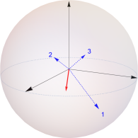
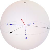
(a) Generic State

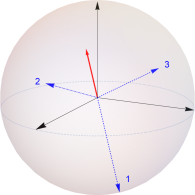
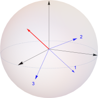
(b) Pure State

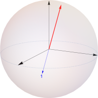
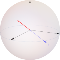
(c) Product State

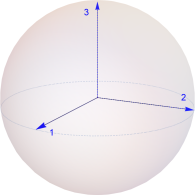
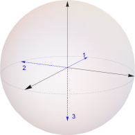
(d) Singlet State

Figure 2: The Bloch spheres of the two subsystems for: (a) generic state, (b) pure state, (c) product state, and (d) singlet state. In each Bloch sphere, the local Cartesian axes vectors are in black, the subsystem’s Bloch vector is in red, and the scaled correlation axes ($x_{i}\hat{m}_{i}$ or $x_{i}\hat{n}_{i}$) dashed in blue. The scaled correlation axes are mutually orthogonal in each Bloch sphere, and are labeled with their index $i$ to indicate the correlation pairing between the two Bloch spheres.

The ambiguities of the SVD are better understood in the diagrammatic representations above. Reordering the singular values and singular vectors corresponds to a simple relabeling of the scaled correlation axes. One may freely flip the signs of any two paired correlation axes, since measurements in the negative direction of both subsystems will still be positively correlated. If two scaled correlation axes have the same length, an identical rotation about the third axis may be applied to them in both Bloch spheres. For example, axes $2$ and $3$ in both spheres for the pure state may be rotated by the same arbitrary angle about axis $1$, leaving the underlying quantum correlations unaffected.

Although any two-qubit quantum state can be represented as a pair of correlated Bloch spheres, not every possible configuration of Bloch vectors and scaled correlation axes represents a physically allowed quantum state. For a state to be physically allowed, it must satisfy the positivity inequalities (62). Since the latter depend on the relative not absolute Bloch vectors, one may arbitrarily rotate a Bloch sphere as a single unit (along with its Bloch vector and correlation axes) without affecting the physicality of a state.

While the Bloch sphere pairs help us visualize individual quantum states, Sec. IX is dedicated to visualizing the entire quantum state space.

VI Unitary Operations

VI.1 Local unitary transformations

In this section we investigate the effect of unitary operations on the Bloch matrix components as well as the singular value decomposition. We begin with local unitary operations.

We showed in (18) that a single qubit unitary transformation is equivalent to a rotation of the Bloch vector. Let $U_{1}$ and $U_{2}$ be $2\times 2$ unitary matrices with unitary transformations corresponding to rotation matrices $Q_{1}$ and $Q_{2}$ respectively. It is straightforward to show that applying a local unitary transformation to the quantum state, $\rho\rightarrow\rho^{\prime}=(U_{1}\otimes U_{2})\rho(U_{1}^{\dagger}\otimes U_{2}^{\dagger})$, is equivalent to the following transformations on the Bloch matrix components (Horodecki and Horodecki, 1996; Makhlin, 2002):

$$\vec{u} \rightarrow\vec{u}^{\prime}=Q_{1}\vec{u},$$

$$\vec{v} \rightarrow\vec{v}^{\prime}=Q_{2}\vec{v},$$

$$R \rightarrow R^{\prime}=Q_{1}RQ_{2}^{\dagger},$$ (63)

where the primed symbols indicate the value after the transformation. The local Bloch vectors are rotated as expected, while the first rotation is applied to the rows of the correlation matrix, and the second to its columns.

Since $Q_{i}$ are rotations, they satisfy $\det Q_{i}=1$ and $Q_{i}^{\dagger}Q_{i}=I$. With this in mind, it easy to show that the transformations (63) leave every term in the positivity inequalities (54) unchanged. It is to be expected of course that local unitary transformations do not affect positivity. Nonetheless, it is interesting that even the individual terms in the inequalities are unaffected.

It becomes clear why this is the case when we examine the effect of local unitary transformations in the SVD picture. The modified correlation matrix can be expressed in its own SVD, $R^{\prime}=Q_{1}M\Sigma N^{\dagger}Q_{2}^{\dagger}\equiv M^{\prime}\Sigma N^{\prime\dagger},$ with $M^{\prime}\equiv Q_{1}M$ and $N^{\prime}\equiv Q_{2}N$ themselves orthogonal matrices. The relative Bloch vectors are left unaffected by the transformation, as per $\vec{g}^{\prime}=M^{\prime\dagger}\vec{u}^{\prime}=M^{\dagger}Q_{1}^{\dagger}Q_{1}\vec{u}=M^{\dagger}\vec{u}=\vec{g},$ with a similar result for $\vec{h}$. The orientation is likewise unaffected with $d^{\prime}=\det(Q_{1})\det(Q_{2})d=d$.

The effect of the local unitary transformation is then

$$M \rightarrow M^{\prime}=Q_{1}M,$$

$$N \rightarrow N^{\prime}=Q_{2}N,$$ (64)

with $\Sigma,\vec{g},\vec{h},d$ left unchanged. Only the unaffected degrees of freedom are present in the positivity inequalities (62), explaining why even their individual terms are left unchanged. This representation describes in a simpler manner the local unitary invariants derived in Ref. (Makhlin, 2002).

In the paired Bloch sphere diagrams, a local unitary transformation rotates the Bloch vector and correlation axes in each sphere together, leaving the relative Bloch vectors unchanged. Equivalently, the reverse rotation may be applied to the absolute axes in each sphere.

There are two senses in which we speak of “local degrees of freedom”. We may mean the degrees of freedom that are locally measurable. These are simply the Bloch vectors $\vec{u},\vec{v}$. We may also mean the degrees of freedom that are free to vary via local unitary transformations. That is, the orthogonal matrices $M,N$, with the product of their determinants, the orientation $d$, left unchanged.

VI.2 General unitary transformations

We now consider the effect of general unitary operations on the composite quantum state. Ideally, we would like to represent an arbitrary unitary operator $U\in\text{SU}(4)$, as a combination of local and nonlocal unitary transformations. A powerful result by Zhang et al. (Zhang et al., 2003) fulfills this requirement, stating that any such $U$ can be written as

$$U=\left(U_{1}\otimes U_{2}\right)\mathring{U}\big{(}\theta_{1},\theta_{2},\theta_{3}\big{)}\left(U_{3}\otimes U_{4}\right),$$ (65)

where the $U_{k}$ are single-qubit unitary operators, and $\mathring{U}\big{(}\theta_{1},\theta_{2},\theta_{3}\big{)}$, which we call a basic nonlocal operator, is given by

$$\mathring{U}=\exp\left[\frac{i}{2}\left(\theta_{1}\sigma_{1}{\otimes}\sigma_{1}+\theta_{2}\sigma_{2}{\otimes}\sigma_{2}+\theta_{3}\sigma_{3}{\otimes}\sigma_{3}\right)\right].$$ (66)

In other words, a generic unitary transformation can be reduced to a local transformation, followed by a basic nonlocal transformation, followed by another unitary transformation, with $6$, $3$, and $6$ degrees of freedom respectively. In the previous section we examined the effect of local unitary transformations, and therefore only need to consider the effect of a basic nonlocal operator $\mathring{U}$. The above representation is not necessarily unique (Zhang et al., 2003), however this is of no consequence for our purposes.

Since the three $\sigma_{j}\otimes\sigma_{j}$ commute, the matrix exponential of their sum is simply the product of their matrix exponentials, in any order. It is therefore possible to factorize $\mathring{U}$ to the product of three exponentials,

$$\mathring{U}\big{(}\theta_{1},\theta_{2},\theta_{3}\big{)}=\mathring{U}_{1}\big{(}\theta_{1}\big{)}\mathring{U}_{2}\big{(}\theta_{2}\big{)}\mathring{U}_{3}\big{(}\theta_{3}\big{)},$$ (67)

where the $\mathring{U}_{j}$, called irreducible nonlocal operators, are given by

$$\mathring{U}_{j}\big{(}\theta_{j}\big{)}=\exp\left[\frac{i}{2}\theta_{j}\sigma_{j}{\otimes}\sigma_{j}\right],\quad j=1,2,3.$$ (68)

To understand the action of nonlocal operations, we examine the effect of one of the irreducible nonlocal transformations, say $\mathring{U}_{1}$, with the understanding that $\mathring{U}_{2}$ and $\mathring{U}_{3}$ will be of similar effect. With much algebra, some of which is shown in Appendix C, the transformation $\rho\rightarrow\rho^{\prime}=\mathring{U}_{1}\rho\mathring{U}_{1}^{\dagger}$ can be shown to transform the Bloch matrix  $r$  $\mkern-2.1mu\mathchar 382\relax$ $\mkern-2.1mu\mathchar 382\relax$    in the following manner:

$$\leavevmode\hbox{\hskip 2.39468pt\leavevmode\hbox{$r$}\raisebox{0.10555pt}{$\,\smash{\leavevmode\hbox{\hskip 1.91669pt\leavevmode\hbox{$\mkern-2.1mu\mathchar 382\relax$}\raisebox{12.33888pt}{$\rotatebox{180.0}{$\mkern-2.1mu\mathchar 382\relax$}$}\hskip 1.91669pt}}$}\hskip 2.39468pt}\rightarrow\leavevmode\hbox{\hskip 2.39468pt\leavevmode\hbox{$r$}\raisebox{0.10555pt}{$\,\smash{\leavevmode\hbox{\hskip 1.91669pt\leavevmode\hbox{$\mkern-2.1mu\mathchar 382\relax$}\raisebox{12.33888pt}{$\rotatebox{180.0}{$\mkern-2.1mu\mathchar 382\relax$}$}\hskip 1.91669pt}}$}\hskip 2.39468pt}^{\prime}=\begin{bmatrix}1&v_{1}&\hphantom{-}v_{2}\cos\theta_{1}+R_{13}\sin\theta_{1}&\hphantom{-}v_{3}\cos\theta_{1}-R_{12}\sin\theta_{1}\\ u_{1}&R_{11}&\hphantom{-}v_{3}\sin\theta_{1}+R_{12}\cos\theta_{1}&-v_{2}\sin\theta_{1}+R_{13}\cos\theta_{1}\\ u_{2}\cos\theta_{1}+R_{31}\sin\theta_{1}&\hphantom{-}u_{3}\sin\theta_{1}+R_{21}\cos\theta_{1}&R_{22}&R_{23}\\ u_{3}\cos\theta_{1}-R_{21}\sin\theta_{1}&-u_{2}\sin\theta_{1}+R_{31}\cos\theta_{1}&R_{32}&R_{33}\end{bmatrix}.$$ (69)

One can interpret the operation $\mathring{U}_{1}$ as resulting in four two-variable “mixing” operations, where each mixture is the mathematical application of the two-dimensional rotation matrix $\left[\begin{smallmatrix}\cos\theta&-\sin\theta\\ \sin\theta&\cos\theta\end{smallmatrix}\right]$, with $\theta$ the mixing angle, to a vector of the two mixed variables. The operation mixes $u_{2}$ with $R_{31}$ and $v_{2}$ with $R_{13}$ with a mixing angle $-\theta_{1}$, and $u_{3}$ with $R_{21}$, $v_{3}$ with $R_{12}$ with a mixing angle $\theta_{1}$.

More generally, supposing $\{i,j,k\}$ to be a cyclic permutation of $\{1,2,3\}$, the operation $\mathring{U}_{j}$ mixes $u_{k}$ with $R_{ij}$, $v_{k}$ with $R_{ji}$ with a mixing angle $-\theta_{j}$, and $u_{i}$ with $R_{kj}$, $v_{i}$ with $R_{jk}$ with a mixing angle $\theta_{j}$.

This mixing action is precisely what generates entanglement. If we start with a product state ($R_{ij}=u_{i}v_{j}$), then the modified Bloch vector for each subsystem in (69) will depend on the other system’s Bloch vector. That is, correlation was created between the two subsystems.

One may combine the effects of the three $\mathring{U}_{j}$ to find the action of $\mathring{U}$, as per (67). The effect of the basic nonlocal transformation $\rho\rightarrow\rho^{\prime}=\mathring{U}\rho\mathring{U}^{\dagger}$ on the Bloch matrix  $r$  $\mkern-2.1mu\mathchar 382\relax$ $\mkern-2.1mu\mathchar 382\relax$    is given in Appendix C.

A question that naturally arises at this point is the effect of irreducible nonlocal transformations on the SVD picture, i.e. its effect on $\Sigma,\vec{g},\vec{h},M,N$ and $d$. Since local operations only act on $M$ and $N$, one may naively hope that an irreducible nonlocal operator only acts on $\Sigma,\vec{g},\vec{h},$ and $d$. However, this cannot be the case, since it would imply that irreducible nonlocal operators commute with local operations. Given the action of $\mathring{U}_{1}$ on $\vec{u},\vec{v},R$ shown in (69), there is no simple way to represent its effect on the SVD components.

We demonstrate this by plotting the effect of $\mathring{U}_{1}(\theta_{1})$ on the singular values of a randomly generated quantum state in Fig. 3. The singular values change with a period $\pi$. We also see that $\mathring{U}_{1}$ has an effect on the singular values akin to avoided crossings of Hermitian operator eigenvalues (von Neumann and Wigner, 1929). In the region in parameter-space where the avoided crossing between singular values $x_{i}$ and $x_{j}$ takes place, one can show that their respective primary correlation axes undergo a rapid but continuous transformation roughly with the net effect that they switch places; $\hat{m}_{i}\longleftrightarrow\hat{m}_{j},$ and $\hat{n}_{i}\longleftrightarrow\hat{n}_{j}$. For some special choices of initial state, (or with a simultaneous application of $\mathring{U}_{2}$ and/or $\mathring{U}_{3}$) one can get actual crossings.

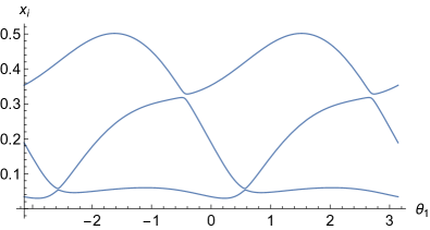
Figure 3: The effect of the irreducible nonlocal unitary transformation due to $\mathring{U}_{1}(\theta_{1})$ on a generic quantum state. The three singular values $x_{i}$ are plotted against the parameter angle $\theta_{1}$ in the domain $[-\pi,\pi]$.

The above figure simplifies somewhat for pure states, and more so for maximally entangled states. However, the action of $\mathring{U}_{1}$ on the SVD components cannot, in general, be given in a form that is simpler than its action on the Bloch matrix components in (69).

VI.3 Unitary invariants

For a $4\times 4$ matrix there are exactly four invariant quantities unchanged by unitary transformations. The invariants of a density matrix $\rho$ may be taken as its eigenvalues $\lambda_{1},\lambda_{2},\lambda_{3},\lambda_{4}$. Alternatively, since functions of invariants are themselves invariant, one may take $\operatorname{Tr}\rho,\operatorname{Tr}\rho^{2},\operatorname{Tr}\rho^{3},\operatorname{Tr}\rho^{4}$ as the trace unitary invariants. Since $\operatorname{Tr}\rho=1$, the values of the three other traces define an equivalence class of density matrices. Unitary transformations can take a density matrix to any other in its equivalence class, but not to one in another class.

One may also find three invariants in terms of the Bloch matrix components. Given their derivation from $\operatorname{Tr}\rho^{n}$, it is clear that the left hand sides of the positivity inequalities (54) or (62), are unitarily invariant. We call these the positivity unitary invariants, as their values indicate how far the state is from violating positivity.

We can further simplify these by extracting from them three independent invariants, similar to those in (Englert and Metwally, 2001), which we call the Bloch invariants, given by

$$B_{1} \equiv\|\leavevmode\hbox{\hskip 2.39468pt\leavevmode\hbox{$r$}\raisebox{0.10555pt}{$\,\smash{\leavevmode\hbox{\hskip 1.91669pt\leavevmode\hbox{$\mkern-2.1mu\mathchar 382\relax$}\raisebox{12.33888pt}{$\rotatebox{180.0}{$\mkern-2.1mu\mathchar 382\relax$}$}\hskip 1.91669pt}}$}\hskip 2.39468pt}\|^{2},$$

$$B_{2} \equiv\vec{u}{}^{\dagger}R\vec{v}-\det R=\vec{g}{}^{\dagger}\Sigma\vec{h}-d\det\Sigma,$$

$$B_{3} \equiv\|\vec{u}\|^{2}\|\vec{v}\|^{2}+\|\vec{u}{}^{\dagger}R\|^{2}+\|R\vec{v}\|^{2}+\|\tilde{R}\|^{2}-2\vec{u}{}^{\dagger}\tilde{R}\vec{v}$$

$$=\|\vec{g}\|^{2}\|\vec{h}\|^{2}+\|\Sigma\vec{g}\|^{2}+\|\Sigma\vec{h}\|^{2}+\|\tilde{\Sigma}\|^{2}-2d\vec{g}{}^{\dagger}\tilde{\Sigma}\vec{h}.$$ (70)

Thus, there are different levels of invariance. Local unitary transformations will leave nine continuous degrees of freedom $\Sigma,\vec{g},\vec{h}$ as well as the discrete $d$ invariant (Makhlin, 2002; Grassl et al., 1998). A general (nonlocal) unitary transformation will leave the three degrees of freedom in the Bloch invariants $B_{1},B_{2},B_{3}$ unchanged. The noteworthy feature of the expressions in (70) is that they express the general unitary invariants in terms of the local unitary invariants.

If the quantum state undergoes non-unitary evolution, as in open system dynamics (Breuer and Petruccione, 2007) or depolarizing noise channels, then even the Bloch invariants $B_{i}$ will change.

Interestingly, $B_{i}$ is of order $i+1$ in the Bloch matrix terms. If the quantum state is acted upon by a depolarizing noise channel $\rho\rightarrow\rho^{\prime}=p\rho+(1-p)\frac{I}{4}$, with $(1-p)$ the noise ratio, then the Bloch invariants change as $B_{i}\rightarrow p^{i+1}B_{i}$.

VII Entanglement Criteria

A quantum state $\rho$ is defined as separable if it can be written as a convex combination of product states,

$$\rho=\sum_{i}p_{i}\rho_{i}^{(1)}\otimes\rho_{i}^{(2)},$$ (71)

where $p_{i}$ are non-negative probabilities that sum to unity. A state that is not separable is defined as entangled.

Given a quantum state, it is important to find out whether or not it is entangled. To this end, one can use the positive partial transpose (PPT) criterion, also known as the Peres-Horodecki criterion. It was first stated by Woronowicz (Woronowicz, 1976) based on previous work by Stï¿œrmer (Størmer, 1963), and extended for use in quantum systems by Peres and Horodecki (Peres, 1996; Horodecki et al., 1996). The PPT criterion states that if one takes the transpose of one subsystem (i.e. partial transpose) of the density matrix $\rho$, and the resulting matrix is not positive (i.e. has a negative eigenvalue), then $\rho$ was entangled. This criterion is necessary and sufficient for entanglement in the two-qubit systems addressed in this paper, and sufficient for higher dimensions.

We apply the PPT criterion in the Bloch matrix picture. First we note that taking the transpose of the extended Pauli matrices leaves $\sigma_{0},\sigma_{1},\sigma_{3}$ unchanged, and flips the sign of $\sigma_{2}$. Therefore, transposing a single-qubit density matrix is equivalent to flipping the sign of the second entry of the Bloch vector in (13). That is, the Bloch vector transforms as $\vec{r}\rightarrow Q_{t}\vec{r}$, where

$$Q_{t}=\left[\begin{array}[]{rrr}1&0&0\\ 0&-1&0\\ 0&0&\hphantom{-}1\end{array}\right].$$ (72)

Based on this, the partial transpose of the quantum state $\rho$ with Bloch matrix components $\vec{u},\vec{v},R$ is equivalent to the transformations

$$\vec{u} \rightarrow Q_{t}\vec{u},\text{ and }R\rightarrow Q_{t}R,\text{ or}$$

$$\vec{v} \rightarrow Q_{t}\vec{v},\text{ and }R\rightarrow RQ_{t}^{\dagger},$$ (73)

where the transformations in the first (second) line signify a transpose of the first (second) subsystem. In terms of their effects on the positivity inequalities (54), the preceding transformations only reverse the signs of the $\det R$ and $\vec{u}{}^{\dagger}\tilde{R}\vec{v}$ terms.

To interpret this result, it is more instructive to examine the partial transpose operation in the SVD picture. Following the example of local unitary transformations in (64), it is easy to show that the partial transpose transformations in (73) are equivalent to

$$M \rightarrow Q_{t}M,\text{ or}$$

$$N \rightarrow Q_{t}N,$$ (74)

with $\Sigma,\vec{g},\vec{h},$ left unchanged. The effect of either of the above is to flip the orientation $d\rightarrow\det Q_{t}d=-d$.

The next step is to examine whether the partially transposed state violates positivity. Given the above, the only change to the positivity inequalities (62) by the partial transpose operation is to flip the sign of $d$. If after the orientation $d$ is reversed, all the positivity inequalities remain satisfied, then the initial state was separable, otherwise it was entangled.

Therefore, the only meaningful effect of the partial transpose is to flip the sign of the orientation $d$. This may be alternatively achieved if $Q_{t}$ is replaced by any orthogonal matrix $Q_{-}$ such that $\det Q_{-}=-1$. Given some quantum state, we call the quantum state with identical $\Sigma,\vec{g},\vec{h},$ but the reverse orientation $d$ its conjugate state. Testing the entanglement of a quantum state is equivalent to testing the positivity of its conjugate state.

The partial transpose may be replaced by other testing operations with the same effect. For example, a partial anti-diagonal transpose, corresponding to $Q_{-}=\operatorname{diag}(1,1,-1)$, would work just as well. Every choice of $Q_{-}$ corresponds to a new criterion. Though the standard PPT criterion and its anti-diagonal version are the simplest to apply to $\rho$, others may possibly be more convenient under some assumptions.

If we think of our qubits as spin-$\frac{1}{2}$ systems, the axes in the Bloch sphere correspond to three spatial dimensions. In this case, the entanglement criterion corresponds to applying the rotoreflection $Q_{-}$ to one subsystem’s spin and testing the physicality of the result, similar to the mirror quantum theory of Ref. (Hoehn, 2014). Separable states may be interpreted as ones whose spin mirror image in one subsystem are physical, while for entangled states the single subsystem spin mirror images are unphysical. This makes sense when one recalls the spin of a member of an entangled pair is not simply an isolated vector in space, but rather a spatial distribution of correlations.

Reflecting the spin can be thought of as a combination of spatial parity (P) inversion and time (T) inversion, common in quantum field theory (Peskin and Schroeder, 1995). However, it is important to note that this PT inversion is applied to a single subsystem of the two, not the combined state as is usually the case. Reflections become more difficult to intuit if our qubits are not spin-$\frac{1}{2}$ systems, but for example, two-level atoms where the Bloch vectors don’t correspond to spatial directions. In this case, reflections are simply taken abstractly over the Bloch vector space.

Applying an entangling unitary operation will leave the invariants in (70) unchanged, but the individual terms in the positivity equation will change such that entanglement criteria are satisfied. For example, an entangling unitary transformation will change the two quantities $\vec{u}{}^{\dagger}R\vec{v}=\vec{g}{}^{\dagger}\Sigma\vec{h}$ and $\det R=d\det\Sigma$ by the same amount such that their difference, the invariant $B_{2}$, remains unchanged. However, the change may be such that reversing the sign of the second expression will lead to a violation of the positivity inequalities, and hence the transformed state is entangled.

Quantum states where $R$ (or $\Sigma$) is of rank $1$ or $0$ cannot be entangled, since the two terms whose sign is flipped will be zero, and the satisfied positivity inequalities remain unchanged. Even rank $2$ states where $\vec{u}{}^{\dagger}\tilde{R}\vec{v}=d\vec{g}{}^{\dagger}\tilde{\Sigma}\vec{h}=0$ cannot be entangled.

For a maximally entangled Bell state, the values of the left hand sides of the positivity inequalities (62), after the reversal of the orientation, are $0,-4,-16$ respectively. These are “the most negative” values these quantities can attain for any quantum state. The first has no $d$ dependence and of course is never negative for any state. It is also quite common for only the third quantity to be negative for an entangled state (e.g. $\vec{u}=\vec{v}=0,\,R=-0.4I$). Although it remains to be rigorously verified, there do not seem to be physical quantum states where the second is negative but the third is not. One may therefore consider the degree of negativity of the left hand side of the third inequality (62c), after orientation reversal $d\rightarrow-d$, as a possible candidate for degree of entanglement.

There remains the important question of whether unphysicality under reflection is fundamental to entanglement, or just an artifact of the two-qubit system. In bipartite systems larger than a qubit-qutrit pair, the PPT criterion is sufficient but not necessary. For such systems, a subsystem’s Bloch vector space may have eight or more dimensions. Perhaps more feasibly, one can also speculate about multipartite entanglement between $n$ qubits. The Bloch matrix will then become a tensor with $4^{n}$ entries. Unfortunately, useful analysis will be complicated by the lack of a simple singular value decomposition in higher dimensions (Tucker, 1966; Kolda and Bader, 2009). Despite this, one may hypothesize multiple generalized orientation parameters $d$ in higher dimensions. If they exist, perhaps inverting them will provide workable entanglement criteria.

VIII Special Classes of States

VIII.1 Maximally Entangled states

In this section we find the Bloch matrix description for some important classes of states. We begin by characterizing maximally entangled states, a class that includes Bell states. A maximally entangled state may be defined as being (i) pure, and (ii) locally maximally mixed (LMM), i.e. once a partial trace eliminates one subsystem, the other is left in a maximally mixed state.

A pure density matrix $\rho$ has a single nonzero eigenvalue, equal to unity. From the derivation of the in Sec. IV, it is clear that achieving purity is equivalent to all three positivity inequalities achieving equality. The LMM condition is equivalent to both local Bloch vectors being zero. Setting $\vec{g}=\vec{h}=0$ and equality in (62), we have

$$\|\Sigma\|^{2}=x_{1}^{2}+x_{2}^{2}+x_{3}^{2}=3,$$

$$d\det\Sigma=dx_{1}x_{2}x_{3}=-1,$$

$$\|\tilde{\Sigma}\|^{2}=x_{2}^{2}x_{3}^{2}+x_{3}^{2}x_{1}^{2}+x_{1}^{2}x_{2}^{2}=3.$$ (75)

Given that $x_{i}\geq 0$, the only solution to the above is $d=-1$ and $x_{1}=x_{2}=x_{3}=1$. That is, $\Sigma=I$. Therefore

$$R=MN^{\dagger}\equiv O_{-},$$ (76)

where $O_{-}$ is an orthogonal matrix with $\det O_{-}=d=-1$.

Maximally entangled states are characterized as those whose local Bloch vectors $\vec{u},\vec{v}$ are zero, and whose correlation matrix $R$ is orthogonal with determinant $-1$, conditions clearly satisfied by the Bell states (32).

The uniqueness of $\Sigma,\vec{g},\vec{h},$ and $d$ in the above solution implies that there exists a single maximally entangled state, unique up to local unitary transformations.

VIII.2 Pure states

As mentioned above, requiring that the positivity inequalities (62) achieve equality suffices to characterize pure states. However, solving the resulting equalities is in general algebraically involved. It is easier to note that any pure state can be reached from another by the action of an arbitrary unitary transformation, as the latter do not affect purity.

There are $7$ degrees of freedom in bipartite pure states: $2$ for each of the $4$ complex coefficients, less one for an irrelevant global phase. Local unitary operations create $6$ of the $7$, and so we expect basic nonlocal unitary operation $\mathring{U}$ to effect the remaining degree of freedom. Since $\Sigma,\vec{g},\vec{h},d$ are invariant under local unitaries, we can start with their values for a known pure state and then apply $\mathring{U}$, expecting it to generate the final degree of freedom on these quantities.

Therefore we start with the pure state $\vec{g}=\vec{h}=\vec{u}=\vec{v}=(1,0,0),$ and $\Sigma=R=\operatorname{diag}(1,0,0)$. Applying $\mathring{U}\big{(}\theta_{1},\theta_{2},\theta_{3}\big{)}$, whose effect on the Bloch components is shown in (97), to this state:

$$\vec{u}^{\prime}=\vec{v}^{\prime} =(\cos\theta,0,0),$$

$$R^{\prime} =\begin{bmatrix}1&0&0\\ 0&0&\sin\theta\\ 0&\sin\theta&0\end{bmatrix},$$

where $\theta=\theta_{2}-\theta_{3}$. As expected, the resulting pure state has a single degree of freedom defined by $\theta$. The above correlation matrix has the singular value decomposition $R^{\prime}=M^{\prime}\Sigma^{\prime}N^{\prime\dagger}$ where $M^{\prime}=\left[\begin{smallmatrix}1&0&0\\ 0&0&1\\ 0&1&0\end{smallmatrix}\right]$, $N^{\prime}=I$ and $\Sigma^{\prime}=\operatorname{diag}(1,\sin\theta,\sin\theta)$. We also find $d=\det(M^{\prime})\det(N^{\prime})=-1$, $\vec{g}^{\prime}=M^{\prime\dagger}\vec{u}^{\prime}=\vec{u}^{\prime}$, and $\vec{h}^{\prime}=N^{\prime\dagger}\vec{v}^{\prime}=\vec{v}^{\prime}$.

Therefore pure states are characterized by

$$\vec{g} =\vec{h}=(\cos\theta,0,0),$$

$$\Sigma =\operatorname{diag}(1,\sin\theta,\sin\theta),$$

$$d =-1,$$ (77)

for some arbitrary $\theta$, up to an identical reordering of the entries in $\Sigma,\vec{g},\vec{h}$. The single nonlocal degree of freedom in (77) along with $6$ local ones in the choice of $M,N$ (so long as they satisfy $d=-1$) make up the $7$ degrees of freedom in pure states.

One can substitute (77) into the positivity inequalities (62) and verify they all satisfy equality. The pure state defined in (77) is a product state if $\theta=0$ (the state we started with) and maximally entangled when $\theta=\frac{\pi}{2}$. Hence, the quantity $\sin\theta$ may be taken as measure of entanglement for pure states.

VIII.3 Generalized isotropic states

Werner states are defined as invariant under local unitary transformations of the form $U\otimes U$ (Werner, 1989). In two-qubit systems, their density matrix takes the well known form

$$\rho_{wer}(z)=\frac{1-z}{4}I+z|\Psi^{-}\rangle\langle\Psi^{-}|,$$ (78)

where $z$ is a scalar parameter. Similarly, isotropic state are defined as invariant under local unitary transformations of the form $U\otimes U^{*}$, with density matrix of the form

$$\rho_{iso}(z)=\frac{1-z}{4}I+z|\Phi^{+}\rangle\langle\Phi^{+}|.$$ (79)

It is known that both Werner and isotropic states are physical for $-\frac{1}{3}\leq z\leq 1$ and entangled for $\frac{1}{3}\leq z$. More inclusively, we define generalized isotropic states as those invariant under local unitary transformations of the form $U_{\hat{a},\alpha}\otimes U_{\hat{b},\beta}$, where the unitary transforms are defined in (16), $\hat{a},\alpha$ vary freely, and $\hat{b},\beta$ are assumed to be one-to-one functions of $\hat{a},\alpha$. The Bloch matrix components $\vec{u},\vec{v},R$, of the invariant state should satisfy

$$\vec{u}^{\prime} =Q(\hat{a},\alpha)\vec{u}=\vec{u},$$

$$\vec{v}^{\prime} =Q(\hat{b},\beta)\vec{v}=\vec{v},$$

$$R^{\prime} =Q(\hat{a},\alpha)RQ^{\dagger}(\hat{b},\beta)=R,$$ (80)

and $Q$ are rotations with the specified parameters.

The above should hold for all $\hat{a},\alpha$, and all $\hat{b},\beta$, with some relationship to be found between the two pairs. Therefore $\vec{u}=\vec{v}=0$, as the zero vector is the only one invariant under all rotations. Further, $R$ then satisfies

$$Q(\hat{a},\alpha)RR^{\dagger}Q^{\dagger}(\hat{a},\alpha) =RR^{\dagger},$$

$$Q(\hat{b},\beta)R^{\dagger}RQ^{\dagger}(\hat{b},\beta) =R^{\dagger}R.$$

The two equalities above mean that $RR^{\dagger}$ and $R^{\dagger}R$ are invariant under any orthogonal change of basis. The only such matrices are proportional to the identity. Given that $RR^{\dagger}$ and $R^{\dagger}R$ are positive with the same magnitude, they both have the same positive proportionality constant. Hence we can write

$$RR^{\dagger}=R^{\dagger}R=z^{2}I,$$ (81)

where $z$ is some real scalar. This implies that $R=zO$ for some orthogonal $O$. Substituting this in the last equality in (80) and rearranging, we have

$$Q(\hat{a},\alpha)=OQ(\hat{b},\beta)O^{\dagger}.$$

Making use of the explicit expression for a rotation in (18), the last equation reduces to

$$\cos\alpha I+(1-\cos\alpha)\hat{a}\hat{a}^{\dagger}+\sin\alpha\lfloor\hat{a}\rfloor_{\times}\\ =\cos\beta I+(1-\cos\beta)O\hat{b}(O\hat{b})^{\dagger}+\sin\alpha O\lfloor\hat{b}\rfloor_{\times}O^{\dagger}.$$ (82)

Taking the trace of both sides, $\cos\alpha=\cos\beta\Rightarrow\alpha=\pm\beta.$ Without loss of generality, set $\alpha=\beta$. Then (82) implies

$$\hat{a}\hat{a}^{\dagger} =O\hat{b}(O\hat{b})^{\dagger},$$ (83)

$$\lfloor\hat{a}\rfloor_{\times} =O\lfloor\hat{b}\rfloor_{\times}O^{\dagger}.$$ (84)

Multiplying (83) by $\hat{a}$ from both sides yields $(\hat{a}^{\dagger}O\hat{b})^{2}=1.$ Noting that the indices of the cross product matrix satisfy $\big{(}\lfloor\hat{a}\rfloor_{\times}\big{)}_{ij}=\varepsilon_{jik}a_{k}$, (84) then implies

$$\varepsilon_{jik}a_{k} =O_{im}\varepsilon_{nml}b_{l}O_{jn}$$

$$=\varepsilon_{jik}\det(O)O_{kl}b_{l},$$ (85)

where we have used (94) with $O^{\dagger}$ in the place of $O$. Canceling the Levi-Civita factor, (85) is equivalent to $\hat{a}=(\det O)O\hat{b}$. More symmetrically,

$$\hat{a}^{\dagger}O\hat{b}=\det O.$$ (86)

Therefore, a generalized isotropic state is defined as invariant under $U_{\hat{a},\alpha}\otimes U_{\hat{b},\alpha}$ for any angle $\alpha,$ and any $\hat{a},\hat{b}$ satisfying (86) for some fixed orthogonal $O$. Explicitly, the state has Bloch matrix components

$$\vec{u}=\vec{v}=0,\,R=zO.$$ (87)

Without loss of generality, choose $\det O=-1$, the sign of $z$ offsetting our choice. Finally, we find the range of $z$ for which the general isotropic state is positive or entangled. Note that (44) implies the cofactor matrix is $\tilde{R}=-z^{2}O$. Substituting (87) into the positivity equations (54),

$$1-z^{2}\geq 0,$$

$$2z^{3}-3z^{2}+1\geq 0,$$

$$-3z^{4}+8z^{3}-6z^{2}+1\geq 0.$$ (88)

The polynomials on the left hand side appear in Ref. (Byrd and Khaneja, 2003), though apply more generally here. The first inequality simplifies to $-1\leq z\leq 1$ . The last two factor to

$$(1-z)^{2}(2z+1)\geq 0,$$

$$(1-z)^{3}(3z+1)\geq 0.$$ (89)

The last inequality is satisfied for

$$-\frac{1}{3}\leq z\leq 1,$$ (90)

which is the range for $z$ common to all three inequalities.

To check for entanglement, we apply the positivity criterion from Sec. VII, which amounts to flipping the sign of $z$ in the inequalities (88). Reproducing the steps above with sign reversal, we conclude that the state is separable for $-1\leq z\leq\frac{1}{3}$ and entangled for

$$\frac{1}{3}<z.$$ (91)

Section VIII.1 showed that an orthogonal matrix with negative determinant characterizes the correlation matrix of all maximally entangled states. Therefore, a general isotropic state takes the form

$$\rho_{GI}(z)=\frac{1-z}{4}I+z|\Psi\rangle\langle\Psi|,$$ (92)

where $|\Psi\rangle$ is any maximally entangled state. Given (90) and (91), $\rho_{GI}(z)$ is positive for $-\frac{1}{3}\leq z\leq 1$, and entangled for $\frac{1}{3}<z$. This successfully generalizes Werner and isotropic states, reproducing their parameter ranges.

IX Geometry of The State Space

It is instructive to use the results thus far to visualize the quantum state space. We draw the regions of physically allowable quantum states, where the positivity inequalities (62) hold. As the latter are functions only of $\Sigma,\vec{g},\vec{h},$ $d$, each point in our diagrams will represent a family of states equivalent up to local unitary operations.

There are $9$ continuous degrees of freedom in the aforementioned variables, we hold constant $6$ and plot the physical regions for the remaining $3$. We create two types of diagrams, singular value diagrams, with $\vec{g}$ and $\vec{h}$ constant the singular values $x_{1},x_{2},x_{3}$ along the diagonal of $\Sigma$ varying on the axes, and relative Bloch vector diagrams, with $\Sigma$ and $\vec{h}$ constant the components of $\vec{g}$ varying on the axes.

In each case, regions are plotted twice; once for each value of the orientation $d$. Regions with $d=1$ are colored in blue and $d=-1$ in red. As per the entanglement criterion in Sec. VII, states in the the intersection of the two regions are separable, and states in one region but not the other are entangled.

It can be shown that all three positivity inequalities are needed, in the sense that no two among them imply the third, in general. However, it is the third inequality that determines the surface of the convex allowable region; while the other two eliminate superfluous disconnected regions. Since the third positivity inequality contains terms up to the fourth power, the allowable regions are bordered by a family of quartic surfaces (Jessop, 1916).

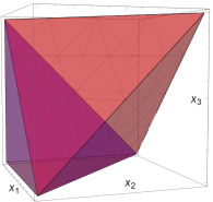
(a) $\vec{g}=\vec{h}=(0,0,0)$

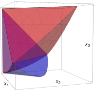
(b) $\vec{g}=\vec{h}=(0,0,0.5)$

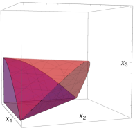
(c) $\vec{g}=(0,0,0.5)$   $\>\vec{h}=(0,0,0)$

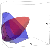
(d) $\vec{g}=\vec{h}=(0.3,0.3,0.3)$

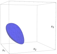
(e) $\vec{g}=(0.4,0.4,0.4)$  $\>\vec{h}=(0.3,0.3,0.3)$

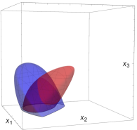
(f) $\vec{g}=(-0.4,-0.5,0.2)$  $\vec{h}=(-0.33,-0.33,0.1)$

Figure 4: Singular value diagrams: The regions in singular value space $x_{1},x_{2},x_{3}$ where positivity is satisfied, for fixed values of $\vec{g}$ and $\vec{h}$. Bounded by the unit cube, with the origin in the rear bottom left. Regions with $d=1$ in blue and $d=-1$ in red.

Figure 4 contains the singular value diagrams for several values of $\vec{g}$ and $\vec{h}$. The most interesting is Fig. 4a, where both local Bloch vectors are zero, i.e. LMM states. In this case, the last positivity inequality (62c) factors to

$$(d{-}x_{1}{+}x_{2}{+}x_{3})(d{+}x_{1}{-}x_{2}{+}x_{3})\times\qquad$$

$$\qquad(d{+}x_{1}{+}x_{2}{-}x_{3})(d{-}x_{1}{-}x_{2}{-}x_{3})\geq 0,$$ (93)

which describes a tetrahedral region bounded by four planes for $d=\pm 1$. If $x_{i}$ were allowed to go negative, the vertices would be $(-d,d,d)$, $(d,-d,d)$, $(d,d,-d)$, and $(-d,-d,-d)$. This “large” tetrahedron is analogous to the one usually representing linear combinations of Bell states, with a Bell state at each vertex (Horodecki and Horodecki, 1996; Bertlmann et al., 2002; Spengler et al., 2011). One can see this if $d=1$, whence the vertex coordinates are the diagonals of Bell state correlation matrices in (32).

However, since $x_{i}\geq 0$, only the octant in Fig. 4a is physical. The wedge bounded by points $(1,0,0)$, $(0,1,0)$, $(0,0,1)$, and $(0,0,0)$ gives the set of separable states (for both values of $d$). The “small” tetrahedron in the figure bounded by points $(1,0,0)$, $(0,1,0)$, $(0,0,1)$, and $(1,1,1)$ contains entangled states (with $d=-1$). The origin corresponds to the maximally mixed state and the point $(1,1,1)$ is the maximally entangled state, unique up to local operations. This graphical representation is more powerful than the usual one as all maximally entangled states are included in a single point.

The straight line from the origin to $(1,1,1)$ represents the generalized isotropic states of Sec. VIII.3. As expected, $\frac{1}{3}$ of this line lies in the separable region, and the rest in the entangled. The volume occupied by entangled states is double that of separable states, so by a natural measure, there are twice as many entangled as there are separable LMM states.

As the relative Bloch vectors $\vec{g}$ and $\vec{h}$ change, they continuously deform the blue and red regions as shown in the figures. Either the blue or red regions may vanish entirely, as is the case with Fig. 4e, in which case the states are all entangled.

Given the result in Sec. VIII.2, pure states must lie along the diagonal of the outer surfaces of the unit cube, and there is only a single pure state for a suitable choice of $\vec{g}=\vec{h}$. For LMM states, the pure state is the maximally entangled state. In Fig. 4b, the pure state is at the vertex of the red deformed tetrahedron at $(\frac{\sqrt{3}}{2},\frac{\sqrt{3}}{2},1)$. Product states must lie on one of the Cartesian axes.

For degenerate choices of $\vec{g}$ and $\vec{h}$, i.e., $g_{i}=g_{j}$ and $h_{i}=h_{j}$, $i\neq j$, local operations may switch the ordering of $x_{i}$ and $x_{j}$. There is threefold degeneracy in Figs. 4a, 4d and 4e, and twofold degeneracy in Figs. 4b and 4c. One may eliminate the degeneracy by restricting the singular values to a subset of the space, e.g. the region $x_{1}\geq x_{2}\geq x_{3}$ for threefold degeneracy.

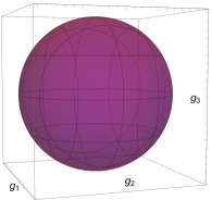
(a) $\Sigma=\operatorname{diag}(0,0,0)$  $\vec{h}=(0,0,0)$

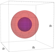
(b) $\Sigma=\operatorname{diag}(0.3,0.3,0.3)$  $\vec{h}=(0,0,0)$

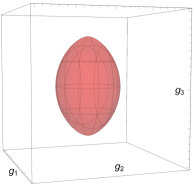
(c) $\Sigma=\operatorname{diag}(0.5,0.5,0.3)$  $\vec{h}=(0,0,0)$

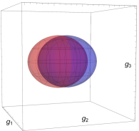
(d) $\Sigma=\operatorname{diag}(0.3,0,0.3)$  $\vec{h}=(0,0.3,0)$

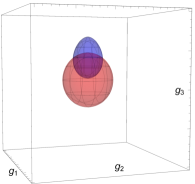
(e) $\Sigma=\operatorname{diag}(0.4,0.3,0.2)$  $\vec{h}=(0,0,0.5)$

(f) $\Sigma=\operatorname{diag}(0.25,0.3,0.3)$  $\vec{h}=(0.4,0.5,0.5)$

Figure 5: Relative Bloch vector diagrams. The coordinates of $\vec{g}=(g_{1},g_{2},g_{3})$ where positivity is satisfied, for fixed values of $\Sigma$ and $\vec{h}$. Axes in the range $[-1,1]$, with the origin at the center of the cube. Regions with $d=1$ in blue and $d=-1$ in red.

Figure 5 contains the relative Bloch vector diagrams, with allowed regions of the vector $\vec{g}$ for several fixed values of $\Sigma,\vec{h}$. Figure 5a shows the simplest case when the singular values and the second subsystem’s Bloch vector are zero. The allowed $\vec{g}$ region is a complete Bloch sphere for both values of $d$, with all the states separable. The quartic (62c) reduces to a sphere via $(\|\vec{g}\|^{2}-1)^{2}=0$.

Figure 5b shows concentric spheres, with the smaller sphere containing separable states and spherical shell between the two containing entangled states. Figure 5c shows a “football” for $d=-1$ that is entirely entangled. Figures 5d and 5e demonstrate a partial overlap between the regions for the two values of $d$. In Fig. 5f they are disjoint, meaning all the states are entangled.

X Summary

With the goal of generalizing the Bloch sphere, we have examined two-qubit systems in much detail. Representing the density matrix $\rho$ in the Dirac basis yields the Bloch matrix  $r$  $\mkern-2.1mu\mathchar 382\relax$ $\mkern-2.1mu\mathchar 382\relax$    with real entries. The latter was split to three components, the local Bloch vectors $\vec{u},\vec{v}$ and correlation matrix $R$. We then derived the positivity condition of the quantum state on $\vec{u},\vec{v},R$, in the form of three important inequalities in (54), allowing us to parametrize and visualize the quantum state space.

The form of the positivity inequalities suggested the singular value decomposition of $R$, and redefining the degrees of freedom in terms of singular value matrix $\Sigma$, singular vector matrices $M,N$ and relative Bloch vectors $\vec{g},\vec{h}$. It was found that positivity only depends on $9$ continuous degrees of freedom in $\Sigma,\vec{g},\vec{h}$ and the discrete orientation $d\equiv\det(M)\det(N)=\pm 1$, all invariant under local unitary transformations. The SVD also allowed us to visualize a quantum state as two Bloch spheres with local Bloch vectors and scaled correlation axes.

We showed that nonlocal unitary transformations have a mixing effect on the Bloch matrix components $\vec{u},\vec{v},R$. The SVD components are affected in complicated nonlocal unitaries, and the singular values can experience what resembles avoided crossings.

The three unitary invariants of the quantum state were found in terms of $\vec{u},\vec{v},R$, and in terms of $\Sigma,\vec{g},\vec{h},d$. The latter representation in particular is significant in that it represents the general unitary invariants of a state in terms of its local unitary invariants. The positive partial transpose criterion was generalized, and entanglement of a state was found equivalent to the positivity of its conjugate state, defined as the state with $\Sigma,\vec{g},\vec{h}$ unchanged and $d$ reversed in sign. We also characterized maximally entangled, pure, and generalized isotropic states.

Finally, the positivity conditions were used to visualize the quantum state space, by holding $6$ degrees of freedom in $\Sigma,\vec{g},\vec{h}$ constant, and drawing the physicality region for the other $3$. The regions were drawn for both values of orientation $d$, with the intersection indicating separable states, and the symmetric difference entangled states.

This investigation deepens our understanding of two-qubit states and aids intuition when dealing with them. Looking ahead, there are several potential extensions to this work. We may examine the effect of dissipative and open system evolution on the Bloch components, the SVD, and the unitary invariants.

One may consider the case of more qubits. Though there is no simple singular value decomposition in higher dimensions, it may prove fruitful in understanding entanglement. For instance, shedding light on the different orders of multipartite entanglement. If there turn out to be several orientation signs similar to $d$, this approach may yield an entanglement criterion that is both necessary and sufficient in higher dimensions.

Appendix A Hermitian matrix basis sets

A.1 Gell-Mann matrices (3$\times$3)

The Gell-Mann matrices, $G_{m}$, are the most widely used set of generators for the group of special unitary 3$\times$3 matrices, $SU(3)$ (Gell-Mann and Ne’eman, 1964). With the identity matrix ($G_{0}$), they form a basis for the space of 3$\times$3 Hermitian matrices:

$$\begin{aligned} G_{1}=\left(\begin{array}[]{ccc}0&1&0\\ 1&0&0\\ 0&0&0\end{array}\right),&&G_{2}=\left(\begin{array}[]{ccc}0&-i&0\\ i&0&0\\ 0&0&0\end{array}\right),\\ G_{3}=\left(\begin{array}[]{ccc}1&0&0\\ 0&-1&0\\ 0&0&0\end{array}\right),&&G_{4}=\left(\begin{array}[]{ccc}0&0&1\\ 0&0&0\\ 1&0&0\end{array}\right),\\ G_{5}=\left(\begin{array}[]{ccc}0&0&-i\\ 0&0&0\\ i&0&0\end{array}\right),&&G_{6}=\left(\begin{array}[]{ccc}0&0&0\\ 0&0&1\\ 0&1&0\end{array}\right),\\ G_{7}=\left(\begin{array}[]{ccc}0&0&0\\ 0&0&-i\\ 0&i&0\end{array}\right),&&G_{8}=\frac{1}{\sqrt{3}}\left(\begin{array}[]{ccc}1&0&0\\ 0&1&0\\ 0&0&-2\end{array}\right).\end{aligned}$$

A.2 Dirac matrices (4$\times$4)

The Dirac matrices are defined by $D_{\mu\nu}=\sigma_{\mu}\otimes\sigma_{\nu}$, $\mu,\nu=0,1,2,3$, and form a 16-element basis for the space of 4$\times$4 Hermitian matrices. Excluding the identity $D_{00}$, the remaining 15 matrices constitute a set of generators for the group of special unitary 4$\times$4 matrices, $SU(4)$. The matrices are explicitly given in Table 1.

	$0$	$1$	$2$	$3$
$0$	$\left(\begin{array}[]{cccc}1&0&0&0\\ 0&1&0&0\\ 0&0&1&0\\ 0&0&0&1\end{array}\right)$	$\left(\begin{array}[]{cccc}0&1&0&0\\ 1&0&0&0\\ 0&0&0&1\\ 0&0&1&0\end{array}\right)$	$\left(\begin{array}[]{cccc}0&-i&0&0\\ i&0&0&0\\ 0&0&0&-i\\ 0&0&i&0\end{array}\right)$	$\left(\begin{array}[]{cccc}1&0&0&0\\ 0&-1&0&0\\ 0&0&1&0\\ 0&0&0&-1\end{array}\right)$
$1$	$\left(\begin{array}[]{cccc}0&0&1&0\\ 0&0&0&1\\ 1&0&0&0\\ 0&1&0&0\end{array}\right)$	$\left(\begin{array}[]{cccc}0&0&0&1\\ 0&0&1&0\\ 0&1&0&0\\ 1&0&0&0\end{array}\right)$	$\left(\begin{array}[]{cccc}0&0&0&-i\\ 0&0&i&0\\ 0&-i&0&0\\ i&0&0&0\end{array}\right)$	$\left(\begin{array}[]{cccc}0&0&1&0\\ 0&0&0&-1\\ 1&0&0&0\\ 0&-1&0&0\end{array}\right)$
$2$	$\left(\begin{array}[]{cccc}0&0&-i&0\\ 0&0&0&-i\\ i&0&0&0\\ 0&i&0&0\end{array}\right)$	$\left(\begin{array}[]{cccc}0&0&0&-i\\ 0&0&-i&0\\ 0&i&0&0\\ i&0&0&0\end{array}\right)$	$\left(\begin{array}[]{cccc}0&0&0&-1\\ 0&0&1&0\\ 0&1&0&0\\ -1&0&0&0\end{array}\right)$	$\left(\begin{array}[]{cccc}0&0&-i&0\\ 0&0&0&i\\ i&0&0&0\\ 0&-i&0&0\end{array}\right)$
$3$	$\left(\begin{array}[]{cccc}1&0&0&0\\ 0&1&0&0\\ 0&0&-1&0\\ 0&0&0&-1\end{array}\right)$	$\left(\begin{array}[]{cccc}0&1&0&0\\ 1&0&0&0\\ 0&0&0&-1\\ 0&0&-1&0\end{array}\right)$	$\left(\begin{array}[]{cccc}0&-i&0&0\\ i&0&0&0\\ 0&0&0&i\\ 0&0&-i&0\end{array}\right)$	$\left(\begin{array}[]{cccc}1&0&0&0\\ 0&-1&0&0\\ 0&0&-1&0\\ 0&0&0&1\end{array}\right)$

Table 1: The Dirac Matrices, $D_{\mu\nu}=\sigma_{\mu}\otimes\sigma_{\nu}$.

Aside, the gamma matrices, standard in modern treatments of the Dirac equation (Peskin and Schroeder, 1995), are given by $\gamma^{0}=D_{30},\,\gamma^{1}=iD_{21},\,\gamma^{2}=iD_{22},\,\gamma^{3}=iD_{23},\,\gamma^{5}=D_{10}$.

Appendix B Cofactor matrix singular value decomposition

We show that for any $R=M\Sigma N^{\dagger},$ its cofactor matrix satisfies $\tilde{R}=\det(M)\det(N)M\tilde{\Sigma}N^{\dagger}$, where $\tilde{\Sigma}=\operatorname{diag}(x_{2}x_{3},x_{3}x_{1},x_{1}x_{2})$ is the cofactor matrix of the singular value matrix $\Sigma=\operatorname{diag}(x_{1},x_{2},x_{3})$.

In this appendix, we use extended Einstein notation, in which any index that is repeated twice or more is summed over.

The cross product of two columns of a $3\times 3$ orthogonal matrix $O$ yields the remaining column, up to a sign determined by $\det O$ and the column indices;

$$\varepsilon_{i_{1}i_{2}i}O_{i_{1}k}O_{i_{2}l} = \varepsilon_{i_{1}i_{2}j}\delta_{ij}O_{i_{1}k}O_{i_{2}l}$$ (94)

$$= \big{(}\varepsilon_{i_{1}i_{2}j}O_{jm}O_{i_{1}k}O_{i_{2}l}\big{)}O_{im}$$

$$= \det(O)\varepsilon_{klm}O_{im},$$

where in the second line we used $O_{im}O_{jm}=\delta_{ij}$, and in the last line we used a determinant identity. Proceeding from the cofactor matrix definition (45), we have

$$\tilde{R}_{ij} = \frac{1}{2}\varepsilon_{i_{1}i_{2}i}\varepsilon_{j_{1}j_{2}j}r_{i_{1}j_{1}}r_{i_{2}j_{2}}$$ (95)

$$= \frac{1}{2}\varepsilon_{i_{1}i_{2}i}\varepsilon_{j_{1}j_{2}j}M_{i_{1}k}x_{k}N_{j_{1}k}M_{i_{2}l}x_{l}N_{j_{2}l}$$

$$= \frac{1}{2}\det(M)\det(N)M_{im}\varepsilon_{klm}\varepsilon_{kln}x_{k}x_{l}N_{jn}$$

$$= \det(M)\det(N)M_{im}\tilde{\Sigma}_{mn}N_{jn},$$

where in the third line we twice applied (94) and in the last line we noted that $\varepsilon_{klm}\varepsilon_{kln}x_{k}x_{l}=2\tilde{\Sigma}_{mn}$.

Appendix C Nonlocal operators on the Bloch matrix

We first derive the effect of the irreducible nonlocal operator $\mathring{U}_{j}(\theta_{j})$, defined in (68), on the Bloch matrix entries $r_{\mu\nu}$. In the derivation (96) below, we suppress the subscript on $\theta$, and repeated indices are summed over except $j,$ which is fixed. We have,

$$r_{\mu\nu}^{\prime}\sigma_{\mu}{\otimes}\sigma_{\nu}= \exp\left[\frac{i}{2}\theta\sigma_{j}{\otimes}\sigma_{j}\right]r_{\mu\nu}\sigma_{\mu}{\otimes}\sigma_{\nu}\exp\left[-\frac{i}{2}\theta\sigma_{j}{\otimes}\sigma_{j}\right]$$

$$= r_{\mu\nu}\left(\cos\frac{\theta}{2}I{\otimes}I+i\sin\frac{\theta}{2}\sigma_{j}{\otimes}\sigma_{j}\right)\sigma_{\mu}{\otimes}\sigma_{\nu}\left(\cos\frac{\theta}{2}I{\otimes}I-i\sin\frac{\theta}{2}\sigma_{j}{\otimes}\sigma_{j}\right)$$

$$= r_{\mu\nu}\left(\cos^{2}\frac{\theta}{2}\sigma_{\mu}{\otimes}\sigma_{\nu}-i\cos\frac{\theta}{2}\sin\frac{\theta}{2}\left[\sigma_{\mu}{\otimes}\sigma_{\nu},\sigma_{j}{\otimes}\sigma_{j}\right]+\sin^{2}\frac{\theta}{2}\sigma_{j}\sigma_{\mu}\sigma_{j}{\otimes}\sigma_{j}\sigma_{\nu}\sigma_{j}\right)$$

$$= r_{\mu\nu}\left(\cos^{2}\frac{\theta}{2}\sigma_{\mu}{\otimes}\sigma_{\nu}+\sin\theta\big{(}\theta_{\mu j\alpha}\varepsilon_{\nu j\beta}{+}\varepsilon_{\mu j\alpha}\theta_{\nu j\beta}\big{)}\sigma_{\alpha}{\otimes}\sigma_{\beta}+\sin^{2}\frac{\theta}{2}(2\delta_{\mu 0}I{+}2\delta_{\mu j}\sigma_{j}{-}\sigma_{\mu}){\otimes}(2\delta_{\nu 0}I{+}2\delta_{\nu j}\sigma_{j}{-}\sigma_{\nu})\right)$$

$$= r_{\mu\nu}\sigma_{\mu}{\otimes}\sigma_{\nu}+\sin\theta\big{(}R_{jk}\varepsilon_{kjn}I{\otimes}\sigma_{n}{+}u_{k}\varepsilon_{kjn}\sigma_{j}{\otimes}\sigma_{n}{+}R_{kj}\varepsilon_{kjm}\sigma_{m}{\otimes}I{+}v_{k}\varepsilon_{kjm}\sigma_{m}{\otimes}\sigma_{j}\big{)}$$

$$\hphantom{r_{\mu\nu}\sigma_{\mu}{\otimes}\sigma_{\nu}}+(\cos\theta-1)\sum_{k\neq j}\big{(}u_{k}\sigma_{k}{\otimes}I+v_{k}I{\otimes}\sigma_{k}+R_{kj}\sigma_{k}{\otimes}\sigma_{j}+R_{jk}\sigma_{j}{\otimes}\sigma_{k}\big{)}.$$ (96)

Gathering like terms and comparing the coefficients of $\sigma_{\mu}{\otimes}\sigma_{\nu}$ on both sides yields the transformed $\leavevmode\hbox{\hskip 2.39468pt\leavevmode\hbox{$r$}\raisebox{0.10555pt}{$\,\smash{\leavevmode\hbox{\hskip 1.91669pt\leavevmode\hbox{$\mkern-2.1mu\mathchar 382\relax$}\raisebox{12.33888pt}{$\rotatebox{180.0}{$\mkern-2.1mu\mathchar 382\relax$}$}\hskip 1.91669pt}}$}\hskip 2.39468pt}^{\prime}$ shown in (69) for $j=1$.

We now combine the three irreducible nonlocal operators to find the full effect of the basic nonlocal operator $\mathring{U}\big{(}\theta_{1},\theta_{2},\theta_{3}\big{)}=\mathring{U}_{1}\big{(}\theta_{1}\big{)}\mathring{U}_{2}\big{(}\theta_{2}\big{)}\mathring{U}_{3}\big{(}\theta_{3}\big{)}$. Rather that write the modified Bloch matrix  $r$  $\mkern-2.1mu\mathchar 382\relax$ $\mkern-2.1mu\mathchar 382\relax$    explicitly, we use more compact index notation. In what follows, repeated indices do not indicate a sum, and in the first two equations we implicitly assume the indices $i,j,k$ are distinct.

Combining the effects of $\mathring{U}_{1},\mathring{U}_{2},\mathring{U}_{3}$, we find $\mathring{U}$ transforms the Bloch matrix components as

$$u_{k}^{\prime} =u_{k}\cos\theta_{i}\cos\theta_{j}+v_{k}\sin\theta_{i}\sin\theta_{j}+\varepsilon_{ijk}\big{(}R_{ij}\cos\theta_{i}\sin\theta_{j}-R_{ji}\sin\theta_{i}\cos\theta_{j}\big{)},$$ (97a)

$$v_{k}^{\prime} =v_{k}\cos\theta_{i}\cos\theta_{j}+u_{k}\sin\theta_{i}\sin\theta_{j}+\varepsilon_{ijk}\big{(}R_{ji}\cos\theta_{i}\sin\theta_{j}-R_{ij}\sin\theta_{i}\cos\theta_{j}\big{)},$$ (97b)

$$R_{ij}^{\prime} =R_{ij}\cos\theta_{i}\cos\theta_{j}+R_{ji}\sin\theta_{i}\sin\theta_{j}-\varepsilon_{ijk}\big{(}u_{k}\cos\theta_{i}\sin\theta_{j}-v_{k}\sin\theta_{i}\cos\theta_{j}\big{)}.$$ (97c)

With suitable sums, differences and trigonometric identities, the above can be written as a single two-dimensional rotation matrix acting on an artificial $2$-vector, mixing $\vec{u}\pm\vec{v}$ with $R\pm R^{\dagger}$ to generate entanglement:

$$\begin{bmatrix}(\vec{u}\pm\vec{v})_{k}\\ \varepsilon_{ijk}(R\pm R^{\dagger})_{ij}\end{bmatrix}^{\prime}=\begin{bmatrix}\cos(\theta_{i}\mp\theta_{j})&\mp\sin(\theta_{i}\mp\theta_{j})\\ \pm\sin(\theta_{i}\mp\theta_{j})&\cos(\theta_{i}\mp\theta_{j})\end{bmatrix}\begin{bmatrix}(\vec{u}\pm\vec{v})_{k}\\ \varepsilon_{ijk}(R\pm R^{\dagger})_{ij}\end{bmatrix}.$$ (98)