TopCom: Index for Shortest Distance Query in Directed Graph

Abstract

Finding shortest distance between two vertices in a graph is an important problem due to its numerous applications in diverse domains, including geo-spatial databases, social network analysis, and information retrieval. Classical algorithms (such as, Dijkstra) solve this problem in polynomial time, but these algorithms cannot provide real-time response for a large number of bursty queries on a large graph. So, indexing based solutions that pre-process the graph for efficiently answering (exactly or approximately) a large number of distance queries in real-time is becoming increasingly popular. Existing solutions have varying performance in terms of index size, index building time, query time, and accuracy. In this work, we propose TopCom, a novel indexing-based solution for exactly answering distance queries. Our experiments with two of the existing state-of-the-art methods (IS-Label and TreeMap) show the superiority of TopCom over these two methods considering scalability and query time. Besides, indexing of TopCom exploits the DAG (directed acyclic graph) structure in the graph, which makes it significantly faster than the existing methods if the SCCs (strongly connected component) of the input graph are relatively small.

¡ccs2012¿ ¡concept¿ ¡concept_id¿10002951.10003317.10003325¡/concept_id¿ ¡concept_desc¿Information systems Information retrieval query processing¡/concept_desc¿ ¡concept_significance¿500¡/concept_significance¿ ¡/concept¿ ¡concept¿ ¡concept_id¿10002951.10002952.10002971¡/concept_id¿ ¡concept_desc¿Information systems Data structures¡/concept_desc¿ ¡concept_significance¿300¡/concept_significance¿ ¡/concept¿ ¡concept¿ ¡concept_id¿10002951.10003152¡/concept_id¿ ¡concept_desc¿Information systems Information storage systems¡/concept_desc¿ ¡concept_significance¿100¡/concept_significance¿ ¡/concept¿ ¡/ccs2012¿

[500]Information systems Information retrieval query processing [300]Information systems Data structures [100]Information systems Information storage systems

Author’s addresses: V. S. Dave, Computer & Information Science Department, Indian University Purdue University, Indianapolis; M. Al Hasan, Computer & Information Science Department, Indian University Purdue University, Indianapolis.

1 Introduction

Finding shortest distance between two nodes in a graph (distance query) is one of the most useful operations in graph analysis. Besides the application that stands for its literal meaning, i.e. finding the shortest distance between two places in a road network, this operation is useful in many other applications in social and information networks. For instance, in social networks, the shortest path distance is used in the calculation of different centrality metrics, including closeness centrality and betweenness centrality [RCC:Preparata:2008, IAN:Erdem:2013]. It is also used as a criterion for finding highly influential nodes [MSI:Kempe:2003], and for detecting communities in a network [GFL:Backstrom:2006]. Scientists have also used shortest path distance to generate features for predicting future links in a network [ASL:Hasan:2011]. In information networks, shortest path distance is used for keyword search [KSG:Kargar:2011], and also for relevance ranking [SWC:Ukkonen:2008].

Due to the importance of the shortest path distance problem, researchers have been studying this problem from the ancient time, and several classical algorithms (Dijkstra, Bellman-Ford, Floyd-Warshall) exist for this problem, which run in polynomial time over the number of vertices and the number of edges of the network. However, as real-life graphs grow in the order of thousands or millions of vertices, classical algorithms deem inefficient for providing real-time answers for a large number of distance queries on such graphs. For example, for a graph of a few thousand vertices, a contemporary desktop computer takes an order of seconds to answer a single query, so thousands of queries take tens of minutes, which is not acceptable for many real-time applications. So, there is a growing interest for the discovery of more efficient methods for solving this task.

Various approaches are considered for obtaining an efficient distance query method for large graphs. One of them is to exploit topological properties of real-life networks that adhere to some specific characteristics. For instance, many researchers exploit the spatial and planar properties of road networks [KSP:Tao:2011, HLA:Abraham:2011, FDP:Yan:2013] to obtain efficient solutions for distance queries in road networks. However, for a general network from any other domain, such methods perform poorly [HHL:Abraham:2012]. The second approach is to perform pre-processing on the host graph and build an index data structure which can be used at runtime to answer the distance query between an arbitrary pair of nodes more efficiently. Several indexing ideas are used, but two are the most common, landmark-based indexing [FFD:Tretyakov:2011, ASD:Qiao:2014, FSP:Potamias:2009, FES:Akiba:2013] and 2-hop-cover indexing [2Hop:Cohen:2002]. Methods adopting the former idea identify a set of landmark nodes and pre-compute all-single source shortest paths from these landmark nodes. During query time, distances between a pair of arbitrary nodes are answered from their distances to their respective closest landmark nodes. Most of these methods deliver an approximation of shortest path distance except a method presented in  [FES:Akiba:2013]. Methods adopting the two-hop cover indexing generally find the exact solution for a distance query [AHC:Jin:2012, HDL:Jiang:2014, ISL:Fu:2013]. These methods store a collection of hops (paths starting from that node), such that the shortest path between a pair of arbitrary vertices can be obtained from the intersection of the hops of those vertices.

A related work to the shortest path problem is the reachability problem. Given a directed graph $G(V,E)$, and a pair of vertices $u$ and $v$, the reachability problem answers whether a path exists from $u$ to $v$. This problem can be solved in $O(|V|+|E|)$ time using graph traversal, where $V$ is the set of vertices and $E$ is the set of edges. However, using a reachability index, a better runtime can be obtained in practice. All the existing solutions [GRAIL:Hilmi:2012, RQL:Zhu:2014] of the reachability problem solve it for a directed acyclic graph (DAG). This is due to the fact that any directed graph can be converted to a DAG such that a DAG node is a strongly connected component (SCC) of the original graph; since any nodes in an SCC is reachable to each other, the reachability solution in the DAG easily answers a reachability query in the original graph. The indexing idea that we propose in this work also exploits the SCC, but unlike existing works we solve the distance query problem instead of reachability.

In this work, we propose TopCom , an indexing based method for obtaining exact solution of a distance query in an arbitrary directed graph. In principle, TopCom uses a 2-hop-cover solution, but its indexing is different from other existing indexing methods. Specifically, the basic indexing scheme of TopCom is designed for a DAG and it is inspired from the indexing solution of the reachability queries proposed in [TFL:Cheng:2013]. Due to its design, TopCom exhibits a very attractive performance for a DAG or general graph in which SCCs are relatively small. However, we also extend the basic indexing scheme so that it also solves the distance query for an arbitrary directed graph. We show experiment results that validate TopCom’s superior performance over IS-Label [ISL:Fu:2013] and TreeMap [AED:Xiang:2014] which are two of the fastest known indexing based shortest path methods in the recent years. Following other recent works, we also compare our method with bi-directional Dijkstra, which is a well-accepted baseline method for distance query solutions in a directed graph. Note that, this journal article is an extended version of a published conference article [TIS:dave:2015]; the conference article works for DAG only, but this work solves distance query indexing for arbitrary directed graphs.

2 Related works

Shortest distance on a graph has many interesting recent and earlier works. In the section we discuss the most important works among these under two categories: (1) Online shortest distance calculation, (2) Offline (Index based) shortest distance calculation.

2.1 Online shortest distance calculation:

For unweighted graph, the simplest online method to find shortest distance is Breadth First Search (BFS) with time complexity $O(|V|+|E|)$, where $V$ is number of vertices and $E$ is number of edges of the graph. For weighted graph, most well-known single source shortest distance algorithm is Dijkstra’s algorithm, which computes shortest distance for weighted graph with positive weights. Using a binary heap based priority queue, the complexity of Dijkstra’s algorithm is $O(|E|\lg|V|)$ and the same using a Fibonacci heap is $O(|E|+|V|\lg|V|)$. Another well known algorithm for single source shortest path is the Bellman-Ford algorithm [ORP:bellman:1958, CSRL:2001] with time complexity $O(|V|\cdot|E|)$, which is generally slow for large graphs with millions of nodes and edges.

There are methods proposed by different researchers to improve the above classical shortest distance methods [CHG:Bauer:2010, SUT:Wanger:2007]. Although, they do not improve the worst case complexity of the shortest path algorithm, they do exhibit good average-case behavior. The most popular among these methods is Bidirectional Dijkstra [IBH:Sint:1977], which is particularly applicable when the objective is to obtain the shortest distance between a pair of vertices. The computational complexity of bidirectional search can be denoted as $O(b^{d/2})$, where $b$ is the branching factor and $d$ is the distance from start node to target node. Real life networks have small value of $d$ (typically smaller than 10)—a fact that makes this algorithm an attractive choice for many applications. In this work, bidirectional Dijkstra is one of the methods with which we compare our proposed solution.

2.2 Offline (Index based) shortest distance calculation:

For large graphs, online methods are slower than an indexing based method, so most of the recent research efforts are concentrated towards indexing based methods. The literature for shortest distance indexing is quite vast, so, we review few of the works that have published in the recent years. For a detailed review, we refer the readers to read  [EAD:Zwick:2001, SPQ:Sommer:2014].

Many of the existing works for shortest distance computation is specifically designed for the road networks [FDP:Yan:2013, GIR:Rice:2010, KSP:Tao:2011, SPD:Zhu2013, HLA:Abraham:2011, CHF:Geisberger:2008, HHH:Sanders:2005, EPC:Jung:2002]. Such networks show hierarchical structures with the presence of junctions, hubs, and highways; the shortest distance computation methods for these networks exploit the hierarchical structure for compressing distance matrix or for building distance indices [GIR:Rice:2010, CHF:Geisberger:2008]. For example, Sanders et al. [HHH:Sanders:2005] use highway hierarchy and design an exact shortest distance computation method that runs faster than a method that does not use the hierarchy structure. Zhu et al. [SPD:Zhu2013] design a hierarchy based indexing and prove that the results on real-life graphs is close to the theoretical complexity of the proposed method. Jung et al. [EPC:Jung:2002] design an efficient shortest path computation method for hierarchically structured topographical road maps. Abraham et al. [HLA:Abraham:2011] have proposed an efficient hub-based labeling (HL) method to answer shortest path distance query on road networks. Tao et al. [KSP:Tao:2011] explore the spatial property and find k-skip graph which can answer k-skip shortest path i.e. path created from the original shortest path by skipping at-most k consecutive nodes. Recently Yan et al. [FDP:Yan:2013] propose a method to find the distance preserving sub-graphs to answer a shortest distance query more efficiently. However, most of the indexing schemes for the road networks are based on some specific property of the road networks and they are ineffective for general graphs that do not satisfy those properties of road networks [HHL:Abraham:2012].

Finding exact shortest distance in a large graph is a costly task, hence few researchers have proposed methods for computing estimated shortest distance  [FFD:Tretyakov:2011, FAE:Gubichev:2010, ASD:Qiao:2014, FSP:Potamias:2009]. The most common among the estimated shortest distance based methods is the landmark based method, which selects a set of landmark nodes based on some criteria and finds shortest paths that must go through those landmark nodes. The main task here is to decide the set of vertices that are optimal choice as landmarks. However, it has been shown that this optimization problem is $\cal{NP}$-Hard [FSP:Potamias:2009], so researchers adopt various heuristics based approaches for choosing those landmarks. Potamias et al. [FSP:Potamias:2009] compare centrality and degree based approaches for selecting landmarks. Gubichev et al. [FAE:Gubichev:2010] propose a sketch based indexing method for estimating answer of a shortest distance query. Treyakov et al. [FFD:Tretyakov:2011] propose a landmark based fully dynamic approximation method using shortest path tree and also obtain an improved set of vertices as landmark; they show that their method has less approximation error than other landmark based approaches. Qiao et al. [ASD:Qiao:2014] propose a query based local landmark method which selects landmark nodes that are local to the query in the sense that the obtained shortest path is the closest to the real shortest path as much as possible; this method also improves the estimation accuracy. Our proposed indexing method, TopCom, is not comparable to these methods, because unlike these methods, our method provides exact shortest path distance.

There are some other works for finding shortest distance in large graphs which are proposed very recently; examples include [ISL:Fu:2013, ESS:Zhu:2013, AHC:Jin:2012, OLE:Cheng:2009, HHL:Abraham:2012, AED:Xiang:2014, FES:Akiba:2013, RAS:Gao:2011, TES:Wei:2010, EPD:Cheng:2012]. Many of these have unique ideas, so it is difficult to categorize them under a generic shortest path method. For example, Gao et al. [RAS:Gao:2011] use a relational approach and propose an index called SegTable which stores local segments of a shortest distance. Zhu at al. [ESS:Zhu:2013] propose a method to answer single source shortest distance query for a huge graph on disk. Akiba et al. [FES:Akiba:2013]  propose a unique pruning method based on degree of a vertex, which can efficiently reduce the search space of BFS. Highway centric label (HCL) [AHC:Jin:2012] is one of the fastest recent methods that is proposed for a shortest distance query on both directed and undirected graphs. In a follow-up work, Xiang proposes TreeMap  [AED:Xiang:2014], a tree decomposition based approach for solving distance query exactly; the author compares TreeMap’s solution with those of HCL to show that the former has better performance. Another recent method is called IS-Label which is proposed by Fu et al. [ISL:Fu:2013]. They have also shown that that IS-Label has superior performance than HCL. In this work, we compare TopCom with both IS-Label and TreeMap, which are among the best of the existing index based methods.

Our proposed method exploits conversion of a directed graph into a directed acyclic graph (DAG) by collapsing strongly connected components (SCCs) into a vertex. It is a widely used approach for solving reachability query task in a directed graph [TFL:Cheng:2013, 3HOPP:Jin:2009, GRAIL:Hilmi:2012, EAR:Jin:2008, SSR:Jin:2012, OLE:Cheng:2009]. Any two nodes in an SCC are reachable from each other, hence for a directed graph the reachability query between two nodes can be answered through the reachability answer between their corresponding DAG nodes. However, note that, a reachability query is easier than a distance query, because the latter provides distance value as answer, which is relatively harder as the graph can be weighted. Specifically, for online (non-indexing) solution, reachability has a complexity of $O(|V|+|E|)$, and shortest distance query for weighted graph has a higher complexity, $O(|E|\lg|V|)$. Authors in [TFL:Cheng:2013] uses topological folding of DAG for answering reachability query. Our proposed method TopCom also uses topological folding property of DAG to compress the DAG level-wise, but unlike the above work, our work answers distance queries on weighted graph. Cheng et al. [OLE:Cheng:2009] is another existing work which also proposes a DAG based approach for answering distance queries by finding distance aware 2-HOP cover.

Note that, one of the known limitations of indexing based methods is that they require more memory, but this is not a concern for TopCom with today’s commodity machine having main memory in multiples of 2 GB.

Edge	distance
$(d,h^{\prime})$	2
$(e,k)$	2
$(e,l)$	2
$(f,l)$	2
$(f,m)$	2
$(g,l)$	2
$(g,m)$	2
$(k,p)$	2
$(l,p)$	2
$(l,q)$	2

Figure 1: Pre-processing of DAG before Compression: (a) Original DAG $G$ and (b) Modified DAG $G_{m}$. The dummy edges data structure ($DummyEdges$) associated with this modified DAG is shown to the right.

3 Method

In this section, we discuss the shortest distance indexing of TopCom for a DAG. In subsequent section, we will show how this can be adapted for a general directed graph.

3.1 Topological compression

The main idea of TopCom is based on topological compression of DAG, which is performed during the index building step. During the compression, additional distance information is preserved in a data structure which TopCom uses for answering a distance query efficiently. For the sake of simplicity, in subsequent discussion we assume that the given graph is unweighted for which the weight of each edge is 1 and the distance between two vertices is the minimum hop count between them. We will discuss the necessary adaptations that are needed for a weighted graph at the end of this section.

Topological Level: Given a DAG $G$, we use $V(G)$ and $E(G)$ to represent set of vertices and edges of $G$, respectively. The topological level of any vertex $v\in V(G)$, defined as $topo(v)$, is $1$ if $v$ has no incoming edge, otherwise it is at least one higher than the topological level of any of $v$’s parents. Mathematically,

$$topo(v)=\begin{cases}\displaystyle\max_{(u,v)\in E(G)}~{}~{}{topo(u)}+1,&\text{if $v$ has incoming edges}\\ 1,&\text{otherwise}\end{cases}$$

For a vertex $v$, if $topo(v)$ is even, we call $v$ an even-topology vertex, otherwise $v$ is an odd-topology vertex. An edge, $e=(u,v)\in E(G)$, is a single-level edge if $topo(v)-topo(u)=1$, otherwise it is a multi-level edge. For a DAG $G$, its topological level is the largest value of $topo(v)$ over the vertices in $G$, i.e.:

$$topo(G)=\max_{v\in V(G)}~{}~{}topo(v)$$

Example: Consider the DAG $G$ in Figure 1(a). Topological level of vertices, $a,b$, and $c$ is 1, as the vertices have no incoming edge. The topological level of vertex $l$ is 4, as one of the predecessor node of $l$ is $i$, which has a topological level value of 3. $Topo(G)$ is equal to 7, because 7 is the largest topological level value for one of the vertices in $G$. $\qed$

Topological compression of a DAG is performed iteratively, such that the compressed output of one iteration is the input of subsequent iteration. For an input DAG $G$, one iteration of topological compression removes all odd-topology vertices from $G$ along with the edges that are incident to the removed vertices. All single-level edges are thus removed, as one of the adjacent vertices of these edges is an odd-topology vertex. A multi-level edge is also removed if at least one of the endpoints of the edge is an odd-topology vertex. As a result of this compression, the topological level of $G$ reduces by half. For the purpose of shortest distance index building, starting from $G=G^{0}$, we apply this compression process iteratively to generate a sequence of DAGs $G^{1},G^{2},\cdots,G^{t}$ such that the topological level number of each successive DAG is half of that of the previous DAG, and the topological level number of the final DAG in this sequence is 1; i.e., $topo(G^{i+1})=\lfloor topo(G^{i})/2\rfloor$, and $topo(G^{t})=1$, where $t=\lfloor\log_{2}{topo(G)}\rfloor$.

Example: Consider the same DAG $G=G^{0}$ in Figure 1(a). Its topological compression in the first iteration, $G^{1}$ is shown in Figure 2(a), and in the second iteration, $G^{2}$ is shown in Figure 2(c). $G^{2}$ is the last compression state of $G^{0}$, as topological level of $G^{2}$ is 1. Note that, in $G^{1}$, all odd-topology vertices of $G^{0}$, such as, $a,b,c,h,i,j$, etc. are removed. All single-level edges of $G^{0}$, such as, $(e,i),(k,n),(p,s)$, etc. are removed. Multi-level edges, such as, $(b,l)$ and $(m,s)$ are also removed. However, there are newly added vertices in $G^{1}$, such as $b^{\prime},h^{\prime},r1$, and $s1$, along with newly added edges, such as, $(b^{\prime},l)$ and $(e,r1)$. More discussion about these additional vertices and edges are given in the following paragraphs.  $\qed$

Each iteration of topological compression of a DAG causes loss of information regarding the connectivity among the vertices; for correctly answering distance queries TopCom needs to preserve the connectivity information as the input DAG is being compressed. The preservation process gives rise to additional vertices and edges in $G^{1}$, which we have seen in the above example. The connectivity preservation process is discussed in detail below.

The most common information loss is caused by the removal of single-level edges. However, such edges are also easily recoverable from the lastly compressed graph in which the edges were present before their removal. So, TopCom does not perform any action for explicit preservation of single-level edges. To preserve the information that is lost due to the removal of multi-level edges, TopCom inserts additional even-topology vertices, together with additional edges between the even-topology vertices to prepare the DAG for the compression. The insertion of additional vertices and edges for preserving the information of a removed DAG multi-level edge $e=(u,v)$ is discussed below along with an example given in Figure 1. In this figure, the topological levels are mentioned in rectangular boxes. On the left side we show the original graph, and on the right side we show the modified graph which preserves information that is lost due to compression.

There are four possible cases for an edges $(u,v)$ that is being removed due to topological compression.

Case 1: ($topo(u)$ is odd and $topo(v)$ is even). Compression removes the vertex $u$, so we add a fictitious vertex $u^{\prime}$ such that $topo(u^{\prime})=topo(u)+1$. Then we remove the multi-level edge $(u,v)$ and replace it with with two edges $(u,u^{\prime})$ and $(u^{\prime},v)$. Since topological level number of both $u^{\prime}$ and $v$ are even, the topological compression does not delete the edge $(u^{\prime},v)$. For example, consider the multi-level edge $(b,l)$ in figure 1(a), $topo(b)=1$ (odd), and $topo(l)=4$ (even). In the modified graph Figure 1(b) this edge is replaced by two edges $(b,b^{\prime})$ and $(b^{\prime},l)$, where $b^{\prime}$ is the fictitious node.

Case 2: ($topo(u)$ is even and $topo(v)$ is odd). This case is symmetric to Case 1 as compression removes $v$ instead of $u$. We use a similar approach like Case 1 to handle this case. We create $v_{1}$, a copy of the vertex $v$ such that $topo(v_{1})=topo(v)-1$ and replace the multi-level edge $(u,v)$ with two edges $(u,v_{1})$ and $(v_{1},v)$. To distinguish the vertices added in these two cases, the newly added vertex is called fictitious for Case 1, and it is called copied for Case 2. The justification of such naming will be clarified in latter part of the text. Example of Case 2 in Figure 1(a) is edge $(m,s)$, where $topo(m)=4$ (even) and $topo(s)=7$ (odd). In modified graph, we add copied node $s_{1}$ and replace the original edge with two edges shown in Figure 1(b).

Case 3: ($topo(u)$ is odd and $topo(v)$ is odd). In this case we use the combination of above two methods and add two new vertices $u^{\prime}$ and $v_{1}$. We set topological level numbering of new vertices as mentioned above. Also we replace multi level edge $(u,v)$ with three different edges $(u,u^{\prime})$ , $(u^{\prime},v_{1})$, and $(v_{1},v)$. Multi level edge $(h,r)$ in Figure 1(a) is an example of this case. As shown in Figure 1(b), we add two new vertices $h^{\prime}$ and $r_{1}$ and three new edges, $(h,h^{\prime})$, $(h^{\prime},r_{1})$, and $(r_{1},r)$ after deleting the original edge $(h,r)$. Note that, if $topo(u)=topo(v)-2$, $topo(u^{\prime})=topo(v_{1})$. In this case, we treat it as Case 1 by adding only $u^{\prime}$ (but not $v_{1}$) and following the Case 1. It generates a single-level edge $(u^{\prime},v)$, which we do not need to handle explicitly.

Case 4: ($topo(u)$ is even and $topo(v)$ is even). This is the easiest case as both $u$ and $v$ are not removed by the compression process and we do not make any change in the graph. Also note that the changes in the above three cases convert those cases into this Case 4. For example, applying Case 1 for edge $(b,l)$ in Figure 1 creates new multi-edge $(b^{\prime},l)$ which is an occurrence of Case 4. Similarly Case 2 creates the Case 4 multi-edge $(m,s_{1})$. $\blacksquare$

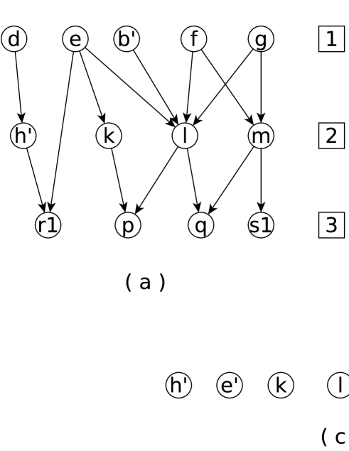
Figure 2: (a) 1-Compressed Graph $G^{1}$, (b) Modified 1-compressed Graph $G^{1}_{m}$, (c) 2-Compressed Graph $G^{2}$

Dummy edges data structure: We described earlier, we do not need to handle single-level edges separately. However if two continuous single-level edges are removed, we still need to maintain the logical connection between the even-topology vertices. For example, in Figure 1(a) edges $(e,i),(i,k)$, and $(i,l)$ are single-level edges which will be deleted after the first compression iteration because $topo(i)=3$. Now, information of logical (indirect) connection between $e$ to $k$ and $l$ needs to be maintained, because all three vertices will exist after the compression. To handle this, we add new dummy edges $(e,k)$ and $(e,l)$; dummy edges are shown as dotted lines in Figure 1(b). Note that, for any dummy edge $(u,v)$, $topo(v)-topo(u)=2$ in the current DAG and the edges for which the node-topology difference is higher than 2 are handled by the above 4 multi-level edge cases. For same start and end nodes, if there are multiple dummy edges, TopCom considers edge with the smallest distance. To find the dummy edges, we scan through all odd-topology vertices and find their single-level incoming and outgoing edges. We store all these dummy edges along with the corresponding distance value in a list called $DummyEdges$ as shown in Figure 1, which we use during the index generation step. For example dummy edge $(d,h^{\prime})$ has a distance 2 in the Figure 1, then $[(d,h^{\prime}),2]$ is stored in $DummyEdges$.

At each compression iteration, we first obtain a modified graph, with fictitious vertices, copied vertices, and dummy edges and then apply compression to obtain the compressed graph of the subsequent iteration. The fictitious vertices, copied vertices, and dummy edges of the modified graph in earlier iteration become regular vertices and edges of the compressed graph in subsequent iteration. The above modification and compression proceeds iteratively until we reach $t$-compressed graph, $G^{t}$, for which the topological level number is 1. We use $G_{m}$ to denote the modified uncompressed graph, $G^{1}_{m}$ to denote the modified 1-compressed graph, $G^{2}_{m}$ to denote the modified 2-compressed graph and so on. For example, Figure 2(a) shows $G^{1}$ which is obtained by compressing the modified graph $G_{m}$ in Figure 1(b). Figure 2(b) shows $G^{1}_{m}$, the modified 1-compressed graph, and Figure 2(c) shows $G^{2}$, the 2-compressed graph. We refer the set of all modified compressed graphs as $G^{*}_{m}$, i.e. $\{$ $G^{t}_{m},...,G^{2}_{m},G^{1}_{m}$ $\}$.

3.2 Index generation

TopCom’s index data structure is represented as a table of key-value pairs. For each key, (vertex) $v$ of the input graph, the value contains two lists: (i) outgoing index value $I^{out}_{v}$ , which stores shortest distances from $v$ to a set of vertices reachable from $v$; and (ii) incoming index value $I^{in}_{v}$, which stores shortest distances between $v$ and a set of vertices that can reach $v$. Both the lists contain a collection of tuples, $\langle vertex\_id,distance\rangle$, where vertex_id is the id of a vertex other than $v$, and distance is the corresponding shortest path distance between $v$ and that vertex.

Algorithm 1 Outgoing Index value Generation

0:  $G^{*}_{m}$ (set of modified graphs), DummyEdges (set of dummy edges and corresponding distance)

0:  $I^{out}_{*}$ (set of out going indexes for all nodes)

1:  for all $G^{curr}_{m}\in\{G^{topo(G)}_{m},...,G^{1}_{m},G_{m}\}$ do

2:     $O$ = $\{u\in V(G^{curr}_{m})|topo(u)=odd\_number\}$

3:     for all $v\in O$ do

4:        $org\_v$ = GetOriginal$(v)$

5:        for all $(v,w)\in{E(G^{curr}_{m})}$ do

6:           $org\_w$ = GetOriginal$(w)$

7:           if $org\_v==org\_w$ then

8:              Continue

9:           end if

10:           if $(v,w)==Dummy\_Edge$ then

11:              distance = GetDummyDistance$(DummyEdges,v,w)$

12:           end if

13:           if $w==fictitious\_vertex$ then

14:              distance = distance - 1

15:           end if

16:           RecursiveInsert$(I^{out}_{org\_v},org\_w,distance,out)$

17:        end for

18:     end for

19:  end for

At the beginning of the indexing step, for each vertex $v$, TopCom initializes $I^{out}_{v}$ and $I^{in}_{v}$ with an empty set. It generates index from $G^{t}_{m}$ and repeats the process in reverse order of graph compression i.e. from graph $G^{t}_{m}$ to $G_{m}$. In $i$’th iteration of index building, it uses $G^{t-i}_{m}$ and inserts a set of tuples in $I^{out}_{v}$ and $I^{in}_{v}$, only if $v$ is an odd-topology vertex in $G^{t-i}_{m}$. Thus, during the first iteration, for every odd-topology vertex $v$ of $G^{t-1}_{m}$, for an incoming edge $(u,v)$ TopCom first checks whether $(u,v)$ is in $DummyEdges$ data structure, if so, it inserts $\langle u,d\rangle$ in $I^{in}_{v}$, where the distance $d$ value is obtained from the $DummyEdges$ data structure. Otherwise, it inserts $\langle u,1\rangle$ in $I^{in}_{v}$. Similarly, for an outgoing edge $(v,w)$ TopCom inserts $\langle w,d\rangle$ in $I^{out}_{v}$, if $(v,w)$ is in $DummyEdges$, otherwise it inserts $\langle w,1\rangle$ in $I^{out}_{v}$. TopCom also inserts (Line 16 in Algorithm 1) elements of $I^{in}_{u}$ and $I^{out}_{w}$ into $I^{in}_{v}$ and $I^{out}_{v}$, respectively, using recursive calls.

Algorithm 1 shows the pseudo-code of the index generation procedure for outgoing index values only. An identical piece of code can be used for generating incoming index values also, but for that we need to exchange the roles of fictitious and copied vertex, and change the $I^{out}_{*}$ with $I^{in}_{*}$ in Line 5-21 (more discussion on this is forthcoming).

As shown in Line 2 of Algorithm 1, TopCom first collects all odd-topology vertices in variable $O$ and builds out-indexes for each of these vertices using outgoing edges from these vertices (the edge $(v,w)$ in Line 5 of Algorithm 1). Note that, vertices $v$ and $w$ in $G^{curr}_{m}$ can be fictitious or copied vertex; TopCom uses the subroutine GetOriginal() which returns original vertex corresponding to any fictitious or copied vertex, if necessary (Line 4 and 6). Using the data structure $DummyEdges$ (discussed in section 3.1), it first checks whether the edge $(v,w)$ is a dummy edge (Line 10); if so, it obtains the actual distance from the data structure. In case the end-vertex $w$ is a fictitious vertex, TopCom decrements the distance value by 1 (Line 14), because for each fictitious vertex, an extra edge with distance 1 is added from the original vertex to the fictitious vertex which has increased the distance value by one. For instance, in the graph in Figure 1, the actual distance from $a$ to $h$ is 2, but the fictitious vertex $h^{\prime}$ records the distance to be $3$, which should be corrected. On the other hand, if $w$ is a copied vertex, TopCom does not make this subtraction, because when a copied vertex is used as destination instead of the original vertex, the distance between the source vertex and the copied vertex correctly reflects the actual distance. For an example, in the same graph, the distance between $e$ and $r$ is 1; when we use the copied vertex $r1$ instead of $r$, distance between $e$ and $r1$ is recorded as 1, which is the correct distance between $e$ and $r$; so no distance correction is needed during the out index building when the destination vertex is a copied vertex. This is the reason why we make a distinction between the fictitious vertices and the copied vertices.

Finallly note that, after generating indexes for each vertex there may be multiple entries for some vertices; from these multiple entries we need to get the smallest value (entry) and remove others. For building incoming index values, TopCom subtracts 1 for a copied vertex, but does not subtract 1 for a fictitious vertex, as the roles of start and end vertices flip for the incoming index values. Below, we give a complete index building example using the vertex $a$ of the graph in Figure 1.

Table 1: Intermediate index generated from the DAG in Figure 2(b)

key	Out Index value	key	In Index value
b	$\{\langle l,1\rangle\}$	p	$\{\langle k,2\rangle,\langle l,2\rangle\}$
d	$\{\langle h,1\rangle\}$	q	$\{\langle m,1\rangle,\langle l,2\rangle\}$
e	$\{\langle k,2\rangle,\langle l,2\rangle\}$	r	$\{\langle h,1\rangle,\langle e,1\rangle\}$
f	$\{\langle l,2\rangle,\langle m,2\rangle\}$	s	$\{\langle m,1\rangle\}$
g	$\{\langle l,2\rangle,\langle m,2\rangle\}$

Table 2: Index for the DAG in Figure 1

key	Out Index value	In Index value
a	$\{\langle d,1\rangle,\langle e,1\rangle,\langle h,2\rangle,\langle k,3\rangle,\langle l,3\rangle\}$	$\emptyset$
b	$\{\langle l,1\rangle,\langle f,1\rangle,\langle m,3\rangle\}$	$\emptyset$
c	$\{\langle f,1\rangle,\langle g,1\rangle,\langle l,3\rangle,\langle m,3\rangle\}$	$\emptyset$
d	$\{\langle h,1\rangle\}$	$\emptyset$
e	$\{\langle k,2\rangle,\langle l,2\rangle\}$	$\emptyset$
f	$\{\langle l,2\rangle,\langle m,2\rangle\}$	$\emptyset$
g	$\{\langle l,2\rangle,\langle m,2\rangle\}$	$\emptyset$
h	$\emptyset$	$\{\langle d,1\rangle\}$
i	$\{\langle k,1\rangle,\langle l,1\rangle\}$	$\{\langle e,1\rangle\}$
j	$\{\langle l,1\rangle,\langle m,1\rangle\}$	$\{\langle f,1\rangle,\langle g,1\rangle\}$
n	$\{\langle p,1\rangle\}$	$\{\langle k,1\rangle\}$
o	$\{\langle p,1\rangle\}$	$\{\langle l,1\rangle\}$
p	$\emptyset$	$\{\langle k,2\rangle,\langle l,2\rangle\}$
q	$\emptyset$	$\{\langle m,1\rangle,\langle l,2\rangle\}$
r	$\emptyset$	$\{\langle h,1\rangle,\langle e,1),\langle p,1\rangle,\langle k,3\rangle,\langle l,3\rangle\}$
s	$\emptyset$	$\{\langle m,1\rangle,\langle p,1\rangle,\langle k,3\rangle,\langle l,3\rangle,\langle q,1\rangle\}$

Example: We want to find the outgoing index (value) for vertex $a$ (key) of the graph $G$ in Figure 1(a). $topo(G)=2$, so we start building index using the graph $G^{1}_{m}$, which is shown in Figure 2(b). In the first iteration, TopCom builds $I^{out}_{d}=\{\langle h,1\rangle\}$; the distance value of $1$ comes as follows: TopCom uses distance of dummy edge $(d,h^{\prime})$ that is 2 (Figure 1-II) and then it replaces the fictitious vertex $h^{\prime}$ with $h$ and obtains a distance of 1 by subtracting 1 from 2 (Line 14). It also inserts the following entries under the key $e$; i.e., $I^{out}_{e}=\{\langle k,2\rangle,\langle l,2\rangle\}$. The resulting indexes after this iteration is presented in Table 1; incoming index values for keys $b,d,e,f,g$ are empty (not presented in the table) and similarly outgoing index values for keys $p,q,r,s$ are empty. For next iteration considering $G_{m}$, TopCom inserts $\langle d,1\rangle$ in $I^{out}_{a}$; using recursive calls of algorithm 2 (Line 11), this function also inserts $\langle h,2\rangle$ in $I^{out}_{a}$, recursion stops at $h$ because $I^{out}_{h}$ is empty (Line 6). Similarly, $\langle e,1\rangle$ and $\langle k,3\rangle,\langle l,3\rangle$ are inserted in $I^{out}_{a}$ recursively from $I^{out}_{e}$. At the end of the algorithm 1 we remove duplicate entries from indexes. For example, incoming index for key $s$ has two entries for vertex $m$, $\langle m,1\rangle$ and $\langle m,2\rangle$, one corresponding to edge $(m,s1)$ in $G^{1}_{m}$ and the other is a recursive result from $q$ to $s$ in $G_{m}$. TopCom considers $\langle m,1\rangle$ and discards the other entry from $I^{in}_{s}$. For the graph in Figure 1(a), corresponding indexes are presented in Table 2.

Algorithm 2 RecursiveInsert$(I^{io}_{v},a,distance,in\_or\_out)$

1:  if $in\_or\_out==in$ then

2:     $I^{io}_{a}=I^{in}_{a}$

3:  else

4:     $I^{io}_{a}=I^{out}_{a}$

5:  end if

6:  if $I^{io}_{a}==\emptyset$ then

7:     $add\_tuple(I^{io}_{v},a,distance)$

8:  else

9:     $add\_tuple(I^{io}_{v},a,distance)$

10:     for all $(x,dist)\in I^{io}_{a}$ do

11:        RecursiveInsert$(I^{io}_{v},$ $x,$ $distance$ $+$ $dist,$ $in\_or\_out)$

12:     end for

13:  end if

3.3 Index for weighted graph

For weighted graph, TopCom makes some minor changes in the above algorithm. First, distance values are stored both in the indexes and in the $DummyEdge$ data structure. Many of these distances are implicitly 1 for unweighted graph, which is not true for weighted graph, so, for the latter TopCom stores the distance explicitly. Also, it ensures that the distance value between fictitious (or copied) vertices and an original vertex is one, so that the Algorithm 1 works as it is.

3.4 Query processing

For query processing, TopCom uses the distance indexes that is built during the indexing stage. For a given distance query from $u$ to $v$, i.e. to compute $\delta(u,v)$, TopCom intersects outgoing index value of key $u$ i.e. $I^{out}_{u}$ and incoming index value of key $v$ i.e. $I^{in}_{v}$ and finds common vertex_id in $I^{out}_{u}$ and $I^{in}_{v}$, along with the distance values. To cover the cases, when $v$ is in the outgoing index value of $u$, or $u$ is in the incoming index value of $v$, the tuples $\langle u,0\rangle$ and $\langle v,0\rangle$ are also added in $I^{out}_{u}$ and $I^{in}_{v}$ respectively and then the intersection set of the indexes is found. If the intersection set size is 0, there is no path from $u$ to $v$ and hence the distance is infinity. Otherwise, the distance is simply the sum of the distances from $u$ to vertex_id and vertex_id to $v$. If multiple paths exist, we take the one that has the smallest distance value.

Example: We want to find $\delta(a,s)$ in Figure 1. From table 2, $I^{out}_{a}\cap I^{in}_{s}=\{k,l\}$. Now, we need to sum up the corresponding distance values, that gives $\{\langle k,6\rangle,\langle l,6\rangle\}$. Now we need to find smallest distance value; in this case both the values are same, hence we can provide any one as a result.

3.5 Theoretical proofs for correctness

In this section, we prove the correctness of TopCom, through the claim that TopCom’s index is based on 2-hop covers of the shortest distance in a graph and method described in Section 3.4 gives correct shortest distance value. For shortest path, such a cover is a collection $S$ of shortest paths such that for every two vertices $u$ and $v$, there is a shortest path from $u$ to $v$ that is a concatenation of atmost two paths from $S$. [2Hop:Cohen:2002]. That is, shortest path from $u$ to $v$ is stored in $S$ or there is an intermediate node $x$ such that shortest paths from $u$ to $x$ and from $x$ to $v$ are stored in $S$. For TopCom’s index also, the shortest distance from any node $u$ to node $v$ is the 2-hop cover such that the index itself has shortest distance value from $u$ to $v$ or there is an intermediate node $x$ which would be present in both $I^{out}_{u}$ and $I^{in}_{v}$.

Example: In DAG $G$ in Figure 1(a) to find distance from $a$ to $s$, we need to check the outgoing index value for vertex $a$ and the incoming index value for vertex $s$ in Table 2. This gives us two possible shortest paths passing through intermediate node $k$ or $l$, because distance in both cases is same. Thus, there can be multiple shortest paths however, atmost one intermediate node in the index.

In the Theorem 3.5, we try to identify the topological layer of an intermediate node $x$. We identify a unique topological level for each pair of $u$ and $v$, which tells there is atmost one intermediate node in a shortest path from $u$ to $v$ because in DAG there cannot be a directed edge within topological layer. We begin with the following lemmas, which will be useful for constructing the proof of the theorem.

Lemma 3.1.

In $G_{m}$, if a node $u$ is at topological level $2^{i}$, it will be at topological level $1$ in $G^{i}$.

Proof 3.2.

Example In the graph $G_{m}$ shown in Figure 1(b), the node $d$ is at topological level $2$ and the node $k$ is at topological level $4$. In $G^{1}$ shown in Figure 2(a) the node $d$ is at topological level $1$; similarly, in $G^{2}$ shown in Figure 2(c), the node $k$ is at topological level $1$.

Lemma 3.3.

In

Proof 3.4.

As per Line 2 of Algorithm 1,

Example: See the completely built index of the graph $G$ in Figure 1(a) as shown in Table 2. The nodes that appear as values are $\{d,e,b^{\prime}(b),f,g,h^{\prime}(h),k,l,m,r_{1}(r),p,q,s_{1}(s)\}$. All of these are from the even topology nodes in $G_{m}$ as shown in Figure 1(b).

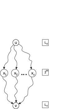
Figure 3: Shortest path from $u$ to $v$ passing through $x$

Theorem 3.5.

For finding shortest distance from $u$ to $v$, assume that $u$ has topological level number $L_{u}$ and $v$ has topological level number $L_{v}$ in $G_{m}$. We define

$$n=\arg\!\max_{i}(L_{u}\leq 2^{i}\leq L_{v})$$ (1)

Now, if there is a shortest path from $u$ to $v$, for each shortest path, exclusively, one of the following is true.

Case 1: No intermediate node $x$ i.e. $I^{out}_{u}$ includes $v$ or $I^{in}_{v}$ includes $u$.

Case 2: There is an intermediate node $x$, and

$$topo(x)=2^{n}+C$$

for some constant offset C.

Proof 3.6.

We prove this theorem using mathematical induction on $n$.

Base case: $n=1$. If there is a direct edge from $u$ to $v$ then case 1 is true because if $L_{u}=2$ then $I^{in}_{v}$ includes $u$ or if $L_{v}=2$ then $I^{out}_{u}$ includes $v$. If there is an intermediate node $x$ then $L_{u}=1$ and $L_{v}=3$, hence $topo(x)=2$ that shows case 2 is true. From Lemma 3.3 both $I^{out}_{u}$ and $I^{in}_{v}$ include the node $x$ if there is a path from $u$ to $v$. In this case constant offset C would be zero.

Induction hypothesis: Here we assume that for $n=d$ given theorem is true.

Induction step: We want to prove, for $n=d+1$ given theorem is true.

If there is no intermediate node $x$ then case 1 is true. Hence, we discuss the only scenario where there is an intermediate node $x$ and we want to show that $x$ is in both $I^{out}_{u}$ and $I^{in}_{v}$. We sub-divide the proof for zero and non-zero values of constant offset C.

Constant offset C is zero:

If there are $2^{d+1}$ levels, then compression step would be conducted at least one more time than $2^{d}$ levels. From Lemma 3.1 at the $d$’th step of compression, nodes at topological level $2^{d}$ in graph $G_{m}$ are at $1^{st}$ topological level in $G^{d}$ and nodes from topological level $2^{d+1}$ would be at $2^{nd}$ topological level.

Hence,

Example of non-zero offset C: In Figure 1(b), we want to know the shortest distance from $n$ to $r$ where corresponding topological levels are $L_{n}=5$ and $L_{r}=7$ respectively. For this, we can not find any $n$ that satisfies the equation 1. From equation LABEL:eq2, we can calculate $n_{low}=2$, using which modified topological levels $L^{m}_{n}=1(5-2^{2})$ and $L^{m}_{r}=3$ can be obtained. From $L^{m}_{n}$ and $L^{m}_{r}$ we get $m=1$. Now, $2^{1}+2^{2}=6$ is the topological level of intermediate node $p$, which is present in both $I^{out}_{n}$ and $I^{in}_{r}$ (Table 2). If we look carefully $L^{m}_{n}$ and $L^{m}_{r}$ is a base case in the mathematical induction proof of Theorem 3.5, and $L_{n}(5)$, $L_{r}(7)$ with offset C behave exactly the same as the base case.

Note: If there is no node from topological level $2^{n}$ in the shortest path from $u$ to $v$, then there must be one multilevel edge which skips that level. For a node incident to that multilevel edge, at some step of the compression, we need to prepare fictitious/copied node. That new fictitious/copied node works as a node from topological level $2^{n}$ and will be included in both $I^{out}_{u}$ and $I^{in}_{v}$. Thus, theorem works fine for this case.

For example, as depicted in Figure 1(b), shortest path from $a$ to $r$ doesn’t pass through any node from topological level $4(2^{2})$ in $G_{m}$, but it has a multilevel edge $(e,r_{1})$. In $G^{2}_{m}$ (Figure 2(b)), this edge causes a fictitious node $e^{\prime}$ at topological level $2$ which is (logically) topological level $4$ in $G_{m}$. The resulting index in Table 2 shows that, the node $e^{\prime}(e)$ is included as a value in the incoming index of $r$ ($I^{in}_{r}$) and also included in $I^{out}_{a}$.

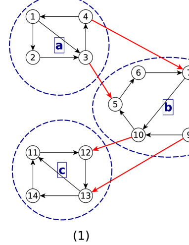
(a) (1)Example for Distance within Middle DAG node of $G_{d}$ and (2)Example of multiple dummy edges in modified $G_{d}$

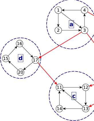
(b) Example of merging multiple dummy DAG edges

Figure 4: Dummy edge handling

4 Indexing for general directed graph

Any directed graph $G$ can be converted to a Directed Acyclic Graph (DAG) $G_{d}$, by considering each strongly connected component (SCC) of $G$ as a node of $G_{d}$. Thus in DAG, the edges within a SCC are collapsed within the corresponding node. However, if an edge in $G$ connects two vertices from two distinct SCCs, in $G_{d}$ those SCCs are connected by a DAG edge. To build the shortest path index for a general directed graph,

Algorithm 5.

first uses Tarjan’s algorithm [DFS:Tarjan:1972] to convert $G$ to a DAG $G_{d}$ by finding all SCCs of $G$. It also maintains a necessary data structure that keeps the mapping from a DAG node to a set of graph vertices, and vice-versa. We call this a parent-child mapping, i.e., a DAG node is the parent of graph vertices which are part of the corresponding SCC. A DAG edge connects two vertices, one from a distinct SCC. We call such vertices terminal vertices. A single DAG edge between a pair of SCCs may encapsulate multiple paths (one edge or multiple edges) of Graph $G$ such that the end vertices of these paths are terminal vertices in those pair of SCCs.