Nematic quantum phase transition of composite Fermi liquids in half-filled Landau levels and their geometric response

Abstract

We present a theory of the isotropic-nematic quantum phase transition in the composite Fermi liquid arising in half-filled Landau levels. We show that the quantum phase transition between the isotropic and the nematic phase is triggered by an attractive quadrupolar interaction between electrons, as in the case of conventional Fermi liquids. We derive the theory of the nematic state and of the phase transition. This theory is based on the flux attachment procedure which maps an electron liquid in half-filled Landau levels into the composite Fermi liquid close to a nematic transition. We show that the local fluctuations of the nematic order parameters act as an effective dynamical metric interplaying with the underlying Chern-Simons gauge fields associated with the flux attachment. Both the fluctuations of the Chern-Simons gauge field and the nematic order parameter can destroy the composite fermion quasiparticles and drive the system into a non-Fermi liquid state. The effective field theory for the isotropic-nematic phase transition is shown to have $z=3$ dynamical exponent due to the Landau damping of the dense Fermi system. We show that there is a Berry phase type term which governs the effective dynamics of the nematic order parameter fluctuations, which can be interpreted as a non-universal “Hall viscosity” of the dynamical metric. We also show that the effective field theory of this compressible fluid has a Wen-Zee-type term. Both terms originate from the time-reversal breaking fluctuation of the Chern-Simons gauge fields. We present a perturbative (one-loop) computation of the Hall viscosity and also show that this term is also obtained by a Ward identity. We show that the topological excitation of the nematic fluid, the disclination, carries an electric charge. We show that a resonance observed in radio-frequency conductivity experiments can be interpreted as a Goldstone nematic mode gapped by lattice effects.

I Introduction and Motivation

Electronic nematic phases have been a focus of attention during the past few years in several areas of quantum condensed matter physics.Fradkin et al. (2010) An electronic nematic is a state of a strongly correlated electronic system in which rotational invariance is broken spontaneously without breaking translation symmetry. Unlike their classical liquid crystal cousins,Chaikin and Lubensky (1995); de Gennes and Prost (1993) whose tendency to exhibit orientational order can be traced back to the microscopic cigar-shaped nature of the constituent nematogen molecules, an electronic nematic phase arises from the self-organization of electrons in a strongly correlated material.

The electronic nematic state belongs to a class of phases of strongly-interacting quantum-mechanical electronic matter, known as electronic liquid crystal states,Kivelson et al. (1998); Fradkin and Kivelson (1999) which are characterized by the spontaneous breaking of the spatial symmetries of a physical system. Electronic nematic phases have by now been discovered experimentally in many different systems ranging, among others, from high temperature cuprate superconductors, such as in YBa₂Cu₃O_6+xAndo et al. (2002); Hinkov et al. (2008); Daou et al. (2010) for a broad range of doping levels, and in underdoped Bi₂Sr₂CaCu₂O_8+δ,Lawler et al. (2010) to iron-based superconductors such as Ca(Fe_1-xCo_x)₂As₂,Chu et al. (2012) and also to the bilayer ruthenate Sr₃Ru₂O₇.Borzi et al. (2007)

However, the first and to this date the most spectacular experimental evidence for an electronic nematic state was discovered in two-dimensional electron gases (2DEG) in high magnetic fields in the middle of the second, $N=2$, Landau level (and higher), in regimes in which the 2DEG is compressible and the fractional quantum Hall (FQH) effect is not observed.Lilly et al. (1999a); Du et al. (1999) In these experiments, longitudinal and Hall transport measurements were made in the center of the Landau level for Landau levels $N\geq 2$. It was found that the longitudinal transport properties exhibit a strong spatial anisotropy (with a ratio of resistances as large as 3,500 in the cleanest samples at the lowest temperatures, originally down to $T\gtrsim 25$ mK). This anisotropy has a fairly rapid increase at a temperature $T\simeq 65$ mK from a nominal anisotropy of a fraction of a percent at $T\sim 1$ K. Importantly, in this regime the I-V curves are linear at low bias and, hence, do not show any signs of translation symmetry breaking, e.g. no threshold electric fields, characteristic for a charge-density-wave ground state, were ever detected in this regime. In contrast, in the same samples and at the same temperatures, a reentrant integer quantum Hall plateau is observed away from the center of the Landau level, and, in this regime, an extremely sharp threshold electric field is seen, with a sharp onset of narrow-band noise for larger electric fields.Cooper et al. (2002, 2003); Fradkin et al. (2010) Nevertheless, these experiments were originally interpreted as evidence of a striped ground state, an interpretation still used in the literature.

Hence, in the compressible anisotropic regime, down to the lowest temperature accessible in the experiments (which currently go down to about $10$ mK), the 2DEG behaves as a compressible charged fluid with a large anisotropy which onsets below a well defined temperature. This behavior strongly suggested that there is a (thermal) phase transition of the 2DEG, rounded by a very weak native anisotropy (with a characteristic energy scale estimated to be $\sim 3-5$ mK, whose microscopic origin has remained unclearPollanen et al. (2015)) to a low-temperature electronic nematic state.Fradkin and Kivelson (1999) The nematic nature of the state was verified by detailed fits of the transport anisotropy data to classical Monte Carlo simulations of the thermal fluctuations of nematic order.Fradkin et al. (2000); Cooper et al. (2001)

Subsequent experiments in 2DEGs in quantum wells, earlier by tilting the magnetic field,Lilly et al. (1999b); Pan et al. (1999) and, more recently, by the application of hydrostatic pressure in the absence of an in-plane magnetic field,Samkharadze et al. (2016) have revealed the existence of a complex phase diagram in which compressible nematic phases were found even in the first Landau level, $N=1$, competing with the famous, presumably non-Abelian, paired, FQH state at filling fraction $\nu=5/2$. More recent tilted field experiments have also revealed the existence of an incompressible nematic FQH state in the $N=1$ Landau level at filling fraction $\nu=7/3$, competing with the isotropic Laughlin-like FQH state at that filling fraction.Xia et al. (2010, 2011) No nematic state has ever been reported in the lowest, $N=0$, Landau level.

Early Hartree-Fock theories of the 2DEGs near the center of the Landau level, for Landau level index $N$ large enough, have predicted a stripe-like ground state, i.e. a compressible state in which the electron density is spontaneously modulated along one direction.Moessner and Chalker (1996); Koulakov et al. (1996); Fogler et al. (1996) For this reason, the anisotropic states in the compressible regimes in Landau levels $N\geq 2$ were originally referred to as striped states. Most microscopic theories for the anisotropic state at $\nu=9/2$ (and in higher Landau levels) were built on this proposal.MacDonald and M. P. A. Fisher (2000); Stanescu et al. (2000); Barci et al. (2002); Fogler (2002); Côté and Fertig (2000); Lopatnikova et al. (2001); Lawler and Fradkin (2004) The resulting picture of the stripe state is an array of “sliding” Luttinger liquids.Emery et al. (2000); Vishwanath and Carpentier (2001); Sondhi and Yang (2001); Fertig (1999)

On the other hand, an exact diagonalization study by Rezayi and HaldaneRezayi and Haldane (2000) for a system of up to 16 electrons for half-filled Landau levels in a toroidal geometry gave strong evidence for both a paired FQH state and a stripe-like state as a function of the effective interactions in the Landau level. We should note that in such small system (and in a toroidal geometry) finite-size effects can blur the distinction between a stripe state and a nematic state, but it is an evidence for at least short-range stripe order.

Interest in nematic quantum Hall states attracted renewed attention after the experimental discovery of an incompressible nematic phase inside the fractional quantum Hall state in the $N=1$ Landau level at filling fraction $\nu=7/3$ by Xia and coworkers.Xia et al. (2010, 2011) This state has been studied theoretically by several groups.Mulligan et al. (2010); You and Fradkin (2013); You et al. (2014); Haldane (2009, 2011); Yang (2013); Maciejko et al. (2013) These studies have revealed that nematic fluctuations are intimately related to the geometric response of the quantum Hall fluid and, in particular, to the Hall viscosity. The incompressible nature of nematic fractional quantum Hall states strongly constrains the behavior of the nematic fluctuations and largely determines the structure of the effective behavior at low energies. These studies have also shown that the nematic transition inside the FQH state is triggered by a softening and condensation of the stable collective mode of the FQH fluid, the Girvin-MacDonald-Platzman (GMP) mode, at zero momentum.

The close vicinity of nematic order of a compressible state or a FQH state (which is hence incompressible) strongly suggests that the nature of the effective interactions in the 2DEG in Landau levels $N\geq 1$ favor both paired and nematic ordered states. In this context, it is surprising that, in spite of all the work on nematicity in the incompressible state, there has been almost no work on the compressible nematic state for more than a decade. Aside from the notable semi-phenomenological theory of the quantum Hall nematic of Radzihovsky and Dorsey,Radzihovsky and Dorsey (2002) based both on a microscopic theory and on quantum hydrodynamics, and of the work of Wexler and Dorsey,Wexler and Dorsey (2001) who made estimates of the dislocation-unbinding transition of a quantum Hall stripe state to a quantum Hall nematic based on the Hartree-Fock theory of the stripe state, except for a variational Monte Carlo wave function study by Doan and Manousakis,Doan and Manousakis (2007) the compressible nematic state has not been studied.

In principle there are two logical pathways to reach a nematic phase by a quantum phase transition: a) by quantum melting of a stripe phase, or b) by a (Pomeranchuk) instability of an isotropic Fermi liquid type state. Although the close vicinity of the isotropic compressible Fermi liquid state to the observed nematic state in Landau levels $N\geq 1$ suggests that the latter may be a suitable starting point, the fact that exact diagonalization studies find local stripe orderRezayi and Haldane (2000) suggests that the actual physics is likely to lie somewhere in between these two regimes. Also, it is possible that the state is nematic above some critical temperature while the ground state may be a stripe phase. However, the fact that there is strong evidence for rotation symmetry breaking but not of translation symmetry breaking, down to the lowest experimentally accessible temperatures, suggests that the ground state may be a nematic state (perhaps close to a quantum phase transition to a stripe phase.)

The purpose of this paper is to develop a theory of the compressible nematic state of the 2DEG in large magnetic fields. Throughout this work we will use the mapping of electrons in Landau levels to composite fermions in the same Landau levels but now coupled to a Chern-Simons gauge field,López and Fradkin (1991); Fradkin (2013) i.e. a flux attachment transformation. At a formal first-quantized level this mapping is an exact identity. However the resulting theory has no small parameter and in practice a mean field theory, the average field approximation, must be used. For FQH states, which have a finite energy gap already at the level of the mean field theory, this approach has been shown to yield exact predictions of the universal properties of the fractional quantum Hall fluid, including the Hall conductance, the charge and statistics of the excitations, degeneracy on a torus, and the Hall viscosity and related geometric responses.Fradkin (2013); Cho et al. (2014); Gromov et al. (2015) On the other hand, here we will be interested in compressible phases which do not have a gap (by definition) and hence the theory is not as well controlled as in the FQH regime. As our starting point we will consider the isotropic Fermi liquid state of Halperin, Lee and ReadHalperin et al. (1993); Read (1994) (HLR) of composite fermions,Jain (1989) which is based on the same mapping, and look for a Pomeranchuk quantum phase transition to a nematic state. This is a natural point of view which has been used extensively as a description of nematic Fermi fluids.Oganesyan et al. (2001) However, the HLR Fermi liquid is a non-Fermi liquid to begin with which makes the application of these ideas not straightforward.

At the level of mean field theory, the HLR (or Jain) Fermi liquid states are the limiting state of the FQH states in the Jain sequencesJain (1989) with filling fraction $\nu=p/(2np\pm 1)$, where $p$ and $n$ are two non-negative integers. In Jain’s picture, a FQH state of electrons can be viewed (in mean field theory) as an integer quantum Hall state with filling fraction $\pm p$ of composite fermions, which is made of gluing $2n$ fluxes to every electron, in a partially screened magnetic field $B/(2np\pm 1)$. In the compressible limit, $|p|\to\infty$, the effective magnetic field felt by the composite fermions vanishes (on average) or, equivalently, the effective charge of the fermions vanishes in the same limit. In this regime, the charge-neutral composite fermions fill a Fermi sea and form a (composite) Fermi liquid.Jain (1992) This simple picture, and its subsequent extensions, has given a successful description of numerous experiments in the compressible regime.Willett et al. (1990); Kang et al. (1993); Goldman et al. (1994); Jain (2007) Also, a current picture of the microscopic origin of the non-abelian paired state in the first, $N=1$, Landau level, at filling fraction $\nu=5/2$, is a paired state in the $p_{x}+ip_{y}$ channel of composite fermions.Park et al. (1998); Read and Green (2000) It is then natural to look for a similar quantum transition to a compressible nematic state from the HLR state.

In Ref. [You et al., 2014] we worked out a theory of the incompressible nematic state in a fractional quantum Hall state using the flux attachment via fermion Chern-Simons gauge theoryLópez and Fradkin (1991) as a quantum phase transition in a Laughlin FQH state. Much as in the case of the nematic transition in a conventional Fermi liquid,Oganesyan et al. (2001) we showed that the quantum phase transition (the Pomeranchuk instability) can be caused by an effective quadrupolar interaction of among the electrons if it becomes sufficiently attractive. Furthermore, we showed that the electrons feel fluctuations of the nematic order parameter as an effective dynamical metric field. A direct consequence of this coupling is that the effective Lagrangian of the nematic fluctuations has a time-reversal breaking parity-odd Berry phase term, which is closely related to (but not equal to) the Hall viscosity. Due to this parity odd term, the quantum critical theory has dynamical exponent $z=2$. There are also Wen-Zee-like term in terms of the “effective” dynamical metric, i.e., nematic order parameters. In the nematic phase, there is a topological soliton, the nematic disclination, which in this fluid carries an (unquantized) electrical charge. The resulting effective field theory of the nematic fractional quantum Hall state obtained by this approach has the same structure and properties as the one proposed on symmetry grounds by Maciejko and coworkers.Maciejko et al. (2013)

The theory of the compressible nematic state that we will present here is naturally connected to our earlier work on the incompressible nematic FQH state. Thus, we will represent the problem of the half-filled Landau level and, in fact, for all the compressible limiting states of the Jain sequences, at filling fraction $\nu=1/(2n)$, as a system of composite fermions minimally coupled (i.e. in gauge-invariant way) to both the external electromagnetic field $A_{\mu}$ and to the statistical gauge field $a_{\mu}$ which implements the flux attachment. Hence, here too, the action also includes a Chern-Simons term (with a suitable coefficient).

Also, in addition to the Coulomb interaction, which only involves a coupling of the local densities, as in the case of a Fermi liquid,Oganesyan et al. (2001) we will also include an attractive interaction in the quadrupolar channel, i.e. an attractive interaction between the nematic densities. The coupling constant of this quadrupolar interaction is nothing but the $F_{2}$ Landau parameter of a Fermi liquid. By gauge invariance, the quadrupolar coupling of the fermions also involves both the gauge fields, $A_{\mu}$ and $a_{\mu}$, since the nematic densities are bilinear of the Fermi fields which necessarily involve spatial derivatives.

We will not attempt here to provide a microscopic derivation of the value (and sign) of the effective quadrupolar interaction. Nevertheless, it is well known that the effective interactions of composite fermions are quite different than those of electrons,Jain (2007) and depend on the Landau level index, as well as on properties of the heterostructure (or quantum well) which define the 2DEG. In addition, the estimate of values of Landau parameters, which is notoriously difficult even for conventional Fermi liquids, is much harder in the case of composite fermions. The currently available numerical estimatesLee et al. (2015) for $F_{2}$ obtain values that for $N\geq 1$ are very close to $-1$.

However, the physics of the compressible state is actually quite different from the FQH states, and the extension of this theory to the compressible state involves several problems. One is the lack of a small expansion parameter to control the theory. In the incompressible FQH states this is not a serious problem provided that one focused only on the long distance and low energy regime where it behaves as a topological fluid. This simplification is absent in the compressible state since it is gapless. Even though at the level of mean field theory the state is predicted to be a Fermi liquid, the coupling of the fluctuations of the statistical gauge field turns the (mean-field) HLR state into a non-Fermi liquid. Thus, already at the leading perturbative order, imaginary part of the the composite fermion self-energy $\Sigma^{\prime\prime}(\omega)$ overwhelms the real part,Halperin et al. (1993); Nayak and Wilczek (1994) i.e. $\Sigma^{\prime\prime}(\omega)\propto|\omega|^{2/3}$ for short-range interactions although it is milder for Coulomb interactions, $\Sigma^{\prime\prime}(\omega)\propto|\omega|$ ( a “marginal” Fermi liquid), and the composite fermion quasiparticles become ill-defined. In addition, a calculation of the Landau parameters $F_{l}$ for the HLR theoryStern and Halperin (1995) revealed that, for all angular momentum channels $l\geq 1$, all the Landau parameters are equal to the Pomeranchuk value, $F_{l}=-1$. Therefore, the quasiparticle picture breaks down and even the relic of a Fermi surface appears to be prone to instabilities (such as a nematic instability). Current numerical estimates in the half-filled Landau level yield negative values of $F_{2}$ and close to the Pomeranchuk instability value.Lee et al. (2015) Already the conventional theory of the nematic transition is non-trivial since at the Pomeranchuk point the Fermi liquid breaks down, and in the HLR state the Fermi liquid picture has been already broken down due to the coupling to the fluctuating gauge field. Nevertheless, properties of the fluid determined by gauge-invariant currents and densities are well behaved, in the sense that they are free of infrared singularities, although the results are at best qualitative since the theory does not have a small parameter.Kim et al. (1994); Shankar and Murthy (1997)

A further complication is the lack of particle-hole symmetry in the HLR theory.Kivelson et al. (1997) This problem is the focus of intense current work.Son (2015); Barkeshli et al. (2015); Wang and Senthil (2015); Geraedts et al. (2016); Metlitski and Vishwanath (2015); Kachru et al. (2015); Mulligan et al. (2016); Mross et al. (2015); Murthy and Shankar (2016) It has also been a focus of attention in the theory of the paired (Pfaffian) FQH state.Lee et al. (2007); Levin et al. (2007) Particle-hole symmetry in the half-filled Landau level can exist only in the absence of Landau level mixing and if only quadratic interactions are allowed. On the other hand, although the flux attachment transformation is an exact mapping, at the level of the average field approximation there is a large reorganization of the Hilbert space which involves a large mixing of Landau levels. For this reason the Jain wave functions are projected onto the Landau level. However, in the field theory approach there is no such projection.

In the incompressible FQH states the effects of Landau level mixing become negligible at long distances and at low energies provided that the quantum fluctuations (“one-loop” or “RPA”) are included, as a consequence of incompressibility, Galilean and gauge invariance.López and Fradkin (1992, 1993) The correct universal properties, encoded in the effective topological field theory, of the FQH states are reproduced only after these leading quantum corrections are included. These quantum corrections at long distance and at low energies turn the composite fermions into anyons with fractional charge and fractional statistics and, in this sense, there are no composite fermions in the spectrum of states of the FQH fluids. On the other hand, because of the absence of a small parameter, the theory yields quantitatively incorrect values for dimensionful (and non-universal) quantities, often by significant amounts although improvements have been made.Shankar and Murthy (1997) These problems become more complex in the case of the HLR state and, for this reason, theories of the compressible state projected onto the Landau level have been introduced.Pasquier and Haldane (1998); Read (1998) These theories are technically more complex and non-local, and are only qualitatively understood.

In what follows we will set aside these important caveats, and develop a theory of the compressible nematic state as an instability of the HLR composite Fermi liquid (CFL) state. In Section II we present the theory of the nematic composite Fermi liquid, following closely the structure and results of the theory of the nematic Fermi fluid of Oganesyan, Kivelson and Fradkin,Oganesyan et al. (2001) and of the composite Fermi liquid of Halperin, Lee and ReadHalperin et al. (1993) Here we introduce the gauge-invariant quadrupolar interaction, and present the basic structure of the effective action for the nematic order parameter fields. In Section III we derive the parity-even part of the nematic fluctuations, and in Section IV we derive the parity-odd component which yields the Hall viscosity using a diagrammatic approach. In Section V we derive a set of important Ward identities which we use throughout the paper. In Section VI we discuss the effective quantum dynamics of the nematic fields and their electromagnetic response which is relevant to resonance experiments. In Section VII we derive the Wen-Zee term for the CFL. Here we find that, due to the non-local nature of this term in the compressible state, not only its coefficient is not quantized (as it is in the incompressible FQH stateYou et al. (2014)) but its relation with the Berry phase term for the nematic fields (i.e. the effective Hall viscosity of the CFL) is not straightforward. In Section VIII we derive the geometrical response of the CFL and in particular the Hall viscosity of this compressible fluid. Here too, contrary to what happens in the FQH states, this response is not quantized and it is not universal. In Section IX, we discuss the connection of our theoretical results on the nematic CFL states with various experiments showing transport anisotropy in half-filled Landau levels. Section X is devoted to our conclusions and open questions. Details of our calculations and of previous results are presented in the Appendices. In Appendix A we give a summary of the theory of the quantum phase transition to a nematic state in a Fermi liquid of Oganesyan and coworkers,Oganesyan et al. (2001) and in Appendix B we summarize the HLR theory of the half-filled Landau level.Halperin et al. (1993) Details of the derivation of the Berry-phase-type term for the nematic fields are given in Appendix D and for the Wen-Zee term for the nematic fields in Appendix E. The derivation of the nematic correlators is given in Appendix F, and the vertex correction for the nematic polarization in Appendix G.

II Theory of Nematic Phase Transition of the Composite Fermi liquid

In this Section we consider the nematic-isotropic quantum phase transition inside the CFL. We will construct the theory using the theory of the nematic transition in a Fermi liquid of Oganesyan, Kivelson and FradkinOganesyan et al. (2001) (OFK), summarized in Appendix A, and the theory of the isotropic CFL of Halperin, Lee and Read,Halperin et al. (1993); Read (1994); Rezayi and Read (1994); Kim and Wen (1994) summarized in Appendix B, as our starting points.

Our starting point is the action for electrons in a half-filled Landau level of HLR with a quadrupolar interaction

$$\mathcal{S} =\int dtd^{2}r\Psi^{\dagger}(\bm{r},t)\Big{[}iD_{t}+\frac{\bm{D}^{2}}{2m}+\mu\Big{]}\Psi(\bm{r},t),$$

$$-\frac{1}{2}\int dtd^{2}rd^{2}r^{\prime}~{}V(\bm{r}-\bm{r}^{\prime})\delta\rho(\bm{r},t)\delta\rho(\bm{r}^{\prime},t)$$

$$-\frac{1}{2}\int dtd^{2}rd^{2}r^{\prime}~{}F_{2}(\bm{r}-\bm{r}^{\prime})\text{Tr}\Big{(}\hat{Q}(\bm{r},t)\cdot\hat{Q}(\bm{r}^{\prime},t)\Big{)},$$ (1)

where $D_{\mu}=\partial_{\mu}+iA_{\mu}$ is the covariant derivative and the index $\mu=t,x,y$ (not to be confused with the chemical potential which is also denoted by $\mu$!). Here $V({\bm{r}}-{\bm{r}}^{\prime})$ is the pair interaction potential, and the quadrupolar interaction $F_{2}$ in momentum space is represented as

$$F_{2}(\bm{q})=\frac{F_{2}}{1+\kappa\bm{q}^{2}}$$ (2)

Here we will use the same prescription we used in Ref.[You et al., 2014] in the context of the nematic FQH state, and we will be careful to include the gauge field $A_{\mu}$ in the definition of the nematic order parameter, the traceless symmetric tensor $\hat{Q}(\bm{r})$,

$$\hat{Q}(\bm{r})=\frac{1}{2m}\Psi^{\dagger}(\bm{r})\begin{pmatrix}D_{x}^{2}-D_{y}^{2}&2D_{x}D_{y}\\ 2D_{x}D_{y}&D_{y}^{2}-D_{x}^{2}\end{pmatrix}\Psi(\bm{r}),$$ (3)

where $D_{x}$ and $D_{y}$ are the $x$ and $y$ components of the covariant derivative which is explicitly dependent on the gauge field $A_{\mu}$. Hence, the nematic order parameter couples to the electromagnetic gauge field as a quadrupole.You et al. (2014)

II.1 Flux attachment and nematic order

Now we proceed to attach the flux using the Chern-Simons term and follow the same strategy as in the conventional CFL theory of Appendix B to find the following effective theory. In addition to this, we perform a Hubbard-Stratonovich transformation to decouple the quadrupolar interaction in terms of a field ${\bm{M}}({\bm{r}},t)=(M_{1}({\bm{r}},t),M_{2}({\bm{r}},t))$ (see also Appendix A), to find an action of the form

$$\mathcal{S} =\int dtd^{2}r\Psi^{\dagger}(\bm{r},t)\Big{[}iD_{t}+\frac{\bm{D}^{2}}{2m}+\mu+\alpha\bm{D}^{4}\Big{]}\Psi(\bm{r},t)-\frac{1}{2}\int d^{2}rd^{2}r^{\prime}dt\frac{1}{16\pi^{2}}\delta b({\bm{r}},t)V({\bm{r}-r^{\prime}})\delta b({\bm{r}^{\prime}},t)$$

$$+\int dtd^{2}r\frac{\varepsilon^{\mu\nu\lambda}}{8\pi}(\delta a_{\mu}-\delta A_{\mu})\partial_{\nu}(\delta a_{\lambda}-\delta A_{\lambda})+\int dtd^{2}r\Big{[}\frac{M_{1}}{2m}\Psi^{\dagger}(\bm{r},t)(D_{x}^{2}-D_{y}^{2})\Psi(\bm{r},t)+\frac{M_{2}}{2m}\Psi^{\dagger}(\bm{r},t)(2D_{x}D_{y})\Psi(\bm{r},t)\Big{]}$$

$$-\int dtd^{2}r\frac{1}{2F_{2}}\Big{[}\bm{M}^{2}+\kappa\left({\bm{\nabla}}{\bm{M}}\right)^{2}\Big{]}$$ (4)

where the covariant derivative now is $D_{\mu}=\partial_{\mu}+i\delta a_{\mu}$, where $\delta a_{\mu}$ is the fluctuating component of the Chern-Simons gauge field (See Appendix B), and where we have used the Chern-Simons constraint to replace the density fluctuation $\delta\rho({\bm{r}},t)$ with the Chern-Simons flux fluctuation $\delta b({\rm r},t)$ (as shown in Appendix B.)

The action of Eq.(4) is the theory that we will analyze in this paper. This action now also contains a higher-order gradient term, $\alpha\bm{D}^{4}$, in the fermion dispersion needed to stabilize the nematic phase, i.e., making the sign of the quartic term of the free energy of the nematic order parameter positive.Oganesyan et al. (2001) However, we will be mainly interested in the leading scaling behaviors of the various correlators in $\bm{q}$ and $\omega$ for small $q\ll k_{F}$ where we linearize the kinetic energy of the fermion near $k_{F}$ to calculate the correlators. Then the higher-order dispersion does not affect the leading scaling behaviors of the dynamic properties of the correlators. Therefore, from here and on, for the most part we we will drop the $\alpha\bm{D}^{4}$ term when calculating the dynamical properties of the CFL. We note that in our earlier work on the nematic fractional quantum Hall statesYou et al. (2014) it was necessary to include a term of order ${\bm{D}}^{6}$ to stabilize the nematic state, whereas here, in the compressible case, a term of order ${\bm{D}}^{4}$ is sufficient.

Our goal in this paper is to derive the effective theory for the external electromagnetic gauge field $\delta A_{\mu}$ and for the nematic order parameters $\bm{M}$. In this section we will sketch the calculation and highlight the important features of the results. The derivations of the main results are presented in the following Sections and in the Appendices.

We will proceed in two stages. First we will expand the effective action resulting from integrating out the fermions about the isotropic HLR state. The result is an effective action that depends also on the fluctuating piece of the Chern-Simons gauge field $\delta a_{\mu}$ (as it is done in Appendix B for the HLR theory). After integrating out the composite fermions we obtain the following effective action

$$\mathcal{S}_{\rm eff}[\delta a_{\mu},{\bm{M}},\delta A_{\mu}]= -i\textrm{tr}\ln\Big{[}iD_{t}+\frac{{\bm{D}}^{2}}{2m}+\mu+\alpha{\bm{D}}^{4}$$

$$+\frac{M_{1}}{2m}\left(D_{x}^{2}-D_{y}^{2}\right)+\frac{M_{2}}{2m}2D_{x}D_{y}\Big{]}$$

$$+\int d^{2}rdt \frac{1}{8\pi}\varepsilon^{\mu\nu\lambda}\left(\delta a_{\mu}-\delta A_{\mu}\right)\partial_{\nu}\left(\delta a_{\lambda}-\delta A_{\lambda}\right)$$

$$-\frac{1}{2}\int d^{2}rd^{2} r^{\prime}dt\frac{1}{16\pi^{2}}\delta b({\bm{r}},t)V({\bm{r}-r^{\prime}})\delta b({\bm{r}^{\prime}},t)$$

$$- \int d^{2}rdt\frac{1}{2F_{2}}\left[{\bm{M}}^{2}+\kappa\left({\bm{\nabla}}{\bm{M}}\right)^{2}\right]$$ (5)

Since we are interested in deriving an effective field theory near the nematic (Pomeranchuk) quantum phase transition, we will expand the fermion determinant (the first two lines on the right hand side of this effective action) up to the quartic order in the nematic fields $\bm{M}$ (and quadratic orders in their spatial derivatives). We will also expand the effective action up to the quadratic order in the fluctuations of the Chern-Simons gauge field $\delta a_{\mu}$. Notice that the only trace of broken time reversal invariance in this effective action is in the Chern-Simons action (the third line of this effective action), and that the fermion determinant represents a system of composite fermions at finite density (the HLR composite Fermi liquid) coupled to the fluctuations of the Chern-Simons gauge fields $\delta a_{\mu}$ and to the nematic fluctuations $\bm{M}$.

The result of this expansion is an effective action for the nematic fields $\bm{M}$ and an effective action for the fluctuations of the Chern-Simons gauge fields $\delta a_{\mu}$. The effective action has the general form

$$\mathcal{S}[\bm{M},\delta a_{\mu},\delta A_{\mu}]= \mathcal{S}_{n}[\bm{M}]+\mathcal{S}_{\textrm{CFL}}[\delta a_{\mu},A_{\mu}]$$

$$+ \mathcal{S}_{a,M}[\delta a_{\mu},\bm{M}]+\mathcal{S}_{a,M,a}[\delta a_{\mu},\bm{M}]$$ (6)

The first two terms of the right hand side are the expected terms for the effective action for nematic fields alone, $S_{n}[\bm{M}]$, identical to the result of OKF for effective nematic theory (shown in Eq.(68) of Appendix A, and subsequent equations), and terms for the Chern-Simons gauge fields alone, $\mathcal{S}_{\textrm{CFL}}$ identical to the HLR result (given explicitly in Eq.(78) of Appendix B.). Thus, the nematic order parameter fields $\bm{M}$ condense at the Pomeranchuk instability and become overdamped (with dynamical critical exponent $z=3$.) Likewise, the Chern-Simons gauge fields are overdamped and also have $z=3$ dynamic critical exponent. In both theories, the fermionic quasiparticles are destroyed by these overdamped fluctuations.

The physics of the nematic composite Fermi fluid originates in the last two terms of the effective action of Eq.(6). Although the nematic order parameters are charge-neutral, they still couple to the gauge fields but as a quadrupole. This coupling leads to two new terms in the effective action, not present either in the theory of the nematic Fermi fluid, or in the theory of the composite Fermi liquid. The effective action $\mathcal{S}_{a,M}$ in Eq.(6) has the form (see Eq.(92) of Appendix C for details)

$$\mathcal{S}_{a,M}[\bm{M},\delta a_{\mu}]=-\frac{1}{2}\int_{\bm{q},\omega}M_{i}(\bm{q},\omega)T_{i\nu}(\bm{q},\omega)\delta a_{\nu}(\bm{q},\omega)$$ (7)

This term is a mixed bilinear form in the nematic field $\bm{M}$ and in the Chern-Simons gauge field $\delta a_{\mu}$, and represents the quadrupolar coupling.

The other new term, represented by the effective action $\mathcal{S}_{a,M,a}$ of Eq.(6), has the form of (see Eq.(94) of Appendix C for details)

$$\mathcal{S}_{a,M,a}[\delta a_{\mu},\bm{M}]=-\frac{1}{2}\int_{\bm{q},\omega}\delta a_{\mu}(\bm{q},\omega)V_{\mu\nu}[\bm{M}]\delta a_{\nu}(\bm{-q},-\omega),$$ (8)

which represents the parity-even coupling Maxwell-type terms of the Chern-Simons gauge fields to the local fluctuations of the nematic order parameters. In this last term, the nematic fields $\bm{M}$ couple to the gauge fields as a fluctuating spatial metric.

The couplings between the Chern-Simons gauge fields and the nematic fields in Eq.(6) imply that these fields mix. This has important consequences for the effective dynamics of the nematic fields. This is found in our third and last step in which we now integrate out the fluctuations of the Chern-Simons gauge fields. Since the effective action of the Chern-Simons gauge fields has a Chern-Simons term which is odd under parity and time-reversal, this step leads to parity-odd terms in the effective action of the nematic fields. Also, from the form of the coupling to the external electromagnetic fields, we will now obtain an effective action for these probe fields (the same as in the HLR theory) plus their quadrupolar coupling to the nematic fields. This last effective coupling leads to the signatures of the nematic fluctuations (and order) in the current correlation functions.

In Ref.[You et al., 2014] we presented a theory of a nematic FQH state based on a Chern-Simons gauge theory of flux attachment. An important feature of that theory is that already at the mean filed level (i.e. the average field approximation) the effective action of the nematic fields has a Berry phase term, originating from the broken time reversal invariance, which dictates the quantum dynamics. The actual coefficient of this term can be exactly obtained at the level of mean field theory, and further gauge fluctuation correction does not modify the result. This coefficient is part of the actual, universal, value of the Hall viscosity. However, in the case of a nematic composite Fermi liquid the situation is quite different since at the mean field level (where the gauge fluctuation is ignored) the gapless composite fermions do not see directly a broken time reversal invariance which is encoded in the Chern-Simons action of the gauge field fluctuations. We will see below that the fluctuations of the Chern-Simons gauge fields will induce a Berry phase type term for the nematic fields although this term will be non-local and its coupling constant is unquantized (and non-universal). The same holds for the Wen-Zee term and the Hall viscosity.

II.2 Effective field theory of nematic fluctuations

Before proceeding further, we first relate the various parameters appearing in Eq.(4), i.e., the Fermi momentum and the effective mass of composite fermions, to the natural scales in a landau level: the magnetic length $l_{0}$ and effective interaction strength between electrons. In the Landau level, the density of electron is naturally related with the magnetic length. On the other hand, the density is related with the Fermi momentum $k_{F}$, resulting in the standard relations

$$k_{F}=\sqrt{4\pi\rho}=\frac{1}{l_{0}},$$ (9)

where we use units in which $\hbar/ec=1$. On the other hand, the mass of the composite fermion is renormalized by the interactions between electrons. In the limit of a large magnetic field the effective mass is expected to be determined by the scale of electron-electron interactions alone, as shown by the work of Halperin, Lee and Read.Halperin et al. (1993) We can estimate the mass of composite fermions in terms of the interactions via the dimensional analysis (see Appendix B). Hence we obtain an estimate of the effective mass $m$ of the composite fermions in terms of the density-density interaction $V(\bm{q})$ as

$$m=\frac{C}{V(\bm{0})},$$ (10)

where $C$ is a numerical constant. In the case of Coulomb interactions, HLR showed that the energy scale is the Coulomb energy at the scale of the magnetic length. Here we are working with a model with short range interactions and hence we will set the effective mass to be given by Eq.(10). Further, the high-frequency cutoff $\bar{\Lambda}$ is naturally the Fermi energy, i.e.,

$${\bar{\Lambda}}=E_{F}^{\rm CFL}=\ell_{0}^{-2}/m.$$ (11)

With these relations at hand, we can express all quantities in terms of the magnetic length $l_{0}$ and of the interaction $1/V(\bm{0})$.

We will work close to the Pomeranchuk quantum phase transition to the nematic state, where the distance to the nematic quantum critical point (the Pomeranchuk instability) is parametrized by

$$\delta=\frac{V(0)}{4\pi l_{0}^{4}}+\frac{1}{2F_{2}}.$$ (12)

We will keep terms in the effective action up to (and including) quartic order in the nematic fields. $N_{F}$ is the density of states at the Fermi surface. Here, as in the HLR work on the composite Fermi liquid, we will keep only terms in the effective action which are quadratic in the fluctuations of the gauge fields $\delta a_{\mu}$. This amounts to working in the random phase approximation (RPA). Higher order terms are (presumably) unimportant and we will neglect them. The effective action derived below is effectively a loop expansion in the fluctuations of the gauge fields. Although in most cases we will need to consider diagrams with up to two internal gauge field propagators, in the case of the Wen-Zee term the leading non-vanishing three has three internal gauge field propagators.

Before presenting the details of our theory, we first summarize the main results. Here we show that the effective action for the nematic fields $\bm{M}$ is

$$\mathcal{S}_{\rm eff}[\bm{M},\delta A_{\mu}]= \int_{\bm{p},\Omega}M_{i}(\bm{p},\Omega)\mathcal{L}_{ij}(\bm{p},\omega)M_{j}(-\bm{p},-\Omega)-\int d^{2}rdt\lambda\bm{M}^{4}$$

$$+\int_{{\bm{p}},\Omega}\chi\;i\Omega\ \varepsilon_{ij}M_{i}(\bm{p},\Omega)M_{j}(-\bm{p},-\Omega)+\int_{\bm{p},\Omega}\beta\epsilon^{\mu\nu\rho}\omega_{\mu}(\bm{p},\Omega)\Big{(}\partial_{\nu}\delta A_{\rho}\Big{)}(-\bm{p},-\Omega)$$

$$-\int_{\bm{p},\Omega}\frac{1}{2}\delta A_{\mu}(\bm{p},\Omega)\left(V_{\mu\nu}(\bm{p},\Omega)[\bm{M}]+K_{\mu\nu}(\bm{p},\Omega)\right)\delta A_{\nu}(-\bm{p},-\Omega),$$ (13)

whereOganesyan et al. (2001) $\lambda=(1/l_{0}^{2})^{3}(2\alpha)/5$, with $\alpha$ being the coefficient of the quartic term in the single-particle dispersion (see Appendix A), and the coefficient $\beta$ is given by $\beta=\frac{2}{3\pi\sqrt{3}}$. In Eq.(13) $\mathcal{L}_{ij}({\bm{p}},\omega)$ is the inverse propagator of the nematic fields

$$\mathcal{L}_{ij}(\bm{p},\Omega)=\begin{pmatrix}-\frac{\kappa}{2F_{2}}p^{2}-\delta-\cos^{2}(2\theta_{p})\frac{1}{2\pi l_{0}^{3}}\left(\frac{i\Omega}{p}\right)&\sin(2\theta_{p})\cos(2\theta_{p})\frac{1}{2\pi l_{0}^{3}}\left(\frac{i\Omega}{p}\right)\\ \sin(2\theta_{p})\cos(2\theta_{p})\frac{1}{2\pi l_{0}^{3}}\left(\frac{i\Omega}{p}\right)&-\frac{\kappa}{2F_{2}}p^{2}-\delta-\sin^{2}(2\theta_{p})\frac{1}{2\pi l_{0}^{3}}\left(\frac{i\Omega}{p}\right)\end{pmatrix}.$$ (14)

where, as in Eq.(12), $\delta$ denotes the distance to the quantum critical point (i.e. the Pomeranchuk instability), and $\theta_{p}$ is teh angle of the momentum $\bm{p}$ with the $x$ axis. The result of Eq.(14) was first derived by Oganesyan et al..Oganesyan et al. (2001)

The second term in Eq.(13) is a Berry phase term and its (non-universal) coefficient $\chi=\frac{2}{3\pi l_{0}^{2}}$ is the Hall viscosity of the CFL (see Section IV). Finally, the tensor $V_{\mu\nu}[\bm{M}]$ represents the parity-even coupling between the Maxwell terms of the electromagnetic gauge fields and the nematic fields (and couple as a metric fluctuation) is given by

$$V_{\mu\nu}(\bm{p},\omega)[\bm{M}]=\frac{1}{2\pi}K_{0}(\bm{p},\omega)\begin{pmatrix}\frac{M_{1}}{2}(p_{x}^{2}-p_{y}^{2})&(M_{1}p_{x}+M_{2}p_{y})\omega&(-M_{2}p_{y}+M_{2}p_{x})\omega\\ (M_{1}p_{x}+M_{2}p_{y})\omega&M_{1}\omega^{2}&M_{2}\omega^{2}\\ (-M_{2}p_{y}+M_{2}p_{x})\omega&M_{2}\omega^{2}&-M_{1}\omega^{2}\end{pmatrix}.$$ (15)

The function $K_{0}(\bm{p},\omega)$ is given in Appendix B, and $K_{\mu\nu}({\bm{p}},\omega)$ is the polarization tensor of the electromagnetic field in the HLR theory of the CFL.

We first remark that, due to the Landau damping terms in the inverse propagator $\mathcal{L}_{ij}({\bm{p}},\Omega)$, the nematic phase transition of the compressible half-filled Landau level has a dynamical critical exponent $z=3$. However, the effective action of Eq.(13) has also a Berry-phase-type term for the nematic order parameters induced by Chern-Simons gauge fluctuation. Although this term is formally subleading to the Landau damping term, it is kept since it is the leading parity-odd contribution to the nematic fields.

By symmetry, the nematic order parameter acts as a locally-fluctuating dynamical metric to electrons and to composite fermions and modifies the local frames. In the nematic phase, where the order parameters have a non-vanishing expectation value, this coupling leads to an anisotropic electromagnetic response. These effects are encoded through the term $V_{\mu\nu}$ of the polarization tensor for the external probe electromagnetic gauge field $\delta A_{\mu}$. The isotropic part $K_{\mu\nu}$ of the polarization tensor was calculated in Ref.[Halperin et al., 1993] (see Eq.(83)). Here $\omega_{\mu}$ plays the role the “spin connection” of the “dynamical metric” defined by the nematic order parameter fields, and can be explicitly written out in terms of the nematic order parameter fields as

$$\omega_{0}=\epsilon^{ij}M_{i}\partial_{0}M_{j}$$ (16)

$$\omega_{x}=\epsilon^{ij}M_{i}\partial_{x}M_{j}-(\partial_{x}M_{2}-\partial_{y}M_{1})$$

$$\omega_{y}=\epsilon^{ij}M_{i}\partial_{y}M_{j}+(\partial_{x}M_{1}+\partial_{y}M_{2})$$

Due to the Wen-Zee-like term, i.e., the term $\sim\epsilon^{\mu\nu\lambda}\omega_{\mu}\partial_{\nu}\delta A_{\lambda}$ in the action, the disclination of the nematic order parameters inside the nematic phase minimally couples with the electromagnetic gauge field and carries the (non-quantized) electric charge, which, in this compressible state, will be eventually screened by the gapless electrons.

The effective theory is both gauge invariant and rotationally invariant. First of all, the inverse propagator $\mathcal{L}_{ij}$ in Eq.(13) and Eq.(15) of the nematic order parameter is constructed in the way that it is apparently rotationally symmetric. We will come back to this later. Secondly, the action is also gauge invariant. The Wen-Zee-like term is apparently gauge invariant because it involves the field strength $F_{\nu\rho}=\partial_{\nu}\delta A_{\rho}-\partial_{\rho}\delta A_{\nu}$ explicitly. For the full polarization tensor $V_{\mu\nu}+K_{\mu\nu}$ for the external electromagnetic gauge field $\delta A_{\mu}$, it is clear that the gauge invariance is respected, since $\partial_{\nu}V_{\nu\lambda}=0$ and $\partial_{\nu}K_{\nu\lambda}=0$, which implies gauge invariance.

We present the detailed calculation for the main results in the following sections.

III Parity-even Components of the nematic fluctuations

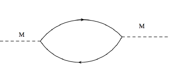
Figure 1: Nematic correlator: the full lines represent the composite fermion propagator, and the broken lines represent the nematic order parameters.

The propagator of the nematic order parameters in the Fermi liquid state is (here $\mathcal{T}$ denotes time ordering and $i,j=1,2$)

$$i\langle\mathcal{T}M_{i}M_{j}\rangle_{0}(\bm{p},\omega)\equiv\mathcal{L}^{-1}_{ij}(\bm{p},\omega)$$ (17)

The diagonal component $\mathcal{L}_{11}$ (represented diagrammatically in Fig.1) has the explicit form

$$\mathcal{L}_{11}(\bm{p},\Omega)=-i\int_{\bm{k},\omega}~{}g(\bm{k+p},\Omega+\omega)g(\bm{k},\omega)\left(\frac{k_{x}^{2}-k_{y}^{2}}{2m}\right)^{2}$$

$$=\frac{k_{F}^{4}}{4\pi m}-\cos^{2}(2\theta_{p})\frac{k_{F}^{3}}{2\pi}\left(\frac{i\Omega}{p}\right)+o(\Omega/p),$$

$$=\frac{V(0)}{4\pi l_{0}^{4}}-\cos^{2}(2\theta_{p})\frac{1}{2\pi l_{0}^{3}}\left(\frac{i\Omega}{p}\right)+o(\Omega/p)$$ (18)

where

$$g(\bm{k},\omega)=\frac{1}{\omega-\frac{\bm{k}^{2}-k_{F}^{2}}{2m}+i\eta\;\textrm{sign}(\omega)}$$ (19)

is the time-ordered free composite fermion propagator. In the same way, we can calculate the other components of $\mathcal{L}_{ij}(\bm{p},\omega)$ and replace $k_{F},m$ in terms of $l_{0},V(0)$,

$$\mathcal{L}_{12}(\bm{p},\Omega)= \cos(2\theta_{p})\sin(2\theta_{p})\frac{1}{2\pi l_{0}^{3}}\left(\frac{i\Omega}{p}\right),$$

$$\mathcal{L}_{22}(\bm{p},\Omega)= \frac{V(0)}{4\pi l_{0}^{4}}-\sin^{2}(2\theta_{p})\frac{1}{2\pi l_{0}^{3}}\left(\frac{i\Omega}{p}\right),$$ (20)

which agree with the results of OKF.Oganesyan et al. (2001)

Now we can include the gauge fluctuations. This is included through the loop expansion in the gauge fields, and we calculate only the one-loop corrections. In Appendix F and Appendix G we show that these corrections are subleading to the leading term, and thus do not change the dynamic scaling behavior of the critical theory of the nematic-isotropic phase transition.

IV Parity-odd Components of the nematic fluctuations: the Hall viscosity

In our earlier work,You and Fradkin (2013); You et al. (2014) we investigated the isotropic-nematic phase transition in FQH states and Chern insulators. We concluded that the theory describing the phase transition to the anisotropic state in such chiral topological phases always contains a Berry phase term for the nematic order parameters, which is odd under time reversal and parity. In the nematic FQH states the coefficient of the Berry phase term is related (but not equal to) with a dissipationless Hall viscosity.You et al. (2014); Cho et al. (2014) In Ref.[You et al., 2014] we concluded that the nematic fluctuation, regarded as a dynamical metric, only couples with the stress tensor of the composite fermion while the background metric also appears in the covariant derivative as the spin connection of the composite particle. Accordingly, the Berry phase of the nematic order parameter is the odd Hall viscosity of the mean-field state of the composite fermion theory, not of the electron fluid. Hence, in the incompressible FQH states, the Berry phase term is equivalent to the Hall viscosity of the composite fermion filling up integer number of the effective Landau levels.Cho et al. (2014); You et al. (2014)

For the compressible half-filled Landau levels, the mean field state of the composite fermion without the gauge fluctuation is a CFL with well-defined Fermi surface. Furthermore, the state is time-reversal even so we do not expect any Berry phase term for the nematic order parameters to emerge. However, once we include the dynamics of the gauge fluctuation $\delta a_{\mu}$ and go beyond the mean-field theory, the time-reversal symmetry is explicitly broken due to the Chern-Simons term for $\delta a_{\mu}$ and thus the Hall viscosity is expected to arise from the fluctuations. This is to be expected since, for the same reasons, the Hall conductivity of the CFL in the HLR theory also comes from gauge fluctuations.

To study the contribution from the gauge fluctuation to the Berry phase term, we formally integrate out the fermions at one-loop order, and rewrite the theory in terms of the fluctuating gauge field $\delta a_{\mu}$ and the nematic order parameter. Throughout this section we use the polarization functions of the compressible fermions $\Pi_{\mu\nu}$, $\Pi_{0}$ and $\Pi_{2}$, defined in Eqs.(89), (90) and (91), respectively, given explicitly in Appendix C. We first consider the linear coupling between the nematic field and the gauge field at the mean field level,

$$\mathcal{S}_{a,M}=-\int_{\bm{q},\omega}~{}\frac{1}{2}M_{i}(\bm{q},\omega)T_{i\nu}(\bm{q},\omega)\delta a_{\nu}(\bm{-q},-\omega),$$ (21)

where $T_{i\nu}(\bm{q},\omega)$ is the $2\times 3$ matrix (with $i=1,2$ and $\nu=t,x,y$)

$$T_{i\nu}(\bm{q},\omega)=\frac{m}{2\pi}\Pi_{2}(\bm{q},\omega)\begin{pmatrix}q_{x}^{2}-q_{y}^{2}&q_{x}\omega&-q_{y}\omega\\ -2q_{x}q_{y}&-\omega q_{y}&-q_{x}\omega\end{pmatrix}.$$ (22)

is the effective vertex. This coupling can be regarded as the symmetric part of the Wen-Zee-like term which we will discuss later.

Beyond this, there is another term involving the fluctuating nematic order parameter and Chern-Simons gauge fields.

$$\mathcal{S}_{a,M,a}=-\frac{1}{2}\int_{\bm{q},\omega}\delta a_{\mu}(\bm{q},\omega)\mathcal{V}_{\mu\nu}(\bm{q},\omega)\delta a_{\nu}(\bm{-q},-\omega),$$ (23)

where

$$\mathcal{V}_{\mu\nu}(\bm{q},\omega)=\frac{\Pi_{0}(\bm{q},\omega)}{2\pi}\begin{pmatrix}\frac{M_{1}}{2}(q_{x}^{2}-q_{y}^{2})&(M_{1}q_{x}+M_{2}q_{y})\omega&(-M_{2}q_{y}+M_{2}q_{x})\omega\\ (M_{1}q_{x}+M_{2}q_{y})\omega&M_{1}\omega^{2}&M_{2}\omega^{2}\\ (-M_{2}q_{y}+M_{2}q_{x})\omega&M_{2}\omega^{2}&-M_{1}\omega^{2}\end{pmatrix}.$$ (24)

This term is the coupling to the dynamical metric or nematic order parameter of the Maxwell term for the fluctuating gauge field $\delta a_{\mu}$. As the nematic order parameter can be considered as a dynamical metric that modifies the local metric of the composite fermion, the gauge boson coupled to the fermion is also modified accordingly by the nematic order parameter.

Together with the original isotropic HLR result for the action of the fluctuating Chern-Simons field $\delta a_{\mu}$

$$\mathcal{S}_{a}=-\frac{1}{2}\int_{\bm{q},\omega}\delta a_{\mu}(\bm{q},\omega)\Pi_{\mu\nu}(\bm{q},\omega)\delta a_{\nu}(-\bm{q},-\omega),$$ (25)

we can obtain the Berry phase term of the nematic order parameter by integrating out the fluctuating gauge fields and performing the loop expansions. In the following, we fix the gauge $a_{0}=0$ to facilitate the calculation.

The effective action $\mathcal{S}=\mathcal{S}_{a}+\mathcal{S}_{a,M,a}$ of the gauge field $\delta a_{\mu}$, defined by Eq.(7) and Eq.(8), coupled with the nematic order parameter $\bm{M}$, is

$$\mathcal{S}=-\frac{1}{2}\int_{\bm{q},\omega,\bm{k},\Omega}\delta a_{i}(\bm{q},\omega)\Big{[}\Pi_{ij}+(t^{1}_{ij}\omega^{2}\Pi_{0})M_{1}+(t^{2}_{ij}\omega^{2}\Pi_{0})M_{2}\Big{]}\delta a_{j}(\bm{-q},-\omega)$$ (26)

where the $2\times 2$ matrices $t^{1}_{ij}$ and $t^{2}_{ij}$ denote the Pauli matrices $\sigma_{3}$ and $\sigma_{1}$, respectively, and $\bm{M}$ are the nematic fields. By integrating out the fluctuations of the gauge fields, and performing the loop expansion, we obtain leading corrections to the (time-ordered) correlators of the nematic order parameter $\bm{M}$ (shown in the Feynman diagram of Fig. 2)

$$\langle\delta M_{i}\delta M_{j}\rangle(\Omega,\bm{p})=i\int_{\bm{q},\omega}\textrm{tr}\left[\Pi_{ij}^{-1}(\omega,\bm{q})\;\omega^{2}\Pi_{0}t^{i}\;\Pi_{ij}^{-1}(\omega+\Omega,\bm{q+p})\;\omega^{2}\Pi_{0}t^{j}\right]$$

$$=i\frac{\Omega}{2}\epsilon^{ij}~{}\int_{\bm{q},\omega}~{}\frac{\Pi_{2}\bm{q}^{2}}{\Pi_{2}\bm{q}^{2}+\bm{q}^{2}/4}\frac{\sqrt{{\bar{\rho}}}}{\Pi_{2}\bm{q}^{2}+\bm{q}^{2}/4}+....$$ (27)

where we have approximate the form of the polarization tensor $\Pi_{ij}(\omega,\bm{q})$ valid for low frequency and momentum with $\omega\ll|\bm{q}|v_{F}$ (see Appendix B).

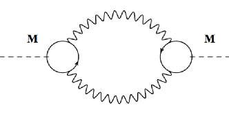
Figure 2: Berry phase term. Here the bubble is the fermion loop corrected by the fluctuating gauge field.

Hence, the anti-symmetric (and hence off-diagonal) part of the nematic correlator $\mathcal{L}^{-1}_{ij}$ gives a Berry phase type term in the effective action for the nematic fields

$$\mathcal{S}^{M}_{ij}=\int_{\bm{p},\Omega}\chi\epsilon^{ij}(i\Omega)M_{i}(\bm{p},\Omega)M_{j}(-\bm{p},-\Omega),$$ (28)

where

$$\chi=\frac{2}{3\pi}\bar{\Lambda}m=\frac{2}{3\pi l_{0}^{2}}$$ (29)

with $\bar{\Lambda}$ the high-frequency cutoff of the CFL and $m$ is the effective mass of the composite fermions. Using the HLR resultsHalperin et al. (1993) (see Appendix B), since the UV cutoff ${\bar{\Lambda}}=E_{F}^{\rm CFL}$ (the Fermi energy of the CFL), and the value of the effective mass $m$ (which in the HLR theory is argued to depend only on the scale of the Coulomb interaction) one finds that $m{\bar{\Lambda}}=\ell_{0}^{-2}$, and hence that the Hall viscosity seemingly depends only on the particle density. This value of the Berry phase $\chi$ is one of our main results in this paper. It plays a key role in the effective dynamics of the nematic order parameters. However, we should caution that, contrary to the case of the FQH states, this value of the Hall viscosity is not protected in the CFL, and should be regarded as an estimate.

Our result indicates that the gauge field fluctuations generate a Berry phase term which will in turn contribute to the Hall viscosity of the compressible half-filled Landau levels. The way in which the Berry phase term is generated in this case is different from that of the incompressible FQH states. In the incompressible FQH states, the Berry phase of nematic order parameters is already present at the mean field level of the composite fermion which forms an integer quantum Hall state, due to the explicitly broke the time-reversal symmetry of the composite fermions in the effective Landau level.Cho et al. (2014); You et al. (2014) Furthermore, the Chern-Simons gauge fields in the FQH state are gapped and do not affect the value of the Berry phase term in the low energy regime. In contrast, for compressible half-filled Landau levels, the mean field state is a Fermi liquid alone which seemingly respects time-reversal symmetry, which is broken by the Chern-Simons term for the gauge fields. Their fluctuations can affect the low-energy dynamics of the nematic order parameters and induce the non-zero Berry phase term for the nematic order parameters. In particular, while in the incompressible FQH states the coefficient of the Berry phase term has a universal relation with the composite fermion density, in the case of the compressible state this “Hall viscosity” is non-universal as it depends explicitly on the UV energy cutoff $\bar{\Lambda}$ of the compressible composite Fermi fluid.

V Ward Identities

We now present another way to compute and check the Berry phase term, Eq.(28). Here we will use the Ward identity between the current operators $\bm{J}$ and the stress tensor $T_{ij}$ (and the linear momentum density $T_{0j}$). We start with the explicit expressions for these operators in the CFL,

$$J_{i}=\frac{1}{2m}[\Psi^{\dagger}(\bm{r},t)(\partial_{i}+i\delta a_{i})\Psi-((\partial_{i}+i\delta a_{i})\Psi^{\dagger})\Psi(\bm{r},t)],$$

$$T_{ij}=\frac{1}{2m}\Psi^{\dagger}(\bm{r},t)(\partial_{i}+i\delta a_{i})(\partial_{j}+i\delta a_{j})\Psi(\bm{r},t),$$

$$T_{0j}=mJ_{j}.$$ (30)

which are manifestly gauge invariant.

The conservation law of the energy-momentum tensor (i.e. local conservation of energy and momentum), in the presence of the Chern-Simons gauge field fluctuations, implies that

$$\partial_{\mu}T_{\mu i}=\delta b~{}\epsilon^{ij}J_{j},$$ (31)

where $\delta b=\varepsilon_{ij}\partial_{i}\delta a_{j}$ is the fluctuating flux of the gauge field $\delta a_{\mu}$. Upon expanding out in components the expression of Eq.(31), we have

$$\partial_{0}mJ_{x}+\partial_{x}T_{xx}+\partial_{y}T_{yx}=\delta bJ_{y},$$

$$\partial_{0}mJ_{y}+\partial_{x}T_{xy}+\partial_{y}T_{yy}=-\delta bJ_{x}.$$ (32)

In what follows we will use the notation $T_{1}=T_{xx}-T_{yy}$, and $T_{2}=T_{xy}+T_{yx}$. Focusing only on the anti-symmetric response, we find the following relation between the correlation functions of current, stress tensor and density operators,

$$\partial^{2}_{t_{1}}m^{2}\langle J_{x}(\bm{r}_{1},t_{1})J_{y}(\bm{r}_{2},t_{2})\rangle+\partial^{2}_{\bm{r}_{1}}\langle T_{1}(\bm{r}_{1},t_{1})T_{2}(\bm{r}_{2},t_{2})\rangle$$

$$=4\langle\rho(\bm{r}_{1},t_{1})J_{x}(\bm{r}_{1},t_{1})\rho(\bm{r}_{2},t_{2})J_{y}(\bm{r}_{2},t_{2})\rangle.$$ (33)

Hence the Berry phase term, i.e. the Hall viscosity determined by the parity-odd correlation function of the stress tensor,Read and Rezayi (2011); Bradlyn et al. (2012); Gromov and Abanov (2014); Cho et al. (2014); Gromov et al. (2015); You et al. (2014); Bradlyn and Read (2015) is related with the correlation function of the composite operators of densities and currents (shown on on the right side of Eq.(33)). In momentum and frequency space (and in the low frequency limit, $\Omega\to 0$) this results takes the form

$$\bm{p}^{2}\langle T_{1}T_{2}\rangle(\bm{p},\Omega) =\int_{\bm{q},\omega}~{}[4\langle\rho\rho\rangle(\bm{p-q},\omega+\Omega)\langle J_{x}J_{y}\rangle(\bm{q},\omega)$$

$$+4\langle\rho J_{y}\rangle(\bm{p-q},\omega+\Omega)\langle J_{x}\rho\rangle(\bm{q},\omega)]$$ (34)

The density and current correlators, $\langle\rho\rho\rangle$ and $\langle J_{x}J_{y}\rangle$, are given by the polarization tensor of the external electromagnetic gauge field beyond the mean field level which include the fluctuations of the Chern-Simons gauge field.

$$\langle\rho\rho\rangle(\omega,\bm{q})=\frac{1}{4(2\pi)}\frac{\Pi_{0}q^{2}}{D(\omega,\bm{q})}$$

$$\langle J_{x}J_{y}\rangle(\omega,\bm{q})=\frac{i\omega}{2(2\pi)},$$

$$\langle\rho J_{y}\rangle(\omega,\bm{q})=-\frac{1}{4(2\pi)}\frac{\Pi_{0}q_{y}\omega}{D(\omega,\bm{q})}-\frac{iq_{x}}{2(2\pi)},$$

$$\langle J_{x}\rho\rangle(\omega,\bm{q})=-\frac{1}{4(2\pi)}\frac{\Pi_{0}q_{x}\omega}{D(\omega,\bm{q})}-\frac{iq_{y}}{2(2\pi)},$$

$$D(\omega,\bm{q})=\frac{1}{2\pi}\Big{(}\Pi_{0}^{2}\omega^{2}-\frac{1}{4}-\Pi_{0}q^{2}(\Pi_{2}+\frac{V(q)}{16\pi^{2}})\Big{)}.$$ (35)

Using these relations we obtain a result consistent with the previous approach,

$$\langle T_{1}T_{2}\rangle(\Omega,\bm{p})=\partial_{p^{2}}4\langle\rho J_{x}\rho J_{y}\rangle(\Omega,\bm{p})$$

$$=i\Omega\frac{2}{3\pi}m\bar{\Lambda}=i\Omega\frac{2}{3\pi l_{0}^{2}}$$ (36)

VI Effective Dynamics and Susceptibility of the Nematic Order

With the results of the calculation of the Berry phase term and Landau damping terms for the nematic order parameters at hand, we can proceed to derive the expression for the nematic correlators including both contributions. The effective theory for the nematic order parameter field $\bm{M}$ close to the nematic transition is

$$\mathcal{S}[\bm{M}]= \int_{\bm{p},\Omega}M_{i}(\bm{p},\Omega)\mathcal{L}_{ij}M_{j}(-\bm{p},-\Omega)-\int d^{3}x\lambda\bm{M}^{4}$$ (37)

in which the correlator $\mathcal{L}_{ij}(\bm{p},\omega)$ is given by the sum of the two contributions, which yields the result

$$\mathcal{L}_{ij}=\begin{pmatrix}-\frac{\kappa}{2F_{2}}p^{2}-\delta-\cos^{2}(2\theta_{p})\frac{1}{2\pi l_{0}^{3}}(\frac{i\Omega}{p})&i\Omega(\frac{2}{3\pi l_{0}^{2}})+\sin(2\theta_{p})\cos(2\theta_{p})\frac{1}{2\pi l_{0}^{3}}(\frac{i\Omega}{p})\\ -i\Omega(\frac{2}{3\pi l_{0}^{2}})+\sin(2\theta_{p})\cos(2\theta_{p})\frac{1}{2\pi l_{0}^{3}}(\frac{i\Omega}{p})&-\frac{\kappa}{2F_{2}}p^{2}-\delta-\sin^{2}(2\theta_{p})\frac{1}{2\pi l_{0}^{3}}(\frac{i\Omega}{p})\end{pmatrix},$$ (38)

where $\delta$ is the distance to the Pomeranchuk instability of Eq.(12). As in the case of the nematic Fermi fluid, $\mathcal{L}_{ij}(\bm{p},\omega)$ is nothing but the inverse susceptibility of the nematic order parameters, and zeros of the determinant of $\mathcal{L}_{ij}(\bm{p},\omega)$ yield the dispersion relation of the nematic collective modes of the CFL. Clearly the nematic susceptibility is finite for $\delta>0$ and diverges as $\delta\to 0$, as expected at a continuous quantum phase transition.

Except for the Hall viscosity term, which originates from the gauge fluctuations which explicitly break the time-reversal symmetry, Eq.(38) is almost the same as the result for the nematic correlator of OKF.Oganesyan et al. (2001) The Berry phase term, which makes the effective theory time-reversal odd, mixes the transverse and longitudinal modes of the nematic order parameters. However, if we focus only on the parameter regime where $q\ll k_{F}$ and $\omega\ll v_{F}q$, then the off-diagonal terms are sub-dominant and can be ignored. Hence the overdamped critical mode is not affected by the gauge fluctuations. This leads to the conclusion that the criticality of the isotropic-anisotropic phase transition of half-filled LL still exhibits $z=3$ critical dynamical exponent.

VI.1 Nematic Susceptibility

From the effective theory Eq.(38), we can read-off the dynamic nematic susceptibility $\chi^{M}$, i.e. the nematic propagator. Inside the isotropic phase, $\delta>0$, the susceptibility is given by

$$\chi^{M}_{ij}=\mathcal{L}^{-1}_{ij}=\frac{1}{C(\Omega,{\bm{p}})}\begin{pmatrix}-\frac{\kappa}{2F_{2}}p^{2}-\delta-\sin^{2}(2\theta_{p})\frac{1}{2\pi l_{0}^{3}}(\frac{i\Omega}{p})&i\Omega(\frac{2}{3\pi l_{0}^{2}})-\sin(2\theta_{p})\cos(2\theta_{p})\frac{1}{2\pi l_{0}^{3}}(\frac{i\Omega}{p})\\ -i\Omega(\frac{2}{3\pi l_{0}^{2}})-\sin(2\theta_{p})\cos(2\theta_{p})\frac{1}{2\pi l_{0}^{3}}(\frac{i\Omega}{p})&-\frac{\kappa}{2F_{2}}p^{2}-\delta-\cos^{2}(2\theta_{p})\frac{1}{2\pi l_{0}^{3}}(\frac{i\Omega}{p})\end{pmatrix}$$ (39)

where

$$C(\Omega,\bm{p})=(\frac{\kappa}{2F_{2}}p^{2}+\delta)^{2}+(\frac{\kappa}{2F_{2}}p^{2}+\delta)\frac{1}{2\pi l_{0}^{3}}(\frac{i\Omega}{p})-\Omega^{2}(\frac{2}{3\pi l_{0}^{2}})^{2}\approx\delta^{2}+\delta\frac{1}{2\pi l_{0}^{3}}\frac{i\Omega}{p}.$$ (40)

The nematic susceptibility is finite in the isotropic phase where $\frac{1}{2\pi l_{0}^{3}}\frac{i\Omega}{p}\ll 1$. As we approach the quantum critical point, $\delta\rightarrow 0$, the nematic susceptibility diverges, as expected. In the nematic phase, we assume the the nematic order is in the $M_{1}$ direction ($M_{1}=\sqrt{\frac{|\delta|}{2\lambda}}$). The nematic susceptibility in the symmetry broken phase can be obtained,

$$\chi^{M}_{ij}(\Omega,{\bm{p}})=\frac{1}{C^{\prime}(\Omega,\bm{p})}\begin{pmatrix}-\frac{\kappa}{2F_{2}}p^{2}-|\delta|-\sin^{2}(2\theta_{p})\frac{1}{2\pi l_{0}^{3}}(\frac{i\Omega}{p})&i\Omega(\frac{2}{3\pi l_{0}^{2}})-i\sin(2\theta_{p})\cos(2\theta_{p})\frac{1}{2\pi l_{0}^{3}}(\frac{i\Omega}{p})\\ -i\Omega(\frac{2}{3\pi l_{0}^{2}})-i\sin(2\theta_{p})\cos(2\theta_{p})\frac{1}{2\pi l_{0}^{3}}(\frac{i\Omega}{p})&-\frac{\kappa}{2F_{2}}p^{2}-\cos^{2}(2\theta_{p})\frac{1}{2\pi l_{0}^{3}}(\frac{i\Omega}{p})\end{pmatrix}$$ (41)

where

$$C^{\prime}(\Omega,\bm{p})\approx(\frac{\kappa}{2F_{2}}p^{2}+\frac{1}{2\pi l_{0}^{3}}\frac{i\Omega}{p}\sin^{2}(2\theta_{p}))|\delta|,$$ (42)

VI.2 Mode mixing in the Nematic phase and at quantum criticality

In the theory of the nematic transition in a Fermi liquid of OFK, when approaching the criticality, $\delta\rightarrow 0$, the difference in the dynamics of the two polarizations becomes more noticeable. At criticality there is an underdamped longitudinal mode $\omega_{T}\sim q^{2}$ and an overdamped transverse mode $\omega_{L}\sim iq^{3}$. In the nematic phase this mode becomes the (overdamped) Goldstone mode. In our nematic criticality in the half-filled LL, due to the existence of the Berry phase term, the transverse and longitudinal modes are mixed, leading to the following modified dispersions for these collective modes

$$\omega_{1} \sim\frac{\sqrt{\kappa V(0)}l_{0}}{\sqrt{2F_{2}\pi}}q^{2}+i\frac{l_{0}V(0)}{2}q^{3},$$

$$\omega_{2} \sim i\frac{\kappa}{2F_{2}(\pi/l_{0}^{2})^{3/2}}q^{3}$$ (43)

Thus, the transverse mode, $\omega_{2}$, remains overdamped (as in the OKF theory). In contrast, the longitudinal mode, $\omega_{1}$, is now underdamped (with $z=2$) only in the deep asymptotic long-wavelength regime $q\to 0$, crossing over to an overdamped regime at larger values of $q$. This crossover can happen at long wavelengths if the range of the quadrupolar interaction is small.

VI.3 Electromagnetic Response and Spectral Peak

In the nematic phase, the electromagnetic response (and the conductivity tensor) can be obtained after integrating out the gauge fluctuations. The calculation details of the electromagnetic response is presented in Appendix B. Here we propose a possible experimental test of the nematicity by measuring the spectrum of the conductivity $\sigma_{xx}$. To this end, let us assume that we are in the deep nematic phase with a nonzero nematic order, say in the $M_{1}$ component. The conductivity $\sigma_{xx}$ as a function of momentum is,

$$\sigma_{xx} =\frac{i}{\omega}\langle J_{x}J_{x}\rangle=-\omega\Pi_{0}(\bm{q},\omega)\frac{(1+M_{1})}{4D^{\prime}(\bm{q},\omega)},$$

$$D^{\prime}(\bm{q},\omega) =\Pi_{0}(\bm{q},\omega)\left(\Pi_{2}(\bm{q},\omega)-\frac{V(\bm{q})}{16\pi^{2}}\right)({\bm{q}}^{2}+M_{1}(q_{x}^{2}-q_{y}^{2}))$$

$$-\frac{1}{4}+\Pi^{2}_{0}(\bm{q},\omega)\omega^{2}$$ (44)

In the limit of $\omega/q\ll 1$, the conductivity is approximately given by

$$\sigma_{xx}\sim\frac{\omega(1+M_{1})/V(0)}{(1+M_{1}\cos(2\theta_{q}))i\frac{\omega}{qV(0)l_{0}}+\frac{\omega^{2}}{V(0)^{2}q^{2}}-q^{2}/4}$$ (45)

Deep nematic phase where $M_{1}\sim O(1)$, the damping term on the denominator will nearly vanish at $\theta_{q}=\pi/2$. Thus, by measuring $\sigma_{xx}$ as a function of the angle $\theta_{q}$ of the direction of propagation measured form the nematic axis, one will find a resonance, i.e. a peak in the spectrum, at $\theta_{q}=\pi/2$.

VII The Wen-Zee term in the CFL

From the Hall viscosity term, we expect that there may be the Wen-Zee type terms for the dynamical metric associated with the nematic order parameters.You et al. (2014); Maciejko et al. (2013) The Wen-Zee like term consists of two parts: a parity-even term linear in nematic order parameter and in the gauge field, and a second term that is parity-odd, and is quadratic in nematic order parameter and linear in gauge field. At the mean field level of the CFL, which is parity-even except for the Chern-Simons term, the composite fermions on the Fermi surface generate only the parity-even part of the Wen-Zee term. However, upon the inclusion of the gauge field fluctuations, which are parity-odd, we will find the parity-odd part of the Wen-Zee term, as well as a modification of the parity-even part.

We start by calculating the first part of the Wen-Zee term given by a Feynman diagram that has one gauge leg and one nematic leg shown below in Fig. 3. The coupling between gauge-invariant current, generated by the probe electromagnetic gauge fields $A_{\mu}$, and nematic order parameter $\bm{M}$ is given by

$$(-i)\frac{\delta\mathcal{S}}{\delta M_{l}\delta A_{k}}(\bm{p},\Omega)\equiv\langle M_{l}J_{k}\rangle({\bm{p}},\Omega)$$

$$= i\int_{\bm{q},\omega}~{}\textrm{tr}\Big{[}\Pi_{ij}^{-1}(\omega,\bm{q})\omega^{2}\Pi_{0}t_{l}T^{-1}_{mi}(\omega+\Omega,\bm{q+p})\omega^{2}\Pi_{0}Q_{k}\Big{]},$$

$$= \frac{1}{6\pi\sqrt{3}}(\frac{\bar{\Lambda}m}{{\bar{\rho}}})^{1/3}\begin{pmatrix}p_{x}\Omega&p_{y}\Omega\\ -\Omega p_{y}&p_{x}\Omega\end{pmatrix}_{lk},$$ (46)

Figure 3: Leading parity-even contribution to the Wen-Zee term. The wavy lines are gauge field propagators and the broken line is a nematic propagator. The blobs are composite fermion loops.

where, as before, $t_{1}=\sigma_{3}$ and $t_{2}=\sigma_{1}$, and where we used the notation $Q_{x}=I$ and $Q_{y}=-i\sigma_{2}$, and $T^{-1}_{mi}$ is given by

$$T^{-1}_{mi}=\langle a_{m}M_{i}\rangle=\frac{1}{\Pi_{2}mq^{2}\omega^{2}}\begin{pmatrix}q_{x}\omega&q_{y}\omega\\ -\omega q_{y}&q_{x}\omega\end{pmatrix}$$ (47)

where we used the temporal gauge, $a_{0}=0$. This is the parity-even linear coupling between the nematic order parameter and the probe electromagnetic gauge field.

To calculate the parity-odd contributions to the Wen-Zee term, we calculate a Feynman diagram with one external probe gauge field leg and two nematic order parameter legs. Once again we choose the gauge $a_{0}=0$, and find the result

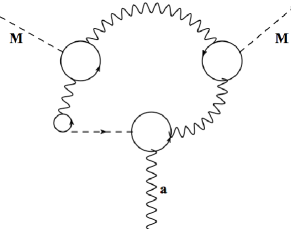
Figure 4: Parity-odd contribution to the Wen-Zee term at cubic level. The wavy lines are gauge field propagators and the broken line is a nematic propagator.

$$(-i)\frac{\delta\mathcal{S}}{\delta M_{h}\delta M_{l}\delta A_{k}} (\Omega_{1},\Omega_{2};\bm{p}_{1},\bm{p}_{2})\equiv\langle M_{h}M_{l}J_{k}\rangle(\Omega_{1},\Omega_{2};\bm{p}_{1},\bm{p}_{2})$$

$$=\int_{\bm{q},\omega}~{}\textrm{tr}\Big{[}\Pi_{ij}^{-1}(\omega,\bm{q})\omega^{2}\Pi_{0}\sigma_{h}\Pi_{ij}^{-1}(\omega+\Omega_{1},\bm{q+p_{1}})\omega^{2}\Pi_{0}\sigma_{l}T^{-1}_{mi}(\omega+\Omega_{1}+\Omega_{2},\bm{q+p_{1}+p_{2}})\omega^{2}\Pi_{0}Q_{k}\Big{]}$$

$$=\frac{1}{6\pi\sqrt{3}}[(\frac{\bar{\Lambda}m}{{\bar{\rho}}})^{1/3}+\frac{\bar{\Lambda}m}{{\bar{\rho}}}]\epsilon^{hl}\epsilon^{\nu\mu k}p_{1}^{\nu}(p_{1}^{\mu}+p_{2}^{\mu})$$ (48)

which is manifestly odd under parity and time reversal symmetries.

By combining the two contributions, we finally find a Wen-Zee term of the form

$$\mathcal{L}_{WZ}=\frac{1}{6\pi\sqrt{3}}\Big{[}\left(\frac{\bar{\Lambda}m}{{\bar{\rho}}}\right)^{1/3}+\frac{\bar{\Lambda}m}{{\bar{\rho}}}\Big{]}\epsilon^{\mu\nu\rho}\omega_{\mu}\partial_{\nu}A_{\rho}$$ (49)

where $\bar{\Lambda}$ is the frequency UV cutoff of the CFL. Further reduce the expression by taking $\bar{\Lambda}m=l_{0}^{-2}$, we have,

$$\mathcal{L}_{WZ}=\frac{2}{3\pi\sqrt{3}}\epsilon^{\mu\nu\rho}\omega_{\mu}\partial_{\nu}A_{\rho}$$ (50)

Here we have denoted by $\omega_{\mu}$ the spin connection associated with the nematic fields,You et al. (2014)

$$\omega_{0}=\epsilon^{ij}M_{i}\partial_{0}M_{j}$$ (51)

$$\omega_{x}=\epsilon^{ij}M_{i}\partial_{x}M_{j}-(\partial_{x}M_{2}-\partial_{y}M_{1})$$

$$\omega_{y}=\epsilon^{ij}M_{i}\partial_{y}M_{j}+(\partial_{x}M_{1}+\partial_{y}M_{2})$$

Similar to what we did for the calculation of the Berry phase term using a Ward Identity, the Wen-Zee term can also be derived from the Ward Identity, and the result is consistent with the diagrammatic calculation present here. The details of the calculation of Wen-Zee term from Ward Identity is presented in the Appendix E.

We should stress that the connection between the Hall viscosity (given by the Berry phase term) and the Wen-Zee term in the CFL is not as straightforward as in the incompressible FQH states. In the incompressible states, the universal coefficients $s$ of the Wen-Zee term is directly related to the Hall viscosity $\eta_{H}$, i.e., $\eta_{H}=\frac{s{\bar{\rho}}}{2}$.Read (2009); Read and Rezayi (2011); Cho et al. (2014); Gromov et al. (2015) However, in the compressible CFL state, the coefficients of the Wen-Zee term and the Hall viscosity do not have such relation because of the non-local nature of such responses in a compressible state. The coefficients appearing in the expressions are seemingly numeric constants, but it is important to remember that the coefficients are in fact the functions of the ratio $s=\frac{|\Omega|}{v_{F}|\bm{q}|}$ (not to be confused with the coefficient of the Wen-Zee term!), and are in general non-local in space and time. Instead, in the incompressible states where we can perform the well-defined gradient expansions due to the energy gap to all the excitations. Hence we find that in the CFL, the coefficients of the (seemingly local) Wen-Zee term and Hall viscosities are not universally related to each other.

VII.1 Nematic-Electric field correlator

The Wen-Zee-type term Eq.(50), which couples the nematic field and the electromagnetic field, implies that the change in the nematic field will induce the electron quadrupole moment. Thus, one can measure the nematic susceptibility with respect to the external electric field $\chi_{M,E}=\frac{\partial T_{i}}{\partial E_{j}}$ as a function of momentum,

$$\chi_{M,E}=\frac{\delta^{2}\mathcal{S}}{\delta M_{i}\delta E_{j}}(\bm{q})=\frac{\partial T_{i}}{\partial E_{j}},$$

$$=\frac{2}{3\pi\sqrt{3}}\begin{pmatrix}-q_{x}&q_{y}\\ -q_{y}&-q_{x}\end{pmatrix}.$$ (52)

This susceptibility indicates that the energy-momentum current will be induced in the presence of the spatially-modulating electric field.

VIII General relation between the Hall viscosity and the hydrodynamic gauge theory in half-filled Landau levels

We have shown that, unlike the case of the incompressible FQH states, in the CFL the gauge field fluctuations contribute to the Hall viscosity of the half-filled Landau level. In order to prove that the corrections to the Hall viscosity come from the fluctuation of the Chern Simons gauge fields, we start from CFL and dualize the CFL into a hydrodynamic gauge theory.

If we couple our CFL to a smooth deformation of the background geometry (instead of to the nematic order parameter), we find that the composite fermions at the mean field level receive an orbital spin from the flux attachment procedure.Cho et al. (2014) Beyond this, if we include the gauge field fluctuation, the viscoelastic response of the CFL is related with the parity-odd electromagnetic response of the hydrodynamic gauge theory.Hoyos and Son (2012); Read and Rezayi (2011) Since the original CFL is coupled to the fluctuating Chern-Simons gauge boson, the time-reversal odd electromagnetic response of the hydrodynamic gauge theory is always non-zero. Consequently, the CFL contains an additional contribution to the Hall viscosity arising from the fluctuating gauge field.

To see this, we start from the Chern-Simons theory of CFL where we attach two flux quanta of the Chern-Simons gauge field to the electrons to turn them into the composite fermions,

$$\mathcal{S}=\int dr^{2}dt~{}\Psi^{\dagger}\Big{(}\bm{r},t)(iD_{t}+\frac{1}{2m}{\bm{D}}^{2}+\frac{g_{ij}}{2m}D_{i}D_{j}\Big{)}\Psi(\bm{r},t)$$

$$-\frac{1}{2}\int dr^{\prime 2}dr^{2}dt~{}V(\bm{r-r^{\prime}})\rho({r})\rho({r^{\prime}})$$

$$+\int dr^{2}dt~{}\frac{1}{8\pi}\epsilon^{\mu\nu\rho}a_{\mu}\partial_{\nu}a_{\rho}$$ (53)

where $D_{\mu}=\partial_{\mu}+i(A_{\mu}+a_{\mu}+\omega_{\mu})$ is the covariant derivative. Here, $\omega_{\mu}$ is the spin connection of the background metric $g_{ij}$, which is related to the local frame fields by $g_{ij}=(e^{a}_{j}+\delta^{a}_{j})(e^{a}_{i}+\delta^{a}_{i})$. We only keep the leading orders in $e^{a}_{i}$ so that the distorted spatial metric is defined as,

$$\delta g_{ij}=\begin{pmatrix}e_{1}^{1}&e_{1}^{2}\\ e_{2}^{1}&e_{2}^{2}\end{pmatrix}.$$ (54)

The composite fermion has orbital spin $s=1$Cho et al. (2014) so the covariant derivative of the composite fermion contains the spin connection with coefficient $1$ dictated by the orbital spin $s=1$. At the mean field level, the Chern-Simons flux cancels the external magnetic fields so we only need to consider the gauge fluctuation $\delta a$.

We can now perform the functional bosonization procedure, following Refs.[Fradkin and Schaposnik, 1994; Le Guillou et al., 1997; Fradkin, 2013; Chan et al., 2013], of our theory and introduce the hydrodynamic gauge field $b_{\mu}$,Wen (1995)

$$\mathcal{S}=\int dr^{2}dt~{}\Psi^{\dagger}(\bm{r},t)(iD_{t}+\frac{1}{2m}D_{i}D_{i}+\frac{g_{ij}}{2m}D_{i}D_{j})\Psi(\bm{r},t)$$

$$-\frac{1}{32\pi^{2}}\int dr^{\prime 2}dr^{2}dt~{}V(\bm{r-r^{\prime}})\delta b(\bm{r})\delta b(\bm{r}^{\prime})$$

$$-\int dr^{2}dt~{}\frac{2}{4\pi}\epsilon^{\mu\nu\rho}b_{\mu}\partial_{\nu}b_{\rho}+\int dr^{2}dt~{}\frac{1}{2\pi}\epsilon^{\mu\nu\rho}\delta a_{\mu}\partial_{\nu}b_{\rho}$$ (55)

where $D_{\mu}=\partial_{\mu}+i(\delta a_{\mu}+\omega_{\mu})$ is the covariant derivative , and $\delta b(\bm{r})=\partial_{x}\delta a_{y}(\bm{r})-\partial_{y}\delta a_{x}(\bm{r})$ is the fluctuating magnetic flux of the gauge field $\delta a_{\mu}$.

Solving the saddle-point equation of $\delta a_{\mu}$, we find

$$\partial_{x}b_{0}-\partial_{0}b_{x}= E^{b}_{x}=J^{CF}_{y},$$

$$\partial_{y}b_{0}-\partial_{0}b_{y}= E^{b}_{y}=-J^{CF}_{x},$$

$$\partial_{x}E^{b}_{x}= T^{CF}_{12}=\Psi^{\dagger}\frac{D_{x}D_{y}}{2m}\Psi,$$

$$\partial_{y}E^{b}_{y}= -T^{CF}_{21}=-\Psi^{\dagger}\frac{D_{y}D_{x}}{2m}\Psi$$ (56)

Now we turn on a momentum current of the composite fermion $T^{CF}_{12}$ in the system. Different from the parity-even Fermi surface where the metric only couples with the momentum current, the composite fermions carry intrinsic orbital spin so the spin connection appears in the covariant derivative. Hence,

$$\frac{\delta\mathcal{S}}{\delta e_{1}^{2}}=T^{CF}_{12}+(\partial_{\mu}e^{1}_{1})J^{CF}_{\mu}.$$ (57)

The composite fermion current $T^{CF}_{12}$ is bound with the spatial derivative of electric field of $b_{\mu}$ as $\partial_{x}E^{b}_{x}$. Once we have a nonzero $\partial_{x}E^{b}_{x}$, a polarized charge density appears. If the hydrodynamic gauge theory of the gauge field $b_{\mu}$ contains a term like $\beta(\nabla\cdot E^{b})B^{b}$, the polarized charge density associated with the field $b_{\mu}$ acts as a magnetic moment which couples with magnetic flux of $b_{\mu}$. Thus, we have

$$\frac{\delta\mathcal{S}}{\delta(\partial_{x}b_{y})}=\beta\partial_{x}(\partial_{x}b_{0}-\partial_{0}b_{x})$$ (58)

By solving the equation of motion for the hydrodynamic gauge field,

$$\frac{\delta\mathcal{S}}{\delta(\partial_{x}b_{y})}=\partial_{0}\frac{\delta\mathcal{S}}{\delta\partial_{0}(\partial_{x}b_{y})}$$

$$\frac{\delta\mathcal{S}}{\delta\partial_{0}(\partial_{x}b_{y})}=\frac{\delta\mathcal{S}}{\delta\partial_{x}(\partial_{0}b_{y})}=\frac{\delta\mathcal{S}}{\delta T_{11}}=e_{1}^{1}$$ (59)

We finally have

$$\frac{\delta\mathcal{S}}{\delta(\partial_{x}b_{y})}=\partial_{0}e_{1}^{1}=\beta\partial_{x}(\partial_{x}b_{0}-\partial_{0}b_{x}).$$ (60)

Thus the Hall viscosity can be read off from

$$\frac{\delta\mathcal{S}}{\delta e_{1}^{2}}=\frac{1}{\beta}\partial_{0}e_{1}^{1}+(\partial_{\mu}e^{1}_{1})J^{CF}_{\mu}=(\rho+\frac{1}{\beta})\partial_{0}e_{1}^{1},$$ (61)

i.e., the Hall viscosity is $(\rho+\frac{1}{\beta})$ in which $\rho$ is due to the flux attachment,Cho et al. (2014) and $1/\beta$ is due to the parity-odd fluctuations of the hydrodynamic gauge field. The parity-odd viscosity has two contributions: one is the intrinsic orbital spin that the composite fermion carries, and the other is through the term $(\nabla\cdot E^{b})B^{b}$ of the hydrodynamic gauge field. Hence, if the dual hydrodynamic gauge theory has the parity-odd $\beta(\nabla\cdot E^{b})B^{b}$ term, we expect that there should be additional Hall viscosity from the gauge fluctuation. The theory of the $b_{\mu}$ field can be obtained by integrating out the composite fermion surface and gauge fluctuation of the gapless $a_{\mu}$. However, if the effective theory of $a_{\mu}$ is gapless and nonlocal, the coefficient $\beta$ for the term $(\nabla\cdot E^{b})B^{b}$ will be non-universal (and depend on the UV cutoff in a singular way). This is in accordance with our result for the CFL.

IX Connection to Experiments

In this section, we discuss the connections between our results with the experimentsLilly et al. (1999a); Du et al. (1999); Sambandamurthy et al. (2008); Samkharadze et al. (2016) on half-filled Landau levels with $N>1$. These experiments show that in half-filled Landau levels with $N\geq 2$, there is a spectacular anisotropy in the longitudinal transport with ratios of the resistances as large as $R_{xx}/R_{yy}\sim 3,500$ at the lowest temperatures. The anisotropy in the longitudinal resistivities, expressed in the difference $\rho_{xx}-\rho_{yy}$, raises very rapidly below a critical temperature $T_{c}\sim 65$mK (for $N=2$). These results were originally interpreted as the signature of a striped phase,Moessner and Chalker (1996); Koulakov et al. (1996); Fogler et al. (1996) an unidirectional charge-density-wave state which breaks translation symmetry (and, necessarily, rotational symmetry.) However, further transport experiments showed that the $I-V$ (current-voltage) curves were metallic and showed a linear behavior at low bias voltages.Lilly et al. (1999a) In contrast, a charge-density-wave (CDW) would have exhibited non-linear $I-V$ curves with a sharp onset at a critical voltage. Extremely sharp onset behavior has been seen indeed in the reentrant integer quantum Hall regime away from the center of the Landau level and has been interpreted as evidence for a “bubble phase” (i.e. a bidirectional CDW.) Moreover, in the reentrant IQH regime the experiments show broadband noise in the current, which are observed in many CDW phases, but which is absent the anisotropic half-filled Landau levels.

For these reasons, the experiments in the center of the Landau levels (with $N\geq 2$) have been interpreted instead as evidence for a nematic phase phase, i.e. a uniform and compressible phase of the 2DEG with a strong anisotropy (for a review see Ref. [Fradkin et al., 2010].) This interpretation is further supported by comparing the anisotropy in transport data with a simple model of a nematic, a two-dimensional classical $XY$ model for a director order parameter. By menas of Monte Carlo calculations it was found that indeed this model fits really well the transport anisotropy data.Fradkin et al. (2000); Cooper et al. (2001) Furthermore, these fits show that there is a very low energy scale for the native anisotropy is of the order of $3-5$mK, which is presumably related to the coupling of the 2DEG to the underlying lattice. Although the experiments cannot exclude the possibility that the ground state at $T=0$ is actually a possible striped state, which will be melted thermally into a nematic state at finite temperature, the absence of any evidence of stripiness at the lowest temperatures seems to imply that the ground state is a nematic (which, most likely, should be regarded as a quantum melted striped phase.) A detailed review on these experiments (prior to 2010) and their interpretation can be found in Ref. [Fradkin et al., 2010].

In this section we focus on a relatively recent set of experiments on radio-frequency conductivity measurements in the $N=2$ Landau level near filling fraction $\nu\approx 9/2$ by Sambandamurthy et.al.Sambandamurthy et al. (2008) which, from our perspective, can be naturally interpreted as the following. In this experiment,Sambandamurthy et al. (2008) they observe an anisotropy in the longitudinal conductivities as well as a resonant peak of the radio-frequency longitudinal conductivity along the hard direction of transport, say $\sigma_{xx}$, with a frequency of $100$ MHz. This $100$ MHz resonance was originally interpreted as evidence for the existence of a pinning mode of a stripe state.Côté and Fertig (2000) Given that the $I-V$ curves are linear, and hence that there is no evidence of translation symmetry breaking, it is natural to seek a nematic explanation for this energy gap. In a nematic state in the continuum there would not be a gap. On the other hand, the transport anisotropy experiments show that the anisotropy saturates below $T\sim 20$mK. Tilted-field experimentsCooper et al. (2001); Pollanen et al. (2015) and the fits to the $XY$ model with a weak symmetry-breaking field,Fradkin et al. (2000) show that the energy scale is of the order of $3-5$mK, which is quite comparable with a resonant frequency of $100$nHz as seen by Sambandamurthy et.al.Sambandamurthy et al. (2008) Thus, we are led to the interpretation that the radio-frequency conductivity measurements are detecting a nematic Goldstone mode gapped out by the coupling to the lattice which induces a term that breaks the continuous rotational symmetry to the $C_{4}$ symmetry of the lattice (i.e. of the surface on which the 2DEG is confined.) It is also important to note that the resonant peak seen in by Sambandamurthy et.al. behaves remarkably close to what is seen in the transport anisotropy in the DC experiments.

Finally, we should note that transport experiments in the $N=1$ Landau level have shown a close connection between the nematic state and the paired FQH state at $\nu=5/2$. Indeed, earlier experimentsXia et al. (2010) showed that by tilting the magnetic field the FQH state at $\nu=5/2$ is destroyed and that the resulting compressible state behaves much like an anisotropic HLR state. A relatively recent experimentXia et al. (2011) has also given evidence of a nematic state in the $\nu=7/3$ FQH plateau (presumably a Laughlin-type state) and was interpreted as such in several theory papers.Mulligan et al. (2010, 2011); Maciejko et al. (2013); You et al. (2014) Very recent transport experiments by Samkharadze et.al.,Samkharadze et al. (2016) found that, by applying a sufficiently large external hydrostatic pressure, the incompressible isotropic FQH state at $\nu=\frac{5}{2}$ spontaneously gives a way to the compressible anisotropic phase. This is possible since the pressure tunes the width of the quantum well and thus tunes the effective interaction between the electrons, as the form and spread of the electron wavefunction will be varied as the width is changed. At the critical pressure, it is found that the rotational symmetry is spontaneously broken and the anisotropy in conductivities develops. Though this transition is between incompressible QH state and compressible nematic CFL instead of the transition from the compressible isotropic state, namely CFL, to the compressible anisotropic state, this result gives a strong hint that tuning an external parameter, such as pressure, the effective electron interaction such as $F_{2}$ in this paper can be tuned to find the transition that we have studied in this paper.

X conclusions and outlook

In this work, we considered the problem of a 2DEG in a half-filled Landau level with strong quadrupolar interactions. We mapped the fermion theory into a composite Fermi liquid coupled to a gauge field with a Chern Simons term, extended by a quadrupolar interaction. Both the nematic fluctuations and gauge fluctuations are found to soften the Fermi surface and drive the system into a non-Fermi liquid state. We started from the nematic Fermi liquid theory corrected by the fluctuations of the Chern-Simons gauge boson fluctuations and looked at the nematic instability of the non-Fermi liquid. The nematic fluctuations are Landau-damped by the non-Fermi liquid state and thus the dynamical critical exponent is $z=3$.

The nematic theory was also shown to contain a Berry phase term arising from the gauge field fluctuations, which correct the nematic correlator. This non-zero Berry phase term suggests the gauge fluctuation would also contribute to the Hall viscosity of the half-filled Landau level. The resulting odd viscosity in this gapless system is non-universal. In addition, inside the nematic phase, the nematic vortex current couples with the gauge field. This also demonstrates that the half-filled Landau level orbital spin is not exactly equal to $s=1$ as both gauge fluctuation and orbital spin of the CFL in the mean field level have separate contribution to Wen-Zee term. The computation of the Hall viscosity was confirmed by an argument based on a set of Ward identities.

The theory of the nematic composite Fermi liquid presented here is based on the concept of flux attachment, i.e. on the equivalency between different theories of interacting fermions in two space dimensions to a theory of composite fermions coupled to a gauge field. This approach has been known for a long time to give the correct universal properties of the FQH states,López and Fradkin (1991) including subtle responses to changes in the external geometry.Cho et al. (2014); Gromov et al. (2015) These theories are also known to give a qualitative description of the compressible phases, i.e. the HLR theory.Halperin et al. (1993) However, it is also well known that the mean field approximations based on this mapping involve a large amount of Landau level mixing (even in the limit of a very large magnetic field) which becomes extreme in the compressible states. A symptom of these problems is the lack of particle-hole symmetry even in the limit in which all excited Landau levels are projected out. These difficulties have been the focus of intense recent work,Son (2015); Barkeshli et al. (2015); Wang and Senthil (2015); Geraedts et al. (2016); Metlitski and Vishwanath (2015) already noted in the Introduction. This approach proposes to describe the half-filled Landau level, instead, as proximate to a theory of Dirac fermions “dually” coupled to a dynamical gauge field. The problem of the possible connection between the “more conventional” Chern-Simons approach and these recent proposals is at present unclear, including how they may relate to the nematic and paired states. We will consider these connections in a separate publication.

Finally we note that there have not been systematic numerical studies of the nematic transition in 2DEGs in large magnetic fields. Most of the existing studies of rotational (and translational) symmetry breaking have been done either by means of finite-size diagonalizationsHaldane et al. (2000) (done on small systems with toroidal boundary conditions which break rotational invariance explicitly) or with projected wave functions Lee et al. (2015) or with variational wave functions ,Doan and Manousakis (2007) mostly done on relatively small systems on the sphere (which also poses problems for an order that breaks rotational invariance). A more careful numerical study of this problem is clearly needed.

Appendix A The isotropic-Nematic quantum phase transition in a Fermi Liquid

The problem of the isotropic-nematic quantum phase transition by a Pomeranchuk instability in a Fermi liquid (without a background lattice) was studied by Oganesyan, Kivelson and FradkinOganesyan et al. (2001) whose work we follow in detail. The lattice version of this problem was studied by several authors.Halboth and Metzner (2000); Metzner et al. (2003); Khavkine et al. (2004) For a review of electronic nematic phases see Ref.[Fradkin et al., 2010]. Here we will use a perturbative approach, following the standard work of HertzHertz (1976) and MillisMillis (1993) (for a review see Ref.[Sachdev, 1999]). The full non-perturbative behavior of Fermi fluid is not fully understood and has been the focus of considerable work, both analyticMetlitski and Sachdev (2010) and, more recently, numerical.Schattner et al. (2015) The problem of the quantum phase transition to an electron nematic state from a charge stripe state has not been studied as much (see, however, Ref.[Sun et al., 2008].)

We start from the isotropic FL described by the free-fermion action $\mathcal{S}_{0}$ in two space dimensions for spinless fermions (spin will play no role here),

$$\mathcal{S}_{0}=\int d^{2}rdt\Psi^{\dagger}(\bm{r},t)\Big{[}i\partial_{t}+\frac{\bm{\nabla}^{2}}{2m}+\mu\Big{]}\Psi(\bm{r},t),$$ (62)

in which $\mu$ is the chemical potential and $\Psi$ is the spinless fermionic field. This theory $\mathcal{S}_{0}$ is invariant under arbitrary spatial rotations. It is known that this Fermi liquid is stable to all infinitesimal interaction except the superconducting (BCS) channel.Shankar (1994); Polchinski (1993) Hence, by excluding the pairing-channel, the only way to introduce any qualitative and quantitative change is to turn on the interaction beyond some finite strength. Hereafter, we will ignore the pairing instability and concentrate on phase transitions only in the particle-hole channel (although the nematic quantum criticality can lead to a superconducting state.Metlitski et al. (2015); Raghu et al. (2015)) In addition, Oganesyan and coworkers,Oganesyan et al. (2001) found that in order to stabilize the nematic ground state it is necessary to include in the free fermion Hamiltonian terms in the dispersion relation that are at least cubic in the momentum relative to the Fermi momentum. Such terms are explicitly irrelevant in the Landau FL phase. Although in this section we will not include these terms explicitly, we will make them explicit in the theory of the nematic CFL of Section II.

We are interested in the process of the spontaneous breaking of the rotational symmetry in a FL. The most obvious way to break the rotational symmetry is the spontaneous distortion of the Fermi surface. In this paper, we are mainly interested in the distortion in the $d$-wave channel, i.e., the quadrupolar channel. The spontaneous symmetry breaking transition is thus induced naturally by turning on the strength of the Landau parameter with an attractive coupling $F_{2}$ for the quadrupolar interaction, represented by a term $\mathcal{S}_{Q}$ in the full action of the formOganesyan et al. (2001)

$$\mathcal{S}_{Q}=\frac{1}{2}\int dtd^{2}rd^{2}r^{\prime}\,F_{2}(|\bm{r}-\bm{r}^{\prime}|)\textrm{tr}\Big{(}\hat{Q}(\bm{r},t)\cdot\hat{Q}(\bm{r}^{\prime},t)\Big{)},$$ (63)

where $F_{2}(|\bm{r}-\bm{r}^{\prime}|)$ is a short-ranged quadrupolar interaction,

$$F_{2}(|\bm{r}-\bm{r}^{\prime}|)=\int\frac{d^{2}{q}}{(2\pi)^{2}}\frac{F_{2}}{1+\kappa\bm{q}^{2}}$$ (64)

where $\kappa^{-1}$ is the range of the quadrupolar interaction and $F_{2}$ is the quadrupolar coupling. In Eq.(63) denoted by $\hat{Q}(\bm{r})$ the electronic quadrupolar density defined in the OFK paper,

$$\hat{Q}(\bm{r})=\frac{1}{k_{F}^{2}}\Psi^{\dagger}(\bm{r})\begin{pmatrix}\partial_{x}^{2}-\partial_{y}^{2}&2\partial_{x}\partial_{y}\\ 2\partial_{x}\partial_{y}&\partial_{y}^{2}-\partial_{x}^{2}\end{pmatrix}\Psi(\bm{r}).$$ (65)

Note that the electronic quadrupolar density in the OFK paper is different from our definition in Section II up to $k_{F}^{2}$.

It is clear by dimensional counting that the interaction Eq.(63) is irrelevant at the Fermi liquid fixed point of Eq.(62), and thus we will need the finite strength of $F_{2}$ in Eq.(63) to be large enough (and attractive) to drive a phase transition out of the isotropic Fermi liquid Eq.(62).

To understand the quantum phase transition better, we decouple the interaction term of Eq.(65) by means of a Hubbard-Stratonovich transformation, and replace the quartic form of the action $\mathcal{S}_{Q}$ by another one in which the nematic order parameters are coupled linearly to two real Hubbard-Stratonovich fields, $M_{1}$ and $M_{2}$. After this is done, Eq.(65) becomes

$$\mathcal{L}_{Q} =\frac{M_{1}(\bm{r},t)}{k_{F}^{2}}\Psi^{\dagger}(\bm{r},t)(\partial_{x}^{2}-\partial_{y}^{2})\Psi(\bm{r},t)$$

$$+\frac{M_{2}(\bm{r},t)}{k_{F}^{2}}\Psi^{\dagger}(\bm{r},t)(2\partial_{x}\partial_{y})\Psi(\bm{r},t)$$

$$-\frac{1}{2F_{2}}\left[|\bm{M}(\bm{r},t)|^{2}+\kappa\left(\bm{\nabla}\bm{M}(\bm{r},t)\right)^{2}\right]$$ (66)

where we introduced the director field $\bm{M}=(M_{1},M_{2})$.

Hence we obtain a theory of the fermion nematic order parameter coupled to the Hubbard-Stratonovich fields $M_{1}$ and $M_{2}$. In momentum and frequency space the action becomes

$$\mathcal{S} =\int_{\bm{k},\omega}\Big{[}\Psi^{\dagger}(\bm{k},\omega)\Big{(}\omega-\frac{\bm{k}^{2}-k_{F}^{2}}{2m}\Big{)}\Psi(\bm{k},\omega)-\frac{1}{2F_{2}}\left(1+\kappa\bm{k}^{2}\Big{)}|\bm{M}(\bm{k},\omega)|^{2}\right)\Big{]}$$

$$+\int_{\bm{k},\omega}\int_{\bm{q},\Omega}\Psi^{\dagger}(\bm{k}+\bm{q},\omega+\Omega)\Big{[}\frac{M_{1}(\bm{q},\Omega)}{k_{F}^{2}}(k_{x}^{2}-k_{y}^{2})+\frac{M_{2}(\bm{q},\Omega)}{k_{F}^{2}}(2k_{x}k_{y})\Big{]}\Psi(\bm{k},\omega),$$ (67)

Here we used the the short-hand notation $\int_{\bm{q},\omega}=\int\frac{d\omega d^{2}q}{(2\pi)^{3}}$ and have set the Fermi momentum to be $k_{F}=\sqrt{2m\mu}$, and the chemical potential $\mu$ is the Fermi energy.

After the Hubbard-Stratonovich transformation, we proceed to integrate out the fermions to obtain the effective action for the order parameters $M_{1}$ and $M_{2}$. Close to the quantum phase transition to the nematic state we can approximate the effective action by a Landau expansion in powers of the nematic order parameter fields. To quadratic and quartic order one finds

$$S_{n}=\frac{1}{2N_{F}} \int d\omega d^{2}q~{}M_{i}(\bm{q},\omega)\mathcal{L}_{ij}(\bm{q},\omega)M_{j}(\bm{q},\omega)$$

$$- \int d^{2}rdt\left[\frac{\kappa}{2F_{2}}\left(\bm{\nabla}\bm{M}\right)^{2}+\lambda\bm{M}^{4}\right]$$ (68)

whereOganesyan et al. (2001) $\lambda=(3\alpha N_{F}|F_{2}|^{3})/(8E_{F}^{2})$, and $\alpha$ is the coefficient of the quartic term in the single-particle dispersion. The inverse of the propagator of the order parameters, $\mathcal{L}_{ij}(\bm{q},\omega)$, contains the information about quantum critical dynamics of the order parameters. The analytic form of $\mathcal{L}_{ij}(\bm{q},\omega)$ can be obtained up to one-loop correction in the fermions. The result isOganesyan et al. (2001)

$$\mathcal{L}_{ij}(\bm{q},\omega)=\delta_{ij}(\frac{\kappa}{2F_{2}}\bm{q}^{2}+\delta)+\mathcal{M}_{ij}(s,\phi),$$ (69)

where $\delta=-\frac{1}{2}-\frac{1}{N_{F}F_{2}}$ parametrizes the distance from the nematic quantum critical point at $F_{2}^{*}=-\frac{N_{F}}{2}$ (the Pomeranchuk transition), $s=\frac{\omega}{v_{F}q}$, $v_{F}=\frac{k_{F}}{m}$ is the Fermi velocity, and $\phi$ is the polar angle of the momentum $\bm{q}$. The matrix kernel $\mathcal{M}_{ij}(s,\phi)$ is given by

$$\mathcal{M}_{ij}(s,\phi)=\frac{s}{2}\begin{pmatrix}B(s)+A(s)\cos(4\phi)&A(s)\sin(4\phi)\\ A(s)\sin(4\phi)&B(s)-A(s)\cos(4\phi)\end{pmatrix},$$ (70)

where

$$B(s)=\frac{1}{\sqrt{s^{2}-1}},\qquad A(s)=B(s)(\sqrt{s^{2}-1}-s)^{4},$$ (71)

Since we are interested in the dynamics of the asymptotic regime $s=\frac{\omega}{v_{F}q}\ll 1$, we further expand the functions $A(s)$ and $B(s)$ for small $s$ around $s=0$ and take $\phi=0$ to find

$$\mathcal{L}_{ij}=\begin{pmatrix}-i\frac{\omega}{v_{F}q}+\frac{\kappa}{2F_{2}}q^{2}+\delta&0\\ 0&-(\frac{\omega}{v_{F}q})^{2}+\frac{\kappa}{2F_{2}}q^{2}+\delta\end{pmatrix},$$ (72)

where $q=|\bm{q}|$. This result of Oganesyan et al.Oganesyan et al. (2001) shows that the quantum dynamical exponent is $z=3$. The finite density of states at the Fermi surface is the origin of this strong Landau damping of this longitudinal critical mode.

Provided the rotational symmetry of the system is not explicitly broken, inside the nematic phase there is a Goldstone mode associated with the spontaneously broken rotational invariance. In this metallic system, the Goldstone mode is Landau damped. Oganesyan et al. showed that this overdamped Goldstone mode leads, to lowest order in perturbation theory, to a quasiparticle self-energy whose imaginary part scales as $\Sigma^{\prime\prime}(\omega)\propto|\omega|^{2/3}$ and, consequently, to the breakdown of the quasiparticle picture and to non-Fermi liquid behavior. However, in the case of the 2DEG, the continuous rotations symmetry is broken down to the $C_{4}$ point group symmetry of the surface. Although this explicit symmetry-breaking is very weak, it results in a finite (but small) energy gap for the nematic Goldstone mode. The results summarized above hole above this energy scale.

It is important to emphasize that in this picture the quadrupolar interaction of Eq.(63) drives the quantum phase transition to the nematic state, if the coupling constant $F_{2}$ exceeds the critical value. We will see in Section II that the same interaction will induce the nematic quantum phase transition in the CFL.

Appendix B The HLR Composite Fermi Liquid

Now we review briefly the physics of the composite Fermi liquid (CFL) of Halperin, Lee and Read,Read (1994); Halperin et al. (1993); Kim and Wen (1994); Rezayi and Read (1994) which is another key ingredient of our analysis. Before flux attachment, the action for the HLR compressible CFL is

$$\mathcal{S} =\int dtd^{2}r\Psi^{\dagger}(\bm{r},t)\Big{[}iD_{t}+\frac{\bm{D}^{2}}{2m}+\mu\Big{]}\Psi(\bm{r},t),$$

$$-\frac{1}{2}\int dtd^{2}rd^{2}r^{\prime}~{}V(|\bm{r}-\bm{r}^{\prime}|)\delta\rho(\bm{r},t)\delta\rho(\bm{r}^{\prime},t)$$ (73)

in which we have introduced the covariant derivative $D_{\mu}=\partial_{\mu}+iA_{\mu}$, with $\mu=t,x,y$, where $A_{\mu}$ is the external electromagnetic gauge field. Here $V(|\bm{r}-\bm{r}^{\prime}|)$ represents the density-density interaction between the electrons, i.e., $\delta\rho(\bm{r})=\Psi^{\dagger}(\bm{r})\Psi(\bm{r})-\bar{\rho}$ is the local deviation of the electronic density from the average $\bar{\rho}$. In Section II we will also include a quadrupolar interaction discussed in Section A.

For a half-filled Landau level, the average density $\bar{\rho}$ of the electrons and the uniform magnetic field $B$, are related by the filling factor $\nu=2\pi\frac{\bar{\rho}}{B}=\frac{1}{2}$. The HLR theory also applies to the other compressible states at filling factors $\nu=1/2n$. In this paper we will focus on the case $\nu=1/2$. We will also include a probe (and unquantized) component of the electromagnetic gauge field, which we denote by $\delta A_{\mu}$. The total electromagnetic field is $A_{\mu}=\bar{A}_{\mu}+\delta A_{\mu}$.

Now we perform the flux attachment transformation suitable for $\nu=\frac{1}{2}$, i.e. we will attach two flux quanta to each fermion. The flux attachment is implemented by coupling the fermions to a statistical gauge field $a_{\mu}$ whose action is a Chern-Simons term. The total action of the transformed, composite, fermion isLópez and Fradkin (1991); Halperin et al. (1993)

$$\mathcal{S} =\int dtd^{2}r~{}\Psi^{\dagger}(\bm{r},t)\Big{[}iD_{t}+\frac{\bm{D}^{2}}{2m}+\mu\Big{]}\Psi(\bm{r},t)$$

$$-\frac{1}{2}\int dtd^{2}rd^{2}r^{\prime}~{}V(|\bm{r}-\bm{r}^{\prime}|)\delta\rho(\bm{r},t)\delta\rho(\bm{r}^{\prime},t),$$

$$+\int dtd^{2}r\frac{1}{8\pi}\varepsilon^{\mu\nu\lambda}a_{\mu}\partial_{\nu}a_{\lambda},$$ (74)

Here $D_{\mu}=\partial_{\mu}+iA_{\mu}+ia_{\mu}$ (where $\mu=t,x,y$), is the covariant derivative required by a gauge-invariant (minimal) coupling of the fermions to the electromagnetic gauge field $A_{\mu}$ and to the Chern-Simons gauge field $a_{\mu}$.

We now perform the average field approximation in which the average part $\bar{A}_{\mu}$ of the electromagnetic gauge field is cancelled by the average part $\bar{a}_{\mu}$ of the Chern-Simons gauge field, $\bar{A}_{\mu}+\bar{a}_{\mu}=0$. After this approximation, we end up with the effective theory

$$\mathcal{S} =\int dtd^{2}r\Psi^{\dagger}(\bm{r},t)\Big{[}iD_{t}+\frac{\bm{D}^{2}}{2m}+\mu\Big{]}\Psi(\bm{r},t)$$

$$+\int dtd^{2}r\frac{1}{8\pi}\varepsilon^{\mu\nu\lambda}\delta a_{\mu}\partial_{\nu}\delta a_{\lambda},$$

$$-\frac{1}{2}\int dtd^{2}rd^{2}r^{\prime}~{}V(|\bm{r}-\bm{r}^{\prime}|)\delta\rho(\bm{r},t)\delta\rho(\bm{r}^{\prime},t),$$ (75)

with $D_{\mu}=\partial_{\mu}+i\delta A_{\mu}+i\delta a_{\mu}$, where we set $a_{\mu}=\bar{a}_{\mu}+\delta a_{\mu}$.

The Chern-Simons gauge theory is a topological field theory.Witten (1989) At the local level, its content is a a set of commutation relations between the spatial components of the gauge field, and a constraint on the space of states (a Gauss law) which in this case reduces to a constraint between the charge density, $\delta\rho(\bm{r},t)$ and the local flux of the Chern-Simons gauge fields,

$$\delta\rho(\bm{r},t)=\frac{1}{4\pi}\varepsilon^{tij}\partial_{i}\delta a_{j}(\bm{r},t)=\frac{1}{4\pi}\delta b(\bm{r},t),$$ (76)

as an operator identity in the Hilbert space of gauge-invariant states.

Finally, upon a shift of the Chern-Simons gauge field, $\delta a_{\mu}\to\delta a_{\mu}-\delta A_{\mu}$, we can write the action in the form

$$\mathcal{S} =\int dtd^{2}r\Psi^{\dagger}(\bm{r},t)\Big{[}iD_{t}+\frac{\bm{D}^{2}}{2m}+\mu\Big{]}\Psi(\bm{r},t),$$

$$-\frac{1}{2}\int dtd^{2}rd^{2}r^{\prime}~{}\frac{1}{16\pi^{2}}V(|\bm{r}-\bm{r}^{\prime}|)\delta b(\bm{r},t)\delta b(\bm{r}^{\prime},t),$$

$$+\int dtd^{2}r\frac{1}{8\pi}\varepsilon^{\mu\nu\lambda}(\delta a_{\mu}-\delta A_{\mu})\partial_{\nu}(\delta a_{\lambda}-\delta A_{\lambda}),$$ (77)

where now the covariant derivative is $D_{\mu}=\partial_{\mu}+i\delta a_{\mu}$. Here we have used the Gauss law constraint of Eq.(76), to write the density-density interaction in terms of the fluctuations of the gauge flux $\delta b(\bm{r},t)$, resulting in a flux-flux coupling for the gauge fields.López and Fradkin (1991, 1993) We will see in Section II that for the quadrupolar interaction this identity does not apply and the form of the interaction is more complex.

Therefore, the flux attachment transformation maps a half-filled Landau level to a system of composite fermions at finite density coupled to a dynamical gauge field (with vanishing average) with a Chern-Simons term (and a Maxwell-like term as well). The Fermi momentum of the composite fermions is $k_{F}=(4\pi{\bar{\rho}})^{1/2}=B^{1/2}=\ell_{0}^{-1}$, where $\ell_{0}$ is the magnetic length. Since the composite fermions do not experience the magnetic field (on average), the composite fermions form a FL, provided that the coupling to the gauge field $\delta a_{\mu}$ can be neglected. This is a gapless state, the HLR composite Fermi liquid.Halperin et al. (1993) The crucial question is what tis he fate of the FL if the coupling is included. In fact, it turns out that the coupling of the composite fermions to the fluctuating gauge field destroys completely the well-defined composite fermion quasiparticles on the Fermi surface and leads to a non-Fermi liquid state .

Since the CFL action of Eq.(77) is quadratic in the composite fermion fields, we can proceed to integrate out the composite fermions, and obtain an effective action for the fluctuating gauge fields $\delta a_{\mu}$. HLR showed that, at the one loop (RPA) level, the fluctuation $\delta a_{\mu}$ of the gauge field experiences a strong Landau damping due to the finite density of states of electron-like excitations at the Fermi surface. The damping manifests in the polarization bubble of the gauge field when the fermion is integrated out at the one-loop level (with the free fermion propagator). To quadratic order in the gauge fields, their effective action in the CFL state is,

$$\mathcal{S}_{\textrm{CFL}}[\delta a_{\mu}, \delta A_{\mu}]=$$

$$-\frac{1}{2} \int_{\bm{q},\omega}\delta a_{\mu}(\bm{q},\omega)\Pi_{\mu\nu}(\bm{q},\omega)\delta a_{\nu}(-\bm{q},-\omega)$$

$$+\frac{1}{8\pi} \int dtd^{2}r\varepsilon^{\mu\nu\lambda}(\delta a_{\mu}-\delta A_{\mu})\partial_{\nu}(\delta a_{\lambda}-\delta A_{\lambda}),$$ (78)

where $\Pi_{\mu\nu}(\bm{q},\omega)$ is the polarization tensor of the CFL,

$$\Pi_{\mu\nu}(\bm{q},\omega)=\frac{1}{2\pi}\begin{pmatrix}q^{2}\Pi_{0}(\bm{q},\omega)&q_{x}\omega\Pi_{0}(\bm{q},\omega)&q_{y}\omega\Pi_{0}(\bm{q},\omega)\\ q_{x}\omega\Pi_{0}(\bm{q},\omega)&\omega^{2}\Pi_{0}(\bm{q},\omega)-q_{y}^{2}\Big{(}\Pi_{2}(\bm{q},\omega)+V(q)\Big{)}&q_{y}q_{x}\Big{(}\Pi_{2}(\bm{q},\omega)+V(q)\Big{)}\\ q_{y}\omega\Pi_{0}(\bm{q},\omega)&q_{y}q_{x}\Big{(}\Pi_{2}(\bm{q},\omega)+V(q)\Big{)}&\omega^{2}\Pi_{0}(\bm{q},\omega)-q_{x}^{2}\Big{(}\Pi_{2}(\bm{q},\omega)+V(q)\Big{)}\end{pmatrix},$$ (79)

where $V(q)$ is the Fourier transform of the interaction. The functions $\Pi_{0}(\bm{q},\omega)$ and $\Pi_{2}(\bm{q},\omega)$ are

$$\Pi_{0}(\bm{q},\omega)=\frac{m}{q^{2}}-\frac{i|\omega|}{\sqrt{\bar{\rho}}|q|^{3}},\quad\Pi_{2}(\bm{q},\omega)=\frac{1}{m}+\gamma\frac{i|\omega|\sqrt{\bar{\rho}}}{|q|^{3}},$$ (80)

where $\bar{\rho}$ is the electron density, $m$ is the electron bare (band) mass, and $\gamma=2\sqrt{3}$ is a numerical constant. Here, we have temporarily switched off the external probe electromagnetic gauge field $\delta A_{\mu}$ for clarity of the presentation. Here the momentum $q=|\bm{q}|$ carried by the gauge field is much smaller than the Fermi momentum $k_{F}$ of the composite fermions, i.e., $q\ll k_{F}$, and $\omega\ll v_{F}q$, where the quantum critical dynamics is manifest.

In contrast to the incompressible FQH states, where the Chern-Simons term is the most relevant term and dominates the low-energy physics, in the CFL the damping term $\propto i\frac{\omega}{q^{3}}$ is the most relevant term in the low-energy regime. Furthermore, by gauge invariance, the gauge fields must remains gapless, which hence also play a key role in the low-energy physics of the nematic phase transition inside the composite Fermi liquid state of section II.

By restoring the probe field $\delta A_{\mu}$ and integrating out the low-energy fluctuation $\delta a_{\mu}$ in Eq.(78), we can also derive effective action for the probe external field $\delta A_{\mu}$, which encodes de correlation functions of the densities and currents of the CFL,

$$\mathcal{S}_{\rm eff}[\delta A_{\mu}]=-\int_{\bm{q},\omega}\frac{1}{2}\delta A_{\mu}(\bm{q},\omega)K_{\mu\nu}(\bm{q},\omega)\delta A_{\nu}(-\bm{q},-\omega)$$ (81)

where $K_{\mu\nu}(\bm{q},\omega)$ is the Fourier transform of the polarization tensor of the CFL. Its components are given byLópez and Fradkin (1993); Halperin et al. (1993)

$$K_{00}(\bm{q},\omega)= \frac{1}{2\pi}\bm{q}^{2}K_{0}(\bm{q},\omega),$$

$$K_{0i}(\bm{q},\omega)= \frac{1}{2\pi}(\omega q_{i}K_{0}(\bm{q},\omega)+i\epsilon_{ik}q_{k}K_{1}(\bm{q},\omega)),$$

$$K_{i0}(\bm{q},\omega)= \frac{1}{2\pi}(\omega q_{i}K_{0}(\bm{q},\omega)-i\epsilon_{ik}q_{k}K_{1}(\bm{q},\omega)),$$

$$K_{ij}(\bm{q},\omega)= \frac{1}{2\pi}(\omega^{2}\delta_{ij}K_{0}(\bm{q},\omega)-i\epsilon_{ij}\omega K_{1}(\bm{q},\omega)$$

$$+(\bm{q}^{2}\delta_{ij}-q_{i}q_{j})K_{2}(\bm{q},\omega)),$$ (82)

where the functions $K_{0}(\bm{q},\omega)$, $K_{1}(\bm{q},\omega)$ and $K_{2}(\bm{q},\omega)$ are given by

$$K_{0}(\bm{q},\omega)= -\frac{\Pi_{0}(\bm{q},\omega)}{4D(\bm{q},\omega)},$$

$$K_{1}(\bm{q},\omega)= \frac{1}{2}+\frac{1}{8D(\bm{q},\omega)}+\frac{V({\bm{q}})\Pi_{0}(\bm{q},\omega){\bm{q}}^{2}}{16\pi^{2}D(\bm{q},\omega)},$$

$$K_{2}(\bm{q},\omega)= \frac{\Pi_{2}(\bm{q},\omega)}{4D(\bm{q},\omega)}+\frac{V({\bm{q}})\omega^{2}\Pi_{0}(\bm{q},\omega)^{2}}{16\pi^{2}D(\bm{q},\omega)}$$

$$+\frac{V(q)\Pi_{0}(\bm{q},\omega)\Pi_{2}(\bm{q},\omega){\bm{q}}^{2}}{16\pi^{2}D(\bm{q},\omega)},$$

$$D(\bm{q},\omega)= \Pi_{0}(\bm{q},\omega)^{2}\omega^{2}-(\frac{1}{2})^{2}$$

$$+\Pi_{0}(\bm{q},\omega)(\Pi_{2}(\bm{q},\omega)-\frac{V(\bm{q})}{16\pi^{2}}){\bm{q}}^{2}.$$ (83)

From these expressions, we can calculate the spectrum of collective modes. In the incompressible FQH state the lowest energy collective mode is the Girvin-MacDonald-Platzman (GMP), which in Ref.[You et al., 2014] we showed condenses at the nematic quantum phase transition. From the polarization tensor of the external electromagnetic field, Eq.(82). we can extract the analog of the GMP mode for the HLR state. The pole in the polarization tensor component $K_{00}(\bm{q},\omega)$ determines the collective mode. In the limit of $q\ll k_{F}$ and $\omega\ll v_{F}q$, the gapless collective excitation of the half-filled Landau level is,

$$\omega_{\pm}\sim\frac{i\sqrt{3}}{|q|}\Big{[}1\pm\Big{(}1-\frac{|q|^{3}}{12\pi^{2}k_{F}^{3}}(1+mV(\bm{q}))\Big{)}^{1/2}\Big{]}$$ (84)

From the residue of the polarization tensor for this mode we find a structure factor $S(q)\propto|\bm{q}|^{4}$, in analogy of the Girvin-MacDonald-Platzman mode in FQHE states.

Now we turn our attention to the composite fermions, and calculate the self-energy correction $\Sigma_{f}(\bm{k},\omega)$ for the composite fermion propagator by calculating the one-loop diagram shown in Fig. 5. The inverse fermion propagator $g^{-1}(\bm{k},\omega)$ is

$$g^{-1}(\bm{k},\omega)=g_{0}^{-1}(\bm{k},\omega)-\Sigma_{f}(\bm{k},\omega)$$ (85)

where $g_{0}(\bm{k},\omega)$ is the free fermion propagator. The imaginary part of the self-energy $\Sigma^{\prime\prime}(\bm{k},\omega)$ is

$$\Sigma^{\prime\prime}(\bm{q},\omega)\simeq-2\sqrt{3}~{}\;\textrm{sign}(\omega)(\frac{\beta|\omega|}{4\pi})^{2/3}$$ (86)

where $\beta=\frac{k_{F}}{4\sqrt{m}}+V(0)k_{F}\sqrt{m}$, and where we have dropped the bare term $\omega$ which is much smaller than the correction $|\omega|^{2/3}$. Here we have assumed the density-density interaction is short-ranged, and hence only $V(\bm{q}\approx 0)$ appears in the expression. Here and after, we only consider the short-ranged density-density interaction. This result shows that the singular forward scattering interaction with the fluctuating gauge boson softens the Fermi surface and that the composite fermion quasiparticle is no longer well defined. The gauge boson drives the composite fermion into a non Fermi liquid.Halperin et al. (1993)

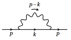
Figure 5: The gauge boson correction to the fermion propagator.

Appendix C Coupling between the Gauge field and nematic field

We start from the theory of the Fermi surface coupled to the Chern-Simons gauge field,

$$\mathcal{S}= \int d^{2}rdt~{}\Psi^{\dagger}(\bm{r},t)[D_{t}+\frac{1}{2m}\bm{D}^{2}+\frac{M_{1}}{2m}(D_{x}^{2}-D_{y}^{2})+\frac{M_{2}}{2m}(2D_{x}D_{y})]\Psi(\bm{r},t)$$

$$+\frac{1}{8\pi}\int d^{2}rdt~{}\epsilon^{\mu\nu\rho}\delta a_{\mu}\partial_{\nu}\delta a_{\rho}+\int d^{2}rd^{2}r^{\prime}dtV(\bm{r-r^{\prime}})\delta\rho(\bm{r},t)\delta\rho(\bm{r^{\prime}},t)$$ (87)

where $D_{\mu}=\partial_{\mu}+\delta a_{\mu}$. The external magnetic field is screened by the Chern-Simons flux while $\delta a_{i}$ represent the gauge fluctuation. In this mean-field level, the average flux felt by the composite fermion is zero so the CF is in the Fermi liquid state. If we consider gauge fluctuation to the quadratic order, we obtain the effective polarization for the gauge field

$$\mathcal{S}_{a}=-\frac{1}{2}\int_{\bm{q},\omega}\delta a_{\mu}(\bm{q},\omega)\Pi_{\mu\nu}(\bm{q},\omega)\delta a_{\nu}(\bm{-q},-\omega)$$ (88)

where

$$\Pi_{\mu\nu}=\frac{1}{2\pi}\begin{pmatrix}q^{2}\Pi_{0}&q_{x}\omega\Pi_{0}+iq_{y}/2&q_{y}\omega\Pi_{0}-iq_{x}/2\\ q_{x}\omega\Pi_{0}-iq_{y}/2&\omega^{2}\Pi_{0}-q_{y}^{2}(\Pi_{2}+V(\bm{q}))&q_{y}q_{x}(\Pi_{2}+V(\bm{q}))-i\omega/2\\ q_{y}\omega\Pi_{0}+iq_{x}/2&q_{y}q_{x}(\Pi_{2}+V(\bm{q}))+i\omega/2&\omega^{2}\Pi_{0}-q_{x}^{2}(\Pi_{2}+V(\bm{q}))\end{pmatrix}$$ (89)

with

$$\Pi_{0}(\bm{q},\omega) =\frac{m}{q^{2}}-\frac{i|\omega|}{\sqrt{{\bar{\rho}}}|q|^{3}},$$ (90)

$$\Pi_{2}(\bm{q},\omega) =\frac{1}{m}+\gamma\frac{i|\omega|\sqrt{{\bar{\rho}}}}{|q|^{3}},$$ (91)

where ${\bar{\rho}}$ is the electron density.

The linear, parity-even, coupling between the nematic field and the gauge field, i.e. the quadrupolar coupling between nematic fluctuations and gauge fields, at mean field level has the form,

$$\mathcal{S}_{a,M}[\bm{M},\delta a_{\mu}]=-\frac{1}{2}\int_{\bm{q},\omega}M_{i}(\bm{q},\omega)T_{i\nu}(\bm{q},\omega)\delta a_{\nu}(\bm{q},\omega)$$ (92)

where

$$T(\bm{q},\omega)= \frac{\Pi_{2}(\bm{q},\omega)m}{2\pi}\begin{pmatrix}q_{x}^{2}-q_{y}^{2}&q_{x}\omega&-q_{y}\omega\\ 2q_{x}q_{y}&\omega q_{y}&q_{x}\omega\end{pmatrix},$$

$$\Pi_{2}(\bm{q},\omega)= \gamma\frac{i|\omega|\sqrt{{\bar{\rho}}}}{|q|^{3}}$$ (93)

where we used the overdamped form of $\Pi_{2}(\bm{q},\omega)$, for $1\gg\frac{\omega}{qv_{F}}\gg q^{2}$.

We also have the coupling between the nematic order parameter and the Chern-Simons gauge fields,

$$\mathcal{S}_{a,M,a}[\delta a_{\mu},\bm{M}]=-\frac{1}{2}\int_{\bm{q},\omega}\delta a_{\mu}(\bm{q},\omega)V_{\mu\nu}[\bm{M}]\delta a_{\nu}(\bm{-q},-\omega)$$ (94)

$$V_{\mu\nu}[\bm{M}]=\frac{\Pi_{0}(\bm{q},\omega)}{2\pi}\begin{pmatrix}\frac{M_{1}}{2}(q_{x}^{2}-q_{y}^{2})&(M_{1}q_{x}+M_{2}q_{y})\omega&(-M_{2}q_{y}+M_{2}q_{x})\omega\\ (M_{1}q_{x}+M_{2}q_{y})\omega&M_{1}\omega^{2}&M_{2}\omega^{2}\\ (-M_{2}q_{y}+M_{2}q_{x})\omega&M_{2}\omega^{2}&-M_{1}\omega^{2}\end{pmatrix}$$ (95)

This parity-even term represents the coupling of the gauge fields to the nematic fluctuations as a local fluctuation of the spatial metric.

Appendix D Details of calculation of the Berry phase term

In this section, we show the detailed calculation of the Berry phase term whose Feynman diagram is shown in Fig.2. We obtained a similar term in the case of the FQH in Ref.[You et al., 2014]. The Berry phase term is obtained once we integrate out the gauge fluctuation and expand the theory in quadratic level. Here, we start from the gauge-nematic order parameter theory. Here we choose the temporal gauge $a_{0}=0$, and set $m=1$ (which we will restore back later).

$$\mathcal{S}=-\int_{\bm{q},\omega}\frac{1}{2}\delta a_{i}(\bm{q},\omega)[\Pi_{ij}+t^{1}_{ij}(\omega^{2}\Pi_{0})M_{1}+t^{2}_{ij}(\omega^{2}\Pi_{0})M_{2})]\delta a_{j}(\bm{-q},-\omega)$$

$$\Pi^{-1}=\frac{\begin{pmatrix}\omega^{2}\Pi_{0}-q_{x}^{2}\Pi_{2}&-q_{x}q_{y}\Pi_{2}-i\omega/2\\ -q_{x}q_{y}\Pi_{2}+i\omega/2&\omega^{2}\Pi_{0}-q_{y}^{2}\Pi_{2}\end{pmatrix}}{\omega^{4}\Pi_{0}^{2}-q^{2}\omega^{2}\Pi_{0}\Pi_{2}-\omega^{2}/4}$$ (96)

Since we are looking at the limit $|\frac{\omega}{v_{F}q}|<1$, we only keep the order of $O(\frac{\omega}{v_{F}q})$ for the damping part in the gauge boson propagator and drop terms like $(\frac{\omega}{v_{F}q})^{2}$. Afterwards, the inverse of the polarization tensor is,

$$\Pi^{-1}=-\frac{\begin{pmatrix}-q_{x}^{2}\Pi_{2}&-q_{x}q_{y}\Pi_{2}-i\omega/2\\ -q_{x}q_{y}\Pi_{2}+i\omega/2&-q_{y}^{2}\Pi_{2}\end{pmatrix}}{q^{2}\omega^{2}\Pi_{0}\Pi_{2}+\omega^{2}/4}$$

$$\Pi_{0}(\bm{q},\omega)=\frac{m}{q^{2}},~{}~{}\Pi_{2}(\bm{q},\omega)=\gamma\frac{i|\omega|\sqrt{{\bar{\rho}}}}{|q|^{3}},$$ (97)

Here we temporarily use units in which $m=1$ for convenience. Then the effective theory for the nematic order parameters can be obtained as

$$(-i)\frac{\delta\mathcal{S}}{\delta M_{i}\delta M_{j}}(\Omega,\bm{Q})=$$

$$i\textrm{Tr}\int_{\bm{q},\omega}~{}\Pi^{-1}(\omega,\bm{q})\omega^{2}\Pi_{0}t_{i}\Pi^{-1}(\omega+\Omega,\bm{q+Q})\omega^{2}\Pi_{0}t_{j}$$

$$=i\Omega/2\epsilon^{ij}~{}\int_{\bm{q},\omega}~{}\frac{\Pi_{2}q^{2}}{\Pi_{2}q^{2}+q^{2}/4}\frac{1}{\Pi_{2}q^{2}+q^{2}/4}$$ (98)

where $t_{1}=\sigma_{3}$ and $t_{2}=\sigma_{1}$.

Thus the anti-symmetric part of the effective theory of the nematic order parameters is

$$\mathcal{L}^{M}_{ij}=\chi\epsilon^{ij}M_{i}(\Omega,\bm{Q})(i\Omega)M_{j}(-\Omega,-\bm{Q})$$ (99)

where $\chi=\frac{2}{3\pi}\bar{\Lambda}$, and $\bar{\Lambda}$ is the frequency cut off. After putting back in the electron mass, we have $\chi=\frac{2}{3\pi}\bar{\Lambda}m$.

Appendix E Details of calculations of the Wen-Zee term

First, we calculate the parity-even part of the Wen-Zee term where the diagram has one gauge leg and one nematic leg (see Fig.3) We use the temporal gauge $a_{0}=0$ and take units in which $m=1$, and find

$$(-i)\frac{\delta\mathcal{S}}{\delta M_{l}\delta a_{k}}=\langle a_{m}\omega^{2}\Pi_{0}t^{mn}_{l}a_{n}a_{m}\omega^{2}\Pi_{0}Q^{mi}_{k}M_{i}\rangle$$ (100)

where

$$T^{-1}_{mi}=\langle a_{m}M_{i}\rangle(\bm{q},\omega)=\frac{\begin{pmatrix}q_{x}\omega&-q_{y}\omega\\ \omega q_{y}&q_{x}\omega\end{pmatrix}_{mi}}{\Pi_{2}q^{2}\omega^{2}},$$ (101)

with the notation $Q_{x}=I,Q_{y}=i\sigma_{2}$, and

$$-i\frac{\delta\mathcal{S}}{\delta M_{l}\delta a_{k}}(\bm{p},\Omega) =i\int_{\bm{q},\omega}~{}\textrm{Tr}\Big{[}(\omega^{2}\Pi_{0})^{2}\Pi^{-1}(\omega-\Omega/2,\bm{q-Q/2})t_{l}T^{-1}(\omega+\Omega/2,\bm{q+Q/2})Q_{k}\Big{]}$$

$$=\begin{pmatrix}p_{x}\Omega&-p_{y}\Omega\\ \Omega p_{y}&p_{x}\Omega\end{pmatrix}_{lk}\int_{\bm{p},\omega}\frac{1}{2q(\Pi_{2}q^{3}+q^{3}/4)}$$

$$=\frac{1}{6\pi\sqrt{3}}(\frac{\bar{\Lambda}}{{\bar{\rho}}})^{1/3}\begin{pmatrix}p_{x}\Omega&-p_{y}\Omega\\ \Omega p_{y}&p_{x}\Omega\end{pmatrix}_{lk}$$ (102)

Restoring the mass back, we have

$$-i\frac{\delta\mathcal{S}}{\delta M_{l}\delta a_{k}}(\bm{p},\Omega)=\frac{1}{6\pi\sqrt{3}}(\frac{\bar{\Lambda}m}{{\bar{\rho}}})^{1/3}\begin{pmatrix}p_{x}\Omega&-p_{y}\Omega\\ \Omega p_{y}&p_{x}\Omega\end{pmatrix}_{lk}$$ (103)

To calculate the cubic level of the Wen-Zee term where the diagram has one gauge field external leg and two nematic fields external legs (shown in Fig. 4).We will choose the axial gauge where $a_{0}=0$ (and use units which the effective mass is $m$=1), to find

$$-i\frac{\delta\mathcal{S}}{\delta M_{h}\delta M_{l}\delta a_{k}}=-\langle a_{m}\omega^{2}\Pi_{0}\sigma^{mn}_{h}a_{n}a_{m}\omega^{2}\Pi_{0}\sigma^{mn}_{l}a_{n}a_{m}\omega^{2}\Pi_{0}Q^{mi}_{k}M_{i}\rangle$$ (104)

Similarly,

$$(-i)\frac{\delta\mathcal{S}}{\delta M_{h}\delta M_{l}\delta a_{k}}(\Omega_{1},\Omega_{2};\bm{p_{1}},\bm{p_{2}})$$

$$=-\int_{\bm{q},\omega}~{}\textrm{Tr}\Big{[}\Pi^{-1}(\omega,\bm{q})(\omega^{2}\Pi_{0}\sigma_{h})\Pi^{-1}(\omega+\Omega_{1},\bm{q+p_{1}})(\omega^{2}\Pi_{0}\sigma_{l})T^{-1}(\omega+\Omega_{1}+\Omega_{2},\bm{q+p_{1}+p_{2}})(\omega^{2}\Pi_{0}Q_{k})\Big{]}$$

$$=\epsilon^{hl}\epsilon^{\nu\mu k}p_{1}^{\nu}(p_{1}^{\mu}+p_{2}^{\mu})\int_{\bm{q},\omega}~{}\Big{[}\frac{|\omega|q^{2}}{8q(\Pi_{2}q^{3}+q^{3}/4)^{2}}+\frac{\Pi_{2}q^{3}}{8q(\Pi_{2}q^{3}+q^{3}/4)^{2}}\Big{]}$$

$$=\frac{1}{6\pi\sqrt{3}}\Big{[}\left(\frac{\bar{\Lambda}}{{\bar{\rho}}}\right)^{1/3}+\frac{\bar{\Lambda}}{{\bar{\rho}}}\Big{]}\epsilon^{hl}\epsilon^{\nu\mu k}p_{1}^{\nu}(p_{1}^{\mu}+p_{2}^{\mu})$$ (105)

Restoring the mass back, we find the effective theory as

$$(-i)\frac{\delta\mathcal{S}}{\delta M_{h}\delta M_{l}\delta a_{k}}(\Omega_{1},\Omega_{2};\bm{p_{1}},\bm{p_{2}})$$

$$=\frac{1}{6\pi\sqrt{3}}\Big{[}\left(\frac{\bar{\Lambda}m}{{\bar{\rho}}}\right)^{1/3}+\frac{\bar{\Lambda}m}{{\bar{\rho}}}\Big{]}\epsilon^{hl}\epsilon^{\nu\mu k}p_{1}^{\nu}(p_{1}^{\mu}+p_{2}^{\mu})$$ (106)

Similar to the calculation of the Berry phase term by Ward Identity, the Wen-Zee term can also be derived from the Ward Identity. The nematic order parameter modifies the local geometry metric of the Maxwell term and couples to the bilinear of the Chern-Simons gauge fields. At this level, we can integrate out the gauge fields and perform the loop expansion of the nematic fields at the cubic level.

$$\langle T_{1}T_{2}T_{xy}\rangle (\bm{p}_{1},\bm{p}_{2},\Omega_{1},\Omega_{2})=$$

$$-\int_{\bm{k},\omega}\textrm{Tr}\Big{[}\Pi^{-1}(\bm{k},\omega)(\Pi_{0}\omega^{2})\sigma_{z}\Pi^{-1}(\bm{k+p_{1}},\omega+\Omega_{1})(\Pi_{0}\omega^{2})\sigma_{z}\Pi^{-1}(\bm{k+p_{1}+p_{2}},\omega+\Omega_{1})(\Pi_{0}\omega^{2})\sigma_{+}\Big{]}$$ (107)

By taking advantage of the Ward Identity, we find

$$m\partial_{0}J_{x}+\partial_{x}T_{xx}+\partial_{y}T_{yx}=\delta b\cdot J_{y}$$

$$m\partial_{0}J_{y}+\partial_{x}T_{xy}+\partial_{y}T_{yy}=-\delta b\cdot J_{x}$$ (108)

We can set up several relations between the Wen-Zee term and the terms cubic in nematic order parameters,

$$m\langle T_{1}(\bm{r}_{1})T_{2}(\bm{r}_{2})\partial_{0}J_{x}(\bm{r}_{3})\rangle+\langle T_{1}(\bm{r}_{1})T_{2}(\bm{r}_{2})\partial_{x}T_{xx}(\bm{r}_{3})\rangle+\langle T_{1}(\bm{r}_{1})T_{2}(\bm{r}_{2})\partial_{y}T_{yx}(\bm{r}_{3})\rangle=2\langle T_{1}(\bm{r}_{1})T_{2}(\bm{r}_{2})\delta\rho(\bm{r}_{3})J_{y}(\bm{r}_{3})\rangle$$

$$m\langle T_{1}(\bm{r}_{1})T_{2}(\bm{r}_{2})\partial_{0}J_{y}(\bm{r}_{3})\rangle+\langle T_{1}(\bm{r}_{1})T_{2}(\bm{r}_{2})\partial_{x}T_{xy}(\bm{r}_{3})\rangle+\langle T_{1}(\bm{r}_{1})T_{2}(\bm{r}_{2})\partial_{y}T_{yy}(\bm{r}_{3})\rangle=-2\langle T_{1}(\bm{r}_{1})T_{2}(\bm{r}_{2})\delta\rho(\bm{r}_{3})J_{x}(\bm{r}_{3})\rangle$$ (109)

It is straightforward to see that the correlators on the right hand sides are actually zero. Also, the further calculation shows that $\langle T_{1}(\bm{r}_{1})T_{2}(\bm{r}_{2})\partial_{x}T_{xx}(\bm{r}_{3})\rangle$ and $\langle T_{1}(\bm{r}_{1})T_{2}(\bm{r}_{2})\partial_{y}T_{yy}(\bm{r}_{3})\rangle$ does not generate any anti-symmetric term at the leading order ($O(q^{3})$). Now the identities become,

$$m\langle T_{1}(\bm{r}_{1})T_{2}(\bm{r}_{2})\partial_{0}J_{x}(\bm{r}_{3})\rangle=-\langle T_{1}(\bm{r}_{1})T_{2}(\bm{r}_{2})\partial_{y}T_{yx}(\bm{r}_{3})\rangle$$

$$m\langle T_{1}(\bm{r}_{1})T_{2}(\bm{r}_{2})\partial_{0}J_{y}(\bm{r}_{3})\rangle=-\langle T_{1}(\bm{r}_{1})T_{2}(\bm{r}_{2})\partial_{x}T_{xy}(\bm{r}_{3})\rangle$$ (110)

We have

$$\langle T_{i}T_{j}\partial_{y}T_{yx}\rangle(\bm{p_{1},p_{2}},\omega_{1},\omega_{2})=s\epsilon^{ij}\omega_{1}(\omega_{1}+\omega_{2})(-p^{y}_{1}-p^{y}_{2})-s\epsilon^{ij}\omega_{1}(\omega_{1}+\omega_{2})p^{y}_{1}$$

$$\langle T_{i}T_{j}\partial_{x}T_{xy}\rangle(\bm{p_{1},p_{2}},\omega_{1},\omega_{2})=-s\epsilon^{ij}\omega_{1}(\omega_{1}+\omega_{2})(-p^{x}_{1}-p^{x}_{2})+s\epsilon^{ij}\omega_{1}(\omega_{1}+\omega_{2})p^{x}_{1}$$ (111)

Thus, the Wen-Zee term has the form

$$\langle T_{i}T_{j}J_{x}\rangle(\bm{p_{1},p_{2}},\omega_{1},\omega_{2})=\frac{s}{m}\epsilon^{ij}\omega_{1}(-p^{y}_{1}-p^{y}_{2})-s\epsilon^{ij}(-\omega_{1}-\omega_{2})p^{y}_{1}$$

$$\langle T_{i}T_{j}J_{y}\rangle(\bm{p_{1},p_{2}},\omega_{1},\omega_{2})=-\frac{s}{m}\epsilon^{ij}\omega_{1}(-p^{x}_{1}-p^{x}_{2})+s\epsilon^{ij}(-\omega_{1}-\omega_{2})p^{x}_{1}$$ (112)

By taking advantage of the current conservation relation,

$$\partial_{\mu}J_{\mu}=0$$ (113)

We obtain

$$\langle T_{i}T_{j}J_{0}\rangle(\bm{p_{1},p_{2}},\omega_{1},\omega_{2})= \frac{s}{m}\epsilon^{ij}p^{y}_{1}(-p^{x}_{1}-p^{x}_{2})$$

$$- s\epsilon^{ij}(-p^{y}_{1}-p^{y}_{2})p^{x}_{1}$$ (114)

Where the coefficient $\frac{s}{m}$ is obtained to be

$$\frac{s}{m}=\frac{1}{6\pi\sqrt{3}}\Big{[}\left(\frac{\bar{\Lambda}m}{{\bar{\rho}}}\right)^{1/3}+\frac{\bar{\Lambda}m}{{\bar{\rho}}}\Big{]}$$ (115)

Thus, we finally obtain that the Wen-Zee term $\mathcal{L}_{WZ}$ of the effective Lagrangian is

$$\mathcal{L}_{WZ}=\frac{1}{6\pi\sqrt{3}}\Big{[}\left(\frac{\bar{\Lambda}m}{{\bar{\rho}}}\right)^{1/3}+\frac{\bar{\Lambda}m}{{\bar{\rho}}}\Big{]}\ ~{}\epsilon^{\mu\nu\rho}\omega_{\mu}^{Q}\partial_{\nu}A_{\rho}$$ (116)

Appendix F Nematic correlators

The self-energy of the composite fermion close to the Fermi surface is,

$$\Sigma_{s}(\omega)=-i2\sqrt{3}\;\textrm{sign}(\omega)(\frac{\beta\omega}{4\pi})^{2/3}$$ (117)

The Fermi surface is softened by the gauge boson and thus no longer well defined. Here we check the correction from the self-energy to of the nematic correlator.

The nematic correlator of the Fermi surface without self-energy correction is shown in the Feynman diagram of Fig.1, and it is given by

$$-i\frac{\delta S}{\delta M_{1}\delta M_{1}} =\langle T_{1}T_{1}\rangle_{0}(\bm{p},\Omega)$$

$$=-i\int_{\bm{k},\omega}~{}g(\bm{k+p},\omega+\Omega)\frac{(k_{x}^{2}-k_{y}^{2})}{2m}g(\bm{k},\omega)\frac{(k_{x}^{2}-k_{y}^{2})}{2m}$$

$$=-i\int_{\bm{k},\omega}~{}\frac{1}{4m^{2}}\frac{(k_{x}^{2}-k_{y}^{2})}{\omega+\Omega-((\bm{k+p})^{2}+k_{F}^{2})/2m+i\eta\;\textrm{sign}(\omega+\Omega)}~{}\frac{(k_{x}^{2}-k_{y}^{2})}{\omega-(\bm{k}^{2}+k_{F}^{2})/2m+i\eta\;\textrm{sign}(\omega)}$$

$$=k_{F}^{4}/(4\pi m)-\cos^{2}(2\theta_{p})\frac{k_{F}^{3}}{2\pi}(i\Omega/p)-\sin^{2}(2\theta_{p})\frac{k_{F}^{2}m}{2\pi}(\Omega/p)^{2}$$ (118)

If we only look into the leading self-energy correction, it is the sum of the diagrams in Fig. 6,

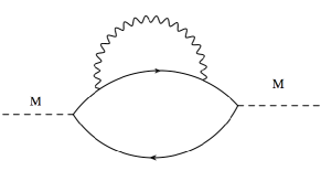
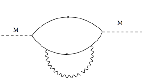
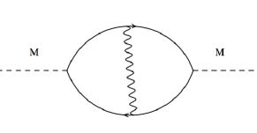
Figure 6: Leading corrections from gauge field fluctuations to the nematic correlators: a) and b) composite fermion self-energy corrections, and c) vertex correction.

$$\langle T_{1}T_{1}\rangle_{1}(\bm{p},\Omega) =$$

$$-i\int_{\bm{k},\omega}~{}(k_{x}^{2}-k_{y}^{2})^{2}/(4m^{2})[g(\bm{k+p},\omega+\Omega)\Sigma_{s}(\omega)g^{2}(\bm{k},\omega)+g^{2}(\bm{k+p},\omega+\Omega)\Sigma_{s}(\omega+\Omega)g(\bm{k},\omega)]$$ (119)

Here the self-energy $\Sigma_{s}(\omega)$ only affects the fermions near the Fermi surface where $k\sim k_{F}$, Take advantage of the identity

$$g(\bm{k+p},\omega+\Omega)\Sigma_{s}(\omega)g^{2}(\bm{k},\omega)=-\frac{\Sigma_{s}(\omega)}{\Omega-\bm{k}\cdot\bm{p}/2m}[g^{2}(\bm{k},\omega)-g(\bm{k+p},\omega+\Omega)g(\bm{k},\omega)]$$

$$g^{2}(\bm{k+p},\omega+\Omega)\Sigma_{s}(\omega+\Omega)g(\bm{k},\omega)=\frac{\Sigma_{s}(\omega+\Omega)}{\Omega-\bm{k}\cdot\bm{p}/2m}[g^{2}(\bm{k+p},\omega+\Omega)-g(\bm{k+p},\omega+\Omega)g(\bm{k},\omega)]$$ (120)

We can rewrite the integral as

$$\langle T_{1}T_{1}\rangle_{1}(\bm{p},\Omega)=-i\int_{\bm{k},\omega}~{}(k_{x}^{2}-k_{y}^{2})^{2}/(4m^{2})\frac{\Sigma_{s}(\omega)-\Sigma_{s}(\omega+\Omega)}{\Omega-\bm{k}\cdot\bm{p}/2m}g(\bm{k+p},\omega+\Omega)g(\bm{k},\omega)$$ (121)

In the same way, the other nematic correlators can be written as

$$\langle T_{2}T_{2}\rangle_{1}(\bm{p},\Omega) =-i\int_{\bm{k},\omega}~{}(2k_{x}k_{y})^{2}/(4m^{2})\frac{\Sigma_{s}(\omega)-\Sigma_{s}(\omega+\Omega)}{\Omega-\bm{k}\cdot\bm{p}/2m}g(\bm{k+p},\omega+\Omega)g(\bm{k},\omega)$$

$$\langle T_{2}T_{1}\rangle_{1}(\bm{p},\Omega) =-i\int_{\bm{k},\omega}~{}(k_{x}^{2}-k_{y}^{2})(2k_{x}k_{y})/(4m^{2})\frac{\Sigma_{s}(\omega)-\Sigma_{s}(\omega+\Omega)}{\Omega-\bm{k}\cdot\bm{p}/2m}g(\bm{k+p},\omega+\Omega)g(\bm{k},\omega)$$ (122)

Here we first calculate $\langle T_{1}T_{1}\rangle_{1}$,

$$\langle T_{1}T_{1}\rangle_{1} (\bm{p},\Omega)=$$

$$=-i\int_{\bm{k},\omega}~{} \frac{k^{4}\cos^{2}(2\theta)}{4m^{2}}\frac{\Sigma_{s}(\omega)-\Sigma_{s}(\omega+\Omega)}{\Omega-kp\cos(\theta-\theta_{p})/2m}\frac{1}{\omega+\Omega-(E(k)+kp\cos(\theta-\theta_{p})/2m)+i\eta\;\textrm{sign}(\omega+\Omega)}\frac{1}{\omega-E(k)+i\eta\;\textrm{sign}(\omega)}$$

where $E(k)=(k^{2}-k_{F}^{2})/2m$.

Since the self energy correction $\Sigma(\omega)$ only appears near the Fermi surface, we can replace $k/2m=v_{F}=k_{F}/2m$ in the calculation to simplified the problem. We can replace the integral $d\bm{k}=dE(k)d\theta~{}2m$,

$$\langle T_{1}T_{1}\rangle_{1}(\bm{p},\Omega)=$$

$$-i\int d\omega dE(k)d\theta~{}\frac{k_{F}^{4}\cos^{2}(2\theta)}{4m}\frac{\Sigma_{s}(\omega)-\Sigma_{s}(\omega+\Omega)}{\Omega-v_{F}p\cos(\theta-\theta_{p})}\frac{1}{\omega+\Omega-(E(k)+v_{F}p\cos(\theta-\theta_{p}))+i\eta\;\textrm{sign}(\omega+\Omega)}\frac{1}{\omega-E(k)+i\eta\;\textrm{sign}(\omega)}$$

$$=\int d\omega d\theta~{}\frac{k_{F}^{4}\cos^{2}(2\theta)}{4m}\frac{\Sigma_{s}(\omega)-\Sigma_{s}(\omega+\Omega)}{(\Omega-v_{F}p\cos(\theta-\theta_{p}))^{2}}(\;\textrm{sign}(\omega)-\;\textrm{sign}(\omega+\Omega))$$ (124)

First, we look at the static limit $\Omega=0$. Then we have $\Sigma_{s}(\omega)-\Sigma_{s}(\omega+\Omega)=0$ and therefore the integral is zero. This indicates the leading order self-energy correction does not generate any constant term, and thus the mass term of the nematics remains unchanged by the imaginary part of self-energy.

Now we turn to the case when $\Omega$ is nonzero and take the limit $p\ll k_{F}$ and $\Omega\ll p$. The integral of $\theta$ can be done by contour integral, we take the leading order in regard of $\Omega/p$. Since we are only interested in the leading order behavior of the damping term, we calculate $\langle(T_{1}T_{1}+T_{2}T_{2})\rangle_{1}$ to simplify the calculation.

$$\langle T_{i}T_{i}\rangle_{1}(\bm{p},\Omega) =$$

$$=\int d\omega d\theta~{}\frac{k_{F}^{4}}{4m}\frac{\Sigma_{s}(\omega)-\Sigma_{s}(\omega+\Omega)}{(\Omega-v_{F}p\cos(\theta-\theta_{p}))^{2}}(\;\textrm{sign}(\omega)-\;\textrm{sign}(\omega+\Omega))$$

$$=\int d\omega~{}\frac{k_{F}^{4}}{4m}\frac{\Sigma_{s}(\omega)-\Sigma_{s}(\omega+\Omega)}{(v_{F}p)^{2}}(\;\textrm{sign}(\omega)-\;\textrm{sign}(\omega+\Omega))\frac{\Omega}{v_{F}p}\frac{1}{(1+(\Omega/v_{F}p)^{2})^{3/2}}$$

$$\approx\int d\omega~{}\frac{k_{F}^{4}}{4m}\frac{\Sigma_{s}(\omega)-\Sigma_{s}(\omega+\Omega)}{(v_{F}p)^{2}}(\;\textrm{sign}(\omega)-\;\textrm{sign}(\omega+\Omega))\frac{\Omega}{v_{F}p}$$

$$=~{}\frac{k_{F}^{4}\sqrt{3}}{2m}\frac{\beta^{2/3}\Omega^{5/3}}{(v_{F}p)^{2}}\frac{\Omega}{v_{F}p}$$ (125)

The leading order damping upon the self-energy correction is $(\Omega)^{8/3}/q^{3}$, which is highly irrelevant so we can ignore it. However, one might worry that $\langle T_{1}T_{1}\rangle_{1}$ could contain a singular damping term which could cancel when added to $\langle T_{2}T_{2}\rangle_{1}$. If this cancellation happened, then the damping coefficient $\langle T_{1}T_{1}\rangle_{1}$ would be a function of $\cos(4\theta_{p})$. We can then choose $\theta_{p}=0$ and calculate $\langle T_{1}T_{1}\rangle_{1}$ to check the leading damping term. The leading order of damping for $\langle T_{1}T_{1}\rangle_{1}(\theta_{p}=0)$ is of order $\Omega^{5/3}/q^{2}$, which is still irrelevant compared to the damping term.

In conclusion, the leading order self-energy correction does not change the leading order behavior of the nematic transition. In sum, the nematic polarization tensor is

$$\langle T_{i}T_{j}\rangle(\bm{p},\Omega)=$$

$$\begin{pmatrix}k_{F}^{4}/(4\pi m)-\cos^{2}(2\theta_{p})\frac{k_{F}^{3}}{2\pi}(i\Omega/p)-\sin^{2}(2\theta_{p})\frac{k_{F}^{2}m}{2\pi}(\Omega/p)^{2}&\sin(2\theta_{p})\cos(2\theta_{p})\frac{k_{F}^{3}}{2\pi}(i\Omega/p)\\ \sin(2\theta_{p})\cos(2\theta_{p})\frac{k_{F}^{3}}{2\pi}(i\Omega/p))&k_{F}^{4}/(4\pi m)-\sin^{2}(2\theta_{p})\frac{k_{F}^{3}}{2\pi}(i\Omega/p)-\cos^{2}(2\theta_{p})\frac{k_{F}^{2}m}{2\pi}(\Omega/p)^{2}\end{pmatrix}$$ (126)

Appendix G Vertex correction for nematic polarization tensor

In this section, we show the vertex correction for the nematic polarization tensor is irrelevant in our theory (shown in Fig.6c)

$$\langle T_{1}T_{1}\rangle_{v}(\bm{p},\Omega)+\langle T_{2}T_{2}\rangle_{v}(\bm{p},\Omega)=$$

$$-i\int_{\bm{k},\bm{q},\omega,\nu}~{}\frac{k^{6}}{4m^{4}}g(\bm{k+p},\omega+\Omega)g(\bm{k},\omega)g(\bm{k+p+q},\omega+\Omega+\nu)g(\bm{k+q},\omega+\Omega)D_{11}(\bm{q},\nu)$$ (127)

To proceed, we first calculate the vertex,

$$\Gamma(\bm{k},\bm{p},\omega,\Omega) =$$

$$-i\int_{\bm{q},\nu}~{}g(\bm{k+p+q},\omega+\Omega+\nu)g(\bm{k+q},\omega+\Omega)D_{11}(\bm{q},\nu)$$

$$-i\int_{\bm{q},\nu}~{}\frac{|q_{v}|}{(\omega+\Omega+\nu-(E(k)+v_{F}q_{l}+v_{F}p\cos(\theta-\theta_{p})+q_{v}p\sin(\theta-\theta_{p}))+i\eta\;\textrm{sign}(\omega+\Omega+\nu))}$$

$$\times\frac{1}{(a|\nu|+b|q_{v}|^{3})}~{}\frac{1}{\omega+\nu-(E(k)+v_{F}q_{l})+i\eta\;\textrm{sign}(\omega+\nu)}$$ (128)

where $q_{v}=q\sin(\theta-\theta_{q}),q_{l}=q\cos(\theta-\theta_{q})$. $a=2m\sqrt{3}$ and $b=1/4$ are constants which we will take as unity for simplicity since we are only interested in scaling behaviors. Taking the integral $q_{l}$ first, we find

$$\Gamma(\bm{k},\bm{p},\omega,\Omega) =$$

$$-i\int_{q_{v},\nu}~{}\frac{|q_{v}|(\;\textrm{sign}(\omega+\Omega+\nu)-\;\textrm{sign}(\omega+\nu))}{(\Omega-v_{F}p\cos(\theta-\theta_{p})+q_{v}p\sin(\theta-\theta_{p}))(a|\nu|+b|q_{v}|^{3})}$$

$$\sim-i\int_{q_{v}}~{}\frac{|q_{v}|}{\Omega-v_{F}p\cos(\theta-\theta_{p})+q_{v}p\sin(\theta-\theta_{p})}\Big{(}\ln(1+\frac{|\omega+\Omega|}{|q_{v}|^{3}})\;\textrm{sign}(\omega+\Omega)-\ln(1+\frac{|\omega|}{|q_{v}|^{3}})\;\textrm{sign}(\omega)\Big{)}$$ (129)

It is obvious that when $\Omega=0$, this expression is vanishes. Thus the vertex correction does not contribute to the mass term of the polarization tensor.

Now we turn to the damping term in the vertex corrections to the polarization tensor,

$$\langle T_{i}T_{i}\rangle_{v}(\bm{p},\Omega) =$$

$$-i\int_{q_{v},\bm{k},\omega}~{}\frac{|q_{v}|}{\Omega-v_{F}p\cos(\theta-\theta_{p})+q_{v}p\sin(\theta-\theta_{p})}\Big{(}\ln(1+\frac{|\omega+\Omega|}{|q_{v}|^{3}})\;\textrm{sign}(\omega+\Omega)-\ln(1+\frac{|\omega|}{|q_{v}|^{3}})\;\textrm{sign}(\omega)\Big{)}$$

$$\times\frac{k^{6}}{4m^{4}}\Big{(}\omega+\Omega-E(k)-v_{F}p\cos(\theta-\theta_{p})+i\eta\;\textrm{sign}(\omega+\Omega))^{-1}(\omega-E(k)+i\eta\;\textrm{sign}(\omega)\Big{)}^{-1}$$ (130)

As the gauge field correction only affects the fermion propagator near the Fermi surface, we can take $\frac{k^{6}}{4m^{4}}=\frac{k_{F}^{6}}{4m^{4}}$ and take this constant aside. We can then replace the integral over $d\bm{k}=dE(k)d\theta~{}2m$ and integrate over $dE(k)$ first,

$$\langle T_{i}T_{i}\rangle_{v}(\bm{p},\Omega)\sim\int_{q_{v},\theta,\omega}~{} \frac{|q_{v}|}{\Omega-v_{F}p\cos(\theta-\theta_{p})+q_{v}p\sin(\theta-\theta_{p})}\Big{(}\ln(1+\frac{|\omega+\Omega|}{|q_{v}|^{3}})\;\textrm{sign}(\omega+\Omega)-\ln(1+\frac{|\omega|}{|q_{v}|^{3}})\;\textrm{sign}(\omega)\Big{)}$$

$$\times\frac{\;\textrm{sign}(\omega+\Omega)-\;\textrm{sign}(\omega)}{\Omega-v_{F}p\cos(\theta-\theta_{p})}$$

$$\sim\int_{q_{v},\theta}~{}\int_{0}^{\Omega}d\omega ~{}\frac{|q_{v}|}{\Omega-v_{F}p\cos(\theta-\theta_{p})+q_{v}p\sin(\theta-\theta_{p})}\ln(1+\frac{|\omega|}{|q_{v}|^{3}})\frac{1}{\Omega-v_{F}p\cos(\theta-\theta_{p})}$$ (131)

By the change of variables $l=\omega/\Omega$, we get

$$\langle T_{i}T_{i}\rangle_{v}(\bm{p},\Omega)\sim\int_{q_{v},\theta}~{}\int_{0}^{1}dl~{}\frac{\Omega|q_{v}|}{\Omega-v_{F}p\cos(\theta-\theta_{p})+q_{v}p\sin(\theta-\theta_{p})}\ln(1+\Omega\frac{|l|}{|q_{v}|^{3}})\frac{1}{\Omega-v_{F}p\cos(\theta-\theta_{p})}$$ (132)

Performing the $\theta$ integral (and take $v_{F}=1$ to simplify the expression), we find

$$\langle T_{i}T_{i}\rangle_{v}(\bm{p},\Omega)\sim\int_{q_{v}}~{}\int_{0}^{1}dl~{}\frac{\Omega|q_{v}|}{p^{2}}\frac{\Omega}{p}\ln(1+\Omega\frac{|l|}{|q_{v}|^{3}})\frac{1}{(1-(\Omega/p)^{2})\sqrt{1+(q_{v}/v_{f})^{2}-(\Omega/p)^{2}}}$$ (133)

Since we are looking at the fermion near the Fermi surface, $q_{v}$ shall have a cut off which is smaller than $v_{f}$. Once we assume $q_{v}/v_{F}<1$,

$$\langle T_{i}T_{i}\rangle_{v}(\bm{p},\Omega)\sim\int^{\Lambda}_{0}dq_{v}~{}\int_{0}^{1}dl~{}\frac{\Omega|q_{v}|}{p^{2}}\frac{\Omega}{p}\ln(1+\Omega\frac{|l|}{|q_{v}|^{3}})\frac{1}{(1-(\Omega/p)^{2})\sqrt{1-(\Omega/p)^{2}}}$$ (134)

where $\Lambda$ is the UV momentum cut off for $q_{v}$, integrate over $q_{v}$ and ignore the numerical constant,

$$\langle T_{i}T_{i}\rangle_{v}(\bm{p},\Omega) \sim~{}\int_{0}^{1}dl~{}\frac{\Omega}{p^{2}}\frac{\Omega}{p}(\Omega l)^{2/3}\frac{1}{(1-(\Omega/p)^{2})\sqrt{1-(\Omega/p)^{2}}}$$

$$\sim~{}\int_{0}^{1}dl~{}\frac{\Omega^{8/3}}{p^{3}}(l)^{2/3}$$

From the above calculation, it is obvious that the damping term from the vertex correction is of higher order compared to $\frac{\Omega}{p}$. One might worry that $\langle T_{1}T_{1}\rangle_{v}$ contains some singular damping term which cancels when sum with $\langle T_{2}T_{2}\rangle_{v}$. If this cancellation happens, then the damping coefficient $\langle T_{1}T_{1}\rangle_{v}$ must be a function of $\cos(4\theta_{p})$. We can then choose $\theta_{p}=0$ and calculate $\langle T_{1}T_{1}\rangle_{v}$ to check the leading damping term. The leading order of damping for $\langle T_{1}T_{1}\rangle_{v}(\theta_{p}=0)$ is of order $\Omega^{5/3}/q^{2}$, which is still irrelevant compared to the damping term.

Thus, the vertex correction to the overdamped mode is irrelevant.

References

- Fradkin et al. (2010) E. Fradkin, S. A. Kivelson, M. J. Lawler, J. P. Eisenstein, and A. P. Mackenzie, Annual Review of Condensed Matter Physics 1, 153 (2010).
- Chaikin and Lubensky (1995) P. M. Chaikin and T. C. Lubensky, Principles of Condensed Matter Physics (Cambridge University Press, Cambridge, UK, 1995).
- de Gennes and Prost (1993) P. G. de Gennes and J. Prost, The Physics of Liquid Crystals (Oxford Science Publications/Clarendon Press, Oxford, UK, 1993).
- Kivelson et al. (1998) S. A. Kivelson, E. Fradkin, and V. J. Emery, Nature 393, 550 (1998).
- Fradkin and Kivelson (1999) E. Fradkin and S. A. Kivelson, Phys. Rev. B 59, 8065 (1999).
- Ando et al. (2002) Y. Ando, K. Segawa, S. Komiya, and A. N. Lavrov, Phys. Rev. Lett. 88, 137005 (2002).
- Hinkov et al. (2008) V. Hinkov, D. Haug, B. Fauqué, P. Bourges, Y. Sidis, A. Ivanov, C. Bernhard, C. T. Lin, and B. Keimer, Science 319, 597 (2008).
- Daou et al. (2010) R. Daou, J. Chang, D. LeBoeuf, O. Cyr-Choiniere, F. Laliberte, N. Doiron-Leyraud, B. J. Ramshaw, R. Liang, D. A. Bonn, W. N. Hardy, and L. Taillefer, Nature 463, 519 (2010).
- Lawler et al. (2010) M. J. Lawler, K. Fujita, J. Lee, A. R. Schmidt, Y. Kohsaka, C. K. Kim, H. Eisaki, S. Uchida, J. C. Davis, J. P. Sethna, and E.-A. Kim, Nature 466, 347 (2010).
- Chu et al. (2012) J.-H. Chu, H.-H. Kuo, J. G. Analytis, and I. R. Fisher, Science 337, 710 (2012).
- Borzi et al. (2007) R. A. Borzi, S. A. Grigera, J. Farrell, R. S. Perry, S. J. S. Lister, S. L. Lee, D. A. Tennant, Y. Maeno, and A. P. Mackenzie, Science 315, 214 (2007).
- Lilly et al. (1999a) M. P. Lilly, K. B. Cooper, J. P. Eisenstein, L. N. Pfeiffer, and K. W. West, Phys. Rev. Lett. 82, 394 (1999a).
- Du et al. (1999) R. R. Du, D. C. Tsui, H. L. Störmer, L. N. Pfeiffer, K. W. Baldwin, and K. W. West, Solid State Comm. 109, 389 (1999).
- Cooper et al. (2002) K. B. Cooper, M. P. Lilly, J. P. Eisenstein, L. N. Pfeiffer, and K. W. West, Phys. Rev. B 65, 241313 (2002).
- Cooper et al. (2003) K. B. Cooper, J. P. Eisenstein, L. N. Pfeiffer, and K. W. West, Phys. Rev. Lett. 90, 226803 (2003).
- Pollanen et al. (2015) J. Pollanen, K. B. Cooper, S. Brandsen, J. P. Eisenstein, L. N. Pfeiffer, and K. W. West, Phys. Rev. B 92, 115410 (2015).
- Fradkin et al. (2000) E. Fradkin, S. A. Kivelson, E. Manousakis, and K. Nho, Phys. Rev. Lett. 84, 1982 (2000).
- Cooper et al. (2001) K. B. Cooper, M. P. Lilly, J. P. Eisenstein, T. Jungwirth, L. N. Pfeiffer, and K. W. West, Sol. State Commun. 119, 89 (2001).
- Lilly et al. (1999b) M. P. Lilly, K. B. Cooper, J. P. Eisenstein, L. N. Pfeiffer, and K. W. West, Phys. Rev. Lett. 83, 824 (1999b).
- Pan et al. (1999) W. Pan, R. R. Du, H. L. Störmer, D. C. Tsui, L. N. Pfeiffer, K. W. Baldwin, and K. W. West, Phys. Rev. Lett. 83, 820 (1999).
- Samkharadze et al. (2016) N. Samkharadze, K. A. Schreiber, G. C. Gardner, M. J. Manfra, E. Fradkin, and G. A. Csathy, Nature Phys. 12, 191 (2016).
- Xia et al. (2010) J. Xia, V. Cvicek, J. P. Eisenstein, L. N. Pfeiffer, and K. W. West, Phys. Rev. Lett. 105, 176807 (2010).
- Xia et al. (2011) J. Xia, J. Eisenstein, L. Pfeiffer, and K. West, Nature Phys. 7, 845 (2011).
- Moessner and Chalker (1996) R. Moessner and J. T. Chalker, Phys. Rev. B 54, 5006 (1996).
- Koulakov et al. (1996) A. A. Koulakov, M. M. Fogler, and B. I. Shklovskii, Phys. Rev. Lett. 76, 499 (1996).
- Fogler et al. (1996) M. Fogler, A. Koulakov, and B. Shklovskii, Phys. Rev. B 54, 1853 (1996).
- MacDonald and M. P. A. Fisher (2000) A. H. MacDonald and M. P. A. Fisher, Phys. Rev. B 61, 5724 (2000).
- Stanescu et al. (2000) T. D. Stanescu, I. Martin, and P. Phillips, Phys. Rev. Lett. 84, 1288 (2000).
- Barci et al. (2002) D. G. Barci, E. Fradkin, S. A. Kivelson, and V. Oganesyan, Phys. Rev. B 65, 245319 (2002).
- Fogler (2002) M. M. Fogler, Int. J. Mod. Phys. B 16, 2924 (2002).
- Côté and Fertig (2000) R. Côté and H. A. Fertig, Phys. Rev. B 62, 1993 (2000).
- Lopatnikova et al. (2001) A. Lopatnikova, S. H. Simon, B. I. Halperin, and X.-G. Wen, Phys. Rev. B 64, 155301 (2001).
- Lawler and Fradkin (2004) M. J. Lawler and E. Fradkin, Phys. Rev. B 70, 165310 (2004).
- Emery et al. (2000) V. J. Emery, E. Fradkin, S. A. Kivelson, and T. C. Lubensky, Phys. Rev. Lett. 85, 2160 (2000).
- Vishwanath and Carpentier (2001) A. Vishwanath and D. Carpentier, Phys. Rev. Lett. 86, 676 (2001).
- Sondhi and Yang (2001) S. L. Sondhi and K. Yang, Phys. Rev. B 63, 054430 (2001).
- Fertig (1999) H. A. Fertig, Phys. Rev. Lett. 82, 3693 (1999).
- Rezayi and Haldane (2000) E. H. Rezayi and F. Haldane, Phys. Rev. Lett. 84, 4686 (2000).
- Mulligan et al. (2010) M. Mulligan, C. Nayak, and S. Kachru, Phys. Rev. B 82, 085102 (2010).
- You and Fradkin (2013) Y. You and E. Fradkin, Phys. Rev. B 88, 235124 (2013).
- You et al. (2014) Y. You, G. Y. Cho, and E. Fradkin, Phys. Rev. X 4, 041050 (2014).
- Haldane (2009) F. D. M. Haldane, ““Hall viscosity” and intrinsic metric of incompressible fractional Hall fluids,” (2009), unpublished, arXiv:0906.1854 .
- Haldane (2011) F. D. M. Haldane, Phys. Rev. Lett. 107, 116801 (2011).
- Yang (2013) K. Yang, Phys. Rev. B 88, 241105 (2013).
- Maciejko et al. (2013) J. Maciejko, B. Hsu, S. Kivelson, Y. Park, and S. Sondhi, Phys. Rev. B 88, 125137 (2013).
- Radzihovsky and Dorsey (2002) L. Radzihovsky and A. T. Dorsey, Phys. Rev. Lett. 88, 216802 (2002).
- Wexler and Dorsey (2001) C. Wexler and A. T. Dorsey, Phys. Rev. B 64, 115312 (2001).
- Doan and Manousakis (2007) Q. M. Doan and E. Manousakis, Phys. Rev. B 75, 195433 (2007).
- López and Fradkin (1991) A. López and E. Fradkin, Phys. Rev. B 44, 5246 (1991).
- Fradkin (2013) E. Fradkin, Field Theories of Condensed Matter Systems, Second Edition (Cambridge University Press, Cambridge, UK, 2013).
- Cho et al. (2014) G. Y. Cho, Y. You, and E. Fradkin, Phys. Rev. B 90, 115139 (2014).
- Gromov et al. (2015) A. Gromov, G. Y. Cho, Y. You, A. G. Abanov, and E. Fradkin, Phys. Rev. Lett. 114, 016805 (2015).
- Halperin et al. (1993) B. I. Halperin, P. A. Lee, and N. Read, Phys. Rev. B 47, 7312 (1993).
- Read (1994) N. Read, Semicond. Sci. Technol. 9, 1859 (1994).
- Jain (1989) J. K. Jain, Phys. Rev. Lett. 63, 199 (1989).
- Oganesyan et al. (2001) V. Oganesyan, S. A. Kivelson, and E. Fradkin, Phys. Rev. B 64, 195109 (2001).
- Jain (1992) J. K. Jain, Advances in Physics 41, 105 (1992).
- Willett et al. (1990) R. L. Willett, M. A. Paalanen, R. R. Ruel, K. W. West, L. N. Pfeiffer, and D. J. Bishop, Phys. Rev. Lett. 65, 112 (1990).
- Kang et al. (1993) W. Kang, H. L. Stormer, L. N. Pfeiffer, K. W. Baldwin, and K. W. West, Phys. Rev. Lett. 71, 3850 (1993).
- Goldman et al. (1994) V. J. Goldman, B. Su, and J. K. Jain, Phys. Rev. Lett. 72, 2065 (1994).
- Jain (2007) J. K. Jain, Composite Fermions, 1st ed. (Cambridge University Press, Cambridge U.K., 2007).
- Park et al. (1998) K. Park, V. Melik-Alaverdian, N. E. Bonesteel, and J. K. Jain, Phys. Rev. B 58, R10167 (1998).
- Read and Green (2000) N. Read and D. Green, Phys. Rev. B 61, 10267 (2000).
- Lee et al. (2015) K. Lee, J. Shao, E. Rezayi, and E.-A. Kim, (2015), in preparation.
- Nayak and Wilczek (1994) C. Nayak and F. Wilczek, Nuclear Physics B 417, 359 (1994).
- Stern and Halperin (1995) A. Stern and B. I. Halperin, Phys. Rev. B 52, 5890 (1995).
- Kim et al. (1994) Y. B. Kim, A. Furusaki, X.-G. Wen, and P. A. Lee, Phys. Rev. B 50, 17917 (1994).
- Shankar and Murthy (1997) R. Shankar and G. Murthy, Phys. Rev. Lett. 79, 4437 (1997).
- Kivelson et al. (1997) S. A. Kivelson, D.-H. Lee, Y. Krotov, and J. Gan, Phys. Rev. B 55, 15552 (1997).
- Son (2015) D. T. Son, Phys. Rev. X 5, 031027 (2015).
- Barkeshli et al. (2015) M. Barkeshli, M. Mulligan, and M. P. A. Fisher, Phys. Rev. B 92, 165125 (2015).
- Wang and Senthil (2015) C. Wang and T. Senthil, Phys. Rev. X 5, 041031 (2015).
- Geraedts et al. (2016) S. D. Geraedts, M. P. Zaletel, R. S. K. Mong, M. A. Metlitski, A. Vishwanath, and O. I. Motrunich, Science 352, 197 (2016).
- Metlitski and Vishwanath (2015) M. A. Metlitski and A. Vishwanath, “Particle-vortex duality of 2d Dirac fermion from electric-magnetic duality of 3d topological insulators,” (2015), arXiv:1505.05142 .
- Kachru et al. (2015) S. Kachru, M. Mulligan, G. Torroba, and H. Wang, Phys. Rev. B 92, 235105 (2015).
- Mulligan et al. (2016) M. Mulligan, S. Raghu, and M. P. A. Fisher, “Emergent particle-hole symmetry in the half-filled Landau level,” (2016), arXiv:1603.05656 .
- Mross et al. (2015) D. F. Mross, J. Alicea, and O. I. Motrunich, “Explicit derivation of duality between a free Dirac cone and quantum electrodynamics in (2+1) dimensions,” (2015), arXiv:1510.08455 .
- Murthy and Shankar (2016) G. Murthy and R. Shankar, Phys. Rev. B 93, 085405 (2016).
- Lee et al. (2007) S.-S. Lee, S. Ryu, C. Nayak, and M. P. A. Fisher, Phys. Rev. Lett. 99, 236807 (2007).
- Levin et al. (2007) M. Levin, B. I. Halperin, and B. Rosenow, Phys. Rev. Lett. 99, 236806 (2007).
- López and Fradkin (1992) A. López and E. Fradkin, Phys. Rev. Lett. 69, 2126 (1992).
- López and Fradkin (1993) A. López and E. Fradkin, Phys. Rev. B 47, 7080 (1993).
- Pasquier and Haldane (1998) V. Pasquier and F. Haldane, Nucl. Phys. B. 516, 719 (1998).
- Read (1998) N. Read, Phys. Rev. B 58, 16262 (1998).
- Rezayi and Read (1994) E. Rezayi and N. Read, Phys. Rev. Lett. 72, 900 (1994).
- Kim and Wen (1994) Y. B. Kim and X.-G. Wen, Phys. Rev. B 50, 8078 (1994).
- Read and Rezayi (2011) N. Read and E. H. Rezayi, Phys. Rev. B 84, 085316 (2011).
- Bradlyn et al. (2012) B. Bradlyn, M. Goldstein, and N. Read, Phys. Rev. B 86, 245309 (2012).
- Gromov and Abanov (2014) A. Gromov and A. G. Abanov, Phys. Rev. Lett. 113, 266802 (2014).
- Bradlyn and Read (2015) B. Bradlyn and N. Read, Phys. Rev. B 91, 125303 (2015).
- Read (2009) N. Read, Phys. Rev. B 79, 045308 (2009).
- Hoyos and Son (2012) C. Hoyos and D. T. Son, Phys. Rev. Lett. 108, 066805 (2012).
- Fradkin and Schaposnik (1994) E. Fradkin and F. A. Schaposnik, Physics Letters B 338, 253 (1994).
- Le Guillou et al. (1997) J. C. Le Guillou, E. Moreno, F. A. Schaposnik, and C. Núñez, Phys. Lett. B 409, 257 (1997).
- Chan et al. (2013) A. Chan, T. L. Hughes, S. Ryu, and E. Fradkin, Phys. Rev. B 87, 085132 (2013).
- Wen (1995) X. G. Wen, Adv. Phys. 44, 405 (1995).
- Sambandamurthy et al. (2008) G. Sambandamurthy, R. M. Lewis, H. Zhu, Y. P. Chen, L. W. Engel, D. C. Tsui, L. N. Pfeiffer, and K. W. West, Phys. Rev. Lett. 100, 256801 (2008).
- Mulligan et al. (2011) M. Mulligan, C. Nayak, and S. Kachru, Phys. Rev. B 84, 195124 (2011).
- Haldane et al. (2000) F. D. M. Haldane, E. H. Rezayi, and K. Yang, Phys. Rev. Lett. 85, 5396 (2000).
- Halboth and Metzner (2000) C. J. Halboth and W. Metzner, Phys. Rev. Lett. 85, 5162 (2000).
- Metzner et al. (2003) W. Metzner, D. Rohe, and S. Andergassen, Phys. Rev. Lett. 91, 066402 (2003).
- Khavkine et al. (2004) I. Khavkine, C.-H. Chung, V. Oganesyan, and H.-Y. Kee, Phys. Rev. B 70, 155110 (2004).
- Hertz (1976) J. A. Hertz, Phys. Rev. B 14, 1165 (1976).
- Millis (1993) A. J. Millis, Phys. Rev. B 48, 7183 (1993).
- Sachdev (1999) S. Sachdev, Quantum Phase Transitions (Cambridge University Press, Cambridge, UK, 1999).
- Metlitski and Sachdev (2010) M. A. Metlitski and S. Sachdev, Phys. Rev. B 82, 075127 (2010).
- Schattner et al. (2015) Y. Schattner, S. Lederer, S. A. Kivelson, and E. Berg, “Ising nematic quantum critical point in a metal: a Monte Carlo study,” (2015), arXiv:1511.03282 .
- Sun et al. (2008) K. Sun, B. M. Fregoso, M. J. Lawler, and E. Fradkin, Phys. Rev. B 78, 085124 (2008).
- Shankar (1994) R. Shankar, Rev. Mod. Phys. 66, 129 (1994).
- Polchinski (1993) J. Polchinski, in Recent directions in particle theory: from superstrings and black holes to the standard model (TASI - 92), edited by J. Harvey and J. Polchinski, Theoretical Advanced Study Institute in High Elementary Particle Physics (TASI 92), Boulder, Colo., 1-26 Jun, 1992, (World Scientific, Singapore, 1993).
- Metlitski et al. (2015) M. A. Metlitski, D. F. Mross, S. Sachdev, and T. Senthil, Phys. Rev. B 91, 115111 (2015).
- Raghu et al. (2015) S. Raghu, G. Torroba, and H. Wang, Phys. Rev. B 92, 205104 (2015).
- Witten (1989) E. Witten, Commun. Math. Phys. 121, 351 (1989).