External Inverse-Compton Emission from Jetted Tidal Disruption Events

Abstract

The recent discoveries of Sw J1644+57 and Sw J2058+05 show that tidal disruption events (TDEs) can launch relativistic jets. Super-Eddington accretion produces a strong radiation field of order Eddington luminosity. In a jetted TDE, electrons in the jet will inverse-Compton scatter the photons from the accretion disk and wind (external radiation field). Motivated by observations of thermal optical-UV spectra in Sw J2058+05 and several other TDEs, we assume the spectrum of the external radiation field intercepted by the relativistic jet to be blackbody. Hot electrons in the jet scatter this thermal radiation and produce luminosities $10^{45}-10^{48}\rm\ erg\ s^{-1}$ in the X/$\gamma$-ray band.

This model of thermal plus inverse-Compton radiation is applied to Sw J2058+05. First, we show that the blackbody component in the optical-UV spectrum most likely has its origin in the super-Eddington wind from the disk. Then, using the observed blackbody component as the external radiation field, we show that the X-ray luminosity and spectrum are consistent with the inverse-Compton emission, under the following conditions: (1) the jet Lorentz factor is $\Gamma\simeq 5-10$; (2) electrons in the jet have a powerlaw distribution $dN_{e}/d\gamma_{e}\propto\gamma_{e}^{-p}$ with $\gamma_{\rm min}\sim 1$ and $p=2.4$; (3) the wind is mildly relativistic (Lorentz factor $\gtrsim 1.5$) and has isotropic-equivalent mass loss rate $\sim 5\rm\ M_{\odot}\ yr^{-1}$. We describe the implications for jet composition and the radius where jet energy is converted to radiation.

1 Introduction

A tidal disruption event (TDE) occurs when a star passes close to a massive black hole (BH). Rees (1988) described the basic physics of tidal disruption, where the star’s self gravity causes the exchange of angular momentum. The outer half of the star gains angular momentum and is ejected, and the inner half is left in bound elliptical orbits. The bound matter circularizes due to shocks and then accretes onto the BH. If the BH mass $\lesssim 10^{7}M_{\odot}$, the accretion could be highly super-Eddington and is believed to produce optical-UV to soft X-ray flares with luminosities $\sim$ Eddington luminosity lasting for weeks to months (e.g. Strubbe & Quataert, 2009; Lodato & Rossi, 2011). Recently, many TDE candidates were discovered in the optical-UV (e.g. Gezari et al., 2012; Chornock et al., 2014; Holoien et al., 2014; van Velzen & Farrar, 2014; Arcavi et al., 2014) and X-rays (e.g. Komossa et al., 2004; Gezari et al., 2009; Saxton et al., 2012). Usually, blackbody radiation at a temperature of $\sim 10^{4-5}\ K$ and luminosity $\sim 10^{43-45}\ erg\ s^{-1}$ is observed.

The recent discoveries of Swift J164449.3+573451 (hereafter Sw J1644+57, e.g. Levan et al., 2011; Bloom et al., 2011; Burrows et al., 2011; Zauderer et al., 2011) and Swift J2058.4+0516 (hereafter Sw J2058+05, Cenko et al., 2012; Pasham et al., 2015) show that the accretion can launch relativistic jets which produce bright multiwavelength emission from radio to X/$\gamma$-ray. Hereafter, we call these events “jetted TDEs”. If the X-ray radiation efficiency is 0.1, the isotropic jet kinetic power reaches $L_{j}\sim 10^{48}{\mbox{ }}erg{\mbox{ }}s^{-1}$ for $\sim 10^{6}{\mbox{ }}s$ and then decreases roughly as $t^{-5/3}$. Modeling of the radio emission from Sw J1644+57 shows that the total kinetic energy of the disk outflow is $\sim 10^{53}{\mbox{ }}erg$ (e.g. Zauderer et al., 2013; Barniol Duran & Piran, 2013; Wang et al., 2014; Mimica et al., 2015), which means that either the jet beaming factor is $\sim 0.1$ (half opening angle $\theta_{j}$ about $30^{o}$) or the jet being narrow ($\theta_{j}\sim 10^{o}$) but there is another outflow component carrying $\sim 10$ times more energy.

The thermal optical-UV emission could come from a super-Eddington wind launched from the accretion disk (e.g. Strubbe & Quataert, 2009). Due to the large optical depth, photons are advected by electron scattering in the wind. As a result of adiabatic expansion, the radiation temperature drops to $\sim 10{\mbox{ }}eV$ at the radius where photons can escape. Piran et al. (2015) proposed that the energy dissipated by shocks from stream-stream collisions will also produce optical-UV emission consistent with many TDE candidates. Both models show that the thermal emission should be ubiquitous in all TDEs and more or less isotropic. This is supported by comparisons between the TDE rate selected by optical-UV observations and the rate predicted from galactic dynamics (e.g. Donley et al., 2002; Wang & Merritt, 2004). Therefore, in a jetted TDE, we expect a strong external radiation field (ERF) surrounding the jet, and electrons in the jet will inevitably inverse-Compton scatter the ERF.

In this work, we model the ERF simply as a blackbody (motivated by TDEs found in optical-UV and soft X-ray surveys) and calculate the luminosity from inverse-Compton scattering of ERF by electrons in the jet. If the jet has Lorentz factor $\Gamma$ and electrons have thermal Lorentz factor $\gamma_{e}$ in the jet comoving frame, external photons’ energy will be boosted by a factor of $\sim\Gamma^{2}\gamma_{e}^{2}$. For typical seed photon energy $10\ eV$ and bulk Lorentz factor $\Gamma\sim 10$, the scattered photons have energy $\sim\gamma_{e}^{2}\ keV$. Therefore, the external inverse-Compton (EIC) process produces X/$\gamma$-ray emission that could be seen by observers with line of sight passing inside the relativistic jet cone.

One of the biggest puzzles in the two jetted TDEs Sw J1644+57 and Sw J2058+05 is the radiation mechanism of X-rays (see Crumley et al., 2015, for a thorough discussion of X-ray generation processes in TDE jets) Is it possible that the X-rays are from EIC emission? Thermal emission from Sw J2058+05 is detected in near-IR, optical and UV bands (Cenko et al., 2012; Pasham et al., 2015), thanks to the small dust extinction in the host galaxy ($A_{V}\lesssim 0.5{\mbox{ }}mag$). Therefore, we use the observed thermal component as the ERF and test if the X-ray data is consistent with being produced by the EIC process.

This work is organized as follows. In section 2, we describe the characteristics of the jet. In section 3, we calculate the expected EIC luminosities from above and below the ERF photosphere. In section 4, we apply the model to Sw J2058+05. We discuss uncertainties in our model and suggestions for future observations in section 5. A summary is given in section 6. Throughout the work, the convention $X=10^{n}X_{n}$ and CGS units are used. If not specifically noted, all luminosities and energies are in the isotropic equivalent sense.

2 Jet Characteristics

We assume a baryonic jet with bulk Lorentz factor $\Gamma\gg 1$ and half opening angle $\theta_{j}\ll 1$. By “on-axis observer”, we mean that the angle between the jet axis and the observer’s line of sight is smaller than the relativistic beaming angle $\Gamma^{-1}$. The jet is assumed to be steady and the (isotropic) kinetic power is denoted as $L_{j}=10^{48}L_{j,48}{\mbox{ }}erg{\mbox{ }}s^{-1}$. Electron number density in the lab frame (BH rest frame) is $n_{e}(R)=L_{j}/(4\pi R^{2}\Gamma m_{p}c^{3})$. Throughout the work, we assume inverse-Compton scattering by the electrons in the jet has Thomson cross-section $\sigma_{T}$ (Klein-Nishina suppression is negligible).

Consider a small radial segment of the jet as a cylinder of height $\Delta R$ and radius $\theta_{j}R$. For external photons traveling across the jet in the transverse direction, the optical depth is equal to the total number of electrons within this cylindrical volume times $\sigma_{T}$ divided by the area of the side, i.e.

$$\tau_{j,trvs}=\frac{\pi\theta_{j}^{2}R^{2}\Delta Rn_{e}\sigma_{T}}{2\pi\theta_{j}R\Delta R}=\frac{1}{2}R\theta_{j}n_{e}\sigma_{T}=5.9\times 10^{-3}\frac{L_{j,48}\theta_{j,-1}}{R_{15}\Gamma_{1}}$$ (1)

We call the radius where $\tau_{j,trvs}=1$ “self-shielding radius”

$$R_{j,self}=5.9\times 10^{12}\frac{L_{j,48}\theta_{j,-1}}{\Gamma_{1}}{\mbox{ }}cm$$ (2)

below which external photons cannot penetrate the jet transversely. For external photons moving in the radial direction towards the origin (against the jet flow), the optical depth of the jet is

$$\tau_{j,r}=Rn_{e}\sigma_{T}=0.117\frac{L_{j,48}}{R_{15}\Gamma_{1}}$$ (3)

The jet becomes transparent in the radial direction ($\tau_{j,r}=1$) at radius

$$R_{j,tr}=1.17\times 10^{14}\frac{L_{j,48}}{\Gamma_{1}}{\mbox{ }}cm$$ (4)

which is the radius where the jet has largest scattering cross section. We can see that it is easier for photons to penetrate the jet in the transverse direction than in the radial direction, since the jet is narrow. Note that $R_{j,tr}$ is different from the “classical” jet photospheric radius (e.g. Mészáros & Rees, 2000), which is based on the optical depth for photons comoving with the jet

$$\tau_{j,cmv}\simeq\frac{n_{e}\sigma_{T}R}{\Gamma^{2}}=1.2\times 10^{-3}\frac{L_{j,48}}{R_{15}\Gamma_{1}^{3}}$$ (5)

The difference between $\tau_{j,r}$ (Eq. 3) and $\tau_{j,cmv}$ (Eq. 5) is: the former is for photons moving against the jet flow, so photons can interact with electrons at all radii from $0$ to $R$; the latter is for photons moving along the jet flow, so photons can only interact with electrons in the local casualty connected thickness $\sim R/\Gamma^{2}$. From Eq.(5), we can see that once an external photon is scattered by a jet electron at radius $\gtrsim 10^{12}\ cm$, it will escape freely along the jet funnel.

3 External inverse-Compton Emission

In this section, we construct a simple model for the EIC interaction between the jet and the ERF, and calculate the EIC luminosities. In the jet comoving frame, electrons are assumed to have a single Lorentz factor $\gamma_{e}$. For any distribution of Lorentz factors $dN_{e}/d\gamma_{e}=N_{\gamma}(\gamma_{e})$, another convolution $\int_{\gamma_{min}}^{\gamma_{max}}N_{\gamma}d\gamma_{e}$ is needed (see section 4.2). We assume the ERF is emitted from a spherically symmetric photosphere and has a blackbody spectrum. The photospheric radius of the ERF emitting material $R_{ph}$ is determined by solving

$$\tau(R)=\int_{R}^{\infty}\kappa\rho dR=1$$ (6)

where $\kappa(R)$ is the total opacity, $\rho(R)$ is the density profile. If the length-scale of the density gradient $\nabla\rho$ is on the order of $\sim R$ and $\kappa(R)$ is dominated by electron scattering $\kappa_{s}$, the photospheric radius can be estimated by $\kappa_{s}\rho(R_{ph})R_{ph}=1$. As shown in Fig.(1), the EIC emission could come from above and below $R_{ph}$.

The Rosseland mean absorption opacity (including free-free and bound-free) is $\kappa_{a}\sim 10^{25}\rho T^{-3.5}{\mbox{ }}cm^{2}{\mbox{ }}g^{-1}$ (Rybicki & Lightman, 1979). The density at $R_{ph}$ can be estimated by $\rho\sim m_{p}/(\sigma_{T}R)\simeq 2\times 10^{-15}R_{15}^{-1}{\mbox{ }}g{\mbox{ }}cm^{-3}$. Observationally, the temperature at $R_{ph}$ is $T\gtrsim$ a few $\times 10^{4}{\mbox{ }}K$. With such a low density and high temperature, the absorption opacity turns out to be $\kappa_{a}\lesssim 10^{-4}{\mbox{ }}cm^{2}{\mbox{ }}g^{-1}$. Therefore, the opacity is dominated by Thomson scattering $\kappa_{s}=0.34{\mbox{ }}cm^{2}{\mbox{ }}g^{-1}$ (assuming solar metallicity). Note that the radiation at $R_{ph}$ may not be thermalized, because the “effective” absorption optical depth (Rybicki & Lightman, 1979)

$$\tau^{*}(R)=\int_{R}^{\infty}\left[\kappa_{a}(\kappa_{s}+\kappa_{a})\right]^{1/2}\rho dR\sim\rho R\left(\kappa_{a}\kappa_{s}\right)^{1/2}$$ (7)

could be much smaller than 1 at $R_{ph}$. The “thermalization radius” $R_{th}$ is defined as where $\tau^{*}(R_{th})=1$ and photons are thermalized only below $R_{th}$. The ratio $R_{ph}/R_{th}$ (always $>1$) depends on the density profile. For example, a wind profile $\rho\propto R^{-2}$ gives $R_{ph}/R_{th}=(\kappa_{s}/\kappa_{a})^{1/2}\gtrsim 10$. Between $R_{th}$ and $R_{ph}$, there’s a purely scattering layer where photons escape via diffusion. Note that, if the observed blackbody luminosity and temperature are $L_{BB}$ and $T$, the radius determined by $(L_{BB}/4\pi\sigma T^{4})^{1/2}$ ($\sigma$ being the Stefan-Boltzmann constant) is usually not the photospheric radius.

In typical TDEs, the luminosity of the ERF is close to Eddington luminosity $L_{Edd}\sim 10^{44}(M_{BH}/10^{6}M_{\odot}){\mbox{ }}erg{\mbox{ }}s^{-1}$, peaking around optical-UV. With ideal multiwavelength coverage and small dust extinction, the ERF is observable and can be determined by two parameters: the total luminosity $L_{BB}$ and temperature $T$. In the following two subsections, we treat $L_{BB}$ and $T$ as knowns.

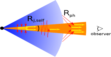
Figure 1: Geometry of the external inverse-Compton (EIC) process. The material producing the external radiation field (ERF) is in blue and the jet in orange. The observer is on the jet axis. The photospheric radius $R_{ph}$ is where the optical depth of the ERF emitting material $\tau(R)=1$ (Eq. 6). The EIC scattering could happen above and below $R_{ph}$. The self-shielding radius $R_{j,self}$ (Eq. 2) is where the jet becomes transparent in the transverse direction. Usually we have $R_{j,self}\ll R_{ph}$, so in the $R_{j,self}<R<R_{ph}$ region, photons may penetrate the jet transversely multiple times before getting scattered.

3.1 EIC emission from above the photosphere

If the observed blackbody luminosity is $L_{BB}$, the ERF flux at the photosphere is

$$F(R_{ph})=\frac{L_{BB}}{4\pi R_{ph}^{2}}$$ (8)

Since $\tau=1$, the ERF at $R_{ph}$ is not far from being isotropic. At radii $R>R_{ph}$, the ERF flux drops as $R^{-2}$ and photons are moving increasingly parallel with the jet, so most of the EIC scatterings happen at radius $R\sim R_{ph}$ and the (isotropic) EIC luminosity is

$$\begin{split}L_{EIC}^{(1)}&\simeq\mbox{min}\left(\frac{4}{\theta_{j}^{2}},4\Gamma^{2}\right)\Gamma^{2}\gamma_{e}^{2}F(R_{ph})2\pi R_{ph}^{2}\theta_{j}\mbox{min}\left(\tau_{j,trvs}(R_{ph}),1\right)\\ &\simeq\mbox{min}\left(1,\theta_{j}^{2}\Gamma^{2}\right)\Gamma^{2}\gamma_{e}^{2}\tau_{j,r}(R_{ph})L_{BB}\end{split}$$ (9)

where $\tau_{j,trvs}$ (Eq. 1) and $\tau_{j,r}$ (Eq. 3) are the optical depth of the jet in the transverse and radial direction. In the second line of Eq.(9), we have used $\tau_{j,trvs}(R_{ph})<1$, because, for parameter space relavant to this work, the condition $\tau_{j,trvs}<1$ is always well satisfied. From Eq.(9), we can see that the EIC process above the photosphere boosts the ERF’s luminosity by a factor of $\Gamma^{2}\gamma_{e}^{2}\tau_{j,r}(R_{ph})\sim 10\gamma_{e}^{2}$.

3.2 EIC emission from below the photosphere

Below the photosphere, the radiation energy in the ERF emitting material has a gradient in the direction where the optical depth $\tau$ drops, so radiation diffuses outwards at a flux (Castor, 2004)

$$F_{dif}(R<R_{ph})\simeq\frac{U(R)c}{3\tau(R)}$$ (10)

where $U(R)$ is the radiation energy density in the ERF emitting material at radius $R$ and $c$ is speed of light. As mentioned above, there is a purely scattering layer between the photosphere and thermalization radius. If the ERF emitting material is expanding, below the radius where photons are advected by electrons (advection radius $R_{adv}$, see section 4.1) or the thermalization radius $R_{th}$, the radiation temperature is controlled by adiabatic expansion (assuming radiation pressure dominates)

$$U\propto T^{4}\propto\rho^{4/3},\ R<\mathrm{max}(R_{th},R_{adv})$$ (11)

In the radius range $\mathrm{max}(R_{th},R_{adv})<R<R_{ph}$, since Comptonization is not efficient enough to change photons’ energy, the diffusive flux follows the inverse square law from energy conservation

$$\frac{Uc}{3\tau}=F(R_{ph})\left(\frac{R}{R_{ph}}\right)^{-2},\ \mathrm{max}(R_{th},R_{adv})<R<R_{ph}$$ (12)

From Eq.(6), (11) and (12), the radial distribution of radiation energy $U(R)$ can be solved, once we know the density profile $\rho(R)$. This is done in 4.1 (Fig. 6) under the assumption that the ERF emitting material is a super-Eddington wind with $\rho\propto R^{-2}$. A similar discussion is given in the context of a wind from ultra luminous X-ray source M101 X-1 by Shen et al. (2015). Below, we take $U(R)$ — the radiation energy density in the ERF emitting material at polar angle $\theta\gg\theta_{j}$ — as known and consider the energy density in the jet funnel.

Due to the removal of photons by jet scattering, the energy density in the funnel will be smaller than in the surrounding material far from the funnel. However, since the jet is narrow, when the optical depth of the jet in the transverse direction $\tau_{j,trvs}$ is small enough, the radiation field in the funnel will not feel the existence of the jet, i.e. it will isotropize and reach energy density $U(R)$. We define an “isotropization radius” $R_{iso}$ where the removal of photons by the jet is balanced by the flux entering the jet funnel $F_{dif}(R)$, i.e.

$$\tau_{j,trvs}Uc=\frac{Uc}{3\tau}\mbox{, or }\tau_{j,trvs}\tau=1/3$$ (13)

In the range $R_{j,self}<R<R_{iso}$, the radiation energy density in the funnel $U_{fnl}(R)$ is smaller than $U(R)$ and is roughly given by

$$\tau_{j,trvs}U_{fnl}c\simeq Uc/3\tau$$ (14)

In the range $R_{iso}<R<R_{ph}$, the radiation energy density in the funnel equals to $U(R)$. Physically, photons cross the funnel back and forth in the transverse direction $1/\tau_{j,trvs}$ times before getting scattered by electrons in the jet, and when $1/\tau_{j,trvs}\sim\tau$, the radiation field can no longer distinguish between the funnel and the region far from the funnel and hence will isotropize. Fig. (2) roughly shows the changing of radiation energy density $U(R)$ with polar angle $\theta$ at different radii $R$.

Figure 2: A sketch for the radiation energy density in the jet funnel $U_{fnl}(R)$ as a function of polar angle $\theta$ at different radii R. Above the “isotropization radius” $R_{iso}$ (defined by Eq. 13), the removal of photons by the jet is balanced by the supplying diffusive flux from the surrounding material, so the radiation energy density at the funnel $U_{fnl}(R)$ reaches the same as in the surrounding material $U(R)$. Below the “self-shielding radius” $R_{j,self}$ (defined by Eq. 2), the jet is optically thick in the transverse direction, so the radiation energy density at the funnel center is approximately zero. In between the two characteristic radii $R_{j,self}<R<R_{iso}$, the radiation energy density in the funnel can be estimated by Eq.(14) as $U_{fnl}\simeq U/(3\tau\tau_{j,trvs})$.

The order of $R_{th}$, $R_{adv}$ and $R_{iso}$ depends on the density profile $\rho(R)$, jet Lorentz factor $\Gamma$ and jet kinetic power $L_{j}$. In the case of a wind density profile $\rho\propto R^{-2}$ in the TDE context, we typically have $R_{th}\lesssim R_{adv}\sim R_{iso}$ (see section 4.1). The EIC luminosity below the photosphere is mostly produced at radius $R\sim R_{iso}$ and we have

$$\begin{split}L_{EIC}^{(2)}&\simeq\mathrm{min}\left(\frac{4}{\theta_{j}^{2}},4\Gamma^{2}\right)\Gamma^{2}\gamma_{e}^{2}F_{dif}(R_{iso})2\pi R_{iso}^{2}\theta_{j}\\ &=\mathrm{min}\left(1,\theta_{j}^{2}\Gamma^{2}\right)\frac{2\Gamma^{2}\gamma_{e}^{2}}{\theta_{j}}L_{BB}\ \mathrm{min}\left[1,\left(\frac{R_{iso}}{R_{adv}}\right)^{1/3}\right]\end{split}$$ (15)

where we have normalized the diffusive flux at $R_{iso}$ to the total luminosity $L_{BB}$ by $F_{dif}(R_{iso})4\pi R_{iso}^{2}=L_{BB}\ \mathrm{min}\left[1,\left(R_{iso}/R_{adv}\right)^{1/3}\right]$. The EIC scattered photons’ peak energy is $\Gamma^{2}\gamma_{e}^{2}2.82kT\mbox{ max}[1,(R_{iso}/R_{adv})^{-2/3}]$. Eq.(15) means that the EIC process below the photosphere boosts the ERF’s luminosity by a factor of $2\Gamma^{2}\gamma_{e}^{2}/\theta_{j}\sim(100-1000)\gamma_{e}^{2}$.

3.3 Corrections for mildly relativistic wind

If the ERF comes from a super-Eddington wind launched from the disk, the wind velocity $\beta_{w}=v_{w}/c$ could be mildly relativistic. In this subsection, we show that relativistic effects make the EIC scattered photons’ energy and EIC luminosities (Eq. 9 and 15) smaller. Depending on $\beta_{w}$, the corrections could be significant. Quantities in the wind comoving frame are denoted by a prime (^′) and those in the lab frame are unprimed.

If the wind Lorentz factor is $\Gamma_{w}=(1-\beta_{w}^{2})^{-1/2}$, the relative Lorentz factor between the jet and wind is $\Gamma_{rel}=\Gamma\Gamma_{w}(1-\beta\beta_{w})\simeq\Gamma\Gamma_{w}(1-\beta_{w})$. For example, if $\Gamma=10$, $\beta_{w}=0.3$ $(0.8)$ gives $\Gamma_{rel}=7.3$ $(3.4)$. After EIC scattering, external photons’ energy is only boosted by a factor of $\Gamma_{rel}^{2}\gamma_{e}^{2}$, which could be much smaller than $\Gamma^{2}\gamma_{e}^{2}$.

If the observed blackbody luminosity and temperature are $L_{BB}$ and $T$, the radiation energy density at the wind photosphere $R_{ph}$ in the wind comoving frame is

$$U^{\prime}(R_{ph})=\frac{L_{BB}}{4\pi R_{ph}^{2}c\Gamma_{w}^{2}}$$ (16)

The wind photospheric radius is different from the non-relativistic case of Eq.(6) by a factor $\Gamma_{w}^{2}$ and is given by

$$\tau_{w}(R)=\kappa_{s}\rho_{w}(R)R/\Gamma_{w}^{2}=1$$ (17)

where the rest mass density $\rho_{w}$ is related to the (rest) mass loss rate by mass conservation

$$4\pi R^{2}\rho_{w}(R)v_{w}=\dot{M}_{w}$$ (18)

Therefore, the EIC luminosity from above the photosphere is

$$\begin{split}L_{EIC}^{(1)}&\simeq\mathrm{min}(1,\theta_{j}^{2}\Gamma^{2})\Gamma_{rel}^{2}\gamma_{e}^{2}\tau_{j,r}(R_{ph})4\pi R_{ph}^{2}U^{\prime}(R_{ph})c\\ &=\mathrm{min}(1,\theta_{j}^{2}\Gamma^{2})\Gamma_{rel}^{2}\gamma_{e}^{2}\tau_{j,r}(R_{ph})L_{BB}/\Gamma_{w}^{2}\end{split}$$ (19)

The EIC luminosity from below the photosphere is mostly produced at the isotropization radius $R_{iso}$ and can be estimated as

$$\begin{split}L_{EIC}^{(2)}&\simeq\mathrm{min}\left(\frac{4}{\theta_{j}^{2}},4\Gamma^{2}\right)\Gamma_{rel}^{2}\gamma_{e}^{2}F_{dif}^{\prime}(R_{iso})2\pi R_{iso}^{2}\theta_{j}\\ &=\mathrm{min}\left(1,\theta_{j}^{2}\Gamma^{2}\right)\frac{2\Gamma_{rel}^{2}\gamma_{e}^{2}}{\theta_{j}}\frac{L_{BB}}{f(\Gamma_{w})}\mathrm{min}\left[1,\left(\frac{R_{iso}}{R_{adv}}\right)^{1/3}\right]\end{split}$$ (20)

Here, the normalization from the diffusive flux $F_{dif}^{\prime}(R_{iso})=U^{\prime}(R_{iso})c/3\tau_{w}(R_{iso})$ to $L_{BB}$ is different from the non-relativistic case used in Eq. (15) by a factor of

$$f(\Gamma_{w})=\Gamma_{w}^{2}(1-\beta_{w}/3)(1+\beta_{w})^{3}$$ (21)

which will be derived in section 4.1. The EIC scattered photons’ peak energy is

$$h\nu_{EIC}=\begin{cases}&\Gamma_{rel}^{2}\gamma_{e}^{2}2.82kT\mbox{, above the photosphere}\\ &\Gamma_{rel}^{2}\gamma_{e}^{2}2.82kT\mathrm{max}\left[1,\left(\frac{R_{iso}}{R_{adv}}\right)^{-2/3}\right]\mbox{, below\ldots}\end{cases}$$ (22)

4 Applications to Sw J2058+05

Similar to the more widely studied event Sw J1644+57, Sw J2058+05 has a rich set of data, in terms of multiwavelength (radio, near-IR, optical, UV, X-ray, $\gamma$-ray) and time coverage (a few to $\sim 200$ days, in the host galaxy rest frame). In this section, we use the data published by Cenko et al. (2012); Pasham et al. (2015) and test if the X-rays from Sw J2058+05 are consistent with the EIC emission from the jet. We focus on Sw J2058+05 because it suffers from a small amount of host galaxy dust extinction and reddening ($A_{V}\lesssim 0.5{\mbox{ }}mag$, while Sw J1644+57 has $A_{V}\sim 5{\mbox{ }}mag$). All quantities (time, frequencies and luminosities) are measured in the host galaxy rest frame at redshift $z=1.185$ (Cenko et al., 2012).

The X-ray lightcurve and spectrum of Sw J2058+05 are similar to Sw J1644+57. The main X-ray properties are as follows: (1) The isotropic luminosity stays $\gtrsim 10^{47}{\mbox{ }}erg{\mbox{ }}s^{-1}$ for $\sim 20{\mbox{ }}d$ and then decline as $\sim t^{-5/3}$ until a sudden drop (by a factor $>160$) at $\sim 200{\mbox{ }}d$. (2) Rapid variability ($\lesssim 500{\mbox{ }}s$) is detected before the drop off, suggesting the X-ray emitting region is at radius $R\sim 10^{15}(\delta t/500{\mbox{ }}s)(\Gamma/10)^{2}{\mbox{ }}cm$. (3) The spectra could be fit by an absorbed powerlaw, with early time ($25-86{\mbox{ }}d$, from Swift/XRT) spectral index $\alpha\sim 0.5$ ($\nu L_{\nu}\propto\nu^{\alpha}$) and late time ($100-200{\mbox{ }}d$) $\alpha\sim 0.2-0.3$. We note that the early time index $\alpha\sim 0.5$ comes from combining all the XRT PC-mode data within $25-86{\mbox{ }}d$, and hence should be taken with caution. We use $\alpha=0.3$ as a typical spectral index in the following.

Figure 3: The early time optical-UV spectra of Sw J2058+05. They are consistent with blackbody. The blue dashed line represents a blackbody spectrum of temperature $T=6\times 10^{4}{\mbox{ }}K$, normalized by $\nu L_{\nu}(10^{15}{\mbox{ }}Hz)=1.3\times 10^{44}{\mbox{ }}erg{\mbox{ }}s^{-1}$. Since the data points only cover the Rayleigh-Jeans tail, the adopted temperature is a lower limit of the true blackbody temperature. All quantities (time, frequencies and luminosities) are measured in the host galaxy rest frame.

The reported optical-UV magnitudes are not corrected for dust extinction. We correct the reddening from the Milky Way (in the direction of this event), using $E(B-V)=0.095{\mbox{ }}mag$ (Cenko et al., 2012, and refs therein). The extinction $A_{b}$ in any band $b$ is calculated by using the tabulated $A_{b}/E(B-V)$ value (at $R_{V}=3.1$) from Schlafly & Finkbeiner (2011). The host galaxy is at redshift $z=1.185$, so the luminosity distance is $2.54\times 10^{28}{\mbox{ }}cm$, if a standard $\Lambda$CDM cosmology is assumed with $H_{0}=71{\mbox{ }}km{\mbox{ }}s^{-1}{\mbox{ }}Mpc^{-1}$, $\Omega_{m}=0.27$, and $\Omega_{\Lambda}=0.73$. We refer to the time of discovery as 00:00:00 on MJD = 55698, following Cenko et al. (2012). The rest-frame time is estimated as $(\mbox{time}-55698)/(1+z)$. We use the effective wavelengths $\lambda_{eff}$ of different filters and the rest-frame frequencies are calculated by $\nu=(1+z)c/\lambda_{eff}$.

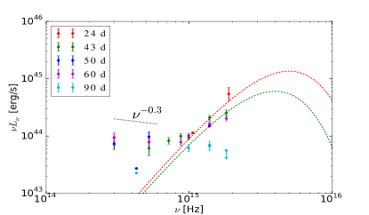
Figure 4: The optical-UV spectra of Sw J2058+05 from $24{\mbox{ }}d$ to $90{\mbox{ }}d$. Apart from the blackbody spectrum, a powerlaw component shows up on the low frequency end. The dashed lines are blackbodies with parameters {$T=6\times 10^{4}{\mbox{ }}K$, $\nu L_{\nu}(10^{15}{\mbox{ }}Hz)=9\times 10^{43}{\mbox{ }}erg{\mbox{ }}s^{-1}$} (red) and {$T=5\times 10^{4}{\mbox{ }}K$, $\nu L_{\nu}(10^{15}{\mbox{ }}Hz)=7\times 10^{43}{\mbox{ }}erg{\mbox{ }}s^{-1}$} (green). Since the data points only cover the Rayleigh-Jeans tail, the adopted temperatures are lower limits. The black dotted line is a representative powerlaw $\nu L_{\nu}\propto\nu^{-0.3}$ (not a fit to the data). Considering the large errorbars and uncertainties from host galaxy reddening, a powerlaw of index $\alpha\sim-0.3$ to $\sim 0.5$ ($\nu L_{\nu}\propto\nu^{\alpha}$) could fit the data. We note that the two data points at $4.3\times 10^{14}{\mbox{ }}Hz$ (from HST/F160W, see Table 2 of Pasham et al. (2015)) seem not consistent with the powerlaw, which could be due to the under estimation of errorbars. However, the blackbody component is not affected. All quantities (time, frequencies and luminosities) are measured in the host galaxy rest frame.

The optical-UV spectra at different time are shown in Fig.(3, 4, 5). The spectrum is purely a blackbody at early time $t\simeq 6-11{\mbox{ }}d$, then a powerlaw component shows up on the low frequency end at $t\simeq 20-60{\mbox{ }}d$, and when $t\gtrsim 100{\mbox{ }}d$, the powerlaw component dominates and the blackbody component becomes invisible. For our purpose, we focus on the blackbody component hereafter (see section 5 for a discussion about the powerlaw component).

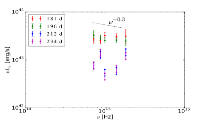
Figure 5: The optical-UV spectra of Sw J2058+05 from $181{\mbox{ }}d$ to $234{\mbox{ }}d$. There is no visible blackbody component, so we can get an upper limit $\nu L_{\nu}(2\times 10^{15}{\mbox{ }}Hz)<2\times 10^{43}\ erg\ s^{-1}$. Considering the large errorbars and uncertainties from host galaxy reddening, a powerlaw of index $\alpha\sim-0.3$ to $\sim 0.5$ ($\nu L_{\nu}\propto\nu^{\alpha}$) could fit the data. The black dotted line is a representative powerlaw $\nu L_{\nu}\propto\nu^{-0.3}$ (not a fit to the data). All quantities (time, frequencies and luminosities) are measured in the host galaxy rest frame.

A blackbody spectrum can be described by two parameters, the bolometric luminosity $L_{BB}$ and the temperature $T$, as follows

$$L_{\nu}=\frac{15hL_{BB}}{\pi^{4}kT}\frac{(h\nu/kT)^{3}}{exp(h\nu/kT)-1}$$ (23)

where $h$ is the Planck constant and $k$ is the Boltzmann constant. Unfortunately, optical-UV observations only cover the Rayleigh-Jeans tail, which is insufficient to fully describe a blackbody spectrum. From Fig.(3) and (4), we can get two pieces of information: (i) a lower limit on the temperature

$$T\geq 6\xi\times 10^{4}{\mbox{ }}K$$ (24)

where $\xi=1$, $1$, $0.8$ when $t=(6-11)$, $24$, $(43-60){\mbox{ }}d$, respectively; (ii) the normalization

$$\nu L_{\nu}(10^{15}{\mbox{ }}Hz)=\chi\times 10^{44}{\mbox{ }}erg{\mbox{ }}s^{-1}$$ (25)

where $\chi=1.3$, $0.9$, $0.7$ when $t=(6-11)$, $24$, $(43-60){\mbox{ }}d$, respectively. Making use of Eq.(23), we can rewrite Eq.(25) as

$$\begin{split}L_{BB}=&6.5\times 10^{44}\chi\left(\frac{T}{4.8\times 10^{4}{\mbox{ }}K}\right)^{4}\\ &\left[exp(4.8\times 10^{4}{\mbox{ }}K/T)-1\right]{\mbox{ }}erg{\mbox{ }}s^{-1}\end{split}$$ (26)

where $T$ is the blackbody temperature (constrained by Eq. 24). Hereafter, we use the approximation $x^{4}[exp(1/x)-1]\simeq 1.4x^{3}$, which is accurate to $\leq 20\%$ when $x\in(1,5)$. Eq.(24) and (26) are all the information we can get from the observed spectra.

In Fig.(5), there’s no visible blackbody component from $181{\mbox{ }}d$ to $234{\mbox{ }}d$, so we get an upper limit $\nu L_{\nu}(2\times 10^{15}{\mbox{ }}Hz)<2\times 10^{43}erg/s$. The jet might have been turned off at this time, because the X-ray sharp drop occurs at $t\sim 200{\mbox{ }}d$.

We note that the host galaxy may contribute a small amount of reddening similar to the Milky Way, which will make the spectra slightly steeper, but the conclusions on the blackbody component (Eq. 24 and 26) are only mildly affected. These uncertainties could be taken into account by the two dimensionless parameters $\xi$ and $\chi$.

In the following two subsections, we first show that the blackbody component can be produced by a super-Eddington wind. Next, we use the observed blackbody component as the ERF and test if the X-ray lightcurve and spectrum are consistent with the EIC emission from above or below the photosphere. Constraints on the jet parameters from the two cases are summarized in Table (1). Note that, since the EIC model in section 3 is under the assumption of the jet being ultra-relativistic ($\Gamma\gg 1$), if the constraints lead to $\Gamma\lesssim 2$, the model is inconsistent with the data.

4.1 Wind Model

The high X-ray luminosity of Sw J2058+05 implies that the accretion stays super-Eddington for a few months. Super-Eddington disks are known to be accompanied by strong winds. For instance, Poutanen et al. (2007) show that strong winds combined with the X-rays from the disk around super-Eddington accreting stellar-mass BHs are in good agreement of the observational data from ultra luminous X-ray sources. The super-Eddington wind could be launched by radiation pressure (e.g. Shakura & Sunyaev, 1973). Rencent radiation-magnetohydrodynamic (rMHD) simulations by Ohsuga & Mineshige (2011, 2D) and Jiang et al. (2014, 3D) show that the kinetic power of (continuum) radiation driven wind can be much higher than $L_{Edd}$. However, the 3D general relativistic rMHD simulations by McKinney et al. (2014) show that the kinetic power of wind from super-Eddington disks around rapidly spinning BHs remains at the order of $L_{Edd}$. Laor & Davis (2014) proposed that the strength of line driven winds sharply rises when the local temperature of the accretion disks around supper massive BHs reaches $\sim 5\times 10^{4}\ K$. It is also likely that magnetic fields (MFs) play an important role in the wind launching process, since angular momentum is removed from an accretion disk through MFs. For example, Blandford & Payne (1982) proposed that the wind could be driven centrifugally along open MF lines.

Up to now, a systematic study of the role of MFs and (line- and continuum-) opacity is still lacking and the detailed wind launching physics is still not well understood. In the context of TDEs, the fact that the fall-back material is very weakly bound is very different from the initial conditions used in the aforementioned numerical simulations. Since the fall-back material evolves nearly adiabatically, the energy released from the accretion of a fraction of the material on bound orbit could push the rest outwards as a wind.

Hereafter, we use upper case $R$ to denote the true radii (in $cm$) and lower case $r=R/R_{S}$ for the dimensionless radii normalized by the Schwarzschild radius $R_{S}=3\times 10^{11}m_{6}{\mbox{ }}cm$. Also, the true accretion, outflowing (subscript “w”), and fallback (subscript “fb”) rates (in $M_{\odot}{\mbox{ }}yr^{-1}$) are denoted as upper case $\dot{M}$ and the dimensionless rates are normalized by the Eddington accretion rate as $\dot{m}=\dot{M}/\dot{M}_{Edd}$. The Eddington accretion rate is defined as $\dot{M}_{Edd}=10L_{Edd}/c^{2}$, and $L_{Edd}=1.5\times 10^{44}m_{6}{\mbox{ }}erg{\mbox{ }}s^{-1}$, where $m_{6}=M/10^{6}M_{\odot}$ is BH mass in $10^{6}M_{\odot}$ and we have assumed solar metallicity with Thomson scattering opacity $\kappa_{s}=0.34\ cm^{2}\ g^{-1}$.

For a star with mass $M_{*}=m_{*}M_{\odot}$ and radius $R_{*}=r_{*}R_{\odot}$, the (dimensionless) tidal disruption radius is

$$r_{T}=\frac{R_{*}}{R_{S}}\left(\frac{M}{M_{*}}\right)^{1/3}\simeq 23.3m_{6}^{-2/3}m_{*}^{-1/3}r_{*}$$ (27)

The star’s original orbit has pericenter distance $r_{p}<r_{T}$. When the star passes $r_{T}$ for the first time, the tidal force from the BH causes a spread of specific orbital energy across the star (Stone et al., 2013)

$$\Delta\epsilon=\frac{GM}{R_{T}}\frac{R_{*}}{R_{T}}$$ (28)

Bound materials have specific orbital energies $-\Delta\epsilon<\epsilon<0$ and the corresponding Keplerian orbital periods $P$ are given by

$$\epsilon=-\frac{1}{2}\left(\frac{2\pi GM}{P}\right)^{2/3}$$ (29)

Therefore, if circularization is efficient enough (within a few orbital periods), the fall back rate is

$$\dot{M}_{fb}=\frac{dM_{*}}{dP}=\frac{dM_{*}}{d\epsilon}\frac{d\epsilon}{dP}=\frac{(2\pi GM)^{2/3}}{3}\frac{dM_{*}}{d\epsilon}P^{-5/3}$$ (30)

which means that a flat distribution of mass per orbital energy gives the mass fall-back rate $\dot{M}_{fb}\propto(t/t_{o})^{-5/3}$. The leading edge of the fall-back material has the shortest period

$$t_{o}=41m_{6}^{1/2}m_{*}^{-1}r_{*}^{3/2}{\mbox{ }}d$$ (31)

Therefore, the normalized fall-back rate profile is

$$\dot{m}_{fb}=1.12\times 10^{2}m_{6}^{-3/2}m_{*}^{2}r_{*}^{-3/2}(t/t_{o})^{-5/3}$$ (32)

Following Strubbe & Quataert (2009), we assume a fraction $f_{out}\in(0.1,1)$ of the fall-back gas is gone with the wind, and hence the wind mass loss rate is $\dot{m}_{w}\sim 10-100$ at early time ($\lesssim 20{\mbox{ }}d$) and $\dot{m}_{w}\propto t^{-5/3}$ later on (if $f_{out}$ stays constant). Note that, in the absence of the wind, the jet might be draged to a halt due to the IC scattering of radiation from the disk as follows. From the conservation of angular momentum, the disk size is $2r_{p}\sim r_{T}\sim 10^{13}\ cm$, which is larger than the self-shielding radius $R_{j.self}$ (Eq. 2). Therefore, at $R=10^{13}\ cm$, disk photons penetrate the jet funnel in the transverse direction and hence the inverse-Compton power of each electron in the jet is $P_{IC}\simeq L_{disk}/(4\pi R^{2})\sigma_{T}\Gamma^{2}\gamma_{e}^{2}$. The ratio of EIC drag timescale, $t_{IC}=\Gamma m_{p}c^{2}/P_{IC}$ (assuming electrons and protons are coupled), and the dynamical timescale, $t_{dy}=R/2c$, is

$$\frac{t_{EIC}}{t_{dy}}=1.7\frac{R_{13}}{L_{disk,45}\Gamma_{1}\gamma_{e}^{2}}$$ (33)

As we show in this paper, an optically thick mildly relativistic wind alleviates this IC drag problem and links the observed optical-UV to the X-ray emission in a self-consistent way.

We assume that the wind is launched from radius $r_{o}=R_{o}/R_{S}$ at a speed $\beta_{w}=v_{w}/c$. Due to inadequate understanding of the wind launching physics, the radius $r_{o}$ is uncertain and hence taken as a free parameter in this work. The rMHD simulations mentioned at the beginning of this subsection show that $r_{o}\sim$ a few.

At the wind launching radius $r_{o}$, we assume that radiation energy and kinetic energy are in equipartition:

$$4\pi R_{o}^{2}\Gamma_{w}^{2}U^{\prime}(R_{o})v_{w}=(\Gamma_{w}-1)\dot{M}_{w}c^{2}$$ (34)

The radiation temperature at the base of the wind $T_{o}^{\prime}$ is related to the radiation energy density by $U^{\prime}(r_{o})=a(T_{o}^{\prime})^{4}$ ($a$ being the radiation density constant), so from Eq.(34), we have

$$T_{o}^{\prime}\simeq 4.9\times 10^{6}\left(\frac{\Gamma_{w}-1}{\Gamma_{w}\beta_{w}}\right)^{1/4}r_{o}^{-1/2}\dot{m}_{w,2}^{1/4}m_{6}^{-1/4}{\mbox{ }}K$$ (35)

Combining Eq. (17) and (18), we obtain the photospheric radius of the wind

$$r_{ph}\simeq\frac{5.0\times 10^{2}\dot{m}_{w,2}}{\Gamma_{w}^{2}\beta_{w}}$$ (36)

Below $r_{ph}$, photons escape by diffusion or advection, and the radius where diffusion time equals to the dynamical time (i.e. $\tau_{w}=c/v_{w}$) is called the “advection radius”

$$r_{adv}\simeq\frac{5.0\times 10^{2}\dot{m}_{w,2}}{\Gamma_{w}^{2}}$$ (37)

At smaller radii $r<r_{adv}$, the wind evolves adiabatically, so the radiation pressure, which dominates over gas pressure ($nkT$), decreases with density as $P=aT^{4}/3\propto\rho^{4/3}$. Under the assumption of a steady wind with constant velocity and spherical symmetry, the density profile is $\rho\propto r^{-2}$, so the radiation temperature (in the comoving frame) evolves as

$$T^{\prime}(r)=T_{o}^{\prime}(r/r_{o})^{-2/3}\mathrm{\ if\ r_{o}<r<r_{adv}}$$ (38)

Here, at a temperature $\gtrsim 10^{5}\ K$, the thermalization radius $r_{th}$ (defined by $\tau^{*}(r_{th})=1$ according to Eq. 7) is related to the photospheric radius by $r_{ph}/r_{th}=(\kappa_{s}/\kappa_{a})^{-1/2}\gtrsim 10$. Since $r_{ph}/r_{adv}=c/v_{w}\lesssim 10$, we usually have $r_{th}\lesssim r_{adv}$. In the range $r_{adv}<r<r_{ph}$, photons only interact with baryons by electron scattering (or Comptonization), which is not efficient enough to change photons’ energy significantly. Therefore, the radiation temperature stays constant as

$$T^{\prime}(r)=T^{\prime}_{adv}=T_{o}^{\prime}(r_{adv}/r_{o})^{-2/3}\mathrm{\ if\ r_{adv}<r<r_{ph}}$$ (39)

Combining Eq.(35), (37) and (39), we find the radiation temperature at the advection radius $T_{adv}^{\prime}$ (in the wind comoving frame). The blackbody temperature to be observed is $T_{w}\simeq\Gamma_{w}T_{adv}^{\prime}$ and is given by

$$T_{w}\simeq 7.8\times 10^{4}\Gamma_{w}^{11/6}\left(\frac{\Gamma_{w}-1}{\beta_{w}}\right)^{1/4}r_{o}^{1/6}m_{w,2}^{-5/12}m_{6}^{-1/4}\mathrm{\ K}$$ (40)

In the range $r_{adv}<r<r_{ph}$, photons escape by diffusion and the diffusive flux follows the inverse square law $F_{dif}^{\prime}=U^{\prime}c/3\tau_{w}\propto r^{-2}$ (since radiation energy is conserved), so we have

$$U^{\prime}(r)=U^{\prime}(r_{adv})(r/r_{adv})^{-3}\mathrm{\ if\ r_{adv}<r<r_{ph}}$$ (41)

The evolution of radiation energy density and temperature with radius in the wind model is shown in Fig.(6).

Figure 6: A sketch for the evolution of radiation energy density $U(R)$ and temperature $T(R)$ with radius $R$. Below the “advection radius” $R_{adv}$ (defined by Eq. 37), the energy density is controlled by adiabatic expansion. Above $R_{adv}$, the energy density decreases with $R$ because of diffusion. Since Comptonization is not efficient enough to change photons’ energy, the radiation temperature stays constant at $R>R_{adv}$.

Next, we Doppler-boost the radiation field from the wind comoving frame to the lab frame to calculate the luminosity seen by the observer. The specific intensity at $r_{ph}$ in the wind comoving frame is

$$\begin{split}I^{\prime}_{\nu^{\prime}}(r_{ph})&=I^{\prime}_{\nu^{\prime}}(r_{adv})\left(\frac{r_{ph}}{r_{adv}}\right)^{-3}\\ &=\beta_{w}^{3}\frac{2h(\nu^{\prime})^{3}}{c^{2}}\frac{1}{\mathrm{e}^{h\nu^{\prime}/kT_{adv}^{\prime}}-1}\end{split}$$ (42)

After Lorentz transformation $I_{\nu}=I^{\prime}_{\nu^{\prime}}(\nu/\nu^{\prime})^{3}$, the specific intensity in the lab frame is still a blackbody and the only difference is that the temperature is a function of the emission latitude angle $\theta$, i.e.

$$I_{\nu}(r_{ph},\theta)=\beta_{w}^{3}\frac{2h\nu^{3}}{c^{2}}\frac{1}{\mathrm{e}^{h\nu/k\tilde{T}(\theta)}-1}$$ (43)

where $\tilde{T}(\theta)=T_{adv}^{\prime}/[\Gamma_{w}(1-\beta_{w}\cos\theta)]$. Note that the difference between relativistic and non-relativistic solutions is the latitude dependence of $\tilde{T}(\theta)$, and the flux ratio is a function of wind Lorentz factor

$$\begin{split}f(\Gamma_{w})&=\frac{\int_{0}^{1}\mu d\mu\int d\nu I_{\nu}(\mu)}{\int_{0}^{1}\mu d\mu\int d\nu^{\prime}I^{\prime}_{\nu^{\prime}}}=\frac{\int_{0}^{1}\mu[\Gamma_{w}(1-\beta_{w}\mu)]^{-4}d\mu}{\int_{0}^{1}\mu d\mu}\\ &=\Gamma_{w}^{2}(1-\beta_{w}/3)(1+\beta_{w})^{3}\end{split}$$ (44)

where $\mu=\cos\theta$ has been used. Note that $f(\Gamma_{w})\rightarrow 16\Gamma_{w}^{2}/3$ in the ultra-relativistic limit and $f(\Gamma_{w})\rightarrow 1$ in the non-relativistic limit. The isotropic equivalent luminosity for an observer at infinity is

$$\begin{split}L_{w}&=4\pi\int_{0}^{1}2\pi R_{ph}^{2}\int I_{\nu}(R_{ph},\mu)d\nu\mu d\mu\\ &=\pi R_{adv}^{2}a(T_{adv}^{\prime})^{4}\beta_{w}cf(\Gamma_{w})\\ &\simeq 5.9\times 10^{44}\Gamma_{w}^{1/3}(\Gamma_{w}-1)f(\Gamma_{w})r_{o}^{2/3}\dot{m}_{w,2}^{1/3}m_{6}\ erg\ s^{-1}\end{split}$$ (45)

from which, we can see that the wind luminosity can mildly exceed the Eddington luminosity (when $\dot{m}_{w}\gg 1$). Putting the optical-UV constraints from Sw J2058+05 (Eq. 24 and 26) into the wind model (Eq. 40 and 45), we find

$$\begin{split}&m_{6}\dot{m}_{w,2}^{19/21}=2.9\frac{\Gamma_{w}^{38/21}}{[f(\Gamma_{w})]^{4/7}(\Gamma_{w}-1)^{1/7}\beta_{w}^{3/7}}\chi^{4/7}r_{o}^{-2/21}\\ &\dot{m}_{w,2}\leq 0.97\frac{[f(\Gamma_{w})]^{3/4}\Gamma_{w}^{29/4}(\Gamma_{w}-1)^{3/2}}{\beta_{w}^{3/4}}\xi^{-21/4}\chi^{-3/4}r_{o}\end{split}$$ (46)

where $\xi=1$, $1$, $0.8$ and $\chi=1.3$, $0.9$, $0.7$ when $t=(6-11)$, $24$, $(43-60){\mbox{ }}d$, respectively. We note that, due to the strong dependence on the temperature (through $\xi$) and wind velocity $\beta_{w}$, the upper limit of mass loss rate $\dot{m}_{w}$ has large uncertainties and so does the lower limit of BH mass $m$. However, the product $m_{6}\dot{m}_{w,2}\simeq m_{6}\dot{m}_{w,2}^{19/21}$ only depends on $\beta_{w}$, decreasing from $\sim 4$ to 2 when $\beta_{w}\in(0.3,0.99)$. Therefore, the true wind mass loss rate can be estimated by

$$\dot{M}_{w}=2.6m_{6}\dot{m}_{w,2}{\mbox{ }}M_{\odot}{\mbox{ }}yr^{-1}\simeq 5\frac{m_{6}\dot{m}_{w}}{200}{\mbox{ }}M_{\odot}{\mbox{ }}yr^{-1}$$ (47)

Note that the derived mass loss rate $\dot{M}_{w}$ is in the isotropic equivalent sense. The wind is expected to be somewhat beamed along the jet axis (towards the observer), so Eq.(47) is consistent with a typical TDE and the optical-UV blackbody component is consistent with being produced by a super-Eddington wind. Note that the advection radius only depends on the product $m_{6}\dot{m}_{w,2}$ and is hence not affected by the uncertainties on the temperature:

$$R_{adv}=3.0\times 10^{14}\frac{1}{\Gamma_{w}^{2}}\frac{m_{6}\dot{m}_{w}}{200}\ cm$$ (48)

And the photospheric radius $R_{ph}$ is a factor $1/\beta_{w}$ larger.

In section 3.2, we defined the “isotropization radius” $R_{iso}$ by balancing the radiation flux entering the jet funnel through the interface with the wind and the flux removed due to EIC scattering. In the relativistic case, $R_{iso}$ is given by

$$\tau_{j,trvs}^{\prime}(R)\tau_{w}(R)=1/3$$ (49)

where $\tau_{j,trvs}^{\prime}(R)=R\theta_{j}n_{e}\sigma_{T}/2\Gamma_{w}$ is the transverse optical depth of the jet in the wind comoving frame and $\tau_{w}(R)=\kappa_{s}\rho_{w}(R)R/\Gamma_{w}^{2}$ is the optical depth of the wind. Below $R_{iso}$, all the diffusive flux $F_{dif}^{\prime}$ entering the jet funnel is scattered by the jet and contributes to the EIC luminosity. At radii $R_{iso}<R<R_{ph}$, the removal of radiation by EIC scattering is not efficient enough, so the radiation energy density in the funnel reaches the same as in the wind region far away from the funnel. Solving Eq.(49), we get

$$R_{iso}\simeq 7.3\times 10^{13}\frac{1}{\Gamma_{w}^{3/2}\beta_{w}^{1/2}}\left(\frac{L_{j,48}\theta_{j,-1}}{\Gamma_{1}}\right)^{1/2}\left(\frac{m_{6}\dot{m}_{w}}{200}\right)^{1/2}{\mbox{ }}cm$$ (50)

4.2 EIC Model

At radii $R<R_{adv}$, the ERF temperature evolves as $T\propto R^{-2/3}$, so the EIC emission is expected to have a powerlaw spectrum

$$\frac{dL_{EIC}}{d\nu}\propto\frac{dL_{EIC}}{dT}=\frac{dL_{EIC}}{dR}\frac{dR}{dT}\propto R\propto T^{-3/2}$$ (51)

from which we get $\nu L_{\nu}\propto\nu^{-1/2}$. This is too soft compared to the observed X-ray powerlaw $\nu L_{\nu}\propto\nu^{0.3}$. Below, we consider the electrons in the jet having a powerlaw distribution function

$$\frac{dN_{e}}{d\gamma_{e}}\begin{cases}\propto\gamma_{e}^{-p}&\mbox{ if }\gamma_{min}<\gamma_{e}<\gamma_{max}\\ =0&\mbox{ otherwise}\end{cases}$$ (52)

The ERF is assumed to have a blackbody spectrum at temperature $T$ and bolometric luminosity $L_{BB}$, so the scattered photons’ spectrum at frequency $\nu\gg\Gamma_{rel}^{2}\gamma_{min}^{2}kT/h$ will be $\nu L_{\nu}\propto\nu^{(3-p)/2}$. Therefore, the observed X-ray spectrum $\nu L_{\nu}\propto\nu^{0.3}$ can be reproduced by an electron index of $p=2.4$.

Another requirement is that the $\nu^{0.3}$ powerlaw extends wider than the $0.3(1+z)-10(1+z){\mbox{ }}keV$ window. We define two (electrons’) Lorentz factors $\gamma_{1}$ and $\gamma_{2}$ corresponding to the scattered photons’ energies

$$\begin{cases}&h\nu_{EIC}(\gamma_{e}=\gamma_{1})=0.3(1+z){\mbox{ }}keV\\ &h\nu_{EIC}(\gamma_{e}=\gamma_{2})=10(1+z){\mbox{ }}keV\\ &\gamma_{min}\leq\gamma_{1}<\gamma_{2}\leq\gamma_{max}\end{cases}$$ (53)

where $2.82kT$ is the blackbody peak energy and $h\nu_{EIC}$ is given by Eq.(22). We focus on the XRT band, because the possible extension in the BAT band (up to $\sim 150(1+z){\mbox{ }}keV$) could be explained by simply extending $\gamma_{max}$ to larger values (but $\gamma_{max}$ is finite so that the EIC luminosity doesn’t diverge).

As pointed out in section 3, the EIC emission could come from above or below the photosphere. The only difference is that the EIC luminosity from below the photosphere is larger by a factor of $2\Gamma_{w}^{2}/[\theta_{j}\tau_{j,r}(R_{ph})f(\Gamma_{w})]\sim 10$ (see Eq. 19 and 20). In the following two subsections, we consider the two possibilities and try to match the expected EIC luminosities in the $0.3(1+z)-10(1+z){\mbox{ }}keV$ window with the observation $L_{X}=10^{47}L_{X,47}{\mbox{ }}erg{\mbox{ }}s^{-1}$.

4.2.1 EIC emission from above the photosphere

In this subsection, we consider the EIC emission from above the photosphere. We convolve Eq.(19), where electrons are assumed to have a single Lorentz factor $\gamma_{e}$, with the Lorentz factor distribution described by Eq.(52). Then we match the EIC luminosity in the $0.3(1+z)-10(1+z){\mbox{ }}keV$ window with observations

$$\begin{split}L_{X}&\simeq\mbox{min}(1,\theta_{j}^{2}\Gamma^{2})\Gamma_{rel}^{2}\gamma_{min}^{2}\tau_{j,r}(R_{ph})L_{BB}\\ &\cdot\frac{p-1}{3-p}\left(\frac{\gamma_{1}}{\gamma_{min}}\right)^{3-p}\left[\left(\frac{\gamma_{2}}{\gamma_{1}}\right)^{3-p}-1\right]\\ &\simeq 10^{47}L_{X,47}{\mbox{ }}erg{\mbox{ }}s^{-1}\end{split}$$ (54)

Combining the X-ray constraints (Eq. 53 and 54) with optical-UV constraints (Eq. 24 and 26), we get

$$\begin{cases}&T/K\simeq\frac{1.0\times 10^{5}\Gamma_{w}^{0.74}}{\left(\Gamma_{rel}\gamma_{min}\right)^{0.52}}\left[\frac{L_{X,47}}{\mathrm{min}(1,\theta_{j}\Gamma^{2})\chi\tau_{j,r}(R_{ph})}\right]^{0.37}\\ &T/K\leq 2.7\times 10^{6}\left(\Gamma_{rel}\gamma_{min}\right)^{-2}\\ &T/K\geq 6\xi\times 10^{4}\end{cases}$$ (55)

Then, we eliminate the parameter $T$ and put the constraints on the Lorentz factors

$$\begin{cases}&\Gamma\gamma_{min}\left[\mbox{min}(1,\theta_{j}^{2}\Gamma^{2})\right]^{-0.25}\leq\frac{9.1}{\Gamma_{w}^{1.5}(1-\beta_{w})}\left(\frac{L_{X,47}}{\chi\tau_{j,r}(R_{ph})}\right)^{-0.25}\\ &\Gamma\gamma_{min}\left[\mbox{min}(1,\theta_{j}^{2}\Gamma^{2})\right]^{0.71}\leq\frac{2.7\Gamma_{w}^{0.43}}{1-\beta_{w}}\left(\frac{L_{X,47}}{\chi\tau_{j,r}(R_{ph})}\right)^{0.71}\xi^{-1.9}\end{cases}$$ (56)

The uncertainty lies on the parameter $\tau_{j,r}(R_{ph})$ (the optical depth of the jet in the radial direction at the ERF’s photosphere $R_{ph}$). Combining Eq.(3) and (36), we have

$$\tau_{j,r}(R_{ph})=0.39\Gamma_{w}^{2}\beta_{w}\frac{L_{j,48}}{\Gamma_{1}}\left(\frac{m_{6}\dot{m}_{w}}{200}\right)^{-1}$$ (57)

4.2.2 EIC emission from below the photosphere

In this subsection, we consider the EIC emission from below the photosphere. Similar to the treatment in section 4.2.1, we match the EIC luminosity in the $0.3(1+z)-10(1+z){\mbox{ }}keV$ window with observations

$$\begin{split}L_{X}&\simeq\mathrm{min}(1,\theta_{j}^{2}\Gamma^{2})\frac{2\Gamma_{rel}^{2}\gamma_{1}^{2}}{\theta_{j}}\frac{L_{BB}}{f(\Gamma_{w})}\mathrm{min}\left[1,\left(\frac{R_{iso}}{R_{adv}}\right)^{1/3}\right]\\ &\cdot\frac{p-1}{3-p}\left(\frac{\gamma_{1}}{\gamma_{min}}\right)^{3-p}\left[\left(\frac{\gamma_{2}}{\gamma_{1}}\right)^{3-p}-1\right]\\ &\simeq 10^{47}L_{X,47}{\mbox{ }}erg{\mbox{ }}s^{-1}\end{split}$$ (58)

Combining the X-ray constraints (Eq. 53 and 58) with optical-UV constraints (Eq. 24 and 26), we get

$$\begin{cases}&T/K\simeq\frac{7.8\times 10^{4}}{(\Gamma_{rel}\gamma_{min})^{0.52}}\left[\frac{L_{X,47}\theta_{j}f(\Gamma_{w})}{\chi\mathrm{min}(1,\theta_{j}^{2}\Gamma^{2})\mathrm{min}\left[1,\left(R_{iso}/R_{adv}\right)^{0.53}\right]}\right]^{0.37}\\ &T/K\leq 2.7\times 10^{6}(\Gamma_{rel}\gamma_{min})^{-2}\mathrm{min}\left[1,\left(\frac{R_{iso}}{R_{adv}}\right)^{2/3}\right]\\ &T/K\geq 6\xi\times 10^{4}\end{cases}$$ (59)

We eliminate the parameter $T$ and put the constraints on the Lorentz factors

$$\begin{cases}&\Gamma\gamma_{min}\left[\frac{\theta_{j}}{\mathrm{min}(1,\theta_{j}^{2}\Gamma^{2})}\right]^{0.25}\leq\frac{10.9\left(\chi/L_{X,47}\right)^{0.25}\mathrm{min}\left[1,\left(R_{iso}/R_{adv}\right)^{0.58}\right]}{\Gamma_{w}(1-\beta_{w})[f(\Gamma_{w})]^{0.25}}\\ &\Gamma\gamma_{min}\left[\frac{\theta_{j}}{\mathrm{min}(1,\theta_{j}^{2}\Gamma^{2})}\right]^{-0.71}\leq\frac{1.68[f(\Gamma_{w})]^{0.71}\left(L_{X,47}/\chi\right)^{0.71}}{\Gamma_{w}(1-\beta_{w})\xi^{1.9}\mathrm{min}\left[1,\left(R_{iso}/R_{adv}\right)^{0.38}\right]}\end{cases}$$ (60)

The ratio of the isotropization radius $R_{iso}$ to the advection radius $R_{adv}$ can be calculated from Eq.(48) and (50)

$$\frac{R_{iso}}{R_{adv}}\simeq 0.24\left(\frac{\Gamma_{w}}{\beta_{w}}\right)^{1/2}\left(\frac{L_{j,48}\theta_{j,-1}}{\Gamma_{1}}\right)^{1/2}\left(\frac{m_{6}\dot{m}_{w}}{200}\right)^{-1/2}$$ (61)

which means $R_{iso}\lesssim R_{adv}$.

4.2.3 Results

Table 1: Summary of the constraints on the jet parameters from the EIC models above and below the photosphere. The three observables $\xi$ (blackbody temperature, Eq. 24), $\chi$ (normalization, Eq. 25), $L_{X,47}$ (X-ray luminosity in the $0.3-10\ keV$ window) are obtained by fitting the data by hand and have uncertainties $\lesssim 30\%$, so the constraints are accurate to within a factor of $\sim 2$. Due to various uncertainties such as host galaxy dust extinction and X-ray absorbed powerlaw fitting, it’s hard to achieve a better accuracy anyway. We consider four different wind velocities $\beta_{w}=v_{w}/c=0.1,\ 0.3,\ 0.6,\ 0.8$ ($\Gamma_{w}=(1-\beta_{w}^{2})^{-1/2}$ is the wind Lorentz factor). We can see that, for a slow wind with $\beta_{w}\lesssim 0.6$, the EIC model from above the photosphere is consistent with observations but that from below the photosphere is inconsistent (marked in red). The physical reason is that the latter over-produces the X-ray luminosities at all or some of the epochs. On the other hand, for a fast wind with $\Gamma_{w}\gtrsim 1.5$, the EIC models from both above and below the photosphere are consistent with observation, with reasonable jet parameters $\Gamma\simeq 5-10$, $\gamma_{min}\sim 1$ and $p=2.4$.

$\beta_{w}$	$0.1\ (\Gamma_{w}-1=$ 5.0e-3)			$0.3\ (\Gamma_{w}-1=$ 4.8e-2)			$0.6\ (\Gamma_{w}=1.25)$			$0.8\ (\Gamma_{w}=1.67)$
$t/d$	$6-11$	24	$43-60$	$6-11$	24	$43-60$	$6-11$	24	$43-60$	$6-11$	24	$43-60$
$\xi$	1	1	0.8	1	1	0.8	1	1	0.8	1	1	0.8
$\chi$	1.3	0.9	0.7	1.3	0.9	0.7	1.3	0.9	0.7	1.3	0.9	0.7
$L_{X,47}$	4.8	0.8	8.5e-2	4.8	0.8	8.5e-2	4.8	0.8	8.5e-2	4.8	0.8	8.5e-2
EIC model above the photosphere, from Eq.(56)
$\Gamma^{5/4}\gamma_{min}\leq$	5.0	4.8	4.7	10.4	10.0	9.8	21.7	20.9	20.4	37.1	35.7	34.7
$\Gamma^{2/7}\gamma_{min}\leq$	22.8	25.5	42.3	6.2	7.0	11.6	3.4	3.8	6.3	3.5	3.9	6.5
EIC model below the photosphere, from Eq.(60)
$\Gamma^{4/3}\gamma_{min}\leq$	14.0	14.7	15.8	15.1	15.8	17.0	18.3	19.2	20.6	22.9	23.9	25.7
$\Gamma^{4/3}\gamma_{min}\leq$	2.0	1.0	0.56	3.7	1.8	1.0	9.4	4.6	2.5	23.8	11.6	6.4

Eq.(56) and (60) are the general constraints on the EIC emission models from above and below the photosphere. However, too many unknown parameters are involved, including $\Gamma$, $\gamma_{min}$, $\theta_{j}$, $\Gamma_{w}$, $\tau_{j,r}(R_{ph})$, and $R_{iso}/R_{adv}$. To express the constraints in a more clear way, we relax some generalities and make two additional assumptions

$$\begin{cases}&L_{j,48}=L_{X,47}\\ &\theta_{j}=\Gamma^{-1}\end{cases}$$ (62)

We have to be cautious not to over-interpret the results, because the two assumptions in Eq.(62) are not derived from first principles. The wind mass loss rate in Eq.(46) can be safely simplified by dropping the $r_{o}^{-2/21}$ term and ignoring the difference between $\dot{m}_{w,2}^{19/21}$ and $\dot{m}_{w,2}$.

At three different epochs ($t=6-11,24$ and $43-60$ d), we put the observables $\xi$ (blackbody temperature, Eq. 24), $\chi$ (normalization, Eq. 25), $L_{X,47}$ (X-ray luminosity in the $0.3-10\ keV$ window) into Eq.(56) and (60), and obtain the constraints on the two Lorentz factors $\Gamma$ and $\gamma_{min}$, as summarized in Table 1. From the variability time $\Gamma\simeq 6(R/10^{15}cm)^{1/2}(\delta t/500s)^{-1/2}$ and radio beaming ($\Gamma\geq 2.1$ Cenko et al., 2012) arguments, the jet must be relativistic. If the product $\Gamma\gamma_{min}$ is restricted to be $\lesssim 2$, the model is not consistent with observations. We note that the unphysical result $\Gamma\gamma_{min}<1$ appears because we assume the jet is ultra-relativistic ($\Gamma\gg 1$) and it simply means the EIC process over-produces the X-ray luminosity.

We find: (1) for a slow wind with $\beta_{w}\lesssim 0.6$, the EIC model from above the photosphere is consistent with observations but that from below the photosphere is inconsistent. The physical reason is that the latter over-produces the X-ray luminosities at all or some of the epochs. (2) For a fast wind with $\Gamma_{w}\gtrsim 1.5$, the EIC models from both above and below the photosphere are consistent with observation, with reasonable jet parameters $\Gamma\simeq 5-10$, $\gamma_{min}\sim 1$ and $p=2.4$.

5 Discussion

In this section, we discuss some potential issues for the EIC scenario proposed in this work.

(i) The X-ray spectral evolution is not considered in the simple model described in this work. For Sw J2058+05, late time ($100-200{\mbox{ }}d$) XMM-Newton observations don’t show significant change in the spectral slope and Swift/XRT observations don’t have enough statistics to constrain the spectral slope. However, for Sw J1644+57, significant spectral changes are found when the flux fluctuates on short ($\sim 1{\mbox{ }}d$) timescale and as the mean flux level evolves on long ($\sim 100{\mbox{ }}d$) timescale (Saxton et al., 2012). Specifically, the spectrum is softer $\nu L_{\nu}\propto\nu^{\sim 0.3}$ at early epochs ($<50{\mbox{ }}d$) and harder $\nu L_{\nu}\propto\nu^{\sim 0.6}$ later on. In the EIC scenario, this hardening could be explained by the following two possibilities: (1) when the accretion rate is smaller at later time, the ERF comes from smaller radii and has a harder spectrum; (2) the electrons’ powerlaw becomes harder at later time. Another issue is whether the X-ray spectrum is always a single powerlaw in the $0.3(1+z)-10(1+z){\mbox{ }}keV$ window. For example, if we repeat the same procedure in section 4.2 in a narrower window, e.g. $1(1+z)-10(1+z){\mbox{ }}keV$, the constraints will be weaker. Swift/XRT observations have too low statistics to pin down this uncertainty, but future wide field-of-view X-ray telescopes will find more jetted TDEs (Donnarumma & Rossi, 2015), and with simultaneous optical-UV coverage, the EIC scenario could be tested to a higher accuracy.

(ii) Another issue is whether the electrons can maintain a powerlaw distribution. The magnetization of the jet $\sigma$ is defined as the ratio of magnetic energy over baryons’ kinetic energy. The strength of magnetic field in the jet comoving frame is

$$B^{\prime}\simeq 8.2\times 10^{2}\frac{[L_{j,48}\mbox{min}(1,\sigma)]^{1/2}}{\Gamma_{1}R_{15}}\ G$$ (63)

The synchrotron cooling time can be estimated as $t_{syn}^{\prime}=\gamma_{e}m_{e}c^{2}/P_{syn}^{\prime}$, where $P_{syn}^{\prime}$ is the synchrotron power. Therefore, the ratio of synchrotron cooling time over dynamical time is

$$\frac{t_{syn}^{\prime}}{t_{dy}^{\prime}}\simeq 0.70\frac{1}{\gamma_{e}}\frac{\Gamma_{1}^{3}R_{15}}{L_{j,48}\mbox{min}(1,\sigma)}$$ (64)

Apart from synchrotron cooling, electrons also suffer from inverse-Compton (IC) cooling by scattering X-ray photons, which have a comoving energy density $U_{x}^{\prime}=L_{X}/(4\pi R^{2}c\Gamma^{2})$. The IC cooling time can be estimated as $t_{IC}^{\prime}=\gamma_{e}m_{e}c^{2}/P_{IC}^{\prime}$, where $P_{IC}^{\prime}$ is the IC power. Therefore, the ratio of IC cooling time over dynamical time is

$$\frac{t_{IC}^{\prime}}{t_{dy}^{\prime}}\simeq 7.0\frac{1}{\gamma_{e}}\frac{\Gamma_{1}^{3}R_{15}}{L_{X,47}}$$ (65)

At $t\simeq 6-11\ d$, we have $L_{X,47}\simeq 5$, so nearly all electrons are in the fast cooling regime (due to either synchrotron or IC cooling). Here, we have used the X-ray radiation field as a conservative estimate of the IC cooling time and the optical-UV photons cause even faster IC cooling. We note that, in the EIC model since $\gamma_{min}\sim 1$, electrons only share a very small fraction of the total jet energy at radius $R\sim 10^{14}-10^{15}\ cm$. Magnetic reconnection or some non-Coulomb interactions between protons and electrons may keep reheating the electrons and maintain the powerlaw distribution.

(iii) Better blackbody temperature measurements or constraints are crucial. The constraints from the two models (Eq. 56 and 60) are both sensitive to the blackbody temperature (through the parameter $\xi$). For Sw J1644+57, high dust extinction prevents us from measuring the temperature accurately. However, up to now, the (small number) statistics show that one out of the two jetted TDEs has low dust extinction, so better temperature measurements in the future might be promising. For Sw J2058+05, due to various uncertainties such as photometric measurements, host galaxy reddening, X-ray powerlaw fitting and crudeness of our model, the constraints on $\Gamma$, $\gamma_{min}$ in Table 1 are accurate to a factor of $\sim 2$.

(iv) As shown in Fig.(4) and (5), a powerlaw component shows up in near-IR at $t\simeq 40{\mbox{ }}d$ and dominates when $t\gtrsim 100{\mbox{ }}d$. The radio data (Cenko et al., 2012) is consistent with optically thin synchrotron emission $F_{\nu}\propto\nu^{1/3}$, so the near-IR powerlaw may be due to external shocks. However, as pointed out by Pasham et al. (2015), the sharp drop in the optical-UV lightcurves between $181$ and $212{\mbox{ }}d$ (and possibly coincident with X-rays) is not consistent with the expectations from the forward shock. A possible explanation could be the reverse shock. Due to possible fast cooling, the emission from the reverse shock may track the jet kinetic power and match the observed $t^{\sim-5/3}$ lightcurve. More radio data is needed to constrain the reverse shock parameters.

(v) We note the possibility that the ERF has a powerlaw instead of blackbody spectrum as assumed in the model in this work. A powerlaw spectrum may come from a hot corona above the disk or shocks. For example, Kawashima et al. (2012) show that Comptonization of disk photons by the thermal electrons at the reflected shock (due to centrifugal barrier) adds a powerlaw extension plus Wien cut-off to the disk SEDs at high frequencies. This mechanism alone can not explain the X-rays in Sw J2058+05, because the temperature of the shock-heated electrons can not reach $1-10\ keV$ (a rough estimate can be obtained from Eq. 35, if the outflowing rate $\dot{m}_{w}$ is replaced by accretion rate $\dot{m}$). The energy budget of the reflected shock is also too small to account for the high X-ray luminosity. However, the Comptonized powerlaw spectrum could act as the ERF for the EIC process in the jet. If the ERF has $\nu L_{\nu}\propto\nu^{0.3}$, electrons in the jet do not need to be accelerated in order to maintain a powerlaw distribution. A self-consistent modeling of the EIC scattering of powerlaw ERF should be done in the future.

(vi) We also note that even if the observed X-rays are from some other processes (e.g. synchrotron emission after magnetic dissipations), the EIC emission has typical luminosity of $10^{45-48}{\mbox{ }}erg{\mbox{ }}s^{-1}$ and could be detected by the current generation of X-ray telescopes up to high redshift $z\sim 1$. When the other processes are less efficient, the EIC component could stand out and dominate. Future wide field-of-view X-ray telescopes, such as eROSITA (Merloni et al., 2012), Einstein Probe, LOFT (Feroci et al., 2012), will be able to find a large number of jetted TDEs and the EIC scenario could be tested. Donnarumma & Rossi (2015) use Sw J1644+57 as a prototype and estimate the detection rates to be $0.1-10{\mbox{ }}yr^{-1}$ for eROSITA (up to redshift $z_{max}\simeq 0.4$) and $1-10^{2}{\mbox{ }}yr^{-1}$ for Einstein Probe and LOFT ($z_{max}\simeq 1$). The rates depend on the jet beaming angle sensitively, with the upper limits coming from $\theta_{j}=1/2$ ($\Gamma=2$) and the lower limit from $\theta_{j}=1/20$ ($\Gamma=20$).

(vii) Lastly, we discuss the Compton drag on the jet from the EIC process. Constraints on jet parameters can be obtained by requiring the EIC luminosity (either from Eq. 19 or 20) to be smaller than the kinetic power of the jet

$$L_{EIC}\leq L_{j}$$ (66)

For simplicity, we assume $\theta_{j}=1/\Gamma$ and $L_{BB}=10^{45}{\mbox{ }}erg{\mbox{ }}s^{-1}$. The EIC luminosity from above the photosphere $L_{EIC}^{(1)}$ (Eq. 19) depends on $\tau_{j,r}(R_{ph})$, which is given by

$$\tau_{j,r}(R_{ph})=0.35\frac{L_{j,48}}{R_{ph,14.5}\Gamma_{1}\mathrm{max}(1,\sigma)}$$ (67)

where $R_{ph,14.5}=R_{ph}/3\times 10^{14}\ cm$ and $\sigma$ is the jet magnetization. Combining Eq.(19), (66) and (67), we obtain

$$\Gamma\gamma_{e}^{2}\leq\frac{2.8\times 10^{2}}{(1-\beta_{w})^{2}}R_{ph,14.5}\mathrm{max}(1,\sigma)$$ (68)

For a typical TDE jet bulk Lorentz factor $\Gamma\sim 10$, the Compton drag argument in Eq.(68) requires $\gamma_{e}\lesssim 10(1-\beta_{w})^{-1}\mathrm{max}(1,\sigma^{1/2})$ at radii $R\sim 10^{14}-10^{15}\ cm$.

The EIC luminosity from below the photosphere $L_{EIC}^{(2)}$ is given by Eq.(20) and we obtain from the Compton drag argument

$$\begin{split}\Gamma\gamma_{e}^{2/3}&\leq 7.9L_{j,48}^{1/3}\frac{(1-\beta_{w}/3)^{1/3}(1+\beta_{w})}{(1-\beta_{w})^{2/3}}\\ &\cdot\mathrm{min}[1,(R_{iso}/R_{adv})^{-1/9}]\mathrm{,\ if\ }\sigma\lesssim 10^{3}\end{split}$$ (69)

which depends very weakly on $\sigma$ through $R_{iso}/R_{adv}\propto\sigma^{-1/2}$. Note that Eq.(69) is only valid when $\sigma\lesssim 10^{3}$, because otherwise we have $R_{iso}\lesssim$ a few $R_{S}$ (Schwarzschild radius) and the expression of EIC luminosity in Eq.(20) breaks down. When $\sigma\gtrsim 10^{3}$, the Compton drag argument can be expressed as the condition that the EIC cooling time of individual electrons should be longer than the dynamical time

$$\frac{t_{EIC}}{t_{dy}}\simeq\frac{\sigma\Gamma m_{p}c^{2}}{\Gamma^{2}\gamma_{e}^{2}Uc\sigma_{T}}\frac{c}{R}\geq 1$$ (70)

where the ERF energy density can be estimated by $U\simeq L_{acc}/(4\pi R^{2}c)$ and $L_{acc}$ is the accretion luminosity of the disk. Also, we have assumed that each electron shares a total energy of $\sigma\Gamma m_{p}c^{2}$ and electrons’ thermal Lorentz factor in the comoving frame is maintained at an arbitrary $\gamma_{e}$. From Eq.(70), we obtain the following constraint on jet and electron Lorentz factors

$$\Gamma\gamma_{e}^{2}\leq 85\sigma_{3}\frac{R_{12}}{L_{acc,46}}\mbox{, if }\sigma\gtrsim 10^{3}$$ (71)

Any model trying to explain the X-ray data needs to take the constraints from the Compton drag into account. For example, if the X-rays are produced by synchrotron emission, then at least a small fraction of jet electrons must be accelerated to Lorentz factor $\gamma_{e}\gtrsim 10^{3}(B^{\prime}/10^{3}\ G)^{-1/2}$. The Compton drag arguments (Eq. 68, 69 and 71) impose upper limits on the hot electron fraction at the corresponding radii.

6 Summary

In jetted TDEs, the relativistic jet is expected to intercept a strong external radiation field (ERF) and electrons in the jet will inverse-Compton scatter the ERF. In this work, we calculate the external inverse-Compton (EIC) emission from the jet.

In the case of Sw J2058+05, there is a blackbody component in the optical-UV spectrum. We show that the blackbody component is consistent with being produced by a super-Eddington wind. Using the observed blackbody component as the ERF, we test if the X-ray luminosity and spectrum are consistent with the EIC emission. First, to match the powerlaw spectrum $\nu L_{\nu}\propto\nu^{\sim 0.3}$, electrons need to have a powerlaw distribution $dN_{e}/d\gamma_{e}\propto\gamma_{e}^{-p}$ $(\gamma_{min}<\gamma_{e}<\gamma_{max})$ with $p\simeq 2.4$. Then, we try to match the expected EIC luminosity in the $0.3-10\ keV$ window with the observation. We find that for a slow wind of speed $\beta_{w}=v_{w}/c\lesssim 0.6$, the EIC emission from above the photosphere is consistent with observations but that from below the photosphere over-produces the X-ray luminosity. On the other hand, if the wind is mildly relativistic with $\Gamma_{w}\gtrsim 1.5$, the EIC emission from both above and below the photosphere is consistent with observations with jet parameters $\Gamma\simeq 5-10$ and $\gamma_{min}\sim 1$.

We show that even if the observed X-rays are from some other processes (e.g. magnetic dissipations, see Kumar & Crumley (2015) and Crumley et al. (2015)), the EIC emission proposed in this work has typical luminosity of $10^{45}-10^{48}{\mbox{ }}erg{\mbox{ }}s^{-1}$ and could be detected by current generation of X-ray telescopes up to high redshift $z\sim 1$. Future wide field-of-view X-ray surveys, such as eROSITA (Merloni et al., 2012), Einstein Probe, LOFT (Feroci et al., 2012) will be able to find a large number of jetted TDEs and the EIC model could be tested.

We also show that the ERF may impose significant Compton drag on the jet. The requirement that the Compton drag doesn’t bring the jet to a halt constrains the bulk Lorentz factor $\Gamma$ and electrons’ (thermal) Lorentz factor $\gamma_{e}$ in the jet comoving frame. For example, if the jet opening angle $\theta_{j}=\Gamma^{-1}$ and the thermal ERF has luminosity $10^{45}\ erg\ s^{-1}$, we find $\Gamma\gamma_{e}^{2}\lesssim 3\times 10^{2}(1-\beta_{w})^{-2}\mbox{max}(1,\sigma^{1/2})$ at $R\sim 10^{14}-10^{15}\ cm$ (the photospheric radius of the ERF emitting material), where $\sigma$ is the magnetization of the jet. Studying the EIC emission may help us to understand the composition of the jet and constrain the radius where the jet energy is converted to radiation.

7 acknowledgments

We acknowledge helpful discussions with R.-F. Shen, S. Markov and R. Santana. We thank the anonymous referee for a thorough review of the paper, which helped to significantly improve the text. This research was funded by a graduate fellowship (“Named Continuing Fellowship”) at the University of Texas at Austin.

References

- Arcavi et al. (2014) Arcavi, I., Gal-Yam, A., Sullivan, M., et al. 2014, ApJ, 793, 38
- Badnell et al. (2005) Badnell, N. R., Bautista, M. A., Butler, K., et al. 2005, MNRAS, 360, 458
- Barniol Duran & Piran (2013) Barniol Duran, R., & Piran, T. 2013, ApJ, 770, 146
- Blandford & Payne (1982) Blandford, R. D., & Payne, D. G. 1982, MNRAS, 199, 883
- Blandford & Znajek (1977) Blandford, R. D., & Znajek, R. L. 1977, MNRAS, 179, 433
- Bloom et al. (2011) Bloom, J. S., Giannios, D., Metzger, B. D., et al. 2011, Science, 333, 203
- Burrows et al. (2011) Burrows, D. N., Kennea, J. A., Ghisellini, G., et al. 2011, Nature, 476, 421
- Castor (2004) Castor, J. I. 2004, Radiation Hydrodynamics, by John I. Castor, pp. 368. ISBN 0521833094. Cambridge, UK: Cambridge University Press, November 2004.,
- Cenko et al. (2012) Cenko, S. B., Krimm, H. A., Horesh, A., et al. 2012, ApJ, 753, 77
- Chornock et al. (2014) Chornock, R., Berger, E., Gezari, S., et al. 2014, ApJ, 780, 44
- Crumley et al. (2015) Crumley, P., Lu, W., Santana, R., Hernández, R. A., Markoff, S., Kumar, P. 2015, submitted to MNRAS
- Donley et al. (2002) Donley, J. L., Brandt, W. N., Eracleous, M., & Boller, T. 2002, AJ, 124, 1308
- Donnarumma & Rossi (2015) Donnarumma, I., & Rossi, E. M. 2015, ApJ, 803, 36
- Feroci et al. (2012) Feroci, M., Stella, L., van der Klis, M., et al. 2012, Experimental Astronomy, 34, 415
- Gezari et al. (2012) Gezari, S., Chornock, R., Rest, A., et al. 2012, Nature, 485, 217
- Gezari et al. (2009) Gezari, S., Heckman, T., Cenko, S. B., et al. 2009, ApJ, 698, 1367
- Holoien et al. (2014) Holoien, T. W.-S., Prieto, J. L., Bersier, D., et al. 2014, MNRAS, 445, 3263
- Jiang et al. (2014) Jiang, Y.-F., Stone, J. M., & Davis, S. W. 2014, ApJ, 796, 106
- Kalberla et al. (2005) Kalberla, P. M. W., Burton, W. B., Hartmann, D., et al. 2005, A&A, 440, 775
- Kasen & Ramirez-Ruiz (2010) Kasen, D., & Ramirez-Ruiz, E. 2010, ApJ, 714, 155
- Kawashima et al. (2012) Kawashima, T., Ohsuga, K., Mineshige, S., et al. 2012, ApJ, 752, 18
- Komossa et al. (2004) Komossa, S., Halpern, J., Schartel, N., et al. 2004, ApJL, 603, L17
- Kumar & Crumley (2015) Kumar, P., & Crumley, P. 2015, MNRAS, 453, 1820
- Laor & Davis (2014) Laor, A., & Davis, S. W. 2014, MNRAS, 438, 3024
- Levan et al. (2011) Levan, A. J., Tanvir, N. R., Cenko, S. B., et al. 2011, Science, 333, 199
- Liu et al. (2013) Liu, J.-F., Bregman, J. N., Bai, Y., Justham, S., & Crowther, P. 2013, Nature, 503, 500
- Lodato et al. (2009) Lodato, G., King, A. R., & Pringle, J. E. 2009, MNRAS, 392, 332
- Lodato & Rossi (2011) Lodato, G., & Rossi, E. M. 2011, MNRAS, 410, 359
- McKinney et al. (2014) McKinney, J. C., Tchekhovskoy, A., Sadowski, A., & Narayan, R. 2014, MNRAS, 441, 3177
- Merloni et al. (2012) Merloni, A., Predehl, P., Becker, W., et al. 2012, arXiv:1209.3114
- Mészáros & Rees (2000) Mészáros, P., & Rees, M. J. 2000, ApJ, 530, 292
- Mimica et al. (2015) Mimica, P., Giannios, D., Metzger, B. D., & Aloy, M. A. 2015, MNRAS, 450, 2824
- Mukai et al. (2005) Mukai, K., Still, M., Corbet, R. H. D., Kuntz, K. D., & Barnard, R. 2005, ApJ, 634, 1085
- Ohsuga & Mineshige (2011) Ohsuga, K., & Mineshige, S. 2011, ApJ, 736, 2
- Pasham et al. (2015) Pasham, D. R., Cenko, S. B., Levan, A. J., et al. 2015, ApJ, 805, 68
- Piran et al. (2015) Piran, T., Svirski, G., Krolik, J., Cheng, R. M., & Shiokawa, H. 2015, ApJ, 806, 164
- Poutanen et al. (2007) Poutanen, J., Lipunova, G., Fabrika, S., Butkevich, A. G., & Abolmasov, P. 2007, MNRAS, 377, 1187
- Rees (1988) Rees, M. J. 1988, Nature, 333, 523
- Rybicki & Lightman (1979) Rybicki, G. B., & Lightman, A. P. 1979, New York, Wiley-Interscience
- Saxton et al. (2012) Saxton, C. J., Soria, R., Wu, K., & Kuin, N. P. M. 2012, MNRAS, 422, 1625
- Saxton et al. (2012) Saxton, R. D., Read, A. M., Esquej, P., et al. 2012, A&A, 541, AA106
- Schlafly & Finkbeiner (2011) Schlafly, E. F., & Finkbeiner, D. P. 2011, ApJ, 737, 103
- Shakura & Sunyaev (1973) Shakura, N. I., & Sunyaev, R. A. 1973, A&A, 24, 337
- Shen et al. (2015) Shen, R.-F., Barniol Duran, R., Nakar, E., & Piran, T. 2015, MNRAS, 447, L60
- Stone et al. (2013) Stone, N., Sari, R., & Loeb, A. 2013, MNRAS, 435, 1809
- Strubbe & Quataert (2009) Strubbe, L. E., & Quataert, E. 2009, MNRAS, 400, 2070
- Takahashi et al. (2014) Takahashi, T., Mitsuda, K., Kelley, R., et al. 2014, Proc. SPIE, 9144, 914425
- Tchekhovskoy et al. (2011) Tchekhovskoy, A., Narayan, R., & McKinney, J. C. 2011, MNRAS, 418, L79
- van Velzen & Farrar (2014) van Velzen, S., & Farrar, G. R. 2014, ApJ, 792, 53
- Wang & Merritt (2004) Wang, J., & Merritt, D. 2004, ApJ, 600, 149
- Wang et al. (2014) Wang, J.-Z., Lei, W.-H., Wang, D.-X., et al. 2014, ApJ, 788, 32
- Zauderer et al. (2011) Zauderer, B. A., Berger, E., Soderberg, A. M., et al. 2011, Nature, 476, 425
- Zauderer et al. (2013) Zauderer, B. A., Berger, E., Margutti, R., et al. 2013, ApJ, 767, 152