A NUMERICAL MODEL FOR ACCRETION
IN INTERMEDIATE POLARS WITH DIPOLAR
MAGNETIC FIELDS

Abstract

Received April 3, 2015;   in final form April 10, 2015

A three-dimensional numerical model for an accretion process investigation in the magnetosphere of a white dwarf in magnetic cataclysmic variables is developed. The model assumes that the white dwarf has a dipole magnetic field with its symmetry axis inclined to the rotation axis. The model is based on the equations of modified MHD, that describe the mean flow parameters in the wave MHD turbulence. Diffusion of the magnetic field and radiative heating and cooling are taken into account. The suitability of the model is confirmed by modeling the accretion in a typical intermediate polar. The computations show that a magnetosphere forms around the accretor, with the accretion occurring via columns. The accretion columns have a curtain-like shape, and arc-shaped zones of energy release form on the surface of the white dwarf in the magnetic poles area as a result of the matter infall.

DOI: 10.1134/S106377291509005X

1 INTRODUCTION

Studies of accretion processes are the most important and topical problems of modern astrophysics. In many cases, the intrinsic magnetic field of the accretor plays a substantial role in this process. We consider here magnetic cataclysmic variables as investigation objects. These are close binary systems consisting of a low-mass late-type star (donor) and a white dwarf (accretor) Warner1995 , the donor fills its Roche lobe. The pressure gradient at the inner Lagrangian point L₁ is not balanced by gravity, and matter starts to flow into the Roche lobe of the compact object. Two main types of magnetic cataclysmic variables can be distinguished: polars and intermediate polars. In polars the accretorhas a substantial magnetic field ($>10^{6}$ G) and magnetosphere that extends to the inner Lagrangian point L₁ , prevent the formation of an accretion disk. The accretion proceeds along magnetic-field lines onto the magnetic poles of the accretor. In intermediate polars, the magnetic field of the accretor is relatively weak ($10^{4}$–$10^{6}$ G), and an accretion disk can form in the system, whose inner radius is limited of the size of the magnetosphere. The interaction of the disk material and the magnetic field of the accretor leads to the formation of a complex flow structure, that can include accretion columns and belts. The flow structure in intermediate polars also depends strongly on the inclination of the magnetic axis, the magnetic field geometry, and the rotational velocity of the accretor.

The three-dimensional (3D) numerical model of the accretion taking into account the magnetic field of the accretor was for the first time developed in Koldoba2002 . This model made it possible to describe in detail the 3D structure of the flow in the magnetosphere of the gravitating object, where the magnetic field is dominant. The following studies of these authors Romanova2003 ; Romanova2004a ; Romanova2004b presented the results of 3D numerical modeling of plasma accretion onto a gravitating object with a dipole magnetic field whose axis of symmetry is not aligned with the rotational axis of the star. For the first time 3D MHD simulation of disk accretion onto a star with a complex magnetic field geometry was carried out in Long2007 ; Long2008 . More complex magnetic field configurations were considered in Romanova2011 , taking into account the octupolar component. These models were used to study disk accretion onto young T Tauri stars.

In the series of our papers zb2009 ; ZhilkinMM2010 ; zbASR2010 ; zbMFG ; zbSMF ; zbbUFN ; bycam1 (see also the monograph mcbook ), we developed a 3D numerical model for mass transfer in semidetached binary systems taking into account the magnetic field of the accretor. The model assumes that the plasma dynamics are determined by the slow mean flow, against the background of that highspeed MHD waves propagate. A strong external magnetic field acts as an efficient fluid and interacts with the plasma. The model takes into account the inclination of the magnetic axis relative to the rotational axis, the diffusion of the magnetic field, and radiative heating and cooling. This model allowed us for the first time to achieve a selfconsistent description of the MHD flow structure in close binary systems, including such characteristic features as the accretion disk, the magnetosphere of the accretor, accretion columns, etc. However, over our limited computer resources, we focused on studies of the outer regions of the accretion disk, that can be observed using classical astronomy methods. We did not consider the flow structure near the surface of the accretor in detail before. In our present paper, we describe the numerical model that allows detailed study of the flow characteristics in the vicinity of the accretor magnetosphere in the frame of our general approach. This makes it possible, in particular, to study the penetration of plasma into the magnetospheres of white dwarfs and neutron stars in more detail.

The paper is organized in the following way. Section $2$ describes the model, and Section $3$ is the numerical method. The results of the 3D numerical modeling are presented in Section $4$. We discuss the main results of our study in the Conclusion.

2 DESCRIPTION OF THE MODEL

The object of our study is a close binary system with the parameters of the typical intermediate polar Warner1995 . The donor (red dwarf) has a mass of $M_{d}=0.1\leavevmode\nobreak\ M_{\odot}$ and an effective temperature of $4000\leavevmode\nobreak\ \text{K}$. The mass of the white dwarf is $M_{a}=0.8\leavevmode\nobreak\ M_{\odot}$. The orbital period of the system is $P_{\text{orb}}=1.6\leavevmode\nobreak\ hr$, and the component separation is $A=0.7\leavevmode\nobreak\ R_{\odot}$. We assume that the magnetic field of the white dwarf can be correctly described by a dipole field. The surface field of the white dwarf is varied from $8$ to $80\leavevmode\nobreak\ \text{kG}$. The inclination of the magnetic axis to the rotational axis is $30^{\circ}$. To describe the flow structure in our numerical model, we have used a noninertial reference frame corotating with the binary system with angular velocity $\Omega=2\pi/P_{\text{orb}}$ relative to its center of mass. The field strength in this system is described by the Roche potential

$$\Phi=-\frac{GM_{a}}{|{\bf r}-{\bf r}_{a}|}-\frac{GM_{d}}{|{\bf r}-{\bf r}_{d}|}-\frac{1}{2}\left[{\bf\Omega}\times\left({\bf r}-{\bf r}_{c}\right)\right]^{2},$$ (1)

where $G$ is the gravitational constant, ${\bf r}_{a}$ — the radius vector of the center of the accretor, ${\bf r}_{d}$ — the radius vector of the center of the donor, and ${\bf r}_{c}$ — the radius vector of the center of mass of the binary system. We use the Cartesian coordinate system $(x,y,z)$ with the origin coincident with the center of the accretor. The center of the donor is located at $(-A,0,0)$, and the $z$ axis is directed along the axis of the system rotation, ${\bf\Omega}=(0,0,\Omega)$.

The vector of the dipole magnetic field is given by

$${\bf B}_{*}=\frac{3\left(\bm{\mu}\cdot{\bf r}\right){\bf r}}{r^{5}}-\frac{\bm{\mu}}{r^{3}},$$ (2)

where $\bm{\mu}$ is the magnetic moment of the accretor. To reduce the numerical errors, we represent the total magnetic field ${\bf B}$ as a superposition of the intrinsic magnetic field of the accretor ${\bf B}_{*}$ and the field ${\bf b}$ induced by currents in the plasma: ${\bf B}={\bf B}_{*}+{\bf b}$ Tanaka1994 .

In the general case, the rotation of the accretor is asynchronous, and it is characterized in the reference frame selected by the angular velocity ${\bf\Omega}_{a}$. In the case of synchronous rotation, ${\bf\Omega}_{a}=0$. We consider here the case when the rotational axis of the accretor is aligned with the rotation axis of the binary system. Thus, the magnetic field of the accretor is nonstationary:

$${\frac{\partial{{\bf B}_{*}}}{\partial{t}}}=\mathop{\rm rot}\nolimits({\bf v}_{*}\times{\bf B}_{*}),$$ (3)

where ${\bf v}_{*}={\bf\Omega}_{a}\times({\bf r}-{\bf r}_{a})$ is the velocity of the magnetic field lines of the accretor.

The plasma in the vicinity of the magnetospheres of the magnetic white dwarfs in cataclysmic variables is magnetized zbbUFN and moves in the external magnetic field. The intrinsic magnetic field of the plasma ${\bf b}$ is then much weaker than the intrinsic magnetic field of the white dwarf ${\bf B}_{*}$. In this case, the velocity of the plasma can be much lower than the propagation velocity of MHD waves. In regions of strong magnetic fields or low density, the velocity of propagation of Alfvén and magnetosonic waves can be even relativistic. Over the dynamical time scale, such MHD waves have time to cross the accretion stream in the longitudinal and transverse directions many times. Therefore, the plasma dynamics in the stream can be considered in the framework of modified magnetogasdynamics as a sort of mean flow against the background of a wave MHD turbulence. To describe the motion of the plasma in this case we define the rapidly propagating MHD fluctuations and apply a certain averaging procedure over the ensemble of wave pulsations. Such model was developed by us earlier in zbSMF ; zbbUFN .

Strictly speaking, this model is correct only in the presence of a strong external magnetic field, as is the case of polars and in the magnetospheres of intermediate polars. However, the results of calculations zbuAIP2013 have demonstrated that this model is sufficiently universal. With an appropriate choice of parameters (for example, the parameter determining the efficiency of the wave turbulence), this model also well describes the flow structure in the case of weak magnetic fields. Accordingly, we adopted it as the basis for our description of accretion in magnetic cataclysmic variables in the vicinity of the white dwarf magnetosphere.

Taking into account the magnetic field, the flow of matter in a close binary system may be described by the system of equationszbbUFN :

$${\frac{\partial{\rho}}{\partial{t}}}+\nabla\cdot\left(\rho{\bf v}\right)=0,$$ (4)

$${\frac{\partial{{\bf v}}}{\partial{t}}}+\left({\bf v}\cdot\nabla\right){\bf v}=-\frac{\nabla P}{\rho}-\frac{{\bf b}\times\mathop{\rm rot}\nolimits{\bf b}}{4\pi\rho}-\nabla\Phi+2\left({\bf v}\times{\bf\Omega}\right)-\frac{\left({\bf v}-{\bf v}_{*}\right)_{\perp}}{t_{w}},$$ (5)

$${\frac{\partial{{\bf b}}}{\partial{t}}}=\mathop{\rm rot}\nolimits\left[{\bf v}\times{\bf b}+\left({\bf v}-{\bf v}_{*}\right)\times{\bf B}_{*}-\eta\,\mathop{\rm rot}\nolimits{\bf b}\right],$$ (6)

$$\rho T\left[{\frac{\partial{s}}{\partial{t}}}+\left({\bf v}\cdot\nabla\right)s\right]=n^{2}\left(\Gamma-\Lambda\right)+\frac{\eta}{4\pi}\left(\mathop{\rm rot}\nolimits{\bf b}\right)^{2}.$$ (7)

where $\rho$ is the density, ${\bf v}$ — the velocity, $P$ — the pressure, $s$ — the entropy per unit mass, $n=\rho/m_{p}$ — the number density, $m_{p}$ — the proton mass, $\eta$ — the coefficient of magnetic viscosity, and $\Gamma$ and $\Lambda$ — the radiative heating and cooling functions, respectively. The density, entropy and pressure are related by the equation of state of an ideal gas,

$$s=c_{\text{V}}\ln(P/\rho^{\gamma}),$$ (8)

where $c_{\text{V}}$ is the specific heat capacity at constant volume and $\gamma=5/3$ is the adiabatic index. The last term in the equation of motion (5) describes the force of the white dwarf magnetic field acting on the plasma, that influences the plasma velocity perpendicular to the magnetic field lines zbSMF ; zbbUFN . The time scale for the decay of the transverse velocity is

$$t_{w}=\frac{4\pi\rho\eta_{w}}{B^{2}_{*}},$$ (9)

where $\eta_{w}$ — is the coefficient of magnetic viscosity due to wave MHD turbulence.

The numerical model takes into account the effects of diffusion of the magnetic field [in (6) and (7)] caused by magnetic reconnection and the dissipation of currents in turbulent vortices Bisnovatyi-Kogan76 ; zb2009 ; zbbUFN , magnetic buoyancy Campbell97 ; zb2009 ; zbbUFN and wave MHD turbulence zbSMF ; zbbUFN . The coefficient of the wave viscosity is given by

$$\eta_{w}=\alpha_{w}\frac{l_{w}B_{*}}{\sqrt{4\pi\rho}},$$ (10)

where $l_{w}=B_{*}/|\nabla B_{*}|$ is the characteristic spatial scale of the wave pulsations, and $\alpha_{w}$ — a dimensionless factor that is close to unity that determines the efficiency of the wave diffusion. The diffusion of the magnetic field is nonlinear in whole.

3 NUMERICAL METHOD

The system (4)–(7) is quite difficult to solve numerically directly. Therefore, it is convenient to divide it according to physical processes into simpler subsystems. Each subsystem can be solved using specific numerical methods. Let us suppose that we know the distribution of all values in the computational domain at time $t^{n}$. To obtain the values at the next time step, corresponding to the time $t^{n+1}=t^{n}+\Delta t$, we apply an algorithm with five sequential steps, described briefly below.

In the first step, we distinguish the subsystem of equations describing the dynamics of the plasma in its own magnetic field:

$${\frac{\partial{\rho}}{\partial{t}}}+\nabla\cdot\left(\rho{\bf v}\right)=0,$$ (11)

$${\frac{\partial{{\bf v}}}{\partial{t}}}+\left({\bf v}\cdot\nabla\right){\bf v}=-\frac{\nabla P}{\rho}-\frac{{\bf b}\times\mathop{\rm rot}\nolimits{\bf b}}{4\pi\rho},$$ (12)

$${\frac{\partial{{\bf b}}}{\partial{t}}}=\mathop{\rm rot}\nolimits\left({\bf v}\times{\bf b}\right),$$ (13)

$${\frac{\partial{s}}{\partial{t}}}+({\bf v}\cdot\nabla)s=0.$$ (14)

The form of this subsystem coincides with the equations of ideal magnetogasdynamics. This subsystem can be solved numerically using the higher-order Godunov-type difference scheme described below in this section. In the second step, the variations of the gas velocity due to external forces (the Coriolis force and the gradient of the Roche potential) are taken into account:

$${\frac{\partial{{\bf v}}}{\partial{t}}}=2({\bf v}\times{\bf\Omega})-\nabla\Phi.$$ (15)

In this step, the remaining variables are taken to be constant. The Roche potential $\Phi$ is time independent. Therefore, we compute new values for the velocity ${\bf v}$ using the analytic solution of this equation in the interval $t^{n}\leq t\leq t^{n+1}$.

The third step of the algorithm considers the deceleration force during the motion of the plasma across magnetic field lines, as well as the generation of magnetic field due to this motion. The corresponding equations can be written

$$\begin{gathered}{\frac{\partial{{\bf v}_{\perp}}}{\partial{t}}}=-\frac{({\bf v}-{\bf v}_{*})_{\perp}}{t_{w}},\\ {\frac{\partial{{\bf b}}}{\partial{t}}}=\mathop{\rm rot}\nolimits\left[({\bf v}-{\bf v}_{*})_{\perp}\times{\bf B}_{*}\right].\end{gathered}$$ (16)

We compute the new values of the velocity ${\bf v}$ and magnetic field ${\bf b}$ using analytical solutions of these equations in the interval $t^{n}\leq t\leq t^{n+1}$.

In the fourth step of the algorithm, we take into account the effects of the magnetic field diffusion. The corresponding equation is

$${\frac{\partial{{\bf b}}}{\partial{t}}}=-\mathop{\rm rot}\nolimits\left(\eta\mathop{\rm rot}\nolimits{\bf b}\right).$$ (17)

This equation is nonlinear in our model. Therefore, it was solved numerically using an implicit, locally one-dimensional method with a factorisable operator Samarsky1989 ; mcbook .

Finally, the fifth step includes the effects of radiative heating and cooling, as well as heating due to current dissipation. These processes are described by the right hand side of Eq. (7).

Let us describe the method used to solve the hyperbolic subsystem (11)–(14) in more detail. We can rewrite these equations in conservative form in the Cartesian coordinates $x^{1}=x$, $x^{2}=y$, $x^{3}=z$ as follows:

$${\frac{\partial{\cal U}}{\partial{t}}}+{\frac{\partial{{\cal F}_{1}}}{\partial{x^{1}}}}+{\frac{\partial{{\cal F}_{2}}}{\partial{x^{2}}}}+{\frac{\partial{{\cal F}_{3}}}{\partial{x^{3}}}}=0.$$ (18)

Here, ${\cal U}$ and ${\cal F}_{k}$ (where the subscript $k$ runs through the values 1, 2, 3) denote vectors of conservative variables and fluxes, defined by the expressions

$${\cal U}=\left(\begin{matrix}\rho\\ \rho{\bf v}\\ {\bf b}\\ \rho s\end{matrix}\right),\quad{\cal F}_{k}=\left(\begin{matrix}\rho v_{k}\\ \rho{\bf v}{v}_{k}+{\bf n}_{k}\left(P+{\bf b}^{2}/8\pi\right)-{\bf b}b_{k}/4\pi\\ {\bf b}v_{k}-{\bf v}b_{k}\\ \rho sv_{k}\end{matrix}\right),$$ (19)

where ${\bf n}_{k}$ are unit vectors directed along the axes of the Cartesian coordinate system.

We now transform the variables $x^{k}$ in these equations into the new variables $\xi^{k}$ using the transformation of coordinates. In the new curvilinear coordinates $\xi^{k}$, it is convenient to introduce the local basis vectors ${\bf e}_{k}={\partial{\bf r}}/{\partial\xi^{k}}$, directed tangentially to the corresponding coordinate lines. In general, this basis is nonorthogonal and nonnormalized. In addition to these vectors, we can also consider the vectors of the reciprocal (dual) basis ${\bf e}^{1}={\bf e}_{2}\times{\bf e}_{3}$, ${\bf e}^{2}={\bf e}_{3}\times{\bf e}_{1}$ and ${\bf e}^{3}={\bf e}_{1}\times{\bf e}_{2}$, , that are orthogonal to the corresponding coordinate lines. The vectors of the reciprocal basis are also nonorthogonal and nonnormalized in the general case. The Jacobian of the coordinate transformation can be written $Q={\bf e}_{1}\cdot({\bf e}_{2}\times{\bf e}_{3})$.

In the new variables, the system of equations (18) acquires the form

$${\frac{\partial{{\cal U}}}{\partial{t}}}+\frac{1}{Q}{\frac{\partial{{\cal H}_{1}}}{\partial{\xi^{1}}}}+\frac{1}{Q}{\frac{\partial{{\cal H}_{2}}}{\partial{\xi^{2}}}}+\frac{1}{Q}{\frac{\partial{{\cal H}_{3}}}{\partial{\xi^{3}}}}=0,$$ (20)

where the fluxes

$${\cal H}_{k}=\sum\limits_{i=1}^{3}e^{k}_{i}{\cal F}_{i},$$ (21)

and $e^{k}_{1}$, $e^{k}_{2}$ and $e^{k}_{3}$ denote the components of the vectors ${\bf e}^{k}$ of the reciprocal basis in Cartesian coordinates. We obtained a numerical solution of this system of equations using a high-order, Godunov- type difference scheme ZhilkinMM2010 , providing a third- order approximation in the spatial variable in the area of the smooth solution and a first order approximation in time. With appropriate boundary conditions, this difference scheme ensures accurate satisfaction of the conservation laws for the physical quantities in the space of the original variables ($x$, $y$, $z$). The stability of the scheme is provided by the limited time step $\Delta t$ (the Courant–Friedrichs– Lewy condition).

In the computations considered below, we use the spherical coordinates $\xi^{1}=r$, $\xi^{2}=\theta$, $\xi^{3}=\varphi$ as curvilinear coordinates, that are related to the Cartesian coordinates by the expressions

$$x=r\sin\theta\cos\varphi,\quad y=r\sin\theta\sin\varphi,\quad z=r\cos\theta.$$ (22)

The solution was obtained in the computational domain ($0.015A\leq r\leq 0.08A$, $0\leq\theta\leq\pi$, $0\leq\varphi\leq 2\pi$). We use a $N_{r}\times N_{\theta}\times N_{\varphi}=128\times 128\times 256$ grid in the numerical computations.

We use the following boundary and initial conditions. A free inflow condition is specified at the inner boundary, corresponding to the surface of the accretor. We adopt the magnetic field condition ${\bf b}=0$. We neglect additional heating of the matter due to the absorption of radiation from the accretion zones. The fields at the surface of the accretor are taken to be typical for intermediate polars. In such systems, mass transfer leads to the formation of an accretion disk. Therefore, we specify conditions corresponding to the distributions of variables in an accretion disk at the outer boundary of the computational domain. The vertical density distribution is defined using the condition of hydrostatic equilibrium in an isothermal disk with temperature $10000\leavevmode\nobreak\ \text{K}$. We apply the conditions $v_{\varphi}=v_{\text{K}}$ and $v_{r}=-0.1v_{\text{K}}$ for the velocities, where $v_{\text{K}}$ is the velocity of the Keplerian rotation. In the equatorial plane of the disk, we specify the density to be $\rho=10^{-3}\rho(\textrm{L}_{1})$, where $\rho(\textrm{L}_{1})$ is the density at the inner Lagrangian point L₁ corresponding to a mass transfer rate $\dot{M}=10^{-10}\leavevmode\nobreak\ M_{\odot}/\text{yr}$. The initial conditions in the computational domain are following: initial density $\rho=10^{-6}\rho(\textrm{L}_{1})$, initial velocity ${\bf v}=0$, initial temperature $T=10000\leavevmode\nobreak\ \text{K}$, and initial magnetic field ${\bf b}=0$.

We use the 3D parallel code zbbUFN ; ZhilkinMM2010 for the numerical simulation. The computations for all the models were continued until the quasistationary regime begins, it is defined by approximate (up to 1%) constancy of the total mass in the computational domain. The computations were carried out at the computer cluster of the Joint Supercomputer Center of the Russian Academy of Sciences using 512 processors.

4 COMPUTATION RESULTS

Here we present the results of our simulation of the flow structure for magnetic fields at the surface of the accretor of $B_{a}=8\leavevmode\nobreak\ \text{kG}$ (Model 1) and $B_{a}=80\leavevmode\nobreak\ \text{G}$ (Model 2). The inclination of the magnetic axis to the rotational axis ($z$) was $30^{\circ}$ in both cases. Since the radius of the magnetosphere exceeds the radius of the accretor in both models, the accretion has a magnetogasdynamical rather than gas dynamical character.

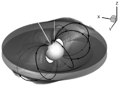
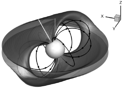
Figure 1: Flow structure (side view) for $B_{a}=8\leavevmode\nobreak\ \text{kG}$ (left) and $B_{a}=80\leavevmode\nobreak\ \text{kG}$ (right). Surfaces of constant logarithm of the density are shown in the shade of gray, the magnetic field lines by lines with arrows, the rotation axis by the thin white solid line, and the magnetic axis by the bold white solid line.

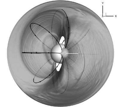
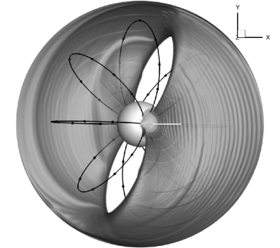
Figure 2: Same as Fig. 1 shown from above.

The 3D structure of the flow is shown in Figs. 1 and 2. The left panels correspond to the Model 1, and the right panels — to the Model 2. The bright sphere corresponds to the accretor and the shade of gray shows isosurfaces of logarithm of the density. The curved lines with arrows indicate the direction of the magnetic field lines. The thin, white solid line is directed along the $z$ axis and corresponds to the rotational axis of the accretor, while the bold, white solid line shows the magnetic axis.

Analysis of these figures shows the formation of a magnetosphere near the surface of the accretor, where the matter moves mainly along magnetic field lines. This results in column accretion, with the matter reaching the surface of the accretor in the vicinity of its magnetic poles. The accretion disk has a nonuniform vertical structure. The disk thickness decreases in places where the accretion columns begin to form. Two cavities (vacuum regions) that are free of matter form between the accretion disk and the accretor; the magnetic field hinders the penetration of matter into these regions, since the field lines pass mainly along the stellar surface close to the magnetic equator. The size of this vacuum region increases with the field strength. Figure 2 shows that these regions are tilted by some angle; this is due to the rotation of the matter in the disk, which causes the accretion column shifts in the direction opposite to the direction of rotation.

Figures 1 and 2 show that, in both cases, the accretion column has a curtain-like, rather than tube- like, shape. The curtain is broader and more dense in the Model 1, and its opening angle is almost equal to $180^{\circ}$. The curtain occupies a much smaller volume in the Model 2, and is narrower and less dense. In both cases, the matter arrives to the surface of the white dwarf in the shape of two arcs, forming hot spots where energy is released.

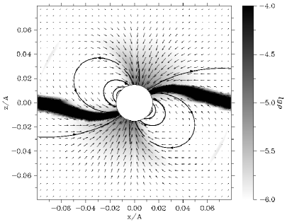
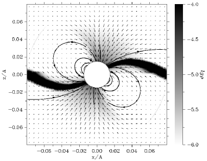
Figure 3: Flow structure in the vertical ($xz$) plane for the Model 1 (left) and Model 2 (right). The distribution of the logarithm of the density is shown in the shade of gray in units of $\rho(\textrm{L}_{1})$) together with the distribution of the velocity (arrows). The lines with arrows correspond to the magnetic field lines.

The flow structure in the vertical ($xz$) plane is shown in Fig. 3. The left diagram corresponds to the Model 1 and the right diagram — to the Model 2. The distribution of the logarithm of the density (in units of $\rho(\textrm{L}_{1})$) is shown in the shade of gray. The arrows show the velocity distribution, and the lines with arrows show magnetic field lines. The flow pattern shown is consistent with what was said above, and all features of the flow structures noted above are clearly visible: the magnetospheric region, accretion columns, and vacuum cavities. The difference in the flow structures for these two models in the $xz$ plane is fairly weak. The difference is manifest more clearly in an analysis of the 3D distributions.

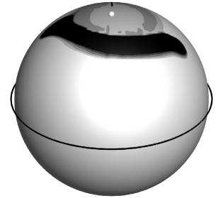
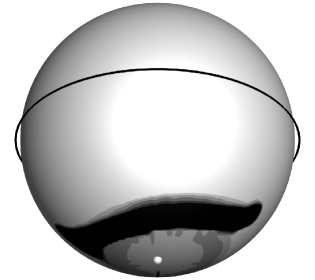
Figure 4: Distribution of the logarithm of the density at the surface of the accretor for $B_{a}=8\leavevmode\nobreak\ \text{kG}$ (left) and $B_{a}=8\leavevmode\nobreak\ \text{kG}$ (right). The black line corresponding to the magnetic equator is shown. The positions of the Northern (top) and Southern (bottom) magnetic poles are shown by the small white circles.

The shape of the hot spots is demonstrated in Fig. 4, that presents the distributions of the logarithm of the density at the stellar surface for the Model 1 (left) and Model 2 (right). The upper diagrams focus on the Northern hemisphere and hot spot, and the lower diagrams on the Southern hemispheres and hot spot. The white circles mark the positions of the Northern and Southern magnetic poles (upper and lower diagrams, respectively). The curved line corresponds to the magnetic equator.

These figures show that the areas of energy release have an arc-like shape (parts of an ellipse), that is clearly due to the effect of gravity. For particles moving along the magnetic field lines, it is energetically more profitable to fall onto the surface of the accretor closer to the equator. Therefore, the highest density is observed in precisely these places. The falling of matter at the opposite end of the circumpolar accretion rings requires a larger expense of energy.

The hot spot is more uniform and occupies a larger area in the Model 1 (weaker magnetic field). This is explained by the dependence of the wave magnetic viscosity and the decay time on the magnetic field strength $\eta_{w}\propto B_{*}$ in Eq. (9) and $t_{w}\propto 1/B_{*}$ and (10) in Eq. (9). As a result, the force from the external magnetic field acting on the plasma (the last term in Eq. (5)) is proportional to the field $B_{*}$. Therefore, the plasma can more easily move across the magnetic field lines in a weaker field (Model 1), and the accretion hot spot spreads over a larger area.

Each spot in the Model 1 occupies about 7% of the stellar surface. The opening angles of the Northern and Southern spots are approximately $170^{\circ}$. In the Model 2 (stronger magnetic field), the spot area is smaller and the density distribution in the spot is more nonuniform. Most of the accretion flow is concentrated toward the center of the spot. In Model 2, the spot occupies about 4% of the stellar surface area, and the opening angle of the spots is about $140^{\circ}$.

5 CONCLUSION

We have developed a three-dimensional numerical model that allows the detail studies of the flow structure near the surface of the accretor in a magnetic close binary system. The model assumes that the intrinsic magnetic field of the accretor is dipole, with the dipole axis inclined to the rotational axis. The model is based on the equations of modified magnetogasdynamics, that describe the mean characteristics of the flow in the frame of the wave MHD turbulence. This approach performed well in our earlier calculations of the flow structure in intermediate polars and polars. The numerical model takes into account diffusion of the magnetic field and radiative heating and cooling processes.

We have presented here the results of 3D numerical simulations of accretion in a typical intermediate polar. The calculations were performed for two intrinsic accretor magnetic fields — 8 kG and 80 kG — and an inclination of the magnetic axis to the rotational axis of $30^{\circ}$. The results show the formation of a magnetosphere close to the accretor, with the accretion occurring through columns. The accretion columns have a curtain-like rather than tubular shape. The flow structure depends substantially on the field strength, although the picture does not change qualitatively for different field strengths. With increasing magnetic field strength, the magnetosphere expands, the vacuum regions become larger, and the opening angles of the curtains decrease. The zones of energy release (hot spots) at the surface of the white dwarf that form in the vicinity of the magnetic poles as a result of the matter inflow and they have the shape of arcs or sections of an ellipse. Increasing the field strength results in an increase in the hot spots area and a decrease in the their opening angles.

This work was supported by the Russian Foundation for Basic Research (projects 14-29-06059, 14-02-00215, 15-02-06365), Basic Research Program P-41 of the Presidium of The Russian Academy of Sciences, by the President of the Russian Federation Grant NSh- 3620.2014.2).

References

- (1) B. Warner, Cataclysmic variable stars (Cambridge: Cambridge Univ. Press, 1995).
- (2) A.V. Koldoba, M.M. Romanova, G.V. Ustyugova, and R.V.E. Lovelace, Astrophys. J. (Letters) 576, L53 (2002).
- (3) M.M. Romanova, G.V. Ustyugova, A.V. Koldoba, J.V. Wick, and R.V.E. Lovelace, Astrophys. J. 595, 1009 (2003).
- (4) M.M. Romanova, G.V. Ustyugova, A.V. Koldoba, J.V. Wick, and R.V.E. Lovelace, Astrophys. J. 610, 920 (2004).
- (5) M.M. Romanova, G.V. Ustyugova, A.V. Koldoba, J.V. Wick, R.V.E. Lovelace, Astrophys. J. (Letters) 616, L151 (2004).
- (6) M. Long, M.M. Romanova, and R.V.E. Lovelace, Monthly Not. Roy. Astron. Soc. 374, 436 (2007).
- (7) M. Long, M.M. Romanova, and R.V.E. Lovelace, Monthly Not. Roy. Astron. Soc. 386, 1274 (2008).
- (8) M.M. Romanova, M. Long, F.K. Lamb, A.K. Kulkarni, and J.-F. Donati, Monthly Not. Roy. Astron. Soc. 411, 915 (2011).
- (9) A. G. Zhilkin and D. V. Bisikalo, Astron. Rep. 53, 436 (2009).
- (10) A. G. Zhilkin, Mat. Model. 22, 110 (2010).
- (11) A.G. Zhilkin and D.V. Bisikalo, Adv. Space Res. 45, 437 (2010).
- (12) A. G. Zhilkin and D. V. Bisikalo, Astron. Rep. 54, 840 (2010).
- (13) A. G. Zhilkin and D. V. Bisikalo, Astron. Rep. 54, 1063 (2010).
- (14) A. G. Zhilkin, D. V. Bisikalo, and A. A. Boyarchuk, Phys. Usp. 55, 115 (2012).
- (15) A. G. Zhilkin, D. V. Bisikalo, and P. A. Mason, Astron. Rep. 56, 257 (2012).
- (16) D. V. Bisikalo, A. G. Zhilkin, and A. A. Boyarchuk, Gas Dynamics of Close Binary Stars (Fizmatlit, Moscow, 2013) [in Russian].
- (17) T. Tanaka, J. Comp. Phys. 111, 381 (1994).
- (18) A.G. Zhilkin, D.V. Bisikalo, and V.A. Ustyugov, AIP Conf. Proc. 1551, 22 (2013).
- (19) G.S. Bisnovatyi-Kogan and A.A. Ruzmaikin, Astrophys. and Space Sci. 42, 401 (1976).
- (20) C. G. Campbell, Magnetohydrodynamics in binary stars (Dorfrecht/Boston/London: Kluwer Acad. Publs, 1997).
- (21) A. A. Samarskii, The Theory of Differential Schemes (Nauka, Moscow, 1989; Marcel Dekker, New York, 2001).