Inverse Inequality Estimates
with
Symbolic Computation

Abstract.

In the convergence analysis of numerical methods for solving partial differential equations (such as finite element methods) one arrives at certain generalized eigenvalue problems, whose maximal eigenvalues need to be estimated as accurately as possible. We apply symbolic computation methods to the situation of square elements and are able to improve the previously known upper bound, given in “$p$- and $hp$-finite element methods” (Schwab, 1998), by a factor of $8$. More precisely, we try to evaluate the corresponding determinant using the holonomic ansatz, which is a powerful tool for dealing with determinants, proposed by Zeilberger in 2007. However, it turns out that this method does not succeed on the problem at hand. As a solution we present a variation of the original holonomic ansatz that is applicable to a larger class of determinants, including the one we are dealing with here. We obtain an explicit closed form for the determinant, whose special form enables us to derive new and tight upper resp. lower bounds on the maximal eigenvalue, as well as its asymptotic behaviour.

1. Introduction

Interdisciplinary collaborations between different areas of mathematics can be hard work because of different terminology and the difficulty of recognizing the applicability of the methods from one field in the other field. In Linz there is an almost-20-year tradition of bringing together researchers from numerical mathematics and symbolic computation [20, 21, 15, 1], which at the beginning faced exactly these kinds of problems. Additionally, there could be the risk that the results are only interesting for one community and not rewarded by the other one. Fortunately, this didn’t happen in our case: in the current work, we use and invent tools at the frontier of symbolic computation to solve a problem that arose at the frontier of numerical analysis research. Hence, this work improves the knowledge and tools for both communities.

Inverse inequalities of the form

(1) $$\left|\left|v_{n}\right|\right|_{X(\Omega)} \leq c_{1}(h,n)\left|\left|v_{n}\right|\right|_{Y(\Omega)}\qquad\text{for all }v_{n}\in V_{n},$$

(2) $$\left|\left|v_{n}\right|\right|_{Z(\partial\Omega)} \leq c_{2}(h,n)\left|\left|v_{n}\right|\right|_{Y(\Omega)}\qquad\text{for all }v_{n}\in V_{n}$$

play an important role in the analysis and design of numerical methods for partial differential equations [4, 22, 2, 6] and in the construction of efficient solvers for the arising linear systems of those methods [10, 23]. Bounds for the constants of the type (1)–(2) have been studied for example in [22, 25, 24, 9, 7], where the asymptotic behaviour with respect to $h$ and $n$ is covered but usually these constants are over estimated. In many numerical methods a precise knowledge of these constants is required, which motivates this work where we use and present tools from symbolic computation to derive precise estimates.

Here $\Omega\subset\mathbb{R}^{d},d\in\mathbb{N}$, is a bounded and open set with sufficiently smooth boundary $\partial\Omega$, describing a finite element with diameter $h>0$ which is used in the numerical method (intervals for $d=1$, often triangles or quadrilaterals for $d=2$, usually tetrahedra or hexahedra for $d=3$, …). Let $V$ be some infinite-dimensional space of functions defined on $\Omega$ such that the solution of the PDE is an element of $V$. With $(V_{n})_{n\in\mathbb{N}}$ we denote a family of finite-dimensional (usually closed) subspaces of $V$ whose dimension depends on $n$; the desired solution of the PDE is approximated by an element of $V_{n}$. Moreover we have some given norms $\left|\left|\cdot\right|\right|_{X(\Omega)}$, $\left|\left|\cdot\right|\right|_{Y(\Omega)}$ and $\left|\left|\cdot\right|\right|_{Z(\partial\Omega)}$ which are induced by certain inner products $\left(\cdot,\cdot\right)_{X(\Omega)}$, $\left(\cdot,\cdot\right)_{Y(\Omega)}$ and $\left(\cdot,\cdot\right)_{Z(\partial\Omega)}$, which are used in the analysis of the numerical methods. In general the constants $c_{1}$ and $c_{2}$ of (1) and (2) depend on the diameter $h$ and on the parameter $n$ reflecting the dimension of the space $V_{n}$. The dependence with respect to the diameter $h$ is obtained by transforming Equations (1) and (2) to a reference domain $\hat{\Omega}\subset\mathbb{R}^{d}$, i.e.

(3) $$\left|\left|\hat{v}_{n}\right|\right|_{X(\hat{\Omega})} \leq\hat{c}_{1}(n)\left|\left|\hat{v}_{n}\right|\right|_{Y(\hat{\Omega})}\qquad\text{for all }\hat{v}_{n}\in\hat{V}_{n},$$

(4) $$\left|\left|\hat{v}_{n}\right|\right|_{Z(\partial\hat{\Omega})} \leq\hat{c}_{2}(n)\left|\left|\hat{v}_{n}\right|\right|_{Y(\hat{\Omega})}\qquad\text{for all }\hat{v}_{n}\in\hat{V}_{n}$$

and applying a scaling argument [22, 25, 2]. The more challenging problem is to find precise estimates for the constants $\hat{c}_{1}$ and $\hat{c}_{2}$ with respect to the parameter $n$. The best possible constants by definition are given by

(5) $$\hat{c}_{1}(n) =\sup_{\hat{v}_{n}\in\hat{V}_{n}}\frac{\left|\left|\hat{v}_{n}\right|\right|_{X(\hat{\Omega})}}{\left|\left|\hat{v}_{n}\right|\right|_{Y(\hat{\Omega})}}=\sqrt{\sup_{\hat{v}_{n}\in\hat{V}_{n}}\frac{\left(\hat{v}_{n},\hat{v}_{n}\right)_{X(\hat{\Omega})}}{\left(\hat{v}_{n},\hat{v}_{n}\right)_{Y(\hat{\Omega})}}},$$

(6) $$\hat{c}_{2}(n) =\sup_{\hat{v}_{n}\in\hat{V}_{n}}\frac{\left|\left|\hat{v}_{n}\right|\right|_{Z(\partial\hat{\Omega})}}{\left|\left|\hat{v}_{n}\right|\right|_{Y(\hat{\Omega})}}=\sqrt{\sup_{\hat{v}_{n}\in\hat{V}_{n}}\frac{\left(\hat{v}_{n},\hat{v}_{n}\right)_{Z(\hat{\partial\Omega})}}{\left(\hat{v}_{n},\hat{v}_{n}\right)_{Y(\hat{\Omega})}}}.$$

Introducing for $\hat{V}_{n}$ the basis functions $(\varphi_{k})_{1\leq k\leq n}$, i.e., $\hat{V}_{n}=\mathrm{span}\{\varphi_{1},\dots,\varphi_{n}\}$, we further obtain

$$\bigl{(}\hat{c}_{1}(n)\bigr{)}^{2}=\sup_{\underline{v}_{n}\in\mathbb{R}^{n}}\frac{\left(K_{n}\underline{v}_{n},\underline{v}_{n}\right)_{\ell^{2}}}{\left(M_{n}\underline{v}_{n},\underline{v}_{n}\right)_{\ell^{2}}}\quad\text{and}\quad\bigl{(}\hat{c}_{2}(n)\bigr{)}^{2}=\sup_{\underline{v}_{n}\in\mathbb{R}^{n}}\frac{\left(L_{n}\underline{v}_{n},\underline{v}_{n}\right)_{\ell^{2}}}{\left(M_{n}\underline{v}_{n},\underline{v}_{n}\right)_{\ell^{2}}},$$

with the symmetric and positive (semi-) definite matrices

$$K_{n}(i,j):=\left(\varphi_{j},\varphi_{i}\right)_{X(\hat{\Omega})},\ M_{n}(i,j):=\left(\varphi_{j},\varphi_{i}\right)_{Y(\hat{\Omega})},\ \text{and}\ L_{n}(i,j):=\left(\varphi_{j},\varphi_{i}\right)_{Z(\hat{\partial\Omega})}$$

for $i,j=1,\ldots,n$. Note that the rows of the matrices are naturally defined via the second argument of the inner product and the columns are given naturally via the first argument of the inner product. Hence, the constants $(\hat{c}_{1})^{2}$ and $(\hat{c}_{2})^{2}$ are given by the largest eigenvalues of the generalized eigenvalue problems

(7) $$K_{n}\underline{x}_{n}=\lambda_{n}M_{n}\underline{x}_{n}\qquad\text{and}\qquad L_{n}\underline{x}_{n}=\mu_{n}M_{n}\underline{x}_{n},$$

i.e.

$$\bigl{(}\hat{c}_{1}(n)\bigr{)}^{2}=\lambda_{n}\qquad\text{and}\qquad\bigl{(}\hat{c}_{2}(n)\bigr{)}^{2}=\mu_{n}.$$

In this work we want to solve the problems (3) and (4), i.e., determine estimates for $\hat{c}_{1}(n)$ and $\hat{c}_{2}(n)$, for the reference domain $\hat{\Omega}=(-1,1)^{2}$ with

$$\left(u,v\right)_{X(\hat{\Omega})} =\int_{\hat{\Omega}}\partial_{x}u(x,y)\partial_{x}v(x,y)\,\mathrm{d}x\,\mathrm{d}y,$$

$$\left(u,v\right)_{Y(\hat{\Omega})} =\int_{\hat{\Omega}}u(x,y)v(x,y)\,\mathrm{d}x\,\mathrm{d}y,$$

for $u,v\in\hat{V}_{n}$, where $\hat{V}_{n}$ is the space of polynomials of degree less than $n$, i.e.

$$\hat{V}_{n}=\left\{x^{i}y^{j}:0\leq i,j<n\right\}.$$

In Section 2 we state the problem in detail and derive its formulation as a generalized eigenvalue problem of the form (7). The difficulty is now to find an accurate estimate for the largest eigenvalues $\lambda_{n}$ and $\mu_{n}$ for general parameter $n\in\mathbb{N}$. Of course one can compute the eigenvalues exactly for a given fixed parameter $n$, which is done for example in [19]. But to derive their exact values or precise estimates for a general parameter $n$ one needs techniques from symbolic computation. In Section 3 we use the HolonomicFunctions package [11, 12] to prove a closed-form representation of the characteristic polynomial of our eigenvalue problem, in the spirit of the holonomic ansatz [27] for evaluating determinants. The holonomic ansatz is a very powerful method (it was the key to the “holy grail of enumerative combinatorics” [14]), and a very flexible one, too [16]. For our purposes here we had to adapt this algorithm, which led to a new variant that is applicable to a larger class of determinants. In Section 4, our representation of the characteristic polynomial is used to derive and prove the estimates from below and above

$$\frac{1}{4}\sqrt{n(n-1)(n+1)(n+2)}\leq\hat{c}_{1}(n)\leq\frac{1}{2\sqrt{2}}\sqrt{n(n-1)(n+1)(n+2)}$$

for the constant $\hat{c}_{1}(n)$ in the inequality

$$\left|\left|\partial_{\hat{x}}\hat{u}_{n}\right|\right|_{L^{2}(\hat{\Omega})}\leq\hat{c}_{1}(n)\left|\left|\hat{u}_{n}\right|\right|_{L^{2}(\hat{\Omega})}\qquad\text{for all }\hat{u}_{n}\in\hat{V}_{n}.$$

In Lemmas 4.5 and 4.8 we give much sharper estimates for $\hat{c}_{1}(n)$; as an application, they allow to tune the parameters of numerical methods precisely. In Section 5 the same representation is used to investigate the asymptotic behaviour of the eigenvalues; on the way we discover some interesting connections to the Taylor expansions of trigonometric functions. As an encore, we deal with the second inequality (4) in Section 6. It turns out that it is considerably simpler and we are able to derive the exact value of $\hat{c}_{2}(n)$.

Throughout the paper, we employ the following notation: $(a)_{n}$ denotes the Pochhammer symbol, also known as rising factorial, defined for all nonnegative integers $n$ by

$$(a)_{n}:=a\cdot(a+1)\cdots(a+n-1)\text{ for }n>0\quad\text{and}\quad(a)_{0}:=1.$$

We use $\lfloor x\rfloor$ for the floor function, and $\lceil x\rceil$ for the ceiling function, i.e., the largest integer below $x$, resp. the smallest integer above $x$. For a polynomial $p$ we refer to the degree of $p$ with respect to the variable $x$ by $\deg_{x}(p)$. By $\delta_{i,j}$ we denote the Kronecker delta symbol, i.e., $\delta_{i,j}=0$ if $i\neq j$ and $\delta_{i,i}=1$. If $A$ is the $n\times n$ matrix $(a_{i,j})_{1\leq i,j\leq n}$, then we use for its determinant the short-hand notation $\det(A)=\det_{1\leq i,j\leq n}(a_{i,j})$. The determinant of the $0\times 0$ matrix is defined to be $1$.

2. The Maximal Eigenvalue Problem

Let the reference domain $\hat{\Omega}\subset\mathbb{R}^{2}$ be defined by $\hat{\Omega}:=(-1,1)^{2}$, the open square of size $2$ centered around the origin. For $n\in\mathbb{N}$ and $k\in\{1,\dots,n^{2}\}$, we define $\chi_{n}(k)$ and $\rho_{n}(k)$ to be the unique integers in $\{0,\dots,n-1\}$ satisfying $k=\chi_{n}(k)\cdot n+\rho_{n}(k)+1$. In other words,

$$\chi_{n}(k):=\Bigl{\lfloor}\frac{k-1}{n}\Bigr{\rfloor}\qquad\text{and}\qquad\rho_{n}(k):=k-1\mathrel{\mathrm{mod}}n.$$

For the rest of this section we fix $n\in\mathbb{N}$ and write shortly $\chi(k)$ and $\rho(k)$. By employing the standard monomial basis $\varphi_{k}:=x^{\rho(k)}t^{\chi(k)}$, we obtain the $n^{2}\times n^{2}$ matrix $M_{n}$ with entries $m_{i,j}$ defined by

(8) $$m_{i,j}:=\int_{\hat{\Omega}}\varphi_{i}\varphi_{j}\,\mathrm{d}x\,\mathrm{d}t\qquad(1\leq i,j\leq n^{2})$$

and the $n^{2}\times n^{2}$ matrix $K_{n}$ with entries

(9) $$k_{i,j}:=\int_{\hat{\Omega}}(\partial_{x}\varphi_{i})(\partial_{x}\varphi_{j})\,\mathrm{d}x\,\mathrm{d}t\qquad(1\leq i,j\leq n^{2}).$$

Since $\varphi_{i}$ and $\varphi_{j}$ are just monomials, these integrals can be evaluated in a straightforward manner:

$$m_{i,j} =\int_{-1}^{1}\left(\int_{-1}^{1}x^{\rho(i)}t^{\chi(i)}x^{\rho(j)}t^{\chi(j)}\,\mathrm{d}x\right)\mathrm{d}t$$

$$=\int_{-1}^{1}\frac{1-(-1)^{\rho(i)+\rho(j)+1}}{\rho(i)+\rho(j)+1}\,t^{\chi(i)+\chi(j)}\,\mathrm{d}t$$

$$=\frac{1-(-1)^{\rho(i)+\rho(j)+1}}{\rho(i)+\rho(j)+1}\cdot\frac{1-(-1)^{\chi(i)+\chi(j)+1}}{\chi(i)+\chi(j)+1}.$$

Similarly

$$k_{i,j} =\int_{-1}^{1}\left(\int_{-1}^{1}\rho(i)\rho(j)x^{\rho(i)-1}t^{\chi(i)}x^{\rho(j)-1}t^{\chi(j)}\,\mathrm{d}x\right)\mathrm{d}t$$

$$=\int_{-1}^{1}\rho(i)\rho(j)\frac{1-(-1)^{\rho(i)+\rho(j)-1}}{\rho(i)+\rho(j)-1}\,t^{\chi(i)+\chi(j)}\,\mathrm{d}t$$

$$=\rho(i)\rho(j)\,\frac{1-(-1)^{\rho(i)+\rho(j)-1}}{\rho(i)+\rho(j)-1}\cdot\frac{1-(-1)^{\chi(i)+\chi(j)+1}}{\chi(i)+\chi(j)+1},$$

where we assumed that $\rho(i)+\rho(j)>1$; otherwise the integral equals to $0$.

We are interested in computing the maximal $\lambda_{n}\in\mathbb{R}$ such that $\det(K_{n}-\lambda_{n}M_{n})=0$. In the following we derive an equivalent formulation of this problem that involves smaller matrices. For this purpose let

$$a_{i,j}:=\frac{1-(-1)^{i+j-1}}{i+j-1}\quad\text{and}\quad b_{i,j}:=(i-1)(j-1)\frac{1-(-1)^{i+j-3}}{i+j-3},$$

such that the matrix entries $m_{i,j}$ and $k_{i,j}$ can be written as

$$m_{i,j} =a_{\chi(i)+1,\chi(j)+1}\cdot a_{\rho(i)+1,\rho(j)+1}$$

$$k_{i,j} =a_{\chi(i)+1,\chi(j)+1}\cdot b_{\rho(i)+1,\rho(j)+1}.$$

This shows that the matrices $M_{n}$ and $K_{n}$ can be written as Kronecker products:

$$M_{n}=A_{n}\otimes A_{n}\quad\text{and}\quad K_{n}=A_{n}\otimes B_{n}.$$

These representations as Kronecker products are quite natural since the used basis functions and the reference domain $\hat{\Omega}$ itself have tensor product structure. In particular we then obtain,

$$\det(K_{n}-\lambda_{n}M_{n})=\det\bigl{(}A_{n}\otimes(B_{n}-\lambda_{n}A_{n})\bigr{)}=\det(A_{n})^{n}\det(B_{n}-\lambda_{n}A_{n})^{n}.$$

So the problem is equivalent to computing the maximal $\lambda_{n}\in\mathbb{R}$ such that

$$\det(B_{n}-\lambda_{n}A_{n})=0.$$

3. Determinant Evaluation

According to the previous discussion, we are now interested in evaluating the determinant

$$\det(B_{n}-\lambda A_{n})=\det_{1\leq i,j\leq n}\biggl{(}\bigl{(}1-(-1)^{i+j-1}\bigr{)}\Bigl{(}\frac{(i-1)(j-1)}{i+j-3}-\frac{\lambda}{i+j-1}\Bigr{)}\biggr{)}$$

for symbolic $\lambda$; the desired maximal eigenvalue $\lambda_{n}$ is then just the largest root of the obtained polynomial. We see that the matrix $B_{n}-\lambda A_{n}$ has zeros at all positions $(i,j)$ for which $i+j$ is an odd integer. By applying the permutation $(2,4,6,\dots,1,3,5,\dots)$ to the rows and to the columns of the matrix, we decompose it into block form and obtain

$$\det(B_{n}-\lambda A_{n})=2^{n}\begin{vmatrix}A^{(0)}_{\lfloor n/2\rfloor}&0\\ 0&A^{(1)}_{\lceil n/2\rceil}\end{vmatrix}=2^{n}\det\Bigl{(}A^{(0)}_{\lfloor n/2\rfloor}\Bigr{)}\cdot\det\Bigl{(}A^{(1)}_{\lceil n/2\rceil}\Bigr{)}$$

where the subscripts indicate the dimensions of the square matrices $A^{(0)}$ and $A^{(1)}$, whose entries are independent of the dimension and given by

(10) $$a^{(0)}_{i,j} :=\frac{(2i-1)(2j-1)}{2i+2j-3}-\frac{\lambda}{2i+2j-1},$$

(11) $$a^{(1)}_{i,j} :=\frac{4(i-1)(j-1)}{2i+2j-5}-\frac{\lambda}{2i+2j-3}.$$

Hence the matrices $A^{(0)}$ and $A^{(1)}$ start as follows:

$$A^{(0)} =\begin{pmatrix}1-\frac{\lambda}{3}&1-\frac{\lambda}{5}&1-\frac{\lambda}{7}&1-\frac{\lambda}{9}&\cdots\\[4.30554pt] 1-\frac{\lambda}{5}&\frac{9}{5}-\frac{\lambda}{7}&\frac{15}{7}-\frac{\lambda}{9}&\frac{7}{3}-\frac{\lambda}{11}&\cdots\\[4.30554pt] 1-\frac{\lambda}{7}&\frac{15}{7}-\frac{\lambda}{9}&\frac{25}{9}-\frac{\lambda}{11}&\frac{35}{11}-\frac{\lambda}{13}&\cdots\\[4.30554pt] 1-\frac{\lambda}{9}&\frac{7}{3}-\frac{\lambda}{11}&\frac{35}{11}-\frac{\lambda}{13}&\frac{49}{13}-\frac{\lambda}{15}&\cdots\\ \vdots&\vdots&\vdots&\vdots&\ddots\end{pmatrix},$$

$$A^{(1)} =\begin{pmatrix}-\lambda&-\frac{\lambda}{3}&-\frac{\lambda}{5}&-\frac{\lambda}{7}&\cdots\\[4.30554pt] -\frac{\lambda}{3}&\frac{4}{3}-\frac{\lambda}{5}&\frac{8}{5}-\frac{\lambda}{7}&\frac{12}{7}-\frac{\lambda}{9}&\cdots\\[4.30554pt] -\frac{\lambda}{5}&\frac{8}{5}-\frac{\lambda}{7}&\frac{16}{7}-\frac{\lambda}{9}&\frac{8}{3}-\frac{\lambda}{11}&\cdots\\[4.30554pt] -\frac{\lambda}{7}&\frac{12}{7}-\frac{\lambda}{9}&\frac{8}{3}-\frac{\lambda}{11}&\frac{36}{11}-\frac{\lambda}{13}&\cdots\\ \vdots&\vdots&\vdots&\vdots&\ddots\end{pmatrix}.$$

Theorem 3.1.

Let $a^{(0)}_{i,j}$ and $a^{(1)}_{i,j}$ be defined as in (10) and (11), then the following identities hold for all nonnegative integers $n$:

$$\det A^{(0)}_{n} =\det_{1\leq i,j\leq n}a^{(0)}_{i,j}=(-1)^{n}\,h^{(0)}_{n}\cdot F_{2n}(\lambda),$$

$$\det A^{(1)}_{n} =\det_{1\leq i,j\leq n}a^{(1)}_{i,j}=(-1)^{n}\,h^{(1)}_{n}\cdot\lambda F_{2n-1}(\lambda),$$

where

(12) $$F_{n}(\lambda) :=\sum_{j=0}^{\nu}(-4)^{j-\nu}\frac{(2\nu-2j+1)_{n}}{(2j-2\nu+n)!}\lambda^{j}\quad\text{with}\quad\nu=\nu(n):=\left\lfloor\frac{n}{2}\right\rfloor,$$

(13) $$h^{(\ell)}_{n} :=\frac{1}{2^{n}}\prod_{i=1}^{n}\frac{\bigl{(}(i-1)!\bigr{)}{}^{2}}{\left(i-\ell+\frac{1}{2}\right)_{n}}.$$

Corollary 3.2.

For all nonnegative integers $n$ we have

$$\det(B_{n}-\lambda A_{n})=(-2)^{n}\,h^{(0)}_{\lfloor n/2\rfloor}\,h^{(1)}_{\lceil n/2\rceil}\,\lambda\,F_{n-1}(\lambda)\,F_{n}(\lambda).$$

The key ingredient for the proof of Theorem 3.1 is the following lemma which shows that the quantities $p^{(0)}_{n,j}$ and $p^{(1)}_{n,j}$ defined there are basically the entries of the last column of the inverses of $A^{(0)}$ and $A^{(1)}$, respectively.

Lemma 3.3.

With

$$p^{(0)}_{n,j} =\frac{2^{2n+2j-3}\left(\frac{3}{2}\right)_{2n-1}\left(n+\frac{1}{2}\right)_{j-1}}{(n-1)!\,(2j-1)!}\sum_{m=0}^{n-1}\sum_{k=0}^{2n-2m-2}\frac{(-1)^{j+m}\,(2m+1)_{2k}\,\lambda^{m}}{4^{m+k}k!\,(2m+k-n-j+2)!},$$

$$p^{(1)}_{n,j} =\frac{4^{j-n}(4n-3)!\left(n-\frac{1}{2}\right)_{j-1}}{(2n-2)!\,(n-1)!\,(2j-2)!}\sum_{m=0}^{n-1}\sum_{k=0}^{2n-2m-2}\frac{(-1)^{j+m}\,(2m)_{2k}\,\lambda^{m}}{4^{m+k}k!\,(2m+k-n-j+2)!},$$

the following identities hold for all nonnegative integers $n$ and for $1\leq i\leq n$:

$$\sum_{j=1}^{n}a^{(0)}_{i,j}p^{(0)}_{n,j} =\delta_{i,n}F_{2n}(\lambda),$$

$$\sum_{j=1}^{n}a^{(1)}_{i,j}p^{(1)}_{n,j} =\delta_{i,n}\lambda F_{2n-1}(\lambda).$$

Proof.

These identities can be proven routinely using the holonomic systems approach [26]. We have carried out the necessary calculations using the HolonomicFunctions package [11, 12]. The results are documented in the supplementary electronic material [13].

First we derive, using holonomic closure properties and creative telescoping, a (left Gröbner) basis for the set of recurrence equations that $p^{(0)}_{n,j}$ satisfies. Again applying closure properties (in this case for multiplication) one obtains recurrences for the product $a^{(0)}_{i,j}p^{(0)}_{n,j}$, and by creative telescoping, for its definite sum, which we denote by $l_{i,n}$ (it is the left-hand side of the first identity). Here we face the problem of poles inside the summation range that are introduced by the certificate of the telescopic relation. We solve this issue by constructing a different certificate, free of the problematic denominators, using an ansatz reminiscent of the polynomial ansatz [11, Sec. 3.4]. The recurrences for $l_{i,n}$ have the following form (some polynomial coefficients are omitted for space reasons):

$$16n^{4}(n+1)^{2}(2n+1)^{4}(2n+3)^{2}(4n+1)(i-n+1)^{2}(2i+2n+3)^{2}$$

$$\qquad\times\left(4i^{2}+2i+\lambda-4n^{2}-2n\right)^{2}l_{i,n+2}=(\cdots)l_{i+1,n}+(\cdots)l_{i,n+1}+(\cdots)l_{i,n},$$

$$2n(2n+1)(i-n+1)(2i+2n+3)\left(4i^{2}+2i+\lambda-4n^{2}-2n\right)l_{i+1,n+1}={}$$

$$\qquad(\cdots)l_{i+1,n}+(\cdots)l_{i,n+1}+(\cdots)l_{i,n},$$

$$2(n-1)n(2n-1)(2n+1)(4n+1)^{2}(4n+3)(i-n+1)^{2}(i-n+2)(2i+2n+3)$$

$$\qquad\times\left(4i^{2}+2i+\lambda-4n^{2}-2n\right)l_{i+2,n}=(\cdots)l_{i+1,n}+(\cdots)l_{i,n+1}+(\cdots)l_{i,n}.$$

From their support and their leading coefficients it becomes clear that when we want to use them to compute $l_{i,n}$ for all $1\leq i<n$, then we have to give the initial conditions $l_{1,2}$, $l_{1,3}$, $l_{1,4}$, and $l_{2,3}$. By verifying that they all equal $0$ we have shown that the first identity holds for $i<n$.

For $i=n$ we can construct, by holonomic substitution, a univariate recurrence satisfied by $l_{n,n}$. It turns out that the corresponding operator is a left multiple of the second-order operator that annihilates $F_{2n}$. Also in this case, the proof can be completed by checking a few initial conditions. The proof of the second identity is established in an analogous way. ∎

Lemma 3.4.

The following determinant evaluations hold for all nonnegative integers $n$:

$$\det_{1\leq i,j\leq n}\left(\frac{1}{2i+2j-1}\right) =\frac{1}{2^{n}}\prod_{i=1}^{n}\frac{\bigl{(}(i-1)!\bigr{)}{}^{2}}{\left(i+\frac{1}{2}\right)_{n}}\quad\Bigl{(}=h^{(0)}_{n}\Bigr{)},$$

$$\det_{1\leq i,j\leq n}\left(\frac{1}{2i+2j-3}\right) =\frac{1}{2^{n}}\prod_{i=1}^{n}\frac{\bigl{(}(i-1)!\bigr{)}{}^{2}}{\left(i-\frac{1}{2}\right)_{n}}\quad\Bigl{(}=h^{(1)}_{n}\Bigr{)}.$$

Proof.

These determinants are special cases of Cauchy’s classic double alternant [3]

$$\det_{1\leq i,j\leq n}\left(\frac{1}{x_{i}+y_{j}}\right)=\frac{\displaystyle\prod_{1\leq i<j\leq n}(x_{i}-x_{j})(y_{i}-y_{j})}{\displaystyle\prod_{1\leq i,j\leq n}(x_{i}+y_{j})}$$

where $x_{1},\dots,x_{n},y_{1},\dots,y_{n}$ are indeterminates; see also [17, Thm. 12, Eq. (5.5)] and [18, Thm. 15] for a proof by factor exhaustion. In order to obtain the first assertion, we specialize $x_{k}=2k$ and $y_{k}=2k-1$ for $1\leq k\leq n$, and obtain:

$$\det_{1\leq i,j\leq n}\left(\frac{1}{2i+2j-1}\right) =\frac{\displaystyle\prod_{1\leq i<j\leq n}\!\!(2i-2j)^{2}}{\displaystyle\prod_{1\leq i,j\leq n}\!\!(2i+2j-1)}=\frac{\displaystyle\prod_{i=1}^{n}\bigl{(}2^{n-i}(n-i)!\bigr{)}{}^{2}}{\displaystyle\prod_{i=1}^{n}2^{n}\,\bigl{(}i+\tfrac{1}{2}\bigr{)}_{n}}$$

$$=\frac{1}{2^{n}}\prod_{i=1}^{n}\frac{\bigl{(}(i-1)!\bigr{)}{}^{2}}{\bigl{(}i+\tfrac{1}{2}\bigr{)}_{n}}.$$

The second assertion is derived in a completely analogous way. Note also that these two determinants can be proven routinely using the holonomic ansatz [27]. ∎

Proof of Theorem 3.1.

Lemma 3.3 shows that the vector $\bigl{(}p^{(\ell)}_{n,1},\dots,p^{(\ell)}_{n,\vphantom{1}n}\bigr{)}^{T}$ is, up to a scalar multiple, the $n$-th column of $\bigl{(}A^{(\ell)}_{n}\bigr{)}^{-1}$ for $\ell=0,1$. Since the entries of this vector (and of course those of the matrices $A^{(\ell)}$ itself) are polynomials in $\lambda$, this shows that $\det\bigl{(}A^{(0)}_{n}\bigr{)}\mid F_{2n}(\lambda)$ and that $\det\bigl{(}A^{(1)}_{n}\bigr{)}\mid\lambda F_{2n-1}(\lambda)$. Note that both polynomials $F_{2n}(\lambda)$ and $\lambda F_{2n-1}(\lambda)$ have degree $n$ in $\lambda$. Next we argue that also the determinants of $A^{(0)}_{n}$ and $A^{(1)}_{n}$ have degree $n$ in $\lambda$, which is the maximal possible—taking into account that the matrix entries are linear polynomials in $\lambda$. Observe that the matrix entries in Lemma 3.4 are precisely $\lim_{\lambda\to\infty}-a^{(\ell)}_{i,j}/\lambda$. Thus Lemma 3.4 implies that $\det\bigl{(}A^{(\ell)}_{n}/\lambda\bigr{)}=\lambda^{-n}\det\bigl{(}A^{(\ell)}_{n}\bigr{)}$ converges to a nonzero constant (only depending on $n$) as $\lambda$ goes to infinity. Hence $\deg_{\lambda}\bigl{(}\det A^{(\ell)}_{n}\bigr{)}=n$ for $\ell=0,1$, which means that the two determinants are now determined up to a multiplicative constant not depending on $\lambda$. By noting that the polynomials $F_{n}(\lambda)$ are monic and that the expressions given in Lemma 3.4 are, up to sign, the leading coefficients of $\det\bigl{(}A^{(0)}_{n}\bigr{)}$ and $\det\bigl{(}A^{(1)}_{n}\bigr{)}$, respectively, the assertion of the theorem is proven. ∎

Note that our proof of the determinant evaluations in Theorem 3.1 is very reminiscent of Zeilberger’s holonomic ansatz [27]. In fact, the only difference is that we chose to normalize the vector $v_{n}=\bigl{(}p^{(0)}_{n,1},\dots,p^{(0)}_{n,\vphantom{1}n}\bigr{)}^{T}$ in a different way as Zeilberger would do it: while he suggests the normalization $p^{(0)}_{n,n}=1$, we normalize $v_{n}$ such that $A^{(0)}_{n}v_{n}=\bigl{(}0,\dots,0,q_{n}(\lambda)\bigr{)}^{T}$ and $q_{n}(\lambda)$ is a monic polynomial with $\deg_{\lambda}(q_{n})=n$. (The same discussion applies to $A^{(1)}_{n}$, of course.)

In the original formulation of the holonomic ansatz, i.e., with the normalization $p^{(0)}_{n,n}=1$, the final result in the case of success is a holonomic recurrence, i.e., a linear recurrence with polynomial coefficients, for $\det\bigl{(}A^{(0)}_{n+1}\bigr{)}/\det\bigl{(}A^{(0)}_{n}\bigr{)}$. However, this ansatz is not at all guaranteed to succeed: even if the matrix entries are holonomic, this doesn’t mean that the sequence of quotients of consecutive determinants is a holonomic sequence. The determinant of $A^{(0)}_{n}$ is such an example: the polynomials $\bigl{(}F_{2n}(\lambda)\bigr{)}_{n\geq 1}$ satisfy the second-order recurrence

$$(4n+3)F_{2n+4}(\lambda)+(4n+5)(16n^{2}+40n-2\lambda+21)F_{2n+2}(\lambda)\\ +(4n+7)\lambda^{2}F_{2n}(\lambda)=0,$$

which means that (most likely) the quotient $F_{2n+2}(\lambda)/F_{2n}(\lambda)$ doesn’t satisfy a holonomic recurrence of any order. (We have strong evidence that this quotient is non-holonomic, but we haven’t tried to prove this rigorously.) Provided that this is true, the original holonomic ansatz must fail.

Thanks to the additional parameter $\lambda$ that appears polynomially in the matrix entries, we can identify the determinant of $A^{(0)}_{n}$ in the denominators of the inverse matrix. Thus a natural normalization of the vector $v_{n}$ would be such that $A^{(0)}_{n}v_{n}=\bigl{(}0,\dots,0,\det A^{(0)}_{n}\bigr{)}^{T}$. In that case, the final result would be a holonomic recurrence for $\det A^{(0)}_{n}$; hence this variant is applicable when the determinant itself is a holonomic sequence in $n$. Unfortunately, that’s not the case for the matrix $A^{(0)}_{n}$ because of the non-holonomic prefactor $h^{(0)}_{n}$. This explains why we had to choose yet another normalization, in order to separate the holonomic and the non-holonomic part of the determinant. For each part then we had to prove a different determinant evaluation: for the holonomic “polynomial part” this was done in Lemma 3.3, for the non-holonomic “constant part” in Lemma 3.4. It is not unlikely that there are many more examples of determinants where the original holonomic ansatz fails, but where the modifications described here lead to success.

At the end of this section we want to briefly discuss an alternative way to derive the polynomials $F_{n}(\lambda)$. In our above considerations we started with the monomial basis when formulating the eigenvalue problem. Alternatively, one could employ the Legendre basis leading to the following determinant:

$$D_{n}=\det_{1\leq i,j\leq n}\biggl{(}\int_{-1}^{1}P^{\prime}_{i}(x)P^{\prime}_{j}(x)\,\mathrm{d}x-\lambda\int_{-1}^{1}P_{i}(x)P_{j}(x)\,\mathrm{d}x\biggr{)}$$

(note that only the matrix entries on the main diagonal depend on $\lambda$). Indeed any basis $(\varphi_{k})_{1\leq k\leq n}$ for the space $\hat{V}_{n}$ can be used for the computation of the eigenvalues given in (7). So by construction, this determinant leads to the same family of polynomials $F_{n}(\lambda)$, and in fact we have that $\lambda\det(B_{n}-\lambda A_{n})/D_{n+1}$ does not depend on $\lambda$. Doing the same block decomposition as before, we obtain the two families of matrices

$$\biggl{(}2m(2m+1)-\delta_{i,j}\frac{2\lambda}{4i+1}\biggr{)}_{1\leq i,j\leq n}\qquad\text{and}\qquad\biggl{(}2m(2m-1)-\delta_{i,j}\frac{2\lambda}{4i-1}\biggr{)}_{1\leq i,j\leq n}$$

where $m$ stands for $\min(i,j)$, whose determinants are given by

$$\frac{(-1)^{n}}{2^{n}\left(\frac{5}{4}\right)_{n}}F_{2n+1}(\lambda)\quad\text{resp.}\quad\frac{(-1)^{n}}{2^{n}\left(\frac{3}{4}\right)_{n}}F_{2n}(\lambda).$$

Note that these determinants are “nicer” than the ones we considered above, because their leading coefficients form holonomic sequences (actually they are hypergeometric). So it seems that we should have started with this formulation. But there is also a drawback: the matrix entries are defined in terms of $\min(i,j)$, which on the one hand yields nicely structured matrices (constant along “hooks”, with a perturbation on the diagonal) such as

$$\begin{pmatrix}2-\frac{2x}{3}&2&2&2&2&\dots\\ 2&12-\frac{2x}{7}&12&12&12&\dots\\ 2&12&30-\frac{2x}{11}&30&30&\dots\\ 2&12&30&56-\frac{2x}{15}&56&\dots\\ 2&12&30&56&90-\frac{2x}{19}&\dots\\ \vdots&\vdots&\vdots&\vdots&\vdots&\ddots\end{pmatrix},$$

but on the other hand requires case distinctions that make the proofs of the relevant identities (the analog of Lemma 3.3) more complicated.

4. Upper and Lower Bounds on the Maximal Root of $F_{n}(\lambda)$

In this section we give lower and upper bounds on the maximal root of $F_{n}(\lambda)$. Recall that we are interested in the maximal root of

$$\det(B_{n}-\lambda A_{n})=c_{n}\,\lambda\,F_{n}(\lambda)\,F_{n-1}(\lambda).$$

We will prove that the maximal root of $\det(B_{n}-\lambda A_{n})$ is equal to the maximal root of $F_{n}(\lambda)$. We prove this in Lemma 4.6 which is based on Lemmas 4.2, 4.3, and 4.5, which are technical in nature. A lower and an upper bound on the maximal root of $F_{n}(\lambda)$ are given in Lemma 4.5. A better upper bound is given in Lemma 4.8. These two lemmas are based on Lemma 4.3. Recall the definition of $\nu(n)=\lfloor\frac{n}{2}\rfloor$.

Definition 4.1.

To simplify notation in this section, we introduce the polynomials

(14) $$f_{j}(n):=\frac{(n-2j+1)_{4j}}{4^{j}(2j)!},$$

which correspond (up to sign) to the coefficients of $F_{n}(\lambda)$:

$$F_{n}(\lambda)=\sum_{j=0}^{\nu(n)}(-1)^{j}f_{j}(n)\lambda^{\nu(n)-j}=\lambda^{\nu(n)}-f_{1}(n)\lambda^{\nu(n)-1}+f_{2}(n)\lambda^{\nu(n)-2}-\dots$$

In particular, we have

$$f_{1}(n) =\frac{(n-1)_{4}}{8}=\frac{n(n-1)(n+1)(n+2)}{8},$$

$$f_{2}(n) =\frac{(n-3)_{8}}{384},$$

$$f_{3}(n) =\frac{(n-5)_{12}}{46080}.$$

Lemma 4.2.

Let $n\in\mathbb{N}$ with $n\geq 2$. If $\lambda\in\mathbb{R}$ is a root of $F_{n}$ with $\lambda>\frac{1}{2}f_{1}(n)$ then $F_{n+1}(\lambda)<0$.

Proof.

We distinguish two cases depending on the parity of $n$.

Case $n=2k+2$. We have that $\nu(n)=k+1$ and $\nu(n+1)=k+1$. Define

$$G_{n}(x):=F_{n+1}(x)-F_{n}(x)=\sum_{j=0}^{k}(-4)^{j-k}\frac{(2k-2j+3)_{2k+2}}{(2j+1)!}(j-k-1)x^{j}.$$

Our goal is to show that $G_{n}(x)<0$ for $x>\frac{1}{2}f_{1}(n)$; the claim then follows immediately by using the assumption that $\lambda$ is a root of $F_{n}$. For this purpose we define $g_{j}(n)$ to be the absolute value of the coefficient of $x^{j}$ in $G_{n}(x)$ so that

$$g_{j}(n)=4^{j-k}\frac{(2k-2j+3)_{2k+2}}{(2j+1)!}(k-j+1).$$

We now want to prove that $\lambda\,g_{j}(n)>g_{j-1}(n)$ for $1\leq j\leq k$ and $\lambda>\frac{1}{2}f_{1}(n)$, which is implied by

$$\frac{1}{2}f_{1}(n)\,g_{j}(n)>g_{j-1}(n),\qquad(1\leq j\leq k).$$

Substituting for $g_{j}(n)$ we obtain

$$\frac{1}{2}f_{1}(n)4^{j-k}\,\frac{(k-j+1)(2k-2j+3)_{2k+2}}{(2j+1)!}>4^{j-1-k}\frac{(k-j+2)(2k-2j+5)_{2k+2}}{(2j-1)!}.$$

Multiplying this inequality by $(2j-1)!$ and dividing by $4^{j-1-k}(2k-2j+5)_{2k}$, we obtain

$$2f_{1}(n)\,\frac{(k-j+1)(2k-2j+3)(2k-2j+4)}{2j(2j+1)}>(k-j+2)(4k-2j+5)(4k-2j+6).$$

Plugging in $f_{1}(n)=\frac{1}{8}(2k+1)(2k+2)(2k+3)(2k+4)$ and substituting $j\to k-j$ leads to

$$(16j^{3}+72j^{2}+88j+16)k^{4}+(80j^{3}+360j^{2}+424j+48)k^{3}\\ +(172j^{3}+774j^{2}+906j+92)k^{2}+(196j^{3}+882j^{2}+1070j+180)k\\ -16j^{5}-112j^{4}-212j^{3}+16j^{2}+276j+72>0$$

for $0\leq j\leq k-1$. Since $k>j$, the above inequality is true if it is true for $k=j$. Substituting $k=j$ yields

$$16j^{7}+152j^{6}+604j^{5}+1298j^{4}+1624j^{3}+1178j^{2}+456j+72>0,$$

which is obviously true for all $j\geq 0$. Now note that $G_{n}(\lambda)=F_{n+1}(\lambda)$ because $F_{n}(\lambda)=0$ by our assumption on $\lambda$. Finally note that if $k$ is even then

$$G_{n}(\lambda)=\underbrace{-g_{0\vphantom{j}}}_{\textstyle<0}+\sum_{j=1}^{k/2}\underbrace{\bigl{(}-g_{2j}(n)\lambda+g_{2j-1}(n)\bigr{)}}_{\textstyle<0}\lambda^{2j-1}<0,$$

and if $k$ is odd then

$$G_{n}(\lambda)=\sum_{j=0}^{(k-1)/2}\underbrace{\bigl{(}-g_{2j+1}(n)\lambda+g_{2j}(n)\bigr{)}}_{\textstyle<0}\lambda^{2j}<0.$$

Case $n=2k+1$. We have that $\nu(n)=k$ and $\nu(n+1)=k+1$. This time let

$$G_{n}(x):=F_{n+1}(x)-xF_{n}(x)=\sum_{j=0}^{k}(-1)^{j-k+1}\underbrace{4^{j-k}\frac{(2k-2j+3)_{2k+1}}{(2j)!}(k-j+1)}_{\textstyle=:g_{j}(n)}x^{j},$$

and denote by $g_{j}(n)$ the absolute value of the coefficient of $x^{j}$ in $G_{n}$, as before. Again, we want to prove that $G_{n}(x)<0$ for $x>\frac{1}{2}f_{1}(n)$, but we don’t want to repeat all the arguments from the first case. Instead we discuss how this proof can be supported by computer algebra techniques. First we want to point out that $G_{n}(x)$, being defined as a hypergeometric sum, satisfies a linear recurrence equation, and that inequalities involving such quantities can be proven algorithmically [8]. However, our experiments suggest that the present example is computationally too expensive, and therefore we let computer algebra enter at a later stage of the proof. In order to prove that $\lambda\,g_{j}(n)>g_{j-1}(n)$ for $\lambda>\frac{1}{2}f_{1}(n)$ and $1\leq j\leq k$, we focus on the stronger statement $\frac{1}{2}f_{1}(n)\,g_{j}(n)/g_{j-1}(n)>1$. Elementary calculations exploiting the hypergeometric nature of $g_{j}(n)$ that are analogous to the previous case lead to the rational function inequality

$$\frac{k(2k+1)(2k+2)(2k+3)(k-j+1)(2k-2j+3)(k-j+2)}{4j(2j-1)(k-j+2)(2k-j+2)(4k-2j+5)}>1.$$

Now we employ cylindrical algebraic decomposition [5] to establish the correctness of the previous inequality: naming it ineq, the Mathematica command

CylindricalDecomposition[Implies[1 <= j <= k, ineq], {j, k}]

yields True in a fraction of a second [13].

By the assumption on $\lambda$ we have that $G_{n}(\lambda)=F_{n+1}(\lambda)$ because $\lambda F_{n}(\lambda)=0$. The proof is concluded by noting that if $k$ is even then

$$G_{n}(\lambda)=\underbrace{-g_{0\vphantom{j}}}_{\textstyle<0}+\sum_{j=1}^{k/2}\underbrace{\bigl{(}-g_{2j}(n)\lambda+g_{2j-1}(n)\bigr{)}}_{\textstyle<0}\lambda^{2j-1}<0$$

and if $k$ is odd then

$$G_{n}(\lambda)=\sum_{j=0}^{(k-1)/2}\underbrace{\bigl{(}-g_{2j+1}(n)\lambda+g_{2j}(n)\bigr{)}}_{\textstyle<0}\lambda^{2j}<0.$$

∎

Lemma 4.3.

If $\lambda>\frac{1}{2}f_{1}(n)$, then $\lambda\,f_{j}(n)>f_{j+1}(n)$ for $1\leq j\leq\nu(n)-1$.

Proof.

The problem is equivalent to proving $\frac{1}{2}f_{1}(n)f_{j}(n)/f_{j+1}(n)>1$. Substituting (14) for $f_{j}(n)$ we obtain

$$\frac{(j+1)(2j+1)(n-1)n(n+1)(n+2)}{2(n-2j-1)(n-2j)(n+2j+1)(n+2j+2)}>1.$$

Again, this can be proven routinely using cylindrical algebraic decomposition [13]. Alternatively, we clear denominators and collect terms:

(15) $$\left(2j^{2}+3j-1\right)n^{4}+2\left(2j^{2}+3j-1\right)n^{3}+\left(14j^{2}+13j+1\right)n^{2}+{}\\ 2(2j+1)(3j+1)n-8j(j+1)(2j+1)^{2}>0.$$

Now observe that $1\leq j\leq\nu(n)-1$ implies $n>2j+2$ and that (15) holds for all $n>2j+2$ if one can show that it holds for $n=2j+2$. Substituting $n=2j+2$ into (15) gives

$$32j^{6}+208j^{5}+536j^{4}+700j^{3}+424j^{2}+60j-24>0$$

which is clearly true for all $j\geq 1$. ∎

Definition 4.4.

For $n\geq 2$ we define $\lambda_{n}$ to be the maximal root of $F_{n}(\lambda)$.

We are now ready to give an upper and a lower bound for $\lambda_{n}$.

Lemma 4.5.

For $n\geq 2$ the maximal root $\lambda_{n}$ satisfies $m(n)\leq\lambda_{n}\leq f_{1}(n)$ with

$$m(n) :=\frac{f_{1}(n)}{2}+\sqrt{\frac{f_{1}(n)^{2}}{4}-f_{2}(n)}$$

$$\phantom{:}=\frac{f_{1}(n)}{2}\left(1+\sqrt{1-\frac{2}{3}\frac{(n-2)(n-3)(n+3)(n+4)}{n(n-1)(n+1)(n+2)}}\right).$$

Moreover, $\lambda_{n}<f_{1}(n)$ for $n\geq 4$ and $m(n)<\lambda_{n}$ for $n\geq 6$.

Proof.

If $n\in\{2,3\}$ then obviously $m(n)=\lambda_{n}=f_{1}(n)$ holds. So let now $n\geq 4$ be fixed and set $\nu:=\nu(n)$, i.e., $\nu\geq 2$. In Lemma 4.3 we proved that if $\lambda>\frac{1}{2}f_{1}(n)$ then $\lambda\,f_{j}(n)>f_{j+1}(n)$. Consequently, under this assumption on $\lambda$, we get: if $\nu$ is even then

$$\sum_{j=2}^{\nu}(-1)^{j}f_{j}(n)\lambda^{\nu-j}=\sum_{k=1}^{\nu/2-1}\!\!\underbrace{\bigl{(}\lambda\,f_{2k}(n)-f_{2k+1}(n)\bigr{)}\lambda^{\nu-2k-1}}_{\textstyle>0}\,+\underbrace{f_{\nu}(n)}_{\textstyle>0}>0,$$

and if $\nu$ is odd then

$$\sum_{j=2}^{\nu}(-1)^{j}f_{j}(n)\lambda^{\nu-j}=\sum_{k=1}^{(\nu-1)/2}\!\!\underbrace{\bigl{(}\lambda\,f_{2k}(n)-f_{2k+1}(n)\bigr{)}\lambda^{\nu-2k-1}}_{\textstyle>0}>0.$$

In particular let now $\lambda\geq f_{1}(n)$. Then

$$F_{n}(\lambda)=\underbrace{\lambda^{\nu}-f_{1}(n)\lambda^{\nu-1}}_{\textstyle\geq 0}+\sum_{j=2}^{\nu}(-1)^{j}f_{j}(n)\lambda^{\nu-j}>0.$$

Therefore the maximal root of $F_{n}(\lambda)$ cannot exceed $f_{1}(n)$, which proves the upper bound. Analogously one finds that

$$\sum_{j=3}^{\nu}(-1)^{j}f_{j}(n)\lambda^{\nu-j}\leq 0,$$

which is strict for all $n\geq 6$. Then for $\lambda=\frac{1}{2}f_{1}(n)+\sqrt{\frac{1}{4}f_{1}(n)^{2}-f_{2}(n)}>\frac{1}{2}f_{1}(n)$ we have

$$F_{n}(\lambda)=\underbrace{\lambda^{\nu}-f_{1}(n)\lambda^{\nu-1}+f_{2}(n)\lambda^{\nu-2}}_{\textstyle=0}+\sum_{j=3}^{\nu}(-1)^{j}f_{j}(n)\lambda^{\nu-j}\leq 0.$$

Since $F_{n}(\lambda)\leq 0$ and $\lim_{x\to\infty}F_{n}(x)=+\infty$, the polynomial $F_{n}(x)$ has a root for $x\geq\lambda$. This proves the lower bound. ∎

Lemma 4.6.

Let $n\geq 2$. Then $\lambda_{n+1}>\lambda_{n}$.

Proof.

By Lemma 4.5 we have that $\lambda_{n}>\frac{1}{2}f_{1}(n)$. Then by Lemma 4.2 we have that $F_{n+1}(\lambda_{n})<0$. Since by definition $\lim_{x\to\infty}F_{n}(x)=+\infty$, it follows that between $\lambda_{n}$ and $+\infty$ the function $F_{n+1}(x)$ takes the value $0$ at some point $x_{0}$. In particular $\lambda_{n}<x_{0}\leq\lambda_{n+1}$. ∎

Corollary 4.7.

The maximal root of $\det(B_{n}-\lambda A_{n})$ is equal to the maximal root of $F_{n}(\lambda)$.

Lemma 4.8.

For $n\geq 2$ the maximal root $\lambda_{n}$ satisfies $\lambda_{n}\leq M(n)$ with

$$M(n):=\frac{f_{1}(n)}{3}+\biggl{(}f_{1}(n)\left(p_{1}(n)+\sqrt{p_{2}(n)}\right)\biggr{)}^{\!1/3}+\biggl{(}f_{1}(n)\left(p_{1}(n)-\sqrt{p_{2}(n)}\right)\biggr{)}^{\!1/3}$$

where the polynomials $p_{1}$ and $p_{2}$ are given by

$$p_{1}(n) :=\frac{1}{4320}\bigl{(}n^{8}+4n^{7}+8n^{6}+10n^{5}+404n^{4}+796n^{3}-4733n^{2}-5130n+16200\bigr{)},$$

$$p_{2}(n) :=\frac{1}{597196800}(n-3)(n-2)(n+3)(n+4)\bigl{(}7n^{12}+42n^{11}-641n^{10}-{}$$

$$\qquad 3590n^{9}-2951n^{8}+10198n^{7}-20619n^{6}-113090n^{5}+4705644n^{4}+{}$$

$$\qquad 9619080n^{3}-40140000n^{2}-44971200n+116640000\bigr{)}.$$

Moreover, we have $\lambda_{n}<M(n)$ if $n\geq 8$.

Proof.

The equality $\lambda_{n}=M(n)$ is easily established for $2\leq n\leq 5$, by using the symbolic simplification capabilities of Mathematica. Next, for $n\geq 6$ we may write $F_{n}(\lambda)$ as

(16) $$F_{n}(\lambda)=\lambda^{\nu(n)-3}\bigl{(}\lambda^{3}-f_{1}(n)\lambda^{2}+f_{2}(n)\lambda-f_{3}(n)\bigr{)}+\sum_{j=4}^{\nu(n)}(-1)^{j}f_{j}(n)\lambda^{\nu(n)-j}.$$

Obviously, the sum in (16) equals zero if $n\in\{6,7\}$ since then $\nu(n)=3$. By a similar argument as in the proof of Lemma 4.5, one sees that this sum is strictly positive for $n\geq 8$, provided that $\lambda>\frac{1}{2}f_{1}(n)$. Note that the maximal root of the polynomial

(17) $$\lambda^{3}-f_{1}(n)\lambda^{2}+f_{2}(n)\lambda-f_{3}(n)$$

is greater than $\frac{1}{2}f_{1}(n)$ because the lower bound is the same as the one derived in Lemma 4.5 using the same arguments as in its proof. The roots of this third-degree polynomial can be computed by using Cardano’s formulas, namely we want to solve $x^{3}+bx^{2}+cx+d=0$. The roots of this polynomial are given by $y_{i}-b/3$ for $i=1,2,3$ where

$$y_{1}:=\alpha+\beta\quad\text{and}\quad y_{2,3}:=-\frac{\alpha+\beta}{2}\pm i\frac{\alpha-\beta}{2}\sqrt{3},$$

where

$$\alpha:=\left(-\frac{Q}{2}+\sqrt{\Delta}\right)^{\!1/3}\quad\text{and}\quad\beta:=\left(-\frac{Q}{2}-\sqrt{\Delta}\right)^{\!1/3},$$

where

$$Q:=\frac{2b^{3}}{27}-\frac{bc}{3}+d\quad\text{and}\quad\Delta:=\left(\frac{1}{9}\bigl{(}3c-b^{2}\bigr{)}\right)^{\!3}+\left(\frac{Q}{2}\right)^{\!2}.$$

Setting $\lambda=x$, $b=-f_{1}(n)$, $c=f_{2}(n)$ and $d=-f_{3}(n)$ we obtain $\lambda_{i}=y_{i}-b/3$ as the roots of (17).

We obtain three real roots when $\Delta<0$ and when $\Delta>0$ we have only one real root. The latter case happens for $n\geq 10$ and the real root is $y_{1}-b/3$. For the cases $n=6,7,8,9$ we have three real roots and one can check numerically that the maximal root is still $y_{1}-b/3$. By straight-forward calculations one can verify that $y_{1}-b/3=M(n)$ and we get $F_{n}(M(n))=0$ for $n\in\{6,7\}$. For $n\geq 8$ and $\lambda\geq M(n)$ we have that (17) is nonnegative which together with the statements about the sum in (16) implies that $F_{n}(\lambda)>0$. ∎

Since we have proven that for $n\geq 6$ we have $m(n)<\lambda_{n}<M(n)$ it follows (from dividing the inequality by $f_{1}(n)$ and taking the limit $n\to\infty$) that

$$\underbrace{\vphantom{\bigg{)}}\frac{1}{2}+\frac{1}{2}\sqrt{\frac{1}{3}}}_{\textstyle\sim 0.789}\leq\lim_{n\to\infty}\frac{\lambda_{n}}{f_{1}(n)}\leq\underbrace{\frac{1}{3}+\biggl{(}\frac{2}{135}+\sqrt{\frac{7}{145800}}\biggr{)}^{\!1/3}+\biggl{(}\frac{2}{135}-\sqrt{\frac{7}{145800}}\biggr{)}^{\!1/3}}_{\textstyle\sim 0.811}.$$

The previous lemmas indicate how to obtain a sequence of better and better bounds for $\lambda_{n}$: while in Lemma 4.5 the root of the polynomial given by the first three terms of $F_{n}(\lambda)$ yields a lower bound, Lemma 4.8 gives an upper bound by considering the first four terms. A more accurate lower bound would follow from taking the first five terms, then a better upper bound from the first six terms, etc.

5. Asymptotic Behaviour of the Roots

Since the matrices $M_{n}$ and $K_{n}$ defined in (8)–(9) are symmetric, it follows that the polynomials $F_{n}(\lambda)$ defined in (12) have only real roots, all of which are positive because the coefficients of $F_{n}(\lambda)$ are alternating. When we plot the roots for different $n\in\mathbb{N}$ we get a very interesting picture, see Figure 1. Moreover, one sees that the smallest root of $F_{2n}(\lambda)$ converges to a specific value as $n$ goes to infinity, and the same is true for the smallest root of $F_{2n+1}(\lambda)$. The situation is similar when considering the second-smallest root, the third-smallest root, and so on. The following proposition makes this observation precise.

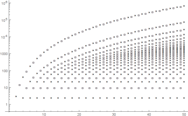
Figure 1. Distribution of the roots of $F_{n}(\lambda)$ for $2\leq n\leq 50$ on a logarithmic scale; for even $n$ the locations of the roots are marked by crosses, for odd $n$ with squares.

Proposition 5.1.

Let $F_{n}(\lambda)$ be defined as in (12) and let $\lambda^{(0)}_{n,1}<\dots<\lambda^{(0)}_{n,n}$ denote the roots of $F_{2n}(\lambda)$ in increasing order, and similarly $\lambda^{(1)}_{n,1}<\dots<\lambda^{(1)}_{n,n}$ denote the roots of $F_{2n+1}(\lambda)$. Then for fixed $k\in\mathbb{N}$ we have

$$\lim_{n\to\infty}\lambda^{(0)}_{n,k}=\bigl{(}k-\tfrac{1}{2}\bigr{)}^{2}\pi^{2}\qquad\text{and}\qquad\lim_{n\to\infty}\lambda^{(1)}_{n,k}=k^{2}\pi^{2}.$$

Proof.

The coefficient of $\lambda^{j}$ in $F_{2n}(\lambda)$ is, according to (12), given by

$$\frac{(-4)^{j-n}(2n-2j+1)_{2n}}{(2j)!}.$$

We normalize the monic polynomials $F_{2n}$ such that their constant coefficient is $1$, i.e., we divide $F_{2n}$ by $(-4)^{-n}(2n+1)_{2n}$, and obtain for the coefficient of $\lambda^{j}$ in these normalized polynomials:

$$\frac{(-4)^{j}(2n-2j+1)_{2n}}{(2j)!(2n+1)_{2n}}=\frac{(-1)^{j}}{(2j)!}\cdot\frac{4^{j}(2n-2j+1)_{2j}}{(4n-2j+1)_{2j}}.$$

Obviously the second factor is, for fixed $j$, a rational function in $n$ with numerator and denominator having the same degree $2j$ and the same leading coefficient $16^{j}$; hence it tends to $1$ as $n$ goes to infinity. This means that the power series obtained as the limit of the normalized polynomials is

$$\sum_{j=0}^{\infty}\frac{(-1)^{j}}{(2j)!}x^{j}=\cos(\sqrt{x})$$

whose roots are precisely the limiting values in the assertion. The limit of $F_{2n+1}(\lambda)$ can be computed analogously and yields the Taylor expansion of $\sin(\sqrt{x})/\sqrt{x}$. ∎

Recall that we are actually not interested in the smallest root of $F_{n}(\lambda)$ but in the largest one. Its asymptotic behaviour can be extracted in a similar fashion.

Proposition 5.2.

Let $F_{n}(\lambda)$ be defined as in (12) and let $\lambda_{n}$ denote the largest root of $F_{n}$, as before. Then

$$\lim_{n\to\infty}\frac{\lambda_{n}}{n^{4}}=\frac{1}{\pi^{2}}.$$

Proof.

Let $\hat{F}_{n}(\lambda)$ denote the reciprocal polynomial of $F_{n}(\lambda)$, which means that $\hat{F}_{n}(\lambda)=\lambda^{\nu(n)}F_{n}(1/\lambda)$ where $\nu(n)=\lfloor n/2\rfloor$ is the degree of $F_{n}$. Then the largest root of $F_{n}$ equals the reciprocal of the smallest root of $\hat{F}_{n}$. Now consider the family of polynomials

$$\hat{F}_{n}\left(\frac{\lambda}{n^{4}}\right)=\sum_{j=0}^{\nu(n)}\frac{(2j+1)_{n}}{(-4n^{4})^{j}\,(n-2j)!}\lambda^{j}.$$

The coefficient of $\lambda^{j}$ in these polynomials tends to $(-4)^{-j}/(2j)!$ as $n$ goes to infinity. Hence in the limit we obtain the power series

$$\sum_{j=0}^{\infty}\frac{x^{j}}{(-4)^{j}\,(2j)!}=\cos\left(\frac{\sqrt{x}}{2}\right),$$

whose smallest root is $\pi^{2}$. The claim follows. ∎

Note that this result is in accordance with the bounds derived in Section 4, in particular with the inequality stated at the end of that section: the numerical value of $8\pi^{-2}$ is approximately $0.810569$ which is very close to the previously derived upper bound. The reason why the upper bound is more accurate comes from the fact that a third-degree approximation of $F_{n}(\lambda)$ was taken (in Lemma 4.8), whereas the lower bound was obtained from a second-degree polynomial (see Lemma 4.5).

6. The Boundary Estimate

Finally we tackle the second kind of problem, corresponding to Equation (4). In this instance it is advantageous to formulate it using the Legendre basis. Thus we have to solve the eigenvalue problem

$$L_{n}\underline{x}_{n}=\mu_{n}M_{n}\underline{x}_{n}$$

with the following $n\times n$ matrices $L_{n}$ and $M_{n}$: the $(i,j)$ entry of $L_{n}$ is given by

$$P_{i}(1)P_{j}(1)+P_{i}(-1)P_{j}(-1)$$

whereas in $M_{n}$ one has

$$\int_{-1}^{1}P_{i}(x)P_{j}(x)\,\mathrm{d}x.$$

Here the basis functions are the venerable Legendre polynomials $P_{n}(x)$. Taking into account the well-known evaluations $P_{n}(1)=1$ and $P_{n}(-1)=(-1)^{n}$ this is equivalent to finding the roots of the determinant of $C_{n}=(c_{i,j})_{1\leq i,j\leq n}$ whose matrix entries are given by

$$c_{i,j}:=1+(-1)^{i+j}-\delta_{i,j}\frac{2\mu}{2i+1}.$$

Obviously the matrix $C_{n}$ has zeros at all positions $(i,j)$ for which $i+j$ is an odd integer. As in Section 3 we decompose it into block form and obtain

$$\det(C_{n})=\begin{vmatrix}C^{(0)}_{\lfloor n/2\rfloor}&0\\ 0&C^{(1)}_{\lceil n/2\rceil}\end{vmatrix}=\det\Bigl{(}C^{(0)}_{\lfloor n/2\rfloor}\Bigr{)}\cdot\det\Bigl{(}C^{(1)}_{\lceil n/2\rceil}\Bigr{)}$$

where the subscripts indicate the dimension of the square matrices $C^{(0)}$ and $C^{(1)}$, whose entries are independent of the dimension and given by

$$c^{(0)}_{i,j}:=2-\delta_{i,j}\frac{2\mu}{4i+1}\quad\text{and}\quad c^{(1)}_{i,j}:=2-\delta_{i,j}\frac{2\mu}{4i-1}.$$

Theorem 6.1.

For all nonnegative integers $n$ we have

$$\det\bigl{(}C^{(0)}_{n}\bigr{)} =\frac{(-1)^{n}}{2^{n}\left(\frac{5}{4}\right)_{n}}\mu^{n-1}\bigl{(}\mu-2n^{2}-3n\bigr{)},$$

$$\det\bigl{(}C^{(1)}_{n}\bigr{)} =\frac{(-1)^{n}}{2^{n}\left(\frac{3}{4}\right)_{n}}\mu^{n-1}\bigl{(}\mu-2n^{2}-n\bigr{)}.$$

Proof.

By some elementary row operations, the matrix $C^{(0)}_{n}$ is brought to triangular form. First we subtract the first row from rows $2$ through $n$, obtaining the following matrix: the $(1,1)$ entry is $2-\frac{2\mu}{5}$, the remaining entries in the first row are $2$, the remaining entries of the first column are $\frac{2\mu}{5}$, and the diagonal entries $(i,i)$ are $-\frac{2\mu}{4i+1}$ for $i>1$; the rest are zeros. So in order to transform the matrix to lower triangular form, we multiply row $i$, for $2\leq i\leq n$, by $\frac{4i+1}{\mu}$ and add it to the first row. Thus the $(1,1)$-entry becomes

$$2-\frac{2\mu}{5}+\sum_{i=2}^{n}\frac{2\mu}{5}\frac{4i+1}{\mu}=\frac{2}{5}\bigl{(}2n^{2}+3n-\mu\bigr{)}.$$

It follows that the determinant of $C^{(0)}_{n}$ is

$$\frac{2}{5}\bigl{(}2n^{2}+3n-\mu\bigr{)}\prod_{i=2}^{n}\frac{-2\mu}{4i+1}=\frac{(-1)^{n}}{2^{n}\left(\frac{5}{4}\right)_{n}}\mu^{n-1}\bigl{(}\mu-2n^{2}-3n\bigr{)},$$

as claimed. The evaluation of $\det\bigl{(}C^{(1)}_{n}\bigr{)}$ is obtained in a completely analogous way. ∎

Corollary 6.2.

For all nonnegative integers $n$ we have

$$\det(C_{n}) =\det_{1\leq i,j\leq n}\Bigl{(}1+(-1)^{i+j}-\delta_{i,j}\frac{2\mu}{2i+1}\Bigr{)}$$

$$=\frac{(-1)^{n}}{\left(\frac{3}{2}\right)_{n}}\mu^{n-2}\Bigl{(}\mu-2\left\lfloor\frac{n}{2}\right\rfloor^{2}-3\left\lfloor\frac{n}{2}\right\rfloor\Bigr{)}\Bigl{(}\mu-2\left\lceil\frac{n}{2}\right\rceil^{2}-\left\lceil\frac{n}{2}\right\rceil\Bigr{)}$$

$$=\frac{(-1)^{n}}{\left(\frac{3}{2}\right)_{n}}\mu^{n-2}\begin{cases}\bigl{(}\mu-\frac{n^{2}+3n}{2}\bigr{)}\bigl{(}\mu-\frac{n^{2}+n}{2}\bigr{)},&\text{if }n\text{ is even},\\ \bigl{(}\mu-\frac{n^{2}+3n+2}{2}\bigr{)}\bigl{(}\mu-\frac{n^{2}+n-2}{2}\bigr{)},&\text{if }n\text{ is odd}.\end{cases}$$

The previous corollary now gives an answer to the original eigenvalue problem, namely that the largest eigenvalue $\mu_{n}$ of $L_{n}\underline{x}_{n}=\mu_{n}M_{n}\underline{x}_{n}$ is

$$\mu_{n}=\begin{cases}\frac{1}{2}n(n+3)&\text{if }n\text{ is even},\\ \frac{1}{2}n(n+3)+1&\text{if }n\text{ is odd}.\end{cases}$$

7. Outlook and future work

In this work we have presented tools from symbolic computation to give precise estimates for two types of inverse inequalities. It would be interesting to apply these methods on other types of elements, like simplices for example. Moreover, in Isogeometric Analysis (IgA) the constants in the inverse inequalities depend on three parameters, i.e. the mesh size, the polynomial degree and the smoothness factor. For this case not so much is known and it would be attractive to apply tools from symbolic computation also in this case.

Acknowledgment

We are grateful to Ulrich Langer for initiating this collaboration between the Numerical Analysis Group and the Symbolic Computation Groups at JKU, RISC, and RICAM. We want to thank Peter Paule for insightful discussions on the properties of the polynomials $F_{n}(\lambda)$. We also thank both of them for constantly motivating us to put a serious effort into solving this important problem. Last but not least we appreciate the careful reading and the helpful comments of the anonymous referee.

References

- [1] A. Bećirović, P. Paule, V. Pillwein, A. Riese, C. Schneider, J. Schöberl, Hypergeometric summation algorithms for high order finite elements, Computing 78 (2006) 235–249.
- [2] S. C. Brenner, L.R. Scott, The mathematical theory of finite element methods, Texts in Applied Mathematics, vol. 15, Springer, New York, third edition, 2008.
- [3] A.-L. Cauchy, Mémoire sur les fonctions alternées et sur les sommes alternées, in: Exercices d’Analyse et de Physique Mathématique, vol. 2, Bachelier, 1841, pp. 151–159.
- [4] P. G. Ciarlet, The finite element method for elliptic problems, Studies in Mathematics and its Applications, vol. 4, North-Holland Publishing Co., Amsterdam-New York-Oxford, 1978.
- [5] G. E. Collins, Quantifier elimination for the elementary theory of real closed fields by cylindrical algebraic decomposition, Lecture Notes in Computer Science 33 (1975) 134–183.
- [6] D. A. Di Pietro, A. Ern, Mathematical aspects of discontinuous Galerkin methods, Mathématiques & Applications (Berlin) [Mathematics & Applications], vol. 69, Springer, Heidelberg, 2012.
- [7] E. H. Georgoulis, Inverse-type estimates on -finite element spaces and applications, Math. Comp. 77 (2008) 201–219.
- [8] S. Gerhold, M. Kauers, A procedure for proving special function inequalities involving a discrete parameter, in: Proceedings of the International Symposium on Symbolic and Algebraic Computation (ISSAC), ACM, New York, USA, 2005, pp. 156–162.
- [9] I. G. Graham, W. Hackbusch, S. A. Sauter, Finite elements on degenerate meshes: inverse-type inequalities and applications, IMA J. Numer. Anal. 25 (2005) 379–407.
- [10] W. Hackbusch, Multigrid methods and applications, Springer Series in Computational Mathematics, vol. 4, Springer-Verlag, Berlin, 1985.
- [11] C. Koutschan, Advanced applications of the holonomic systems approach, PhD thesis, Research Institute for Symbolic Computation (RISC), Johannes Kepler University, Linz, Austria, 2009.
- [12] C. Koutschan, HolonomicFunctions (user’s guide), Technical Report 10-01, RISC Report Series, Johannes Kepler University, Linz, Austria, 2010. http://www.risc.jku.at/research/combinat/software/HolonomicFunctions/.
- [13] C. Koutschan, Electronic supplementary material for the paper “Inverse inequality estimates with symbolic computation”, 2016. Available at http://www.koutschan.de/data/maxeig/.
- [14] C. Koutschan, M. Kauers, D. Zeilberger, Proof of George Andrews’s and David Robbins’s -TSPP conjecture, Proceedings of the National Academy of Sciences 108 (2011) 2196–2199.
- [15] C. Koutschan, C. Lehrenfeld, J. Schöberl, Computer algebra meets finite elements: an efficient implementation for Maxwell’s equations, in: U. Langer, P. Paule, (Eds.), Numerical and Symbolic Scientific Computing: Progress and Prospects, Texts & Monographs in Symbolic Computation, Springer, Wien, 2012, pp. 105–121.
- [16] C. Koutschan, T. Thanatipanonda, Advanced computer algebra for determinants, Annals of Combinatorics 17 (2013) 509–523.
- [17] C. Krattenthaler, Advanced determinant calculus: A complement, Linear Algebra and its Applications 411 (2005) 68–166.
- [18] G. Kuperberg, Symmetry classes of alternating-sign matrices under one roof, Annals of Mathematics 156 (2002) 835–866.
- [19] S. Özışık, B. Rivière, T. Warburton, On the constants in inverse inequalities in , Technical Report TR10-19, Computational and Applied Mathematics Department, Rice University, 2010.
- [20] V. Pillwein, Symbolic computation and finite element methods, in: V. P. Gerdt, W. Koepf, W. M. Seiler, E. V. Vorozhtsov, (Eds.), CASC 2015, Lecture Notes in Computer Science (LNCS), vol. 9301, Springer-Verlag Berlin Heidelberg, 2015, pp. 374–388.
- [21] V. Pillwein S. Takacs, A local Fourier convergence analysis of a multigrid method using symbolic computation, Journal of Symbolic Computation 63 (2014) 1–20.
- [22] C. Schwab, - and -finite element methods, theory and applications in solid and fluid mechanics, Numerical Mathematics and Scientific Computation, The Clarendon Press, Oxford University Press, New York, 1998.
- [23] U. Trottenberg, C. W. Oosterlee, A. Schüller, Multigrid, Academic Press, Inc., San Diego, CA, 2001.
- [24] R. Verfürth, On the constants in some inverse inequalities for finite element functions, Technical report, Fakultät für Mathematik, Ruhr-Universität Bochum, 2004.
- [25] T. Warburton, J. S. Hesthaven, On the constants in -finite element trace inverse inequalities, Comput. Methods Appl. Mech. Engrg. 192 (2003) 2765–2773.
- [26] D. Zeilberger, A holonomic systems approach to special functions identities, Journal of Computational and Applied Mathematics 32 (1990) 321–368.
- [27] D. Zeilberger, The holonomic ansatz II. Automatic discovery(!) and proof(!!) of holonomic determinant evaluations, Annals of Combinatorics 11 (2007) 241–247.