Charge dynamics of the antiferromagnetically ordered Mott insulator

Abstract

We introduce a slave-fermion formulation in which to study the charge dynamics of the half-filled Hubbard model on the square lattice. In this description, the charge degrees of freedom are represented by fermionic holons and doublons and the Mott-insulating characteristics of the ground state are the consequence of holon-doublon bound-state formation. The bosonic spin degrees of freedom are described by the antiferromagnetic Heisenberg model, yielding long-ranged (Néel) magnetic order at zero temperature. Within this framework and in the self-consistent Born approximation, we perform systematic calculations of the average double occupancy, the electronic density of states, the spectral function and the optical conductivity. Qualitatively, our method reproduces the lower and upper Hubbard bands, the spectral-weight transfer into a coherent quasiparticle band at their lower edges and the renormalisation of the Mott gap, which is associated with holon-doublon binding, due to the interactions of both quasiparticle species with the magnons. The zeros of the Green function at the chemical potential give the Luttinger volume, the poles of the self-energy reflect the underlying quasiparticle dispersion with a spin-renormalised hopping parameter and the optical gap is directly related to the Mott gap. Quantitatively, the square-lattice Hubbard model is one of the best-characterised problems in correlated condensed matter and many numerical calculations, all with different strengths and weaknesses, exist with which to benchmark our approach. From the semi-quantitative accuracy of our results for all but the weakest interaction strengths, we conclude that a self-consistent treatment of the spin fluctuation effects on the charge degrees of freedom captures all the essential physics of the antiferromagnetic Mott-Hubbard insulator. We remark in addition that an analytical approximation with these properties serves a vital function in developing a full understanding of the fundamental physics of the Mott state, both in the antiferromagnetic insulator and at finite temperatures and dopings.

Keywords: Hubbard model, Mott insulator, holon-doublon binding, spin fluctuations

1 Introduction

The mechanism underlying the Mott metal-insulator transition [1] stands as a fundamental theoretical challenge in condensed matter physics. In 1937, de Boer and Verwey [2] reported that a class of transition-metal oxides with partially filled bands, specifically NiO and MnO, are semiconductors or insulators in direct contradiction to predictions by conventional band theory. This motivated Mott and Peierls [3] to point out the importance of the electrostatic interaction between the electrons, and Mott later introduced the concept of the metal-insulator transition that bears his name [4, 5] to describe insulating behaviour arising as a result of strong electron-electron correlations. The discovery of high-$T_{c}$ superconductivity in a class of doped antiferromagnetic Mott insulators [6] revived an enormous and lasting interest in understanding the Mott phase and the associated metal-insulator transition.

The Hubbard model [7] is the minimal model describing the competition between the kinetic energy of the electrons and their on-site Coulomb interaction. It captures many characteristic features of strongly correlated systems and thus serves as a paradigm for numerous phenomena in condensed matter physics. It is believed that the Hubbard model contains all the basic physics of the Mott metal-insulator transition and, in some quarters, that it may reveal the mechanism of high-$T_{c}$ superconductivity. However, despite the simplicity of the Hubbard model, exact results can be obtained only from the Bethe Ansatz [8] in one dimension and from Dynamical Mean-Field Theory (DMFT) [9, 10] in infinite dimensions.

There exist many proposals for the primary mechanism driving the Mott transition. Hubbard’s equation-of-motion methods [7, 11, 12, 13, 14] attribute the charge gap to the formation of the incoherent lower and upper Hubbard bands. These provided the first example for a metal-insulator transition in which the insulating behaviour is not accompanied by the onset of magnetic order. Brinkman and Rice [15] applied the Gutzwiller variational method [16] to treat the metal-insulator transition out of the Fermi-liquid metallic phase, and ascribed the transition to the vanishing of the quasiparticle residue, $Z$, and the divergence of the quasiparticle effective mass, $m^{\ast}$. The Hubbard approximation captures the incoherent part of the physics while the Brinkman-Rice approximation captures the coherent part. However, neither approximation takes the effect of spin fluctuations into account.

For the half-filled single-band Hubbard model on the square lattice, quantum Monte Carlo simulations [17, 18] have shown that the ground state is an antiferromagnetic insulator, although by the Mermin-Wagner theorem its Néel temperature is zero. In the weak-coupling limit, Fermi-surface nesting and the proximity to a van Hove singularity in the density of states act to induce a spin-density-wave state and thus to produce a gap [17]. An asymptotically exact weak-coupling solution for the Hubbard model was given in reference [19]. In the strong-coupling regime, it is the large on-site Coulomb repulsion energy, $U$, for double site occupancy that suppresses electron mobility and determines the Mott gap.

For the intermediate-coupling regime, where no well-controlled theoretical solution exists, many numerical methods have been applied to the two-dimensional (2D) Hubbard model, including exact diagonalisation [20, 22, 21, 23, 24], quantum Monte Carlo [25, 26, 27, 28, 29, 30, 31, 32], cluster perturbation theory [33, 34, 35, 36, 37, 38], the variational cluster approximation [39, 40, 41, 42, 43] and cluster DMFT [44, 45, 46, 47, 48, 49]. A detailed review, including further results from density-matrix renormalisation-group (DMRG) calculations, may be found in reference [50]. However, all of these methods suffer from different intrinsic limitations. Cluster perturbation theory provides an approximate lattice Green function for a continuous wave-vector space but is not self-consistent and cannot describe broken-symmetry states, which are known to be present for the half-filled square lattice. The variational cluster approximation can be viewed as an extension of cluster perturbation theory, which allows for broken symmetries by introducing Weiss fields, but remains limited by the cluster size. In cluster DMFT, the quantum impurity model can be solved by quantum Monte Carlo or exact diagonalisation. The former operates at finite temperature and imaginary time, requiring extrapolation to recover zero-temperature information and analytic continuation methods to obtain real-frequency results, neither of which is well controlled; further, the ubiquitous fermion sign problem affecting quantum Monte Carlo methods becomes severe when the system is doped. The latter is implemented at zero temperature and gives direct real-frequency dynamical information, but can access only small cluster sizes. DMRG is inherently 1D in nature and can be applied only on a narrow cylinder; the ongoing development of higher-dimensional analogues based on tensor-network states has progressed to the point where an infinite projected entangled-pair state (iPEPS) method has been used very recently to obtain very competitive ground-state energies [51]. Anderson [52] has argued that the half-filled 2D Hubbard model is fundamentally nonperturbative in nature, in the same way as the 1D case, with a Mott gap present for all $U>0$ and robust against temperature. Thus despite all of the theoretical and numerical progress made to date, the nature of the Mott gap at half-filling and the properties of the 2D Hubbard model remain as challenging open questions.

In the strong-coupling limit, below half-filling the dominant on-site Coulomb repulsion implies the absolute exclusion of doubly occupied sites. In this case, the Hubbard model can be mapped to the $t$–$J$ model at the level of second-order perturbation theory [53]. At half-filling, no empty sites remain and this model reduces to the antiferromagnetic Heisenberg model with only spin-fluctuation degrees of freedom. As $U$ decreases, charge fluctuations play an increasingly important role in the Hubbard model [54, 55], and in the half-filled case the elementary charge excitations are holons (empty sites) and doublons (doubly occupied sites), in equal numbers. However, even at weak coupling, insulating behavior remains guaranteed if the holons and doublons have a tendency to form bound states, which results in the presence of a charge gap. Variational Monte Carlo results [56, 57, 58, 59, 60] have shown that a variational wave function including holon-doublon binding effects can lower the ground-state energy and that the Mott transition can be characterised as an unbinding transition of holons and doublons. Several theoretical proposals for the mechanism of Mott physics contain holon-doublon binding as an important element, including the “hidden charge-2e boson” mechanism [61, 62, 63], the reconstruction of poles and zeros of the Green function [64, 65, 66], composite fermion theory [67] and the Kotliar-Ruckenstein slave-boson theory [68]. The zeros of the Green function at the chemical potential in momentum space can be taken to define the “Luttinger surface,” which is closely connected to the non-interacting Fermi surface [69].

The motion of a single hole in an antiferromagnetic background has been studied extensively within the self-consistent Born approximation (SCBA) [70, 71, 72, 73, 74, 75], where the neglect of Feynman diagrams with crossing propagators is equivalent to neglecting the distortion of the spin background caused by the presence of the hole. This formulation is similar to the retraceable path (Brinkman-Rice) approximation [76] and the resulting single-hole spectral function is composed of two components, a sharp peak corresponding to coherent quasiparticle motion and an incoherent background. The coherent peak arises from the coupling between the hole and the spin excitations. Recent experiments have shown that the SCBA yields excellent agreement with resonant inelastic X-ray scattering measurements performed on the quasi-2D spin-$1/2$ antiferromagnet Sr₂IrO₄ [77].

To make a meaningful contribution to such a complex and deeply studied problem, here we aim to provide an analytical framework which captures the essential features of the charge dynamics of the single-band Hubbard model. To introduce this framework, we restrict our considerations to the square-lattice model with only nearest-neighbour coupling, to half-filling, and to zero temperature. While it is unrealistic to expect to find much new physics in this most generic situation, our goals are to demonstrate the qualitative power of a suitably chosen mean-field description, to establish the semi-quantitative accuracy of our results by benchmarking against the plethora of available numerical studies, and to lay a foundation for development in the more experimentally relevant directions of finite temperatures, extended bandstructures and finite dopings.

An accurate description of the Mott insulator is based on the strong-coupling limit, where its properties are robust. As we discuss in more detail below, this leads to a formalism where the charge degrees of freedom are represented by fermionic holons and doublons and the Mott-insulating state involves the formation of holon-doublon bound states. The spin degrees of freedom, represented by bosonic magnons, order magnetically at zero temperature for any finite interaction strength, but their quantum fluctuations act to renormalise the charge sector. Thus the task at hand is to consider the antiferromagnetically ordered Mott insulator and to describe accurately both the holon-doublon binding process and the spin renormalisation of the charge dynamics.

For specificity, we declare here that we take the on-site interaction to be the origin of Mott physics for all dimensionalities, temperatures or dopings, and antiferromagnetic fluctuations to be one consequence. It is true that this assumption remains unproven for the square lattice (2D) with nearest-neighbour hopping at half-filling: in this somewhat pathological case, the perfect Fermi-surface nesting means that a gap is opened in the charge sector at any finite interaction strength, and in a weak-coupling picture this can be interpreted as a process driven by the onset of antiferromagnetic order, i.e. not by the charge sector but by the spin sector. This result has led to significant confusion over whether an antiferromagnetic insulator can exist independently of a Mott insulator. We use the fact that there is no transition at any finite interaction strength in the model at hand to deduce that the two possible states are different manifestations of the same physics and are connected by a crossover. For practical purposes, here we take the extensive numerical calculations on the half-filled Hubbard model to indicate that the ground state is a magnetically ordered Mott insulator for all intermediate (and experimentally relevant) interaction strengths. The Mott (charge excitation) gap in our framework is a consequence of holon-doublon binding and its presence ensures a finite spectral (single-particle excitation) gap, while the spin excitations are gapless. The same holon-doublon binding mechanism is equally applicable to the Hubbard model at finite temperature or doping, where the spin sector is present only as short-range fluctuations.

Our approach is based on a slave-particle formalism [78, 79, 80, 81, 82] in which electron operators are expressed as a combination of “slave” fermionic and bosonic operators preserving the net fermionic statistics, and spin-charge separation is assumed. A degree of arbitrariness exists in ascribing the fermionic statistics to the spin (known as the slave-boson approach) or to the charge degrees of freedom (slave-fermion decomposition). Keeping the importance of spin fluctuations at the forefront of our considerations, we assume that the ground state has Néel order, which is known in the large-$U$ limit, and that the spin degrees of freedom are described by the antiferromagnetic Heisenberg model. The ground state of this model on the square lattice for $S=1/2$ is better described by the Schwinger boson (slave-fermion) formulation [81, 84]. Of equal importance, for an investigation of the holon-doublon binding mechanism it is physically much more intuitive to ascribe the fermionic statistics to the charge degrees of freedom, in analogy with the electron binding mechanism of Bardeen-Cooper-Schrieffer (BCS) superconductivity.

In this slave-fermion framework, antiferromagnetic long-range order corresponds to the condensation of one of the slave bosons on each sublattice in the ground state. On this basis, we treat the spin dynamics within the linear spin-wave approximation [53], where the elementary excitations are magnons. Because the motion of holons and doublons distorts the antiferromagnetic background even at half-filling, a consistent account of spin-fluctuation effects is of key importance in describing the charge dynamics. We treat the interactions among holons, doublons and magnons within the SCBA to calculate important physical quantities including the double occupancy, the spectral function, the electronic density of states, the quasiparticle Green function and the optical conductivity. Our results show a non-zero double occupancy for any finite $U$, that the Mott-insulating state results from holon-doublon binding, that spin fluctuations modify the size of the Mott gap and that this gap can be probed accurately by measurements of the optical conductivity.

This paper is organised as follows. In section 2 we introduce formally the model and the methods we use to perform our calculations. In section 3 we compute the doublon density for all intermediate values of $U$ and in section 4 we present the spectral function to discuss the coherent and incoherent components of the charge response, the density of states and the Mott gap. In section 5 we calculate the electron Green function and associated Luttinger surface, and deduce the effective quasiparticle bandstructure. Section 6 contains our results for and conclusions from the optical conductivity and a summary is provided in section 7.

2 Model and Method

The single-band Hubbard model is defined by the Hamiltonian

$$H=-t\sum_{\langle i,j\rangle\sigma}c_{i\sigma}^{\dagger}c_{j\sigma}+U\sum_{i}(n_{i\uparrow}-1/2)(n_{i\downarrow}-1/2),$$ (1)

where $c_{i\sigma}$ ($c_{i\sigma}^{\dagger}$) denotes the annihilation (creation) operator of an electron with spin $\sigma$ on site $i$ of the square lattice and $\langle i,j\rangle$ indicates that we restrict the hopping terms to nearest-neighbour sites $i$ and $j$ only. We set the hopping parameter as $t=1$ to establish the energy units of our calculations and $U$ represents the on-site Coulomb repulsion.

In the slave-fermion formalism, the electron operator is written as

$$c_{i\sigma}=s_{i\overline{\sigma}}^{\dagger}d_{i}+\sigma e_{i}^{\dagger}s_{i\sigma},$$ (2)

where $d_{i}$ and $e_{i}$ are fermionic operators denoting the charge degrees of freedom and $s_{i\sigma}$ are bosonic operators describing the spin degrees of freedom, with $\sigma=1$ for spin $\uparrow$ and $-1$ for spin $\downarrow$. The operator $e_{i}^{\dagger}$ creates an empty (unoccupied) site, a holon, at lattice point $i$, $d_{i}^{{\dagger}}$ creates a doubly occupied site, a doublon, and $s_{i\sigma}^{\dagger}$ ($s_{i\bar{\sigma}}^{\dagger}$) is the creation operator for a singly occupied site $i$ with spin $\sigma$ ($\bar{\sigma}$). In this formulation, the local Hilbert space is enlarged and the constraint

$$d_{i}^{\dagger}d_{i}+e_{i}^{\dagger}e_{i}+\sum_{\sigma}s_{i\sigma}^{\dagger}s_{i\sigma}=1$$ (3)

should be satisfied to eliminate unphysical states.

Substituting equation (2) into equation (1) gives the form

$$H =-t\sum_{i,\delta,\sigma}[(d_{i+\delta}^{\dagger}d_{i}-e_{i+\delta}^{\dagger}e_{i})s_{i,\sigma}^{\dagger}s_{i+\delta,\sigma}+\rm{H}.\rm{c}.]$$ (4)

$$\quad-t\sum_{i,\delta,\sigma}[(d_{i}^{\dagger}e_{i+\delta}^{\dagger}+e_{i}^{\dagger}d_{i+\delta}^{\dagger})\sigma s_{i,\bar{\sigma}}s_{i+\delta,\sigma}+\rm{H}.\rm{c}.]$$

$$\quad+{\textstyle\frac{1}{2}}U\sum_{i}(d_{i}^{\dagger}d_{i}+e_{i}^{\dagger}e_{i}-{\textstyle\frac{1}{2}}),$$

where $\delta$ denotes the lattice vectors $(a,0)$ and $(0,a)$. Here we do not include a Lagrange-multiplier term to enforce the local constraint at a global level (introducing a chemical potential), but instead implement equation (3) as a self-consistent condition in our treatment. This procedure has the same effect, in that the constraint is satisfied only on average, which is a primary shortcoming of all analytical approaches to locally constrained problems unless gauge fluctuations can be included. Otherwise, the efficacy of this type of approximation is difficult to assess by any means other than comparing the results it yields with numerical calculations where the constraint can be enforced exactly.

From the first line of equation (4), holons and doublons can hop between nearest-neighbour sites with accompanying creation and annihilation of singly-occupied states. This term serves as the starting point for applying the SCBA, which provides a proper treatment of the coupling between the charge degrees of freedom and the spin fluctuations [70, 71, 72, 73, 74, 75]. This procedure requires the assumption of a Néel-ordered ground state, which is equivalent to a Bose condensation of the $s_{i\sigma}^{\dagger}$ operators and is discussed in detail below. The second line of equation (4) shows that the kinetic term of the Hubbard model contains a pairing interaction between holons and doublons in the slave-fermion representation. As noted in section 1, the analogy with BCS theory motivates both the attribution of fermionic statistics to the charge degrees of freedom and the formation of bosonic bound pairs of fermionic holons and doublons as the process underlying the opening of a charge gap and contributing to the charge dynamics of the Mott insulator. In the last line of equation (4), the Coulomb repulsion, $U$, appears as a mass term for holons and doublons, which gain a dispersive nature both through their pairing and through their interactions with the magnetic background, as described by the SCBA.

As appropriate for a method based on the large-$U$ limit, we assume that the ground state for the spin degrees of freedom is the Néel antiferromagnet, also for finite $U$, and that their fluctuations are described by the antiferromagnetic Heisenberg Hamiltonian,

$$H_{S}=J\sum_{\langle i,j\rangle}\mathbf{S}_{i}\cdot\mathbf{S}_{j},$$ (5)

with the coupling constant taken for simplicity as $J=4t^{2}/U$. In the Schwinger boson representation, the spin operators are given by

$$\mathbf{S}_{i}=\frac{1}{2}\sum_{\alpha\beta}s_{i\alpha}^{\dagger}\boldsymbol{\sigma}_{\alpha\beta}s_{i\beta},$$ (6)

where $\boldsymbol{\sigma}=(\sigma^{x},\sigma^{y},\sigma^{z})$ denotes the Pauli matrices. The Néel antiferromagnetic state corresponds to a Bose-Einstein condensation of one of the two types of bosonic operator on each sublattice [83], which we describe by the uniform mean-field assumption

$$s_{i\uparrow}^{\dagger},s_{i\uparrow} \longrightarrow\langle s_{i\uparrow}\rangle=\langle s_{i\uparrow}^{\dagger}\rangle=b_{0},\qquad i\in A,$$

$$s_{j\downarrow}^{\dagger},s_{j\downarrow} \longrightarrow\langle s_{j\downarrow}\rangle=\langle s_{j\downarrow}^{\dagger}\rangle=b_{0},\qquad j\in B,$$ (7)

for the two sublattices $A$ and $B$. The constraint (3) is then recast as

$$b_{0}^{2}=\left\{\begin{array}[c]{c}1-\langle d_{i}^{\dagger}d_{i}\rangle-\langle e_{i}^{\dagger}e_{i}\rangle-\langle s_{i\downarrow}^{\dagger}s_{i\downarrow}\rangle,\\ 1-\langle d_{i}^{\dagger}d_{i}\rangle-\langle e_{i}^{\dagger}e_{i}\rangle-\langle s_{j\uparrow}^{\dagger}s_{j\uparrow}\rangle,\end{array}\right.\begin{array}[c]{c}i\in A,\\ j\in B.\end{array}$$ (8)

Because there is only one Schwinger boson on each sublattice, henceforth we simplify the notation $s_{i\sigma}$ to $s_{i}$. The revised form (8) of the constraint is the self-consistency condition in our calculation. We include the spin excitations of the antiferromagnetic Heisenberg model using the straightforward linear spin-wave approximation; although this method is only valid strictly for large spin and high-dimensional lattice geometries, it has been shown [84] that physical quantities, including the ground-state energy and sublattice magnetisation, obtained for the $S=1/2$ square-lattice model within this approximation are qualitatively correct and readily renormalised to the values given by numerical calculations. A more detailed treatment of the Heisenberg model is provided in A.1.

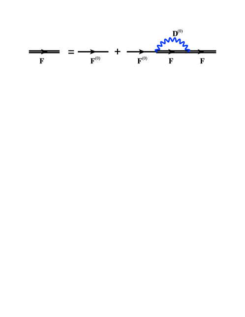
Figure 1: Feynman diagrams for the SCBA; fermion and magnon propagators are represented respectively by straight and wavy lines.

Within this approximation, equation (4) can be expressed as

$$H=\sum_{\mathbf{k}}\psi_{\mathbf{k}}^{\dagger}\tilde{\varepsilon}_{\mathbf{k}}\psi_{\mathbf{k}}+\sum_{\mathbf{k},\mathbf{q}}\psi_{\mathbf{k}}^{\dagger}M(\mathbf{k},\mathbf{q})\psi_{\mathbf{k}-\mathbf{q}},$$ (9)

where $\psi_{\mathbf{k}}^{\dagger}=(\!\!\begin{array}[c]{cc}d_{-\mathbf{k}+\mathbf{Q}}^{\dagger}&e_{\mathbf{k}}\end{array}\!)$ is the Nambu spinor, which contains the charge degrees of freedom. The explicit forms of $\tilde{\varepsilon}_{\mathbf{k}}$ and $M(\mathbf{k},\mathbf{q})$ may be found in A.2 along with full details of the SCBA for the Hubbard model in this form. The first term of equation (9) describes the unperturbed charge dynamics, with holon-doublon binding appearing in the off-diagonal part of the matrix. The second term describes the interaction between the charge and spin degrees of freedom. We define the full charge Matsubara Green function as

$$\mathbf{F}(\mathbf{k},\tau)=-\langle T_{\tau}\psi_{\mathbf{k}}(\tau)\psi_{\mathbf{k}}^{\dagger}(0)\rangle$$ (10)

and calculate this at the level of the SCBA. This process includes the coupling between the charge and spin dynamics and is equivalent to the series of Feynman diagrams shown in figure 1, where $\mathbf{F}^{(0)}$ and $\mathbf{F}$ are respectively the bare and interacting charge Green functions and $\mathbf{D}$ is the magnon Green function, whose explicit form is given in A.1. The SCBA has been used to calculate the motion of a single hole in an antiferromagnetic background in the $t$–$J$ model, where a consistent account of the mutual effects of charge motion and spin fluctuations is similarly essential. The results of these studies show that the coupling between the holon and the spin waves induces a quasiparticle-type response often labelled a spin polaron [70, 71, 72, 73, 74, 75]. Although a proper treatment of charge and spin fluctuations can be obtained in this way, we comment that the approximation does not include vertex corrections.

The self-consistent Dyson equation for the charge Green function is calculated by standard techniques, which yield

$$\mathbf{F}(\mathbf{k},i\omega_{n})=\frac{1}{i\omega_{n}-\tilde{\varepsilon}_{\mathbf{k}}-\mathbf{\Sigma}(\mathbf{k},i\omega_{n})},$$ (11)

where the self-energy $\mathbf{\Sigma}(\mathbf{k},i\omega_{n})$ is given in A.2. The retarded charge Green function can be obtained from the Matsubara Green function (10) by analytic continuation through $i\omega_{n}\rightarrow\omega+i\eta$. The effect of the parameter $\eta$ is to provide a finite width to peaks in the density of states.

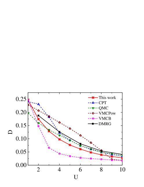
Figure 2: Double-occupancy parameter, $D$, shown as a function of on-site Coulomb repulsion, $U$. The solid, red line is our result, calculated for a system size of $48\times 48$ and with broadening parameter $\eta=0.08$. For comparison, the dashed lines show analogous results obtained from cluster perturbation theory (CPT, blue, up-pointing triangles) [86], quantum Monte Carlo (QMC) for a $4\times 4$ lattice at inverse temperature $\beta=16$ (green, down-pointing triangles) [18], variational Monte Carlo with different trial wave functions [$|\psi_{pow}\rangle$ (VMCPow, maroon diamonds) and $|\psi_{B}\rangle$ (VMCB, magenta squares) in the notation of reference [60]] and DMRG (solid, black line) with extrapolation to the thermodynamic limit [50].

3 Double occupancy

We begin the discussion of our results for the Mott-insulating state of the square-lattice Hubbard model by considering the averaged double-occupancy parameter, $D$. For the half-filled system, the average number of doubly occupied sites is equal to the number of empty ones, and is given by

$$D=\langle n_{d}\rangle=\frac{1}{N}\sum_{i}\langle d_{i}^{\dagger}d_{i}\rangle=\frac{1}{N}\sum_{i}\langle n_{i\uparrow}n_{i\downarrow}\rangle.$$ (12)

$D$ is exactly zero only when the on-site Coulomb repulsion, $U$ (1), is infinite, but charge fluctuations are intrinsic to the Hubbard model for all finite $U$ values, making $D$ finite. It therefore reflects average information about the effects of charge fluctuations and as such can be used to characterise the Mott transition [54, 58, 15, 85, 55, 59, 60].

The dependence of $D$ on $U$ at zero temperature is shown in figure 2, where our results are compared with calculations by quantum Monte Carlo [18], variational Monte Carlo [60], cluster perturbation theory [86] and DMRG [50]. At the qualitative level, all results lie in the same general range of values and, with the exception of one VMC approach, show a broadly similar functional form. Quantitatively, it is immediately clear that the different numerical results differ from each other quite significantly throughout the regions of weak and intermediate coupling, which may be taken as a signal of how difficult the Hubbard problem is in this regime. We stress that finite-size extrapolation of our results (not shown) confirms that our $48\times 48$ calculations are fully representative of the infinite system, whereas none of the numerical data shown in figure 2 have been extrapolated to the thermodynamic limit other than the DMRG results. However, extrapolated results obtained by a range of methods may be found in a very recent review [50].

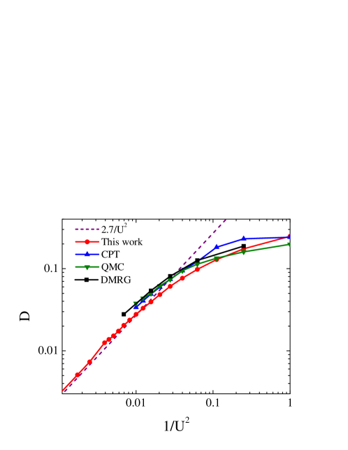
Figure 3: Double occupancy parameter, $D$, shown as a function of $1/U^{2}$ on logarithmic axes. Red points show our large-$U$ results, calculated for a system size of $48\times 48$ and with broadening parameter $\eta=0.08$. Results from CPT, QMC and DMRG, shown in the same colour and symbol scheme as in figure 2, confirm the trend towards the limiting large-$U$ functional form, $D=2.70/U^{2}$ (dashed purple line).

Only in the strong-coupling regime do the differences in $D$ values obtained from all of these methods become small. Not only is our result in full agreement here, but because it is constructed in the strong-coupling limit, it can be expected to give the correct asymptotic form of $D$ as $U$ becomes large. We have calculated $D$ in the SCBA for a number of large $U$ values up to $U=64$, which we show in figure 3. By considering the doublon Green function, $\mathbf{F}^{(0)}_{11}(k,\tau)=\langle d_{-k+Q}(\tau)\,d_{-k+Q}^{\dagger}(0)\rangle$, in the limit of large $U$ and extracting the zero-temperature doublon occupation from the spectral function according to $\langle d_{-k+Q}^{\dagger}d_{-k+Q}\rangle=\int_{-\infty}^{0}d\omega A^{(0)}(k,\omega)$, one obtains

$$D=\frac{4t^{2}b_{0}^{4}}{U^{2}}\frac{1}{N}\sum_{k}(\cos k_{x}+\cos k_{y})^{2}\simeq\frac{2.70}{U^{2}}.$$ (13)

Further details may be found in B.2. This asymptotic form is shown in figure 3, allowing us to conclude that the double occupation function is suppressed at large $U$ according to $D\propto 1/U^{2}$. The results from a number of independent numerical studies, also shown in figure 3 are fully consistent with $1/U^{2}$ scaling at large $U$.

At half-filling, the value of $D$ should change monotonically from 0 to $1/4$, which correspond respectively to the fully localised ($U=\infty$) and the completely delocalised cases ($U=0$). As $U$ decreases, charge fluctuations are enhanced and the on-site Coulomb interaction is screened, making localisation effects smaller and reducing the Mott gap. The result is larger $D$ values for smaller $U$, indicating an increasing mixing of the lower and upper Hubbard bands. Still, it is only at very small values, $U<2$, of the on-site repulsion that our results begin to indicate the breakdown of the approximation, which benchmarks the limits of its applicability. They do not approach $D=1/4$ at $U=0$, which is no surprise because neither the strong-coupling slave-fermion formalism nor the single-mode spin-wave approximation to a Néel antiferromagnetic ground state as a description of the spin dynamics is appropriate in this limit.

In general, it is not true that $D$ should increase continuously with decreasing $U$. In some variational Monte Carlo calculations [58, 60], the behaviour of $D$ appears to show an abrupt change at a critical interaction strength, $U_{c}$, which has been interpreted as a first-order Mott transition. However, neither our result nor those obtained from cluster perturbation theory [86], quantum Monte Carlo simulations [18], or DMRG [50] contain any evidence for a Mott transition at finite $U$. As a consequence of the perfect nesting, the nearest-neighbour square-lattice Hubbard model is a special case where even a weak-coupling treatment gives an insulating state for all $U$, i.e. $U_{c}=0$. As noted in section 1, this small-$U$ result has led to intense debate over the question of whether insulating behaviour could be driven by antiferromagnetism rather than by the Coulomb interaction, and whether there could be a transition between the two regimes at finite $U$. However, the result that $U_{c}=0$ in this model means that all values of $U$ are continuously connected to the strong-coupling limit, where the answers are clear. Indeed, detailed numerical calculations have recently been used to argue [43] that the model also has no Mott-Hubbard transition at any finite $U$ in the paramagnetic phase at low but finite temperatures, meaning that no other effective terms are generated. We conclude from our calculations of $D$ that the holon-doublon description yields the correct functional form and semi-quantitative accuracy throughout the regime of intermediate and strong coupling (specifically, $U>2$).

4 Spectral Function

4.1 Derivation and Calculation

We calculate the spectral function of the original electron operators, $c_{\mathbf{k}\sigma}$, which in the slave-fermion framework are decomposed into convolutions of the holon operator, $e$, the doublon operator, $d$, and the Schwinger boson operator, $s$. The electron Green function is defined by

$$G(\mathbf{k},\tau)=-\sum_{\sigma}\langle T_{\tau}c_{\mathbf{k}\sigma}(\tau)c_{\mathbf{k}\sigma}^{\dagger}(0)\rangle$$ (14)

and the spectral function

$$A(\mathbf{k},\omega)=-\frac{1}{\pi}\rm{I}\rm{m}G^{R}(\mathbf{k},\omega+i\eta),$$ (15)

the imaginary part of the retarded Green function, contains implicitly all information necessary to describe single-particle excitations. The electron density of states is obtained from the sum over all wavevectors,

$$\rho(\omega)=\frac{1}{N}\sum_{\mathbf{k}}A(\mathbf{k},\omega).$$ (16)

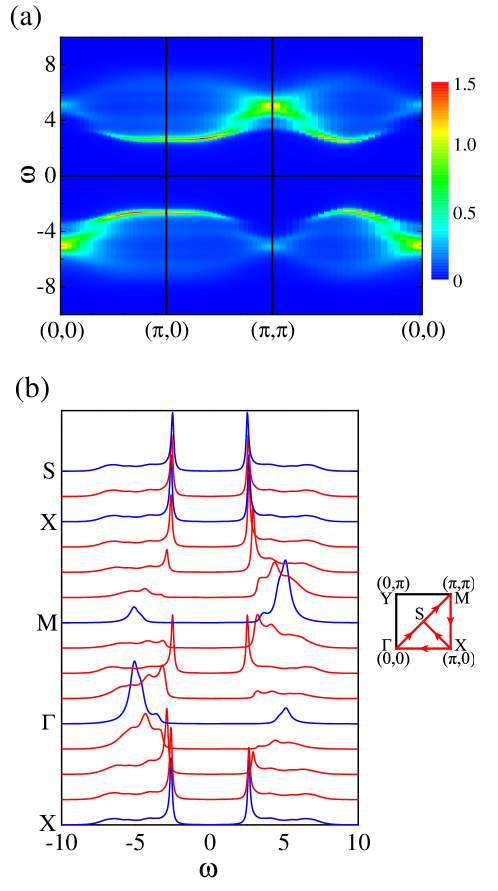
Figure 4: Electron spectral function, $A(\mathbf{k},\omega)$, of the Hubbard model with $U=8$, obtained for lattice dimensions $48\times 48$ and with broadening parameter $\eta=0.08$. (a) Spectral intensity along the symmetry directions $\Gamma\rightarrow$ M $\rightarrow$ X $\rightarrow\Gamma$ in the first quadrant of the first Brillouin zone. (b) Spectral function $A(\omega)$ for wavevectors $\mathbf{k}$ along the high-symmetry directions X $\rightarrow\Gamma\rightarrow$ M $\rightarrow$ X $\rightarrow$ S.

Figure 4 shows the single-particle spectral function, $A(\mathbf{k},\omega)$, for some specific high-symmetry directions in the Brillouin zone of the square lattice. These calculations were performed with $U=8$ on a $48\times 48$ lattice and we used a broadening parameter $\eta=0.08$; we stress again that this system size is effectively in the thermodynamic limit. The particle-hole symmetry of the spectral function, $A(\mathbf{k},\omega)=A(-\mathbf{k+Q},-\omega)$, with $\mathbf{Q}=(\pi,\pi)$, is preserved. It is clear from the spectral-intensity contour map of figure 4(a) that the spectral weight lies in two separate bands, the lower and upper Hubbard bands, which are separated by the Mott gap; this weight appears predominantly in the lower Hubbard band in regions of the Brillouin zone around $(0,0)$, and is transferred to the upper Hubbard band as $\mathbf{k}$ moves towards $(\pi,\pi)$.

We begin our comments on the nature of these results by noting that they are in quantitative agreement with calculations performed by the variational cluster approximation [40], in which the authors included long-range antiferromagnetic correlations by adding some Weiss fields. That we obtain the self-consistent interaction effects of the spin fluctuations on the charge degrees of freedom is one of the key qualitative features of our approach and will be discussed further below. The shifting of spectral weight between Hubbard bands signals that the real part of the electron Green function changes sign between $(0,0)$ and $(\pi,\pi)$, which implies that the self-energy diverges and the Green function has a zero surface falling within this region [64]. The importance of zeros and poles of the Green function has been stressed by many authors [24, 65, 66, 67, 87, 64] in the discussion of Mott physics, particularly in the context of pseudogap phenomena in the doped system. We defer a discussion of the zero surface of the electron Green function to section 5.

Results for the spectral function, $A(\omega)$, are shown in figure 4(b) for a sequence of wavevectors $\mathbf{k}$ along the high-symmetry directions of the Brillouin zone. The spectral function is always a multi-peak structure, and the four-peak form reported by references [28] and [40] is not very distinctive in our results. Most of the spectra consist of a peak at low energies, meaning closer to the chemical potential, accompanied by a broad, weak high-energy part. The low-energy peak can be interpreted as the coherent motion of the quasiparticles, which are formed from both holons and doublons and are renormalise by spin fluctuations. The high-energy part originates in incoherent charge excitations and forms the remainder of the Hubbard bands.

Returning to the details of figure 4(b), we observe that for $\mathbf{k}=(\pi,0)$ (the X point), the spectral weight is symmetrical about $\omega=0$. As $\mathbf{k}$ is moved along X $\rightarrow\Gamma$, weight is transferred from the positive- to the negative-$\omega$ regime, i.e. to lower energies, while along X $\rightarrow$ M the opposite happens; this behavior is a reflection of particle-hole symmetry. Because ($\pi,0$) lies on the noninteracting Fermi surface, when $\mathbf{k}$ lies inside this surface, most of the spectral weight has the properties of a particle, while outside it has the properties of a hole. An analogous spectral-weight redistribution is evident as $\mathbf{k}$ is moved from M to $\Gamma$, where the transfer is from positive to negative $\omega$. At $\mathbf{k}=(\pi/2,\pi/2)\equiv$ S, the distribution is again symmetrical in $\omega$ and the gap takes the minimum value obtained in our approximation. We note that all of these features are very similar to the results of exact diagonalisation [20, 22, 21, 23] and quantum Monte Carlo calculations [25, 26, 27, 28] of the Hubbard model at half-filling on the square lattice.

Clearly the leading momentum-dependence of the spectral function is the consequence of the underlying non-interacting electronic bands. Around X $\equiv(\pi,0)$, where this dispersion is rather flat [figure 4(a)], the high density of states and strong interactions are believed to be the origin of the pseudogap and Fermi-arc phenomena found in doped Hubbard models [36, 37]. To gauge how much of the momentum-dependence may be caused by the coupling between spin and charge degrees of freedom, we return to the question of the coherent and incoherent response. For the lower Hubbard band, there is an apparent suppression of spectral weight around $\omega\approx-3.5t$, visible near $\Gamma$, which separates the band into two parts. The “low-energy” part (meaning closer to $\omega=0$) is a quasiparticle-type band, which disperses from $\Gamma$ to S.

The emergence of a coherent quasiparticle band in the dynamical response is a highly nontrivial consequence of the interactions between the charge and spin sectors in the Hubbard model. In general, hole motion in a Néel ordered state is energetically unfavourable because the movement distorts the antiferromagnetic background. However, many calculations within the SCBA [70, 71, 72, 73, 74, 75] have shown that a quasiparticle, named the “spin polaron” [73, 74], forms as a result of holon-magnon coupling. The bandwidth of the spin polaron is governed by the spin exchange, $J$, and this feature forms the low-energy part of the lower Hubbard band. For the high-energy part, hole motion is thought to originate from effective three-site hopping processes [38], which allow hole propagation on the same sublattice that does not distort the antiferromagnetic background and therefore is less affected by spin fluctuations. We postpone a more detailed discussion of the Hubbard bands to the next section.

4.2 Density of States

The density of states, $\rho(\omega)$, obtained by integrating the spectral function is shown in figure 5, where we compare the results calculated in the SCBA with those of a simple holon-doublon mean-field approximation. The dominant feature in $\rho(\omega)$ is the strong Mott gap for the values of $U$ illustrated. In the mean-field results, shown in figure 5(a), the effects of spin fluctuations are neglected and the Mott gap is $U$. However, in our calculations [figure 5(b)] this gap is renormalised downwards, quite significantly at intermediate values of $U$. This renormalisation is related directly to the other significant feature of $\rho(\omega)$, the width of the lower and upper Hubbard bands, which clearly broadens (relative to $U$) as the on-site interaction decreases and spin fluctuations strengthen. As we will discuss in section 5, the bandwidth reflects the spin-related renormalisation of the underlying quasiparticle bands and may be treated as an effective hopping parameter, $t_{\rm eff}$, which is a fraction of the electron hopping parameter, $t$; by contrast, the Hubbard bands given by the mean-field approximation have a width given only by the spin interaction, $J=4t^{2}/U$, and therefore appear much narrower in figure 5(a).

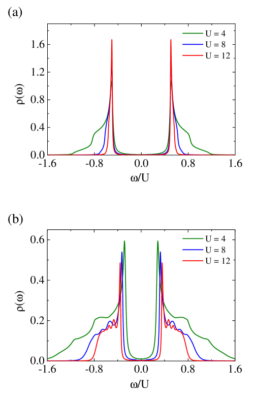
Figure 5: Electronic density of states, $\rho(\omega)$, shown for different values of $U$; data are normalised to $U$ on the frequency axis. A holon-doublon mean-field approximation (a) is compared with the results of the SCBA (b).

In the SCBA, only the quasiparticle band remains of width $J$. In general, the spin polaron is a feature of the retraceable path approximation [76] and is well-defined in a mean-field treatment with high lattice coordination. The energetics of the Mott gap and the Hubbard bands have been discussed in the DMFT, which is infinite-dimensional, and the same physics of a narrow quasiparticle band, a renormalised Mott gap and broader Hubbard bands is found [88]. That our 2D holon-doublon description reproduces these features with high accuracy serves both as an indication of the degree to which it captures the key ingredients of Mott physics and as a means to verify the relevance of features observed in numerical calculations with different limitations. In the context of DMFT comparisons, we caution that the small peaks visible around $\omega/U\approx 0.5$ in figure 5(b) are size effects, which we can demonstrate by smoothing them away if the broadening factor $\eta$ is set to a larger value.

Although a number of experiments have demonstrated the insulating behaviour of the parent compounds of the high-$T_{c}$ superconductors, it has proven to be very difficult to observe both the lower and upper Hubbard bands. Angle-resolved photoemission spectroscopy [89] probes the occupied states while optical spectroscopy [90, 91] gives information concerning two-particle correlations. Measurements by scanning tunnelling spectroscopy (STS) probe the local single-particle density of states for both occupied and unoccupied bands. Only recently was the full electronic spectrum for the undoped Mott insulator Ca₂CuO₂Cl₂ measured by STS [92], showing the Mott-Hubbard gap, and in particular the upper Hubbard band, for the first time. A comparison with the robust features of our results, namely the spin polaron, the renormalised Mott gap (section 4.3), and the width of the Hubbard bands scaling with $t$, implies that the Hubbard model does in fact capture the essential properties of the undoped Mott insulator measured by STS.

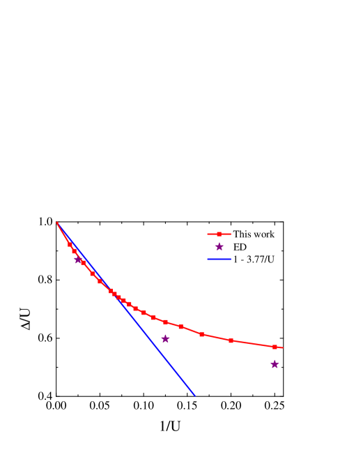
Figure 6: Mott gap, $\Delta$, normalised to $U$ and shown as a function of $1/U$ to illustrate its asymptotic large-$U$ limit. The purple stars indicate results for $U=4$, 8 and 40 extracted from the exact diagonalisation (ED) calculations of reference [21].

4.3 Mott Gap in the Large-$U$ Limit

We reiterate that the SCBA includes the interaction effects of the holons and doublons with the magnons, causing significant renormalisation effects at intermediate values of $U$. Only in the limit of large $U$ do these effects vanish, causing the Mott gap to tend towards $U$ and the bandwidths to vanish. We define the Mott gap, $\Delta$, from the separation of the peaks in the density of states shown in figure 5(b) and present the results in figure 6. We comment that, although this definition is completely valid in the large-$U$ regime, it may be called into question for values of $U/t$ at the far right-hand side of figure 6: for $U/t=4$ it is clear in figure 5(b) that there is a significant density of states “inside the Mott gap” and a detailed account of its effects could lower the estimate of the effective $\Delta$ [32]. Spectral information is significantly more difficult to obtain from numerical calculations than are ground-state properties, and in figure 6 we show only Mott-gap estimates obtained from exact-diagonalisation studies [21]. These lie very close to our SCBA results at large $U$ and then fall with a similar form, but to values slightly smaller than SCBA, as $U/t$ is decreased through the intermediate-coupling regime.

At the left-hand side of figure 6, similar to our extraction of the limiting behaviour of $D$ in section 3, we may also investigate analytically the approach of the Mott gap to $U$ as $U$ becomes large. As shown in B.3, by neglecting off-diagonal terms ($\mathbf{F}_{12}$ and $\mathbf{F}_{21}$) in the Green function of equation (11) and using the bare holon and doublon Green functions to obtain the spectral function, and hence the self-energies, one may construct the full Green function at the level only of the first step in the Born approximation. The Mott gap is simply the minimum of the holon and doublon gaps, which are identical and, on retaining only terms of order unity, are given by $\Delta_{\mathbf{k}}=U-2\sqrt{a_{\mathbf{k}}}$, where $a_{\mathbf{k}}=\sum_{\mathbf{q}}g_{1}^{2}(\mathbf{k},\mathbf{q})$ [equation (32)]. Thus one obtains

$$\Delta = {\rm min}|_{\mathbf{k}}[\Delta_{\mathbf{k}}]={\rm min}|_{\mathbf{k}}\left[U-\sqrt{2\sum_{\mathbf{q}}g_{1}^{2}(\mathbf{k},\mathbf{q})}\right]$$

$$= {\rm min}|_{\mathbf{k}}\left[U-\sqrt{\frac{2t^{2}b_{0}^{2}z^{2}}{N}\sum_{\mathbf{q}}(u_{\mathbf{q}}\gamma_{\mathbf{q-k}}+v_{\mathbf{q}}\gamma_{\mathbf{k}})^{2}}\right]\;\simeq\;U-3.77,$$

where the gap minimum occurs at $\mathbf{k}=(\pi/2,\pi/2)=$ S. We show this function in figure 6 in the form $\Delta/U=1-3.77/U$. The agreement is satisfactory, confirming that the limiting form of the approach is indeed $1-\Delta/U\propto 1/U$, although the constant of proportionality could be computed more accurately by retaining more orders in the Born approximation. We comment that this type of limiting behavior has been suggested in some numerical studies [88]. It is also worth noting [32] that the Mott gap obtained in 1D from the Bethe Ansatz has the large-$U$ limit $\Delta/U=1-4/U$ to first order in $1/U$.

In the high-$U$ (atomic) limit, the spectral function is entirely incoherent. The mean-field approximation gives the “unperturbed” charge Green function, meaning in the absence of spin fluctuations, and the two Hubbard bands in figure 5(a) are also incoherent. In a self-consistent treatment, the spin fluctuations cause a spectral-weight transfer from the incoherent background into a coherent quasiparticle band, allowing both the (incoherent) lower and upper Hubbard bands and the (coherent) low-energy quasiparticle band to be reconstructed, as shown in figure 4(a). These results emphasise again that a consistent inclusion of the spin degrees of freedom is intrinsic to a full understanding of the Mott state.

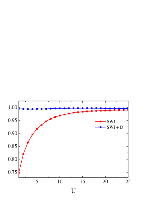
Figure 7: Spectral-weight integral [equation (19)] shown alone (red) and corrected by the average double occupancy, $D$ (blue).

4.4 Spectral-Weight Integral

We comment here that, from the properties of the Green function, the density of states of electrons with both spin orientations should obey the sum rule

$$\int_{-\infty}^{\infty}d\omega\rho(\omega)=1.$$ (18)

In our results, because one of the two bosonic operators on each sublattice undergoes Bose-Einstein condensation [equation (7)], the sum rule is violated and instead takes the form

$$\int_{-\infty}^{\infty}d\omega\rho(\omega)=1-D,$$ (19)

where $D$ is the average double-occupancy parameter calculated in section 3. In figure 7 we show both the spectral-weight integral and its value corrected by the average double occupancy, for a range of values of $U$. Because our calculation is performed using a finite energy interval, the corrected spectral-weight integral is less than 1, but it is clear that the deviations are very small for all intermediate values of $U$. In the atomic limit, $D=0$, the sum rule is satisfied by the spectral weight alone, while for finite $U$ the spectral-weight integral violates the sum rule by an amount equivalent to $D$ and approaches $1$ as $U$ increases. For an intermediate interaction strength such as $U=8$, we observe that the spectral-weight integral is $0.96$, indicating that our strong-coupling approximation remains robust, and capable of capturing the primary physics of the Hubbard model, in this regime. Only at weak coupling, where the spin-wave treatment of the Heisenberg model is not suitable, higher-order perturbations are important and charge fluctuations become strong, does the SCBA fail to reproduce the complex charge dynamics.

5 Luttinger Volume

Landau’s Fermi-liquid theory is one of the fundamental theories in quantum many-body physics. Its most important single qualitative result is that the Fermi surface still exists, even in the presence of interactions, in all dimensions higher than 1. For the normal metals that can be described as Fermi liquids, the shape of the Fermi surface is essential in determining the thermodynamic and transport properties of the system, because only electrons close to the Fermi surface can be excited at low energies. For a given electron density, regardless of the shape of the Fermi surface, the volume it encloses is invariant even when interactions between particles are taken into consideration. This result, the Luttinger theorem [93, 94, 95], relates the total electron density to the volume in momentum space where the Green function is positive,

$$\frac{N}{V}=2\int_{G(\mathbf{k},\omega=0)>0}\frac{d^{d}k}{(2\pi)^{d}},$$ (20)

with $d$ the spatial dimension of the system. Although the original proof by Luttinger was based on perturbation theory, and thus the theorem may in principle be violated by nonperturbative effects, Oshikawa [95] has provided a nonperturbative proof based on topological arguments. In essence, the insensitivity of the result to any interactions should be considered as a quantisation phenomenon [95], and therefore the Luttinger theorem may be the first example of topological quantisation discovered for the quantum many-body problem.

In general, the poles of the electron Green function, $G(\mathbf{k},\omega)$, determine the band dispersion and define the Fermi surface at the chemical potential, where $\omega=0$. From the asymptotic behaviour $G(\mathbf{k},\omega\rightarrow\infty)\propto 1/\omega$, it is obvious that the limiting Green function is positive for positive $\omega$ and conversely. For a Fermi liquid, as the frequency approaches the Fermi surface ($\omega=0$), by definition $G(\mathbf{k},\omega=0^{+})\rightarrow+\infty$ while $G(\mathbf{k},\omega=0^{-})\rightarrow-\infty$, implying that the Green function must change sign at the Fermi surface through an infinity in $G(\mathbf{k},0)$ if there are no singularities in any other regions of $\mathbf{k}$ and $\omega$. The Luttinger theorem then concerns precisely the volume enclosed by the surfaces where $G(\mathbf{k},0)$ changes sign.

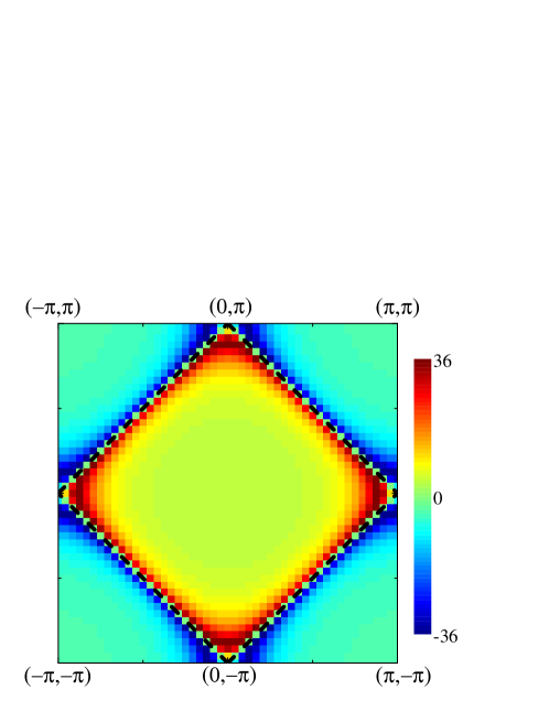
Figure 8: Real part of the inverse Green function, $\textrm{Re}[G^{-1}(\mathbf{k},\omega=0)]$, for the half-filled Hubbard model on the square lattice, calculated for $U=8$. $\textrm{Re}[G^{-1}(\mathbf{k},\omega=0)]$ changes sign from a negative to a positive maximum through a diamond-shaped boundary. The sign-change gives the Luttinger surface at $\omega=0$, and coincides with the locus of solutions of $\cos k_{x}+\cos k_{y}=0$, marked by the black, dashed line.

However, this change of sign is not always connected with an infinity. It may also occur through zeros of the Green function [24, 64, 65, 66, 67, 87], and in fact these are the relevant quantities for insulating systems, where there is no Fermi surface. By contrast, all systems have a Luttinger surface, and this may be defined from the zeros. Examples of this type of physics include the BCS superconductor, where $G(\mathbf{k},0)$ changes sign through the chemical potential in the absence of a Fermi surface, and also the Mott insulator.

For systems with a full gap spanning some energy interval (figures 4 and 5), the self-energy inside the gap must be infinite as otherwise spectral features would appear. For the Green function, the divergence of the self-energy implies (11) that $G(\mathbf{k},\omega)=0$ and thus the poles of the self-energy can be used to define the Luttinger surface. Here we use the real part of the inverse Green function to calculate the Luttinger surface, which in terms of $\textrm{Re}[G^{-1}(\mathbf{k},\omega)]$ corresponds to its points of divergence, whereas the band dispersion is given by its zeros. We note that the self-energy can have only one pole, $\xi_{k}$, in an energy regime where a gap is present; a situation with two successive poles, $\xi_{k,1}<\xi_{k,2}$, would give $\textrm{Re}[G^{-1}(\mathbf{k},\xi_{k,1}+0^{+})]\rightarrow+\infty$ and $\textrm{Re}[G^{-1}(\mathbf{k},\xi_{k,2}+0^{-})]\rightarrow-\infty$, which would require a zero of $\textrm{Re}[G^{-1}(\mathbf{k},\omega)]$ in the gap region, contradicting the definition.

In figure 8 we show the real part of the inverse Green function in the form of colour contours. The finite broadening factor, $\eta$, in our calculation converts the divergence into a sharp minimum followed by an equally sharp maximum as a function of $|\mathbf{k}|$. It is clear that $\textrm{Re}[G^{-1}(\mathbf{k},\omega=0)]$ changes sign from negative to positive through a diamond-shaped boundary, which therefore marks the zeros of the Green function at $\omega=0$, i.e. the Luttinger surface. This surface is specified precisely by the condition $\cos k_{x}+\cos k_{y}=0$, and therefore we have found that the Luttinger surface is exactly the Fermi surface of non-interacting electrons. This result is a consequence of particle-hole symmetry at half-filling. Although the system is completely gapped in the Mott-insulating phase, the Luttinger theorem remains applicable and for the half-filled Hubbard model can be interpreted as the integral of the region within the Luttinger surface [69].

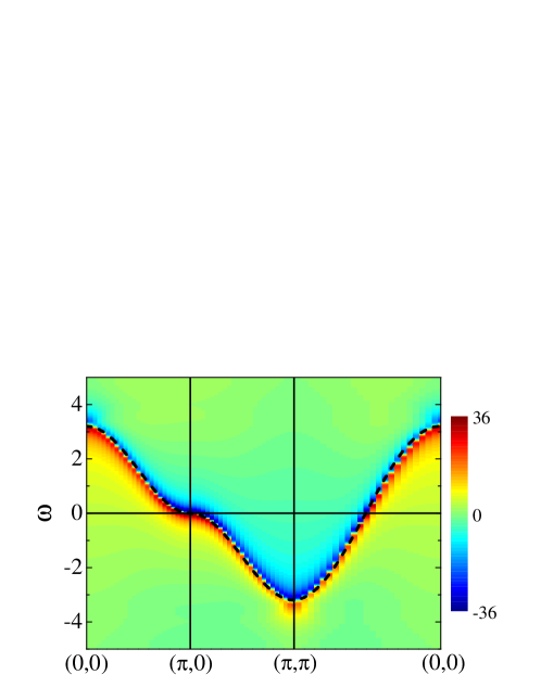
Figure 9: Real part of the inverse Green function, $\textrm{Re}[G^{-1}(\mathbf{k},\omega)]$, calculated using $U=8$ for values of $\mathbf{k}$ chosen along the high-symmetry directions. The black, dashed curve shows the function $1.6t(\cos k_{x}+\cos k_{y})$ (see text).

To gain more insight into the behaviour of the self-energy, in figure 9 we show $\textrm{Re}[G^{-1}(\mathbf{k},\omega)]$ calculated with $U=8$ for the primary high-symmetry directions in momentum space. The divergence of the inverse Green function can be regarded as a dispersion relation defined by the self-energy, and it forms a rather clear quasiparticle band. The black, dashed curve in figure 9 shows the function $2t_{\rm eff}(\cos k_{x}+\cos k_{y})$ with $t_{\rm eff}=0.8t$, which obviously provides a reasonable, if not perfect, fit to the zeros of the calculated Green function. This form, which resembles an inverted free-electron dispersion with a renormalised hopping parameter, is quite similar to the results obtained by exact diagonalisation [24], except in that the effective hopping is smaller.

To interpret this result, we note first that the inverted nature of the quasiparticle band signifies its holonic origin. From equation (33), we expect that the doublon band will have the same form as the holon band but with a momentum shift of $\mathbf{Q}$. Thus the poles of the electron self-energy are given directly by the dispersion relation of the quasiparticles, which is in turn connected with the non-interacting dispersion, $2t(\cos k_{x}+\cos k_{y})$, by a renormalisation factor. Second, from equation (47) one observes that this renormalisation of the effective quasiparticle dispersion, $4tb_{0}^{2}\gamma_{\mathbf{k}}=2tb_{0}^{2}(\cos k_{x}+\cos k_{y})$, is related directly to the holon-doublon pairing interaction term, which in turn is determined by the magnetic ordering (condensation) parameter, $b_{0}$. In the limit of large $U$, the Mott gap saturates at $\Delta=U$ (section 4.3) and, as discussed in B.1, magnetic order becomes robust, with an ordered moment of $m_{s}=0.321$ and, from equation (8), $b_{0}^{2}=0.821$ in our calculations. The effective quasiparticle hopping parameter, $t_{\rm eff}$, is shown in figure 10, which compares the results extracted from the Green function in a simple mean-field approximation, with only holon-doublon interactions but without spin-fluctuation effects, to the results of the SCBA. Also shown for comparison is the result of a direct determination of $b_{0}^{2}$, which allows us to deduce that the effective hopping parameter saturates at $t_{\rm eff}=b_{0}^{2}t=0.821t$ as $U\rightarrow\infty$ in the mean-field approximation. However, the effect of the additional spin fluctuations contained in the SCBA is to allow the effective hopping to be stronger than the value constrained by the condensation parameter.

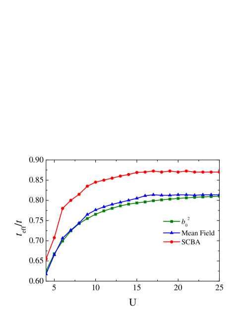
Figure 10: Effective hopping parameter, $t_{\rm eff}$, defined by the poles of the electron self-energy, $2t_{\rm eff}(\cos k_{x}+\cos k_{y})$, calculated in a mean-field approximation with no spin-fluctuation effects (blue) and in the SCBA (red); for comparison we show also the condensation parameter, $b_{0}^{2}$ (green).

Away from strong coupling, the departure of the quasiparticle mass from the high-$U$ limit may be taken as a further indication of the effects of charge and spin fluctuations at intermediate $U$, which includes the value $U=8$ shown in figure 9. The reduction of $t_{\rm eff}$ computed in the SCBA with decreasing $U$ is clear in figure 10, where again the comparison with the mean-field form and $b_{0}^{2}$ allows us to benchmark the effects of spin fluctuations and of self-consistency at intermediate $U$ within our calculation. The Mott gap is effectively the mass term, $U$, in equation (47) and its downward renormalisation with decreasing $U$ is also the consequence of holon-doublon interactions, renormalised at intermediate $U$ by spin fluctuations, as discussed in section 4 and shown in figures 4 and 5. However, this information is not visible in the inverse Green function, which therefore can be taken as a measure only of the spin-fluctuation renormalisation effect within the SCBA, independently of the Mott-gap scale.

We conclude that the holon-doublon description contains valuable insight into the static and dynamic properties of the charge degrees of freedom. The characteristic feature of the Mott insulator is not the Fermi surface but the Luttinger surface. The Luttinger theorem for the Fermi liquid holds for the half-filled Hubbard model, despite its insulating nature, with the sign-change of the Green function at $\omega=0$ caused by its zeros instead of its poles. This Luttinger surface appears inside the Mott gap, which separates the lower and upper Hubbard bands, and it defines a quasiparticle band whose renormalisation characterises the effects of spin interactions on the charge sector.

6 Optical Conductivity

The final quantity we calculate is the optical conductivity. Optical conductivity measurements [90, 91], which reveal the carrier number, the size of the energy gap, the dynamics of quasiparticle excitations and their scattering processes, have played an important role in the study of many classes of correlated electronic materials. For the insulating parent compounds of the high-$T_{c}$ superconductors, optical conductivity measurements performed on La₂CuO₄ at a temperature of $300$ K show an excitonic absorption peak at $2$ eV [96]. This behaviour was ascribed to the strongly correlated but charge-transfer-dominated character of the undoped CuO₂ plane [97]. When holes are doped into the system, optical conductivity measurements show a number of features that deviate strongly from conventional band theory. The most striking phenomenon is the reconstruction of the electronic spectral weight at low doping, which involves the transfer of weight from the charge-transfer excitation regime to a mid-infrared band, centred at approximately $0.5$ eV. This mid-infrared band is consistent with the appearance of in-gap states [86, 92] but to date there is no theory for its microscopic origin. As the doping is increased, a Drude-type response develops at far-infrared frequencies and decays much more slowly than band theory would predict. This characteristic spectral-weight transfer is evidently intrinsic to the Mott insulator and cannot be described by a theory ignoring electronic correlations. It has been argued [63, 98] that this property of the Mott phase can be explained within the Hubbard model, but there is as yet no consensus on the complete dynamics of the weight-transfer phenomenon.

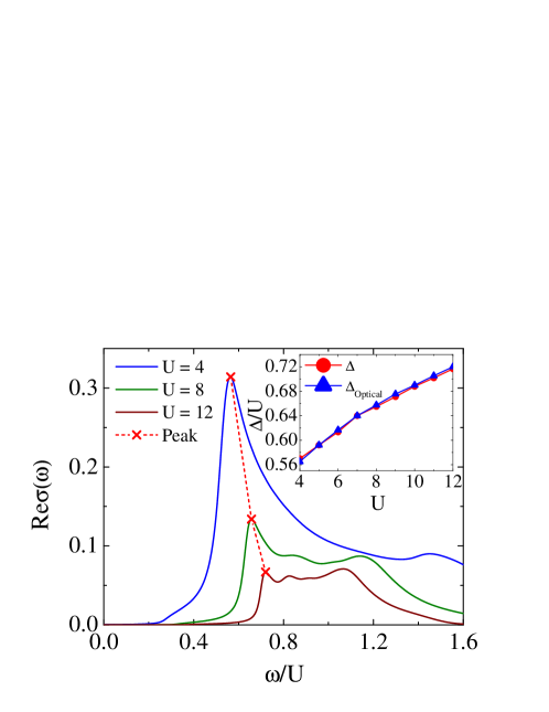
Figure 11: Real part of the optical conductivity as a function of frequency, shown for a number of $U$ values. The results were calculated on a $48\times 48$ lattice at zero temperature. The red, dashed line connects the initial peaks on each curve, which determine the optical gap, $\Delta_{\rm Optical}$. The inset compares $\Delta_{\rm Optical}$ with the Mott gap, $\Delta$, determined from the peak separation in figure 5.

The optical conductivity in the $x$ direction can be calculated from the imaginary part of the current-current correlation function,

$$\mathrm{Re}[\sigma_{xx}(\omega)]=-\mathrm{Im}\left[\frac{1}{\omega}\Pi_{xx}^{R}(\omega)\right],$$ (21)

as discussed in detail in C. The results we obtain within the slave-particle framework and the SCBA are shown in figure 11 for a number of $U$ values spanning the intermediate-coupling regime. The optical conductivity has a clear charge-excitation gap, as expected for an insulating system (but in contrast to the Drude peak predicted by conventional band theory). The first peak is expected at the “optical gap,” $\Delta_{\rm Optical}$, which is determined by a two-particle process; as $U$ increases, its location clearly moves to higher energy, even when normalised to $U$, and its peak height drops. This is consistent with experimental results for the optical reflectivity spectra [96], and with the expectation of a larger quasiparticle gap with increasing $U$ contained in figure 5. The Mott gap is the one-particle charge gap and is determined from the separation of the leading peaks in the lower and upper Hubbard bands, as shown in the spectral function [figure 4(a)] and the density of states [figure 5(b)]. The inset of figure 11 compares the Mott gap with the optical gap obtained in the main panel, and it is clear that the two are almost identical for the Mott insulator.

Exact diagonalisation results [99, 100, 23] and quantum Monte Carlo calculations [26] also confirm the insulating character of the undoped Hubbard model. The optical conductivity given by exact diagonalisation [100] shows a sharp peak at the Mott-gap edge, which is attributed to spin-polaron formation in the photoexcited state, as also revealed by DMFT [101]. Although these results suggest a separation of the spin-polaron band from the high-energy feature, we caution that the system sizes used are very small; in our calculations, the spectral function has a continuous and multipeak structure for most wavevectors $\mathbf{k}$, with no clear band separation and thus no discrete peaks in the optical conductivity. We do not attempt a quantitative comparison of our results with other numerical methods because the effect of vertex corrections [102, 104] cannot be neglected in the calculation of optical conductivity.

As a consequence of fundamental conservation laws, the optical conductivity obeys the sum rule [90, 91, 104]

$$\int_{0}^{\infty}d\omega\mathrm{Re}[\sigma_{xx}(\omega)]=-\frac{\pi}{2}\langle T_{x}\rangle,$$ (22)

where $\langle T_{x}\rangle$ is the average kinetic energy in the $x$ direction. In our calculations for the half-filled Hubbard model, the results do not satisfy this sum rule exactly, although the deviation is within $10\%$ for all intermediate $U$ values. This discrepancy is presumably caused by the spectral-weight loss discussed in section 4, as well as by our neglect of vertex corrections. The inclusion of the latter, and of higher-order physical processes, may be expected to produce superior results, and to be increasingly important for calculations at lower $U$ or at any finite temperatures.

7 Summary

We have used a holon-doublon slave-fermion representation in the self-consistent Born approximation to investigate the charge dynamics of the single-band Hubbard model at half-filling on the square lattice. We show that holon-doublon binding is intrinsic to the Mott-insulating state. As expected in a nearest-neighbour hopping model, the system is always insulating and the monotonically decreasing doublon density shows no critical value, $U_{c}$, where a metal-insulator transition occurs. The electronic density of states we compute has a coherent quasiparticle band accompanied by incoherent lower and upper Hubbard bands. The Mott gap is the excitation gap of the holons and doublons, and so is determined by their binding energy. We calculate the Luttinger surface of the Green function at the chemical potential and demonstrate that, for the Mott insulator, the Luttinger theorem can be interpreted as the integral of the region enclosed by this Luttinger surface rather than a Fermi surface. We show further that the poles of the self-energy define an effective quasiparticle dispersion similar to that of free electrons, but with a renormalised hopping parameter. The optical conductivity displays clearly both the Mott gap and the incoherent Hubbard bands.

In this slave-fermion description, the Mott-gap state is accompanied by the formation of holon-doublon bound states. Holon-doublon binding provides the energy scale of the Mott gap in the half-filled Hubbard model. In greater detail, the pairing interaction of holons and doublons is a $k$-space phenomenon, occurring across the Fermi surface. We comment that both holons and doublons are components of the quasiparticles making up the lower Hubbard band, as they are of the upper, and thus the paired state should not be considered as an exciton; indeed, holon-doublon pairs would remain present at finite doping, when the particle-hole symmetry of the half-filled system is lost. The presence of these bound states, together with the interactions between the charge carriers and the magnons, reflects the fact that the high- and low-energy degrees of freedom in the Hubbard model are intrinsically mixed, with the spin fluctuations playing an essential role in the construction of coherent “spin-polaron” features in the lower and upper Hubbard bands.

Our technique is a strong-coupling approach, valid at large values of $U$, and can be used to obtain the analytical limiting forms of all physical quantities in this regime. At intermediate $U$ values, it provides accurate results for the evolution of the charge dynamics as a consequence of the renormalising effects of spin fluctuations. Only on the approach to the weak-coupling regime do we find systematic discrepancies in the framework, which we may characterise by violations of the spectral sum rule. In this regime, the single-mode approximation to the spin dynamics of the Néel antiferromagnetic ground state begins to break down, the self-consistent Born approximation requires the inclusion of vertex corrections and even the decoupling of electron operators into separate spin and charge parts may no longer be justified. As noted in section 1, a degree of confusion exists in the literature over whether the insulating properties of the weakly coupled system can be ascribed to magnetic rather than to electrostatic interactions, and we conclude from the absence of a transition that the two pictures are different sides of the same coin, driven by the same fundamental processes. However, the slave-fermion framework adopted here is clearly not the appropriate method for investigating the crossover from the robustly Mott-insulating regime to the noninteracting limit.

Despite this deficiency far from its regime of validity, we have demonstrated that the holon-doublon representation provides both a full qualitative understanding of the underlying physics of the Mott insulator and a semi-quantitative account of its physical properties across the full range of intermediate and strong interactions. Our results for the Mott state have a transparent origin, not obscured by the complexities of a many-body numerical calculation, and indeed can be used to verify the features and parameter-dependences found in numerical studies. Although one may argue that the half-filled system at zero temperature is already fully characterised, the holon-doublon description we have introduced here provides a valuable foundation for understanding both the charge dynamics of the half-filled Hubbard model at finite temperatures and the evolution of the Mott gap as the system is doped away from half-filling.

Appendix A Hubbard Hamiltonian

A.1 Heisenberg Model

The spin degrees of freedom are assumed to be governed by the Heisenberg model, which is treated in the linear spin-wave approximation using the condensation assumption of equation (7). Despite the extreme quantum nature of the $S=1/2$ spins, a linear spin-wave treatment has been shown [53] to provide a good description of the ordered phase with only small, quantitative, and well characterised renormalisation parameters. In momentum space, the Hamiltonian can be expressed as

$$H_{S}={\textstyle\frac{1}{4}}Jzb_{0}^{2}\sum_{\mathbf{k}}(\!\begin{array}[c]{cc}s_{\mathbf{k}}^{{\dagger}}&s_{-\mathbf{k}}\end{array}\!)\left(\!\!\begin{array}[c]{cc}1&\gamma_{\mathbf{k}}\\ \gamma_{\mathbf{k}}&1\end{array}\!\!\right)\left(\!\!\begin{array}[c]{c}s_{\mathbf{k}}\\ s_{-\mathbf{k}}^{{\dagger}}\end{array}\!\!\right)+C,$$ (23)

where $C$ is a constant. The Bogoliubov transformation

$$\left(\!\!\begin{array}[c]{c}s_{\mathbf{k}}\\ s_{-\mathbf{k}}^{{\dagger}}\end{array}\!\!\right)=\left(\!\!\begin{array}[c]{cc}u_{\mathbf{k}}&v_{\mathbf{k}}\\ v_{\mathbf{k}}&u_{\mathbf{k}}\end{array}\!\!\right)\left(\!\!\begin{array}[c]{c}\alpha_{\mathbf{k}}\\ \alpha_{-\mathbf{k}}^{{\dagger}}\end{array}\!\!\right)\!,$$ (24)

with

$$u_{\mathbf{k}}^{2}=\frac{1}{2}+\frac{1}{2\omega_{\mathbf{k}}},\;v_{\mathbf{k}}^{2}=-\frac{1}{2}+\frac{1}{2\omega_{\mathbf{k}}},\;u_{\mathbf{k}}v_{\mathbf{k}}=-\frac{\gamma_{\mathbf{k}}}{2\omega_{\mathbf{k}}},\;\omega_{\mathbf{k}}=\sqrt{1-\gamma_{\mathbf{k}}^{2}}$$ (25)

and

$$\gamma_{\mathbf{k}}=\frac{1}{z}\sum_{\boldsymbol{\delta}}e^{i\mathbf{k\cdot}\boldsymbol{\delta}},$$ (26)

in which $z=4$ is the coordination number and $\boldsymbol{\delta}=(\pm a,0)$ and $(0,\pm a)$, yields the form

$$H_{S}=\sum_{\mathbf{k}}\Omega_{\mathbf{k}}(\alpha_{\mathbf{k}}^{{\dagger}}\alpha_{\mathbf{k}}+{\textstyle\frac{1}{2}}),$$ (27)

where

$$\Omega_{\mathbf{k}}={\textstyle\frac{1}{2}}Jzb_{0}^{2}\omega_{\mathbf{k}}$$ (28)

is the magnon dispersion relation. In this approximation, the energy of the magnon is reduced by the self-consistent condensation parameter $b_{0}^{2}$, reflecting the renormalisation of the effective Heisenberg coupling constant caused by the on-site interaction, $U$.

The two types of magnon Green function are defined by

$$D_{1}\left(\mathbf{q},\tau\right) =-\left\langle T_{\tau}\alpha_{\mathbf{q}}\left(\tau\right)\alpha_{\mathbf{q}}^{{\dagger}}\left(0\right)\right\rangle\!,$$

$$D_{2}\left(\mathbf{q},\tau\right) =-\left\langle T_{\tau}\alpha_{\mathbf{q}}^{{\dagger}}\left(\tau\right)\alpha_{\mathbf{q}}\left(0\right)\right\rangle\!,$$ (29)

and their Fourier transforms are

$$D_{1}\left(\mathbf{q},i\omega_{n}\right)=\frac{1}{i\omega_{n}-\Omega_{\mathbf{q}}},\;\;D_{2}\left(\mathbf{q},i\omega_{n}\right)=-\frac{1}{i\omega_{n}+\Omega_{\mathbf{q}}}.$$ (30)

In figure 1, $\mathbf{D}$ is a $2\times 2$ matrix whose explicit form is

$$\mathbf{D}_{11} =g_{1}^{2}\left(\mathbf{k,q}\right)D_{1}+g_{2}^{2}\left(\mathbf{k,q}\right)D_{2},$$

$$\mathbf{D}_{12} =-g_{1}\left(\mathbf{k,q}\right)g_{2}\left(\mathbf{k,q}\right)[D_{1}+D_{2}],$$

$$\mathbf{D}_{21} =-g_{1}\left(\mathbf{k,q}\right)g_{2}\left(\mathbf{k,q}\right)[D_{1}+D_{2}],$$

$$\mathbf{D}_{22} =g_{2}^{2}\left(\mathbf{k,q}\right)D_{1}+g_{1}^{2}\left(\mathbf{k,q}\right)D_{2},$$ (31)

where

$$g_{1}(\mathbf{k,q}) ={\textstyle\frac{1}{\sqrt{N}}}tb_{0}z(u_{q}\gamma_{q-k}+v_{q}\gamma_{k}),$$

$$g_{2}(\mathbf{k,q}) ={\textstyle\frac{1}{\sqrt{N}}}tb_{0}z(u_{q}\gamma_{k}+v_{q}\gamma_{k-q}).$$ (32)

A.2 Hubbard model

Within the same condensation approximation, the full Hubbard Hamiltonian (4) is given by

$$H ={\textstyle\frac{1}{2}}U\sum_{\mathbf{k}}(d_{\mathbf{k}}^{\dagger}d_{\mathbf{k}}+e_{\mathbf{k}}^{\dagger}e_{\mathbf{k}})$$ (33)

$$\quad+4tb_{0}^{2}\sum_{\mathbf{k}}(d_{\mathbf{Q}-\mathbf{k}}^{\dagger}e_{\mathbf{k}}^{\dagger}\gamma_{\mathbf{k}}+e_{\mathbf{k}}d_{\mathbf{Q}-\mathbf{k}}\gamma_{\mathbf{k}})$$

$$\quad-\frac{tb_{0}z}{\sqrt{N}}\sum_{\mathbf{k},\mathbf{q}}d_{\mathbf{k}}^{\dagger}d_{\mathbf{k-q}}(\gamma_{\mathbf{k}}s_{-\mathbf{q}}^{\dagger}+\gamma_{\mathbf{k}-\mathbf{q}}s_{\mathbf{q}})$$

$$\quad+\frac{tb_{0}z}{\sqrt{N}}\sum_{\mathbf{k},\mathbf{q}}e_{\mathbf{k}}^{\dagger}e_{\mathbf{k}-\mathbf{q}}(\gamma_{\mathbf{k}}s_{-\mathbf{q}}^{\dagger}+\gamma_{\mathbf{k}-\mathbf{q}}s_{\mathbf{q}}).$$

The first line expresses a mass term for the holons and doublons, whose pairing interaction, in the second line, gives them a dispersive kinetic term in the unperturbed charge Green function. The factor of $b_{0}^{2}$ contains the renormalisation of the pairing strength due to spin fluctuations. The third and fourth lines of equation (33) express the fact that the hopping of holons and doublons is coupled with the emission and absorption of magnons, and we treat this three-body scattering interaction by the SCBA.

In terms of the Nambu spinor, $\psi_{\mathbf{k}}^{\dagger}=(\!\!\begin{array}[c]{cc}d_{-\mathbf{k}+\mathbf{Q}}^{\dagger}&e_{\mathbf{k}}\end{array}\!\!)$, the Hamiltonian takes the matrix form

$$H=H_{C}+H_{CS},$$ (34)

in which

$$H_{C}=\sum_{\mathbf{k}}\psi_{\mathbf{k}}^{\dagger}\tilde{\varepsilon}_{\mathbf{k}}\psi_{\mathbf{k}}$$ (35)

describes the charge dynamics, contained in the first two lines of equation (33), while the interaction between the charge and spin degrees of freedom (latter two lines) is given by

$$H_{CS}=\sum_{\mathbf{k},\mathbf{q}}\psi_{\mathbf{k}}^{\dagger}M(\mathbf{k},\mathbf{q})\psi_{\mathbf{k}-\mathbf{q}};$$ (36)

in equations (35) and (36) we have defined

$$\tilde{\varepsilon}_{\mathbf{k}}=\left(\!\!\begin{array}[c]{cc}U/2&4tb_{0}^{2}\gamma_{\mathbf{k}}\\ 4tb_{0}^{2}\gamma_{\mathbf{k}}&-U/2\end{array}\!\!\right)\!\!,$$ (39)

$$M(\mathbf{k},\mathbf{q})=\left(\!\!\begin{array}[c]{cc}M_{11}(\mathbf{k},\mathbf{q})&0\\ 0&M_{22}(\mathbf{k},\mathbf{q})\end{array}\!\!\right)\!\!,$$ (42)

$$M_{11}(\mathbf{k},\mathbf{q})=g_{2}(\mathbf{k,q})\alpha_{\mathbf{q}}^{{\dagger}}+g_{1}(\mathbf{k,q})\alpha_{-\mathbf{q}},$$

$$M_{22}(\mathbf{k},\mathbf{q})=-g_{1}(\mathbf{k,q})\alpha_{\mathbf{q}}^{{\dagger}}-g_{2}(\mathbf{k,q})\alpha_{-\mathbf{q}}.$$

The unperturbed charge Green function is given by

$$\mathbf{F}^{(0)}(\mathbf{k},i\omega_{n}) =[i\omega_{n}-\tilde{\varepsilon}_{\mathbf{k}}]^{-1}$$ (43)

$$=\frac{1}{(i\omega_{n}-E_{\mathbf{k}})(i\omega_{n}+E_{\mathbf{k}})}\left(\!\!\begin{array}[c]{cc}i\omega_{n}+U/2&4tb_{0}^{2}\gamma_{\mathbf{k}}\\ 4tb_{0}^{2}\gamma_{\mathbf{k}}&i\omega_{n}-U/2\end{array}\!\!\right)\!\!,$$ (46)

where

$$E_{\mathbf{k}}=\sqrt{{\textstyle\frac{1}{4}}U^{2}+(4tb_{0}^{2}\gamma_{\mathbf{k}})^{2}}$$ (47)

is the quasiparticle dispersion relation for the charge degrees of freedom.

The self-consistent Dyson equation for the full Green function in the presence of spin-fluctuation interactions is calculated in the SCBA to deduce the Green function,

$$\mathbf{F}(\mathbf{k},i\omega_{n})=\frac{1}{i\omega_{n}-\tilde{\varepsilon}_{\mathbf{k}}-\mathbf{\Sigma}(\mathbf{k},i\omega_{n})},$$ (48)

of equation (11) with the self-energy given by

$$\mathbf{\Sigma}(\mathbf{k},i\omega_{n}) =\sum_{\mathbf{q}}\int_{-\infty}^{\infty}d\varepsilon\frac{1-f(\varepsilon)}{i\omega_{n}-\varepsilon-\Omega_{\mathbf{q}}}\mathbf{g}(\mathbf{k,q})\mathbf{A}_{1}(\mathbf{k}-\mathbf{q},\varepsilon)\mathbf{g}(\mathbf{k,q})$$ (49)

$$+\sum_{\mathbf{q}}\int_{-\infty}^{\infty}d\varepsilon\frac{f(\varepsilon)}{i\omega_{n}-\varepsilon+\Omega_{\mathbf{q}}}\mathbf{g}(\mathbf{k,q})\mathbf{A}_{2}(\mathbf{k}-\mathbf{q},\varepsilon)\mathbf{g}(\mathbf{k,q}),$$

in which

$$\mathbf{g}(\mathbf{k,q})=\left[\begin{array}[c]{cc}g_{1}(\mathbf{k,q})&0\\ 0&-g_{2}(\mathbf{k,q})\end{array}\right]\!\!,$$ (50)

and

$$\mathbf{A}_{1}(\mathbf{k},\varepsilon) = \left[\begin{array}[c]{cc}A_{11}(\mathbf{k},\varepsilon)&A_{12}(\mathbf{k},\varepsilon)\\ A_{21}(\mathbf{k},\varepsilon)&A_{22}(\mathbf{k},\varepsilon)\end{array}\right]\!\!,$$ (53)

$$\mathbf{A}_{2}(\mathbf{k},\varepsilon) = \left[\begin{array}[c]{cc}A_{22}(\mathbf{k},\varepsilon)&A_{12}(\mathbf{k},\varepsilon)\\ A_{21}(\mathbf{k},\varepsilon)&A_{11}(\mathbf{k},\varepsilon)\end{array}\right]\!\!,$$ (56)

with

$$A_{\alpha\beta}(\mathbf{k},\varepsilon)=-\frac{1}{\pi}\rm{I}\rm{m}F_{\alpha\beta}^{R}(\mathbf{k},\varepsilon+i\eta)$$ (57)

the spectral function corresponding to the retarded Green function and $f(\varepsilon)$ the Fermi distribution function.

Appendix B Large-$U$ Limit

Because the slave-fermion treatment of the Hubbard model is exact in the limit of strong on-site Coulomb repulsion, the SCBA affords valuable insight both into the limiting properties and into the effects of charge and spin fluctuations away from the limiting regime. In this appendix we review the magnetic order, Green function and approximate spectral properties at large $U$.

B.1 Bose Condensation and Magnetic Order

In the slave-fermion decomposition, the self-consistent condition has the form [equation (8)]

$$\frac{1}{N}\sum_{\mathbf{k}}\left[\langle d_{\mathbf{k}}^{\dagger}d_{\mathbf{k}}\rangle+\langle e_{\mathbf{k}}^{\dagger}e_{\mathbf{k}}\rangle+v_{\mathbf{k}}^{2}\right]+b_{0}^{2}=1,$$ (58)

where the coefficient $v_{\mathbf{k}}^{2}$ of the Bogoliubov transformation is defined in equation (25). At half-filling and in the large-$U$ limit, $\sum_{\mathbf{k}}\langle d_{\mathbf{k}}^{\dagger}d_{\mathbf{k}}\rangle=\sum_{\mathbf{k}}\langle e_{\mathbf{k}}^{\dagger}e_{\mathbf{k}}\rangle=0$, leaving

$$b_{0}^{2}=1-\frac{1}{N}\sum_{\mathbf{k}}v_{\mathbf{k}}^{2}\simeq 0.803$$ (59)

for the nearest-neighbour kinetic term.

In the Schwinger-boson representation, the staggered magnetisation of the magnetically ordered phase is related to this condensed fraction by

$$m_{s} = \frac{1}{N}\sum_{i}\langle S_{i}^{z}\rangle=\frac{1}{N}\sum_{i}\frac{1}{2}(\langle s_{i,\uparrow}^{{\dagger}}s_{i,\uparrow}\rangle-\langle s_{i,\downarrow}^{{\dagger}}s_{i,\downarrow}\rangle)$$ (60)

$$= \frac{1}{2}b_{0}^{2}-\frac{1}{2N}\sum_{\mathbf{k}}v_{\mathbf{k}}^{2}\simeq 0.303.$$

One observes that this treatment of the $S=1/2$ system yields a remarkably accurate reproduction of the known ordered moment, $m_{s}\simeq 0.306$, computed by unbiased numerical methods [103]. Our calculations are performed on a square lattice of size $48\times 48$ sites with periodic boundary conditions, and due to this finite-size effect give the approximate values

$$b_{0}^{2}\simeq 0.821,\;\;\;\;m_{s}\simeq 0.321.$$ (61)

B.2 Green Function and Double Occupancy

In the strong-coupling limit, to lowest order one may consider only the charge part of the Hamiltonian, $H_{C}$ in equation (34), and neglect the terms $H_{CS}$ describing the interaction of the charge degrees of freedom with the spin fluctuations. In this approximation, the doublon Green function

$$\mathbf{F}_{11}^{(0)}(\mathbf{k},\tau)=-\left\langle T_{\tau}\left[d_{-\mathbf{k}+\mathbf{Q}}(\tau)d_{-\mathbf{k}+\mathbf{Q}}^{\dagger}(0)\right]\right\rangle\!,$$ (62)

may be expressed as

$$\mathbf{F}_{11}^{(0)}(\mathbf{k},i\omega_{n})=\frac{i\omega_{n}+U/2}{(i\omega_{n}-E_{\mathbf{k}})(i\omega_{n}+E_{\mathbf{k}})},$$ (63)

with $E_{\mathbf{k}}$ given in equation (47).

By rewriting equation (63) in the form

$$\mathbf{F}_{11}^{(0)}(\mathbf{k},\omega+i\delta) = \frac{E_{\mathbf{k}}+U/2}{2E_{\mathbf{k}}}\frac{1}{\omega+i\delta-E_{\mathbf{k}}}+\,\frac{E_{\mathbf{k}}-U/2}{2E_{\mathbf{k}}}\frac{1}{\omega+i\delta+E_{\mathbf{k}}},$$ (64)

one obtains the spectral function

$$\mathbf{A}_{11}^{(0)}(\mathbf{k},\omega) = \frac{E_{\mathbf{k}}+U/2}{2E_{\mathbf{k}}}\delta(\omega-E_{\mathbf{k}})+\,\frac{E_{\mathbf{k}}-U/2}{2E_{\mathbf{k}}}\delta(\omega+E_{\mathbf{k}})$$ (65)

and thus the zero-temperature doublon occupation function

$$\langle d_{-\mathbf{k}+\mathbf{Q}}^{\dagger}d_{-\mathbf{k}+\mathbf{Q}}\rangle=\int_{-\infty}^{\infty}\!\!d\omega f(\omega)A_{11}^{(0)}(\mathbf{k},\omega)=\frac{E_{\mathbf{k}}-\frac{U}{2}}{2E_{\mathbf{k}}}.$$ (66)

By Taylor expansion of this expression,

$$\langle d_{-\mathbf{k}+\mathbf{Q}}^{\dagger}d_{-\mathbf{k}+\mathbf{Q}}\rangle \simeq \frac{1}{U}\left\{\frac{U}{2}\left[1+\frac{1}{2}\frac{4}{U^{2}}(4tb_{0}^{2}\gamma_{\mathbf{k}})^{2}\right]-\frac{U}{2}\right\}$$ (67)

$$\simeq (4tb_{0}^{2}\gamma_{\mathbf{k}})^{2}\frac{1}{U^{2}}$$

and the net doublon occupation is

$$D\simeq\frac{1}{U^{2}}\frac{1}{N}\sum_{\mathbf{k}}(4tb_{0}^{2}\gamma_{\mathbf{k}})^{2}\simeq\frac{2.70}{U^{2}},$$ (68)

showing asymptotic $1/U^{2}$ scaling in the large-$U$ limit.

B.3 Mott Gap

In the limit of large $U$, one may assume that the strongest contributions to the renormalisation of the Mott gap are obtained at first order in the SCBA, with higher-order contributions being heavily suppressed. In this case it is safe to assume that the off-diagonal Green-function components, $\mathbf{F}_{12}$ and $\mathbf{F}_{21}$ in equation (48), may be neglected in computing the self-energy corrections determining the Mott gap. From the doublon spectral function of equation (65) and its holon counterpart

$$\mathbf{A}_{22}^{(0)}(\mathbf{k},\omega) = \frac{E_{\mathbf{k}}-U/2}{2E_{\mathbf{k}}}\delta(\omega-E_{\mathbf{k}})+\,\frac{E_{\mathbf{k}}+U/2}{2E_{\mathbf{k}}}\delta(\omega+E_{\mathbf{k}}),$$ (69)

the self-energy components [equation (49)] calculated in the SCBA are

$$\mathbf{\Sigma}_{11}(\mathbf{k},i\omega_{n}) = \sum_{\mathbf{q}}g_{1}^{2}(\mathbf{k,q})\int_{0}^{\infty}d\varepsilon\frac{A_{11}^{(0)}(\mathbf{k}-\mathbf{q},\varepsilon)}{i\omega_{n}-\Omega_{\mathbf{q}}-\varepsilon}[1-f(\varepsilon)]$$ (70)

$$+\sum_{\mathbf{q}}g_{2}^{2}(\mathbf{k,q})\int_{-\infty}^{0}d\varepsilon\frac{A_{11}^{(0)}(\mathbf{k}-\mathbf{q},\varepsilon)}{i\omega_{n}+\Omega_{\mathbf{q}}-\varepsilon}f(\varepsilon)$$

$$= \sum_{\mathbf{q}}\frac{E_{\mathbf{k}-\mathbf{q}}+U/2}{2E_{\mathbf{k}-\mathbf{q}}}g_{1}^{2}(\mathbf{k,q})\frac{1}{i\omega_{n}-\Omega_{q}-E_{\mathbf{k}-\mathbf{q}}}$$

$$+\sum_{\mathbf{q}}\frac{E_{\mathbf{k}-\mathbf{q}}-U/2}{2E_{\mathbf{k}-\mathbf{q}}}g_{2}^{2}(\mathbf{k,q})\frac{1}{i\omega_{n}+\Omega_{q}+E_{\mathbf{k}-\mathbf{q}}}$$

$$\approx \sum_{\mathbf{q}}g_{1}^{2}(\mathbf{k,q})\frac{1}{i\omega_{n}-U/2}\;=\;\frac{a_{\mathbf{k}}}{i\omega_{n}-U/2},$$

and

$$\mathbf{\Sigma}_{22}(\mathbf{k},i\omega_{n}) = \sum_{\mathbf{q}}g_{2}^{2}(\mathbf{k,q})\int_{0}^{\infty}d\varepsilon\frac{A_{22}^{(0)}(\mathbf{k}-\mathbf{q},\varepsilon)}{i\omega_{n}-\Omega_{q}-\varepsilon}[1-f(\varepsilon)]$$ (71)

$$+\sum_{\mathbf{q}}g_{1}^{2}(\mathbf{k,q})\int_{-\infty}^{0}d\varepsilon\frac{A_{22}^{(0)}(\mathbf{k}-\mathbf{q},\varepsilon)}{i\omega_{n}+\Omega_{q}-\varepsilon}f(\varepsilon)$$

$$= \sum_{\mathbf{q}}\frac{E_{\mathbf{k}-\mathbf{q}}-U/2}{2E_{\mathbf{k}-\mathbf{q}}}g_{2}^{2}(\mathbf{k,q})\frac{1}{i\omega_{n}-\Omega_{q}-E_{\mathbf{k}-\mathbf{q}}}$$

$$+\sum_{\mathbf{q}}\frac{E_{\mathbf{k}-\mathbf{q}}+U/2}{2E_{\mathbf{k}-\mathbf{q}}}g_{1}^{2}(\mathbf{k,q})\frac{1}{i\omega_{n}+\Omega_{q}+E_{\mathbf{k}-\mathbf{q}}}$$

$$\approx \sum_{\mathbf{q}}g_{1}^{2}(\mathbf{k,q})\frac{1}{i\omega_{n}+U/2}\;=\;\frac{a_{\mathbf{k}}}{i\omega_{n}+U/2},$$

where

$$a_{\mathbf{k}}=\sum_{\mathbf{q}}g_{1}^{2}(\mathbf{k,q}).$$ (72)

The SCBA Green function [equations (46) and (48)] is then

$$\mathbf{F}(\mathbf{k},i\omega_{n})=\left[\begin{array}[]{cc}i\omega_{n}-U/2-\frac{a_{\mathbf{k}}}{i\omega_{n}-U/2}&-4tb_{0}^{2}\gamma_{\mathbf{k}}\\ -4tb_{0}^{2}\gamma_{\mathbf{k}}&i\omega_{n}+U/2-\frac{a_{\mathbf{k}}}{i\omega_{n}+U/2}\!\end{array}\right]^{\!-1}\!,$$

whose doublon and holon components are

$$\mathbf{F}_{11}(\mathbf{k},i\omega_{n})=\frac{i\omega_{n}+U/2-\frac{a_{\mathbf{k}}}{i\omega_{n}+U/2}}{\left[i\omega_{n}-U/2-\frac{a_{\mathbf{k}}}{i\omega_{n}-U/2}\right]\!\left[i\omega_{n}+U/2-\frac{a_{\mathbf{k}}}{i\omega_{n}+U/2}\right]-(4tb_{0}^{2}\gamma_{\mathbf{k}})^{2}},$$ (73)

$$\mathbf{F}_{22}(\mathbf{k},i\omega_{n})=\frac{i\omega_{n}-U/2-\frac{a_{\mathbf{k}}}{i\omega_{n}+U/2}}{\left[i\omega_{n}-U/2-\frac{a_{\mathbf{k}}}{i\omega_{n}-U/2}\right]\!\left[i\omega_{n}+U/2-\frac{a_{\mathbf{k}}}{i\omega_{n}+U/2}\right]-(4tb_{0}^{2}\gamma_{\mathbf{k}})^{2}}.$$ (74)

These functions both have four poles, which are the same in both cases,

$$E_{k}^{m}=\pm\frac{1}{2}\sqrt{4a_{\mathbf{k}}+2b_{\mathbf{k}}+U^{2}\pm 2\sqrt{4a_{\mathbf{k}}b_{\mathbf{k}}+b_{\mathbf{k}}^{2}+4a_{\mathbf{k}}U^{2}}},$$ (75)

where we have defined $b_{\mathbf{k}}=(4tb_{0}^{2}\gamma_{\mathbf{k}})^{2}$. Thus the holon and doublon gaps are both given by

$$\Delta_{e,\mathbf{k}}=\Delta_{d,\mathbf{k}}\approx U-2\sqrt{a_{\mathbf{k}}}$$ (76)

in the limit of large $U$.

The electron Green function is the convolution of the holon and doublon Green functions, which include the magnon renormalisation effects, and hence the Mott gap is given by the holon and doublon gaps. From figure 4(a), it is clear that the minimum value of this gap corresponds to the high density of states giving the clear peaks in figure 5(b). Thus by setting $\mathbf{k}=(\pi/2,\pi/2)$ and performing the $\mathbf{q}$-sum over the Brillouin zone within $a_{\mathbf{k}}$ (72) we obtain (main text)

$$\Delta={\rm min}|_{\mathbf{k}}\left[U-2\sqrt{a_{\mathbf{k}}}\right]\;=\;U-3.77$$ (77)

in the strong-coupling limit. We conclude that the approach of the Mott gap, $\Delta/U=1-3.77/U$, to unity due to the suppression of spin fluctuations in this regime is proportional to $1/U$. Because this derivation considers only the first order in the self-consistent renormalisation scheme, one may expect the coefficient to be larger than $3.77$ if higher-order processes are included.

Appendix C Optical conductivity

The conductivity tensor $\sigma_{\mu\nu}(\mathbf{q},\omega)$ is defined as the linear response of the charge current density in a solid to the total electric field,

$$\left\langle\mathcal{\hat{J}}_{\mu}(\mathbf{q},\omega)\right\rangle=\sum_{\nu}\sigma_{\mu\nu}(\mathbf{q},\omega)E_{\nu}(\mathbf{q},\omega),$$ (78)

where $\mu$ and $\nu$ denote Cartesian coordinates and $\left\langle\mathcal{\dots}\right\rangle$ denotes the equilibrium average; we use units where $e=1$, $\hbar=1$ and $c=1$. The long-wavelength $(\mathbf{q}=0)$ limit of the real part, Re$[\sigma_{\mu\nu}(\omega)]$, is referred to as the optical conductivity, because the wavelength of electromagnetic waves far exceeds the characteristic length scales of condensed matter systems, so here we derive this limit.

For a lattice system, the hopping parameter in the presence of an electromagnetic field is expressed by the Peierls substitution [104] as

$$t_{ij}=t_{ij}^{0}\rm{e}\rm{x}\rm{p}\left[i\int_{i}^{j}d\mathbf{l}\cdot\mathbf{A}(\mathbf{r},t)\right]\!\!,$$ (79)

where $\int_{i}^{j}d\mathbf{l}\cdot\mathbf{A}(\mathbf{r},t)$ is the integral of the vector potential along the hopping path. For a spatially uniform electric field, the vector potential can be taken as independent of position, $\mathbf{A}(\mathbf{r},t)\rightarrow\mathbf{A}(t)$. By restricting to the linear-response regime, expanding the phase factors to second order in $\mathbf{A}(t)$ and taking the Fourier transform, one obtains the current operator in the form

$$\mathcal{\hat{J}}_{\mu}(\mathbf{k},t)=\mathcal{\hat{J}}_{\mu}^{(1)}(\mathbf{k},t)+\mathcal{\hat{J}}_{\mu}^{(2)}(\mathbf{k},t),$$ (80)

where

$$\mathcal{\hat{J}}_{\mu}^{(1)}(\mathbf{q},t)=-\sum_{\mathbf{k},\sigma}\frac{\partial\varepsilon_{(2\mathbf{k+q})/2}}{\partial k_{x}}c_{\mathbf{k},\sigma}^{{\dagger}}c_{\mathbf{k+q},\sigma},$$ (81)

$$\mathcal{\hat{J}}_{\mu}^{(2)}(\mathbf{q},t)=-\sum_{\mathbf{k},\mathbf{p},\sigma}\frac{\partial^{2}\varepsilon_{(\mathbf{k+p})/2}}{\partial k_{x}^{2}}c_{\mathbf{k},\sigma}^{{\dagger}}c_{\mathbf{p},\sigma}A_{\mathbf{k-p}+\mathbf{q}}^{\mu}(t),$$ (82)

with $\varepsilon_{\mathbf{k}}$ the electron dispersion relation.

$\mathcal{\hat{J}}_{\mu}^{(1)}(\mathbf{k},t)$ is known as the paramagnetic current and $\mathcal{\hat{J}}_{\mu}^{(2)}(\mathbf{k},t)$ as the diamagnetic one. The latter is already linear with respect to the applied field but for the former the Kubo formula is required. To linear order in the applied field, the interaction term in the Hamiltonian is given by

$$H^{\prime}(t)=-\frac{1}{i\omega}\sum_{\mathbf{q}}\mathcal{\hat{J}}_{\mu}^{(1)}(-\mathbf{q})\mathbf{E}_{\mathbf{q}}^{\mu}e^{-i\omega t}.$$ (83)

The imaginary-time current-current correlation function is defined as

$$\Pi_{\alpha\beta}(\mathbf{q},\tau)=-\frac{1}{N}\left\langle T_{\tau}\left[\mathcal{\hat{J}}_{\alpha}^{(1)}(\mathbf{q},\tau)\mathcal{\hat{J}}_{\beta}^{(1)}(-\mathbf{q},0)\right]\right\rangle$$ (84)

and its Fourier transform as

$$\Pi_{\alpha\beta}(\mathbf{q},i\omega_{n})=\int_{0}^{\beta}d\tau e^{i\omega_{n}\tau}\Pi_{\alpha\beta}(\mathbf{q},\tau),$$ (85)

both of which are obtained from the charge Green function of equation (48). Finally, the conductivity in the $x$ direction is given by

$$\sigma_{xx}(\mathbf{q},\omega)=\frac{i}{\omega}\left[\Pi_{xx}^{R}(\mathbf{q},\omega)+\frac{1}{N}\sum_{\mathbf{k},\sigma}\frac{\partial^{2}\varepsilon_{\mathbf{k}}}{\partial k_{x}^{2}}\langle c_{\mathbf{k},\sigma}^{{\dagger}}c_{\mathbf{k},\sigma}\rangle\right]\!\!,$$ (86)

whence the real part of the optical conductivity in the limit $\mathbf{q}=0$ is

$$\mathrm{Re}[\sigma_{xx}(\omega)]=-\mathrm{Im}\left[\frac{1}{\omega}\Pi_{xx}^{R}(\omega)\right]\!\!.$$ (87)

References

References

- [1] Imada M, Fujimori A and Tokura Y 1998 Rev. Mod. Phys. 70, 1039
- [2] de Boer J H and Verwey E J W 1937 Proc. Phys. Soc. London 49, 59
- [3] Mott N F and Peierls R 1937 Proc. Phys. Soc. London 49, 72
- [4] Mott N F 1949 Proc. Phys. Soc. London, Sect. A 62, 416
- [5] Mott N F 1956 Can. J. Phys 34, 1356
- [6] Bednorz J G and Müller K A 1986 Z. Phys. B: Condens. Matter 64, 189
- [7] Hubbard J 1963 Proc. Roy. Soc. London, Ser. A 276, 238
- [8] Lieb E H and Wu F Y 1968 Phys. Rev. Lett. 20, 1445
- [9] Metzner W and Vollhardt D 1989 Phys. Rev. Lett. 62, 324
- [10] Georges A, Kotliar G, Krauth W and Rozenberg M J 1996 Rev. Mod. Phys. 68, 13
- [11] Hubbard J 1964 Proc. Roy. Soc. London, Ser. A 277, 237
- [12] Hubbard J 1964 Proc. Roy. Soc. London, Ser. A 281, 401
- [13] Hubbard J 1965 Proc. Roy. Soc. London, Ser. A 285, 542
- [14] Hubbard J 1967 Proc. Roy. Soc. London, Ser. A 296, 82
- [15] Brinkman W F and Rice T M 1970 Phys. Rev. B 2, 4302
- [16] Gutzwiller M C 1965 Phys. Rev. 137, A1726
- [17] Hirsch J E 1985 Phys. Rev. B 31, 4403
- [18] White S R, Scalapino D J, Sugar R L, Loh E Y, Gubernatis J E and Scalettar R T 1989 Phys. Rev. B 40, 506
- [19] Raghu S, Kivelson S A and Scalapino D J 2010 Phys. Rev. B 81, 224505
- [20] Dagotto E, Ortolani F and Scalapino D J 1992 Phys. Rev. B 46, 3183
- [21] Feng G S and White S R 1992 Phys. Rev. B 46, 8691(R)
- [22] Leung P W, Liu Z P, Manousakis E, Novotny M A and Oppenheimer P E 1992 Phys. Rev. B 46, 11779
- [23] Dagotto E 1994 Rev. Mod. Phys. 66, 763
- [24] Eder R, Seki K and Ohta Y 2011 Phys. Rev. B 83, 205137
- [25] White S R 1991 Phys. Rev. B 44, 4670
- [26] Bulut N, Scalapino D J and White S R 1994 Phys. Rev. Lett. 73, 748
- [27] Preuss R, Hanke W and von der Linden W 1995 Phys. Rev. Lett. 75, 1344
- [28] Gröber C, Eder R and Hanke W 2000 Phys. Rev. B 62, 4336
- [29] Varney C N, Lee C R, Bai Z J, Chiesa S, Jarrell M and Scalettar R T 2009 Phys. Rev. B 80, 075116
- [30] Baeriswyl D, Eichenberger D and Menteshashvili M 2009 New J. Phys. 11, 075010
- [31] Yanagisawa T 2013 New J. Phys. 15, 033012
- [32] Vitali E, Shi H, Qin M P and Zhang S W 2016 unpublished (arXiv:1606.04785)
- [33] Sénéchal D, Perez D and Pioro-Ladrière M 2000 Phys. Rev. Lett. 84, 522
- [34] Sénéchal D, Perez D and Plouffe D 2002 Phys. Rev. B 66, 075129
- [35] Sénéchal D and Tremblay A M S 2004 Phys. Rev. Lett. 92, 126401
- [36] Kohno M 2012 Phys. Rev. Lett. 108, 076401
- [37] Kohno M 2014 Phys. Rev. B 90, 035111
- [38] Wang Y, Wohlfeld K, Moritz B, Jia C J, van Veenendaal M, Wu K, Chen C C and Devereaux T P 2015 Phys. Rev. B 92, 075119
- [39] Potthoff M, Aichhorn M and Dahnken C 2003 Phys. Rev. Lett. 91, 206402
- [40] Dahnken C, Aichhorn M, Hanke W, Arrigoni E and Potthoff M 2004 Phys. Rev. B 70, 245110
- [41] Sénéchal D, Lavertu P L, Marois M A and Tremblay A M S 2005 Phys. Rev. Lett. 94, 156404
- [42] Aichhorn M, Arrigoni E, Huang Z B and Hanke W 2007 Phys. Rev. Lett. 99, 257002
- [43] Schäfer T, Geles F, Rost D, Rohringer G, Arrigoni E, Held K, Blümer N, Aichhorn M and Toschi A 2015 Phys. Rev. B 91, 125109
- [44] Kotliar G, Savrasov S Y, Pálsson G and Biroli G 2001 Phys. Rev. Lett. 87, 186401
- [45] Stanescu T D, Civelli M, Haule K and Kotliar G 2006 Ann. Phys. (N.Y.) 321, 1682
- [46] Park H, Haule K and Kotliar G 2008 Phys. Rev. Lett. 101, 186403
- [47] Gull E, Millis A J, Lichtenstein A I, Rubtsov A N, Troyer M and Werner P 2011 Rev. Mod. Phys. 83, 349
- [48] Sentef M, Werner P, Gull E and Kampf A P 2011 Phys. Rev. Lett. 107, 126401
- [49] Sordi G, Sémon P, Haule K, and Tremblay A M S 2012 Phys. Rev. Lett. 108, 216401
- [50] LeBlanc J P F et al 2015 Phys. Rev. X 5, 041041
- [51] Corboz P 2016 Phys. Rev. B 93, 045116
- [52] Anderson P W 1997 Adv. Phys. 46, 3
- [53] Auerbach A 1994 Interacting Electrons and Quantum Magnetism (Springer-Verlag, New York)
- [54] Castellani C, Di Castro C, Feinberg D and Ranninger J 1979 Phys. Rev. Lett. 43, 1957
- [55] Kaplan T A, Horsch P and Fulde P 1982 Phys. Rev. Lett. 49, 889
- [56] Capello M, Becca F, Fabrizio M, Sorella S and Tosatti E 2005 Phys. Rev. Lett. 94, 026406
- [57] Capello M, Becca F, Yunoki S and Sorella S 2006 Phys. Rev. B 73, 245116
- [58] Yokoyama H, Ogata M and Tanaka Y 2006 J. Phys. Soc. Jpn. 75, 114706
- [59] Miyagawa T and Yokoyama H 2011 J. Phys. Soc. Jpn. 80, 084705
- [60] Miyagawa T and Yokoyama H 2011 Physica C 471, 738
- [61] Leigh R G, Phillips P and Choy T P 2007 Phys. Rev. Lett. 99, 046404
- [62] Leigh R G and Phillips P 2009 Phys. Rev. B 79, 245120
- [63] Phillips P 2010 Rev. Mod. Phys. 82, 1719
- [64] Dzyaloshinskii I 2003 Phys. Rev. B 68, 085113
- [65] Sakai S, Motome Y and Imada M 2009 Phys. Rev. Lett. 102, 056404
- [66] Sakai S, Motome Y and Imada M 2010 Phys. Rev. B 82, 134505
- [67] Yamaji Y and Imada M 2011 Phys. Rev. Lett. 106, 016404
- [68] Zhou S, Wang Y and Wang Z 2014 Phys. Rev. B 89, 195119
- [69] Stanescu T D, Phillips P and Choy T P 2007 Phys. Rev. B 75, 104503
- [70] Schmitt-Rink S, Varma C M and Ruckenstein A E 1988 Phys. Rev. Lett. 60, 2793
- [71] Kane C L, Lee P A and Read N 1989 Phys. Rev. B 39, 6880
- [72] Marsiglio F, Ruckenstein A E, Schmitt-Rink S and Varma C M 1991 Phys. Rev. B 43, 10882
- [73] Martinez G and Horsch P 1991 Phys. Rev. B 44, 317
- [74] Bała J, Oleś A M and Zaanen J 1995 Phys. Rev. B 52, 4597
- [75] Xiang T and Wheatley J M 1996 Phys. Rev. B 54, R12653
- [76] Brinkman W F and Rice T M 1970 Phys. Rev. B 2, 1324
- [77] Kim J, Daghofer M, Said A H, Gog T, van den Brink J, Khaliullin G and Kim B J 2014 Nat. Commun. 5, 4453
- [78] Barnes S E 1976 J. Phys. F 6, 1375
- [79] Barnes S E 1977 J. Phys. F 7, 2637
- [80] Zou Z and Anderson P W 1988 Phys. Rev. B 37, 627
- [81] Yoshioka D 1989 J. Phys. Soc. Jpn. 58, 1516
- [82] Xiang T, Luo H G, Lu D H, Shen K M and Shen Z X 2009 Phys. Rev. B 79, 014524
- [83] Hirsch J E and Tang S 1989 Phys. Rev. B 39, 2850
- [84] Manousakis E 1991 Rev. Mod. Phys. 63, 1
- [85] Kotliar G, Lange E and Rozenberg M J 2000 Phys. Rev. Lett. 84, 5180
- [86] Leong W H, Yu S L, Xiang T and Li J X 2014 Phys. Rev. B 90, 245102
- [87] Yang K Y, Rice T M and Zhang F C 2006 Phys. Rev. B 73, 174501
- [88] Sangiovanni G et al 2006 Phys. Rev. B 73, 205121
- [89] Damascelli A, Hussain Z and Shen Z X 2003 Rev. Mod. Phys. 75, 473
- [90] Basov D N and Timusk T 2005 Rev. Mod. Phys. 77, 721
- [91] Basov D N, Averitt R D, van der Marel D, Dressel M and Haule K 2011 Rev. Mod. Phys. 83, 471
- [92] Ye C, Cai P, Yu R, Zhou X D, Ruan W, Liu Q Q, Jin C Q, and Wang Y Y 2013 Nat. Commun. 4, 1365
- [93] Luttinger J M 1960 Phys. Rev. 119, 1153
- [94] Luttinger J M and Ward J C 1960 Phys. Rev. 118, 1417
- [95] Oshikawa M 2000 Phys. Rev. Lett. 84, 3370
- [96] Uchida S, Ido T, Takagi H, Arima T, Tokura Y and Tajima S 1991 Phys. Rev. B 43, 7942
- [97] Zaanen J, Sawatzky G A and Allen J W 1985 Phys. Rev. Lett. 55, 418
- [98] Meinders M B J, Eskes H and Sawatzky G A 1993 Phys. Rev. B 48, 3916
- [99] Dagotto E, Moreo A, Ortolani F, Riera J and Scalapino D J 1992 Phys. Rev. B 45, 10107
- [100] Tohyama T, Inoue Y, Tsutsui K and Maekawa S 2005 Phys. Rev. B 72, 045113
- [101] Taranto C, Sangiovanni G, Held K, Capone M, Georges A and Toschi A 2012 Phys. Rev. B 85, 085124
- [102] Lin N, Gull E and Millis A J 2009 Phys. Rev. B 80, 161105(R)
- [103] Sandvik A W 1997 Phys. Rev. B 56, 11678
- [104] Bergeron D, Hankevych V, Kyung B and Tremblay A M S 2011 Phys. Rev. B 84, 085128