Hidden Regular Variation under Full and Strong Asymptotic Dependence

Abstract

Data exhibiting heavy-tails in one or more dimensions is often studied using the framework of regular variation. In a multivariate setting this requires identifying specific forms of dependence in the data; this means identifying that the data tends to concentrate along particular directions and does not cover the full space. This is observed in various data sets from finance, insurance, network traffic, social networks, etc. In this paper we discuss the notions of full and strong asymptotic dependence for bivariate data along with the idea of hidden regular variation in these cases. In a risk analysis setting, this leads to improved risk estimation accuracy when regular methods provide a zero estimate of risk. Analyses of both real and simulated data sets illustrate concepts of generation and detection of such models.

journalname

and

1 Introduction

Data that may be modeled by distributions having heavy tails appear in many contexts, for example, hydrology ([1]), finance ([31]), insurance ([15]), Internet traffic ([5]), social networks and random graphs ([14; 4; 30; 28]) and risk management ([7; 21]). Empirical evidence often indicates heavy-tailed marginal distributions and the dependence structure between the various components must be discerned. We focus here on the case where components are strongly dependent.

The purpose of this paper is twofold. First, the paper encourages a definition of strong asymptotic or extremal dependence that means the limit measure of regular variation concentrates on a cone smaller than the full state space. Thus, directions where multivariate data from such a model are found fall in a restricted set. Secondly, the paper shows that strong asymptotic dependence is a tractable case for the applicability of hidden regular variation.

Hidden regular variation (HRV) [24; 27; 25; 8; 11; 23] is often considered for multivariate data exhibiting heavy tails when asymptotic independence is present. Asymptotic independence in a bivariate data set of positive values implies that both coordinates cannot be large simultaneously and therefore the multivariate regular variation (MRV) limit measure concentrates on the co-ordinate axes. To improve risk estimation, one then seeks HRV on the non-negative orthant after removing the two axes.

However, hidden regular variation is applicable whenever the limit measure of regular variation in standard scale concentrates on a cone which is smaller than the entire state space, and is not restricted to the case of asymptotic independence; see [8; 23] for details. If the limit measure of regular variation concentrates on a relatively small cone, a risk calculation of a region in the complement of the support of the limit measure will yield an answer of zero and HRV has the potential to produce positive estimates of such risks.

We distinguish two related cases:

1. Full asymptotic dependence: the MRV limit measure concentrates in standard scale on a single diagonal ray.

2. Strong asymptotic dependence: the MRV limit measure in standard scale concentrates on a relatively small cone about the diagonal. This case is illustrated by analyzing out- and in-degree for Facebook wall posts and returns of Chevron vs Exxon. The variables in these examples are highly dependent, but they are not fully asymptotically dependent. In our experience, it is much easier to find examples of strong asymptotic dependence compared with full asymptotic dependence.

We review and adapt general model generation and detection techniques based on the generalized polar coordinate transform; see [25, p. 198], [8; 11; 23]). The model generation methods produce tractable models and the methods are illustrated in Sections 4.1 and 4.2. The detection methods show when regularly varying models are consistent with data. We apply the detection methods to the data examples of strong asymptotic dependence.

The mathematical framework for the study of multivariate heavy tails is regular variation of measures. The theory is flexible when given for closed subcones of metric spaces [23]; we specialize to subcones of $\mathbb{R}_{+}^{2}$ and $\mathbb{R}^{2}$ where statistical results are most readily exhibited. Statistical extensions to higher dimensions are possible and require more sophisticated graphics. We list needed notation in Section 2.1 for reference. The definitions of multivariate regular variation (MRV) and hidden regular variation (HRV) are reviewed in Section 2.2 where general concepts are adapted for subcones in two dimensions. Sections 2.3 and 3 give equivalent formulations in polar co-ordinates and discuss the particular cases of strong and full dependence.

Section 3.6 gives techniques for detecting when data is consistent with a model exhibiting MRV and HRV. These techniques rely on the fact that under broad conditions, if a vector $\boldsymbol{X}$ has a multivariate regularly varying distribution on a cone $\mathbb{C}$, then under a generalized polar coordinate transformation (see (2.6)), the transformed vector satisfies a conditional extreme value (CEV) model for which detection techniques exist from [10]. This methodology adds to the toolbox of one dimensional techniques such as checking if one dimensional marginal distributions are heavy tailed or checking whether one dimensional functions of the data vector such as the maximum and the minimum component are heavy tailed. See [25, p. 326], [24]. In Section 4, we analyze real and simulated data and show that our estimation and detection techniques produce results consistent with presence of both MRV with strong dependence and HRV. Section 6 presents concluding comments.

2 Background on Regular Variation of Measures

We provide a brief review of the mathematical setup for multivariate regularly varying measures with the notion of $\mathbb{M}$-convergence. More detail is found in [20; 19; 8; 11; 23]. The notions of hidden regular variation (HRV) and regular variation expressed by polar coordinate transforms are discussed in Sections 2.2 and 2.3 with emphasis on cases of the strong asymptotic dependence. Finally in Section 3.6 we discuss detection of HRV using the Hillish estimator.

2.1 Basic notation.

A summary of some notation and concepts are provided here. For this paper, we restrict to dimension $d=2$ unless otherwise specified. We use bold letters to denote vectors, with capital letters for random vectors and small letters for non-random vectors, e.g., $\boldsymbol{y}=(y_{1},y_{2})\in\mathbb{R}^{2}$. We also define $\boldsymbol{0}=(0,0)$ and $\boldsymbol{\infty}=(\infty,\infty)$. Vector operations are always understood component-wise, e.g., for vectors $\boldsymbol{x}$ and $\boldsymbol{y}$, $\boldsymbol{x}\leqslant\boldsymbol{y}$ means $x_{i}\leqslant y_{i}$ for $i=1,2$. Some additional notation follows with explanations that are amplified in subsequent sections. Detailed discussions are in the references.

$$\begin{array}[]{llll}\mathcal{RV}_{\beta}&\text{Regularly varying functions with index $\beta>0$; that is, functions $f:\mathbb{R}_{+}\mapsto\mathbb{R}_{+}$}\\ {}&\text{satisfying $\lim_{t\to\infty}f(tx)/f(t)=x^{\beta},$ for $x>0.$ We can and do assume such functions }\\ &\text{are continuous and strictly increasing. See \cite[cite]{[\@@bibref{Number}{bingham:goldie:teugels:1989, resnickbook:2008, dehaan:ferreira:2006}{}{}]}.}\\[5.69054pt] \mathbb{E}&\mathbb{R}_{+}^{2}\setminus\{\boldsymbol{0}\}\text{ or }\mathbb{R}^{2}\setminus\{\boldsymbol{0}\}.\\[5.69054pt] [\textsf{diag}]&\{(x,x):x\geqslant 0\}.\\[5.69054pt] [\textsf{wedge}]&{\{\boldsymbol{x}\in\mathbb{R}_{+}^{2}:a_{l}x_{1}\leqslant x_{2}\leqslant a_{u}x_{1}\}}\;\;\text{for some $0<a_{l}<a_{u}<\infty$.}\\[5.69054pt] \nu_{\alpha}(\cdot)&\text{The Pareto measure on $(0,\infty)$ given by $\nu_{\alpha}(x,\infty)=x^{-\alpha},x>0$.}\\[5.69054pt] \text{MRV}&\text{Multivariate regular variation; for this paper, it means regular variation on $\mathbb{E}$}.\\[5.69054pt] \text{HRV}&\text{Hidden regular variation; for this paper, it means a second regular variation after}\\ {}&\text{removal of a cone as well as $\boldsymbol{0}$.}\\[5.69054pt] \mathbb{M}(\mathbb{C}\setminus\mathbb{C}_{0})&\text{The set of all non-zero measures on $\mathbb{C}\setminus\mathbb{C}_{0}$ which are finite on subsets bounded}\\ &\text{away from the \emph{forbidden zone} $\mathbb{C}_{0}$, {a closed cone removed from the state space.}}\\[5.69054pt] \mathcal{C}(\mathbb{C}\setminus\mathbb{C}_{0})&\text{Continuous, bounded, positive functions on $\mathbb{C}\setminus\mathbb{C}_{0}$ whose supports are bounded}\\ &\text{away from the \emph{forbidden zone} $\mathbb{C}_{0}$. Without loss of generality (\cite[cite]{[\@@bibref{Number}{lindskog:resnick:roy:2014}{}{}]}), we may assume}\\ &\text{the functions are uniformly continuous.}\\[5.69054pt] \mu_{n}\to\mu&\text{Convergence in $\mathbb{M}(\mathbb{C}\setminus\mathbb{C}_{0})$ means $\mu_{n}(f)\to\mu(f)$ for all }f\in\mathcal{C}(\mathbb{C}\setminus\mathbb{C}_{0}).\text{ See \cite[cite]{[\@@bibref{Number}{hult:lindskog:2006a, das:mitra:resnick:2013, lindskog:resnick:roy:2014}{}{}]}}\\ {}&\text{and Definition \ref{dfn:mconv}.}\\[5.69054pt] d(\boldsymbol{x},\boldsymbol{y})&\text{Metric in $\mathbb{R}^{2}$, usually the $L_{2}$ distance $d(\boldsymbol{x},\boldsymbol{y})=\bigl{(}(x_{1}-y_{1})^{2}+(x_{2}-y_{2})^{2}\bigr{)}^{1/2}.$}\\[5.69054pt] \text{diamond plot}&\text{Mapping of thresholded data onto the $L_{1}$ unit sphere }\boldsymbol{x}\mapsto\bigl{(}\frac{x_{1}}{|x_{1}|+|x_{2}|},\frac{x_{2}}{|x_{1}|+|x_{2}|}\bigr{)}\\[5.69054pt] d(\boldsymbol{x},\mathbb{C})&\inf\limits_{\boldsymbol{y}\in\mathbb{C}}d(\boldsymbol{x},\boldsymbol{y})\text{ for }\boldsymbol{x}\in\mathbb{E}\text{ and }\mathbb{C}\subset\mathbb{E}.\\[7.11317pt] \aleph_{\mathbb{C}}&\{\boldsymbol{x}:d(\boldsymbol{x},\mathbb{C})=1\}.\text{ For instance: }\aleph_{\boldsymbol{0}}=\{\boldsymbol{x}\in\mathbb{E}:d(\boldsymbol{x},\{\boldsymbol{0}\})=1\},\\ &{}\aleph_{[\textsf{diag}]}=\{\boldsymbol{x}\in\mathbb{E}:d(\boldsymbol{x},[\textsf{diag}])=1\}\text{ and }\aleph_{[\textsf{wedge}]}=\{\boldsymbol{x}\in\mathbb{E}:d(\boldsymbol{x},[\textsf{wedge}])=1\}.\\[5.69054pt] \end{array}$$

$$\begin{array}[]{llll}\text{GPOLAR}&\text{{Generalized} polar co-ordinate transformation relative to the deleted forbidden}\\ &\text{zone $\mathbb{C}_{0}$.}\quad\text{GPOLAR}(\boldsymbol{x})=\left(d(\boldsymbol{x},\mathbb{C}_{0}),\boldsymbol{x}/d(\boldsymbol{x},\mathbb{C}_{0})\right).\text{ See \cite[cite]{[\@@bibref{Number}{lindskog:resnick:roy:2014, das:mitra:resnick:2013}{}{}]}.}\\[5.69054pt] \boldsymbol{X}\mathchoice{\mathrel{\hbox to0.0pt{$\displaystyle\perp$\hss}\mkern 2.0mu{\displaystyle\perp}}}{\mathrel{\hbox to0.0pt{$\textstyle\perp$\hss}\mkern 2.0mu{\textstyle\perp}}}{\mathrel{\hbox to0.0pt{$\scriptstyle\perp$\hss}\mkern 2.0mu{\scriptstyle\perp}}}{\mathrel{\hbox to0.0pt{$\scriptscriptstyle\perp$\hss}\mkern 2.0mu{\scriptscriptstyle\perp}}}\boldsymbol{Y}&\text{The random elements $\boldsymbol{X}$ and $\boldsymbol{Y}$ are independent.}\end{array}$$

2.2 Regularly varying distributions on cones.

We review material from [20; 8; 23] describing MRV and HRV specialized to two dimensions. The convergence concept used for defining regular variation is $\mathbb{M}$-convergence which is slightly different from vague convergence traditionally used. Reasons for preferring $\mathbb{M}$-convergence are discussed in [23; 8].

2.2.1 Forbidden zones.

Consider $\mathbb{R}_{+}^{2}$ or $\mathbb{R}^{2}$ as a metric space with Euclidean metric $d(\boldsymbol{x},\boldsymbol{y})$. A subset $\mathbb{C}$ is a cone if it is closed under positive scalar multiplication: if $\boldsymbol{x}\in\mathbb{C}$ then $c\,\boldsymbol{x}\in\mathbb{C}$ for $c>0$. A framework for discussing regularly varying measures is $\mathbb{M}$-convergence ([23; 8]) on a closed cone $\mathbb{C}\subset\mathbb{R}_{+}^{2}$ or $\mathbb{R}^{2}$ with a closed cone $\mathbb{C}_{0}\subset\mathbb{C}$ deleted. Call the deleted cone $\mathbb{C}_{0}$ the forbidden zone.

Here are some cases of interest for this paper; see Figure 1.

1. Suppose $\mathbb{C}=\mathbb{R}_{+}^{2}$ and $\mathbb{C}_{0}=\{\boldsymbol{0}\}$. Then $\mathbb{E}:=\mathbb{C}\setminus\mathbb{C}_{0}=\mathbb{R}_{+}^{2}\setminus\{\boldsymbol{0}\}$ is the space for defining $\mathbb{M}$-convergence appropriate for regular variation of distributions of positive random vectors. The forbidden zone is the origin $\{\boldsymbol{0}\}.$

2. Suppose $\mathbb{C}=\mathbb{R}^{2}$ and $\mathbb{C}_{0}=\{\boldsymbol{0}\}$. Then $\mathbb{E}:=\mathbb{C}\setminus\mathbb{C}_{0}=\mathbb{R}^{2}\setminus\{\boldsymbol{0}\}$ is the space appropriate for regular variation of distributions of pairs of real valued random variables such as those representing financial returns. The forbidden zone is still the origin $\{\boldsymbol{0}\}.$

3. Suppose $\mathbb{C}=\mathbb{R}_{+}^{2}$ and $\mathbb{C}_{0}=\{(x,x):x\geqslant 0\}=:[\textsf{diag}]$. Then $\mathbb{C}\setminus\mathbb{C}_{0}=\mathbb{R}_{+}^{2}\setminus[\textsf{diag}]$, the first quadrant without its diagonal, is the right space for defining $\mathbb{M}$-convergence appropriate for HRV when asymptotic full dependence is present. The forbidden zone is the diagonal; see Figure 1.

4. A related example is $\mathbb{C}=\mathbb{R}^{2}$ and $\mathbb{C}_{0}=\{(x,x):x\in\mathbb{R}\}$ and we seek regular variation on $\mathbb{C}\setminus\mathbb{C}_{0}=\mathbb{R}^{2}\setminus\{(x,x):x\in\mathbb{R}\}$.

5. Suppose $\mathbb{C}=\mathbb{R}_{+}^{2}$ and for $0<\theta_{l}<\theta_{u}<1$, and

   $$0<a_{l}=\theta_{u}^{-1}-1<a_{u}=\theta_{l}^{-1}-1<\infty,$$ (2.1)

   $$\mathbb{C}_{0}= \{\boldsymbol{x}\in\mathbb{R}_{+}^{2}:0<\theta_{l}\leqslant\frac{x_{1}}{x_{1}+x_{2}}\leqslant\theta_{u}<1\}$$ (2.2)

   $$= \{\boldsymbol{x}\in\mathbb{R}_{+}^{2}:a_{l}x_{1}\leqslant x_{2}\leqslant a_{u}x_{1}\}=:[\textsf{wedge}],$$ (2.3)

   where $[\textsf{wedge}]$ is a pizza slice removed from the first quadrant. We then seek hidden regular variation on $\mathbb{R}_{+}^{2}\setminus[\textsf{wedge}]$; see Figure 1. When $a_{l}=a_{u}=1$ (or equivalently $\theta_{l}=\theta_{u}=1/2$), then $[\textsf{wedge}]$ reduces to $[\textsf{diag}]$. Note we may parameterize $[\textsf{wedge}]$ in two ways, one using the slopes $a_{l},a_{u}$ and one using angles $\theta_{l},\theta_{u}$. In (2.2) we use the traditional $L_{1}$ polar coordinate transform POLAR from $\mathbb{R}^{2}\setminus\{\boldsymbol{0}\}\mapsto(0,\infty)\times[-1,1]$ given by

   $$\text{POLAR}:\boldsymbol{x}\mapsto\Bigl{(}|x_{1}|+|x_{2}|,\frac{x_{1}}{|x_{1}|+|x_{2}|}\Bigr{)}=(r,\theta).$$

   to express $[\textsf{wedge}]$ in polar coordinates as $\mathbb{R}_{+}\times[\theta_{l},\theta_{u}]$. In (2.3) we use the slopes $a_{l},a_{u}$ of the boundary lines of $[\textsf{wedge}]$.  In practice we try to infer $[\textsf{wedge}]$ by making a diamond plot of the data using $L_{1}$ norm thresholding.

In this paper we give particular attention to $[\textsf{wedge}]$ because

• when the limit measure of regular variation concentrates on $[\textsf{wedge}]\subsetneq\mathbb{R}_{+}^{2}$ we have a tractable notion of strong asymptotic dependence; and

• data examples of strong asymptotic dependence seem to be far more common than for the case of full asymptotic dependence.

Of course, other types of forbidden zones are possible and to date most attention has been directed to removing axes when asymptotic independence is present.

2.2.2 Regular variation of measures.

Let $\mathbb{M}(\mathbb{C}\setminus\mathbb{C}_{0})$ be the set of Borel measures on $\mathbb{C}\setminus\mathbb{C}_{0}$ which are finite on sets bounded away from the forbidden zone $\mathbb{C}_{0}$ ([8; 20; 23]). We think of sets bounded away from the forbidden zone $\mathbb{C}_{0}$ as tail regions. $\mathbb{M}$-convergence is the basis for the definition of multivariate regular variation:

Definition 2.1.

For $\mu_{n},\mu\in\mathbb{M}(\mathbb{C}\setminus\mathbb{C}_{0})$ we say $\mu_{n}\to\mu$ in $\mathbb{M}(\mathbb{C}\setminus\mathbb{C}_{0})$ if $\int f\mathrm{d}\mu_{n}\to\int f\mathrm{d}\mu$ for all $f\in\mathcal{C}(\mathbb{C}\setminus\mathbb{C}_{0})$.

Definition 2.2.

A random vector $\boldsymbol{Z}\geqslant\boldsymbol{0}$ is regularly varying on $\mathbb{C}\setminus\mathbb{C}_{0}$ with index $\alpha>0$ if there exists $b(t)\in\mathcal{RV}_{1/\alpha}$, called the scaling function, and a measure $\nu(\cdot)\in\mathbb{M}(\mathbb{C}\setminus\mathbb{C}_{0})$, called the limit or tail measure, such that as $t\to\infty$,

$$t\,\mathbb{P}[\boldsymbol{Z}/b(t)\in\cdot\,]\to\nu(\cdot),\quad\text{ in }\mathbb{M}(\mathbb{C}\setminus\mathbb{C}_{0}).$$ (2.4)

We write $\boldsymbol{Z}\in\text{MRV}(\alpha,b(t),\nu,\mathbb{C}\setminus\mathbb{C}_{0})$ to emphasize that regular variation depends on an index $\alpha$, scaling function $b\in\mathcal{RV}_{1/\alpha}$, limit measure $\nu$, and state space $\mathbb{C}\setminus\mathbb{C}_{0}.$ Since $b(t)\in\mathcal{RV}_{1/\alpha}$, the limit measure $\nu(\cdot)$ has a scaling property,

$$\nu(c\,\cdot)=c^{-\alpha}\nu(\cdot),\qquad c>0.$$ (2.5)

Suppose $\mathbb{C}=\mathbb{R}_{+}^{2}$, $\mathbb{C}_{0}=\{\boldsymbol{0}\}$. We distinguish between different forms of dependence and identify them as follows:

1. If $\nu(\cdot)$ satisfies $\nu((0,\infty)^{2})=0$ so that $\nu$ concentrates on the axes, then $\boldsymbol{Z}$ possesses asymptotic independence; see [25; 12; 26].

2. If $\nu(\cdot)$ concentrates on $[\textsf{diag}]$ then $\boldsymbol{Z}$ has full asymptotic dependence.

3. If $\nu(\cdot)$ concentrates on a narrow wedge as in (2.3), then $\boldsymbol{Z}$ has strong asymptotic dependence.

An analogous classification can be made for the case $\mathbb{C}=\mathbb{R}^{2}.$

Diamond plot: When doing empirical analyses for cases 2 or 3, it is convenient and informative to map points

$$\boldsymbol{x}\mapsto\Bigl{(}\frac{x_{1}}{|x_{1}|+|x_{2}},\frac{x_{2}}{|x_{1}|+|x_{2}|}\Bigr{)}=\boldsymbol{\theta}=(\theta_{1},\theta_{2})$$

onto the $L_{1}$ unit sphere or diamond, perhaps after thresholding data according to the $L_{1}$ norm. We call the resulting plot the diamond plot. Observing how points cluster on the $L_{1}$ unit sphere provides a visualization of dependence.

2.3 Regular variation and the polar coordinate transformation.

When the forbidden zone is the origin, it is useful to rephrase regular variation of measures using the polar coordinate transformation. Theoretically, we may choose any norm $\|\cdot\|$ and the polar coordinate transform maps $\boldsymbol{x}$ into the unit sphere determined by the chosen norm: $\boldsymbol{x}\mapsto\bigl{(}\|\boldsymbol{x}\|,{\boldsymbol{x}}/{\|\boldsymbol{x}\|}\bigr{)}$. The limit measure expressed in polar coordinates is a product measure and this provides a way to construct regularly varying measures and is useful for inference. (See [25, p. 168 ff, 173 ff].) When the forbidden zone is a more general cone than just the origin, the polar coordinate transform no longer brings benefits and the limit angular measure expressed in these coordinates may be infinite. To get a limit measure expressed as a product where the analogue of the angular measure is a probability measure, one may transform (2.4) and (2.5) using generalized polar coordinates ([23; 8]). We can define the generalized polar coordinate transform for general cones of the form $\mathbb{C}\setminus\mathbb{C}_{0}$ and an associated metric $d(\cdot,\cdot)$ satisfying $d(c\boldsymbol{x},c\boldsymbol{y})=cd(\boldsymbol{x},\boldsymbol{y})$ for scalars $c>0$. The metric $d(\cdot,\cdot)$ that we use in practice is the usual $L_{2}$ Euclidean metric but note that the $L_{1}$ norm is used for visualizations using the diamond plot.

2.3.1 Generalized polar coordinates.

Define $\text{GPOLAR}:\mathbb{C}\setminus\mathbb{C}_{0}\mapsto(0,\infty)\times\aleph_{\mathbb{C}_{0}}$ by

$$\text{GPOLAR}(\boldsymbol{x})=\left(d(\boldsymbol{x},\mathbb{C}_{0}),\frac{\boldsymbol{x}}{d(\boldsymbol{x},\mathbb{C}_{0})}\right).$$ (2.6)

Consequently, the inverse $\text{GPOLAR}^{\leftarrow}:(0,\infty)\times\aleph_{{\mathbb{C}}_{0}}\mapsto\mathbb{C}\setminus\mathbb{C}_{0}$ of the GPOLAR function is

$$\text{GPOLAR}^{\leftarrow}(r,\theta)=r\theta.$$ (2.7)

The transformation GPOLAR depends on the forbidden zone $\mathbb{C}_{0}$ and the choice of metric. In practice, the metric $d(\cdot,\cdot)$ is taken to be the usual $L_{2}$ Euclidean distance. This is practical and customary but not obligatory.

2.3.2 Generalized unit sphere.

When transforming from Cartesian to polar coordinates, a central role is played by the unit sphere $\aleph_{0}:=\{\boldsymbol{x}\neq\boldsymbol{0}:\|\boldsymbol{x}\|=1\}.$ The comparable set when using generalized polar coordinates with respect to the forbidden zone $\mathbb{C}_{0}$ is $\aleph_{\mathbb{C}_{0}}=\{\boldsymbol{x}\in\mathbb{C}\setminus\mathbb{C}_{0}:d(\boldsymbol{x},\mathbb{C}_{0})=1\},$ the locus of points at distance 1 from the deleted forbidden zone $\mathbb{C}_{0}$. We then have an equivalent form of (2.4) and (2.5), namely,

$$t\mathbb{P}\Bigl{[}\text{GPOLAR}\left(\frac{\boldsymbol{Z}}{b(t)}\right)\in\;\cdot\;\Bigr{]}=t\mathbb{P}\Bigl{[}\Bigl{(}\frac{d(\boldsymbol{Z},\mathbb{C}_{0})}{b(t)},\frac{\boldsymbol{Z}}{d(\boldsymbol{Z},\mathbb{C}_{0})}\Bigr{)}\in\cdot\,\Bigr{]}\to(\nu_{\alpha}\times S_{0})(\cdot)\,=(\nu\circ\text{GPOLAR}^{\leftarrow})(\cdot)\,,$$ (2.8)

in $\mathbb{M}\left((0,\infty)\times\aleph_{\mathbb{C}_{0}}\right)$ where $\nu_{\alpha}(x,\infty)=x^{-\alpha},\,x>0,\,\alpha>0$ and $S_{0}(\cdot)$ is a probability measure on $\aleph_{\mathbb{C}_{0}}$ ([8; 23]), provided $b(t)$ is appropriately chosen. Note that $\aleph_{\mathbb{C}_{0}}$ depends on the choice of $d(\cdot,\cdot)$, and the limit in (2.8) is a product measure.

2.3.3 Examples of unit spheres.

Figure 1 shows different shapes of $\aleph_{{\mathbb{C}_{0}}}$ for $L_{2}$ distance and different choices of $\mathbb{C}_{{0}}$ where $\mathbb{C}=\mathbb{R}_{+}^{2}$.

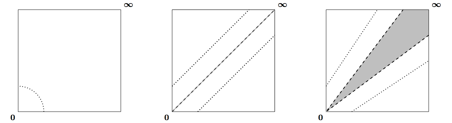
Figure 1: Left: $\mathbb{R}_{+}^{2}\setminus\{\boldsymbol{0}\}$ and distance is $L_{2}$. Center: $\mathbb{R}_{+}^{2}\setminus[{\textsf{diag}}]$ and distance is $L_{2}$. Right: $\mathbb{R}_{+}^{2}\setminus[\textsf{wedge}]$ and distance is $L_{2}$. The dotted lines represent $\aleph_{\mathbb{C}_{0}}$ which is the locus of points at distance one from $\mathbb{C}_{0}$.

1. For $\mathbb{R}_{{+}}^{2}\setminus\{\boldsymbol{0}\}$, where the forbidden zone is $\{\boldsymbol{0}\}$, we have $\aleph_{\boldsymbol{0}}=\{\boldsymbol{x}\in\mathbb{R}_{{+}}^{2}:d(\boldsymbol{x},\{\boldsymbol{0}\})=1\}$.

2. If we delete the forbidden zone $\mathbb{C}_{0}=[\textsf{diag}]=\{(x,x):x\in\mathbb{R}_{{+}}\}$ from $\mathbb{R}_{{+}}^{2}$, the appropriate unit sphere with respect to $L_{2}$ distance is

   $$\aleph_{[\textsf{diag}]}:=\aleph_{>[\textsf{diag}]}\cup\aleph_{<[\textsf{diag}]}=\{(u,u+\sqrt{2}):{u\geqslant 0}\}\bigcup\{(u,u-\sqrt{2}):{u\geqslant\sqrt{2}}\},$$ (2.9)

   the lines of slope 1, above and below the diagonal, which are at distance 1 from the diagonal. For $\boldsymbol{x}\notin[\textsf{diag}]$,

   $$d\bigl{(}\boldsymbol{x},[\textsf{diag}]\bigr{)}=|x_{1}-x_{2}|/\sqrt{2}.$$ (2.10)

3. When the forbidden zone is $[\textsf{wedge}]\subset\mathbb{R}_{+}^{2}$, we have

   $$\aleph_{[\textsf{wedge}]}= \aleph_{>[\textsf{wedge}]}\cup\aleph_{<[\textsf{wedge}]}$$

   $$= \{(u,a_{u}u+\sqrt{1+a_{u}^{2}}):u\geqslant 0\}\bigcup\{(u,a_{l}u-\sqrt{1+a_{l}^{2}}):u\geqslant a_{l}^{-1}\sqrt{1+a_{l}^{2}}\},$$ (2.11)

   which are the lines parallel to the two rays defining $[\textsf{wedge}]$ at a distance of 1 from $[\textsf{wedge}]$. When $a_{l}=a_{u}=1$, $\aleph_{[\textsf{wedge}]}$ reduces to $\aleph_{[\textsf{diag}]}$. For the distance to the forbidden zone from a point $\boldsymbol{x}\notin[\textsf{wedge}]$, we have

   $$d\bigl{(}\boldsymbol{x},[\textsf{wedge}]\bigr{)}= \frac{|x_{2}-a_{u}x_{1}|}{\sqrt{1+a_{u}^{2}}}, \text{ if }x_{2}>a_{u}x_{1},$$ (2.12)

   $$d\bigl{(}\boldsymbol{x},[\textsf{wedge}]\bigr{)}= \frac{|x_{2}-a_{l}x_{1}|}{\sqrt{1+a_{l}^{2}}}, \text{ if }x_{2}<a_{l}x_{1},$$ (2.13)

   which reduces to (2.10) if $a_{l}=a_{u}=1$.

Obvious changes apply when the state space is $\mathbb{R}^{2}$.

3 MRV and HRV under strong asymptotic dependence.

3.1 Definitions.

Consider simultaneous existence of regular variation on both the big cone $\mathbb{R}_{+}^{2}\setminus\{\boldsymbol{0}\}$ and a smaller cone $\mathbb{R}_{+}^{2}\setminus\mathbb{C}_{0}$, where $\mathbb{C}_{0}$ is either $[\textsf{diag}]$ or $[\textsf{wedge}]$. We provide equivalent polar-coordinate conditions for this simultaneous existence.

Definition 3.1.

The vector $\boldsymbol{Z}$ is regularly varying on $\mathbb{R}_{+}^{2}\setminus\{\boldsymbol{0}\}$ and has hidden regular variation on $\mathbb{R}_{+}^{2}\setminus\mathbb{C}_{0}$ if there exist $0<\alpha\leqslant\alpha_{0}$, scaling functions $b(t)\in\mathcal{RV}_{1/\alpha}$ and $b_{0}(t)\in\mathcal{RV}_{1/\alpha_{0}}$ with $b(t)/b_{0}(t)\to\infty$ and limit measures $\nu,\,\nu_{0}$ such that

$$\boldsymbol{Z}\in\text{MRV}(\alpha,b(t),\nu,\mathbb{R}_{+}^{2}\setminus\{\boldsymbol{0}\})\cap\text{MRV}(\alpha_{0},b_{0}(t),\nu_{0},\mathbb{R}_{+}^{2}\setminus\mathbb{C}_{0}).$$ (3.1)

Unpacking the notation we obtain the two regular variation limits

$$t\mathbb{P}[\boldsymbol{Z}/b(t)\in\cdot\,]\to \,\nu(\cdot) \quad\text{ in }\mathbb{M}(\mathbb{R}_{+}^{2}\setminus\{\boldsymbol{0}\}),$$ (3.2)

$$t\mathbb{P}[\boldsymbol{Z}/b_{0}(t)\in\cdot\,]\to \,\nu_{0}(\cdot) \quad\text{ in }\mathbb{M}(\mathbb{R}_{+}^{2}\setminus\mathbb{C}_{0}).$$ (3.3)

Using polar coordinates, (3.2) can be written as

$$t\mathbb{P}\left[\left(\|\boldsymbol{Z}\|/b(t),\boldsymbol{Z}/\|\boldsymbol{Z}\|\right)\in\cdot\,\right]\to \,\nu_{\alpha}\times S(\cdot) \quad\text{ in }\mathbb{M}((0,\infty)\times\aleph_{\boldsymbol{0}}),$$ (3.4)

where $S$ is a probability measure on $\aleph_{\boldsymbol{0}}$. Similarly when removing $\mathbb{C}_{0}$ from the state space, generalized polar coordinates allow re-writing (3.3) as

$$t\mathbb{P}\Bigl{[}\Bigl{(}\frac{d(\boldsymbol{Z},\mathbb{C}_{0})}{b_{0}(t)},\frac{\boldsymbol{Z}}{d(\boldsymbol{Z},\mathbb{C}_{0})}\Bigr{)}\in\cdot\,\Bigr{]}\to(\nu_{\alpha_{0}}\times S_{0})(\cdot)$$ (3.5)

in $\mathbb{M}\left((0,\infty)\times\aleph_{\mathbb{C}_{0}}\right)$ where $\nu_{\alpha_{0}}(x,\infty)=x^{-\alpha_{0}},\,x>0,\,\alpha_{0}>0$ and $S_{0}(\cdot)$ is a probability measure on $\aleph_{\mathbb{C}_{0}}$.

3.2 Regular variation when deleting $[\textsf{wedge}]$.

Focus on the special case where the forbidden zone is $[\textsf{wedge}]$. Since $[\textsf{diag}]$ is a particular case of $[\textsf{wedge}]$, we do not treat $[\textsf{diag}]$ separately. Recall the notation in (2.11) and the two parameterizations of $[\textsf{wedge}]$ given in (2.1), (2.2) and (2.3). The distance of points to $[\textsf{wedge}]$ is given in (2.12) and (2.13). When $\mathbb{C}_{0}=[\textsf{wedge}]$, (3.5) becomes two statements. With $x>0$ and $\Lambda\subset\aleph_{[\textsf{wedge}]}$ we have

$$t\mathbb{P}\left[\frac{Z_{2}-a_{u}Z_{1}}{{b_{0}(t)}\sqrt{1+a_{u}^{2}}}>x,\frac{\sqrt{1+a_{u}^{2}}\boldsymbol{Z}}{Z_{2}-a_{u}Z_{1}}\in\Lambda\right]\to x^{-\alpha_{0}}S_{0}(\Lambda) \quad\text{ in }\mathbb{M}\left((0,\infty)\times\aleph_{>[\textsf{wedge}]}\right),$$ (3.6)

$$t\mathbb{P}\left[\frac{a_{l}Z_{1}-Z_{2}}{{b_{0}(t)}\sqrt{1+a_{l}^{2}}}>x,\frac{\sqrt{1+a_{l}^{2}}\boldsymbol{Z}}{a_{l}Z_{1}-Z_{2}}\in\Lambda\right]\to x^{-\alpha_{0}}S_{0}(\Lambda) \quad\text{ in }\mathbb{M}\left((0,\infty)\times\aleph_{<[\textsf{wedge}]}\right).$$ (3.7)

Modifying variables leads to the two simpler statements. For $x>0$,

$$t\mathbb{P}\left[\frac{Z_{2}-a_{u}Z_{1}}{b_{0}(t)}>x,\frac{Z_{2}}{Z_{1}}\leqslant y\right]\to (1+a_{u}^{2})^{\frac{\alpha_{0}}{2}}x^{-\alpha_{0}}S_{0}\Biggl{\{}\Bigl{(}v,a_{u}v+\sqrt{1+a_{u}^{2}}\Bigr{)}:v\geqslant\frac{\sqrt{1+a_{u}^{2}}}{y-a_{u}}\Biggr{\}},\;y>a_{u},$$ (3.8)

$$t\mathbb{P}\left[\frac{a_{l}Z_{1}-Z_{2}}{b_{0}(t)}>x,\frac{Z_{1}}{Z_{2}}\leqslant y\right]\to (1+a_{l}^{2})^{\frac{\alpha_{0}}{2}}x^{-\alpha_{0}}S_{0}\Bigl{\{}\bigl{(}v+\sqrt{1+a_{l}^{2}}/a_{l},v\bigr{)}:v\geqslant\frac{\sqrt{1+a_{l}^{2}}}{a_{l}y-1}\Bigr{\}},\;y>\frac{1}{a_{l}}.$$ (3.9)

Remark 3.1.

Thus a necessary condition for non-trivial regular variation on $\mathbb{R}_{+}^{2}\setminus[\textsf{wedge}]$ is that both $(Z_{2}-a_{u}Z_{1})_{+}$ and $(a_{l}Z_{1}-Z_{2})_{+}$ be regularly varying with index $\alpha_{0}\geqslant\alpha$. This fact suggests the exploratory diagnostic of testing whether these 1 dimensional variables have power laws with the same index. If so, one can continue to explore with the Hillish statistic and associated plot; see Section 3.6.

However, there is nothing to prevent the possibility that regular variation exists on the region above $[\textsf{wedge}]$ but that tails are of lower order below $[\textsf{wedge}]$. This would happen for instance if $S_{0}(\aleph_{<[\textsf{wedge}]})=0$ but $S_{0}(\aleph_{>[\textsf{wedge}]})>0$. If this happened, one could search for another higher index or thinner tailed regular variation on $<[\textsf{wedge}].$

Remark 3.2.

Analogous statements to the limits (3.8), (3.9) hold true when $\mathbb{C}=\mathbb{R}^{2}$ and $[\textsf{diag}]$ and $[\textsf{wedge}]$ are their appropriate equivalents in $\mathbb{R}^{2}$ to get.

3.2.1 Restrictions on the choice of $[\textsf{wedge}]$.

In this paper, we assume that $1<a_{l}\leqslant 1\leqslant a_{u}<\infty$ where $[\textsf{wedge}]=\{\boldsymbol{x}\in\mathbb{R}_{+}^{2}:a_{l}x_{1}\leqslant x_{2}\leqslant a_{l}x_{1}\}$. This choice is partly governed by the fact that it is easier for us to deal with data portraying tail equivalence with $\lim_{t\to\infty}{\mathbb{P}(Z_{1}>t)}/{\mathbb{P}(Z_{2}>t)}=1.$ Now, when $a_{l}=a_{u}$, we get $[\textsf{wedge}]=[\textsf{diag}]$, which means under a model of full asymptotic dependence the only limit measure that we allow is restricted to $[\textsf{diag}]$. If we assume $\boldsymbol{Z}\in\text{MRV}(\alpha,b(t),\nu,\mathbb{R}_{+}^{2}\setminus\{\boldsymbol{0}\})$ and $\nu$ is supported on $[\textsf{diag}]$ then using (3.2), this clearly implies, that

$$\lim_{t\to\infty}\frac{\mathbb{P}(Z_{1}>t)}{\mathbb{P}(Z_{2}>t)} =\lim_{t\to\infty}\frac{\mathbb{P}(Z_{1}>b(t))}{\mathbb{P}(Z_{2}>b(t))}$$

$$=\lim_{t\to\infty}\frac{t\,\mathbb{P}\left(\boldsymbol{Z}/b(t)\in(1,\infty)\times[0,\infty)\right)}{t\,\mathbb{P}\left(\boldsymbol{Z}/b(t)\in[0,\infty)\times(1,\infty)\right)}$$

$$=\frac{\nu\left((1,\infty)\times[0,\infty)\right)}{\nu\left([0,\infty)\times(1,\infty)\right)}$$

$$=\frac{\nu\left((x_{1},x_{2}):x_{1}>1,(x_{1},x_{2})\in[\textsf{diag}]\right)}{\nu\left((x_{1},x_{2}):x_{2}>1,(x_{1},x_{2})\in[\textsf{diag}]\right)}=1,$$

where the last line is a consequence of $\nu$ being concentrated on $[\textsf{diag}]$. Thus, not only are $Z_{1},Z_{2}$ tail equivalent, but in fact $\lim_{t\to\infty}{\mathbb{P}(Z_{1}>t)}/{\mathbb{P}(Z_{2}>t)}=1.$

The following lemma shows that that we cannot choose a $[\textsf{wedge}]$ which does not contain $[\textsf{diag}]$ if we want to guarantee $\lim_{t\to\infty}{\mathbb{P}(Z_{1}>t)}/{\mathbb{P}(Z_{2}>t)}=1.$

Lemma 3.1.

If $\boldsymbol{Z}\in\text{MRV}(\alpha,b(t),\nu,\mathbb{R}_{+}^{2}\setminus\{\boldsymbol{0}\})$ where $\nu$ is supported on $[\textsf{wedge}]=\{\boldsymbol{x}\in\mathbb{R}_{+}^{2}:a_{l}x_{1}\leqslant x_{2}\leqslant a_{l}x_{1}\}$ and $\lim_{t\to\infty}{\mathbb{P}(Z_{1}>t)}/{\mathbb{P}(Z_{2}>t)}=1$ then $0<a_{l}\leqslant 1\leqslant a_{u}<\infty$.

Proof.

To get a contradiction, suppose we have $1<a_{l}\leqslant a_{u}<\infty.$ (A similar contradiction is obtained if we assume $0<a_{l}\leqslant a_{u}<1.$) Assume,

$$1=\ \lim_{t\to\infty}\frac{\mathbb{P}(Z_{1}>t)}{\mathbb{P}(Z_{2}>t)} =\lim_{t\to\infty}\frac{t\,\mathbb{P}\left(\boldsymbol{Z}/b(t)\in(1,\infty)\times[0,\infty)\right)}{t\,\mathbb{P}\left(\boldsymbol{Z}/b(t)\in[0,\infty)\times(1,\infty)\right)}=\frac{\nu\left((1,\infty)\times[0,\infty)\right)}{\nu\left([0,\infty)\times(1,\infty)\right)}.$$

Hence $\nu\left((1,\infty)\times[0,\infty)\right)=\nu\left([0,\infty)\times(1,\infty)\right)$. We know that $\nu$ is supported on $[\textsf{wedge}]$. So,

$$\nu\left((1,\infty)\times[0,\infty)\right) =\nu((x_{1},x_{2})\in\mathbb{R}_{+}^{2}:x_{1}>1,(x_{1},x_{2})\in[\textsf{wedge}])$$

$$=\nu\left((x_{1},x_{2})\in\mathbb{R}_{+}^{2}:x_{1}>1,a_{l}\leqslant\frac{x_{2}}{x_{1}}\leqslant a_{u}\right)$$

$$<\nu\left((x_{1},x_{2})\in\mathbb{R}_{+}^{2}:x_{1}>{\frac{1}{a_{l}}},a_{l}\leqslant\frac{x_{2}}{x_{1}}\leqslant a_{u}\right) (\text{since $a_{l}>1$})$$

$$<\nu\left((x_{1},x_{2})\in\mathbb{R}_{+}^{2}:x_{2}>1,a_{l}\leqslant\frac{x_{2}}{x_{1}}\leqslant a_{u}\right) x_{2}\geqslant a_{l}x_{1}$$ (since )

$$=\nu\left([0,\infty)\times(1,\infty)\right),$$

which is a contradiction. ∎

3.3 Regular variation when deleting $[\textsf{wedge}]$ expressed in traditional polar coordinates.

Regular variation on $\mathbb{R}_{+}^{2}\setminus[\textsf{wedge}]$ expressed using generalized polar coordinates in (3.8), (3.9) can also be written in terms of the traditional polar coordinates $\boldsymbol{z}\mapsto\bigl{(}r,(\theta,1-\theta)\bigr{)}$ where $z_{1}=r\theta$ and $z_{2}=r(1-\theta)$ and $r=z_{1}+z_{2}.$ Using capital letters for random variables, the left most probability in (3.8) becomes for $x>0,\,y>a_{u}$,

$$t\mathbb{P}\Bigl{[}\frac{Z_{2}-a_{u}Z_{1}}{b_{0}(t)}>x, \frac{Z_{2}}{Z_{1}}\leqslant y\Bigr{]}=t\mathbb{P}\left[\frac{R(1-\Theta(1+a_{u}))}{b_{0}(t)}>x,\frac{(1-\Theta)}{\Theta}\leqslant y\right]$$

and using (2.1) this is

$$= t\mathbb{P}\left[\frac{R(1-\theta_{l}^{-1}\Theta)}{b_{0}(t)}>x,\Theta^{-1}\leqslant y+1\right]=t\mathbb{P}\left[\frac{R(1-\theta_{l}^{-1}\Theta)}{b_{0}(t)}>x,\Theta\geqslant\frac{1}{1+y}\right]$$

Set $s=1/(1+y)$ where $y>a_{u}$ and thus $s<\theta_{l}$,

$$t\mathbb{P}\left[\frac{R(1-\theta_{l}^{-1}\Theta)}{b_{0}(t)}>x,\Theta>s\right]\to(1+a_{u}^{2})^{\frac{\alpha_{0}}{2}}x^{-\alpha_{0}}S_{0}\Biggl{\{}\Bigl{(}v,a_{u}v+\sqrt{1+a_{u}^{2}}\Bigr{)}:v\geqslant\frac{\sqrt{1+a_{u}^{2}}}{s^{-1}-\theta_{l}^{-1}}\Biggr{\}}.$$

An analogous expression holds for (3.9). So if regular variation with index $\alpha$ holds on $\mathbb{R}_{+}^{2}\setminus\{\boldsymbol{0}\}$, $R$ is a random variable with regularly varying distribution tail with index $\alpha$ and multiplying $R$ by $1-\theta_{l}^{-1}\Theta$ produces a variable with a lighter tail having index $\alpha_{0}$.

3.4 The forbidden zone of HRV and the limit measure on $\mathbb{E}$.

Suppose there are two regular variation properties that hold for a vector $\boldsymbol{Z}\geqslant 0$ so that (3.1) holds with $b(t)/b_{0}(t)\to\infty$. If $\mathbb{C}_{0}=[\textsf{wedge}]$ with $0<a_{l}\leqslant 1\leqslant a_{u}<\infty$; then $\nu$, the limit measure on $\mathbb{R}_{+}^{2}\setminus\{\boldsymbol{0}\}$, must concentrate on the forbidden zone $[\textsf{wedge}]$ used to define the second regular variation. (Cf. [25, p. 324-5].) This means that when detecting MRV, if the limit measure is typical of strong asymptotic dependence and concentrates on $[\textsf{wedge}]$, we are encouraged to look for additional regular variation regimes on $\mathbb{R}_{+}^{2}\setminus[\textsf{wedge}]$. Hence we get the following result.

Proposition 3.1.

Suppose

$$\boldsymbol{Z}\in\text{MRV}(\alpha,b(t),\nu,\mathbb{R}_{+}^{2}\setminus\{\boldsymbol{0}\})\cap\text{MRV}(\alpha_{0},b_{0}(t),\nu_{0},\mathbb{R}_{+}^{2}\setminus[\textsf{wedge}])$$ (3.10)

with $b(t)/b_{0}(t)\to\infty$ and $0{<}a_{l}\leqslant 1\leqslant a_{u}<\infty.$ Then $\nu$, the limit measure on $\mathbb{R}_{+}^{2}\setminus\{\boldsymbol{0}\}$, concentrates on $[\textsf{wedge}]$.

Proof.

To see this, consider the region above the ray $y=a_{u}x$. Then for $\delta>0$, as $t\to\infty$, referring to (3.8),

$$t\mathbb{P}\Bigl{[}\frac{Z_{2}-a_{u}Z_{1}}{b(t)}>\delta\Bigr{]}= t\mathbb{P}\Bigl{[}\frac{Z_{2}-a_{u}Z_{1}}{b_{0}(t)}>\frac{b(t)}{b_{0}(t)}\delta\Bigr{]}\to 0,$$

since $b(t)/b_{0}(t)\to\infty$ and $S_{0}(\cdot)$ is a probability measure. Similarly, for the region below the ray $y=a_{l}x$,

$$t\mathbb{P}\Bigl{[}\frac{a_{l}Z_{1}-Z_{2}}{b(t)}>\delta\Bigr{]}= t\mathbb{P}\Bigl{[}\frac{a_{l}Z_{1}-Z_{2}}{b_{0}(t)}>\frac{b(t)}{b_{0}(t)}\delta\Bigr{]}\to 0,$$

from (3.9). Thus $\nu$ places no mass outside $[\textsf{wedge}]$. ∎

Clearly, a result analogous to Proposition 3.1 holds where $\mathbb{C}=\mathbb{R}^{2}$ and $\mathbb{C}_{0}$ is the appropriate equivalent of $[\textsf{diag}]$ and $[\textsf{wedge}]$ on $\mathbb{R}^{2}$.

3.5 How HRV on $\mathbb{R}^{2}\setminus[\textsf{wedge}]$ can improve risk estimates.

Suppose $I_{1}$ and $I_{2}$ are financial instruments that have positive risks $Z_{1}$ and $Z_{2}$ per unit of investment where $\boldsymbol{Z}=(Z_{1},Z_{2})$ satisfies (3.10). Suppose we buy one unit of $I_{2}$ and sell $2a_{l}$ units of $I_{1}$. The risk of this portfolio is $Z_{2}-2a_{l}Z_{1}$ and we have two asymptotic regimes that can be used to estimate the probability the risk is large. If we use MRV with scale function $b(t)$ then for large $x>0$,

$$\mathbb{P}[Z_{2}-2a_{u}Z_{1}>x]= \mathbb{P}\Bigl{[}\Bigl{(}\frac{Z_{1}}{b(t)},\frac{Z_{2}}{b(t)}\Bigr{)}\in\{(v,w)\in\mathbb{R}_{+}^{2}:w-2a_{u}v>x/b(t)\}\Bigr{]}$$

$$\approx \frac{1}{t}\nu\{(v,w)\in\mathbb{R}_{+}^{2}:w-2a_{u}v>x/b(t)\}=0$$

since the required region is outside the support $$[\textsf{wedge}] \nu 0 b_{0}(t)$$ of the measure . Is the risk really or did we use the wrong asymptotic approximation? If we use HRV with scale function , then we get a non-zero limit:

$$\mathbb{P}[Z_{2}-2a_{u}Z_{1}>x]= \mathbb{P}\Bigl{[}\Bigl{(}\frac{Z_{1}}{b_{0}(t)},\frac{Z_{2}}{b_{0}(t)}\Bigr{)}\in\{(v,w)\in\mathbb{R}_{+}^{2}:w-2a_{u}v>x/b_{0}(t)\}\Bigr{]}$$

$$\approx \frac{1}{t}\nu_{0}\{(v,w)\in\mathbb{R}_{+}^{2}:w-2a_{u}v>x/b_{0}(t)\}.$$

Now switch to generalized polar coordinates with $$(v,w)=r(\mu_{1},\mu_{2}) \mu_{2}=a_{u}\mu_{1} \nu_{\alpha_{0}}\times S_{0}\bigl{(}d(\mu_{1},\mu_{2})\bigr{)}$$ and and the risk calculation is with respect to the product measure and

$$\mathbb{P}[Z_{2}-2a_{u}Z_{1}>x]\approx \frac{1}{t}\iint_{\{(r,(\mu_{1},\mu_{2})):r\mu_{2}-2a_{u}r\mu_{1}>x/b_{0}(t)\}}\alpha_{0}r^{-\alpha_{0}-1}S_{0}\bigl{(}\mathrm{d}(\mu_{1},\mu_{2})\bigr{)}$$

$$= \frac{1}{t}\Bigl{(}\frac{x}{b_{0}(t)}\Bigr{)}^{-{\alpha_{0}}}\int_{\{(\mu_{1},\mu_{2}):\mu_{2}-2a_{u}\mu_{1}>0\}}(\mu_{2}-2a_{u}\mu_{1})^{\alpha_{0}}S_{0}\bigl{(}\mathrm{d}(\mu_{1},\mu_{2})\bigr{)}.$$

Of course, in practice $S_{0},\alpha_{0},b_{0}$ must be replaced by estimators and $t$ is replaced by $n/k$ where $n$ is the sample size of observations and $k$ is the number of observations used in estimation. An example where we carry out these calculations is given for simulated data in Section 4.2.1.

3.6 Exploring for HRV with the Hillish estimator.

The Hillish estimator was designed for detection of the CEV model [16; 18; 17; 23; 8; 10; 9] and extended to detecting hidden regular variation in [11]. The generalized polar coordinate transform converts Cartesian coordinates in the definition of regular variation into coordinates satifying the CEV model. In this paper we show that the Hillish technique can detect HRV when the cone removed from $\mathbb{R}^{2}_{+}$ or $\mathbb{R}^{2}$ is $[\textsf{wedge}]$. The Hillish procedure is described below. First we define a conditional extreme value model.

3.6.1 The CEV model.

Suppose the random variables $(\xi,\eta)$ form a random element of $\mathbb{R}_{+}\times\mathbb{R}$ and there exists a regularly varying function $b(t)\to\infty$ and a non-null measure $\mu\in\mathbb{M}((0,\infty)\times\mathbb{R})$ and

$$t\mathbb{P}\Bigl{[}\Bigl{(}\frac{\xi}{{b}(t)},{\eta}\Bigr{)}\in\;\cdot\;\Bigr{]}\to\mu(\cdot),\qquad\text{ in }\mathbb{M}((0,\infty)\times\mathbb{R}).$$ (3.11)

Note that (2.8) is of this form where only the first component $\xi=d(\boldsymbol{Z},\mathbb{C}_{0})$ is scaled. See also (3.8) and (3.9). Additionally assume that

• $\mu((r,\infty]\times\cdot\,)$ is a non-degenerate measure for any fixed $r>0$, and,

• $H(\cdot):=\mu((1,\infty)\times\cdot\,)$ is a probability distribution.

Then $(\xi,\eta)$ satisfies a conditional extreme value model and we write $(\xi,\eta)\in\text{CEV}({b},\mu)$. Note (3.8) and (3.9) are of the form given in (3.11). Hence the HRV statements are equivalent to the appropriate transforms of the variables following a CEV model.

3.6.2 The Hillish procedure.

Now suppose $(\xi_{i},\eta_{i});1\leqslant i\leqslant n$ are iid replicates of $(\xi,\eta)$. Define

$$\begin{array}[]{llll}\xi_{(1)}\geqslant\ldots\geqslant\xi_{(n)}&\text{The decreasing order statistics of $\xi_{1},\ldots,\xi_{n}$.}\\[2.84526pt] \eta_{i}^{*},~{}1\leqslant i\leqslant n&\text{The $\eta$-variable corresponding to $\xi_{(i)}$, also called}\\[2.84526pt] &\text{ the concomitant of $\xi_{(i)}$.}\\[2.84526pt] N_{i}^{k}=\sum\limits_{l=i}^{k}\boldsymbol{1}_{\{\eta_{l}^{*}\leqslant\eta_{i}^{*}\}}&\text{Rank of $\eta^{*}_{i}$ among $\eta_{1}^{*},\ldots,\eta_{k}^{*}$. We write $N_{i}=N_{i}^{k}$.}\\[2.84526pt] \eta_{1:k}^{*}\leqslant\eta_{2:k}^{*}\leqslant\ldots\leqslant\eta_{k:k}^{*}&\text{The increasing order statistics of $\eta_{1}^{*},\ldots,\eta_{k}^{*}$.}\\[2.84526pt] \end{array}$$

By analogy with the Hill estimator and the Hill plot, the Hillish statistic is defined for $1\leqslant k\leqslant n$ as

$$\text{Hillish}_{k,n}=\text{Hillish}_{k,n}(\mathbb{\xi},\mathbb{\eta}):=\frac{1}{k}\sum\limits_{j=1}^{k}\log\frac{k}{j}\log\frac{k}{N_{j}^{k}}$$ (3.12)

According to [10, Propositions 2.2 and 2.3], if $(\xi,\eta)\in\text{CEV}(b,\mu)$ then there exists a limit $I_{\mu}$ and $\text{Hillish}_{k,n}\stackrel{{\scriptstyle P}}{{\to}}I_{\mu}$ and moreover, $\mu$ is a product measure iff both

$$\text{Hillish}_{k,n}(\mathbb{\xi},\mathbb{\eta})\stackrel{{\scriptstyle\lower 0.60275pt\hbox{$\scriptscriptstyle\it{P}$}}}{{\rightarrow}}1\quad\text{and}\quad\text{Hillish}_{k,n}(\mathbb{\xi},-\mathbb{\eta})\stackrel{{\scriptstyle\lower 0.60275pt\hbox{$\scriptscriptstyle\it{P}$}}}{{\rightarrow}}1,$$ (3.13)

as $k\to\infty,n\to\infty,n/k\to\infty$. Note the limits in (3.8), (3.9) are all product measures. Hence the diagnostic for detecting regular variation with a specified forbidden zone for the random vector $\boldsymbol{Z}$ is to plot the Hillish statistic of $\text{GPOLAR}(\boldsymbol{Z})$.

We emphasize that if (3.13) holds, we have empirical behavior consistent with the presence of regular variation but this does not prove existence of regular variation. When the Hillish technique fails because the plots do not hug the line at height 1, we can reject a hypothesis of regular variation.

4 Data Analysis with Simulated Data

Before moving to real data, we test our analysis techniques on two simulated data sets to see how well they perform in Section 4.1 and 4.2. Further, we discuss MRV and HRV properties and their detection. In Section 5, we analyze two real bivariate data sets both of which exhibit heavy-tailed margins and strong asymptotic dependence.

4.1 Example 1: Full asymptotic dependence.

Suppose $Z_{1}\sim$ Pareto(1.5) and $Z_{2}\sim$ Pareto(2.5) and independent of each other. Let $B_{1},B_{2}$ be iid Bernoulli (0.5) random variables also independent of $Z_{1}$ and $Z_{2}$. Now define the vector $\boldsymbol{X}=(X_{1},X_{2})$ as

$$X_{1} =B_{1}Z_{1}+(1-B_{1})Z_{2},$$

$$X_{2} =B_{1}Z_{1}+B_{2}(1-B_{1})(1.5Z_{2})+(1-B_{2})(1-B_{1})(0.5Z_{2})$$

Figure 2: Example 4.1: (Left) Scatter plot of 10,000 data points. (Center and right) Hill plots for tail parameters of the marginal distributions of $X_{1}$ (center) and $X_{2}$ (right).The horizonal lines are at height $1.5.$

By construction

$${\boldsymbol{X}=\begin{cases}(Z_{1},Z_{1}),&\text{ with probability }P[B_{1}=1]=\frac{1}{2},\\ (Z_{2},1.5Z_{2}),&\text{ with probability }P[B_{1}=0,B_{2}=1]=\frac{1}{4},\\ (Z_{2},0.5Z_{2}),&\text{ with probability }P[B_{1}=0,B_{2}=0]=\frac{1}{4},\\ \end{cases}}$$

so that $\boldsymbol{X}=(X_{1},X_{2})$ lies on $y=x$ with probability 0.5. With probability 0.25 each it is either on the line $y=0.5x$ or on $y={1.5}x$. In this model, $\boldsymbol{X}$ is MRV with parameter $\alpha=1.5$ and it has full dependence on the diagonal $[\textsf{diag}]:=\{(x,y)\in\mathbb{R}_{+}^{2}:y=x\}$. On the other hand, on $\mathbb{R}^{2}_{+}\setminus[\textsf{diag}]$,

$$t\,\mathbb{P}\left(\frac{d((X_{1},X_{2}),[\textsf{diag}])}{t^{1/2.5}/2\sqrt{2}}>x,\frac{(X_{1},X_{2})}{\sqrt{2}d((X_{1},X_{2}),[\textsf{diag}])}=\boldsymbol{a}\right) =t\,\mathbb{P}\left(\frac{(2|X_{1}-X_{2}|}{t^{1/2.5}}>x,\frac{(X_{1},X_{2})}{|X_{1}-X_{2}|}=\boldsymbol{a}\right)$$

$$\to x^{{-2.5}}\times\frac{1}{4}=\frac{1}{2}\nu_{{2.5}}(x,\infty)S_{{0}}(\{{\sqrt{2}\boldsymbol{a}}\}).$$

where $\boldsymbol{a}=(2,1)$ or $(2,3)$ and $S_{0}(\sqrt{2}\boldsymbol{a})=0.5$. Hence we have HRV on $\mathbb{R}_{+}^{2}\setminus[\textsf{diag}]$ with tail parameter $\alpha_{0}=2.5$.

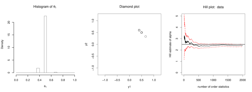
Figure 3: Example 4.1: Histogram of $\theta_{1}$ (left), diamond plot (center), and Hill plot for tail estimate of $|X_{1}-X_{2}|$ (right). The horizontal line is at height 2.5.

We generate $n=10,000$ iid samples from this data set. The scatter plot in Figure 2 shows the dependence structure of $\boldsymbol{X}$ along with Hill plots of $X_{1},X_{2}$ which supports the premise that $\alpha=1.5$.

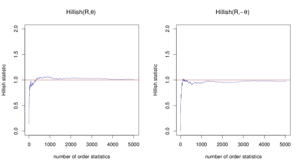
Figure 4: Example 4.1: Hillish plots for $(\xi,\eta)$ (left) and $(\xi,-\eta)$ (right) where $(\xi,\eta)=(|X_{1}-X_{2}|,X_{1}/|X_{1}-X_{2}|)$.

To understand the dependence structure of the variables $\boldsymbol{X}$, we make the diamond plot, the transformation from $\mathbb{R}^{2}\mapsto\aleph_{\boldsymbol{0}}\subset\mathbb{R}^{2}$ onto the $L_{1}$ unit sphere represented by the diamond $\{(\theta_{1},\theta_{2}):|\theta_{1}|+|\theta_{u}|=1\}$ We do the mapping at various thresholds determined by $k$, the number of order statistics of the norms $\|\boldsymbol{x}\|=|x_{1}|+|x_{2}|$. In Figure 3, the diamond plot and histogram of the angular measure is shown for $k=100$. Clearly the data is concentrated at $x=y$. The Hill plot of the quantity $|X_{1}-X_{2}|$ supports the fact that data was generated with hidden tail parameter $\alpha_{0}=2.5$.

Finally, we look at the Hillish statistic for $(\xi,\eta)=(|X_{1}-X_{2}|,X_{1}/|X_{1}-X_{2}|)$ after removing $[\textsf{diag}]$. The Hillish plot in Figure 4 is convincingly stable and close to 1, supporting the presence of HRV as expected from the generation procedure here.

4.2 Example 2: Strong asymptotic dependence.

In this example, we simulate data from a model with strong asymptotic dependence. We also exhibit estimation of rare probabilities and conduct a sensitivity analysis when the support of the regular variation for the the first level, and hence that for HRV is not correctly identified.

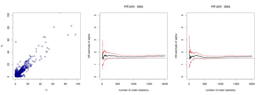
Figure 5: Example 4.2: (Left) Scatter plot of 30,000 data points. (Center and right) Hill plots for tail parameters of the marginal distributions of $X_{1},X_{2}$. The horizontal lines are at height $1.5$.

Suppose $R_{1}\sim$ Pareto(1.5) and $R_{2}\sim$ Pareto(2.5) and independent of each other. Let $\Theta_{1}\sim\text{Unif}[0.4,0.6]$, $\Theta_{2}\sim\text{Unif}([0,1]\setminus[0.4,0.6)]$, $B\sim$ Bernoulli (0.5) random variables. Assume the random variables are all independent. Now define the vector $\boldsymbol{X}=(X_{1},X_{2})$ as

$$X_{1} =BR_{1}\Theta_{1}+(1-B)R_{2}\Theta_{2},$$

$$X_{2} =BR_{1}(1-\Theta_{1})+(1-B)R_{2}(1-\Theta_{2}).$$

By construction, $\boldsymbol{X}$ is MRV on $\mathbb{R}_{+}^{2}\setminus\{\boldsymbol{0}\}$ with tail parameter $\alpha=1.5$. Corresponding to $(\theta_{l},\theta_{u})=(0.4,0.6)$, we have by (2.1) that $(a_{l},a_{u})=(0.67,1.5)$ and therefore

$$[\textsf{wedge}]:=\{(x,y)\in\mathbb{R}_{+}^{2}:0.67x\leqslant y\leqslant 1.5x\}.$$

This gives hidden regular variation with tail parameter $\alpha_{0}=2.5$ on $\mathbb{R}_{+}^{2}\setminus[\textsf{wedge}]$.

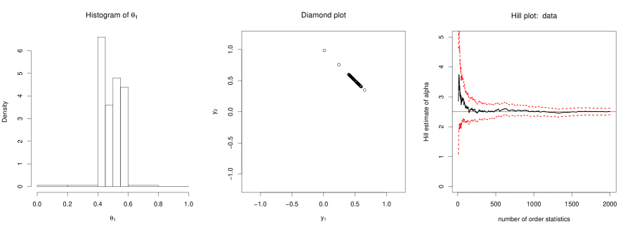
Figure 6: Example 4.2: Diamond plot, histogram and Hill plot for tail estimate of $d(\boldsymbol{X},[\textsf{wedge}])$. The horizontal line in the Hill plot is at height 2.5.

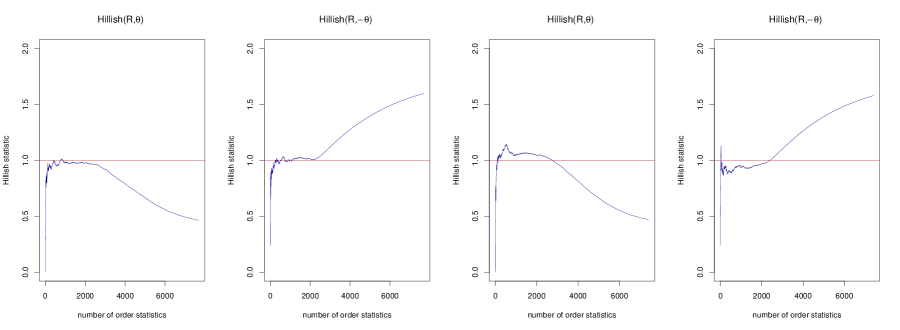
Figure 7: Example 4.2: Hillish plots for (i)$(\xi_{1},\eta_{1}),$ (ii)$(\xi_{1},-\eta_{1})$, (iii)$(\xi_{2},\eta_{2}),$ (iv)$(\xi_{2},-\eta_{2})$ respectively where $(\xi_{1},\eta_{1})$ and $(\xi_{2},\eta_{2})$ are obtained by using (3.8) and (3.9) on $\boldsymbol{X}=(X_{1},X_{2})$.

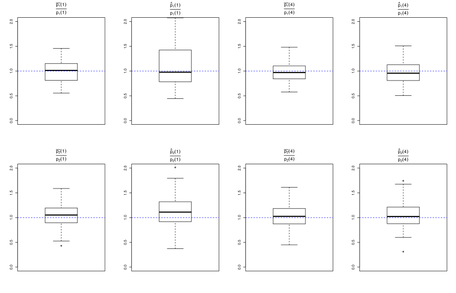
Figure 8: Example 4.2: Boxplots for $\frac{\bar{p}_{1}(1)}{p_{1}(1)},\frac{\hat{p}_{1}(1)}{p_{1}(1)},\frac{\bar{p}_{1}(4)}{p_{1}(1)},\frac{\hat{p}_{1}(4)}{p_{1}(4)}$ (top) and $\frac{\bar{p}_{2}(1)}{p_{2}(1)},\frac{\hat{p}_{2}(1)}{p_{2}(1)},\frac{\bar{p}_{2}(4)}{p_{2}(4)},\frac{\hat{p}_{2}(4)}{p_{2}(4)}$ (bottom) .

We generate $n=30,000$ iid samples from this data set. The scatter plot in Figure 5 shows the dependence structure of $\boldsymbol{X}$ along with Hill plots of $X_{1},X_{2}$ which supports the premise that $\alpha=1.5$.

To understand the dependence structure of $\boldsymbol{X}$, we graph the diamond plot as used in the previous example. We do the mapping at various thresholds determined by $k$, the number of order statistics of the norms $|x|+|y|$. In Figure 6, the histogram of angles and the diamond plot are shown for $k=100$ and shows the angles are Uniform in [0.4, 0.6] for high values of $|x|+|y|$. The Hill plot of the quantity $d(\boldsymbol{X},[\textsf{wedge}])$ supports the fact that data was generated with hidden tail parameter $\alpha_{0}=2.5$. Finally, we look at a Hillish statistic for $(\xi_{1},\eta_{1})$ and $(\xi_{2},\eta_{2})$ respectively which are obtained by using (3.8) and (3.9) on $\boldsymbol{X}=(X_{1},X_{2})$ after removing $[\textsf{wedge}]$. The Hillish plots in Figure 7 are again convincingly stable and close to 1 and detect the hidden regular variation.

4.2.1 Probabilities of rare sets for this example.

Now to further illustrate our methods, we compute $\mathbb{P}(X_{2}-2X_{1}>x)$ and $\mathbb{P}(X_{2}-3X_{1}>x)$. Without resorting to hidden regular variation we have $\boldsymbol{X}$ is MRV on $\mathbb{R}_{+}^{2}\setminus\{\boldsymbol{0}\}$ with tail parameter $\alpha=1.5$ and the limit measure concentrates on

$$[\textsf{wedge}]:=\{\boldsymbol{x}\in\mathbb{R}_{+}^{2}:a_{l}x_{1}\leqslant x_{2}\leqslant a_{u}x_{1}\}=\{\boldsymbol{x}\in\mathbb{R}_{+}^{2}:0.67x_{1}\leqslant x_{2}\leqslant 1.5x_{1}\}.$$

Hence with the usual regular variation techniques we would estimate both

$$\mathbb{P}(X_{2}-2X_{1}>x)\approx 0\quad\text{and}\quad\mathbb{P}(X_{2}-3X_{1}>x)\approx 0.$$

But for this example we can compute the exact answer without resorting to asymptotic approximations and we get,

$$p_{1}(x):= \mathbb{P}(X_{2}-2X_{1}>x)=\frac{1}{2}\mathbb{P}(R_{1}(1-\Theta_{1}){-}2R_{1}\Theta_{1}>x)+\frac{1}{2}\mathbb{P}(R_{2}(1-\Theta_{2}){-}2R_{2}\Theta_{2}>x)$$

and because $$3\Theta_{1}>1$$, this is

$$= \frac{1}{2}\mathbb{P}(R_{2}(1-3\Theta_{2})>x)=\frac{5}{84}x^{{-2.5}}.$$ (4.1)

Similarly we can compute

$$p_{2}(x):= \mathbb{P}(X_{2}-{3}X_{1}>x)=\frac{5}{112}x^{{-2.5}}.$$ (4.2)

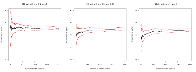
Figure 9: Example 4.2: Hill plots for estimating $\alpha_{0}$ (known to be 2.5 in the model) when the support set of MRV is incorrectly specified as $(a_{l},a_{u})=(0.5,2)$ (left), $(a_{l},a_{u})=(0.9,1.11)$ (middle), $(a_{l},a_{u})=(1,1)$ (right) respectively. The horizontal line in the Hill plot is at height 2.5.

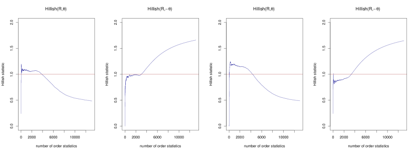
Figure 10: Example 4.2: Hillish plots for (i)$(\xi_{1},\eta_{1}),$ (ii)$(\xi_{1},-\eta_{1})$, (iii)$(\xi_{2},\eta_{2}),$ (iv)$(\xi_{2},-\eta_{2})$ respectively where $(\xi_{1},\eta_{1})$ and $(\xi_{2},\eta_{2})$ are obtained by using (3.8) and (3.9) on $\boldsymbol{X}=(X_{1},X_{2})$ and the support of MRV is (incorrectly) identified by $(a_{l},a_{u})=(0.9,1.11)$.

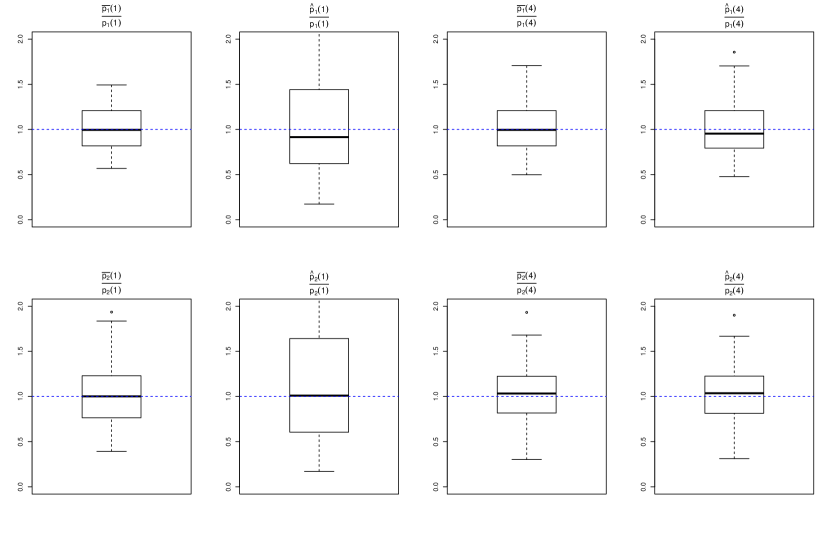
Figure 11: Example 4.2: Boxplots for $\frac{\bar{p}_{1}(1)}{p_{1}(1)},\frac{\hat{p}_{1}(1)}{p_{1}(1)},\frac{\bar{p}_{1}(4)}{p_{1}(4)},\frac{\hat{p}_{1}(4)}{p_{1}(4)}$ (top) and $\frac{\bar{p}_{2}(1)}{p_{2}(1)},\frac{\hat{p}_{2}(1)}{p_{2}(1)},\frac{\bar{p}_{2}(4)}{p_{2}(4)},\frac{\hat{p}_{2}(4)}{p_{2}(4)}$ (bottom) with (incorrect) identification of support where $a_{l}=0.5,a_{u}=2$.

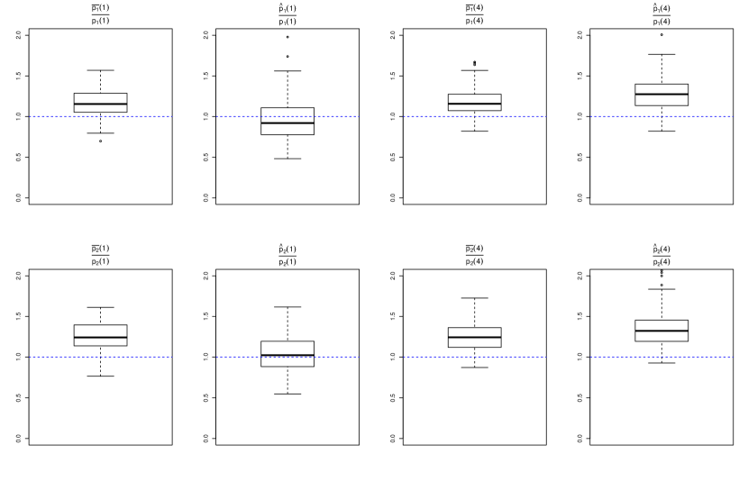
Figure 12: Example 4.2: Boxplots for $\frac{\bar{p}_{1}(1)}{p_{1}(1)},\frac{\hat{p}_{1}(1)}{p_{1}(1)},\frac{\bar{p}_{1}(4)}{p_{1}(1)},\frac{\hat{p}_{1}(4)}{p_{1}(4)}$ (top) and $\frac{\bar{p}_{2}(1)}{p_{2}(1)},\frac{\hat{p}_{2}(1)}{p_{2}(1)},\frac{\bar{p}_{2}(4)}{p_{2}(4)},\frac{\hat{p}_{2}(4)}{p_{2}(4)}$ (bottom) with (incorrect) identification of support where $a_{l}=0.9,a_{u}=1.1$.

If we pretend we do not know the exact answers provided by (4.1), (4.2), can we give better estimates than 0 using asymptotic methods on our simulated data set? Under hidden regular variation after removing $\mathbb{C}_{0}=[\textsf{wedge}]$, we know that (3.5) holds for $\boldsymbol{X}$ and hence

$$\frac{n}{k}\mathbb{P}\Bigl{[}\frac{d({\boldsymbol{X}},\mathbb{C}_{0})}{b_{0}(\frac{n}{k})}>x,\frac{\boldsymbol{X}}{d(\boldsymbol{X},\mathbb{C}_{0})}\Bigr{)}\in\Lambda\,\Bigr{]}\to x^{{-\alpha_{0}}}\times S_{0}(\Lambda)$$ (4.3)

as $n\to\infty$, $k\to\infty$, $k/n\to 0$, where $S_{0}(\cdot)$ is a probability measure and $\Lambda\subset\aleph_{\mathbb{C}_{0}}$. From Section 3.5, we have for $x>0$, as $n\to\infty$, $k\to\infty$, $k/n\to 0$,

$$\frac{n}{k}p_{1}(b_{0}(\frac{n}{k})x)=\frac{n}{k}\mathbb{P}[X_{2}-2X_{1}>b_{0}(\frac{n}{k})x]\to x^{-{\alpha_{0}}}\int_{\{(\mu_{1},\mu_{2}):\mu_{2}-2\mu_{1}>0\}}(\mu_{2}-2\mu_{1})^{\alpha_{0}}S_{0}\bigl{(}d(\mu_{1},\mu_{2})\bigr{)},$$ (4.4)

with a similar limiting expression for $p_{2}(x)$. This suggests we need to estimate $\alpha_{0}$, $b_{0}(n/k)$, $S_{0}(\cdot)$ and of course the wedge $\mathbb{C}_{0}$.

For the wedge, we estimate $\hat{a}_{l},\hat{a}_{u}$ using the $5th$ and $95th$ percentile of the range of $X_{1}/(X_{1}+X_{2})$ for 100 highest values of $X_{1}+X_{2}$ for each simulation. In (4.3) replace $x$ by 1 and $\Lambda$ by $\aleph_{\mathbb{C}_{0}}$ and then we estimate $b_{0}(n/k)$ with the $k$th largest value of $d(\boldsymbol{X}_{i},\mathbb{C}_{0})$ corresponding to $\boldsymbol{X}^{\prime}s$ outside $\mathbb{C}_{0}.$ Alternatively, if we fix $b_{0}(n/k)$ then, we obtain the appropriate $k$ largest value of $d(\boldsymbol{X}_{i},\mathbb{C}_{0})$ corresponding to $\boldsymbol{X}^{\prime}s$ outside $\mathbb{C}_{0}.$ to be used. For $S_{0}(\cdot)$ we modify the argument leading to [25, Eq. 9.47, p. 313].

Corresponding to estimates $\widehat{\mathbb{C}}_{0}$, $\hat{b}_{0}(n/k)$, and choice of $k$, we enumerate the gpolar-transformed points outside $\widehat{\mathbb{C}}_{0}$, corresponding to the $k$ largest values of $d(\boldsymbol{X}_{i},\widehat{\mathbb{C}}_{0})$ as $\{(r_{i},\mu_{1i},\mu_{2i}):1\leqslant i\leqslant k\}$. Then using these points we estimate $S_{0}(\cdot)$ with the empirical distribution as

$$\hat{S}_{0}(\cdot)=\frac{1}{k}\sum_{i=1}^{k}\epsilon_{(\mu_{1i},\mu_{2i})}(\cdot).$$

This leads to the risk estimates,

$$\hat{p}_{1}(x)= {x^{-{\hat{\alpha}_{0}}}}\frac{k}{n}(\hat{b}_{0}(n/k))^{\hat{\alpha_{0}}}\frac{1}{k}\sum_{i=1}^{k}(\mu_{2i}-2\mu_{1i})^{\hat{\alpha_{0}}}\boldsymbol{1}_{\{\mu_{2i}>2\mu_{1i}\}},$$ (4.5)

$$\hat{p}_{2}(x)= {x^{-{\hat{\alpha}_{0}}}}\frac{k}{n}(\hat{b}_{0}(n/k))^{\hat{\alpha_{0}}}\frac{1}{k}\sum_{i=1}^{k}(\mu_{2i}-{3}\mu_{1i})^{\hat{\alpha_{0}}}\boldsymbol{1}_{\{\mu_{2i}>2\mu_{1i}\}}.$$ (4.6)

Since $\alpha_{0},a_{l},a_{u}$ are known for this simulation example, we may compare $\hat{p}_{i}(x)$ with $\bar{p}_{i}(x)$ estimated using the three known values. We carry out comparisons using $x=1$ and $x=4$. We conduct simulations with $n=10,000$ and use a value of $k$ corresponding to $b_{0}(n/k)=2$. We compute $\hat{p}_{1}(1),\hat{p}_{1}(4),\bar{p}_{1}(1),\bar{p}_{1}(4),$ for 100 iterations and create box plots of $\frac{\hat{p}_{1}(1)}{p_{1}(1)},$ $\frac{\hat{p}_{1}(4)}{p_{1}({4})}$, $\frac{\bar{p}_{1}({1})}{p_{1}(1)}$, $\frac{\bar{p}_{1}(4)}{p_{1}(4)}$ and we do the same for $p_{2}(1)$ and $p_{2}(4).$ From Figure 8, clearly the estimates perform pretty well since the ratios of the estimates to the real values are very close to 1. Clearly, when $\alpha_{0}$ is estimated the error bounds become larger, but still perform reasonably. Note that the quantities we compute have low probabilities:

$$p_{1}(1)=0.{0}595,\quad p_{2}(1)=0.044,\quad p_{1}(4)=0.002,\quad p_{2}(4)=0.0014.$$

To summarize: This estimation procedure can be used to calculate risk probabilities in the presence of hidden regular variation when the primary regular variation gives a zero risk estimate.

4.2.2 Sensitivity analysis in this example

Clearly, the probability estimation procedure we discussed hinges on our ability to appropriately estimate the support set of regular variation at the first level, given by

$$[\textsf{wedge}]:=\{\boldsymbol{x}\in\mathbb{R}_{+}^{2}:a_{l}x_{1}\leqslant x_{2}\leqslant a_{u}x_{1}\}.$$

An inaccurate estimation of the support leads to an improper estimation of $\alpha_{0}$ and hence also the probabilities of rare events. Under the current Example 4.2, we conduct a sensitivity analysis of our estimation procedures by choosing a support set which is different from the one that is specified by the model. In the example, the support set is identified by $(a_{l}^{*},a_{u}^{*})=(0.67,1.5)$. Recall that we have 30,000 data points from this model.

First we estimate $\alpha_{0}$ under an improper specification of $a_{l}$ and $a_{u}$. This is estimated using a Hill plot of points comprised of $(X_{2}-a_{u}X_{1})/\sqrt{1+a_{u}^{2}}$ for $X_{2}-a_{u}X_{1}>0$ and $(a_{l}X_{1}-X_{2})/\sqrt{1+a_{l}^{2}}$ for $a_{l}X_{1}-a_{u}X_{2}>0$ for different choices of $(a_{l},a_{u})$. In Figure 9, we provide Hill plots for estimating $\alpha_{0}$ by using $(a_{l},a_{u})=(0.5,2),(a_{l},a_{u})=(0.9,1.11),(a_{l},a_{u})=(1,1)$ respectively. Comparing the plots with the one in Figure 6, the estimates clearly move away from the actual value $\alpha_{0}=2.5$ as the size of the support decreases. When we take $(a_{l},a_{u})=(0.5,2)$ the data points used to estimate $\alpha_{0}$ are a subset of the points used to estimate $\alpha_{0}$ when $(a_{l}^{*},a_{u}^{*})=(0.67,1.5)$, and thus are regularly varying with parameter $\alpha_{0}=2.5$; hence the Hill plot clearly hugs the horizontal line at $y=2.5$. As the size of the support set decreases we see the Hill estimates become lower than $2.5$ and moves towards $\alpha=1.5$. We also observe in Figure 10 that the Hillish plots are not that close to the horizontal line at height 1 when the support is not correctly identified; in this case $(a_{l},a_{u})=(0.9,1.11)$. In comparison, Figure 7 clearly shows that the Hillish plots are close to 1, when the support is correctly specified.

Finally we estimate probabilities $p_{1}(x)=\mathbb{P}(X_{2}-2X_{1}>x)$ and $p_{2}(x)=\mathbb{P}(X_{2}-3X_{1}>x)$ when the support sets are identified incorrectly. Figure 11 corresponds to boxplots of $\frac{\bar{p}_{1}(1)}{p_{1}(1)},\frac{\hat{p}_{1}(1)}{p_{1}(1)},\frac{\bar{p}_{4}(4)}{p_{1}(1)},\frac{\hat{p}_{1}(4)}{p_{1}(4)}$ and $\frac{\bar{p}_{2}(1)}{p_{2}(1)},\frac{\hat{p}_{2}(1)}{p_{2}(1)},\frac{\bar{p}_{2}(4)}{p_{2}(4)},\frac{\hat{p}_{2}(4)}{p_{2}(4)}$ where $\hat{p}_{i},i=1,2$ uses the estimators given in (4.5),(4.6) with $\alpha_{0}$ computed using $(a_{l},a_{u})=(0.5,2)$ and $\bar{p}_{i},i=1,2$ uses $\alpha_{0}=2.5,a_{l}=0.5,a_{u}=2$. Observe that the boxplots are quite close to 1, since $\alpha_{0}$ is estimated well. On the other hand in Figure 12, the similar boxplots are done for $(a_{l},a_{u})=(0.9,1.11)$. In this case, $\alpha_{0}$ is not that well-estimated and hence the boxplots are clearly away from 1. In both cases, 100 replications of data sets with 10,000 data points in each were used to create the boxplots.

In conclusion we can see that an incorrect identification of the support of regular variation can often lead to incorrect estimates. Although if the identified support of hidden regular variation is a bit smaller than the correct one (which means that the identified support of MRV is larger than the correct one), then the estimates are still quite accurate.

5 Examples of strong asymptotic dependence with real data.

We now analyze two real data sets: (i) facebook wall posts and (ii) returns from Exxon and Chevron.

5.1 Facebook wall posts

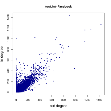
Figure 13: Scatter plot of node-wise out-degree and in-degree of Facebook wallpost graph.

The Facebook wall posts data was downloaded from http://konect.uni-koblenz.de/networks/facebook-wosn-wall and has been analyzed in [32]. Conversion of edge data to node-indexed in- and out-degree counts was done using the R-package igraph [6]. The data is a directed network representing posts by Facebook users to other users’ walls. Nodes are users and a directed edge represents one post from the user to the user whose wall is receiving the post. There are 46,952 users and 876,993 edges. We focus on out- and in-degree indexed by the nodes as $\{(Z_{1,i},Z_{2,i}):1\leqslant i\leqslant 46952\}$. Of course this data is not the result of iid replication but is rather node-indexed; however, for reasons still being investigated, conventional tools of heavy tail analysis seem quite effective on node-indexed network data. The scatter-plot of (out,in)-degrees in Figure 13 shows the expected strong asymptotic dependence between out- and in-degrees.

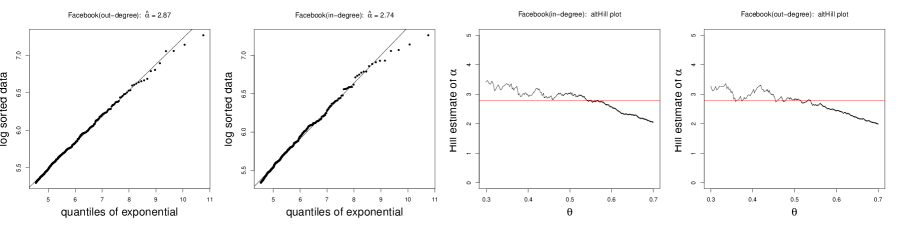
Figure 14: (Left) Marginal estimation of tail indices by QQ plot slope estimation and (right) altHill plotting for out- and in-degree. Horizontal lines are at height 2.8.

The plots in Figure 14 give the estimation of distribution tail indices for out- and in-degree. The slope estimator based on QQ-plots ([2; 22; 25]) gives approximately $\alpha=2.8$ for both out- and in-degree. Note this estimate is for the tail of the cumulative distribution functions and not, as is customary in network science, the index of the power law of the mass functions. The Hill estimator is ineffective and we have provided altHill plots ([25; 29; 13]).

Figure 15: Diamond plot restricted to the first quadrant for empirical angles thresholded using the 200 largest $L_{1}$ norms, along with the histogram and boxplot.

To get more information about the dependence structure, we construct a diamond plot using thresholding corresponding to the 200 largest $L_{1}$ norms of (out,in). The scatter plot in Figure 13 is less clear than for simulated data and shows points dispersed from the main cluster about the diagonal and so the estimates of the support of $\boldsymbol{\theta}$ in the diamond plot are not as evident as in Figure 15.

We estimate the support interval using the interquartile range and obtain $[.4479,.5305]=[\theta_{l},\theta_{u}]$. This corresponds to slopes $(a_{l},a_{u})=(\theta_{u}^{-1}-1,\theta_{l}^{-1}-1)=(.885,1.23).$ We also include a boxplot of the values of $\theta_{1}$ corresponding to the 200 largest values of the $L_{1}$ norm of (out,in).

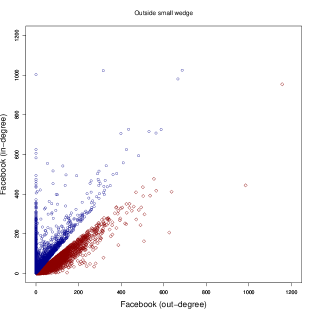
Figure 16: Points remaining after removal of $[\textsf{wedge}]$.

Having determined $[\textsf{wedge}]$, we remove it from the first quadrant and use the remaining points, illustrated in Figure 16, to seek hidden regular variation. Preliminary diagnostics use equations (3.6) and (3.7) corresponding to points above and below $[\textsf{wedge}]$ to estimate $\alpha_{0}$, the index of hidden regular variation. There are 12,089 points above $[\textsf{wedge}]$ in the region we refer to as $[>\textsf{wedge}]=\{(x,y):y>(1.23)x>0\}$ and 24,687 below in the region $[<\textsf{wedge}]=\{(x,y):0<y<(0.885)x\}.$

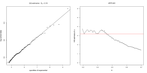
Figure 17: Facebook above $[\textsf{wedge}]$: QQ estimate is 3.2 for $k=100$ and altHill is 3.3; the red line is at height 3.3.

For the region $[<\textsf{wedge}]$, a combination of QQ and altHill plotting gives a stable region for various values of $k$, the number of upper order statistics, between 100-500 and a value of $\hat{\alpha}_{0}=2.8$, the tail index of $(0.885)Z_{1}-Z_{2}$ from (3.7), which is not measurably different from $\hat{\alpha}=2.8$ found for the marginal distributions of (out,in). This raises doubts about the presence of HRV in the region $[<\textsf{wedge}]$. For the region $[>\textsf{wedge}]$ we use as data $(Z_{2}-(1.23)Z_{1})_{+}$ and estimate $\hat{\alpha}_{0}\approx 3.2$. The QQ-estimate is 3.2 and altHill gives about 3.3; both estimates are greater than $\alpha=2.8$ so there is evidence of the existence of HRV in the region above $[\textsf{wedge}]$. The QQ and altHill plots for the region $[>\textsf{wedge}]$ are given in Figure 17. The evidence for HRV is further strengthened by excellent Hillish plots described in Section 3.6 applied to the generalized polar coordinates $(Z_{2}-(1.23)Z_{1},Z_{2}/Z_{1})$ as descibed in (3.8). Both Hillish plots in Figure 18 hug the horizontal line at height 1.

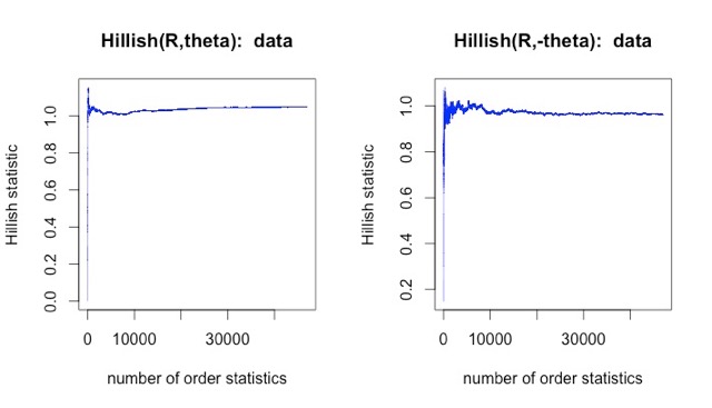
Figure 18: Hillish plots for generalized polar coordinates of points in $[>\textsf{wedge}]$.

The diamond plot in Figure 15 shows the presence of points on the line $x_{1}+x_{2}=1$ with small values of $\theta$, corresponding to two dimensional points in $[<\textsf{wedge}]$. Previously the estimation of the range of the angular measure of the primary regular variation discounted these points. However, the estimation of the tail index of the distance to $[\textsf{wedge}]$ being $2.8$, the same as the marginal distribution indices of (out,in), suggests an alternate model which lumps together $[\textsf{wedge}]\cup[<\textsf{wedge}]$ as the region of concentration for the limit measure $\nu(\cdot)$ of the primary regular variation in (2.4). So our alternate model is regular variation on $\mathbb{R}_{+}^{2}\setminus\{\boldsymbol{0}\}$ with index $2.8$ and limit measure which concentrates on $\{\boldsymbol{x}\in\mathbb{R}_{+}^{2}\setminus\{\boldsymbol{0}\}:x_{2}/x_{1}<1.23\}$ and hidden regular variation on $\mathbb{R}_{+}^{2}\setminus([\textsf{wedge}]\cup[<\textsf{wedge}])$ with index 3.3.

5.2 Exxon and Chevron returns.

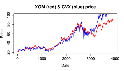
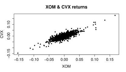
Figure 19: Stock prices and scatterplot of Chevron and Exxon returns.

For this example of financial returns, the state space is $\mathbb{R}^{2}\setminus\{\boldsymbol{0}\}$ and for the HRV property we could try deleting $[\textsf{wedge}_{+}]\subset\mathbb{R}_{+}^{2}$ in the first quadrant and $[\textsf{wedge}_{-}]\subset(-\infty,0)^{2}$ in the third quadrant. For illustration, we concentrate on deleting only a wedge from the first quadrant and seeking HRV with points above the upper boundary of $[\textsf{wedge}_{+}]$. This is done partly because there is no guarantee that HRV will hold globally. The data consists of closing daily prices of Exxon (XOM) and Chevron (CVX) from January 2, 1998 to August 9, 2013. For each variable we calculate daily returns for each company called (exxonr, chevronr). The length of the return vector is 3925. One expects strong dependence from two big companies engaged in similar economic activities and this is shown in the raw scatter plot of the variables in Figure 19.

The four tails of the variables ($\pm$exxonr, $\pm$chevronr) are quite similar. Based on analyses (not shown) using the QQ estimator, Hill and altHill plots, (eg. [22], [25, p. 101, 366]) we estimate

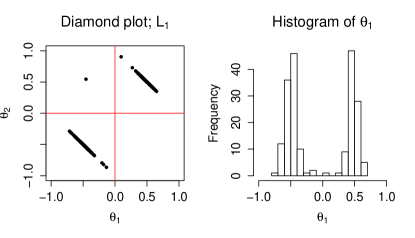
Figure 20: Diamond plot for 200 largest values under $L_{1}$ norm for (exxonr,chevronr) with histogram.

the marginal tail indices $\alpha=2.7$ in all four cases. Since the tails are estimated to have the same $\alpha$, we did not attempt to standardize the variables to $\alpha=1$ as is often done by either the power method or the ranks transform.

To understand the dependence structure of the variables (exxonr,chevronr), we make a diamond plot of the data. We do the mapping after thresholding the data at various values determined by $k$, the number of order statistics of the norms $|x_{1}|+|x_{2}|$. This is the two-tail empirical equivalent to (3.4) using the $L_{1}$ norm. After experimenting with thresholds, we settled on $k=200$ which in the first quadrant produced a range of $\theta_{1}=x_{1}/(x_{1}+x_{2})$ equal to $(.095,.649).$ We finalized our estimate of the support of the limit angular measure, by using the 10% and 90% quantiles of the values of $\theta_{1}$ as $(.393,.589)$. This corresponds to slope estimates for $[\textsf{wedge}]$ of $(\hat{a}_{l},\hat{a}_{u})=(.698,1.545)$. The strong asymptotic dependence among the marginals is evident from the diamond plot and histogram of $\theta_{1}$ in Figure (20). There is little evidence that a large positive change in one variable is accompanied by a large negative change in the other as shown by the lack of points in the second and fourth quadrants in Figure 20. There is no visual evidence supporting the hypothesis of full asymptotic dependence.

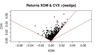
Figure 21: Points satisfying three conditions allowing computation of gpolar coordinates. Scanning counterclockwise, the first two rays define $[\textsf{wedge}_{+}]$ and the third ray is perpendicular to the upper boundary of $[\textsf{wedge}_{+}]$.

Remark 3.1 suggests verifying the necessary condition for HRV on $\mathbb{R}^{2}\setminus[\textsf{wedge}_{+}]$ by computing the tail index of what is essentially the distance of a point to $[\textsf{wedge}_{+}]$. We seek evidence of regular variation on $\mathbb{R}^{2}\setminus[\textsf{wedge}_{+}]$ by using points $\boldsymbol{x}$ of the return sample that satisfy,

1. $x_{2}>0$ (points above the horizontal axis);

2. $x_{2}-(1.545)x_{1}>0$ (points in the first or second quadrant above the ray $x_{2}=1.545x_{1},\,x_{1}>0$)

3. $x_{1}+1.545x_{2}>0$ (points in the first or second quadrant in the region bounded by the ray $x_{2}=1.545x_{1},\,x_{1}>0$ and the ray perpendicular to this ray emanating from the origin into the third quadrant). Points to the left of this perpendicular would be closer to $[\textsf{wedge}_{-}]$ rather than $[\textsf{wedge}_{+}]$ and are excluded.

There are 706 points satisfying the three conditions; we call these points oilReturns2013Gr. These are plotted in Figure 21. The angle between the two rays of biggest slope is 90 degrees.

We estimate the tail index $\alpha_{0}$ of the distance of points in oilReturns2013Gr to the boundary of $[\textsf{wedge}_{+}]$ to be greater than $\alpha=2.7$ using altHill, Hill and QQ plots. This corresponds to estimating the tail index of $Z_{2}-a_{u}Z_{1}$ as in (3.6). The plots are given next.

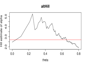
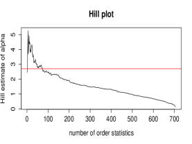
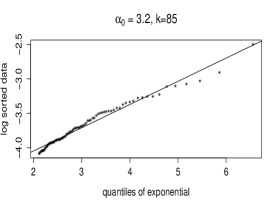
Figure 22: AltHill, Hill and QQ plots to estimate $\alpha_{0}$. The red horizontal lines are drawn at height $\alpha=2.7$.

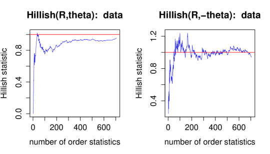
Figure 23: Hillish plots for generalized polar coordinates of points in oilReturns2013Gr.

More evidence for existence of HRV in the region corresponding to oilReturns2013Gr is provided by converting the data points in this region using the generalized polar coordinates suggested by (3.8). This produces the Hillish plots given in Figure 23. Both Figures 22 and 23 are encouraging.

6 Conclusions

Whenever the limit measure of multivariate regular variation concentrates on a cone smaller than the full state space, there is the potential for seeking hidden regular variation. This idea has been most often applied to the case of asymptotic independence where the limit measure concentrates on the axes. Here we have shown the idea is also applicable when the limit measure concentrates on the diagonal or a narrow cone such as $[\textsf{wedge}]$.

Without hidden regular variation, asymptotic independence causes analysts to miss risk contagion. Analogously, when the limit measure concentrates on the diagonal, analysis would estimate the probability of a risk region $\{(x,y):y-x>4\}$ to be zero when in fact, hidden regular variation would yield a small but non-zero probability. Our data analyses show potential for such estimation in strongly dependent data with heavy-tailed marginal distributions.

Without doubt, much work remains to be done on implementation. Both our network data which is node based and our returns data is nothing like independent replicated data. Also, our methods for estimating the support of the angular measure $S(\cdot)$ are primitive at best. Higher dimensional examples present increased visualization and estimation difficulties. None-the-less, we believe the worked out examples are useful and illustrate practical cases. Other examples exist and in particular we have analyzed Microsoft vs Dell returns with results similar to those found in Section 5.2.

7 Acknowledgements

We acknowledge with thanks the contribution in fall 2014 of Amy Willis who skilfully analyzed many financial data sets seeking examples of asymptotic full and strong asymptotic dependence. We are also grateful to Paul Embrechts who read an early draft and had many useful and encouraging comments. Two referees made many helpful and insightful comments.

B. Das was supported by MOE-2013-T2-1-158 and IDG31300110. B. Das also acknowledges hospitality from Cornell University during visits in June 2015 and January 2016. S. Resnick was supported by Army MURI grant W911NF-12-1-0385 to Cornell University.

References

- [1] P.L. Anderson and M.M. Meerschaert. Modeling river flows with heavy tails. Water Resources Research, 34(9):2271–2280, 1998.
- [2] J. Beirlant, P. Vynckier, and J. Teugels. Tail index estimation, Pareto quantile plots, and regression diagnostics. J. Amer. Statist. Assoc., 91(436):1659–1667, 1996.
- [3] N. H. Bingham, C. M. Goldie, and J. L. Teugels. Regular variation, volume 27 of Encyclopedia of Mathematics and its Applications. Cambridge University Press, Cambridge, 1989.
- [4] B. Bollobás, C. Borgs, J. Chayes, and O. Riordan. Directed scale-free graphs. In Proceedings of the Fourteenth Annual ACM-SIAM Symposium on Discrete Algorithms (Baltimore, 2003), pages 132–139, New York, 2003. ACM.
- [5] M. Crovella, A. Bestavros, and M.S. Taqqu. Heavy-tailed probability distributions in the world wide web. In M.S. Taqqu R. Adler, R. Feldman, editor, A Practical Guide to Heavy Tails: Statistical Techniques for Analysing Heavy Tailed Distributions. Birkhäuser, Boston, 1999.
- [6] G. Csardi and T. Nepusz. The igraph software package for complex network research. InterJournal, Complex Systems, 1695(5):1–9, 2006.
- [7] B. Das, P. Embrechts, and V. Fasen. Four theorems and a financial crisis. The International Journal of Approximate Reasoning, 54(6):701–716, 2013.
- [8] B. Das, A. Mitra, and S.I. Resnick. Living on the multidimensional edge: seeking hidden risks using regular variation. Advances in Applied Probability, 45(1):139–163, 2013.
- [9] B. Das and S.I. Resnick. Conditioning on an extreme component: Model consistency with regular variation on cones. Bernoulli, 17(1):226–252, 2011.
- [10] B. Das and S.I. Resnick. Detecting a conditional extreme value model. Extremes, 14(1):29–61, 2011.
- [11] B. Das and S.I. Resnick. Models with hidden regular variation: generation and detection. Stochastic Systems, 5:195–238 (electronic), 2015. http://www.i-journals.org/ssy/viewarticle.php?id=141.
- [12] L. de Haan and A. Ferreira. Extreme Value Theory: An Introduction. Springer-Verlag, New York, 2006.
- [13] H. Drees, L. de Haan, and S.I. Resnick. How to make a Hill plot. Ann. Statist., 28(1):254–274, 2000.
- [14] R.T. Durrett. Random Graph Dynamics. Cambridge Series in Statistical and Probabilistic Mathematics. Cambridge University Press, Cambridge, 2010.
- [15] P. Embrechts, C. Klüppelberg, and T. Mikosch. Modelling Extreme Events for Insurance and Finance. Springer-Verlag, Berlin, 1997.
- [16] J.E. Heffernan and S.I. Resnick. Hidden regular variation and the rank transform. Advances in Applied Probability, 37(2):393–414, 2005.
- [17] J.E. Heffernan and S.I. Resnick. Limit laws for random vectors with an extreme component. The Annals of Applied Probability, 17(2):537–571, 2007.
- [18] J.E. Heffernan and J.A. Tawn. A conditional approach for multivariate extreme values (with discussion). Journal of the Royal Statistical Society, Series B, 66(3):497–546, 2004.
- [19] H. Hult and F. Lindskog. On regular variation for infinitely divisible random vectors and additive processes. Adv. in Appl. Probab., 38(1):134–148, 2006.
- [20] H. Hult and F. Lindskog. Regular variation for measures on metric spaces. Publications de l’Institut Mathématique, Nouvelle Série, 80(94):121–140, 2006.
- [21] R. Ibragimov, D. Jaffee, and J. Walden. Diversification disasters. Journal of Financial Economics, 99(2):333–348, 2011.
- [22] M. Kratz and S.I. Resnick. The qq–estimator and heavy tails. Stochastic Models, 12:699–724, 1996.
- [23] F. Lindskog, S.I. Resnick, and J. Roy. Regularly varying measures on metric spaces: hidden regular variation and hidden jumps. Probability Surveys, 11:270–314, 2014.
- [24] S.I. Resnick. Hidden regular variation, second order regular variation and asymptotic independence. Extremes, 5(4):303–336, 2002.
- [25] S.I. Resnick. Heavy Tail Phenomena: Probabilistic and Statistical Modeling. Springer Series in Operations Research and Financial Engineering. Springer-Verlag, New York, 2007.
- [26] S.I. Resnick. Extreme Values, Regular Variation and Point Processes. Springer Series in Operations Research and Financial Engineering. Springer, New York, 2008. Reprint of the 1987 original.
- [27] S.I. Resnick. Multivariate regular variation on cones: application to extreme values, hidden regular variation and conditioned limit laws. Stochastics: An International Journal of Probability and Stochastic Processes, 80:269–298, 2008.
- [28] S.I. Resnick and G. Samorodnitsky. Tauberian theory for multivariate regularly varying distributions with application to preferential attachment networks. Extremes, 18(3):349–367, 2015.
- [29] S.I. Resnick and C. Stărică. Smoothing the Hill estimator. Adv. Applied Probab., 29:271–293, 1997.
- [30] G. Samorodnitsky, S. Resnick, D. Towsley, R. Davis, A. Willis, and P. Wan. Nonstandard regular variation of in-degree and out-degree in the preferential attachment model. Journal of Applied Probability, 53(1):146–161, March 2016. http://arxiv.org/pdf/1405.4882.pdf.
- [31] R.L. Smith. Statistics of extremes, with applications in environment, insurance and finance. In B. Finkenstadt and H. Rootzén, editors, SemStat: Seminaire Europeen de Statistique, Exteme Values in Finance, Telecommunications, and the Environment, pages 1–78. Chapman-Hall, London, 2003.
- [32] B. Viswanath, A. Mislove, M. Cha, and K.P. Gummadi. On the evolution of user interaction in facebook. In Proceedings of the 2nd ACM SIGCOMM Workshop on Social Networks (WOSN’09), August 2009.