Detrending Moving Average Algorithm:
Frequency Response and Scaling Performances

Abstract

The Detrending Moving Average (DMA) algorithm has been widely used in its several variants for characterizing long-range correlations of random signals and sets (one-dimensional sequences or high-dimensional arrays) either over time or space. In this paper, mainly based on analytical arguments, the scaling performances of the centered DMA, including higher-order ones, are investigated by means of a continuous time approximation and a frequency response approach. Our results are also confirmed by numerical tests. The study is carried out for higher-order DMA operating with moving average polynomials of different degree. In particular, detrending power degree, frequency response, asymptotic scaling, upper limit of the detectable scaling exponent and finite scale range behavior will be discussed.

I Introduction

To investigate whether the intensity of some relevant quantity is characterized by increasing or decreasing trends is a common goal to many research areas. In the simplest operational definition, trends are observed when a regression estimated over a data subset has a not negligible slope. For example in climatology, based on regular measurements from weather stations and satellite data, temperature trends are estimated both locally and globally Zhang2012 ; Tamazian2015 ; Yuan2015 ; Bromwich2013 . In finance and economics, technical rules and visualization tools based on moving average trends are under continuous investigation and improvement Lo ; Menkhoff ; Longstaff ; Daia . A main issue in the application of trend estimates is related to the assumption of the model describing the underlying evolution process (e.g. linear or exponential). Another critical aspect is the ability to distinguish whether the trend or other stochastic component embedded in a nonstationary time series arises from the intrinsic system dynamics or from external forcing drives (see e.g. Tamazian2015 ). Hence, the development of techniques (having the simultaneous ability of simulating trends and estimating long- and short-range correlations of stochastic data sets) and the assessment of their performances is of relevance to diverse scientific communities.

As a way to characterize nonstationary data with trend, the detrended fluctuation analysis (DFA)  Peng et al. (1994, 1995), and the detrending moving average (DMA) analysis  Alessio et al. (2002); Carbone et al. (2004); Arianos and Carbone (2007); Arianos et al. (2011) have been proposed to quantify long-range autocorrelations, multifractal features  GuPRE2010 ; GrechAPPB2005 ; BashanPhysA2008 ; MaPRE2010 ; Drozdz , cross-correlation  Podobnik ; ArianosJstat2009 and higher dimensional fractals GuPRE2006 ; CarbonePRE2007 ; TurkPRE2010 ; CarbonePRE2010 either in the time or in the space domain. According to the DFA, the time series is first divided in boxes of equal lengths, then trends are estimated as least-squares polynomial fitting of different orders $m$ in each non-overlapping and equally spaced box of length $n$. The DMA algorithm has been proposed as an alternative technique to quantify long-range correlations. In the frequency domain, the power spectral analysis is a well-established methodological framework Percival and Walden (1993); Hamilton (1994). By estimating the slope of the log-log plot of the power spectral density (PSD), a wide range of scaling behavior can be characterized. However, power spectral analysis may provide spurious estimates caused by the nonstationarity of time series, such as embedded trends and heterogeneous statistical properties.

Statistical performance (e.g. effects of nonstationarity, nonlinear filters and extreme data loss) of the DFA and DMA have been investigated by a number of comparative studies  Alvarez-Ramirez et al. (2005); Chianca et al. (2005); Hu et al. (2001); Chen et al. (2002); Xu et al. (2005); Chen et al. (2005). However, the performances of DMA, especially higher order ones and the relation between DMA and power spectral analysis have not been investigated. Therefore, the aim of this work is to understand such methodological features by an analytical approach based on the continuous time approximation and the single-frequency response of the DMA already adopted for DFA in KiyonoPRE2015 . Based on the exact calculation of the single-frequency response function under the continuous time approximation, the direct connection between DMA and power spectral analysis can be derived. Such relations are then exploited to derive a number of scaling performance features such as detrending power degree, frequency response, asymptotic behavior, upper limit of the scaling exponent and finite scale range behavior. The current work aims at providing clear mathematical reasoning for these properties and guiding principles to improve the detrending methodologies.

The organization of this paper is as follows. In Section II, the main computational steps of the DMA are briefly recalled together with a brief discussion highlighting the relevance of the high-order detrending methods and the limits of detrending performance in scaling analysis. In Section III and in the Appendixes, the analytical derivation of the performance characteristic mainly based on frequency response reasoning is reported. A comparison of the results obtained for the DMA to the DFA ones is offered all through the manuscript.

II Detrending Moving Average algorithm

As already stated above, the focus in this work is on the DMA operating with moving average polynomials of different degree. However, before entering the details of the present study, the basic elements of the DMA analysis will be summarized. The main ingredient of the DMA algorithm is the generalized variance $\sigma^{2}_{\rm DMA}(n)$ of the time series $\{y(i)\}_{i=1}^{N}$ with respect to the trend $\{\tilde{y}_{n}(i)\}$ at scale $n$:

$$\sigma^{2}_{\rm DMA}(n)=\frac{1}{N-n+1}\sum_{i}\Big{[}y(i)-\tilde{y}_{n}(i)\Big{]}^{2},$$ (1)

where $\tilde{y}_{n}(i)$ is defined as a time-dependent average function of $y(i)$. In the simplest case, called backward DMA, $\tilde{y}_{n}(i)$ can be estimated as the ordinary moving average:

$$\tilde{y}_{n}(i)=\frac{1}{n}\sum_{k=0}^{n-1}y(i-k),$$ (2)

and the range of the summation in Eq. (1) is from $n$ to $N$. For random walk-type processes with diffusive behavior, such as the fractional Brownian motion, the power-law increase of the root-mean square deviation $\sigma_{\rm DMA}(n)$ with the moving average window size $n$:

$$\sigma_{\rm DMA}(n)\sim n^{\alpha},$$ (3)

provides an estimate of the scaling exponent $\alpha$ and thus of the Hurst exponent $H$. For long-range correlated time series $\{x(i)\}_{i=1}^{N}$ with non-diffusive behavior, such as fractional Gaussian noise (fGn), the integrated series (cumulative sum), $y(i)=\sum_{j=1}^{i}x(j)$, as a sample path of a random walk driven by $\{x(i)\}$ is investigated and quantified in terms of the scaling exponent $\alpha$.

As a generalization of Eqs. (1) and (2), the high-order DMA (DMA_m) has been proposed where the trends $\{\tilde{y}_{n}(i)\}$ are defined in terms of moving average polynomials of degree $m$  Arianos et al. (2011). In this framework, the DMA algorithm with the conventional moving average given by Eq. (2) is referred to as the zeroth order DMA (DMA₀).

In the case of the centered DMA_m, the coefficients of the $m$th degree polynomials with moving average window over a range $[i-(n-1)/2,i+(n-1)/2]$, where $n$ is assumed to be an odd number, are given by:

$$\left[\begin{array}[]{c}\tilde{a}_{n,0}(i)\\ \tilde{a}_{n,1}(i)\\ \vdots\\ \tilde{a}_{n,m}(i)\\ \end{array}\right]=B_{m}^{-1}(i,n)\left[\begin{array}[]{c}\displaystyle\sum_{i^{\prime}=i-(n-1)/2}^{i+(n-1)/2}y(i^{\prime})\\ \displaystyle\sum_{i^{\prime}=i-(n-1)/2}^{i+(n-1)/2}{i^{\prime}}\,y(i^{\prime})\\ \vdots\\ \displaystyle\sum_{i^{\prime}=i-(n-1)/2}^{i+(n-1)/2}{(i^{\prime})}^{m}y(i^{\prime})\end{array}\right],$$ (4)

where $B_{m}^{-1}(i,n)$ is the inverse matrix of

$$B_{m}(i,n) = \sum_{{i^{\prime}}=i-(n-1)/2}^{i+(n-1)/2}\left[\begin{array}[]{cccc}1&{i^{\prime}}&\cdots&({i^{\prime}})^{m}\\ {i^{\prime}}&({i^{\prime}})^{2}&\cdots&({i^{\prime}})^{m+1}\\ \vdots&\vdots&\ddots&\vdots\\ ({i^{\prime}})^{m}&({i^{\prime}})^{m+1}&\cdots&({i^{\prime}})^{2m}\\ \end{array}\right].$$ (9)

Thus, the moving average polynomial of degree $m$ is expressed as:

$$\tilde{y}_{n,m}(i)=\tilde{a}_{n,0}\!\left(i\right)+\tilde{a}_{n,1}\!\left(i\right)\,i+\cdots+\tilde{a}_{n,m}\!\left(i\right)\,i^{m},$$ (11)

where $i=1+(n-1)/2,\cdots,N-(n-1)/2$ and the coefficients $\left\{\tilde{a}_{n,m}\right\}$ in Eq. (11) are not constant, as they in fact are dependent on $i$ (see also Fig. 1). To estimate $\sigma^{2}_{\rm DMA}(n)$ [Eq. (1)] in the centered DMA_m, the moving average polynomial $\left\{\tilde{y}_{n,m}(i)\right\}$ is used as the trend $\left\{\tilde{y}_{n}(i)\right\}$ and the range of summation in Eq. (1) is from $1+(n-1)/2$ to $N-(n-1)/2$. The current investigation is limited to even order centered DMA, infact the $2k$th and $(2k+1)$th order centered DMA, where $k$ is a nonnegative integer, have been proven to be equivalent in Arianos et al. (2011); PAPER2 .

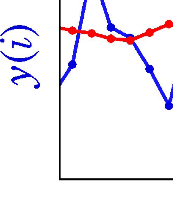
Figure 1: Illustration of the moving average polynomial of degree $m$ (bottom) for centered DMA_m [Eqs. (4) and (11)], where $n$ is equal to 11 for all the cases. (a) Zeroth order ($m=0$, corresponding to the conventional moving average); (b) first order ($m=1$); and (c) second order ($m=2$). In top three rows, the center point (red points) on each polynomial fit (black lines) in a local moving average window (gray shaded areas) is defined as the higher-order moving average point, and the moving average polynomial $\{\tilde{y}_{n,m}(i)\}$ is calculated by point-by-point sliding of the window. On the other hand, for the backward DMA (given by Eq. (2)), the far right point in the window is defined as the moving average reference point. Note that, in the centered DMA, $\{\tilde{y}_{n,0}(i)\}$ in DMA₀ (bottom left) and $\{\tilde{y}_{n,1}(i)\}$ in DMA₁ (bottom middle) are identical.

As an illustrative example in Fig. 2, the trends calculated by using the third order DFA (left panels) and the second order DMA (right panels) are shown. One can note that the DFA trend shows discontinuous jumps at the end points of each box. Conversely, the DMA trend exhibits seemingly continuous behavior. This is a crucial difference between DFA and DMA.

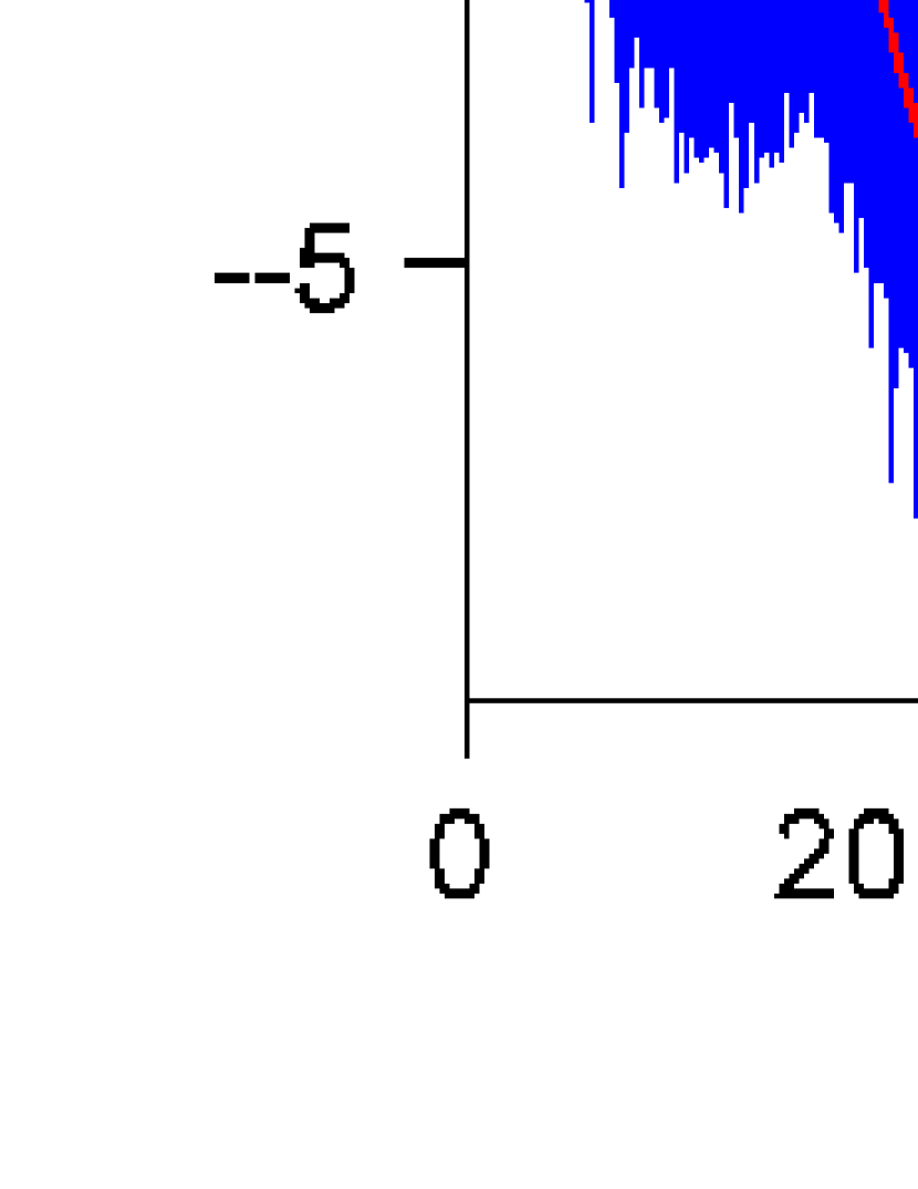
Figure 2: Illustration of trends estimated by the DFA₃ (left panels) and the centered DMA₂ (right panels). The box widths for the DFA₃ trend estimates are equal to 49 (top) and 99 (bottom). The moving average windows for the DMA₂ are equal to 49 (top) and 99 (bottom).

To date, the performance of the zeroth order DMA algorithm (DMA₀) has been extensively studied  Alvarez-Ramirez et al. (2005); Chianca et al. (2005); Hu et al. (2001); Chen et al. (2002); Xu et al. (2005); Chen et al. (2005). Conversely, the fundamental properties of the higher-order DMA (DMA_m with $m\geq 1$) have not been completely investigated  Arianos et al. (2011). To fill this knowledge gap and understand the methodological performances of DMA_m, we study the properties of the high-order DMA based on analytical arguments and numerical tests. Furthermore, the results of the study will be thoroughly compared to DFA. In the remainder of this section, based on preliminary numerical results, we provide an overview of the issues involved in the performance of the high-order DMA.

II.1 Importance of High-Order Detrending

When real-world long-range correlated series with nonstationary trends should be analyzed, high-order detrending is needed to detect the meaningful scaling exponents of the stochastic fluctuations embedded in the intrinsic or extrinsic trends. To illustrate this situation, let us consider the following case studies of artificially time series generated by:

(i)

the sum of a fGn with $H=0.3$ and a quadratic deterministic trend [Fig. 3 (top left)]

(ii)

the sum of a fGn with $H=0.3$ and a cubic stochastic trend [Fig. 3 (bottom left)] obtained as the interpolation of Gaussian generated points by a cubic spline.

In Fig. 3 (top and bottom right), the log-log plots of the centered DMA₀, DMA₂ and DFA₁, DFA₂, DFA₃ vs $n$ are respectively shown.

As one can note [Fig. 3 (top right)], the plots of the DMA₀ show spurious scaling behavior as suggested by the slope much steeper than $H=0.3$ at large values of $n$. The steep slope is due to the adverse effect of the deterministic quadratic trend component. Conversely, the DMA₂ plot shows a scaling behavior with the correct slope $H=0.3$ over the whole range of $n$, which demonstrates that the moving average polynomial of second degree $\{\tilde{y}_{n,2}(i)\}$ is not affected by the deterministic quadratic trend. Similar results have been found for the higher-order DFA as shown in Fig. 3 respectively for DFA₁, DFA₂ and DFA₃. In particular for the case (ii) [Fig. 3(bottom)], one can note that the upper boundary of the scaling range of DFA₃ (or DMA₂) is approximately one order larger than that of DFA₁ (or DMA₀). As a conclusion, the general result of the investigation is that higher-order DFA and DMA can reduce the adverse effect of the quadratic and cubic trend, by extending the scaling range towards higher values of $n$ [Fig. 3].

To date the detrending ability of the DMA with respect to embedded polynomial trends has not been analyzed and understood in depth. Therefore, in this paper, we will analytically show the detrending ability of DMA with respect to different trends and compare the performance with the DFA.

As a final remark, given the relevance of the above issues, it is convenient to introduce a figure of merit for scaling methods to remove a polynomial trend that we will refer to as Detrending Power Degree.

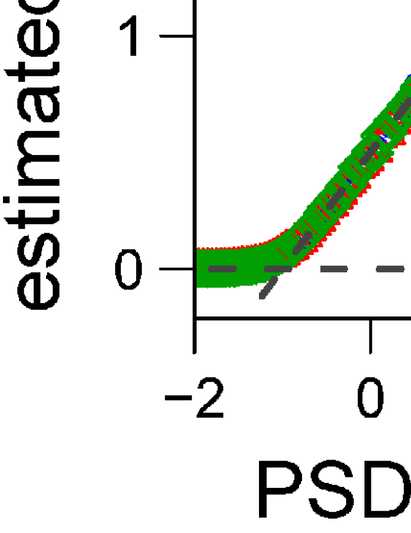
Figure 3: Scaling analysis of nonstationary time series with smooth trends. (Top) A sample time series generated by the sum of fractional Gaussian noise with $\alpha=0.3$ and a quadratic trend component. (Bottom) A sample time series generated by the sum of fractional Gaussian noise with $\alpha=0.3$ and a cubic spline trend in which 10 equally-spaced points with gaussian random numbers are interpolated by a cubic spline.

II.2 Upper limit of detectable scaling exponents

Next, the relationship between the upper limit of detectable scaling exponent $\alpha$ and the degree of the moving average polynomial is investigated. Though one can expect that upper limit would exist KiyonoPRE2015 , this aspect has not been systematically studied and thus will be analytically derived by using the single-frequency response function of DMA. Before illustrating the analytical results, the numerical results obtained for both DMA and DFA will be briefly discussed here.

Figure 4 (a) shows the scaling exponents $\alpha$ estimated by $m$th order DFA when sample time series with $1/f^{\beta}$ slope are analyzed. For the DFA, the relation $\alpha=(\beta+1)/2$ holds in a range $0<\alpha<m+1$, and the upper limit of detectable scaling exponent $\alpha$ is equal to $m+1$ KiyonoPRE2015 .

On the other hand, as shown in Fig. 4 (b), the upper limit of detectable scaling exponents of DMA₀ and DMA₂ are respectively two and four. Therefore, one can conclude that, both in DFA and DMA, higher-order detrending allow one to extend the upper limit of detectable scaling exponents.

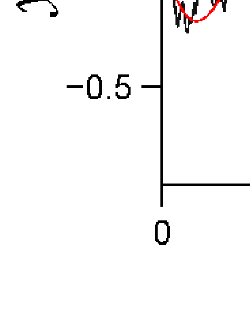
Figure 4: Scaling exponent $\alpha$ for a time series with power spectral density $1/f^{\beta}$ analyzed respectively by (a) first, second and third order DFA and (b) zeroth and second order DMA. Mean values of 30 samples are plotted.

III Analytical derivation of the DMA performance features

In this section, the methodological performances, discussed and illustrated by using the numerical results briefly illustrate in the previous section, will be analytically derived. It is worth noting that by using the approach proposed in this section, it would be possible to study properties of a wide class of random walk analysis including the several variants of the DMA.

III.1 Detrending Power Degree

Here, we study the Detrending Power Degree of the centered DMA, whose relevance for scaling analysis was discussed in subsection II.1. In particular, we will show that the DMA order $m$ which is defined by the degree of the moving average polynomial $\{\tilde{y}_{n,m}(i)\}$, is also related to the degree of the detectable polynomial trend embedded in the long-range correlated time series. More precisely, it will be shown that, when the integrated time series $y(i)$ is analyzed, the $m$th order DMA can correspondingly remove polynomial trend with degree $m$ in the original time series $x(i)$.

Let us consider the sum of two uncorrelated time series $x_{A}(i)$ and $x_{B}(i)$, the superposition law of the mean square deviation holds Shao :

$$\sigma^{2}_{\rm DMA}(n)_{A+B}=\sigma^{2}_{\rm DMA}(n)_{A}+\sigma^{2}_{\rm DMA}(n)_{B},$$ (12)

where $\sigma^{2}_{\rm DMA}(n)_{A}$, $\sigma^{2}_{\rm DMA}(n)_{B}$ and $\sigma^{2}_{\rm DMA}(n)_{A+B}$ denote the mean square deviation corresponding to $x_{A}(i)$, $x_{B}(i)$ and $x_{A}(i)+x_{B}(i)$, respectively. Therefore, if a time series is given by the sum of a fGn and a polynomial trend, the additive property of the mean square deviations holds. Therefore, the effect of the polynomial trend can be separated and investigated. We consider the $m$th order centered DMA, where $m$ is assumed to be a nonnegative even integer. To simplify the calculation, we assume a continuous function of $t$ over the range $-T/2\leq t\leq T/2$ with length (scale) $T$, and calculate the $m$th order moving average at $t=0$. Note that, by parallel translation, arbitrary situation of the polynomial trend in a moving average window can be described in the following form. Thus, without loss of generality, by considering only a single point at $t=0$, we can study the general properties of DMA. Let us consider a polynomial function with degree $q$, $x(t)=c_{0}+c_{1}t+\cdots+c_{q}t^{q}$, as the trend component in the original time series, and analyze its integrated function as:

$$y(t)=c_{0}t+\frac{c_{1}}{2}t^{2}+\cdots+\frac{c_{q}}{q+1}t^{q+1}=\sum_{k=0}^{q}\frac{c_{k}}{k+1}t^{k+1}.$$ (13)

To calculate the value of the moving average polynomial at $t=0$, one needs first to calculate the coefficients $\{a_{k}\}$ of the least-squares polynomial by minimizing

$$I\left(\{a_{k}\}\right)=\int_{-T/2}^{T/2}\!\left(\sum_{k=0}^{q}\frac{c_{k}}{k+1}t^{k+1}-\sum_{k=0}^{m}a_{k}t^{k}\right)^{2}\,dt.$$ (14)

Then, by using $\{a_{k}\}$ and substituting $t=0$ into the integrand in Eq. (14), the square deviation from the moving average polynomial at $t=0$ is given by $a_{0}^{2}$. Finally, as shown in the Appendix A, we obtain:

$$a_{0}^{2}=0\qquad{\rm for}\quad q\leq m\hskip 5.0pt,$$ (15)

which means that the moving average polynomial of degree $m$ coincides with $(q+1)$th degree polynomial trend $y(t)$ after integration. Thus, its generalized variance is equal to zero. In other words, if we evaluate the detrending power degree based on the order of the analyzed polynomial function $x(t)=\sum_{k=0}^{q}c_{k}\,t^{q}$, the detrending power degree of the centered DMA_m is equal to $m$. In contrast, the detrending power degree of $m$th order DFA is equal to $m-1$.

Analogously, for $q>m$, the square deviation from the polynomial trend takes a nonzero value. For instance, when $m=0$ and $q=1$, we get:

$$\sigma^{2}_{\rm DMA}(n)\approx\frac{c_{1}^{2}}{576}n^{4},$$ (16)

and, when $m=2$ and $q=3$, we get:

$$\sigma^{2}_{\rm DMA}(n)\approx\frac{9c_{3}^{2}}{5017600}n^{8}.$$ (17)

These results demonstrate that the polynomial trend with degree $q>m$ exhibits a spurious scaling behavior. Therefore, when the sum of a fractional Gaussian noise and a polynomial function with degree $q>m$ is analyzed by the centered DMA_m, a crossover in the plot of $\log\sigma_{\rm DMA}(n)$ vs $\log n$ appears according to the superposition law [Eq. (12)]. The numerical results plotted in Fig. 3 confirm the above findings.

III.2 Frequency Response

Here, by using the power spectral density of a fGn and the frequency response of DMA, we will investigate the properties of DMA when fractional Gaussian noises are analyzed.

It has been rigorously shown that the PSD of a fGn, increment process of a fractional Brownian motion with the Hurst exponent $H$, is given by KOU2004 ; Li and Lim (2006); Li (2009):

$$S(\omega)=\sigma^{2}\sin(H\pi)\Gamma(2H+1)|\omega|^{1-2H},$$ (18)

where $\omega$ is the angular frequency, $\sigma^{2}$ is the scale parameter of fGn, and $\Gamma$ is the gamma function.

To evaluate the frequency response of DMA, we first calculate the single-frequency response function under a continuous time approximation. The single-frequency response function provides an analytical approximation of the generalized variance when a single-frequency signal component having amplitude $A$ and frequency $f$ is analyzed. Note that, as given in Appendix B, it is possible to calculate the exact form of the single-frequency response function without the continuous time approximation. However, to simplify the calculation and to compare with the previous study of DFA KiyonoPRE2015 , we here use the continuous time approximation.

Let us thus consider the single frequency component, $x(t)=A\cos\left(2\pi ft+\theta\right)$, a continuous-time signal that after integration can be written as:

$$y(t)=\frac{A}{2\pi f}\sin\left(2\pi ft+\theta\right)\hskip 5.0pt,$$ (19)

where the constant integration term has been neglected. For the purpose of simplicity, the following calculation will be limited to the interval $\left[-T/2,T/2\right]$ of length $T$ corresponding to the scale $n$ in the discrete-time notation. To investigate the frequency response of the centered DMA, we estimate the square deviation at $t=0$ with respect to the moving average polynomial of degree $m$. To gain more insight into the DMA, it is valuable to note the difference in the calculation of the single-frequency response between DFA and DMA. In the previous study on DFA KiyonoPRE2015 , to calculate the single-frequency response function, the mean square deviation in a partitioned window (box) over $\left[-T/2,T/2\right]$ is assumed (see Eq. (12) in KiyonoPRE2015 ), because the statistical property of each window is identical. In contrast, in the case of DMA, the square deviation at only a single point ($t=0$) is assumed, because the statistical property at each point is identical. This may be an advantage of DMA, because the estimate of the mean square deviation in DMA has a better statistical symmetry than that in DFA.

In the centered DMA, the moving average polynomial is obtained by minimizing the following function:

$$I(\{a_{0},a_{1},\cdots,a_{m}\}) = \int_{-T/2}^{T/2}\!\left\{\frac{A}{2\pi f}\sin\left(2\pi ft+\theta\right)\right.$$ (20)

$$\left.-\sum_{i=0}^{m}a_{i}\,t^{i}\right\}^{2}\,dt\hskip 5.0pt.$$

where the coefficients $\{a_{i}\}$ of the polynomials are determined by solving the following equations:

$$\frac{\partial I(\{a_{i}\})}{\partial a_{j}}=0,$$ (21)

with $i,j=0,1,\cdots,m$.

The square deviation $\Phi^{2}$ with respect to the moving average polynomial at $t=0$ is given by

$$\Phi^{2}_{t=0}(T,f,A,\theta)=\left(\frac{A}{2\pi f}\sin\theta-a_{0}\right)^{2}\hskip 5.0pt,$$ (22)

that, by averaging the phase $\theta$ in over $[0,2\pi]$, could be approximated by:

$$\overline{\Phi}^{2}(T,f,A)=\frac{1}{2\pi}\int_{0}^{2\pi}\Phi^{2}_{t=0}(T,f,A,\theta)\,d\theta,$$ (23)

where we refer to $\overline{\Phi}^{2}$ as the single-frequency response function (more analytical details about $\overline{\Phi}^{2}$ are shown in the Appendix C). The square root of $\overline{\Phi}^{2}(T=n,f,A)$ can provide the analytical approximation of the $\sigma_{\rm DMA}(n)$ when a single-frequency component is analyzed. From the curves plotted in Fig. 5, one can note that the DMA₀ shows a single-frequency response similar to the DFA₁ and that the DMA₂ exhibits a single-frequency response similar to the DFA₃. The fine structure of the single-frequency response is informative of the fundamental properties and the performance of the DMA in the time and frequency domain.

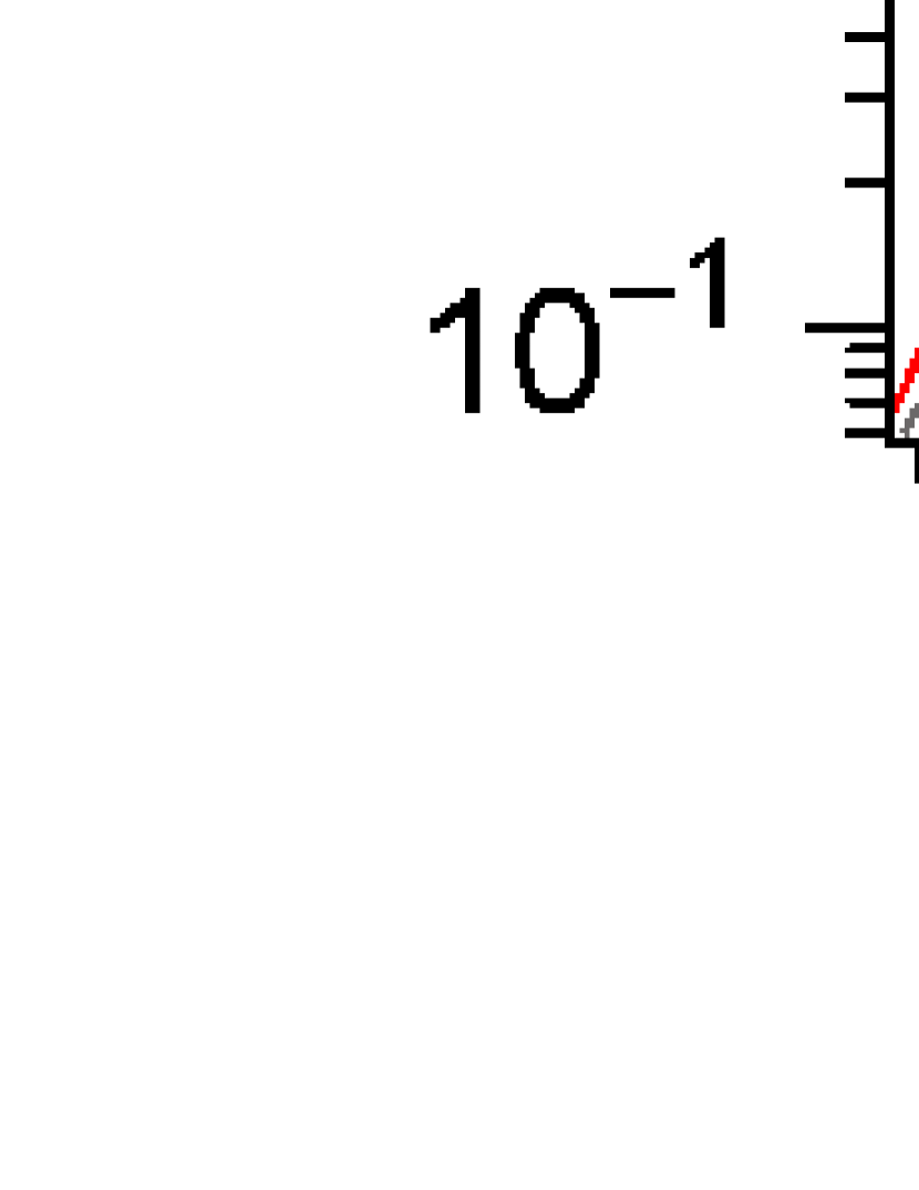
Figure 5: Single-frequency response functions $\overline{\Phi}^{2}(T,f,A)$ of zeroth and second order DMA, where $T$ is the window length, $A$ is the amplitude of a Fourier component with frequency $f$. (a) $\overline{\Phi}^{2}(T)$ versus scale $T$ with $f_{0}=10^{-3}$ and $A_{0}=1$. (c) $\overline{\Phi}^{2}(f)$ versus frequency $f$ with $T=10^{3}$ and $A_{0}=1$.

III.3 Asymptotic Scaling Behavior

Here, we will demonstrate that, on the basis of the single-frequency response calculated in subsection III.2, the PSD of a linear stochastic process can be converted into the root mean square deviation $\sigma_{\rm DMA}(n)$.

If the amplitude spectrum $\{A(f_{k})\}$, where $f_{k}$ is the frequency of $k$th harmonic component, is known, the single-frequency response function $\overline{\Phi}^{2}$ provides an estimate of $\sigma_{\rm DMA}(n)$ as follows:

$$\sigma_{\rm DMA}(n)=\left[\sum_{k=1}^{\lfloor N/2\rfloor}\!c(f_{k})\,\overline{\Phi}^{2}(n,f_{k},A(f_{k}))\right]^{1/2}\hskip 5.0pt,$$ (24)

where $c(f_{k})$ describes the effect of discrete time sampling:

$$c(f)=\frac{(\pi f)^{2}}{\sin^{2}(\pi f)}\hskip 5.0pt.$$ (25)

(see Ref. KiyonoPRE2015 for a detailed derivation of Eqs. (24) and (25)).

Furthermore, by using Eqs. (18) and (24), the scale dependence of $\sigma_{\rm DMA}(n)$ for fGn can be analytically estimated. As a representative example, we consider the asymptotic behavior of the DMA₂. When $n\ll 1/f$, the single-frequency response function $\overline{\Phi}^{2}$ [Eq. (23)] of DMA₂ can be expanded as:

$$\overline{\Phi}^{2}(n,f,A)={C_{1}A^{2}f^{6}n^{8}}+O\left(n^{10}\right),$$ (26)

with the constant $C_{1}=\pi^{6}/627200$. On the other hand, by taking the limit $n\to\infty$, we obtain

$$\lim_{n\to\infty}\overline{\Phi}^{2}(n,f,A)=\frac{C_{2}A^{2}}{f^{2}}.$$ (27)

with the constant $C_{2}=(8\pi^{2})^{-1}$. Based on Eqs. (26) and (27), $\overline{\Phi}^{2}(n,f,A)$ can be separated in two branches by:

$$\overline{\Phi}^{2}(n,f,A)\approx\left\{\begin{array}[]{ll}\displaystyle{C_{1}A^{2}f^{6}n^{8}}&\ {\rm for\ }n<\displaystyle\frac{f_{c}}{f}\\ \\ \displaystyle\frac{C_{2}A^{2}}{f^{2}}&\ {\rm for\ }n\geq\displaystyle\frac{f_{c}}{f}\end{array}\right.,$$ (28)

where $f_{c}=\frac{280^{1/4}}{\pi}$. If the power spectral density of a discrete sample of fGn is a $1/f$-sloped function:

$$S_{x}(f)=\frac{A_{0}^{2}}{f^{\beta}}$$ (29)

for $f\leq 1/2$, $\sigma_{\rm DMA}(n)$ can be estimated by assuming Eq. (28) and $c(f)\approx 1$ as

$$\sigma_{\rm DMA}^{2}(n) \sim \int_{0}^{1/2}\!\left.\overline{\Phi}^{2}\left(n,f,A\right)\right|_{A^{2}=A_{0}^{2}/f^{\beta}}\,df$$ (30)

$$\approx C_{1}\int_{0}^{f_{c}/n}\!f^{6}n^{8}\left(A_{0}^{2}\,f^{-\beta}\right)\,df+C_{2}\int_{f_{c}/n}^{1/2}\!\frac{1}{f^{2}}A_{0}^{2}f^{-\beta}\,df$$

$$= \left(C_{1}\frac{f_{c}^{7-\beta}}{7-\beta}+C_{2}\frac{f_{c}^{-\beta-1}}{\beta+1}\right)n^{\beta+1}-C_{2}\frac{2^{\beta+1}}{\beta+1}$$

where it is assumed $\beta<7$. For $n\gg 1$ and $-1<\beta<7$, the first term of Eq. (30) is dominant, thus it results:

$$\sigma_{\rm DMA}^{2}(n)\sim n^{\beta+1}.$$ (31)

which implies the following relationship:

$$\alpha=\frac{\beta+1}{2}\hskip 5.0pt.$$ (32)

Moreover since $\beta=2H-1$ for fGn, it turns out that $\alpha$ coincides asymptotically with $H$ of fGn. By using the same approach, analogous asymptotic laws can be derived for the high-order DMA_m.

III.4 Upper limit of detectable scaling exponent

The power-law tail structure of $\overline{\Phi}^{2}(n,f,A)\sim f^{\gamma-2}\,n^{\gamma}$ for $n\ll 1/f$ determines the upper limit of the detectable scaling exponent $\alpha$ given by $\alpha<\gamma/2$. If $\alpha>\gamma/2$, namely $\gamma-\beta-1<0$, the $\sigma_{\rm DMA}(n)$ can be evaluated as:

$$\sigma^{2}_{\rm DMA}(n) \sim \int_{0}^{f_{c}/n}\!f^{\gamma-2}n^{\gamma}\left(A_{0}^{2}\,f^{-\beta}\right)\,df$$ (33)

$$= \left(A_{0}^{2}\left[\frac{f^{\gamma-\beta-1}}{\gamma-\beta-1}\right]_{f=0}^{f_{c}/n}\right)n^{\gamma}$$

$$\approx \left(A_{0}^{2}\left[\frac{f^{\gamma-\beta-1}}{\gamma-\beta-1}\right]_{f=0}^{\epsilon}\right)n^{\gamma}$$

$$\sim n^{\gamma},$$

where $0<\epsilon\ll f_{c}/n$ is chosen such that:

$$\left[\frac{f^{\gamma-\beta-1}}{\gamma-\beta-1}\right]_{f=\epsilon}^{f_{c}/n}\ll\left[\frac{f^{\gamma-\beta-1}}{\gamma-\beta-1}\right]_{f=0}^{\epsilon}.$$

Thus, the estimated scaling exponent is independent of $\beta$, and given by $\alpha=\gamma/2$.

For $n\ll 1/f$, the single-frequency response of the DMA₀, DMA₂ and DMA₄ can be expanded in power of $n$ respectively as $\overline{\Phi}^{2}(n,f,A)\sim f^{2}n^{4}$, $\sim f^{6}n^{8}$, $\sim f^{10}n^{12}$, respectively (see Appendix C). Therefore, the scaling exponents $\alpha$ detectable by these methods are bounded by $2$, $4$ and $6$, respectively. Finally, one can conjecture that the upper limit of the detectable scaling exponent $\alpha$ by $2k$th order centered DMA, where $k$ is a nonnegative integer, would be $2k+2$.

III.5 Finite scale range behavior

The asymptotic behavior of the DMA when sample series of fGn are analyzed has been discussed on the basis of the single-frequency response function. In many practical situations, it is also important to understand the finite-range scale-dependence of $\sigma_{\rm DMA}(n)$. This issue will thus be investigated in this subsection.

By using Eqs. (18) and (24), the scale dependence of $\sigma_{\rm DMA}(n)$ can be calculated for fGn. As shown in Fig. 6 (solid lines), the predictions based on the analytical arguments are in good agreement with the numerical estimates obtained by the Monte Carlo approach. Through the analytical approach based on the single-frequency response function, we can precisely characterize the scaling behavior of fGn when analyzed by DMA. In Fig. 7, the scale dependence of $\sigma_{\rm DMA}(n)$ and its local slope are shown together with results obtained for DFA. The asymptotic convergence of the slope to the true value of $\alpha$ is very slow when $\alpha\approx 0$, as shown in Fig. 7(a). The local slopes at values of the scales $\log_{10}n<1.5$ show oscillating behavior for DMA, which results from the oscillation seen in the single-frequency response of DMA [Fig. 5(a)]. It is worthy of note that it would be very difficult to observe such fine structure of the $\sigma_{\rm DMA}(n)$ by using the Monte Carlo-based approach.

By the similarity of the single-frequency response functions of centered DMA_m and DFA_m+1 (see Fig. (5)), both methods show the similar finite scale range behavior in scales $\log_{10}n>1.5$.

Figure 6: Scale dependence of the root mean square deviation from trend, $\sigma_{\rm DMA}(n)$ with order of the moving average polynomials equal to zero and two, obtained by Monte Calro (circles) and analytical (solid lines) approach. Artificially generated time series with given scaling exponent $\alpha$ are used for the numerical tests.

Figure 7: Scale dependence of $\sigma_{\rm DMA}(n)$ and its local slope. $\sigma_{\rm DMA}(n)$ is analytically evaluated based on the single-frequency response function.

IV Conclusion

We studied methodological properties of high order centered DMA and on the basis of analytical arguments and numerical tests, we have demonstrated the following facts:

• $m$th order centered DMA can remove up to $m$th degree polynomial trend in the original time series before integration.

• The single-frequency response functions of DMA₀ and DMA₂ have similar structure of DFA₁ and DFA₃, respectively.

• The scaling exponent $\alpha$ estimated by centered DMA coincides asymptotically with the Hurst exponent $H$

• The upper limit of the detectable scaling exponent $\alpha$ by $m$th order centered DMA is $m+2$

It has been shown in Alvarez-Ramirez et al. (2005) that the detrending procedure in DFA is based on discontinuous polynomial fitting, which involves a nonlinear high-pass filter. Because of this nonlinearity, well established linear analysis methods, such as the frequency response based on frequency domain analysis, cannot be used on the DFA to investigate its methodological properties. To overcome this difficulty, a method based on the single-frequency response was recently proposed KiyonoPRE2015 . According to this method, the single-frequency response function is calculated through the analysis of a single-frequency component in the time domain, and can help to gain deeper insight into the performance of DFA including higher order cases KiyonoPRE2015 . In this paper, this approach has been applied to the investigation of DMA methodology. Our results have demonstrated that the performance of $m$th order centered DMA, where $m$ is a nonnegative even integer, is very well comparable with that of $(m+1)$th order DFA. It has been demonstrated that the zeroth order centered DMA has a good performance to characterize long-range correlation and fractal scaling behavior Alvarez-Ramirez et al. (2005); Shao2012 . In practical applications to real-world time series, the higher detrending power degree would be very important to improve estimation accuracy and to validate the observed scaling behavior Kantelhardt et al. (2001); Bashan et al. (2008). Hence, our results would facilitate further application of higher order DMA.

Appendix A Derivation of Eq. (15)

To obtain the least-squares polynomial by minimizing Eq. (14), we solve the following equations:

$$\frac{\partial I(\{a_{i}\})}{\partial a_{j}}=0,$$ (34)

where $i,j=0,1,\cdots,m$. When $j$ is even ($j=0,2,\cdots,m$), we get

$$\left[\begin{array}[]{cccc}\rho_{0}&\rho_{2}&\cdots&\rho_{m}\\ \rho_{2}&\rho_{4}&\cdots&\rho_{m+2}\\ \rho_{4}&\rho_{6}&\cdots&\rho_{m+4}\\ \vdots&\vdots&&\vdots\\ \rho_{m}&\rho_{m+2}&\cdots&\rho_{2m}\\ \end{array}\right]\left[\begin{array}[]{c}a_{0}\\ a_{2}-\frac{c_{1}}{2}\\ a_{4}-\frac{c_{3}}{4}\\ \vdots\\ a_{m}-\frac{c_{m-1}}{m}\\ \end{array}\right]=\left[\begin{array}[]{c}0\\ 0\\ 0\\ \vdots\\ 0\end{array}\right],$$ (35)

where

$$\rho_{k}=2\int_{0}^{T/2}\!\!t^{k}\,dt=\frac{2^{-k}}{k+1}T^{k+1}.$$ (36)

Because a unique solution should exist in the case of the least squares method, we obtain

$$a_{0} = 0$$ (37)

$$a_{2k} = \frac{c_{2k-1}}{2k}\qquad{\rm for}\quad k=1,2,\cdots m/2.$$ (38)

Appendix B Exact calculation of the single-frequency response for discrete time series

To obtain the single-frequency response function, we have used a continuous time approximation. As we demonstrated in this paper, the single-frequency response function calculated under this assumption can help to gain deeper insight into the performance of DMA. However, it is also possible to calculate the exact form of the single-frequency response when discrete time series is analyzed, although the amount of calculation is somewhat large. Here we provide some exact formulas of the single-frequency response function.

To obtain the single-frequency response function at scale $n=2n^{\prime}+1$ for centered DMA, let us consider discrete-time series $\{x(i)\}$,

$$x(i)=A\cos\left(2\pi fi+\theta\right),$$ (39)

in the range $[-n^{\prime},n^{\prime}]$. In this case, the integrated series is given by

$$y(i) = \sum_{j=-n^{\prime}}^{i}x(i)$$

$$= \frac{A\sin\{\pi f(i+n+1)\}\sin\{\pi f(i-n)+\theta\}}{\sin(\pi f)}.$$

To calculate the moving average polynomial at $i=0$, we first obtain coefficients $\{a_{k}\}$ of the least-squares polynomial with degree $m$ by minimizing

$$I\left(\{a_{j}\}\right)=\sum_{i=-n^{\prime}}^{n^{\prime}}\left(y(i)-\sum_{k=0}^{m}a_{k}i^{k}\right)^{2}.$$ (41)

After the determination of $\{a_{k}\}$, the mean-square deviation at $i=0$ is given by

$$\Phi_{\rm d}^{2}(n,f,A,\theta)=\left(y(i)-\sum_{k=0}^{m}a_{k}i^{k}\right)^{2}.$$ (42)

By averaging the phase $\theta$ in this equation over $[0,2\pi]$, we finally obtain the single-frequency response function $\overline{\Phi}_{\rm d}^{2}(n,f,A)$ for the discrete-time series $\{x(i)\}$.

For instance, in the zeroth order case, the exact form of the single-frequency response function is given by:

$$\overline{\Phi}_{\rm d}^{2}(n,f,A) = \frac{A^{2}}{16(2n+1)^{2}\sin^{4}(\pi f)}\Big{[}4n^{2}+4n+2-(2n+1)^{2}\cos(2\pi f)$$

$$+(4n+2)\cos(2\pi f(n+1))-(4n+2)\cos(2\pi fn)-\cos(2\pi f(2n+1))\Big{]},$$

and in the second order case, by

$$\overline{\Phi}_{\rm d}^{2}(n,f,A) = \frac{A^{2}}{128(2n+1)^{2}\left(4n^{2}+4n-3\right)^{2}\sin^{8}(\pi f)}\Big{[}3\left(8n^{3}+12n^{2}-2n-3\right)\sin(\pi f)$$ (44)

$$+\left(-8n^{3}-12n^{2}+2n+3\right)\sin(3\pi f)+3\left(2n^{2}+7n+6\right)\sin(\pi f(1-2n))$$

$$+3(2n-1)((2n+3)\sin(\pi f(2n+1))-(n-1)\sin(\pi f(2n+3)))\Big{]}^{2}.$$

The functional forms of the single-frequency response functions for discrete-time and continuous-time cases are illustrated in Fig. 8, where one can note that, except for differences at very small scales, the single frequency response function calculated under the continuous-time approximation in Section III is in excellent agreement with its exact result.

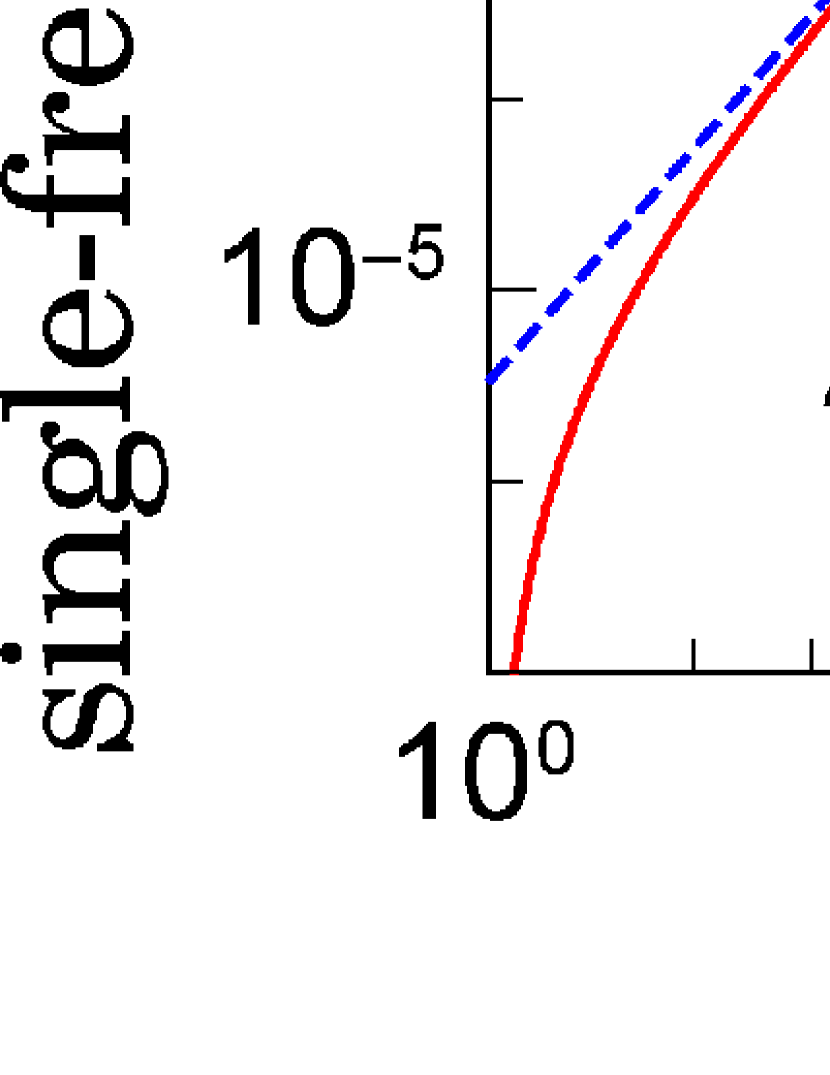
Figure 8: The single-frequency response function of $m$th order centered DMA for $A=1$, and $f=0.01$.

Appendix C Single-frequency response function of DMA

Zeroth-order and first-order centered DMA

($m=0,1$)

$$a_{0} = \frac{A\sin\theta\,\sin(\pi fT)}{2\pi^{2}f^{2}T}$$ (45)

$$\overline{\Phi}^{2}(T,f,A) = \frac{A^{2}\left\{\sin(\pi fT)-\pi fT\right\}^{2}}{8\pi^{4}f^{4}T^{2}}$$

$$= \frac{\pi^{2}A^{2}f^{2}T^{4}}{288}+O\left(T^{6}\right)\quad(T\ll 1/f)$$

Second-order and Third-order centered DMA

($m=2,3$)

$$a_{0} = -\frac{3A\sin\theta\,\left\{\pi^{2}f^{2}T^{2}\sin(\pi fT)-5\sin(\pi fT)+5\pi fT\cos(\pi fT)\right\}}{4\pi^{4}f^{4}T^{3}}$$ (48)

$$\overline{\Phi}^{2}(T,f,A) = \frac{A^{2}\left\{2\pi^{3}f^{3}T^{3}+3\left(\pi^{2}f^{2}T^{2}-5\right)\sin(\pi fT)+15\pi fT\cos(\pi fT)\right\}^{2}}{32\pi^{8}f^{8}T^{6}}$$ (49)

$$= \frac{\pi^{6}A^{2}f^{6}T^{8}}{627200}+O\left(T^{10}\right)\quad(T\ll 1/f)$$ (50)

Fourth-order and Fifth-order centered DMA

($m=4,5$)

$$a_{0} = \frac{15A\sin(\theta)}{16\pi^{6}f^{6}T^{5}}\left\{\pi^{4}f^{4}T^{4}\sin(\pi fT)+14\pi^{3}f^{3}T^{3}\cos(\pi fT)-77\pi^{2}f^{2}T^{2}\sin(\pi fT)+189\sin(\pi fT)\right.$$

$$\left.-189\pi fT\cos(\pi fT)\right\}$$

$$\overline{\Phi}^{2}(T,f,A) = \frac{A^{2}}{512\pi^{12}f^{12}T^{10}}\left(-8\pi^{5}f^{5}T^{5}+105\pi fT\left(2\pi^{2}f^{2}T^{2}-27\right)\cos(\pi fT)\right.$$ (52)

$$\left.+15\left(\pi^{4}f^{4}T^{4}-77\pi^{2}f^{2}T^{2}+189\right)\sin(\pi fT)\right)^{2}$$

$$= \frac{\pi^{10}A^{2}f^{10}T^{12}}{8851949568}+O\left(T^{14}\right)\quad(T\ll 1/f)$$ (53)

References

- (1) X. Zhang, and J.A. Church, Geophys. Res. Lett., 39, L21701, (2012).
- (2) A. Tamazian, J. Ludescher, A. Bunde, Phys. Rev. E, 91, 3 (2015).
- (3) N. Yuan, M. Ding, Y. Huang, Z. Fu, E. Xoplaki, and J. Luterbacher, J. Climate, 28, 5922, 934 (2015).
- (4) D. H. Bromwich, et al. Nature Geosci. 6, 139-45 (2013).
- (5) A.W. Lo, H. Mamaysky and J. Wang J. of Finance 55 1705 (2000).
- (6) L. Menkhoff, Journal of Banking & Finance 34 2573 (2010).
- (7) F.A. Longstaff and E.S. Schwartz, Rev. Financ. Stud. 14 113 (2001). Valuing American options by simulation: a simple least-squares approach
- (8) M. Dai, P. Li, and J.E. Zhang, J. of Econ. Dyn. Control, 34, 542 (2010).
- Peng et al. (1994) C.-K. Peng, S. V. Buldyrev, S. Havlin, M. Simons, H. E. Stanley, and A. L. Goldberger, Phys. Rev. E 49, 1685 (1994).
- Peng et al. (1995) C.-K. Peng, S. Havlin, H. E. Stanley, and A. L. Goldberger, Chaos 5, 82 (1995).
- Alessio et al. (2002) E. Alessio, A. Carbone, G. Castelli, and V. Frappietro, The European Physical Journal B 27, 197 (2002).
- Carbone et al. (2004) A. Carbone, G. Castelli, and H. Stanley, Phys. Rev. E 69, 026105 (2004).
- Arianos and Carbone (2007) S. Arianos and A. Carbone, Physica A 382, 9 (2007).
- Arianos et al. (2011) S. Arianos, A. Carbone, and C. Türk, Phys. Rev. E 84, 046113 (2011).
- (15) G.F. Gu and W.X. Zhou, Phys. Rev. E 82, 011136 (2010).
- (16) D. Grech and Z. Mazur, Acta Phys. Pol. B 36, 2403 (2005).
- (17) A. Bashan, R. Bartsch, J.W. Kantelhardt and S. Havlin, Physica A 387, 5080 (2008).
- (18) Q.D.Y Ma et al. Phys. Rev. E 81, 031101 (2010).
- (19) S. Drozdz, J. Kwapien, P. Oswiecimka and R. Rak, EPL 88, 60003 (2009).
- (20) S. Arianos and A. Carbone, J. Stat. Mech: Th. & Exp. P03037 (2009).
- (21) B. Podobnik and H.E. Stanley, Phys. Rev. Lett. 100, 084102 (2009).
- (22) G.F. Gu and W.X. Zhou, Phys. Rev. E 74, 061104 (2006).
- (23) A. Carbone, Phys. Rev. E 76, 056703 (2007).
- (24) C. Türk, A. Carbone and B.M. Chiaia, Phys. Rev. E 81, 026706 (2010).
- (25) A. Carbone, B.M. Chiaia, B. Frigo and C. Türk, Phys. Rev. E 82, 036103 (2010).
- Percival and Walden (1993) D. B. Percival and A. T. Walden, Spectral analysis for physical applications (Cambridge University Press, 1993).
- Hamilton (1994) J. D. Hamilton, Time series analysis, vol. 2 (Princeton university press Princeton, 1994).
- Alvarez-Ramirez et al. (2005) J. Alvarez-Ramirez, E. Rodriguez, and J. C. Echeverría, Physica A: Statistical Mechanics and its Applications 354, 199 (2005).
- Chianca et al. (2005) C. Chianca, A. Ticona, and T. Penna, Physica A: Statistical Mechanics and its Applications 357, 447 (2005).
- Hu et al. (2001) K. Hu, P. C. Ivanov, Z. Chen, P. Carpena, and H. E. Stanley, Phys. Rev. E 64, 011114 (2001).
- Chen et al. (2002) Z. Chen, P. C. Ivanov, K. Hu, and H. E. Stanley, Phys. Rev. E 65, 041107 (2002).
- Xu et al. (2005) L. Xu, P. C. Ivanov, K. Hu, Z. Chen, A. Carbone, and H. E. Stanley, Phys. Rev. E 71, 051101 (2005).
- Chen et al. (2005) Z. Chen, K. Hu, P. Carpena, P. Bernaola-Galvan, H. E. Stanley, and P. C. Ivanov, Phys. Rev. E 71, 011104 (2005).
- (34) Y.-H. Shao, G.-F. Gu, Z.-Q. Jiang, W.-X. Zhou and D. Sornette, Sci. Rep. 2, 835 (2012)
- (35) K. Kiyono, Phys. Rev. E 92 (4), 042925 (2015).
- (36) Y. Tsujimoto, Y. Miki, S. Shimatani and K. Kiyono, in preparation.
- (37) S.C. Kou and X. Sunney Xie, Phys. Rev. Lett.,93, 180603 (2004).
- Li and Lim (2006) M. Li and S. Lim, Fluct. Noise Lett. 6, C33 (2006).
- Li (2009) M. Li, Math. Probl. in Eng. 2010 (2009).
- (40) Y.-H. Shao, G.-F. Gu, Z.-Q. Jiang, W.-X. Zhou, Fractal 23, 1550034 (2015).
- Kantelhardt et al. (2001) J. W. Kantelhardt, E. Koscielny-Bunde, H. H. Rego, S. Havlin, and A. Bunde, Physica A: Statistical Mechanics and its Applications 295, 441 (2001).
- Bashan et al. (2008) A. Bashan, R. Bartsch, J. W. Kantelhardt, and S. Havlin, Physica A: Statistical Mechanics and its Applications 387, 5080 (2008).