Computing with Quasiseparable Matrices

Abstract

The class of quasiseparable matrices is defined by a pair of bounds, called the quasiseparable orders, on the ranks of the sub-matrices entirely located in their strictly lower and upper triangular parts. These arise naturally in applications, as e.g. the inverse of band matrices, and are widely used for they admit structured representations allowing to compute with them in time linear in the dimension. We show, in this paper, the connection between the notion of quasiseparability and the rank profile matrix invariant, presented in [Dumas & al. ISSAC’15]. This allows us to propose an algorithm computing the quasiseparable orders $(r_{L},r_{U})$ in time $O(n^{2}s^{\omega-2})$ where $s=\max(r_{L},r_{U})$ and $\omega$ the exponent of matrix multiplication. We then present two new structured representations, a binary tree of PLUQ decompositions, and the Bruhat generator, using respectively $O(ns\log\frac{n}{s})$ and $O(ns)$ field elements instead of $O(ns^{2})$ for the classical generator and $O(ns\log n)$ for the hierarchically semiseparable representations. We present algorithms computing these representations in time $O(n^{2}s^{\omega-2})$. These representations allow a matrix-vector product in time linear in the size of their representation. Lastly we show how to multiply two such structured matrices in time $O(n^{2}s^{\omega-2})$.

1 Introduction

The inverse of a tridiagonal matrix, when it exists, is a dense matrix with the property that all sub-matrices entirely below or above its diagonal have rank at most one. This property and many generalizations of it, defining the semiseparable and quasiseparable matrices, have been extensively studied over the past 80 years. We refer to [16] and [17] for a broad bibliographic overview on the topic. In this paper, we will focus on the class of quasiseparable matrices, introduced in [8]:

Definition 1

An $n\times n$ matrix $\mathsf{M}$ is $(r_{L},r_{U})$-quasiseparable if its strictly lower and upper triangular parts satisfy the following low rank structure: for all $1\leq k\leq n-1$,

$$\text{rank}(\mathsf{M}_{k+1..n,1..k}) \leq r_{L},$$ (1)

$$\text{rank}(\mathsf{M}_{1..k,k+1..n}) \leq r_{U}.$$ (2)

The values $r_{L}$ and $r_{U}$ define the quasiseparable orders of $\mathsf{M}$.

Quasiseparable matrices can be represented with fewer than $n^{2}$ coefficients, using a structured representation, called a generator. The most commonly used generator [8, 16, 17, 9, 1] for a matrix $\mathsf{M}$, consists of $(n-1)$ pairs of vectors $p(i),q(i)$ of size $r_{L}$, $(n-1)$ pairs of vectors $g(i),h(i)$ of size $r_{U}$, $n-1$ matrices $a(i)$ of dimension $r_{L}\times r_{L}$, and $n-1$ matrices $b(i)$ of dimension $r_{U}\times r_{U}$ such that

$$\mathsf{M}_{i,j}=\left\{\begin{array}[]{ll}p(i)^{T}\mathsf{a}^{>}_{ij}q(j),&1\leq j<i\leq n\\ d(i),&1\leq i=j\leq n\\ g(i)^{T}\mathsf{b}^{<}_{ij}h(j),&1\leq i<j\leq n\\ \end{array}\right.$$

where $\mathsf{a}^{>}_{ij}=\mathsf{a}(i-1)\dots\mathsf{a}(j+1)$ for $j>i+1$, $\mathsf{a}_{j+1,j}=1$, and $\mathsf{b}^{<}_{ij}=\mathsf{b}(i+1)\dots\mathsf{b}(i-1)$ for $i>j+1$, $b_{i,i+1}=1$. This representation, of size $O(n(r_{L}^{2}+r_{U}^{2}))$ makes it possible to apply a vector in $O(n(r_{L}^{2}+r_{U}^{2}))$ field operations, multiply two quasiseparable matrices in time $O(n\max(r_{L},r_{U})^{3})$ and also compute the inverse in time $O(n\max(r_{L},r_{U})^{3})$ [8].

The contribution of this paper, is to make the connection between the notion of quasiseparability and a matrix invariant, the rank profile matrix, that we introduced in [6]. More precisely, we show that the PLUQ decompositions of the lower and upper triangular parts of a quasiseparable matrix, using a certain class of pivoting strategies, also have a structure ensuring that their memory footprint and the time complexity to compute them does not depend on the rank of the matrix but on the quasiseparable order (which can be arbitrarily lower). Note that we will assume throughout the paper that the PLUQ decomposition algorithms mentioned have the ability to reveal ranks. This is the case when computing with exact arithmetic (e.g. finite fields or multiprecision rationals), but not always with finite precision floating point arithmetic. In the latter context, a special care need to be taken for the pivoting of LU decompositions [10, 14], and QR or SVD decompositions are often more commonly used [2, 3]. This study is motivated by the design of new algorithms on polynomial matrices where quasiseparable matrices naturally occur, and more generally by the framework of the LinBox library [15] for black-box exact linear algebra.

After defining and recalling the properties of the rank profile matrix in Section 2, we propose in Section 3 an algorithm computing the quasiseparable orders $(r_{L},r_{U})$ in time $O(n^{2}s^{\omega-2})$ where $s=\max(r_{L},r_{U})$ and $\omega$ the exponent of matrix multiplication. We then present in Section 4 two new structured representations, a binary tree of PLUQ decompositions, and the Bruhat generator, using respectively $O(ns\log\frac{n}{s})$ and $O(ns)$ field elements instead of $O(ns^{2})$ for the previously known generators. We present in Section 5 algorithms computing them in time $O(n^{2}s^{\omega-2})$. These representations support a matrix-vector product in time linear in the size of their representation. Lastly we show how to multiply two such structured matrices in time $O(n^{2}s^{\omega-2})$.

Throughout the paper, $\mathsf{A}_{i..j,k..l}$ will denote the sub-matrix of $\mathsf{A}$ of row indices between $i$ and $j$ and column indices between $k$ and $l$. The matrix of the canonical basis, with a one at position $(i,j)$ will be denoted by $\mathsf{\Delta}^{(i,j)}$.

2 Preliminaries

2.1 Left triangular matrices

We will make intensive use of matrices with non-zero elements only located above the main anti-diagonal. We will refer to these matrices as left triangular, to avoid any confusion with upper triangular matrices.

Definition 2

A left triangular matrix is any $m\times n$ matrix $\mathsf{A}$ such that $\mathsf{A}_{i,j}=0$ for all $i>n-j$.

The left triangular part of a matrix $\mathsf{A}$, denoted by $\text{Left}(\mathsf{A})$ will refer to the left triangular matrix extracted from it. We will need the following property on the left triangular part of the product of a matrix by a triangular matrix.

Lemma 1

Let $\mathsf{A}=\mathsf{B}\mathsf{U}$ be an $m\times n$ matrix where $\mathsf{U}$ is $n\times n$ upper triangular. Then $\text{Left}(\mathsf{A})=\text{Left}(\text{Left}(\mathsf{B})\mathsf{U})$.

Proof 2.1.

Let $\mathsf{\bar{A}}=\text{Left}(\mathsf{A}),\mathsf{\bar{B}}=\text{Left}(\mathsf{B})$. For $j\leq n-i,$ we have $\mathsf{\bar{A}}_{i,j}=\sum_{k=1}^{n}\mathsf{B}_{i,k}\cdot\mathsf{U}_{k,j}=\sum_{k=1}^{j}\mathsf{B}_{i,k}\cdot\mathsf{U}_{k,j}$ as $\mathsf{U}$ is upper triangular. Now for $k\leq j\leq n-i$, $\mathsf{B}_{i,k}=\mathsf{\bar{B}}_{i,k}$, which proves that the left triangular part of $\mathsf{A}$ is that of $\text{Left}(\mathsf{B})\mathsf{U}$.

Applying Lemma 1 on $\mathsf{A}^{T}$ yields Lemma 2.2

Lemma 2.2.

Let $\mathsf{A}=\mathsf{L}\mathsf{B}$ be an $m\times n$ matrix where $\mathsf{L}$ is $m\times m$ lower triangular. Then $\text{Left}(\mathsf{A})=\text{Left}(\mathsf{L}\text{Left}(\mathsf{B}))$.

Lastly, we will extend the notion of quasiseparable order to left triangular matrices, in the natural way: the left quasiseparable order is the maximal rank of any leading $k\times(n-k)$ sub-matrix. When no confusion may occur, we will abuse the definition and simply call it the quasiseparable order.

2.2 The rank profile matrix

We will use a matrix invariant, introduced in [6, Theorem 1], that summarizes the information on the ranks of any leading sub-matrices of a given input matrix.

Definition 2.3.

[6, Theorem 1] The rank profile matrix of an $m\times n$ matrix $\mathsf{A}$ of rank $r$ is the unique $m\times n$ matrix $\mathcal{R}_{\mathsf{A}}$, with only $r$ non-zero coefficients, all equal to one, located on distinct rows and columns such that any leading sub-matrices of $\mathcal{R}_{\mathsf{A}}$ has the same rank as the corresponding leading sub-matrix in $\mathsf{A}$.

This invariant can be computed in just one Gaussian elimination of the matrix $\mathsf{A}$, at the cost of $O(mnr^{\omega-2})$ field operations [6], provided some conditions on the pivoting strategy being used. It is obtained from the corresponding PLUQ decomposition as the product

$$\mathcal{R}_{A}=\mathsf{P}\begin{bmatrix}\mathsf{I}_{r}\\ &\mathsf{0}_{(m-r)\times(n-r)}\end{bmatrix}\mathsf{Q}.$$

We also recall in Theorem 2.4 an important property of such PLUQ decompositions revealing the rank profile matrix.

Theorem 2.4 ([7, Th. 24], [5, Th. 1]).

Let $\mathsf{A}=\mathsf{P}\mathsf{L}\mathsf{U}\mathsf{Q}$ be a PLUQ decomposition revealing the rank profile matrix of $\mathsf{A}$. Then, $\mathsf{P}\begin{bmatrix}\mathsf{L}&\mathsf{0}_{m\times(m-r)}\end{bmatrix}\mathsf{P}^{T}$ is lower triangular and $\mathsf{Q}^{T}\begin{bmatrix}\mathsf{U}\\ \mathsf{0}_{(n-r)\times n}\end{bmatrix}\mathsf{Q}$ is upper triangular.

Lemma 2.5.

The rank profile matrix invariant is preserved by multiplication

1. to the left with an invertible lower triangular matrix,

2. to the right with an invertible upper triangular matrix.

Proof 2.6.

Let $B=LA$ for an invertible lower triangular matrix $L$. Then $\text{rank}(B_{1..i,1..j})=\text{rank}(L_{1..i,1..i}A_{1..i,1..j})=\text{rank}(A_{1..i,1..j})$ for any $i\leq m,j\leq n$. Hence $\mathcal{R}_{B}=\mathcal{R}_{A}$.

3 Computing the quasiseparable orders

Let $\mathsf{M}$ be an $n\times n$ matrix of which one want to determine the quasiseparable orders $(r_{L},r_{U})$. Let $\mathsf{L}$ and $\mathsf{U}$ be respectively the lower triangular part and the upper triangular part of $\mathsf{M}$.

Let $\mathsf{J}_{n}$ be the unit anti-diagonal matrix. Multiplying on the left by $\mathsf{J}_{n}$ reverts the row order while multiplying on the right by $\mathsf{J}_{n}$ reverts the column order. Hence both $\mathsf{J}_{n}\mathsf{L}$ and $\mathsf{U}\mathsf{J}_{n}$ are left triangular matrices. Remark that the conditions (1) and (2) state that all leading $k\times(n-k)$ sub-matrices of $\mathsf{J}_{n}\mathsf{L}$ and $\mathsf{U}\mathsf{J}_{n}$ have rank no greater than $r_{L}$ and $r_{U}$ respectively. We will then use the rank profile matrix of these two left triangular matrices to find these parameters.

3.1 From a rank profile matrix

First, note that the rank profile matrix of a left triangular matrix is not necessarily left triangular. For example, the rank profile matrix of $\left[\begin{smallmatrix}1&1&0\\ 1&0&0\\ 0&0&0\end{smallmatrix}\right]$ is $\left[\begin{smallmatrix}1&0&0\\ 0&1&0\\ 0&0&0\end{smallmatrix}\right]$. However, only the left triangular part of the rank profile matrix is sufficient to compute the left quasiseparable orders.

Suppose for the moment that the left-triangular part of the rank profile matrix of a left triangular matrix is given (returned by a function LT-RPM). It remains to enumerate all leading $k\times(n-k)$ sub-matrices and find the one with the largest number of non-zero elements. Algorithm 1 shows how to compute the largest rank of all leading sub-matrices of such a matrix. Run on $\mathsf{J}_{n}\mathsf{L}$ and $\mathsf{U}\mathsf{J}_{n}$, it returns successively the quasiseparable orders $r_{L}$ and $r_{U}$.

Algorithm 1 QS-order

$\mathsf{A}$, an $n\times n$ matrix

$\max\{\text{rank}(\mathsf{A}_{1..k,1..n-k}):1\leq k\leq n-1\}$

$\mathsf{R}\leftarrow\text{LT-RPM}(\mathsf{A})$$\triangleright$ The left triangular part of the rank profile matrix of $\mathsf{A}$

rows $\leftarrow$ (False,…,False)

cols $\leftarrow$ (False,…,False)

for all $(i,j)$ such that $\mathsf{R}_{i,j}=1$ do

    rows[i] $\leftarrow$ True

    cols[j] $\leftarrow$ True

end for

$s,r\leftarrow 0$

for $i=1\dots n$ do

    if rows[$i$] then $r\leftarrow r+1$

    if cols[$n-i+1$] then $r\leftarrow r-1$

    $s\leftarrow\max(s,r)$

end for

return $s$

This algorithm runs in $O(n)$ provided that the rank profile matrix $\mathsf{R}$ is stored in a compact way, e.g. using a vector of $r$ pairs of pivot indices ($[(i_{1},j_{1}),\dots,(i_{r},j_{r})]$.

3.2 Computing the rank profile matrix of a left triangular matrix

We now deal with the missing component: computing the left triangular part of the rank profile matrix of a left triangular matrix.

3.2.1 From a PLUQ decomposition

A first approach is to run any Gaussian elimination algorithm that can reveal the rank profile matrix, as described in [6]. In particular, the PLUQ decomposition algorithm of [5] computes the rank profile matrix of $\mathsf{A}$ in $O(n^{2}r^{\omega-2})$ where $r=\text{rank}(\mathsf{A})$. However this estimate is pessimistic as it does not take into account the left triangular shape of the matrix. Moreover, this estimate does not depend on the left quasiseparable order $s$ but on the rank $r$, which may be much higher.

Remark 3.7.

The discrepancy between the rank $r$ of a left triangular matrix and its quasiseparable order arises from the location of the pivots in its rank profile matrix. Pivots located near the top left corner of the matrix are shared by many leading sub-matrices, and are therefore likely contribute to the quasiseparable order. On the other hand, pivots near the anti-diagonal can be numerous, but do not add up to a large quasiseparable order. As an illustration, consider the two following extreme cases:

1. a matrix $\mathsf{A}$ with generic rank profile. Then the leading $r\times r$ sub-matrix of $\mathsf{A}$ has rank $r$ and the quasiseparable order is $s=r$.

2. the matrix with $n-1$ ones right above the anti-diagonal. It has rank $r=n-1$ but quasiseparable order $1$.

Remark 3.7 indicates that in the unlucky cases when $r\gg s$, the computation should reduce to instances of smaller sizes, hence a trade-off should exist between, on one hand, the discrepency between $r$ and $s$, and on the other hand, the dimension $n$ of the problems. All contributions presented in the remaining of the paper are based on such trade-offs.

3.2.2 A dedicated algorithm

In order to reach a complexity depending on $s$ and not $r$, we adapt in Algorithm 2 the tile recursive algorithm of [5], so that the left triangular structure of the input matrix is preserved and can be used to reduce the amount of computation.

Algorithm 2 does not assume that the input matrix is left triangular, as it will be called recursively with arbitrary matrices, but guarantees to return the left triangular part of the rank profile matrix.

1:$\mathsf{A}$: an $n\times n$ matrix

2:$\mathcal{R}$: the left triangular part of the RPM of $\mathsf{A}$

3:if $n=1$ then return $[0]$

4:Split $\mathsf{A}=\begin{bmatrix}\mathsf{A_{1}}&\mathsf{A_{2}}\\ \mathsf{A_{3}}\end{bmatrix}$ where $\mathsf{A_{3}}$ is $\lfloor\frac{n}{2}\rfloor\times\lfloor\frac{n}{2}\rfloor$

5:Decompose $\mathsf{A_{1}}=\mathsf{P_{1}}\begin{bmatrix}\mathsf{L_{1}}\\ \mathsf{M_{1}}\end{bmatrix}\begin{bmatrix}\mathsf{U_{1}}&\mathsf{V_{1}}\end{bmatrix}\mathsf{Q_{1}}$

6:$\mathcal{R}_{1}\leftarrow\mathsf{P_{1}}\begin{bmatrix}\mathsf{I_{r_{1}}}\\ &\mathsf{0}\end{bmatrix}\mathsf{Q_{1}}$ where $r_{1}=\text{rank}(\mathsf{A_{1}})$.

7:$\begin{bmatrix}\mathsf{B_{1}}\\ \mathsf{B_{2}}\end{bmatrix}\leftarrow\mathsf{P_{1}}^{T}\mathsf{A_{2}}$

8:$\begin{bmatrix}\mathsf{C_{1}}&\mathsf{C_{2}}\end{bmatrix}\leftarrow\mathsf{A_{3}}\mathsf{Q_{1}}^{T}$

9:Here $A=\left[\begin{array}[]{cc|c}\mathsf{L_{1}}\backslash\mathsf{U_{1}}&\mathsf{V_{1}}&\mathsf{B_{1}}\\ \mathsf{M_{1}}&\mathsf{0}&\mathsf{B_{2}}\\ \hline\cr\mathsf{C_{1}}&\mathsf{C_{2}}&\\ \end{array}\right]$.

10:$\mathsf{D}\leftarrow\mathsf{L_{1}}^{-1}\mathsf{B_{1}}$

11:$\mathsf{E}\leftarrow\mathsf{C_{1}}\mathsf{U_{1}}^{-1}$

12:$\mathsf{F}\leftarrow\mathsf{B_{2}}-\mathsf{M_{1}}\mathsf{D}$

13:$\mathsf{G}\leftarrow\mathsf{C_{2}}-\mathsf{E}\mathsf{V_{1}}$

14:Here $\mathsf{A}=\left[\begin{array}[]{cc|c}\mathsf{L_{1}}\backslash\mathsf{U_{1}}&\mathsf{V_{1}}&\mathsf{D}\\ \mathsf{M_{1}}&\mathsf{0}&\mathsf{F}\\ \hline\cr\mathsf{E}&\mathsf{G}&\\ \end{array}\right]$.

15:$\mathsf{H}\leftarrow\mathsf{P_{1}}\begin{bmatrix}\mathsf{0}_{r_{1}\times\frac{n}{2}}\\ \mathsf{F}\end{bmatrix}$

16:$\mathsf{I}\leftarrow\begin{bmatrix}\mathsf{0}_{r_{1}\times\frac{n}{2}}&\mathsf{G}\end{bmatrix}\mathsf{Q_{1}}$

17:$\mathcal{R}_{2}\leftarrow\texttt{LT-RPM}(\mathsf{H})$

18:$\mathcal{R}_{3}\leftarrow\texttt{LT-RPM}(\mathsf{I})$

19:return $\mathcal{R}\leftarrow\begin{bmatrix}\mathcal{R}_{1}&\mathcal{R}_{2}\\ \mathcal{R}_{3}\end{bmatrix}$

Algorithm 2 LT-RPM: Left Triangular part of the Rank Profile Matrix

While the top left quadrant $\mathsf{A}_{1}$ is eliminated using any PLUQ decomposition algorithm revealing the rank profile matrix, the top right and bottom left quadrants are handled recursively.

Theorem 3.8.

Given an $n\times n$ input matrix $\mathsf{A}$ with left quasiseparable order $s$, Algorithm 2 computes the left triangular part of the rank profile matrix of $\mathsf{A}$ in $O(n^{2}s^{\omega-2})$.

Proof 3.9.

First remark that

$$\mathsf{P_{1}}\begin{bmatrix}\mathsf{D}\\ \mathsf{F}\end{bmatrix}=\underbrace{\mathsf{P_{1}}\begin{bmatrix}\mathsf{L_{1}}^{-1}\\ -\mathsf{M_{1}}\mathsf{L_{1}}^{-1}&\mathsf{I_{n-r_{1}}}\end{bmatrix}\mathsf{P_{1}}^{T}}_{\mathsf{L}}\mathsf{P_{1}}\begin{bmatrix}\mathsf{B_{1}}\\ \mathsf{B_{2}}\end{bmatrix}=\mathsf{L}\mathsf{A}_{2}.$$

Hence

$$\mathsf{L}\begin{bmatrix}\mathsf{A_{1}}&\mathsf{A_{2}}\end{bmatrix}=\mathsf{P_{1}}\left[\begin{array}[]{c|c}\begin{bmatrix}\mathsf{U_{1}}&\mathsf{V_{1}}\end{bmatrix}\mathsf{Q_{1}}&\mathsf{D}\\ \mathsf{0}&\mathsf{F}\end{array}\right].$$

From Theorem 2.4, the matrix $\mathsf{L}$ is lower triangular and by Lemma 2.5 the rank profile matrix of $\begin{bmatrix}\mathsf{A_{1}}&\mathsf{A_{2}}\end{bmatrix}$ equals that of $\mathsf{P_{1}}\left[\begin{array}[]{c|c}\begin{bmatrix}\mathsf{U_{1}}&\mathsf{V_{1}}\end{bmatrix}\mathsf{Q_{1}}&\mathsf{D}\\ \mathsf{0}&\mathsf{F}\end{array}\right]$. Now as $\mathsf{U_{1}}$ is upper triangular and non-singular, this rank profile matrix is in turn that of $\mathsf{P_{1}}\left[\begin{array}[]{c|c}\begin{bmatrix}\mathsf{U_{1}}&\mathsf{V_{1}}\end{bmatrix}\mathsf{Q_{1}}&\mathsf{0}\\ \mathsf{0}&\mathsf{F}\end{array}\right]$ and its left triangular part is $\begin{bmatrix}\mathcal{R}_{1}&\mathcal{R}_{2}\end{bmatrix}$.

By a similar reasoning, $\begin{bmatrix}\mathcal{R}_{1}&\mathcal{R}_{3}\end{bmatrix}^{T}$ is the left triangular part of the rank profile matrix of $\begin{bmatrix}\mathsf{A_{1}}&\mathsf{A_{3}}\end{bmatrix}^{T}$, which shows that the algorithm is correct.

Let $s_{1}$ be the left quasiseparable order of $\mathsf{H}$ and $s_{2}$ that of $\mathsf{I}$. The number of field operations to run Algorithm 2 is

$$T(n,s)=\alpha r_{1}^{\omega-2}n^{2}+T_{\text{LT-RPM}}(n/2,s_{1})+T_{\text{LT-RPM}}(n/2,s_{2})$$

for a positive constant $\alpha$. We will prove by induction that $T(n,s)\leq 2\alpha s^{\omega-2}n^{2}$.

Again, since $\mathsf{L}$ is lower triangular, the rank profile matrix of $\mathsf{L}\mathsf{A_{2}}$ is that of $\mathsf{A}_{2}$ and the quasiseparable orders of the two matrices are the same. Now $\mathsf{H}$ is the matrix $\mathsf{L}\mathsf{A_{2}}$ with some rows zeroed out, hence $s_{1}$, the quasiseparable order of $\mathsf{H}$ is no greater than that of $\mathsf{A_{2}}$ which is less or equal to $s$. Hence $\max(r_{1},s_{1},s_{2})\leq s$ and we obtain $T(n,s)\leq\alpha s^{\omega-2}n^{2}+4\alpha s^{\omega-2}(n/2)^{2}=2\alpha s^{\omega-2}n^{2}$.

4 More compact generators

Taking advantage of their low rank property, quasiseparable matrices can be represented by a structured representation allowing to compute efficiently with them, as for example in the context of QR or QZ elimination [9, 1].

The most commonly used generator, as described in [8, 1] and in the introduction, represents an $(r_{L},r_{U})$-quasiseparable matrix of order $n$ by $O(n(r_{L}^{2}+r_{U}^{2}))$ field coefficients.

Alternatively, hierarchically semiseparable representations (HSS) [18, 11] use numerical rank revealing factorizations of the off-diagonal blocks in a divide and conquer approach, reducing the size to $O(\max(r_{L},r_{U})n\log n)$ [11].

A third approach, based on Givens or unitary weights [4], performs another kind of elimination so as to compact the low rank off-diagonal blocks of the input matrix.

We propose, in this section, two alternative generators, based on an exact PLUQ decomposition revealing the rank profile matrix. The first one matches the best space complexity of the HSS representation, and improves the time complexity to compute it by a reduction to fast matrix multiplication. The second one also improves on the space complexity of HSS representation by removing the extra $\log n$ factor and shares some similarities with the unitary weight representations of [4].

First, remark that storing a PLUQ decomposition of rank $r$ and dimension $n\times n$ uses $2rn-r^{2}$ coefficients: each of the $\mathsf{L}$ and $\mathsf{U}$ factor has dimension $n\times r$ or $r\times n$; the negative $r^{2}$ term comes from the lower and upper triangular shapes of $\mathsf{L}$ and $\mathsf{U}$. Here again, the rank $r$ can be larger than the quasiseparable order $s$ thus storing directly a PLUQ decomposition is too expensive. But as in Remark 3.7, the setting where $r\gg s$ is precisely when the pivots are near the anti-diagonal, and therefore the $L$ and $U$ factors have an additional structure, with numerous zeros. The two proposed generators, rely on this fact.

4.1 A binary tree of PLUQ decompositions

Following the divide and conquer scheme of Algorithm 2, we propose a first generator requiring

$$O(n(r_{L}\log\frac{n}{r_{L}}+r_{U}\log\frac{n}{r_{U}}))$$ (3)

coefficients.

For a left triangular matrix $\mathsf{A}=\begin{bmatrix}\mathsf{A_{1}}&\mathsf{A_{2}}\\ \mathsf{A_{3}}\end{bmatrix}$, the sub-matrix $\mathsf{A_{1}}$ is represented by its PLUQ decomposition $(\mathsf{P}_{1},\mathsf{L}_{1},\mathsf{U}_{1},\mathsf{Q}_{1})$, which requires $2r_{1}\frac{n}{2}\leq sn$ field coefficients for $\mathsf{L}_{1}$ and $\mathsf{U}_{1}$ and $2n$ indices for $P$ and $Q$. This scheme is then recursively applied for the representation of $\mathsf{A_{2}}$ and $\mathsf{A_{3}}$. These matrices have quasiseparable order at most $s$, therefore the following recurrence relation for the size of the representation holds:

$$\left\{\begin{array}[]{llll}S(n,s)&=&sn+2S(n/2,s)&\text{for }s<n/2\\ S(n,s)&=&\frac{n^{2}}{2}+2S(n/2,n/4)&\text{for }s\geq n/2\\ \end{array}\right.$$

For $s\geq n/2$, it solves in $S(n,s)=n^{2}$. Then for $s<n/2$, $S(n,s)=sn+2sn/2+\dots+2^{k}S(n/2^{k},s)$, for $k$ such that $\frac{n}{2^{k}}\leq s<\frac{n}{2^{k-1}}$, which is $k=\lceil\log_{2}\frac{n}{s}\rceil$. Hence $S(n,s)=sn\log_{2}\frac{n}{s}+sn=O(sn\log\frac{n}{s})$. The estimate (3) is obtained by applying this generator to the upper and lower triangular parts of the $(r_{L},r_{U})$-quasiseparable matrix.

This first generator does not take fully advantage of the rank structure of the matrix: the representation of each anti-diagonal block is independent from the pivots found in the block $\mathsf{A}_{1}$. The second generator, that will be presented in the next section adresses this issue, in order to remove the logarithmic factors in the estimate (3).

4.2 The Bruhat generator

We propose an alternative generator inspired by the generalized Bruhat decomposition [13, 12, 7]. Contrarily to the former one, it is not depending on a specific recursive cutting of the matrix.

Given a left triangular matrix $\mathsf{A}$ of quasiseparable order $s$ and a PLUQ decomposition of it, revealing its rank profile matrix $\mathsf{E}$, the generator consists in the three matrices

$$\mathcal{L} = \text{Left}(\mathsf{P}\begin{bmatrix}\mathsf{L}&\mathsf{0}\end{bmatrix}\mathsf{Q}),$$ (4)

$$\mathcal{E} = \text{Left}(\mathsf{E}),$$ (5)

$$\mathcal{U} = \text{Left}(\mathsf{P}\begin{bmatrix}\mathsf{U}\\ \mathsf{0}\end{bmatrix}\mathsf{Q}).$$ (6)

Lemma 4.10 shows that these three matrices suffice to recover the initial left triangular matrix.

Lemma 4.10.

$\mathsf{A}=\text{Left}(\mathcal{L}\mathcal{E}^{T}\mathcal{U})$

Proof 4.11.

$\mathsf{A}=\mathsf{P}\begin{bmatrix}\mathsf{L}&\mathsf{0}_{m\times(n-r)}\end{bmatrix}\mathsf{Q}\mathsf{Q}^{T}\begin{bmatrix}\mathsf{U}\\ \mathsf{0}_{(n-r)\times n}\end{bmatrix}\mathsf{Q}.$ From Theorem 2.4, the matrix $\mathsf{Q}^{T}\begin{bmatrix}\mathsf{U}\\ \mathsf{0}\end{bmatrix}\mathsf{Q}$ is upper triangular and the matrix $\mathsf{P}\begin{bmatrix}\mathsf{L}&\mathsf{0}\end{bmatrix}\mathsf{P}^{T}$ is lower triangular. Applying Lemma 1 yields $\mathsf{A}=\text{Left}(\mathsf{A})=\text{Left}(\mathcal{L}\mathsf{Q}^{T}\begin{bmatrix}\mathsf{U}\\ \mathsf{0}\end{bmatrix}\mathsf{Q})=\text{Left}(\mathcal{L}\mathsf{E}^{T}\mathsf{P}\begin{bmatrix}\mathsf{U}\\ \mathsf{0}\end{bmatrix}\mathsf{Q}),$ where $\mathsf{E}=\mathsf{P}\left[\begin{smallmatrix}\mathsf{I}_{r}\\ &0\end{smallmatrix}\right]\mathsf{Q}$. Then, as $\mathcal{L}\mathsf{E}^{T}$ is the matrix $\mathsf{P}\begin{bmatrix}\mathsf{L}&\mathsf{0}\end{bmatrix}\mathsf{P}^{T}$ with some coefficients zeroed out, it is lower triangular, hence applying again Lemma 2.2 yields

$$\mathsf{A}=\text{Left}(\mathcal{L}\mathsf{E}^{T}\mathcal{U}).$$ (7)

Consider any non-zero coefficient $e_{j,i}$ of $\mathsf{E}^{T}$ that is not in its the left triangular part, i.e. $j>n-i$. Its contribution to the product $\mathcal{L}\mathsf{E}^{T}$, is only of the form $\mathcal{L}_{k,j}e_{j,i}$. However the leading coefficient in column $j$ of $\mathsf{P}\begin{bmatrix}\mathsf{L}&0\end{bmatrix}\mathsf{Q}$ is precisely at position $(i,j)$. Since $i>n-j$, this means that the $j$-th column of $\mathcal{L}$ is all zero, and therefore $e_{i,j}$ has no contribution to the product. Hence we finally have $\mathsf{A}=\text{Left}(\mathcal{L}\mathcal{E}^{T}\mathcal{U})$.

We now analyze the space required by this generator.

Lemma 4.12.

Consider an $n\times n$ left triangular rank profile matrix $\mathsf{R}$ with quasiseparable order $s$. Then a left triangular matrix $\mathsf{L}$ all zero except at the positions of the pivots of $\mathsf{R}$ and below these pivots, does not contain more than $s(n-s)$ non-zero coefficients.

Proof 4.13.

Let $p(k)=\text{rank}(\mathsf{R}_{1..k,1..n-k})$. The value $p(k)$ indicates the number of non zero columns located in the $k\times n-k$ leading sub-matrix of $\mathsf{L}$. Consequently the sum $\sum_{k=1}^{n-1}p(k)$ is an upper bound on the number of non-zero coefficients in $\mathsf{L}$. Since $p(k)\leq s$, it is bounded by $sn$. More precisely, there is no more than $k$ pivots in the first $k$ columns and the first $k$ rows, hence $p(k)\leq k$ and $p(n-k)\leq k$ for $k\leq s$. The bound becomes $s(s+1)+(n-2s-1)s=s(n-s)$.

Corollary 4.14.

The generator $\left(\mathcal{L},\mathcal{E},\mathcal{U}\right)$ uses $2s(n-s)$ field coefficients and $O(n)$ additional indices.

Proof 4.15.

The leading column elements of $\mathcal{L}$ are located at the pivot positions of the left triangular rank profile matrix $\mathcal{E}$. Lemma 4.12 can therefore be applied to show that this matrix occupies no more than $s(n-s)$ non-zero coefficients. The same argument applies to the matrix $\mathcal{U}$.

Figure 1 illustrates this generator on a left triangular matrix of quasiseparable order $5$.

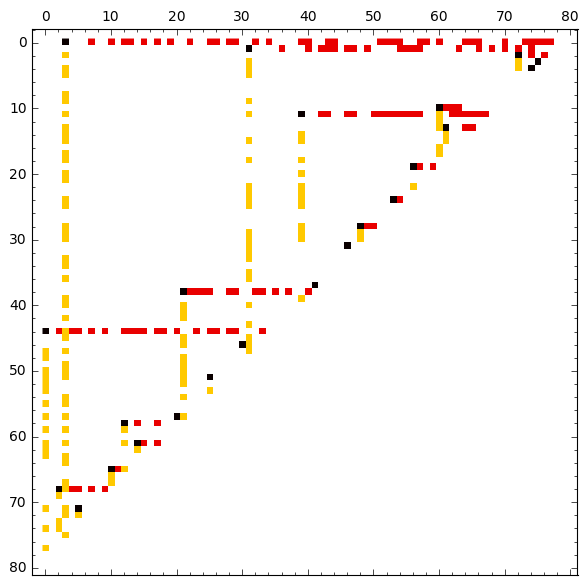
Figure 1: Support of the $\mathcal{L}$ (yellow), $\mathcal{E}$ (black) and $\mathcal{U}$ (red) matrices of the Bruhat generator for a $80\times 80$ left triangular matrix of quasiseparable order $5$.

As the supports of $\mathcal{L}$ and $\mathcal{U}$ are disjoint, the two matrices can be shown on the same left triangular matrix. The pivots of $\mathcal{E}$ (black) are the leading coefficients of every non-zero row of $\mathcal{U}$ and non-zero column of $\mathcal{L}$.

Corollary 4.16.

Any $(r_{L},r_{U})$-quasiseparable matrix of dimension $n\times n$ can be represented by a generator using no more than $2n(r_{L}+r_{U})+n-2(r_{L}^{2}-2r_{U}^{2})$ field elements.

4.3 The compact Bruhat generator

The sparse structure of the Bruhat generator makes it not amenable to the use of fast matrix arithmetic. We therefore propose here a slight variation of it, that we will use in section 5 for fast complexity estimates. We will first describe this compact representation for the $\mathcal{L}$ factor of the Bruhat generator.

First, remark that there exists a permutation matrix $\mathcal{Q}$ moving the non-zero columns of $\mathcal{L}$ to the first $r$ positions, sorted by increasing leading row index, i.e. such that $\mathcal{L}\mathcal{Q}$ is in column echelon form. The matrix $\mathcal{L}\mathcal{Q}$ is now compacted, but still has $r=\text{rank}(A)$ columns, which may exceed $s$ and thus preventing to reach complexities in terms of $n$ and $s$ only. We will again use the argument of Lemma 4.12 to produce a more compact representation with only $O(ns)$ non-zero elements, stored in dense blocks. Algorithm 3 shows how to build such a representation composed of a block diagonal matrix and a block sub-diagonal matrix, where all blocks have column dimension $s$: $\left[\begin{smallmatrix}\mathsf{D}_{1}\\ \mathsf{S}_{2}&\mathsf{D}_{2}\\ &\mathsf{S}_{3}&\mathsf{D}_{3}\\ &&\ddots&\ddots\\ &&&\mathsf{S}_{t}&\mathsf{D}_{t}\end{smallmatrix}\right].$

Algorithm 3 Compressing the Bruhat generator

1:$\mathcal{L}$: the first matrix of the Bruhat generator

2:$\mathsf{D},\mathsf{S},\mathsf{T},\mathcal{Q}$: the compression of $\mathcal{L}$

3:$\mathcal{Q}\leftarrow$ a permutation s.t. $\mathcal{L}\mathcal{Q}$ is in column echelon form

4:$\mathsf{C}\leftarrow\mathcal{L}\mathcal{Q}\left[\begin{smallmatrix}\mathsf{I}_{r}\\ \mathsf{0}\end{smallmatrix}\right]$ where $r=\text{rank}(\mathcal{L})$

5:Split $\mathsf{C}$ in column slices of width $s$.

6:$\triangleright$ $\mathsf{C}=\left[\begin{smallmatrix}\mathsf{C}_{11}&\\ \mathsf{C}_{21}&\mathsf{C}_{22}\\ \vdots&\vdots&\ddots\\ \mathsf{C}_{t1}&\mathsf{C}_{t2}&\dots&\mathsf{C}_{tt}\end{smallmatrix}\right]$ where $\mathsf{C}_{ii}$ is $k_{i}\times s$.

7:$\mathsf{D}\leftarrow\text{Diag}(\mathsf{C}_{11},\dots,\mathsf{C}_{tt})$

8: $\mathsf{C}\leftarrow\mathsf{C}-\mathsf{D}=\left[\begin{smallmatrix}\mathsf{0}\\ \mathsf{C}_{21}\\ \vdots&\ddots&\ddots\\ \mathsf{C}_{t1}&\dots&\mathsf{C}_{t,t-1}&\mathsf{0}\end{smallmatrix}\right]$

9:$\mathsf{T}\leftarrow\mathsf{I}_{n}$

10:for $i=3\dots t$ do

11:    for each non zero column $j$ of $\left[\begin{smallmatrix}\mathsf{C}_{i,i-2}\\ \dots\\ \mathsf{C}_{t,i-2}\end{smallmatrix}\right]$ do

12:          Let $k$ be a zero column of $\left[\begin{smallmatrix}\mathsf{C}_{i,i-1}\\ \dots\\ \mathsf{C}_{t,i-1}\end{smallmatrix}\right]$

13:          Move col. $j$ in $\left[\begin{smallmatrix}\mathsf{C}_{i,i-2}\\ \vdots\\ \mathsf{C}_{t,i-2}\end{smallmatrix}\right]$ to col. $k$ in $\left[\begin{smallmatrix}\mathsf{C}_{i,i-1}\\ \vdots\\ \mathsf{C}_{t,i-1}\end{smallmatrix}\right]$.

14:         $\mathsf{T}\leftarrow(\mathsf{I}_{n}+\mathsf{\Delta}^{(k,j)}-\mathsf{\Delta}^{(k,k)})\times\mathsf{T}$

15:    end for

16:end for

17:$\mathsf{S}\leftarrow\mathsf{C}=\left[\begin{smallmatrix}\mathsf{0}&\\ \mathsf{C}_{21}&\mathsf{0}\\ &\ddots&\ddots\\ &&\mathsf{C}_{t,t-1}&\mathsf{0}\end{smallmatrix}\right]$

18:Return $(\mathsf{D},\mathsf{S},\mathsf{T},\mathcal{Q})$

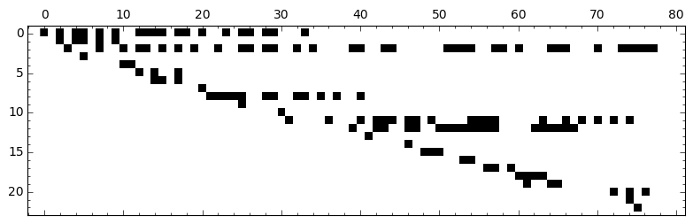
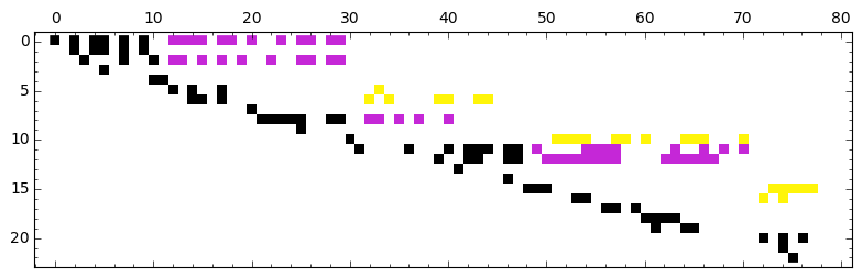
Figure 2: Support of the matrices $\mathcal{L}\mathcal{Q}$ (left), $\mathcal{P}\mathcal{U}$ (center) and of the corresponding compact Bruhat generator (right and bottom) for the matrix of Figure 1. In the compact Bruhat generator: $\mathsf{D}$ is in black and $\mathsf{S}$ in magenta and yellow; those rows and columns moved at step 13 of Algorithm 3 are in yellow.

Lemma 4.17.

Algorithm 3 computes a tuple $(\mathsf{D},\mathsf{S},\mathsf{T},\mathcal{Q})$ where $\mathcal{Q}$ is a permutation matrix putting $\mathcal{L}$ in column echelon form, $\mathsf{T}\in\{0,1\}^{r\times r}$, $\mathsf{D}=\text{Diag}(\mathsf{D}_{1},\dots,\mathsf{D}_{t})$, $\mathsf{S}=\left[\begin{smallmatrix}\mathsf{0}\\ \mathsf{S}_{2}&\mathsf{0}\\ &\ddots&\ddots\\ &&\mathsf{S}_{t}\end{smallmatrix}\right]$ where each $\mathsf{D}_{i}$ and $\mathsf{S}_{i}$ is $k_{i}\times s$ for $k_{i}\geq s$ and $\sum_{i=1}^{t}k_{i}=n$. This tuple is the compact Bruhat generator for $\mathcal{L}$ and satisfies $\mathcal{L}=\begin{bmatrix}\mathsf{D}+\mathsf{S}\mathsf{T}&\mathsf{0}_{n\times(n-r)}\end{bmatrix}\mathcal{Q}^{T}$.

Proof 4.18.

First, note that for every $i$, the dimensions of the blocks $\mathsf{S}_{i}$ and $\mathsf{D}_{i}$ are that of the block $\mathsf{C}_{ii}$. This block contains $s$ pivots, hence $k_{i}\geq s$. We then prove that there always exists a zero column to pick at step 12. The loci of the possible non-zero elements in $\mathcal{L}$ are column segments below a pivot and above the anti-diagonal. From Lemma 4.12, these segments have the property that each row of $\mathcal{L}$ is intersected by no more than $s$ of them. This property is preserved by column permutation, and still holds on the matrix $\mathsf{C}$. In the first row of $\begin{bmatrix}\mathsf{C}_{i1}&\dots&\mathsf{C}_{ii}\end{bmatrix}$, there is a pivot located in the block $\mathsf{C}_{ii}$. Hence there is at most $s-1$ such segments intersecting $\begin{bmatrix}\mathsf{C}_{i1}&\dots&\mathsf{C}_{i,i-1}\end{bmatrix}$. These $s-1$ columns can all be gathered in the block $\mathsf{C}_{i,i-1}$ of column dimension $s$.

There only remains to show that $\mathsf{S}\mathsf{T}$ is the matrix $\mathsf{C}$ of step 8. For every pair of indices $(j,k)$ selected in loop 10, right multiplication by $(\mathsf{I}_{n}+\mathsf{\Delta}^{(k,j)}-\mathsf{\Delta}^{(k,k)})$ adds up column $k$ to column $j$ and zeroes out column $k$. On matrix $\mathsf{S}$, this has the effect of reverting each operation done at step 13 in the reverse order of the loop 10.

A compact representation of $\mathcal{U}$ is obtained in Lemma 4.19 by running Algorithm 3 on $\mathcal{U}^{T}$ and transposing its output.

Lemma 4.19.

There exist a tuple $(\mathsf{D},\mathsf{S},\mathsf{T},\mathcal{P})$ called the compact Bruhat generator for $\mathcal{U}$ such that $\mathcal{P}$ is a permutation matrix putting $\mathcal{U}$ in row echelon form, $\mathsf{T}\in\{0,1\}^{r\times r}$, $\mathsf{D}=\text{Diag}(\mathsf{D}_{1},\dots,\mathsf{D}_{t})$, $\mathsf{S}=\left[\begin{smallmatrix}\mathsf{0}&\mathsf{S}_{2}\\ &\ddots&\ddots\\ &&\mathsf{0}&\mathsf{S}_{t}\end{smallmatrix}\right]$ where each $\mathsf{D}_{i}$ and $\mathsf{S}_{i}$ is $s\times k_{i}$ for $k_{i}\geq s$ and $\sum_{i=1}^{t}k_{i}=n$ and $\mathcal{U}=\mathcal{P}^{T}\begin{bmatrix}\mathsf{D}+\mathsf{T}\mathsf{S}\\ \mathsf{0}_{(n-r)\times n}\end{bmatrix}$.

According to (7), the reconstruction of the initial matrix $\mathsf{A}$, from the compact Bruhat generators, writes

$$\mathsf{A}=(\mathsf{D}_{\mathcal{L}}+\mathsf{S}_{\mathcal{L}}\mathsf{T}_{\mathcal{L}})\mathsf{R}(\mathsf{D}_{\mathcal{U}}+\mathsf{T}_{\mathcal{U}}\mathsf{S}_{\mathcal{U}})$$ (8)

where $\mathsf{R}$ is the leading $r\times r$ sub-matrix of $\mathcal{Q}^{T}\mathcal{E}^{T}\mathcal{P}^{T}$. As it has full rank, it is a permutation matrix.

This factorization is a compact version of the generalized Bruhat decomposition [13, 7]: the left factor is a column echelon form, the right factor a row echelon form.

5 Cost of computing with the new generators

5.1 Computation of the generators

5.1.1 The binary tree generators

Let $T_{1}(n,s)$ denote the cost of the computation of the binary tree generator for an $n\times n$ matrix of order of quasiseparability $s$. It satisfies the recurrence relation $T_{1}(n,s)=K_{\omega}s^{\omega-2}\left(\frac{n}{2}\right)^{2}+2T_{1}(n/2,s)$, which solves in

$$T(n,s)=\frac{K_{\omega}}{2}s^{\omega-2}n^{2}\text{ with }K_{\omega}=\frac{2^{\omega-2}}{(2^{\omega}-2)(2^{\omega-2}-1)}\mathsf{C}_{\omega}$$

where $C_{\omega}$ is the leading constant of the complexity of matrix multiplication [5].

5.1.2 The Bruhat generator

We propose in Algorithm 4 an evolution of Algorithm 2 to compute the factors of the Bruhat generator.

Algorithm 4 LT-Bruhat

1:$\mathsf{A}$: an $n\times n$ matrix

2:$(\mathcal{L},\mathcal{E},\mathcal{U})$: a Bruhat generator for the left triangular part of $\mathsf{A}$

3:if $n=1$ then return $([0],[0],[0])$

4:Split $\mathsf{A}=\begin{bmatrix}\mathsf{A_{1}}&\mathsf{A_{2}}\\ \mathsf{A_{3}}\end{bmatrix}$ where $\mathsf{A_{3}}$ is $\lfloor\frac{n}{2}\rfloor\times\lfloor\frac{n}{2}\rfloor$

5:Decompose $\mathsf{A_{1}}=\mathsf{P_{1}}\begin{bmatrix}\mathsf{L_{1}}\\ \mathsf{M_{1}}\end{bmatrix}\begin{bmatrix}\mathsf{U_{1}}&\mathsf{V_{1}}\end{bmatrix}\mathsf{Q_{1}}$ $\triangleright$ $\texttt{PLUQ}(\mathsf{A_{1}})$

6:$\mathsf{R_{1}}\leftarrow\mathsf{P_{1}}\begin{bmatrix}\mathsf{I_{r_{1}}}\\ &\mathsf{0}\end{bmatrix}\mathsf{Q_{1}}$ where $r_{1}=\text{rank}(\mathsf{A_{1}})$.

7:$\begin{bmatrix}\mathsf{B_{1}}\\ \mathsf{B_{2}}\end{bmatrix}\leftarrow\mathsf{P_{1}}^{T}\mathsf{A_{2}}$ $\triangleright$ $\texttt{PermR}(\mathsf{A_{2}},\mathsf{P_{1}}^{T})$

8:$\begin{bmatrix}\mathsf{C_{1}}&\mathsf{C_{2}}\end{bmatrix}\leftarrow\mathsf{A_{3}}\mathsf{Q_{1}}^{T}$ $\triangleright$ $\texttt{PermC}(\mathsf{A_{3}},\mathsf{Q_{1}}^{T})$

9:Here $A=\left[\begin{array}[]{cc|c}\mathsf{L_{1}}\backslash\mathsf{U_{1}}&\mathsf{V_{1}}&\mathsf{B_{1}}\\ \mathsf{M_{1}}&\mathsf{0}&\mathsf{B_{2}}\\ \hline\cr\mathsf{C_{1}}&\mathsf{C_{2}}&\\ \end{array}\right]$.

10:$\mathsf{D}\leftarrow\mathsf{L_{1}}^{-1}\mathsf{B_{1}}$ $\triangleright$ $\texttt{TRSM}(\mathsf{L_{1}},\mathsf{B_{1}})$

11:$\mathsf{E}\leftarrow\mathsf{C_{1}}\mathsf{U_{1}}^{-1}$ $\triangleright$ $\texttt{TRSM}(\mathsf{C_{1}},\mathsf{U_{1}})$

12:$\mathsf{F}\leftarrow\mathsf{B_{2}}-\mathsf{M_{1}}\mathsf{D}$ $\triangleright$ $\texttt{MM}(\mathsf{B_{2}},\mathsf{M_{1}},\mathsf{D})$

13:$\mathsf{G}\leftarrow\mathsf{C_{2}}-\mathsf{E}\mathsf{V_{1}}$ $\triangleright$ $\texttt{MM}(\mathsf{C_{2}},\mathsf{E},\mathsf{V_{1}})$

14:Here $\mathsf{A}=\left[\begin{array}[]{cc|c}\mathsf{L_{1}}\backslash\mathsf{U_{1}}&\mathsf{V_{1}}&\mathsf{D}\\ \mathsf{M_{1}}&\mathsf{0}&\mathsf{F}\\ \hline\cr\mathsf{E}&\mathsf{G}&\\ \end{array}\right]$.

15:$\mathsf{H}\leftarrow\mathsf{P_{1}}\begin{bmatrix}\mathsf{0}_{r_{1}\times\frac{n}{2}}\\ \mathsf{F}\end{bmatrix}$

16:$\mathsf{I}\leftarrow\begin{bmatrix}\mathsf{0}_{r_{1}\times\frac{n}{2}}&\mathsf{G}\end{bmatrix}\mathsf{Q_{1}}$

17: $(\mathcal{L}_{2},\mathcal{E}_{2},\mathcal{U}_{2})\leftarrow\texttt{LT-Bruhat}(\mathsf{H})$

18: $(\mathcal{L}_{3},\mathcal{E}_{3},\mathcal{U}_{3})\leftarrow\texttt{LT-Bruhat}(\mathsf{I})$

19:$\mathcal{L}\leftarrow\text{Left}\left(\begin{bmatrix}\mathsf{P}_{1}\\ &\mathsf{I}_{\frac{n}{2}}\end{bmatrix}\begin{bmatrix}\mathsf{L}_{1}\\ \mathsf{M}_{1}&\mathsf{0}\\ \mathsf{E}&\mathsf{0}\end{bmatrix}\begin{bmatrix}\mathsf{Q}_{1}\\ &\mathsf{I}_{\frac{n}{2}}\end{bmatrix}\right)+\begin{bmatrix}\mathsf{0}&\mathcal{L}_{2}\\ \mathcal{L}_{3}\end{bmatrix}$

20:$\mathcal{U}\leftarrow\begin{bmatrix}\mathsf{P}_{1}\begin{bmatrix}\mathsf{U}_{1}&V_{1}\\ \mathsf{0}&\mathsf{0}\end{bmatrix}\mathsf{Q}_{1}&\text{Left}(\mathsf{P}_{1}\begin{bmatrix}\mathsf{D}\\ \mathsf{0}\end{bmatrix})\\ \mathsf{0}&\mathsf{0}\end{bmatrix}+\begin{bmatrix}\mathsf{0}&\mathcal{U}_{2}\\ \mathcal{U}_{3}\end{bmatrix}$

21:$\mathcal{E}\leftarrow\begin{bmatrix}\mathcal{E}_{1}&\mathcal{E}_{2}\\ \mathcal{E}_{3}\end{bmatrix}$

22:return $(\mathcal{L},\mathcal{E},\mathcal{U})$

Theorem 5.20.

For any $n\times n$ matrix $\mathsf{A}$ with a left triangular part of quasiseparable order $s$, Algorithm 4 computes the Bruhat generator of the left triangular part of $\mathsf{A}$ in $O(s^{\omega-2}n^{2})$ field operations.

Proof 5.21.

The correctness of $\mathcal{E}$ is proven in Theorem 3.8. We will prove by induction the correctness of $\mathcal{U}$, noting that the correctness of $\mathcal{L}$ works similarly.

Let $\mathsf{H}=\mathsf{P}_{2}\mathsf{L}_{2}\mathsf{U}_{2}\mathsf{Q}_{2}$ and $\mathsf{I}=\mathsf{P}_{3}\mathsf{L}_{3}\mathsf{U}_{3}\mathsf{Q}_{3}$ be PLUQ decompositions of $\mathsf{H}$ and $\mathsf{I}$ revealing their rank profile matrices. Assume that Algorithm LT-Bruhat is correct in the two recursive calls 17 and 18, that is

$$\begin{array}[]{ll}\mathcal{U}_{2}=\text{Left}(\mathsf{P}_{2}\begin{bmatrix}\mathsf{U}_{2}\\ \mathsf{0}\end{bmatrix}\mathsf{Q}_{2}),&\mathcal{U}_{3}=\text{Left}(\mathsf{P}_{3}\begin{bmatrix}\mathsf{U}_{3}\\ \mathsf{0}\end{bmatrix}\mathsf{Q}_{3}),\\ \mathcal{L}_{2}=\text{Left}(\mathsf{P}_{2}\begin{bmatrix}\mathsf{L}_{2}&\mathsf{0}\end{bmatrix}\mathsf{Q}_{2}),&\mathcal{L}_{3}=\text{Left}(\mathsf{P}_{3}\begin{bmatrix}\mathsf{L}_{3}&\mathsf{0}\end{bmatrix}\mathsf{Q}_{3}).\\ \end{array}$$

At step 9, we have

$$\begin{bmatrix}\mathsf{A}_{1}&\mathsf{A}_{2}\\ \mathsf{A}_{3}&*\end{bmatrix} = \begin{bmatrix}\mathsf{P}_{1}\\ &\mathsf{I}_{\frac{n}{2}}\end{bmatrix}\left[\begin{array}[]{cc|c}\mathsf{L}_{1}&&\\ \mathsf{M}_{1}&\mathsf{I}_{\frac{n}{2}-r_{1}}\\ \hline\cr\mathsf{E}&\mathsf{0}&\mathsf{I}_{\frac{n}{2}}\end{array}\right]\times$$

$$\left[\begin{array}[]{cc|c}\mathsf{U}_{1}&\mathsf{V}_{1}&\mathsf{D}\\ &\mathsf{0}&\mathsf{F}\\ \hline\cr&\mathsf{G}&\end{array}\right]\begin{bmatrix}\mathsf{Q}_{1}\\ &\mathsf{I}_{\frac{n}{2}}\end{bmatrix}$$

As the first $r_{1}$ rows of $\mathsf{P}_{1}^{T}\mathsf{H}$ are zeros, there exists $\mathsf{\bar{P}}_{2}$ a permutation matrix and $\mathsf{\bar{L}}_{2}$, a lower triangular matrix, such that $\mathsf{P}_{1}^{T}\mathsf{P}_{2}\mathsf{L}_{2}=\begin{bmatrix}\mathsf{0}_{r_{1}\times\frac{n}{2}}\\ \mathsf{\bar{P}}_{2}\mathsf{\bar{L}}_{2}\end{bmatrix}$. Similarly, there exsist $\mathsf{\bar{Q}}_{3}$, a permutation matrix and $\mathsf{\bar{U}}_{3}$, an upper triangular matrix, such that $\mathsf{U}_{3}\mathsf{Q}_{3}\mathsf{Q}_{1}^{T}=\begin{bmatrix}\mathsf{0}_{\frac{n}{2}\times r_{1}}&\mathsf{\bar{U}}_{3}\mathsf{\bar{Q}}_{3}\end{bmatrix}$. Hence

$$\begin{bmatrix}\mathsf{A}_{1}&\mathsf{A}_{2}\\ \mathsf{A}_{3}&*\end{bmatrix} = \begin{bmatrix}\mathsf{P}_{1}\\ &\mathsf{P}_{3}\end{bmatrix}\left[\begin{array}[]{cc|c}\mathsf{L}_{1}&&\\ \mathsf{M}_{1}&\mathsf{\bar{P}}_{2}\mathsf{\bar{L}}_{2}\\ \hline\cr\mathsf{P}_{3}^{T}\mathsf{E}&\mathsf{0}&\mathsf{L}_{3}\end{array}\right]\times$$

$$\left[\begin{array}[]{cc|c}\mathsf{U}_{1}&\mathsf{V}_{1}&\mathsf{D}\mathsf{Q}_{2}^{T}\\ &\mathsf{0}&\mathsf{U_{2}}\\ &\mathsf{\bar{U}}_{3}\mathsf{\bar{Q}}_{3}\end{array}\right]\begin{bmatrix}\mathsf{Q}_{1}\\ &\mathsf{Q}_{2}\end{bmatrix}$$

Setting $\mathsf{N}_{1}=\mathsf{\bar{P}}_{2}^{T}\mathsf{M}_{1}$ and $\mathsf{W}_{1}=\mathsf{V}_{1}\mathsf{\bar{Q}}_{3}^{T}$, we have

$$\begin{bmatrix}\mathsf{A}_{1}&\mathsf{A}_{2}\\ \mathsf{A}_{3}&*\end{bmatrix} = \begin{bmatrix}\mathsf{P}_{1}\begin{bmatrix}\mathsf{I}_{r_{1}}\\ &\mathsf{\bar{P}}_{2}\end{bmatrix}\\ &\mathsf{P}_{3}\end{bmatrix}\left[\begin{array}[]{ccc}\mathsf{L}_{1}\\ \mathsf{N}_{1}&\mathsf{\bar{L}}_{2}\\ \hline\cr\mathsf{E}&\mathsf{0}&\mathsf{\mathsf{L_{3}}}\end{array}\right]\times$$

$$\left[\begin{array}[]{cc|c}\mathsf{U}_{1}&\mathsf{W}_{1}&\mathsf{D}\mathsf{Q}_{2}^{T}\\ &\mathsf{0}&\mathsf{U_{2}}\\ &\mathsf{\bar{U}}_{3}\end{array}\right]\begin{bmatrix}\begin{bmatrix}\mathsf{I}_{r_{1}}\\ &\mathsf{\bar{Q}}_{3}\end{bmatrix}\mathsf{Q}_{1}\\ &\mathsf{Q}_{2}\end{bmatrix}.$$

A PLUQ of $\left[\begin{smallmatrix}\mathsf{A}_{1}&\mathsf{A}_{2}\\ \mathsf{A}_{3}\end{smallmatrix}\right]$ revealing its rank profile matrix is then obtained from this decomposition by a row block cylic-shift on the second factor and a column block cyclic shift on the third factor as in [5, Algorithm 1].

Finally,

$$\begin{split}\mathsf{P}\begin{bmatrix}\mathsf{U}\\ 0\end{bmatrix}\mathsf{Q}=\begin{bmatrix}\mathsf{P}_{1}\\ &\mathsf{I}_{\frac{n}{2}}\end{bmatrix}\begin{bmatrix}\mathsf{U}_{1}&\mathsf{V}_{1}&\mathsf{D}\\ &\mathsf{0}&\mathsf{\bar{P}}_{2}\mathsf{U}_{2}\mathsf{Q}_{2}\\ &\mathsf{P}_{3}\mathsf{\bar{U}}_{3}\mathsf{\bar{Q}}_{3}\\ \mathsf{0}&\mathsf{0}&\mathsf{0}\end{bmatrix}\begin{bmatrix}\mathsf{Q}_{1}\\ &\mathsf{I}_{\frac{n}{2}}\end{bmatrix}\\ =\begin{bmatrix}\mathsf{P}_{1}\begin{bmatrix}\mathsf{U}_{1}&\mathsf{V}_{1}\\ \mathsf{0}&\mathsf{0}\end{bmatrix}\mathsf{Q}_{1}&\mathsf{P}_{1}\begin{bmatrix}\mathsf{D}\\ \mathsf{0}\end{bmatrix}\\ \mathsf{0}&\mathsf{0}\ \end{bmatrix}+\begin{bmatrix}&\mathsf{P}_{2}\begin{bmatrix}\mathsf{U}_{2}\\ \mathsf{0}\end{bmatrix}\mathsf{Q}_{2}\\ \mathsf{P}_{3}\begin{bmatrix}\mathsf{U}_{3}\\ \mathsf{0}\end{bmatrix}\mathsf{Q}_{3}\end{bmatrix}.\end{split}$$

Hence

$$\text{Left}(\mathsf{P}\mathsf{U}\mathsf{Q})=\begin{bmatrix}\mathsf{P}_{1}\begin{bmatrix}\mathsf{U}_{1}&\mathsf{V}_{1}\\ \mathsf{0}&\mathsf{0}\end{bmatrix}\mathsf{Q}_{1}&\text{Left}(\mathsf{P}_{1}\begin{bmatrix}\mathsf{D}\\ \mathsf{0}\end{bmatrix})\\ \mathsf{0}&\mathsf{0}\\ \end{bmatrix}+\begin{bmatrix}&\mathcal{U}_{2}\\ \mathcal{U}_{3}\end{bmatrix}.$$

The complexity analysis is exactly that of Theorem 3.8.

The computation of a compact Bruhat generator is obtained by combining Algorithm 4 with Algorithm 3.

5.2 Applying a vector

For the three generators proposed earlier, the application of a vector to the corresponding left triangular matrix takes the same amount of field operations as the number of coefficients used for its representation. This yields a cost of $O(n(r_{L}\log\frac{n}{r_{L}}+r_{U}\log\frac{n}{r_{U}}))$ field operations for multiplying a vector to an $(r_{L},r_{U})$-quasiseparable matrix using the binary tree PLUQ generator and $O(n(r_{L}+r_{U}))$ using either one of the Bruhat generator or its compact variant.

5.3 Multiplying two left-triangular matrices

5.3.1 The binary tree PLUQ generator

Let $T_{\text{RL}}(n,s)$ denote the cost of multiplying a dense $s\times n$ matrix by a left triangular quasiseparable matrix of order $s$. The natural divide and conquer algorithm yields the recurrence formula:

$$T_{\text{RL}}(n,s)=2T_{\text{RL}}(n/2,s)+O(ns^{\omega-1})=O(ns^{\omega-1}\log{\frac{n}{s}}).$$

Let $T_{\text{PL}}(n,s)$ denote the cost of multiplying a PLUQ decomposition of dimension n and rank $s\leq n/2$ with a left triangular quasiseparable matrix of order $s$. The product can be done in

$$T_{\text{PL}}(n,s) = T_{\text{RL}}(n,s)+O(n^{2}s^{\omega-2})=O(n^{2}s^{\omega-2}).$$

Lastly, let $T_{\text{LL}}(n,s)$ denote the cost of multiplying two left-triangular matrices of quasiseparability order $s$. Again the natural recursive algorithm yields:

$$T_{\text{LL}}(n,s) = 2T_{\text{LL}}(n/2,s)+2T_{\text{PL}}(n/2,s)+O(n^{2}s^{\omega-2})$$

$$= O(n^{2}s^{\omega-2})$$

5.3.2 The Bruhat generator

Using the decomposition (8), the product of two left triangular matrices writes $\mathsf{A}\times\mathsf{B}=\mathsf{C}_{\mathsf{A}}\mathsf{R}_{\mathsf{A}}\mathsf{E}_{\mathsf{A}}\times\mathsf{C}_{\mathsf{B}}\mathsf{R}_{\mathsf{B}}\mathsf{E}_{\mathsf{B}}$ where $\mathsf{C}_{\mathsf{X}}=\mathsf{D}_{\mathcal{L}_{\mathsf{X}}}+\mathsf{S}_{\mathcal{L}_{\mathsf{X}}}\mathsf{T}_{\mathcal{L}_{\mathsf{X}}}$ and $\mathsf{E}_{\mathsf{X}}=\mathsf{D}_{\mathcal{U}_{\mathsf{X}}}+\mathsf{T}_{\mathcal{U}_{\mathsf{X}}}\mathsf{S}_{\mathcal{U}_{\mathsf{X}}}$ for $\mathsf{X}\in\{\mathsf{A},\mathsf{B}\}$. We will compute it using the following parenthesizing:

$$\mathsf{A}\times\mathsf{B}=\mathsf{C}_{\mathsf{A}}(\mathsf{R}_{\mathsf{A}}(\mathsf{E}_{\mathsf{A}}\times\mathsf{C}_{\mathsf{B}})\mathsf{R}_{\mathsf{B}})\mathsf{E}_{\mathsf{B}}.$$ (15)

The product $\mathsf{E}_{\mathsf{A}}\times\mathsf{C}_{\mathsf{B}}=(\mathsf{D}_{\mathcal{U}_{\mathsf{A}}}+\mathsf{T}_{\mathcal{U}_{\mathsf{A}}}\mathsf{S}_{\mathcal{U}_{\mathsf{A}}})(\mathsf{D}_{\mathcal{L}_{\mathsf{B}}}+\mathsf{S}_{\mathcal{L}_{\mathsf{B}}}\mathsf{T}_{\mathcal{L}_{\mathsf{B}}})$ only consists in multiplying together block diagonal or sub-diagonal matrices $n\times r_{B}$ or $r_{A}\times n$. We will describe the product of two block diagonal matrices (flat times tall); the other cases with sub-diagonal matrices work similarly.

Each term to be multiplied is decomposed in a grid of $s\times s$ tiles (except at the last row and column positions). In this grid, the non-zero blocks are non longer in a block-diagonal layout: in a flat matrix, the leading block of a block row may lie at the same block column position as the trailing block of its preceding block row, as shown in Figure 3.

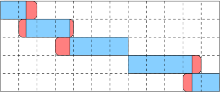
Figure 3: Aligning a block diagonal matrix (blue) on an $s\times s$ grid. Each block row of the aligned structure (red) may overlap with the previous and next block rows on at most one $s\times s$ tile on each side.

However, since $k_{i}\geq s$ for all $i$, no more than two consecutive block rows of a flat matrix lie in the same block column. Consequently these terms can be decomposed as a sum of two block diagonal matrices aligned on an $s\times s$ grid. Multiplying two such matrices costs $O(s^{\omega-1}n)$ which is consequently also the cost of computing the product $\mathsf{E}_{\mathsf{A}}\mathsf{C}_{\mathsf{B}}$. After left and right multiplication by the permutations $\mathsf{R}_{\mathsf{A}}$ and $\mathsf{R}_{\mathsf{B}}$, this $r_{\mathsf{A}}\times r_{\mathsf{B}}$ dense matrix is multiplied to the left by $\mathsf{C}_{\mathsf{A}}$. This costs $O(nr_{B}s^{\omega-2})$. Lastly, the right multiplication by $\mathsf{E}_{B}$ of the resulting $n\times r_{\mathsf{A}}$ matrix costs $O(n^{2}s^{\omega-2})$ which dominates the overall cost.

5.4 Multiplying two quasiseparable matrices

Decomposing each multiplicand into its upper, lower and diagonal terms, a product of two quasiseparable matrices writes $\mathsf{A}\times\mathsf{B}=(\mathsf{L}_{\mathsf{A}}+\mathsf{D}_{\mathsf{A}}+\mathsf{U}_{\mathsf{A}})(\mathsf{L}_{\mathsf{B}}+\mathsf{D}_{\mathsf{B}}+\mathsf{U}_{\mathsf{B}}).$ Beside the scaling by diagonal matrices, all other operations involve a product between any combination of lower an upper triangular matrices, which in turn translates into products of left triangular matrices and $\mathsf{J}_{n}$ as shows in Table 1.

$\times$	Lower	Upper
Lower	$\mathsf{J}_{n}\times\text{Left}\times\mathsf{J}_{n}\times\text{Left}$	$\mathsf{J}_{n}\times\text{Left}\times\text{Left}\times\mathsf{J}_{n}$
Upper	$\text{Left}\times\mathsf{J}_{n}\times\mathsf{J}_{n}\times\text{Left}$	$\text{Left}\times\mathsf{J}_{n}\times\text{Left}\times\mathsf{J}_{n}$

Table 1: Reducing products of lower and upper to products of left triangular matrices.

The complexity of section 5.3 directly applies for the computation of $\text{Upper}\times\text{Lower}$ and $\text{Lower}\times\text{Upper}$ products. For the other products, a $\mathsf{J}_{n}$ factor has to be added between the $\mathsf{E}_{\mathsf{A}}$ and $\mathsf{C}_{\mathsf{B}}$ factors in the innermost product of (15). As reverting the row order of $\mathsf{C}_{\mathsf{B}}$ does not impact the cost of computing this product, the same complexity applies here too.

Theorem 5.22.

Mutliplying two quasiseparable matrices of order respectively $(l_{\mathsf{A}},u_{\mathsf{A}})$ and $(l_{\mathsf{B}},u_{\mathsf{B}})$ costs $O(n^{2}s^{\omega-2})$ field operations where $s=\max(l_{\mathsf{A}},u_{\mathsf{A}},l_{\mathsf{B}},u_{\mathsf{B}})$, using either one of the binary tree or the compact Bruhat generator.

6 Perspectives

The algorithms proposed for multiplying two quasiseparable matrices output a dense $n\times n$ matrix in time $O(n^{2}s^{\omega-2})$ for $s=\max(l_{\mathsf{A}},u_{\mathsf{A}},l_{\mathsf{B}},u_{\mathsf{B}})$. However, the product is also a quasiseparable matrix, of order $({l_{\mathsf{A}}}+{l_{\mathsf{B}}},{u_{\mathsf{A}}}+{u_{\mathsf{B}}})$ [8, Theorem 4.1], which can be represented by a Bruhat generator with only $O(n({l_{\mathsf{A}}}+{l_{\mathsf{B}}}+{u_{\mathsf{A}}}+{u_{\mathsf{B}}}))$ coefficients. A first natural question is thus to find an algorithm computing this representation from the generators of $\mathsf{A}$ and $\mathsf{B}$ in time $O(ns^{\omega-1})$.

Second, a probabilistic algorithm [7, § 7] reduces the complexity of computing the rank profile matrix to $O\tilde{\ }(n^{2}+r^{\omega})$. It is not clear whether it can be applied to compute a compact Bruhat generator in time $O\tilde{\ }(n^{2}+\max(l_{\mathsf{A}},u_{\mathsf{A}})^{\omega})$.

Note (added Sept. 16, 2016.)

Equation (15) for the multiplication of two Bruhat generators is missing the Left operators, and is therefore incorrect. The target complexities can still be obtained by slight modification of the algorithm: computing the inner-most product $\mathsf{E}_{\mathsf{A}}\times\mathsf{C}_{\mathsf{B}}$ as an unevaluated sum of blocks products. This will be detailed in a follow-up paper.

References

- [1] P. Boito, Y. Eidelman, and L. Gemignani. Implicit QR for companion-like pencils. Math. of Computation, 85(300):1753–1774, 2016.
- [2] Tony F. Chan. Rank revealing QR factorizations. Linear Algebra and its Applications, 88:67–82, April 1987.
- [3] S. Chandrasekaran and I. Ipsen. On Rank-Revealing Factorisations. SIAM Journal on Matrix Analysis and Applications, 15(2):592–622, April 1994.
- [4] S. Delvaux and M. Van Barel. A Givens-Weight Representation for Rank Structured Matrices. SIAM J. on Matrix Analysis and Applications, 29(4):1147–1170, November 2007.
- [5] Jean-Guillaume Dumas, Clément Pernet, and Ziad Sultan. Simultaneous computation of the row and column rank profiles. In Manuel Kauers, editor, Proc. ISSAC’13, pages 181–188. ACM Press, 2013.
- [6] Jean-Guillaume Dumas, Clément Pernet, and Ziad Sultan. Computing the rank profile matrix. In Proc. ISSAC’15, pages 149–156, New York, NY, USA, 2015. ACM.
- [7] Jean-Guillaume Dumas, Clément Pernet, and Ziad Sultan. Fast computation of the rank profile matrix and the generalized bruhat decomposition. Technical report, 2015. arXiv:1601.01798.
- [8] Y. Eidelman and I. Gohberg. On a new class of structured matrices. Integral Equations and Operator Theory, 34(3):293–324, September 1999.
- [9] Yuli Eidelman, Israel Gohberg, and Vadim Olshevsky. The QR iteration method for hermitian quasiseparable matrices of an arbitrary order. Linear Algebra and its Applications, 404:305 – 324, 2005.
- [10] Tsung-Min Hwang, Wen-Wei Lin, and Eugene K. Yang. Rank revealing LU factorizations. Linear Algebra and its Applications, 175:115–141, October 1992.
- [11] K Lessel, M. Hartman, and Shivkumar Chandrasekaran. A fast memory efficient construction algorithm for hierarchically semi-separable representations. Technical report, 2015. http://scg.ece.ucsb.edu/publications/MemoryEfficientHSS.pdf.
- [12] Gennadi Ivanovich Malaschonok. Fast generalized Bruhat decomposition. In CASC’10, volume 6244 of LNCS, pages 194–202. Springer-Verlag, Berlin, Heidelberg, 2010.
- [13] Wilfried Manthey and Uwe Helmke. Bruhat canonical form for linear systems. Linear Algebra and its Applications, 425(2–3):261 – 282, 2007. Special Issue in honor of Paul Fuhrmann.
- [14] C.-T. Pan. On the existence and computation of rank-revealing LU factorizations. Linear Algebra and its Applications, 316(1–3):199–222, September 2000.
- [15] The LinBox Group. LinBox: Linear algebra over black-box matrices, v1.4.1 edition, 2016. http://linalg.org/.
- [16] R. Vandebril, M. Van Barel, G. Golub, and N. Mastronardi. A bibliography on semiseparable matrices. CALCOLO, 42(3):249–270, 2005.
- [17] Raf Vandebril, Marc Van Barel, and Nicola Mastronardi. Matrix computations and semiseparable matrices: linear systems, volume 1. The Johns Hopkins University Press, 2007.
- [18] Jianlin Xia, Shivkumar Chandrasekaran, Ming Gu, and Xiaoye S. Li. Fast algorithms for hierarchically semiseparable matrices. Numerical Linear Algebra with Applications, 17(6):953–976, December 2010.