Using separable non-negative matrix factorization techniques for the analysis of time-resolved Raman spectra

Abstract

The key challenge of time-resolved Raman spectroscopy is the identification of the constituent species and the analysis of the kinetics of the underlying reaction network. In this work we present an integral approach that allows for determining both the component spectra and the rate constants simultaneously from a series of vibrational spectra. It is based on an algorithm for non-negative matrix factorization which is applied to the experimental data set following a few pre-processing steps. As a prerequisite for physically unambiguous solutions, each component spectrum must include one vibrational band that does not significantly interfere with vibrational bands of other species. The approach is applied to synthetic “experimental” spectra derived from model systems comprising a set of species with component spectra differing with respect to their degree of spectral interferences and signal-to-noise ratios. In each case, the species involved are connected via monomolecular reaction pathways. The potential and limitations of the approach for recovering the respective rate constants and component spectra are discussed.

1 Introduction

Raman spectroscopy is a versatile tool to probe molecular structure changes that are associated with the temporal evolution of chemical or physical processes [21, 3, 20]. Since time-resolved Raman spectroscopy is applicable in a wide dynamic range down to the femtosecond time scale, it is capable to monitor quite different events, including intramolecular rearrangements in the excited state as well as chemical reactions in the ground state. The individual Raman spectra measured as a function of time represent a superposition of the intrinsic spectra of the individual species or molecular states that are involved in the reaction sequence. The relative contributions of the various spectra to each measured spectrum then reflect the actual composition of the sample at the respective time, and hence the entire series of experimental spectra represents the kinetics of the underlying processes. While just this information can also be provided by other transient optical techniques, the unique advantage of time-resolved Raman spectroscopy resides in the fact that the molecular structure of the individual species is encoded in the respective component spectra. This allows for identifying intermediate states and characterizing their structural and electronic properties as a prerequisite for determining the molecular reaction mechanism. The central task is, therefore, to disentangle the series of time-resolved Raman spectra in terms of the individual component spectra and their temporal evolution.

In the past decades, different concepts were designed for analyzing sets of complex Raman spectra [8, 14, 15, 22]. In most cases, these efforts were spurred by the concomitant vivid development in Raman and IR spectroscopic investigation of cellular systems for biological and medical applications.[23, 4] These studies are dedicated to classify and to distinguish microorganisms or to identify pathological tissues. To achieve these objectives, it is necessary to determine spectral signatures of a complex ensemble of biomolecules in a certain environment that are characteristic of a specific type or state of the cellular system. In these cases, analytical methods for pattern recognition are required which, in view of the large number of experimental spectra, are based on statistical procedures, such as principal component analysis, factor analysis, or singular value decomposition[8, 14, 15, 22, 23, 4, 27, 28]. Such approaches provide mathematical solutions but typically not the intrinsic spectra of the large number of pure components. Thus, extending multivariate analyses to a series of spectra reflecting physical or chemical changes of well-defined molecular species may just afford the number of the species involved but not necessarily their component spectra.

Such systems, on the other hand, are frequently treated by least-square methods in which either single Lorentzian/Gaussian bands and complete component spectra (component analysis) are employed to achieve a global fit to all experimental spectra[8]. The component analysis is quite robust as the number of degrees of freedom in the fitting process just corresponds to the number of components, given that all component spectra are known a priori. If, however, this is not the case, the “intuition” factor gains weight and thus the overall error increases substantially with the number of unknown component spectra.

In this work, we tried to overcome these drawbacks by developing an unsupervised analytical method that is based on non-negative matrix factorization (NMF). Such NMF techniques have rarely been used for factor analysis, with two notable exceptions[1, 19]. Unlike these previous approaches, our method takes advantage of the so-called separability inherent to the measurement data.

This paper is organized as follows. In Section 2 we present the mathematical model and describe the so-called separability condition that is derived from the specific properties of complex Raman spectra composed by a finite number of component spectra. Section 3 then describes the numerical method for computing the NMF and extracting the reaction coefficients. In Section 4 we illustrate on a sequence of artificial first-order reactions the reliability of our method under interference among the component spectra and under measurement noise. Concluding remarks are given in Section 5.

2 Mathematical background

2.1 Model for time-resolved Raman spectra of chemical reactions

Mathematically, the acquired measurements correspond to certain convex combinations of sums of Lorentz functions or Lorentzians that constitute the Raman spectra of the individual reactants. We will formalize our notion of the model in this section.

A Lorentzian $L_{x_{0},\gamma,I}(x)$ is a non-negative “peak function” with its maximum at the base point $x_{0}\in\mathbb{R}$ (corresponding to the frequency of the normal mode), the width at half-height $\gamma>0$ and the intensity $I>0$, which is defined by

$$L_{x_{0},\gamma,I}(x)=I\tfrac{\gamma^{2}}{(x-x_{0})^{2}+\gamma^{2}}.$$ (1)

For simplicity we will usually skip the parameters $x_{0},\gamma,I$ and simply write $L(x)$.

Consider a chemical reaction with $r$ reactant species. Then the Raman spectrum $w_{s}$ of each reactant can be modeled as a non-negative sum of $q_{s}$ Lorentzians, so that

$$w_{s}(x)=\sum_{k=1}^{q_{s}}L^{s}_{k}(x),\quad s=1,\dots,r.$$ (2)

We assume that all base points (or “peaks”) are located in the finite interval $[f_{l},f_{u}]\subset\mathbb{R}_{+}\mathrel{\mathop{:}}=[0,\infty)$. Note that one could also implement a model where the individual spectra are given by sums of Lorentzians and Gaussians, or Gaussians only.

Now we will consider the relative concentrations of the reactant species. We denote the concentration function of species $s$ by

$$h_{s}:[0,T]\rightarrow[0,1],\quad s=1,\dots,r,$$

so that $h_{s}(t)$ corresponds to the relative concentration of species $s$ at time $t\in[0,T]$ of the reaction. Consequently, at each time $t$ the $r$ concentrations sum to $1.0$. The functions $h_{s}(t)$ represent the reaction kinetics.

In this functional setting, the time-resolved vibrational Raman spectrum of the reaction can be modeled as

$$M(x,t)=\sum_{s=1}^{r}w_{s}(x)h_{s}(t)=\sum_{s=1}^{r}\left(\sum_{k=1}^{q_{s}}L^{s}_{k}(x)\right)h_{s}(t).$$ (3)

Discretizing (3) over time through $0=t_{0}<\cdots<t_{n-1}=T$ in $n$ time steps, and over frequencies through $f_{l}=x_{1}<\cdots<x_{m}=f_{u}$ in $m$ frequencies, models the measured data from the reaction. We denote the resulting measurement matrix by $M=[m_{ij}]=[M(x_{i},t_{j+1})]\in\mathbb{R}_{+}^{m,n}$.

Now we discretize the functions $w_{s}(x)$ over the frequencies and obtain the vectors

$$w_{s}=[w_{s}(x_{1}),\dots,w_{s}(x_{m})]^{T}\in\mathbb{R}_{+}^{m},\quad s=1,\dots,r,$$

as well as the matrix $W=[w_{1},\dots,w_{r}]\in\mathbb{R}_{+}^{m,r}$. Similarly, we discretize the functions $h_{s}(t)$ over time and obtain the vectors

$$h_{s}=[h_{s}(t_{0}),\dots,h_{s}(t_{n-1})]^{T}\in\mathbb{R}_{+}^{n},\quad s=1,\dots,r,$$

as well as the matrix

$$H=\begin{bmatrix}h_{1}^{T}\\ \vdots\\ h_{r}^{T}\end{bmatrix}\in\mathbb{R}_{+}^{r,n}.$$

Then the measurement matrix $M$, which includes all experimental spectra, can be written as

$$M=\sum_{s=1}^{r}w_{s}h_{s}^{T}=WH,$$ (4)

i.e., the entry-wise non-negative matrix $M$ is the product of the two entry-wise non-negative matrices $W$ and $H$.

2.2 NMF for Raman experimental data

The task of analyzing time-resolved Raman spectroscopic data consists of (1) determining the spectra of the individual species (component spectra), and (2) identifying the underlying reaction kinetics. Using the notation from Section 2.1, the corresponding mathematical problem is as follows: Given the non-negative data matrix $M\in\mathbb{R}_{+}^{m,n}$, and assuming that the reaction involves $r$ species, find non-negative matrices $W\in\mathbb{R}_{+}^{m,r}$ and $H\in\mathbb{R}_{+}^{r,n}$ such that

$$M=WH.$$ (5)

Note that a factorization of the form (5) where $W$ and/or $H$ have negative entries has no physical meaning, as neither a measured intensity nor a relative concentration can be negative.

The mathematical task of finding a non-negative matrix factorization (NMF) of $M$ is one of formidable difficulty: Without further assumptions on the given data, the problem is ill-posed and its solutions are non-unique in general. From a complexity point of view, NMF is NP-hard[26]. Moreover, an exact factorization as in (5) is more a theoretical desire than achievable in practice. The presence of noise or other forms of data uncertainty may simply rule out the existence of such a factorization.

The theory and computation of non-negative matrix factorizations is a very active research topic, whose popularity gained much from an article by Lee and Seung on the use of NMF for feature extraction[17]; an earlier work on NMF dates back to 1974[24]. A useful overview is given in the recent survey by Gillis[11].

A practically much better justified view is adopted by considering NMF as an approximation problem rather than an exact factorization. The usual way to give a formal definition of this approximation problem is as follows: Let $\lVert\cdot\lVert$ be a matrix norm. Given the non-negative data matrix $M$, we seek non-negative matrices $W$ and $H$ such that

$$\lVert M-WH\lVert$$

is small. The norm plays the role of a “distance function” and measures how close the eventually found factors $W$, $H$ reproduce the given data. In this work we mostly use the Frobenius norm, which for any (rectangular) matrix $A=[a_{ij}]$ is defined by $\|A\|_{F}=\sqrt{\sum_{i,j}|a_{ij}|^{2}}$.

When treating time-resolved Raman data on chemical reactions, another problem of interest arises. Usually one does not know the number of intermediate species in the reaction. Thus the required information to set up an NMF problem, $r$, is missing. To overcome this shortcoming, one may assume that $r$ is not very large (in practice it is often between two and ten). It then is a simple matter of trying different values for $r$ and selecting the best solution (see Section 4.5). Another heuristic estimate is available by the number of “large” singular values of the matrix $M$[18].

2.3 The separability condition

While the general NMF problem introduced in Section 2.2 is very difficult in general, there is a very important special case, the so-called separable NMF problem [7, 2]. As before, the measurement matrix is denoted by $M\in\mathbb{R}_{+}^{m,n}$, and the entries of each row of $M$ sum to $1.0$. (This can always be achieved by applying a diagonal scaling matrix from the left.) Algebraically, the data matrix $M$ is called $r$-separable, if it can be written in the form

$$M=WH=Q\begin{bmatrix}I_{r}\\ W^{\prime}\end{bmatrix}H,$$ (6)

where $I_{r}$ is the $r$-by-$r$ identity matrix, and $Q\in\mathbb{R}^{m,m}$ is a permutation matrix. Separability implies that all the rows of $M$ can be reconstructed by using only $r$ rows of $M$ (these constitute the factor $H$) by convex combinations with weights given through $W^{\prime}$.

The separability condition in equation (6) can be interpreted in the model for time-resolved Raman spectroscopy data from the previous section as follows. The measurement matrix $M$ is separable when each species $s$, represented by the $s$-th column of $W$, has a characteristic frequency $x_{s}$ at which $w_{s}(x_{s})>0$ (see (2)), but $w_{\tilde{s}}(x_{s})=0$ for all other species $\tilde{s}\neq s$. If such a frequency is present for each species, the measurement matrix $M$ contains rows that are equal to the rows of the sought-for kinetic matrix $H$. Thus, the primary task is to determine the characteristic frequencies. For example, if all the species involved in the reaction contain a Lorentz band that does not interfere with a Lorentz band of any other species, then the separability condition is satisfied.

However, recall from the definition (1) that the intensity of a Lorentzian $L_{x_{0},\gamma,I}(x)$ vanishes reciprocally to a quadratic function in the distance from the base frequency $x_{0}$. In particular, the separability condition as explained above cannot be satisfied in any case, since $w_{s}(x)>0$ for every species $s$ and frequency $x$. Consequently, the factorization (4) will not exactly be separable (in the theoretical framework of Section 2.1).

While an exact interference-free set of characteristic frequencies is in general impossible, the interference can be numerically small or even zero if the corresponding base frequencies of the characteristic bands are sufficiently far apart. Algebraically, it means that instead of the exact separability condition (6), our problem is properly described by a near-separable problem, meaning that

$$M=WH=Q\begin{bmatrix}I_{r}+R\\ W^{\prime}\end{bmatrix}H=Q\begin{bmatrix}I_{r}\\ W^{\prime}\end{bmatrix}H+\underbrace{Q\begin{bmatrix}R\\ 0\end{bmatrix}H}_{=\mathrel{\mathop{:}}N_{I}}=Q\begin{bmatrix}I_{r}\\ W^{\prime}\end{bmatrix}H+N_{I}.$$ (7)

Here we interpret the matrix $N_{I}$ as noise originating from interference of the species at frequencies at which some species is strongly dominant in comparison with the other species. If $\|N_{I}\|$ is small, the original factors $W,H$ may be well approximated by applying an algorithm for separable NMF to $M$. Quantitative investigations on the allowable noise for some algorithms have been persued in a purely mathematical context.[13, 9, 12]

In Section 4.3, we provide a numerical study on a model problem that shows the effect of growing $\lVert N_{I}\lVert$ on the overall approximation quality.

So far we considered only ideal, noise free data measurements. Real experimental data involve measurement noise, and hence

$$M=WH+N_{M},$$ (8)

where we assume the noise to be purely additive, i.e. $N_{M}$ is componentwise non-negative. Algebraically, the measurement noise is no different from the noise arising from interference. The effect of measurement noise is studied numerically in Section 4.4.

Note that the separability assumption is widely used in other fields, such as hyperspectral imaging, text mining, or other blind source separation applications [16, 5, 6]. In some of these contexts, the separability assumption is assumed to be satisfied with respect to the time axis (in our notation, for $M^{T}$). In our application this would mean that for each species there exists some point in time at which the relative concentration of the species is $1.0$, which is highly unlikely for a typical reaction.

3 Computational method

The method we use for the identification of the reaction kinetics is based on the successive non-negative projection algorithm (SNPA) [10]. SNPA is an algorithm for computing the factor $H$ in (6) (the kinetics), provided that the problem at hand is near-separable. In the language of Section 2.3, we use SNPA to compute approximate characteristic frequencies of the species. We have chosen SNPA for its computational speed and robustness with respect to noise, but any other algorithm for separable NMF could be used as well.

While SNPA is at the center of our method, we also need to deal with a number of other computational tasks. The overall method is shown in Algorithm 1.

Algorithm 1 Species and kinetics identification via separable NMF

0:  Data matrix $M$, number of species $r$

0:  Approximate species $W$ and kinetics $H$ s.t. $M\approx WH$; reaction coefficients $K$.

1:  Filter out noisy rows (frequencies) of $M$.

2:  Smooth measurements in direction of the columns of $M$ (time).

3:  Apply SNPA to $M$ to obtain pseudo-kinetic $\hat{H}$.

4:  Scale $H\leftarrow D\hat{H}$ so that the columns of $H$ sum approximately to 1.0.

5:  Compute corresponding spectra $W$ such that $M\approx WH$.

6:  Extract reaction coefficient matrix $K$ from kinetic $H$.

Step 1: Removing insignificant frequencies

In our approach it has turned out to be useful to remove all the experimental data (intensity-frequency pairs) at frequencies which did not display any significant intensities with respect to the measurement noise level. Here, we first estimate the noise level inherent to the measurement data by the standard deviation on the frequency having the least mean intensity. If we make the reasonable assumption that there are frequencies at which only noise is measured, such a frequency will have minimum mean intensity, and its standard deviation is a measure for the noise level. Algebraically, this filtering just leads to removal of some rows of $M$. In order to simplify the notation, we will still assume that $M\in\mathbb{R}_{+}^{m,n}$.

Step 2: Smoothing the data

An useful preprocessing step is to “smooth” the measurement data in direction of the time. In all numerical experiments in the following section that involve measurement noise, we smoothed the data using a running mean with a window size of $5$. Algebraically, this smoothing just effects that each data entry $m_{ij}$ of $M$ is replaced by the mean of the values $m_{ik}$ for $j-2\leq k\leq j+2$.

Step 3: Find characteristic frequencies

Subsequently, we use SNPA to find a set of $r$ approximate characteristic frequencies. If $\mathcal{K}\subset\{1,\dotsc,m\}$ is the set of $r$ indices computed by SNPA, we obtain the pseudo-kinetic matrix $\hat{H}\in\mathbb{R}_{+}^{r,n}$ by stacking the $r$ rows of $M$ indexed by $\mathcal{K}$ (i.e., $\hat{H}=M(\mathcal{K},:)$ in Matlab-like notation). Note that the columns of $\hat{H}$ may not sum to (approximately) $1.0$, and hence $\hat{H}$ cannot be interpreted as a reaction kinetic matrix.

Step 4: Scaling $\hat{H}$

In order to obtain a reaction kinetic matrix whose columns sum approximately to $1.0$, we next compute a diagonal scaling matrix $D\in\mathbb{R}_{+}^{r,r}$ such that $D\hat{H}$ has this property. Here use that the approximation error of an NMF is invariant under such scalings, viz. $WH=(WD^{-1})(DH)$. To find a suitable scaling matrix $D$, we solve the non-negative least squares problem

$$\min_{d\in\mathbb{R}_{+}^{r}}\lVert\hat{H}^{T}d-e\lVert_{F},$$

where $e=[1,\dotsc,1]^{T}\in\mathbb{R}^{n}$. After finding the optimal scaling values $d_{1},\dotsc,d_{r}$, we rescale the kinetic matrix $H=\text{diag}(d)\hat{H}$. In our experiments described in the following section, we used Matlab’s lsqnonneg function.

Step 5: Compute corresponding spectra $W$

With the kinetic matrix $H$ and the measurement data matrix $M$, we now determine the spectra (i.e., the factor $W$ in (4)), which can be computed by solving the convex minimization problem

$$\min_{W\in\mathbb{R}_{+}^{m,r}}\;\lVert M-WH\lVert_{F}^{2}$$

using standard techniques, e.g. [25].

Step 6: Extracting reaction coefficients

To extract the reaction coefficients (rate constants) from a given kinetic matrix $H$, we restrict the analysis to the case that all reaction steps are of first order. Recall from Section 2.1 that if $H$ is the reaction kinetics matrix of the true kinetics function $h(t)=[h_{1}(t),\dotsc,h_{r}(t)]^{T}$, and $K\in\mathbb{R}^{r,r}$ is the matrix of reaction coefficients, then $h(t)=e^{Kt}h_{0}$, where $h_{0}$ is the initial concentration vector. If $K$ is not known, it can be recovered from $H$ by solving the nonlinear least squares problem

$$\operatorname*{arg\,min}_{K\in R^{r,r}}\sum_{j=1}^{n}\lVert H_{j}-e^{Kt_{j}}h_{0}\lVert_{F},$$

where $H_{j}\in\mathbb{R}^{r}$ denotes the $j$-th column of $H$. If $H$ has full row rank, then $K$ is uniquely determined by $H$. In our experiments we used Matlab’s fminunc function.

4 Numerical study with synthetic data

In this section we illustrate the effectiveness of our method using a sequence of artificial first-order reactions involving five species. We first describe the model reactions and the component spectra of the involved species (“fingerprints”) in Section 4.1. The results in Section 4.2 show that in the low-interference, noiseless regime, both the kinetics and species fingerprints are perfectly recovered. Then, in Section 4.3, we study numerically the effect of increasing interference among the species, and in Section 4.4 we also add measurement noise to the data and study the recovery quality. Finally in Section 4.5, we address the question of determining the correct number of species.

4.1 Description of the model reaction

The reaction scheme is set-up by five species A, B, C, D and E which are inter-related by first-order reactions. These reactions are characterized by reaction coefficients (in arbitrary units of reciprocal time) as given as follows:

A (–bb)<=>[0.53][0.02] B <=>[0.43][0.25] C <=>[0.11][0.1] E (@bb–)->[*00.21][-90] D

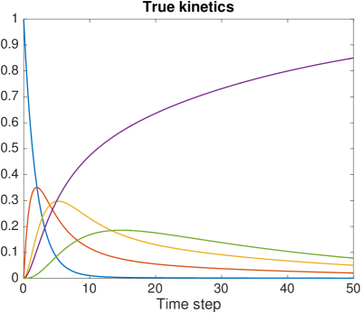
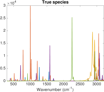
Figure 1: Artificial sequence of first order reactions with five species. The kinetics are shown in the left panel and the species fingerprints (component spectra) are displayed in the right panel. The resulting measurement data are shown in Figure 2 (top).

We let species A be the only educt in the reaction, resulting in the initial concentration vector $h_{0}\mathrel{\mathop{:}}=h(t_{0})=[1,0,0,0,0]^{T}$. If we denote the reaction coefficient matrix corresponding to the above reaction scheme by

$$K=\begin{bmatrix}-0.53&0.02&0.0&0&0.0\\ 0.53&-0.66&0.25&0&0.0\\ 0.0&0.43&-0.36&0&0.1\\ 0.0&0.21&0.0&0&0.0\\ 0.0&0.0&0.11&0&-0.1\end{bmatrix},$$ (9)

the reaction kinetics are given as a function over time by

$$h(t)=[h_{1}(t),\dots,h_{5}(t)]^{T}=e^{Kt}h_{0},$$

as displayed in Figure 1 (left). The corresponding kinetics matrix $H$ is obtained by discretization of $h(t)$ at equidistant steps $t_{0},\dotsc,t_{n-1}$, so that $H=[h(t_{0}),\dotsc,h(t_{n-1})]$.

The five component spectra are constructed by arbitrarily chosen combinations of Lorentzians, inspired by the Raman spectra of various organic compounds. These component spectra were constructed such that each species has at least one characteristic frequency, so that the imposed separability condition (see Section 2.3) is satisfied. The fingerprints constitute the columns of the matrix $W$ (Figure 1 (right)). Visual inspection already reveals that each of the five species has at least one characteristic frequency.

The resulting data matrix is obtained as the product of the kinetic- and spectra matrix, viz. $M=WH$. A visualization of the data matrix $M$ is given in Figure 2 (top).

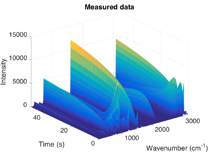
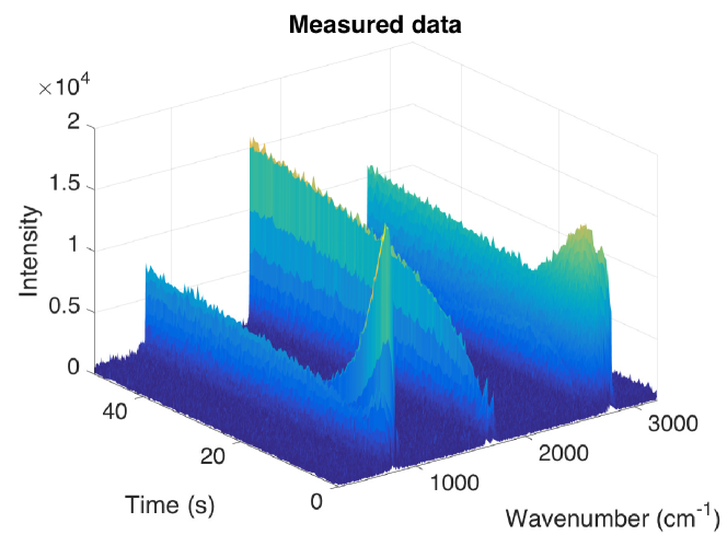
Figure 2: Visualization of the measurement data matrix $M$ for the noiseless, well separated case (top) and an interference-rich, noisy variant (bottom).

4.2 Recovery in the noiseless case

Given the data corresponding to the artificial reaction scheme described in Section 4.1, our goal is now to recover both the component spectra of the five species and the reaction kinetics only from these data, i.e. to recover the matrices $W$ and $H$ using only the data in $M$ without any further information. By construction of the data, we know that $M$ is separable, and we will now apply the methods described in Section 2.3.

The results are displayed in Figure 3, demonstrating that both the reaction kinetics $H$ and all the component spectra are recovered to such a high level of accuracy, that they can hardly be distinguished visually from the original data.

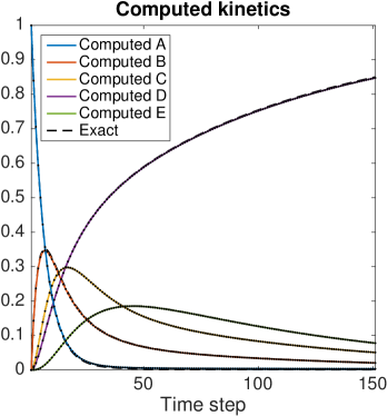
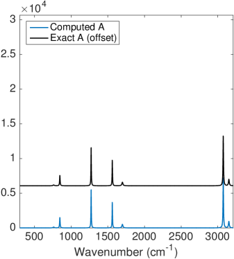
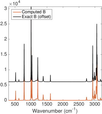
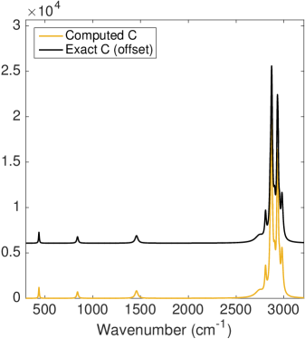
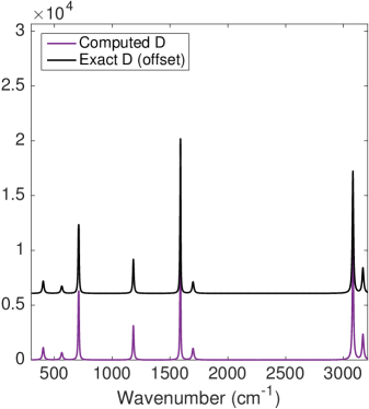
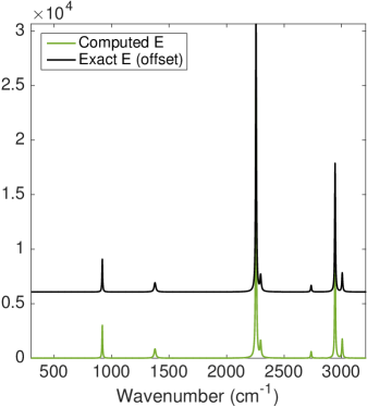
Figure 3: Recovered reaction kinetics (top left) and spectral fingerprints for the noiseless Raman measurements (see Section 4.2). The computed and exact solutions are visually almost indistinguishable.

Nevertheless, the computed factors are not identical to the true factors $W$ and $H$. For the relative errors of $\tilde{W}$ and $\tilde{H}$ we find

$$\frac{\lVert H-\tilde{H}\lVert_{F}}{\lVert H\lVert_{F}}=0.0076,\quad\frac{\lVert W-\tilde{W}\lVert_{F}}{\lVert W\lVert_{F}}=0.0051.$$

Hence the relative error for both the kinetics and the species is less than 1%.

Finally, we will recover the reaction coefficient matrix $K$ from the computed kinetics matrix $\tilde{H}$. Applying the methodology described in Section 3, we obtain

$$\tilde{K}=\begin{bmatrix}-0.5390&0.0349&-0.0082&0.0003&0.0029\\ 0.5272&-0.6580&0.2455&-0.0005&0.0009\\ 0.0020&0.4295&-0.3577&0.0001&0.0995\\ 0.0095&0.1941&0.0100&0.0001&-0.0028\\ 0.0002&-0.0006&0.1104&0.0000&-0.1005\end{bmatrix}.$$

Compared with the true reaction coefficients $K$ in (9), we find that the largest error made in estimating any of the reaction coefficients from the computed kinetics $\tilde{K}$ is $0.0159$, related to the coefficient $k_{12}$.

In summary, we find that all the data that constitute the reaction network described in Section 4.1 have been recovered quite accurately.

4.3 Effect of increased interference

In the model used in the previous section, the bands of the species involved were (visually) well separated from each other. In the other extreme, i.e., if all bands of a species interfere with those of other species, our approach will not be applicable for the recovery of the reaction kinetics and the species fingerprints, as the factors are no longer close to a separable factorization (the term $N_{I}$ in (7) becomes too large). Thus we now consider the case of “modest” interference.

We enforce an increased level of interference among the species by moving all the base points $x_{0}$ in all species towards three focal points (see Figure 4).

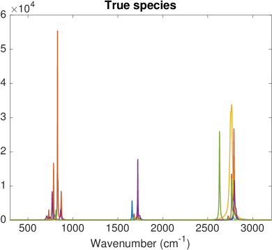
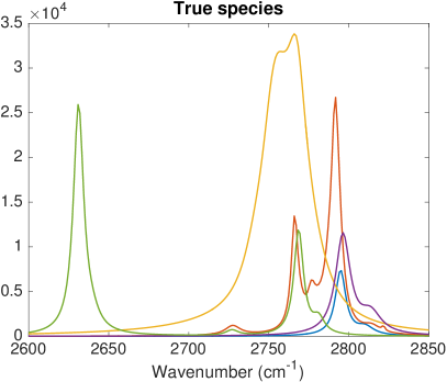
Figure 4: Left: Species fingerprints where the Lorentz bands have been moved closer to each other (compare with Figure 1). Right: Expanded view of the high-frequency region.

The result of Algorithm 1 being applied to these interference-rich data is shown in Figure 5. Because of the increased interference, the computed kinetics deviate slightly from the true ones, but all the species bands have been identified quite satisfactorily. For the relative errors of $\tilde{W}$ and $\tilde{H}$ we find

$$\frac{\lVert H-\tilde{H}\lVert_{F}}{\lVert H\lVert_{F}}=0.063,\quad\frac{\lVert W-\tilde{W}\lVert_{F}}{\lVert W\lVert_{F}}=0.026,$$

so the relative error for both the kinetics and the species spectra is not more than $7\%$ and $3\%$, respectively.

If, however, the bands in the original species spectra are moved even closer to each other, our method will eventually fail to produce a qualitatively good solution.

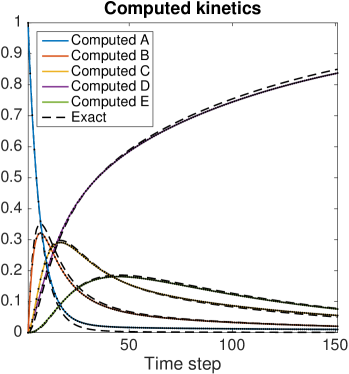
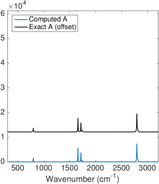
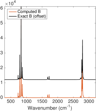
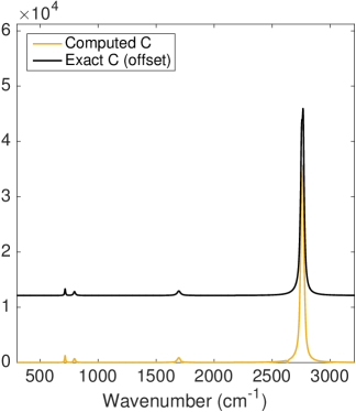
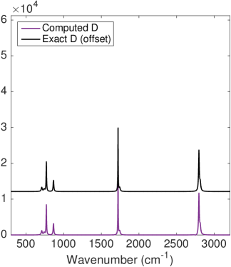
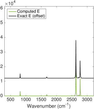
Figure 5: Recovered reaction kinetics (top left) and spectral fingerprints for the case of high interference (see Section 4.3). The computed solutions are still very good approximations to the true solution.

4.4 Recovery under the influence of measurement noise

The data used in the previous section are highly idealized in the sense that they are free of measurement noise. In any practical setting, the experimentally acquired Raman measurements will be contaminated with noise from different sources, such as signal shot noise or background noise (e.g. fluorescence).

We will now simulate the effect of noise added to the measurement matrix $M$ in the sense of (8). We assume that all the noise from different sources taken together resemble additive Gaussian white noise. Overall we disturb the data matrix $M$ according to

$$\tilde{M}=M+\delta\,\text{abs}(N),$$

where the entries of $N\in\mathbb{R}^{m,n}$ are drawn from the normal distribution $\mathcal{N}(0,1)$ and $\delta=0.4$ is the relative noise level. Further we will assume for our noise model, that any constant background has already been removed from the measurement data. In Figure 2 (bottom), we visualize the resulting noisy data $\tilde{M}$.

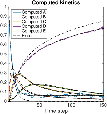
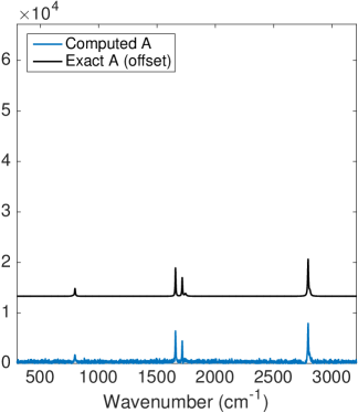
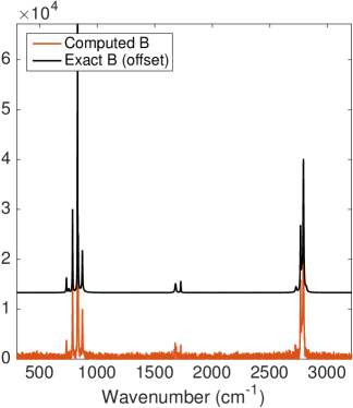
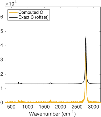
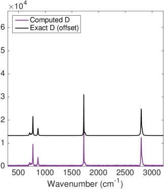
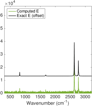
Figure 6: Recovered reaction kinetics (top left) and spectral fingerprints for the noisy Raman measurements (see Section 4.4). The dotted lines in the reaction kinetic show the kinetic corresponding to the extracted reaction coefficients, see Step $6$ in Algorithm 1.

The component spectra and kinetics were recovered as described in Section 3. Figure 6 shows the result of our algorithm applied to the noisy, interference-rich data. Because of the large distance of $W,H$ to being truly separable, the computed kinetics displays some deviations from the true data, but still provides a satisfactory description. Also the computed component spectra show a reasonable agreement with the true spectra.

4.5 Determination of the number of species

In the numerical experiments described above we have always assumed that the number of species is known (here $r=5$). Of course, in practical applications the correct determination of the value of $r$ is one of the greatest challenges. One approach for solving this problem is to use Algorithm 1 for different values of $r$, which yields approximate species $W_{r}$ and kinetics $H_{r}$, and then compute the (relative) data error $\lVert M-W_{r}H_{r}\lVert_{F}/\lVert M\lVert_{F}$.

In the following table we show the data errors for $r=1,2,\dots,7$ and the three experimental setups from Sections 4.2–4.4: noiseless case (first row of the table), increased interference (second), increased interference and measurement noise (third). In each case a significant drop in the data error occurs at the correct number of species, while no significant further reduction of the error is achieved when increasing the number of (suspected) species even further.

$r$	1	2	3	4	5	6	7
Sec. 4.2	0.97294	0.77203	0.18479	0.06055	0.00003	0.00003	0.00003
Sec. 4.3	0.94908	0.68692	0.20209	0.04698	0.00029	0.00029	0.00029
Sec. 4.4	0.83106	0.35383	0.25894	0.12683	0.08169	0.08107	0.08066

Table 1: Relative data fit errors when applying Algorithm 1 to the setups from Sections 4.2–4.4 and different values of $r$.

The results indicate that using the NMF for determining the number of species is an alternative to existing techniques in this context such as singular values of the data matrix. An extensive survey of the latter technique is given in [18].

5 Concluding remarks

We have presented an algorithm for the recovery of component spectra and reaction kinetics from data obtained through time resolved Raman spectroscopy. The key tool we used in our approach is the so-called separability condition in the non-negative matrix factorization (NMF). In terms of the component spectra this condition is approximately satisfied, if each of the species has at least one band in its spectrum that does not interfere too much with the bands of other species. Thus, it is conceptually similar to the classical Rayleigh criterion limit. Our approach combines a standard algorithm for separable NMF (“SNPA”) with a few pre-processing steps for the measurement data. A number of other separable NMF algorithms exist, but we did not yet pursue a detailed comparison among them for the present application. In our numerical study we have demonstrated that the component spectra and reaction kinetics can be recovered with a reasonable quality under modest measurement noise and interference among the component spectra. Whereas in terms of the kinetics the approach currently restricted to a network of first-order or pseudo-first-order reactions, it may equally well applied to other spectroscopic techniques such as IR or NMR spectroscopies.

Acknowledgements

This research was supported by the DFG cluster of excellence “UniCat”.

References

- 1. M. Ando and H.-o. Hamaguchi, “Molecular Component Distribution Imaging of Living Cells by Multivariate Curve Resolution Analysis of Space-Resolved Raman Spectra”. J. Biomed. Opt. 2013. 19(1):011016.
- 2. S. Arora, R. Ge, R. Kannan, and A. Moitra, “Computing a Nonnegative Matrix Factorization—Provably”. In STOC’12—Proceedings of the 2012 ACM Symposium on Theory of Computing, pages 145–161, ACM, New York, 2012.
- 3. G. Balakrishnan, C. L. Weeks, M. Ibrahim, A. V. Soldatova, and T. G. Spiro, “Protein Dynamics from Time Resolved UV Raman Spectroscopy.” Curr. Opin. Struct. Biol. 2008. 18(5):623–629.
- 4. A. Beljebbar, O. Bouché, M. D. Diébold, P. J. Guillou, J. P. Palot, D. Eudes, and M. Manfait, “Identification of Raman Spectroscopic Markers for the Characterization of Normal and Adenocarcinomatous Colonic Tissues.” Crit. Rev. Oncol. Hematol. 2009. 72(3):255–264.
- 5. J. M. Bioucas-Dias, A. Plaza, N. Dobigeon, M. Parente, Q. Du, P. Gader, and J. Chanussot, “Hyperspectral Unmixing Overview: Geometrical, Statistical, and Sparse Regression-Based Approaches”. IEEE J. Sel. Top. Appl. Earth Observations Remote Sensing 2012. 5(2):354–379.
- 6. T.-H. Chan, W.-K. Ma, C.-Y. Chi, and Y. Wang, “A Convex Analysis Framework for Blind Separation of Non-Negative Sources”. IEEE Trans. Signal Process. 2008. 56(10, part 2):5120–5134.
- 7. D. Donoho and V. Stodden, “When Does Non-Negative Matrix Factorization give a Correct Decomposition into Parts?” In S. Thrun, L. Saul, and B. Schölkopf, editors, Advances in Neural Information Processing Systems 16, MIT Press, Cambridge, MA, 2004.
- 8. S. Döpner, P. Hildebrandt, A. G. Mauk, H. Lenk, and W. Stempfle, “Analysis of Vibrational Spectra of Multicomponent Systems. Application to pH-dependent Resonance Raman Spectra of ferricytochrome c”. Spectrochim. Acta, Part A 1996. 52(5):573 – 584.
- 9. N. Gillis, “Robustness Analysis of Hottopixx, a Linear Programming Model for Factoring Nonnegative Matrices”. SIAM J. Matrix Anal. Appl. 2013. 34(3):1189–1212.
- 10. N. Gillis, “Successive Nonnegative Projection Algorithm for Robust Nonnegative Blind Source Separation”. SIAM J. Imaging Sci. 2014. 7(2):1420–1450.
- 11. N. Gillis, “The Why and How of Nonnegative Matrix Factorization”. In Chapman & Hall/CRC Machine Learning & Pattern Recognition, pages 257–291, Chapman and Hall/CRC, 2014.
- 12. N. Gillis and R. Luce, “Robust Near-Separable Nonnegative Matrix Factorization using Linear Optimization”. J. Mach. Learn. Res. 2014. 15:1249–1280.
- 13. N. Gillis and S. A. Vavasis, “Fast and Robust Recursive Algorithms for Separable Nonnegative Matrix Factorization”. IEEE Trans. Pattern Anal. Mach. Intell. 2014. 36(4):698–714.
- 14. R. W. Hendler and R. I. Shrager, “Deconvolutions Based on Singular Value Decomposition and the Pseudoinverse: a Guide for Beginners.” J. Biochem. Biophys. Methods 1994. 28(1):1–33.
- 15. E. Henry and J. Hofrichter, “Singular Value Decomposition: Application to Analysis of Experimental Data”. In Numerical Computer Methods, volume 210 of Methods in Enzymology, pages 129 – 192, Academic Press, 1992.
- 16. A. Kumar, V. Sindhwani, and P. Kambadur, “Fast Conical Hull Algorithms for Near-Separable Non-Negative Matrix Factorization”. ICML 2013. (PART 1):231–239.
- 17. D. D. Lee and H. S. Seung, “Learning the Parts of Objects by Non-Negative Matrix Factorization”. Nature 1999. 401(6755):788–791.
- 18. E. R. Malinkowski, Factor Analysis in Chemistry. John Wiley & Sons, Inc., New York, 3rd edition, 2002.
- 19. K. Neymeyr, M. Sawall, and D. Hess, “Pure Component Spectral Recovery and Constrained Matrix Factorizations: Concepts and Applications”. J. Chemom. 2010. 24(2):67–74.
- 20. M. Ondrias, M. Simpson, and R. Larsen, “Time-Resolved Resonance Raman Spectroscopy”. In J. Laserna, editor, Modern Techniques in Raman Spectroscopy, Wiley, 1996.
- 21. S. K. Sahoo, S. Umapathy, and A. W. Parker, “Time-Resolved Resonance Raman Spectroscopy: Exploring Reactive Intermediates”. Appl. Spectrosc. 2011. 65(10):1087–1115.
- 22. H. Shinzawa, K. Awa, W. Kanematsu, and Y. Ozaki, “Multivariate Data Analysis for Raman Spectroscopic Imaging”. J. Raman Spectrosc. 2009. 40(12):1720–1725.
- 23. A. C. S. Talari, C. A. Evans, I. Holen, R. E. Coleman, and I. U. Rehman, “Raman Spectroscopic Analysis Differentiates Between Breast Cancer Cell Lines”. J. Raman Spectrosc. 2015. 46(5):421–427.
- 24. L. Thomas, “Rank Factorization of Nonnegative Matrices (A. Berman)”. SIAM Rev. 1974. 16(3):393–394.
- 25. M. H. Van Benthem and M. R. Keenan, “Fast Algorithm for the Solution of Large-Scale Non-Negativity-Constrained Least Squares Problems”. J. Chemom. 2004. 18(10):441–450.
- 26. S. A. Vavasis, “On the Complexity of Nonnegative Matrix Factorization”. SIAM J. Optim. 2009. 20(3):1364–1377.
- 27. A. T. Weakley, Warwick, P. C. Temple, T. E. Bitterwolf, and D. E. Aston, “Multivariate Analysis of Micro-Raman Spectra of Thermoplastic Polyurethane Blends Using Principal Component Analysis and Principal Component Regression”. Appl. Spectrosc. 2012. 66(11):1269–1278.
- 28. A. Zhang, W. Zeng, T. M. Niemczyk, M. R. Keenan, and D. M. Haaland, “Multivariate analysis of Infrared Spectra for Monitoring and Understanding the Kinetics and Mechanisms of Adsorption Processes”. Appl. Spectrosc. 2005. 59(1):47–55.