Quantum Zeno effect and non-Markovianity in a three-level system

Abstract

We study the coexistence of the quantum Zeno effect and non-Markovianity for a system decaying in a structured bosonic environment and subject to a control field. The interaction with the environment induces decay from the excited to the ground level, which, in turn, is coherently coupled to another meta-stable state. The control of the strength of the coherent coupling between the stable levels allows the engineering of both the dissipation and of the memory effects, without modifying neither the system-reservoir interaction, nor environmental properties. We use this framework in two different parameter regimes corresponding to fast (bad cavity limit) and slow dissipation (good cavity limit) in the original, un-controlled qubit system. Our results show a non-monotonic behavior of memory effects when increasing the effectiveness of the Zeno-like freezing. Moreover, we identify a new source of memory effects which allows the persistence of non-Markovianity for long times while the excited state has already been depleted.

I Introduction

How can a flying arrow be moving, if at any instant of time when it is observed, it is seen in some place, stationary? This was one of the paradoxes of Zeno of Elea (laertius, ), an ancient Greek philosopher. A little bit over two thousand years later, von Neumann’s reduction postulate neumann laid the foundation for a similar effect in quantum mechanics. Namely, if a quantum measurement collapses the state of a quantum system to a state in the measurement basis, this process is repeated $N$ times a second and $N$ is let to tend to infinity, the motion of the system is prevented. The quantum phenomenon was named the quantum Zeno effect in sudarmisra and has been been studied in several earlier works, see beskow ; khalfin ; kurizki1 ; kurizki2 ; zenoreview ; zenoent1 ; zenoent2 and references therein. Besides frequent measurements, a strong coupling to an external, control system or level can also prevent the original system of interest from evolving in time kraus ; watchdog . Loosely speaking the control system is continuously measuring or gazing at the system of interest and thereby preventing its dynamics. This effect is called dominated evolution or the watchdog effect and is the one that we will study in this paper from the point of view of non-Markovianity and information flow.

Markovian dynamics is generally understood to be describable by the semigroup evolution and Lindblad equation BREUERBOOK . However, Markovian dynamics is always an approximation and not necessarily valid for all systems nor environments. Therefore, understanding non-Markovian memory effects is an important aspect when studying open system dynamics in general. Different approaches to define and quantify non-Markovian dynamics based on different physical or mathematical quantities have been actively developed in recent years wolf ; NMprl ; rivas ; mani ; determinant ; LFS , see also recent reviews NMreviewblp ; NMreviewhuelga . These quantifiers are based on the non-monotonicity of some kind of information flow towards the system, and have been compared and classified in mani ; com ; comp1 ; compa2 ; compar3 ; compare4 ; compared5 .

Here, we are interested in describing the modifications of the information flow due to the control field induced freezing of the decay, and, more generally in how to control the Zeno effect and non-Markovianity, and what is their interplay. For this purpose, we study a two-level system interacting with a zero-temperature bosonic environment. In this qubit system, the coupling strength to the environment and environmental properties, such as spectral density, define whether the qubit dynamics displays memory effects or not. However, adding a coherent coupling to an auxiliary third level allows to control the excited state dynamics – displaying Zeno-effect– and also to engineer the memory effects. The paper is organized in the following way. Section II describes the system under study and Sec. III introduces briefly the basic aspects of the used measure for non-Markovianity. The central results are presented in Sec. IV and Sec. V concludes.

II Model and Dynamics

Our system is schematically described in Fig 1. The total Hamiltonian of the system and the environment in the rotating wave approximation can be written as

$$H_{tot}=H_{S}+H_{E}+H_{int}+H_{C}$$ (1)

where

$$H_{S} =\omega_{a}\left|a\right\rangle\left\langle a\right|+\omega_{b}\left|b\right\rangle\left\langle b\right|+\omega_{m}\left|m\right\rangle\left\langle m\right|$$ (2)

$$H_{E} =\sum_{j}\omega_{j}a_{j}^{\dagger}a_{j}$$ (3)

$$H_{int} =\sum_{j}g^{*}_{j}\left|b\right\rangle\left\langle a\right|a^{\dagger}_{j}+g_{j}\left|a\right\rangle\left\langle b\right|a_{j},$$ (4)

$$H_{C} =g(\left|b\right\rangle\left\langle m\right|e^{i\Delta_{1}t}+\left|m\right\rangle\left\langle b\right|e^{-i\Delta_{1}t})$$ (5)

where $a^{\dagger}$ and $a$ are the bosonic creation and annihilation operators, $g_{j}$ and $g$ the coupling strength to the $j$th mode of the environment and the level $\left|m\right\rangle$ respectively, $\omega_{a},\hskip 2.0pt\omega_{b},\hskip 2.0pt\omega_{m}$ the frequencies of the levels $|a\rangle,|b\rangle,|m\rangle$, $\omega_{j}$ are the frequencies of the environment modes and

$$\Delta_{0} =\omega_{a}-\omega_{b}$$

$$\Delta_{1} =\omega_{m}-\omega_{b}.$$ (6)

Notice that the level $|m\rangle$ is neither directly coupled with the environment nor with level $|a\rangle$; it enters the dynamics for control purposes only. From here on, we will work in the interaction picture defined by the free Hamiltonian. The interaction Hamiltonian becomes

$$H^{(i)}= \sum_{j}g_{j}\left|a\right\rangle\left\langle b\right|a_{j}e^{-i(\omega_{j}-\Delta_{0})t}+g^{*}_{j}\left|b\right\rangle\left\langle a\right|a^{\dagger}_{j}e^{i(\omega_{j}-\Delta_{0})t}$$

$$+g(\left|b\right\rangle\left\langle m\right|+\left|m\right\rangle\left\langle b\right|).$$ (7)

For simplicity we consider the case of only one excitation in the whole system initially, with initially empty environment modes. This means that the initial state can be written as

$$\left|\psi(0)\right\rangle=(\alpha_{0}\left|a\right\rangle+\beta_{0}\left|b\right\rangle+\mu_{0}\left|m\right\rangle)\otimes\left|\{0\}\right\rangle.$$ (8)

Because the excitation number is conserved, the state at any later time is

$$\left|\psi(t)\right\rangle= (\alpha(t)\left|a\right\rangle+\beta(t)\left|b\right\rangle+\mu(t)\left|m\right\rangle)\otimes\left|\{0\}\right\rangle$$

$$+\sum_{j}\beta_{j}(t)\left|b\right\rangle\otimes\left|1_{j}\right\rangle+\sum_{j}\mu_{j}(t)\left|m\right\rangle\otimes\left|1_{j}\right\rangle,$$ (9)

where $\left|1_{j}\right\rangle=a^{\dagger}_{j}\left|\{0\}\right\rangle$ means an excitation in the $j$th mode in the environment. To find the form of the coefficients we solve the Schrödinger equation in the Appendix. For the bosonic environment, we use a Lorentzian spectral density function

$$J(\omega)=\Omega_{0}^{2}\frac{\lambda}{\pi((\omega-\Delta_{0})^{2}+\lambda^{2})},$$ (10)

where $\Omega_{0}^{2}=\frac{\lambda\gamma}{2}$. Varying the width of the Lorentzian allows us to use a good and a bad cavity limits – having $\gamma/\lambda\gg 1$ ($\gamma/\lambda\ll 1$) corresponds to good (bad) cavity limit. The solution of the Schrödinger equation is fairly complicated but we can in quite a straightforward manner use it to study the dynamics of the system numerically. In the following sections, we first introduce the BLP-measure for quantifying the non-Markovianity and then present the results.

Figure 1: Sketch of our model: A two-level system, with excited and ground states $|a\rangle$ and $|b\rangle$, respectively, interacts with a zero-temperature bosonic environment E, while the lower level $|b\rangle$ is coherently coupled to an external level $|m\rangle$ with strength $g$. Such a coupling, enables the control of the $|a\rangle\longrightarrow|b\rangle$ decay and of memory effects.

III Non-Markovianity

In general, quantum channels are one-parameter families $\{\Phi_{t}\}_{t>0}$ of completely positive, trace preserving (CPTP) maps. Each member $\Phi_{t}$ of the family evolves a quantum state from the initial time $t=0$ to time $t>0$, denoted

$$\rho(t)=\Phi_{t}\rho(0).$$ (11)

The set of quantum states is the set of positive operators with unit trace and can be endowed with a metric called the trace distance $D(\cdot,\cdot)$ induced by the trace norm $||\cdot||_{1}$ by the following formula

$$D(\rho_{1},\rho_{2})=\frac{1}{2}||\rho_{1}-\rho_{2}||_{1}.$$ (12)

It turns out fuchsvdg that this metric is related to the optimal probability $P_{max}$ of correctly distinguishing two unknown quantum states from each other. The relation is

$$P_{max}(\rho_{1},\rho_{2})=\frac{1}{2}(1+D(\rho_{1},\rho_{2})).$$ (13)

This gives an operational meaning to the trace distance as a measure of distinguishability of quantum states. CPTP maps are contractions for the trace distance ruskai , which means that quantum channels tend to decrease the distuinguishability of quantum states. We defined channels as families of CPTP maps that map the input states from initial time $t=0$ to some later time $t$. If we study the intermediate maps $\Phi_{t_{1},t_{2}}$, where $0<t_{1}<t_{2}$, which evolve the state from time $t_{1}$ to time $t_{2}$, the CPTP property need not hold anymore. This means that locally in time, the trace distance can increase, but never above the original value at time $t=0$.

Interpreting the decrease of trace distance as information flowing out and increase of the trace distance as a refocusing of information onto the system, we arrive at the Breuer, Laine, Piilo (BLP) measure of non-Markovianity NMprl defined by

$$\mathcal{N}_{\textrm{BLP}}=\underset{\rho_{1}(0),\rho_{2}(0)}{\text{sup}}\int_{\sigma(\rho_{1}(t),\rho_{2}(t))>0}\sigma(\rho_{1}(t),\rho_{2}(t))\hskip 2.0pt\text{d}t,$$ (14)

where

$$\sigma(\rho_{1}(t),\rho_{2}(t))=\frac{dD(\rho_{1}(t),\rho_{2}(t))}{dt}.$$ (15)

The measure takes as an input a pair of initial states $\rho_{1}(0)$ and $\rho_{2}(0)$, monitors the dynamics of their trace distance and adds up all the possible increases in time. This is maximized over all possible choices of the initial pairs giving a value that describes the non-Markovianity of a quantum channel.

The maximization over all possible pairs of initial states seems cumbersome, but can be simplified optpairs ; univnm . The idea is, that since the state pairs enter the measure only as their difference, the important quantity is actually the direction in the set of quantum states. Many different state pairs give the same direction, meaning that their difference is the same up to a constant. Also, any direction (which here means a traceless hermitian matrix) can be written as a difference of two quantum states univnm . This simplifies the maximization procedure by removing the need to search over all possible state combinations and replacing it with a search over all possible directions. We use this method in our numerical work, which is presented in the following section.

IV Results

Since the external level $\left|m\right\rangle$ is introduced only to control the dynamics of the original two–level system, we restrict the optimization to initial states where the external level $|m\rangle$ is empty. This means that we are interested in initial states with $\mu_{0}=0$, which in turn means that the states are described by the parameters $\alpha_{0}$ and $\beta_{0}$ alone. This implies that in the initial state density matrix (see the appendix), only the upper left 2x2 block is non-zero, which enables us to represent the interesting ones using the Bloch sphere, i.e in the form

$$\rho_{0}=\frac{1}{2}(\sigma_{0}+\vec{r}\cdot\vec{\sigma}),$$ (16)

where $||\vec{r}||\leq 1$ and $\sigma_{i}$ are the Pauli matrices. The matrix describing the actual state of our system is the form $\rho_{0}$ above, appropriately padded with zeros to make the density matrix 3x3. We find the value of the measure by exploiting the direction argument in the following way. First we choose a finite integration time, $\lambda t=20$, for which the evolution of the system is monitored. A random point and its antipodal point from the Bloch sphere are chosen as the state pair for which the value of the trace distance integral is calculated f. This number is stored and the process repeated for a desired number of times (in our case 500 samples). The numbers are normalized to range from 0 to 1. This way we get an approximate map of how the different directions on the Bloch sphere behave in terms of the BLP measure.

We study two different regimes – corresponding to a bad and a good cavity – by appropriately choosing the parameter $\gamma$ of the spectral density defined in equation (10). In particular, we take $\gamma=\frac{\lambda}{10}$ to describe a bad cavity and $\gamma=10\lambda$ for a good cavity. Also the coupling strength $g$ to the external level is varied between 0 and $100\lambda$. In all but one of the cases that we studied, the values of the measure were distributed like in Fig. 2, meaning that the maximizing direction is the one through the north and the south pole, corresponding to the initial state pair

$$\rho_{1}(0) =|a\rangle\langle a|$$ (17)

$$\rho_{2}(0) =|b\rangle\langle b|.$$ (18)

In the one exception, which was the good cavity with zero coupling to the external level, the maximizing pair could have been taken as any pair from the equator.

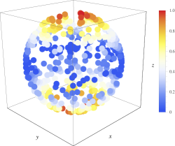
Figure 2: (Color on-line): Bloch sphere representation of the directions and the corresponding value for the BLP measure with parameter values $\gamma=10\lambda,\hskip 2.0ptg=10\lambda$. Red means high and blue low value for the measure. Note that in the figure, the value of the measure has been normalized so that $0\leqslant\mathcal{N}_{\textrm{BLP}}\leqslant 1$.

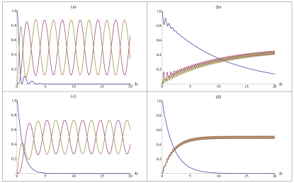
Figure 3: (Color on-line): Population of the excited state (blue), ground state (yellow) and the external level (purple) in the good (a-b) ($\gamma=10\lambda$) and bad (c-d) cavity ($\gamma=\frac{\lambda}{10}$) case. In (a) we have used $g=\lambda$ and in (b) $g=10\lambda$. Similarly in (c) $g=\frac{\lambda}{10}$ and in (d) $g=\lambda$. In all of these cases, we took an initially excited system prepared in $|a\rangle$.

In Figure 3, we plot the dynamics of the population of the different levels to show how increasing the coupling $g$ affects the dynamics of the system both in good and bad cavity cases. In Figure 3 (a), which corresponds to good cavity with weak coherent coupling between the two lower levels, the excited level population reaches zero followed by a few revival cycles typical for non-Markovian behaviour. The populations of the lower levels keep oscillating with quite a large amplitude and small frequency. When the coupling $g$ is increased, Fig. 3 (b), the Zeno effect influences the dynamics making the dissipation from the excited state slower. This also decreases the oscillation amplitudes of the populations of the lower levels, and at the same time frequency is higher due to the increased value of $g$. For the bad cavity case in Fig. 3 (c) and (d) the situation looks qualitatively similar except that the excited state decreases monotonically in contrast to oscillations displayed by the good cavity case. Due to the monotonic decrease in the excited state population, one would be tempted to conclude that for the bad cavity case the dynamics is Markovian. However, this is not true and eventually it turns out that memory effects influence the dynamics in quite a long time scale even beyond the point when the excited state has already been depleted of population.

The long term influence of the memory effects is displayed in Fig.  4, which shows the trace distance dynamics for the good cavity case for weak and strong coupling. For the weak coupling, when the Zeno effect does not yet dominate the dynamics, the trace distance keeps oscillating with quite a high amplitude without damping beyond the point when the excited state is already depleted. This looks peculiar since in this regime the system and the environment do not exchange energy anymore. However, this can be explained when looking at the equations of motions and solutions for the various probability amplitudes (for full details, see the Appendix, where an analytic solution of the equations of motion is presented). First, the equation for the excited state amplitude $\alpha$ is of the form

$$\dot{\alpha}(t)=-\int_{0}^{t}f(t-t_{1})\cos(g(t-t_{1}))\alpha(t_{1})\text{d}t_{1}\,.$$ (19)

By increasing $g$ the kernel of the integral keeps oscillating faster and faster, so that the integral itself decreases, giving rise to a freezing of the excited state amplitude. In general, for an initial state with $\beta=\mu=0$, the open system state at time $t$, is,

$$\rho(t)=\begin{pmatrix}|\alpha(t)|^{2}&0&0\\ 0&\sum\limits_{j}|\beta_{j}(t)|^{2}&\sum\limits_{j}\beta_{j}(t)\mu^{*}_{j}(t)\\ 0&\sum_{j}\beta^{*}_{j}(t)\mu_{j}(t)&\sum\limits_{j}|\mu_{j}(t)|^{2}\end{pmatrix}.$$ (20)

The time evolution of the populations of the two lower levels, also in the regime when excited state is depleted, are given by

$$\sum_{j}|\mu_{j}(t)|^{2}=\Omega_{0}^{2} \int_{0}^{t}\text{d}t_{1}\int_{0}^{t}\text{d}t_{2}e^{-\lambda|t_{1}-t_{2}|}\alpha(t_{1})\alpha^{*}(t_{2})$$

$$\times\sin(g(t-t_{1}))\sin(g(t-t_{2}))$$ (21)

$$\sum_{j}|\beta_{j}(t)|^{2}=\Omega_{0}^{2} \int_{0}^{t}\text{d}t_{1}\int_{0}^{t}\text{d}t_{2}e^{-\lambda|t_{1}-t_{2}|}\alpha(t_{1})\alpha^{*}(t_{2})$$

$$\times\cos(g(t-t_{1}))\cos(g(t-t_{2})).$$ (22)

The important point to notice here is that even though after some time $\alpha=0$, the $\sin$ and $\cos$ terms depend on $t$, and therefore also the values of the integrals depend on time and so do the populations. This is ultimately due to the coupling between the lower levels. However, it makes a large difference, in terms of information flow and non-Markovianity, whether the lower levels are coupled without prior dissipation [see Eqs. (30-31) in the Appendix], or can enter the coupling cycle after some population has decayed from the excited state. As the equations above show, due to the memory effects the lower level populations depend on the past values of the excited state amplitude, and not only on the instantaneous ones, thus explaining the long time survival of oscillations in the trace distance.

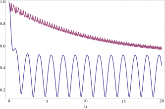
Figure 4: (Color on-line): The behavior of the trace distance of the maximizing pair in the good cavity case with $g=\lambda$ (blue) and $g=10\lambda$ (yellow).

The trace distance measure for non-Markovianity is generally associated to a back-flow of information into the open system, so that a question naturally arises: Where does the information come from in this case? To answer, let us consider the total system state as a function of time, for initial states with $\beta=\mu=0$, and after the excited state has decayed, $\alpha=0$. It is

$$\left|\psi(t)\right\rangle=\sum_{j}\beta_{j}(t)\left|b\right\rangle\otimes\left|1_{j}\right\rangle+\sum_{j}\mu_{j}(t)\left|m\right\rangle\otimes\left|1_{j}\right\rangle.$$ (23)

Taking a trace over the system shows that the environmental state does not change anymore. However, the coherences within the total system state do change and also the system-environment correlations. It is this change of the correlations which is ultimately responsible for long-term memory effects here. Note that these memory effects are induced by coherently coupling the second lower to the ground state. In other words, in this case, the origin of the memory effects is not in the engineering of the environment properties, nor in changing the system-environment coupling. Instead, it is related to manipulating the global coherences in the total system, which is enabled by the coherent coupling.

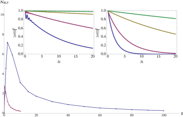
Figure 5: (Color on.line): The BLP measure as a function of the coupling strength $g$ to the external level. The blue line is for the good cavity regime $(\gamma=10\lambda)$, while purple refers to the bad cavity case $(\gamma=\frac{\lambda}{10})$. The left inset displays the population of the excited state as a function of time with $g=10\lambda,20\lambda,50\lambda,100\lambda$ (from bottom to top) in the good cavity case. The right inset gives the same in the bad cavity case with $g=\lambda,2\lambda,5\lambda,10\lambda$ (from bottom to top).

Let us now turn the attention to the amount of memory effects when increasing the coupling $g$ and Zeno effect. The BLP measure for the good and bad cavity cases as a function of $g$ is displayed in Fig. 5. The memory effects are more pronounced in the good cavity case than in the bad one. However, in both of the cases the amount of memory effects behaves in non-monotonic way. There is a specific value of $g$ where the maximum is reached. This is inherently related to the fact that within the current system, there are two sources of non-Markovianity. Small-time oscillations in the excited state population and long-time persistent oscillations for the ground state populations. When $g=0$, the bad cavity case does not display memory effects whereas the good cavity case displays minor memory effects. Increasing the coupling constant $g$ induces the ground state oscillations with increasing amplitude making the memory effects more prominent. However, at the same time the Zeno-effect tends to freeze excited state population and as a consequence, reduce the ground state oscillations. Therefore, due to the these competing effects, a specific value of $g$ allows to maximize the memory effects and beyond this point Zeno-effect begins to dominate reducing non-Markovianity. See also the insets in Fig. 5 displaying in detail how Zeno-effect appears freezing the excited state dynamics.

V Conclusions

We have studied both Zeno-effect and non-Markovianity in a three-level system. The results show that the same coupling, which is used to freeze the excited state dynamics, also induces non-Markovianity in non-trivial manner. In particular, the memory effects persist for long times when the system and the environment do not exchange energy anymore. As a matter of fact, there is a competition between the strength of the memory effects and freezing of the excited state population. As a consequence, the amount of non-Markovianity behaves in non-monotonic way in terms of the strength of Zeno effect. Eventually, when the population dynamics of the excited state completely freezes, memory effects disappear. However, we have revealed a parameter regime which displays a rich interplay between Zeno and non-Markovian dynamics and this also identifies a novel source for memory effects whose origin is inherently independent of the properties of the environment.

Aknowledgement We acknowledge support from EU project QuProCS (Grant Agreement 641277) and from the Magnus Ehrnrooth foundation.

Appendix

Let us assume that initially there is only one excitation in the system and that the environment modes are empty. Then the initial state can be written as

$$\left|\psi(0)\right\rangle=(\alpha_{0}\left|a\right\rangle+\beta_{0}\left|b\right\rangle+\mu_{0}\left|m\right\rangle)\otimes\left|\{0\}\right\rangle.$$ (24)

Since the excitation number is conserved, the state at any later time is

$$\left|\psi(t)\right\rangle= (\alpha(t)\left|a\right\rangle+\beta(t)\left|b\right\rangle+\mu(t)\left|m\right\rangle)\otimes\left|\{0\}\right\rangle$$

$$+\sum_{j}\beta_{j}(t)\left|b\right\rangle\otimes\left|1_{j}\right\rangle+\sum_{j}\mu_{j}(t)\left|m\right\rangle\otimes\left|1_{j}\right\rangle,$$ (25)

where $\left|1_{j}\right\rangle=a^{\dagger}_{j}\left|\{0\}\right\rangle$ is the state with one excitation in the $j$th mode of the environment. Equivalently, the state in density matrix form $\rho(t)$ after taking the partial trace over the environmental degrees of freedom from equation (Appendix) is

$$\begin{pmatrix}|\alpha(t)|^{2}&\alpha(t)\beta^{*}(t)&\alpha(t)\mu^{*}(t)\\ \alpha^{*}(t)\beta(t)&|\beta(t)|^{2}+\sum\limits_{j}|\beta_{j}(t)|^{2}&\beta(t)\mu^{*}(t)+\sum\limits_{j}\beta_{j}(t)\mu^{*}_{j}(t)\\ \alpha^{*}(t)\mu(t)&\beta^{*}(t)\mu(t)+\sum_{j}\beta^{*}_{j}(t)\mu_{j}(t)&|\mu(t)|^{2}+\sum\limits_{j}|\mu_{j}(t)|^{2}\end{pmatrix}.$$ (26)

Schrödinger equation now leads to the following set of coupled differential equations for the coefficients

$$\dot{\beta}(t) =-ig\mu(t)$$ (27)

$$\dot{\mu}(t) =-ig\beta(t)$$ (28)

$$\dot{\alpha}(t) =-i\sum_{j}g_{j}e^{-i(\omega_{j}-\Delta_{0})}\beta_{j}(t)$$ (29)

$$\dot{\beta}_{j}(t) =-ig^{*}_{j}e^{i(\omega_{j}-\Delta_{0})}\alpha(t)-ig\mu_{j}(t)$$ (30)

$$\dot{\mu}_{j}(t) =-ig\beta_{j}(t).$$ (31)

From the above equations we can directly solve for two coefficients

$$\beta(t) =\beta_{0}\cos(gt)-i\mu_{0}\sin(gt)$$ (32)

$$\mu(t) =\mu_{0}\cos(gt)-i\beta_{0}\sin(gt).$$ (33)

To proceed, we use the following transformation to decouple equations (30) and (31)

$$l_{j}(t)=\frac{\beta_{j}(t)+\mu_{j}(t)}{\sqrt{2}}\quad\quad r_{j}(t)=\frac{\beta_{j}(t)-\mu_{j}(t)}{\sqrt{2}},$$ (34)

which leads to differential equations that can be integrated directly

$$\dot{l}_{j}(t) =-i\frac{g^{*}_{j}}{\sqrt{2}}e^{i(\omega_{j}-\Delta_{0})t}\alpha(t)-igl_{j}(t)$$ (35)

$$\dot{r}_{j}(t) =-i\frac{g^{*}_{j}}{\sqrt{2}}e^{i(\omega_{j}-\Delta_{0})t}\alpha(t)+igr_{j}(t).$$ (36)

Integrating the above equations and solving for $\beta_{j}$ and $\mu_{j}$ from equation (34) yields

$$\beta_{j}(t)=-ig^{*}_{j}\int_{0}^{t}\text{d}t_{1}e^{i(\omega_{j}-\Delta_{0})t_{1}}\cos(g(t-t_{1}))\alpha(t_{1})$$ (37)

$$\mu_{j}(t)=-ig^{*}_{j}\int_{0}^{t}\text{d}t_{1}e^{i(\omega_{j}-\Delta_{0})t_{1}}\sin(g(t-t_{1}))\alpha(t_{1}).$$ (38)

Now we can insert the solution for $\beta_{j}$ to the differential equation for $\alpha$, which leads to

$$\dot{\alpha}(t)=-\int_{0}^{t}\sum_{j}|g_{j}|^{2}e^{-i(\omega_{j}-\Delta_{0})(t-t_{1})}\cos(g(t-t_{1}))\alpha(t_{1})\text{d}t_{1}.$$ (39)

To proceed from here we approximate the state of the environment with a continuous distribution of modes, whose spectral density is given by the function $J(\omega)$. The approximation amounts to the replacement

$$\sum_{j}|g_{j}|^{2}e^{-i(\omega_{j}-\Delta_{0})(t-t_{1})}\rightarrow \int_{-\infty}^{\infty}J(\omega)e^{-i(\omega-\Delta_{0})(t-t_{1})}\text{d}\omega$$

$$\equiv f(t-t_{1}).$$ (40)

With this, the equation for $\alpha$ becomes

$$\dot{\alpha}(t)=-\int_{0}^{t}f(t-t_{1})\cos(g(t-t_{1}))\alpha(t_{1})\text{d}t_{1}.$$ (41)

Let us assume that the form of the spectral density is a Lorentzian

$$J(\omega)=\Omega_{0}^{2}\frac{\lambda}{\pi((\omega-\Delta_{0})^{2}+\lambda^{2})},$$ (42)

where $\Omega_{0}^{2}=\frac{\lambda\gamma}{2}$. The form of the spectral density function could be almost anything, but this choice makes the calculations fairly simple. By controlling the parameters $\gamma$ and $\lambda$, which are basically the height and width of the Lorentzian, we can switch between Markovian and non-Markovian behavior of the system. We can now evaluate the integral in equation (Appendix) and obtain

$$f(t-t_{1})=\Omega_{0}^{2}e^{-\lambda|t-t_{1}|}.$$ (43)

Let us denote

$$F(t-t_{1})=\Omega_{0}^{2}e^{-\lambda|t-t_{1}|}\cos(g(t-t_{1}))$$ (44)

and denote $t-t_{1}=\tau$. Then the Laplace transform of $F$ is

$$\tilde{F}(s)=\int_{0}^{\infty}e^{-s\tau}F(\tau)\text{d}\tau=\Omega_{0}^{2}\frac{s+\lambda}{(s+\lambda)^{2}+g^{2}}.$$ (45)

Laplace transforming the differential equation for $\alpha$ we get

$$s\tilde{\alpha}(s)-\alpha_{0}=-\tilde{F}(s)\tilde{\alpha}(s),$$ (46)

which combined with equation (45) leads to

$$\tilde{\alpha}(s)=\alpha_{0}\frac{(s+\lambda)^{2}+g^{2}}{s(s+\lambda)^{2}+s(\Omega_{0}^{2}+g^{2})+\Omega_{0}^{2}\lambda}.$$ (47)

Denoting the three roots of the denominator with $s_{i}$ and taking the inverse transform, we solve for

$$\alpha(t)= \alpha_{0}\big{(}\frac{(s_{1}+\lambda)^{2}+g^{2}}{(s_{1}-s_{2})(s_{1}-s_{3})}e^{s_{1}t}+\frac{(s_{2}+\lambda)^{2}+g^{2}}{(s_{2}-s_{1})(s_{2}-s_{3})}e^{s_{2}t}$$

$$+\frac{(s_{3}+\lambda)^{2}+g^{2}}{(s_{3}-s_{1})(s_{3}-s_{2})}e^{s_{3}t}\big{)}.$$ (48)

With this solution and after some simplifications we finally solve for the remaining coefficients in the density matrix

$$\sum_{j}|\mu_{j}(t)|^{2}=\Omega_{0}^{2} \int_{0}^{t}\text{d}t_{1}\int_{0}^{t}\text{d}t_{2}e^{-\lambda|t_{1}-t_{2}|}\alpha(t_{1})\alpha^{*}(t_{2})$$

$$\times\sin(g(t-t_{1}))\sin(g(t-t_{2}))$$ (49)

$$\sum_{j}|\beta_{j}(t)|^{2}=\Omega_{0}^{2} \int_{0}^{t}\text{d}t_{1}\int_{0}^{t}\text{d}t_{2}e^{-\lambda|t_{1}-t_{2}|}\alpha(t_{1})\alpha^{*}(t_{2})$$

$$\times\cos(g(t-t_{1}))\cos(g(t-t_{2}))$$ (50)

$$\sum_{j}\mu^{*}_{j}(t)\beta_{j}(t)=\Omega_{0}^{2} \int_{0}^{t}\text{d}t_{1}\int_{0}^{t}\text{d}t_{2}e^{-\lambda|t_{1}-t_{2}|}\alpha(t_{1})\alpha^{*}(t_{2})$$

$$\times\cos(g(t-t_{1}))\sin(g(t-t_{2})).$$ (51)

References

- (1) Laertius, Diogenes, Lives and Opinions of Eminent Philosophers IX (about 230 CE).
- (2) J. von Neumann, Mathematische Grundlagen der Quantenmechanik, Springer (1932).
- (3) E. C. G. Sudarshan, B. Misra, The Zeno’s paradox in quantum theory, J. Math. Phys. 18, 4 (1977).
- (4) A. Beskow, J. Nilsson, Concept of wave function and the irreducible representations of the Poincare group. II. Unstable systems and the exponential decay law, Ark. Fys. 34 (1967).
- (5) L. A., Khalfin, Zh. Eksp. Teor. Fiz. Pisma Red. 8, 106 (1968) (English transl. JETP Letters 8, 65 (1968)).
- (6) A. G. Kofman, G. Kurizki, Acceleration of quantum decay processes by frequent observations, Nature 405, 546-550 (2000).
- (7) A. G. Kofman, G. Kurizki, Universal Dynamical Control of Quantum Mechanical Decay: Modulation of the Coupling to the Continuum, Phys. Rev. Lett. 87, 270405 (2001).
- (8) P. Facchi, S. Pascazio, Quantum Zeno and inverse quantum Zeno effects Prog. Optics 42, 3 (2001).
- (9) S. Maniscalco, F. Francica, R. L. Zaffino, N. Lo Gullo, F. Plastina, Protecting Entanglement via the Quantum Zeno Effect, Phys. Rev. Lett. 100, 090503 (2008).
- (10) F. Francica, F. Plastina, S. Maniscalco, Quantum Zeno and anti-Zeno effects on quantum and classical correlations, Phys. Rev. A 82, 052118 (2010).
- (11) K. Kraus, Measuring processes in quantum mechanics I. Continuous observation and the watchdog effect Found. Phys. 11, 7 (1981).
- (12) V. P. Belavkin, P. Staszewski, Nondemolition observation of a free quantum particle, Phys. Rev. A 45, 1347 (1992).
- (13) H.-P. Breuer, F. Petruccione, The Theory of Open Quantum Systems, Oxford University Press (2007).
- (14) M. M. Wolf, J. Eisert, T. S. Cubitt, J. I. Cirac, Assessing non-Markovian quantum dynamics, Phys. Rev. Lett. 101, 150402 (2008).
- (15) H.-P. Breuer, E.-M. Laine, J. Piilo, Measure for the degree of non-Markovian behavior of quantum processes in open systems, Phys. Rev. Lett. 103, 210401 (2009).
- (16) Á. Rivas,S. F. Huelga, M. B. Plenio, Entanglement and non-Markovianity of quantum evolutions, Phys. Rev. Lett. 105, 050403 (2010).
- (17) D. Chruściński, S. Maniscalco, Degree of non-Markovianity of quantum evolution, Phys. Rev. Lett. 112, 120404 (2014).
- (18) S. Lorenzo, F. Plastina, M. Paternostro, Geometrical characterization of non-Markovianity, Phys. Rev. A 88, 020102 (2013).
- (19) S. Luo, S. Fu, H. Song, Quantifying non-Markovianity via correlations, Phys. Rev. A 86, 044101 (2012).
- (20) H.-S. Zeng, N. Tang, Y.-P. Zheng, and G. Y.Wang, Equivalence of the measures of non-Markovianity for open two-level systems, Phys. Rev. A 84, 032118 (2011).
- (21) D. Chruściński, A. Kossakowski, Á. Rivas, Measures of non-Markovianity: Divisibility versus backflow of information, Phys. Rev. A 83, 052128 (2011).
- (22) P. Haikka, J. D. Cresser, and S. Maniscalco, Comparing different non-Markovianity measures in a driven qubit system, Phys. Rev. A 83, 012112 (2011).
- (23) M. Jiang and S. Luo, Comparing quantum Markovianities: Distinguishability versus correlations, Phys. Rev. A 88, 034101 (2013).
- (24) T. J. G. Apollaro, S. Lorenzo, C. Di Franco, F. Plastina, M. Paternostro, Competition between memory-keeping and memory-erasing decoherence channels, Phys. Rev. A 90, 012310 (2014).
- (25) S. Wissmann, H.-P. Breuer, B. Vacchini, Generalized trace-distance measure connecting quantum and classical non-Markovianity, Phys. Rev. A 92, 042108 (2015).
- (26) H.-P. Breuer, E.-M. Laine, J. Piilo, B. Vacchini, Non-Markovian dynamics in open quantum systems arXiv:1505.01385 (2015).
- (27) Á. Rivas, S. F. Huelga, M. B. Plenio, Quantum non-Markovianity: characterization, quantification and detection, Rep. Prog. Phys. 77, 094001 (2014).
- (28) C. A. Fuchs, J. van de Graaf, Cryptographic Distinguishability Measures for Quantum-Mechanical States, IEEE Trans. Inf. Theory 45, 4 (1999).
- (29) M. B. Ruskai, Beyond strong subadditivity? Improved bounds on the contraction of generalized relative entropy, Rev. Math. Phys. 6, 1147 (1994).
- (30) S. Wissmann, A. Karlsson, E.-M. Laine, J. Piilo, H.-P. Breuer, Optimal state pairs for non-Markovian quantum dynamics, Phys. Rev. A 86, 062108 (2012).
- (31) B.-H. Liu , S. Wissmann, X.-M. Hu, C. Zhang, Y.-F. Huang , C.-F. Li, G.-C. Guo, A. Karlsson, J. Piilo, H.-P. Breuer, Locality and universality of quantum memory effects, Sci. Rep. 4, 6327 (2014).
- (32) B.-H. Liu, L. Li, Y.-F. Huang, C.-F. Li, G.-C. Guo, E.-M. Laine, H.-P. Breuer, J. Piilo, Experimental control of the transition from Markovian to non-Markovian dynamics of open quantum systems, Nature Phys. 7, 931-934 (2011).