UT-16-05

February, 2016

Di-Higgs Decay of Stoponium at
Future Photon-Photon Collider

Hayato Ito, Takeo Moroi and Yoshitaro Takaesu

Department of Physics, University of Tokyo, Tokyo 113-0033, Japan

We study the detectability of the stoponium in the di-Higgs decay mode at the photon-photon collider option of the International $e^{+}e^{-}$ Linear Collider (ILC), whose center-of-mass energy is planned to reach $\sim 1$ TeV. We find that $5\sigma$ detection of the di-Higgs decay mode is possible with the integrated electron-beam luminosity of $1{\rm ab}^{-1}$ if the signal cross section, $\sigma(\gamma\gamma\rightarrow\sigma_{\tilde{t}_{1}}\rightarrow hh)$, of ${\cal O}(0.1)$ fb is realized for the stoponium mass smaller than $\sim$ 800 GeV at 1 TeV ILC. Such a value of the cross section can be realized in the minimal supersymmetric standard model (MSSM) with relatively large trilinear stop-stop-Higgs coupling constant. Implication of the stoponium cross section measurement for the MSSM stop sector is also discussed.

1 Introduction

Low energy supersymmetry (SUSY) is an attractive candidate of the physics beyond the standard model even though the recent LHC experiment is imposing stringent constraints on the mass scale of superparticles. Importantly, there is still a possibility that there exist superparticles with their masses below TeV scale. In particular, a scalar top-quark (stop) with the mass of ${\cal O}(100\ {\rm GeV})$ is still allowed if there exists a neutralino whose mass is just below that of the stop mass; in such a case, even if the stop is produced at the LHC experiments, its decay products are too soft to be observed so that it can evade the detection at the LHC.

If there exists stop with its mass of ${\cal O}(100\ {\rm GeV})$, it will become an important target of future collider experiments. If the signal of the stop is discovered at the LHC, the LHC and the International $e^{+}e^{-}$ Linear Collider (ILC) may play important role to study its basic properties (like the mass and left-right mixing angle). It is, however, also important to study the strength of the stop-stop-Higgs coupling because the Higgs mass in the supersymmetric model is sensitive to it; measurement of the stop-stop-Higgs coupling is crucial to understand the origin of the Higgs mass in supersymmetric model. It motivates the study of the stop-stop bound state (so-called stoponium which is denoted as $\sigma_{\tilde{t}_{1}}$ in this paper) because decay rate of the stoponium is crucially depends on such a coupling. If we observe the process of $\sigma_{\tilde{t}_{1}}\rightarrow hh$, we can acquire information about the stop-stop-Higgs coupling.

Photon-photon colliders may be useful to perform such a study [1, 2]. A photon-photon collider is one of the options of the ILC and can be realized by converting high-energy electron (or positron) beam of the ILC to the backscattered high-energy photon. It has been intensively discussed that the photon-photon collider can be used to study the properties of Higgs and other scalar particles [4]. One of the advantages of photon-photon colliders is that the single production of some scalar particles (including the Higgs boson) is possible so that the kinematical reach is close to the total center-of-mass (c.m.) energy; this is a big contrast to other colliders with $pp$ and $e^{+}e^{-}$ collision. The single production of the stoponium bound state is also possible with the photon-photon collision, and hence it is interesting to consider the stoponium study at the photon-photon collider.

In this paper, we investigate how and how well we can study the property of the stoponium at the photon-photon collider, paying particular attention to the process of $\gamma\gamma\rightarrow\sigma_{\tilde{t}_{1}}\rightarrow hh$. We calculate the cross section of the stoponium production process at the photon-photon collider. We also estimate backgrounds, and discuss the possibility of observing the stoponium production process at the photon-photon collider. Implication of the cross section measurement of the stoponium di-Higgs decay mode for the MSSM stop sector is also discussed.

The organization of this paper is as follows. In Section 2, we discuss the theoretical framework of the stoponium and its production cross section and decay widths at the photon-photon collider. The detectability of the stoponium in the di-Higgs decay mode is investigated in Section 3. In Section 4 we discuss the implication of the cross section measurement of the stoponium production and di-Higgs decay for the MSSM stop sector. Then we provide our summary in Section 5.

2 Stoponium: basic properties

2.1 Framework

Let us first summarize the framework of our analysis. We assume the minimal supersymmetric standard model (MSSM) as the underlying theory. The relevant part of the superpotential for our study is given by

$$W=y_{t}\epsilon_{ij}\hat{\bar{t}}_{R}\hat{Q}_{L}^{i}\hat{H}_{u}^{j}+\mu\epsilon_{ij}\hat{H}_{u}^{i}\hat{H}_{d}^{j},$$ (1)

where $y_{t}$ is the top Yukawa coupling, $H_{u}$, $H_{d}$, $t_{R}$ and $Q_{L}$ denote up- and down-type Higgses, right-handed top quark, and third-generation quark-doublet, respectively, and “hat” is used for the corresponding superfields. In addition, $i$ and $j$ are $SU(2)_{L}$ indices, while the color indices are omitted for simplicity. The relevant part of the soft SUSY breaking terms is

$${\cal L}_{\rm soft}=-m_{\tilde{t}_{R}}^{2}|\tilde{\bar{t}}_{R}|^{2}-m_{\tilde{Q}_{L}}^{2}|\tilde{Q}_{L}|^{2}+y_{t}A_{t}(\epsilon_{ij}\tilde{\bar{t}}_{R}\tilde{Q}_{L}^{i}H_{u}^{j}+{\rm h.c.}),$$ (2)

where “tilde” is used for superpartners.

Neglecting the effects of flavor mixing, the stop mass terms are expressed as

$${\cal L}_{\rm mass}=-(\tilde{t}_{L}^{*},\tilde{t}_{R}^{*})\left(\begin{array}[]{cc}m_{\tilde{Q}_{L}}^{2}+m_{t}^{2}+D_{L}&-m_{t}X_{t}\\ -m_{t}X_{t}&m_{\tilde{t}_{R}}^{2}+m_{t}^{2}+D_{R}\end{array}\right)\left(\begin{array}[]{c}\tilde{t}_{L}\\ \tilde{t}_{R}\end{array}\right),$$ (7)

where $m_{t}$ is the top-quark mass, $\tilde{t}_{R}\equiv\tilde{{\bar{t}}}_{R}^{*}$,

$$X_{t}\equiv A_{t}+\mu\cot\beta,$$ (8)

and

$$D_{L} \equiv m_{Z}^{2}\cos 2\beta\left(\frac{1}{2}-\frac{2}{3}\sin^{2}\theta_{\rm W}\right),$$ (9)

$$D_{R} \equiv m_{Z}^{2}\cos 2\beta\left(\frac{2}{3}\sin^{2}\theta_{\rm W}\right),$$ (10)

with $\theta_{\rm W}$ being the Weinberg angle, $m_{Z}$ the $Z$-boson mass, and $\tan\beta\equiv\langle H_{u}^{0}\rangle/\langle H_{d}^{0}\rangle$. $A_{t}$ and $\mu$ parameters are taken to be real. The mass eigenstates are given by the linear combination of the left- and right-handed stops; we define the mixing angle $\theta_{\tilde{t}}$ as

$$\left(\begin{array}[]{c}\tilde{t}_{1}\\ \tilde{t}_{2}\end{array}\right)=\left(\begin{array}[]{c c}\cos\theta_{\tilde{t}}&\sin\theta_{\tilde{t}}\\ -\sin\theta_{\tilde{t}}&\cos\theta_{\tilde{t}}\end{array}\right)\left(\begin{array}[]{c}\tilde{t}_{L}\\ \tilde{t}_{R}\end{array}\right),$$ (17)

where $\tilde{t}_{1}$ and $\tilde{t}_{2}$ are lighter and heavier mass eigenstates with the masses of $m_{\tilde{t}_{1}}$ and $m_{\tilde{t}_{2}}$, respectively.

Before closing this subsection, we comment on the lightest MSSM Higgs boson mass. The lightest Higgs mass is sensitive to the masses of stops as well as to the $A_{t}$ parameter through radiative corrections. With the stop masses being fixed, the lightest Higgs mass becomes equal to the observed Higgs mass (which is taken to be $m_{h}\simeq 125.7\ {\rm GeV}$ throughout our study) for four different values of $A_{t}$; two of them are positive and others are negative. We call these as positive-large, positive-small, negative-large, and negative-small solutions of $A_{t}$, where large and small solutions correspond to those with large and small values of $|A_{t}|$.

2.2 Stoponium production at a photon-photon collider and its decay

Due to the strong interaction, a stop and an anti-stop can form a bound state, called stoponium. In this analysis, we concentrate on the case where the decay rate of a stop is negligibly small. Because we are interested in the collider study of the stoponium, we concentrate on the bound state of the lighter stop. The lowest bound state, $\sigma_{\tilde{t}_{1}}$, has the quantum number of $J^{PC}=0^{++}$, and hence its resonance production does not occur at $e^{+}e^{-}$ colliders. At photon-photon colliders, on the contrary, the process $\gamma\gamma\rightarrow\sigma_{\tilde{t}_{1}}\rightarrow F$ may occur, where $F$ denotes final-state particles of the stoponium decay. High energy photon-photon collisions can be achieved by photons originating from backscattered lasers off electron beams, and this possibility was discussed in detail [5, 6]. For a concrete discussion, we assume a photon-photon collider utilizing an upgraded International Linear Collider (ILC) whose energy is planned to reach $\sqrt{s_{ee}}=1\,{\rm TeV}$  [7].

With the c.m. energy of colliding photons, $\sqrt{s_{\gamma\gamma}}$, being fixed, the cross section for the process $\gamma\gamma\rightarrow\sigma_{\tilde{t}_{1}}\rightarrow F$ can be written as [6]

$$\hat{\sigma}(\gamma\gamma\rightarrow\sigma_{\tilde{t}_{1}}\rightarrow F;s_{\gamma\gamma})=\left(\frac{1+\xi_{2}\xi_{2}^{\prime}}{2}\right)\hat{\sigma}_{++}(\gamma\gamma\rightarrow\sigma_{\tilde{t}_{1}}\rightarrow F;s_{\gamma\gamma}).$$ (18)

Here $\xi_{2}$ and $\xi_{2}^{\prime}$ are the Stokes parameters of the initial-state photons where $\xi_{2}=\pm 1$ corresponds to the photons with helicity $\pm 1$. In this study we only consider axially symmetric electron beams, and then other components of the Stokes parameters ($\xi_{1,3}$) are negligible [6]. $\hat{\sigma}_{++}$ (= $\hat{\sigma}_{--}$) is the cross section for photon collisions with circular polarization and given with the Breight-Wigner approximation by

$$\hat{\sigma}_{\lambda\lambda^{\prime}}(\gamma\gamma\rightarrow\sigma_{\tilde{t}_{1}}\rightarrow F;s_{\gamma\gamma})=\frac{16\pi m_{\sigma}^{2}}{s_{\gamma\gamma}}\frac{\Gamma(\sigma_{\tilde{t}_{1}}\rightarrow\gamma\gamma)\Gamma(\sigma_{\tilde{t}_{1}}\rightarrow F)}{(s_{\gamma\gamma}-m_{\sigma}^{2})^{2}+m_{\sigma}^{2}\Gamma_{\sigma}^{2}}\delta_{\lambda\lambda^{\prime}},$$ (19)

where $\Gamma_{\sigma}$ and $\Gamma(\sigma_{\tilde{t}_{1}}\rightarrow\gamma\gamma/F)$ are the total and partial decay widths of the stoponium, respectively, $\lambda=\pm$ and $\lambda^{\prime}=\pm$ are polarizations of initial-state photons, and $m_{\sigma}$ is the mass of the stoponium, which is roughly estimated as

$$m_{\sigma}=2m_{\tilde{t}_{1}},$$ (20)

throughout this paper. Detailed calculations in Ref. [8] shows that the error of this estimation is $\sim 0.5\%$ and negligible for our discussion.

Since backscattered photons off electron beams are not monochromatic, the cross section at the photon-photon collider is given by

$$\sigma(\gamma\gamma\rightarrow\sigma_{\tilde{t}_{1}}\rightarrow F;s_{ee}) =\frac{1}{L_{ee}}\int_{0}^{y_{m}}dydy^{\prime}\frac{d^{2}L_{\gamma\gamma}}{dydy^{\prime}}\hat{\sigma}(\gamma\gamma\rightarrow\sigma_{\tilde{t}_{1}}\rightarrow F;s_{\gamma\gamma}=yy^{\prime}s_{ee}),$$ (21)

using the luminosity function of backscattered photons [5, 6, 9] denoted by $d^{2}L_{\gamma\gamma}/dydy^{\prime}$ (with $y$ and $y^{\prime}$ being the photon energies normalized by the energy of the electron beam $E_{e}$ in the laboratory frame). Here, $y_{m}\equiv x/(x+1),\,x\equiv 4E_{e}\,\omega_{0}/m_{e}^{2}$ with $\omega_{0}$ being the averaged energy of the laser photons in a laboratory frame, and $L_{ee}$ and $s_{ee}(=4E_{e}^{2})$ are the luminosity and c.m. energy of the electron beams, respectively. We take $x=4.8$ to maximize $y_{m}$ without spoiling the photon luminosity [9]. Since we consider the case where $\Gamma_{\sigma}\sim{\cal O}(10^{-3})\,\,{\rm GeV}\ll m_{\sigma}$, we use the narrow-width approximation and obtain

$$\sigma(\gamma\gamma\rightarrow\sigma_{\tilde{t}_{1}}\rightarrow F;s_{ee}) \simeq\frac{16\pi^{2}\Gamma(\sigma_{\tilde{t}_{1}}\rightarrow\gamma\gamma)}{m_{\sigma}}{\rm Br}(\sigma_{\tilde{t}_{1}}\rightarrow F)$$

$$\times\frac{1}{s_{ee}L_{ee}}\int_{z_{0}^{2}/y_{m}}^{y_{m}}\frac{dy}{y}\left[\frac{d^{2}L_{\gamma\gamma}}{dydy^{\prime}}\frac{1\pm\xi_{2}(y)\xi_{2}(y^{\prime})}{2}\right]_{y^{\prime}=z_{0}^{2}/y},$$ (22)

with $z_{0}=m_{\sigma}/\sqrt{s_{ee}}$. The $y$ dependence of $\xi_{2}$ is given by [5, 6]

$$\xi_{2}(y) =\frac{C_{20}(x,y)}{C_{00}(x,y)},$$ (23)

where

$$C_{00}(x,y) =\frac{1}{1-y}-y+(2r-1)^{2}-\lambda_{e}P_{l}\,x\,r(2r-1)(2-y),$$ (24)

$$C_{20}(x,y) =\lambda_{e}rx\left[1+(1-y)(2r-1)^{2}\right]-P_{l}\,(2r-1)\left(\frac{1}{1-y}+1-y\right),$$ (25)

with $\lambda_{e}/2$ and $P_{l}$ being the mean helicities of initial electrons and laser photons, respectively, and $r=y/x(1-y)$. In our numerical calculation, we take $\lambda_{e}=0.85$ and $P_{l}=-1$.

The decay rates of the stoponium are related to the matrix elements for the pair-annihilation processes of the stop and anti-stop. For the case of two-body final states, i.e., $\sigma_{\tilde{t}_{1}}\rightarrow ff^{\prime}$, the decay width is related to the matrix element of the scattering process ${\cal M}(\tilde{t}_{1}\tilde{t}_{1}^{*}\rightarrow ff^{\prime})$ as [10]

$$\Gamma(\sigma_{\tilde{t}_{1}}\rightarrow ff^{\prime}) =\frac{3}{32\pi^{2}(1+\delta_{ff^{\prime}})}\beta_{ff^{\prime}}\frac{|R_{1S}(0)|^{2}}{m_{\sigma}^{2}}\sum_{\rm spin,\,color}|{\cal M}(\tilde{t}_{1}\tilde{t}_{1}^{*}\rightarrow ff^{\prime})|_{v\rightarrow 0}^{2},$$ (26)

where

$$\beta_{ff^{\prime}}^{2} =\left(1-\frac{m_{f}^{2}}{m_{\sigma}^{2}}-\frac{m_{f^{\prime}}^{2}}{m_{\sigma}^{2}}\right)^{2}-4\,\frac{m_{f}^{2}}{m_{\sigma}^{2}}\frac{m_{f^{\prime}}^{2}}{m_{\sigma}^{2}},$$ (27)

$v$ is the velocity of the stops in the initial state, and $R_{1S}(0)$ is the stoponium radial wave function at $r=0$ (with $r$ being the distance between $\tilde{t}_{1}$ and $\tilde{t}_{1}^{*}$). In our study, we use [8, 10, 11]

$$\frac{|R_{1S}(0)|^{2}}{m_{\sigma}^{2}}=0.1290+0.0754L+0.0199L^{2}+0.0010L^{3}\,[{\rm GeV}],$$ (28)

where $L=\ln(m_{\tilde{t}_{1}}/250\,{\rm GeV})$. The matrix elements for the stop pair-annihilation processes relevant to our study are summarized in Appendix B. As we have mentioned, we consider the case where the decay width of the stop is much smaller than the total decay width of the stoponium. This is the case when the mass difference between the lighter stop and the lightest supersymmetric particle (LSP), which is assumed to be the lightest neutralino in our analysis, is small enough.

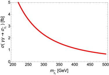
Figure 1: The stoponium production cross section $\sigma(\gamma\gamma\rightarrow\sigma_{\tilde{t}_{1}})$ as a function of the lightest stop mass $m_{\tilde{t}_{1}}$. The center-of-mass energy of the electron beams is taken to be $\sqrt{s_{ee}}=1.26\,m_{\sigma}$, which maximizes the cross section.

In Fig. 1, we plot the stoponium production cross section

$$\sigma(\gamma\gamma\rightarrow\sigma_{\tilde{t}_{1}})=\frac{16\pi^{2}\Gamma(\sigma_{\tilde{t}_{1}}\rightarrow\gamma\gamma)}{m_{\sigma}}\frac{1}{s_{ee}L_{ee}}\int_{z_{0}^{2}/y_{m}}^{y_{m}}\frac{dy}{y}\left[\frac{d^{2}L_{\gamma\gamma}}{dydy^{\prime}}\frac{1\pm\xi_{2}(y)\xi_{2}(y^{\prime})}{2}\right]_{y^{\prime}=z_{0}^{2}/y},$$ (29)

taking $\sqrt{s_{ee}}=1.26\,m_{\sigma}$, which maximizes the cross section. The stoponium production cross section can be as large as $O(1)$ fb for $m_{\tilde{t}_{1}}\lesssim 500\ {\rm GeV}$.

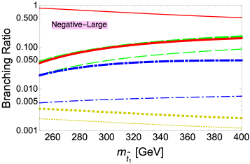
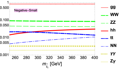
Figure 2: The branching ratios of the stoponium as functions of the lightest stop mass, taking $m_{\tilde{t}_{2}}=4\ {\rm TeV}$, $m_{\chi^{0}_{1}}=m_{\tilde{t}_{1}}-50\,{\rm GeV}$, $\tan\beta=10$, $\mu=2\ {\rm TeV}$ with negative-large (left) and negative-small (right) solutions of the $A_{t}$, which give $m_{h}=125.7\ {\rm GeV}$. In the legend, $NN$ stands for the branching ratio of the decay to the lightest neutralino pair.

In Fig. 2, we show the branching ratios of the stoponium as functions of the lightest stop mass, taking $m_{\tilde{t}_{2}}=4\ {\rm TeV}$, $m_{\chi^{0}_{1}}=m_{\tilde{t}_{1}}-50\,{\rm GeV}$, $\tan\beta=10$, $\mu=2\ {\rm TeV}$ and negative-large or negative-small solutions of the $A_{t}$ parameter. The positive $A_{t}$ solutions give similar branching ratios. The $gg$ decay mode dominates the stoponium decay, and this may be an useful mode for stoponium searches at photon-photon colliders. However, the $gg$ branching ratio is completely determined by the strong coupling constant, and measuring this mode does not give much information on SUSY interactions. Therefore, we do not investigate this mode in this study. Although $WW$ and $ZZ$ decay modes have non-negligible branching ratios of ${\cal O}(1-10)\%$, they suffer from large SM backgrounds [1, 2, 12]. We therefor investigate $hh$ decay mode in the following sections as a probe to the SUSY interactions, especially to the stop sector. We will see in the next section that the signal-to-background ratio of the $\gamma\gamma\rightarrow\sigma_{\tilde{t}_{1}}\rightarrow hh$ process may be large enough to be observed at the ILC-based photon-photon collider.

3 $\sigma_{\tilde{t}_{1}}\rightarrow hh$ search at a photon-photon collider

In this section, we discuss a search strategy for the $hh$ decay mode of the stoponium at the photon-photon collider. We assume an upgraded ILC, whose energy is planned to reach $\sqrt{s_{ee}}=1\rm{TeV}$ [7] with the integrated luminosity of $\mathcal{L}_{ee}\sim 1\,{\rm ab}^{-1}$.

For our numerical calculation, we adopt four sample SUSY model points with $m_{\tilde{t}_{1}}=250$, $300$, $350$, and $400\ {\rm GeV}$ as summarized in Table 1.

	Point 1	Point 2	Point 3	Point 4
$m_{\tilde{t}_{1}}$	250	300	350	400
$m_{\tilde{t}_{2}}$	3480	3810	4110	4080
$A_{t}$	-4370	-4940	-5460	-5670
$m_{\tilde{\chi}_{1}^{0}}$	150	250	300	350
$\sqrt{s_{ee}}$ [GeV]	625	750	875	1000
$\sigma(\gamma\gamma\rightarrow\sigma_{\tilde{t}_{1}}\rightarrow hh)$ [fb]	0.34	0.26	0.2	0.18

Table 1: The sample SUSY models we adopt in our collider analyses. All the SUSY parameters are given in units of GeV. We take $\tan\beta=10$ and $\mu=2$ TeV in all the sample points. Other SUSY particle masses and soft-breaking trilinear couplings are taken to be $2$ TeV. These sample points realize $m_{h}=125.7$ GeV. The employed c.m. energy of the electron beams and the cross section of the $\gamma\gamma\rightarrow\sigma_{\tilde{t}_{1}}\rightarrow hh$ process are also shown for each sample point.

We assume that the lighter stop and the lightest neutralino, $\tilde{\chi}^{0}_{1}$, will be discovered before the photon-photon collider experiment is carried out. In addition, if the stop is within the kinematical reach of the photon-photon collider, detailed studies of the stop will have been already performed with the $e^{+}e^{-}$ collisions at the ILC, and hence we also assume that the basic properties of the lighter stop such as the mass and the chirality will be measured at the ILC before the start of the photon-photon collider. We consider the cases where the bino is the lightest SUSY particle (LSP) with $m_{\tilde{\chi}_{1}^{0}}=150,250,300$, and $350$ GeV for each $m_{\tilde{t}_{1}}$, respectively. Other SUSY particles are assumed to be sufficiently heavy ($\stackrel{{\scriptstyle>}}{{{}_{\sim}}}2$ TeV) and irrelevant to our photon collider study. $\tan\beta$ and $\mu$ parameter are taken to be 10 and 2 TeV, respectively, for all the sample points, and the Higgs mass of 125.7 GeV is realized by adjusting the $A_{t}$ parameter and the heavier stop mass, $m_{\tilde{t}_{2}}$. (For our numerical calculation of the Higgs mass, we use FeynHiggs ​v2.11.3 [13].) In order to maximize the stoponium production cross section, we adjust the c.m. energy of the electron beams as $\sqrt{s_{ee}}\sim 1.26\,m_{\sigma}$ for each sample point shown in Table 1. The cross sections of the process $\gamma\gamma\rightarrow\sigma_{\tilde{t}_{1}}\rightarrow hh$ for those sample points are also shown in the Table.

3.1 Signal event selection

From Table 1 we see that the cross sections $\sigma(\gamma\gamma\rightarrow\sigma_{\tilde{t}_{1}}\rightarrow hh)$ for the sample points are of ${\cal O}$(0.1) fb, and then the process would give only ${\cal O}$(100) events at $1\,{\rm ab}^{-1}$. Therefore, we use the main $b\bar{b}$ decay mode of the Higgs boson for the signal process, i.e., $\gamma\gamma\rightarrow\sigma_{\tilde{t}_{1}}\rightarrow hh\rightarrow b\bar{b}b\bar{b}$.

In order to simulate the signal process, we generate events where a scalar particle (which corresponds to the stoponium) is produced at the photon-photon collider and decayed to a Higgs pair with their subsequent decays to $b\bar{b}$, using MadGraph5_aMC@NLO v2 [14]; the luminosity function of the colliding photons [6, 9] are implemented by modifying the electron PDF routines in MadGraph5. The cross section of the events is normalized to that of the signal process according to Eq. (22). The generated events are then showered with PYTHIA v6.4 [15] and passed to DELPHES v3 [16] for fast detector simulations. In the detector simulation, we assume energy resolutions of 2%/$\sqrt{E\textrm{(GeV)}}\oplus 0.5$% and 50%/$\sqrt{E\textrm{(GeV)}}\oplus 3$% for an electromagnetic calorimeter and hadron calorimeter, respectively, based on ILC TDR [17]. FastJet v3 [18] is employed for jet clustering using the anti-$k_{t}$ algorithm [19] with the distance parameter of 0.5.

From the generated events, we first select events containing more than four jets and satisfying ${p_{T}}>30$ GeV and $|\eta|<2.0$ for all of the four highest $p_{T}$ jets (Preselection), where $p_{T}$ and $\eta$ are the transverse momentum and pseudo-rapidity, respectively. We then impose the following cuts successively:

$${\rm S1}: \,m_{\sigma}-60\,{\rm GeV}\leq M_{\rm{4jets}}\leq m_{\sigma}+40\,{\rm GeV}.$$

$${\rm S2}: \,N_{\rm{b\mathchar 45\relax tag}}\geq 3.$$

$${\rm S3}: \,105.7\,{\rm GeV}\leq M_{1}\leq 130.7\,{\rm GeV},$$

$$\,100.7\,(105.7)\,{\rm GeV}\leq M_{2}\leq 130.7\,{\rm GeV\hskip 10.00002pt(for\,the\,Point\,1\,(2,\,3,\,4))}.$$

$${\rm S4}: \,\min\{\Delta R_{1},\Delta R_{2}\}\leq 1.4,$$

$$\,\max\{\Delta R_{1},\Delta R_{2}\}\leq 1.8.$$

Here $M_{\rm{4jets}}$ is the invariant mass of the four highest $p_{T}$ jets. $N_{\rm{b\mathchar 45\relax tag}}$ is the number of b-tagged jets in each event, where we assume 80% b-tag efficiency, and 10% and 0.1% mis-tag rates for $c$ jets and $u,d,s$ jets, respectively. In S3 and S4, $M_{1(2)}$ and $\Delta R_{1(2)}$ are defined as follows. We first divide the leading four jets into two jet pairs. Among three possible pairings, we choose the one which minimizes $(M_{1}-m_{h})^{2}+(M_{2}-m_{h})^{2}$, where $M_{1}$ and $M_{2}$ are the invariant masses of the jet pairs such that

$$|M_{1}-m_{h}|<|M_{2}-m_{h}|.$$ (30)

$\Delta R_{1(2)}$ is defined as

$$\Delta R_{1(2)}=\sqrt{(\Delta\eta_{1(2)})^{2}+(\Delta\phi_{1(2)})^{2}},$$ (31)

where $\Delta\eta_{1(2)}$ and $\Delta\phi_{1(2)}$ are the differences of pseudo-rapidities and azimuthal angles between the paired jets with the invariant mass of $M_{1(2)}$, respectively.

3.2 Backgrounds

After imposing the selection cuts, the relevant background processes are the non-resonant $hh$, $bb\bar{b}\bar{b}$, $b\bar{b}c\bar{c}$, $cc\bar{c}\bar{c}$, $b\bar{b}q\bar{q}$ (where $q=u,d,s$), $t\bar{t}$, $ZZ$, $W^{+}W^{-}$ and $W^{+}W^{-}Z$ production processes. The event numbers after all the selection cuts are imposed are estimated for the above background processes as in the signal process case, except the non-resonant $hh$ and $ZZ$ backgrounds, which are loop induced processes.

As for $hh$ and $ZZ$ backgrounds, we use approximate estimations; the event numbers of the non-resonant $hh$ background after each cuts are estimated with $\sim$ 15% uncertainty, and the event numbers of the $ZZ$ background are estimated as the upper bounds after all cuts are applied. We will see in Sec. 3.3 that even these rough estimations are enough for our study and leave more detailed estimations for future works.

In the following, we describe our procedure to estimate the non-resonant $hh$ and $ZZ$ backgrounds. The production cross sections of background processes at the photon-photon collider can be expressed in the similar way as for the signal process discussed in Sec. 2.2:

$$\sigma(\gamma\gamma\rightarrow F;s_{ee}) =\frac{1}{L_{ee}}\int_{0}^{y_{m}}dydy^{\prime}\frac{d^{2}L_{\gamma\gamma}}{dydy^{\prime}}\hat{\sigma}(\gamma\gamma\rightarrow F;s_{\gamma\gamma}=yy^{\prime}s_{ee})$$

$$=\sum_{\lambda\lambda^{{}^{\prime}}=++,+-}\int^{y_{m}}_{0}dz\left[\frac{1}{L_{ee}}\frac{dL_{\gamma\gamma}}{dz}\frac{1\pm\xi_{2}\xi^{\prime}_{2}}{2}\right]\!\!\left(z\right)\,\,\hat{\sigma}_{\lambda\lambda^{{}^{\prime}}}(\gamma\gamma\rightarrow F;s_{\gamma\gamma}=z^{2}s_{ee}),$$ (32)

where

$$\left[\frac{1}{L_{ee}}\frac{dL_{\gamma\gamma}}{dz}\frac{1\pm\xi_{2}\xi^{\prime}_{2}}{2}\right]\!\!\left(z\right) \equiv 2z\int^{y_{m}}_{z^{2}/y_{m}}\frac{dy}{y}\frac{1}{L_{ee}}\frac{d^{2}L_{\gamma\gamma}}{dydy^{\prime}}\frac{1\pm\xi_{2}(y)\xi_{2}(y^{\prime})}{2}\Bigl{|}_{y^{\prime}=z^{2}/y},$$ (33)

with $z=\sqrt{s_{\gamma\gamma}/s_{ee}}$. In the second line, contributions from $\xi_{1}$ and $\xi_{3}$ are negligible since we consider axial symmetric electron beams; the sign in front of the stokes parameters are taken to be positive (negative) for $\lambda\lambda^{{}^{\prime}}=++(+-)$.

$\bm{\gamma\gamma\rightarrow hh\rightarrow bb\bar{b}\bar{b}}$

First, let us discuss the non-resonant Higgs pair production process. The dominant background contributions are from Higgs pairs decaying to bottom quarks. Based on Eq. (32), the cross section after all selection cuts are imposed, $\sigma_{\rm cut}(\gamma\gamma\rightarrow hh\rightarrow bb\bar{b}\bar{b};s_{ee})$, is given by

$$\sigma_{\rm cut}(\gamma\gamma\rightarrow hh\rightarrow bb\bar{b}\bar{b}) ={\rm Br}(h\rightarrow b\bar{b})^{2}\sum_{\lambda\lambda^{{}^{\prime}}=++,+-}\int^{y_{m}}_{0}dz\int^{y_{m}}_{z^{2}/y_{m}}dy\,\,\frac{1}{L_{ee}}\frac{d^{2}L_{\gamma\gamma}}{dzdy}\left(\frac{1\pm\xi_{2}\xi^{\prime}_{2}}{2}\right)$$

$$\mspace{30.0mu}\times\int^{1}_{0}d\cos\theta^{*}\frac{d\hat{\sigma}_{\lambda\lambda^{{}^{\prime}}}\left(\gamma\gamma\rightarrow hh;s_{\gamma\gamma}=z^{2}s_{ee},\theta^{*}\right)}{d\cos\theta^{*}}\,\varepsilon_{\lambda\lambda^{{}^{\prime}}}(z,y,\theta^{*}),$$ (34)

where $\varepsilon_{\lambda\lambda^{{}^{\prime}}}(z,y,\theta^{*})$ is the total efficiency of all the selection cuts for events with a c.m. energy $\sqrt{s_{\gamma\gamma}}=z\sqrt{s_{ee}}$, a total energy measured in the laboratory frame $E_{\rm{lab}}=(y+z^{2}/y)E_{ee}$, and Higgs scattering angle $\theta^{*}$ in the c.m. frame of the $\gamma\mathchar 45\relax\gamma$ collision.

We approximate this expression by neglecting the angular dependence of the Higgs production cross section. In Fig. 3, we plot the luminosity-weighted differential cross section

$$\Big{\langle}\frac{d\hat{\sigma}_{\lambda\lambda^{{}^{\prime}}}\left(\gamma\gamma\rightarrow hh,s_{\gamma\gamma},\theta^{*}\right)}{d\cos\theta^{*}}\Big{\rangle} \equiv\frac{d\hat{\sigma}_{\lambda\lambda^{{}^{\prime}}}\left(\gamma\gamma\rightarrow hh;s_{\gamma\gamma},\theta^{*}\right)}{d\cos\theta^{*}}\left[\frac{1}{L_{ee}}\frac{dL_{\gamma\gamma}}{dz}\frac{1\pm\xi_{2}\xi^{\prime}_{2}}{2}\right]\!\!\left(z=\sqrt{s_{\gamma\gamma}/s_{ee}}\right),$$ (35)

for $\sqrt{s_{\gamma\gamma}}=m_{\sigma}$ and $m_{\sigma}-60\,{\rm GeV}$ with $m_{\sigma}=500$ GeV (Point 1).

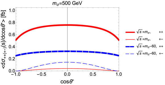
Figure 3: The angular distributions of the luminosity-weighted cross sections evaluated at $\sqrt{s_{\gamma\gamma}}=m_{\sigma}$ (thick lines) and $m_{\sigma}-60$ GeV (thin lines) for $m_{\sigma}=500$ GeV ($\sqrt{s_{ee}}$ = 625 GeV) case. The solid-red and dashed-blue lines represent $(++)$ and $(+-)$ helicity configurations of initial photons, respectively.

In evaluating the differential cross section $d\hat{\sigma}_{\lambda\lambda^{{}^{\prime}}}(\gamma\gamma\rightarrow hh;s_{\gamma\gamma},\theta^{*})/d\cos\theta^{*}$, we use the one-loop expressions given by Ref. [20].

From the figure, we see that the luminosity-weighted differential cross sections for the $(++)$ photon helicity are larger than those for the $(+-)$ photon helicity. Those cross sections do not change significantly over the whole range of $\cos\theta^{*}$ for both $\sqrt{s_{\gamma\gamma}}$ choices. We have also checked that Point 4 shows a similar behavior with $\sqrt{s_{\gamma\gamma}}=800$ GeV. Therefore, we approximate that Higgs pairs are produced almost isotropically in the c.m. frame of the photon collision. Then, Eq. (34) is written as

$$\sigma_{\rm cut}(\gamma\gamma\rightarrow hh\rightarrow bb\bar{b}\bar{b};s_{ee}) \simeq{\rm Br}(h\rightarrow b\bar{b})^{2}$$

$$\times\sum_{\lambda\lambda^{{}^{\prime}}=++,+-}\int_{0}^{y_{m}}dz \left[\frac{1}{L_{ee}}\frac{dL_{\gamma\gamma}}{dz}\left(\frac{1\pm\xi_{2}\xi^{\prime}_{2}}{2}\right)\,\varepsilon_{\lambda\lambda^{{}^{\prime}}}\right]\!\!(z)\,\,\frac{d\hat{\sigma}_{\lambda\lambda^{{}^{\prime}}}(\gamma\gamma\rightarrow hh;s_{\gamma\gamma}=z^{2}s_{ee})}{d\cos\theta^{*}}\Bigg{|}_{\rm ave.},$$ (36)

where

$$\frac{d\hat{\sigma}_{\lambda\lambda^{{}^{\prime}}}(\gamma\gamma\rightarrow hh;s_{\gamma\gamma})}{d\cos\theta^{*}}\Bigg{|}_{\rm ave.} \equiv\int^{1}_{0}d\cos\theta^{*}\,\frac{d\hat{\sigma}_{\lambda\lambda^{{}^{\prime}}}(\gamma\gamma\rightarrow hh;s_{\gamma\gamma},\theta^{*})}{d\cos\theta^{*}},$$ (37)

$$\left[\frac{1}{L_{ee}}\frac{dL_{\gamma\gamma}}{dz}\left(\frac{1\pm\xi_{2}\xi^{\prime}_{2}}{2}\right)\,\varepsilon_{\lambda\lambda^{{}^{\prime}}}\right]\!\!(z)\,\, \equiv\int^{y_{m}}_{z^{2}/y_{m}}dy\int^{1}_{0}d\cos\theta^{*}\frac{1}{L_{ee}}\frac{d^{2}L_{\gamma\gamma}}{dzdy}\left(\frac{1\pm\xi_{2}\xi^{\prime}_{2}}{2}\right)\,\varepsilon_{\lambda\lambda^{{}^{\prime}}}(z,y,\theta^{*}).$$ (38)

Note that we approximate the differential cross section by its averaged value over $\cos\theta^{*}$. The total cut efficiency is estimated by generating event samples of isotropically produced Higgs pairs with the luminosity function, setting the c.m. energy of the Higgs pairs to $\sqrt{s_{\gamma\gamma}}$ and imposing all the selection cuts on the generated events.

Finally, we comment on our approximation that the Higgs pairs are produced isotropically. Using the maximum value of the differential cross section over the $\cos\theta^{*}$ range instead of the averaged one in Eq. (36), we obtain the upper bound of $\sigma_{\rm cut}$. We check that the differences between the upper bounds and our approximated cross section, Eq. (36), are less than 15 %. This can be regarded as the uncertainty of our approximation, which is sufficient for our study as we will see in the next subsection.

$\bm{\gamma\gamma\rightarrow ZZ\rightarrow bb\bar{b}\bar{b},b\bar{b}c\bar{c}}$

Next, we discuss the $ZZ$ background. The dominant background contributions are from $bb\bar{b}\bar{b}$ and $b\bar{b}c\bar{c}$ decay modes. Instead of directly estimating the $ZZ$ background cross section with all the selection cuts being imposed ($\sigma_{\rm cut}$), we set an upper bound on the cross section by removing the Preselection and S4 cuts since estimation of the efficiencies of those cuts needs more detailed simulation. The upper bound is written as

$$\sigma_{\rm cut} (\gamma\gamma\rightarrow ZZ\rightarrow bb\bar{b}\bar{b},b\bar{b}c\bar{c};s_{ee})\stackrel{{\scriptstyle<}}{{{}_{\sim}}}\left\{{\rm Br}(Z\rightarrow b\bar{b})^{2}\varepsilon^{4b}_{\rm S2}+2\,{\rm Br}(Z\rightarrow b\bar{b}){\rm Br}(Z\rightarrow c\bar{c})\varepsilon^{2b2c}_{\rm S2}\right\}\,\varepsilon_{\rm S3}$$

$$\hskip 10.00002pt\times\sum_{\lambda\lambda^{{}^{\prime}}=++,+-}\int^{\sqrt{s_{\rm max}/s_{ee}}}_{\sqrt{s_{\rm min}/s_{ee}}}dz\,\left[\frac{1}{L_{ee}}\frac{dL_{\gamma\gamma}}{dz}\frac{1\pm\xi_{2}\xi^{\prime}_{2}}{2}\right]\!\!\left(z\right)\hat{\sigma}_{\lambda\lambda^{{}^{\prime}}}\left(\gamma\gamma\rightarrow ZZ;s_{\gamma\gamma}=z^{2}s_{ee}\right),$$ (39)

where $\varepsilon^{4b(2b2c)}_{\rm S2}$ and $\varepsilon_{\rm S3}$ are the efficiencies of the S2 cut for the $bb\bar{b}\bar{b}\,(b\bar{b}c\bar{c})$ decay mode and the S3 cut, respectively. In evaluating $\hat{\sigma}_{\lambda\lambda^{{}^{\prime}}}\left(\gamma\gamma\rightarrow ZZ;s_{\gamma\gamma}\right)$, we use the one-loop expressions given in Ref. [12]. In Eq. (39), we approximately take into account the efficiencies of the S1, S2 and S3 cuts as follows. The effect of the S1 cut is approximated by limiting the integration interval, setting the upper and lower limits to those of the S1 cut , i.e., $\sqrt{s}_{\rm max}=m_{\sigma}+40$ GeV and $\sqrt{s}_{\rm min}=m_{\sigma}-60$ GeV for each sample model points. The efficiency of the S2 cut corresponds to the probability that three or four jets are $b$-tagged from the $bb\bar{b}\bar{b}$ ($b\bar{b}c\bar{c}$) final state and is obtained as $\varepsilon^{4b(2b2c)}_{\rm S2}\sim 0.82\,(0.12)$. The S3 cut efficiency is estimated from simulated event samples of $Z$ boson pairs produced in the $e^{+}e^{-}$ collision, setting the c.m. energy of the $Z$ boson pair at $m_{\sigma}$ since the peak region of the photon-photon luminosity is tuned at around this energy. This upper bound on the $ZZ$ background will be used in estimating the upper bound on the total background in the next subsection.

3.3 Results

We present expected signal and background event numbers with all the selection cuts imposed for the sample model points in Table 2.

	Point 1	Point 2	Point 3	Point 4
$m_{\tilde{t}_{1}}$ [ GeV ]	$250$	$300$	$350$	$400$
$\sigma(\gamma\gamma\rightarrow\sigma_{\tilde{t}_{1}}\rightarrow hh)$ [fb]	0.34	0.26	0.2	0.18
signal	$14.2$	$13.5$	$12.5$	$12.4$
total background	$\stackrel{{\scriptstyle<}}{{{}_{\sim}}}$ 3.9	$\stackrel{{\scriptstyle<}}{{{}_{\sim}}}$ 3.2	$\stackrel{{\scriptstyle<}}{{{}_{\sim}}}$ 2.3	$\stackrel{{\scriptstyle<}}{{{}_{\sim}}}$ 2.3
non-resonant $hh$	$2.2$	$2.1$	$1.7$	$1.4$
$bb\bar{b}\bar{b}$	$0.5$	$0.2$	$0.0$	$0.0$
$c\bar{c}b\bar{b}$	$0.4$	$0.5$	$0.2$	$0.1$
$ZZ$	$\stackrel{{\scriptstyle<}}{{{}_{\sim}}}0.8$	$\stackrel{{\scriptstyle<}}{{{}_{\sim}}}0.5$	$\stackrel{{\scriptstyle<}}{{{}_{\sim}}}0.3$	$\stackrel{{\scriptstyle<}}{{{}_{\sim}}}0.7$
$t\bar{t}$	$0.1$	$0.0$	$0.1$	$0.1$
$cc\bar{c}\bar{c}$	$0.0$	$0.0$	$0.0$	$0.0$
$b\bar{b}q\bar{q}$	$0.0$	$0.0$	$0.0$	$0.0$
$W^{+}W^{-}$	$0.0$	$0.0$	$0.0$	$0.0$
$W^{+}W^{-}Z$	$0.0$	$0.0$	$0.0$	$0.0$
Significance $Z_{0}$	$\stackrel{{\scriptstyle>}}{{{}_{\sim}}}5.2$	$\stackrel{{\scriptstyle>}}{{{}_{\sim}}}5.3$	$\stackrel{{\scriptstyle>}}{{{}_{\sim}}}5.5$	$\stackrel{{\scriptstyle>}}{{{}_{\sim}}}5.5$

Table 2: The number of the signal and background events that pass all the selection cuts and the signal significance $Z_{0}$ with $\mathcal{L}_{ee}=1\rm{ab}^{-1}$ for each sample point.

Here, we assume the integrated electron-beam luminosity of $1\mspace{5.0mu}\textrm{ab}^{-1}$. More than ten signal events are expected for all the sample points, while background events are effectively reduced to less than four events. We estimate the expected significance of detecting the $\sigma_{\tilde{t}_{1}}\rightarrow hh$ decay mode using an approximated formula based on the Poisson distribution [21]:

$$Z_{0}=\sqrt{2\left\{(S+B)\ln(1+S/B)-S\right\}},$$ (40)

with $S$ $(B)$ being the expected signal (total background) event number. The significance $Z_{0}$ for each sample point is also presented in Table 2. Because we only estimate the upper bounds on the $ZZ$ background, the expected significances are regarded as lower bounds. We see that in order for the $5\sigma$ detection, the signal cross sections, $\sigma(\gamma\gamma\rightarrow\sigma_{\tilde{t}_{1}}\rightarrow hh)$, of $0.34-0.18$ fb are required for the stoponium masses of 500 – 800 GeV, respectively. In the rest of this section, we discuss how background events are reduced by imposing the selection cuts.

After imposing all the selection cuts, the major background source is the non-resonant Higgs pair ($hh$) production process, and the contributions from other background sources except $bb\bar{b}\bar{b}$, $b\bar{b}c\bar{c}$ and $ZZ$ are negligibly small. We present the cut-flow information along with the cut efficiencies in parentheses for the sample Point 1 in Table 3 and for other points in Table 4, where only the non-negligible background processes are presented.

Point 1	Preselection $+$ S1	$+$ S2	$+$ S3	$+$ S4
signal	$32.8$	$26.8$ $(0.82)$	$18.0$ $(0.67)$	$14.2$ $(0.79)$
non-resonant $hh$	$4.9$	$4.0$ $(0.82)$	$2.8$ $(0.70)$	$2.2$ $(0.76)$
$bb\bar{b}\bar{b}$	$42$	$34$ $(0.82)$	$1.9$ $(0.05)$	$0.5$ $(0.25)$
$c\bar{c}b\bar{b}$	$540$	$67$ $(0.12)$	$2.1$ $(0.03)$	$0.4$ $(0.17)$
$ZZ$	-	-	-	$\stackrel{{\scriptstyle<}}{{{}_{\sim}}}0.8$
$t\bar{t}$	$39$	$2.2$ $(0.06)$	$0.1$ $(0.04)$	$0.1$ $(1.00)$
$cc\bar{c}\bar{c}$	$1160$	$4.3$ $(0.004)$	$0.2$ $(0.04)$	$0.0$ $(0.17)$
$b\bar{b}q\bar{q}$	$1190$	$1.5$ $(0.001)$	$0.1$ $(0.04)$	$0.0$ $(0.25)$
$W^{+}W^{-}$	$195800$	$3.9$ $(2\times 10^{-5})$	$0.0$ $(0.00)$	$0.0$ $(0.00)$
$W^{+}W^{-}Z$	$5.0$	$0.2$ $(0.04)$	$0.0$ $(0.02)$	$0.0$ $(1.00)$

Table 3: The number of the signal and background events after the successive application of the cuts with $\mathcal{L}_{ee}=1\rm{ab}^{-1}$ for the sample Point 1. The efficiencies of each selection cuts are also presented in the parentheses. For the $ZZ$ background, only an upper bound on the number of events that pass all the cuts is presented.

Point 2	Preselection $+$ S1	$+$ S2	$+$ S3	$+$ S4
signal	$28.6$	$23.4$ $(0.82)$	$14.6$ $(0.62)$	$13.5$ $(0.92)$
non-resonant $hh$	$4.1$	$3.4$ $(0.82)$	$2.3$ $(0.67)$	$2.1$ $(0.93)$
$bb\bar{b}\bar{b}$	$30$	$25$ $(0.82)$	$0.3$ $(0.01)$	$0.2$ $(0.54)$
$c\bar{c}b\bar{b}$	$390$	$49$ $(0.12)$	$1.1$ $(0.02)$	$0.5$ $(0.43)$
Point 3	Preselection $+$ S1	$+$ S2	$+$ S3	$+$ S4
signal	$23.2$	$19.0$ $(0.82)$	$12.9$ $(0.68)$	$12.5$ $(0.97)$
non-resonant $hh$	$3.1$	$2.5$ $(0.82)$	$1.8$ $(0.70)$	$1.7$ $(0.97)$
$bb\bar{b}\bar{b}$	$24$	$19$ $(0.82)$	$0.1$ $(0.01)$	$0.0$ $(0.00)$
$c\bar{c}b\bar{b}$	$300$	$37$ $(0.12)$	$0.3$ $(0.01)$	$0.2$ $(0.50)$
Point 4	Preselection $+$ S1	$+$ S2	$+$ S3	$+$ S4
signal	$21.6$	$17.7$ $(0.82)$	$12.6$ $(0.71)$	$12.4$ $(0.99)$
non-resonant $hh$	$2.4$	$2.0$ $(0.82)$	$1.4$ $(0.71)$	$1.4$ $(0.99)$
$bb\bar{b}\bar{b}$	$17$	$14$ $(0.82)$	$0.1$ $(0.01)$	$0.0$ $(0.00)$
$c\bar{c}b\bar{b}$	$230$	$28$ $(0.12)$	$0.3$ $(0.01)$	$0.1$ $(0.50)$

Table 4: Same as Table 3 but for the sample Point 2, 3 and 4, and only the non-negligible background processes are shown.

The selection cut S2, which requires three or four jets are b-tagged, then plays an important role in reducing the large portion of the background events which needs some non-$b$ jets to be mistagged to pass the cut.

The selection cut S3, relevant to the di-jet invariant masses, also reduce most of the background events efficiently, except for non-resonant $hh$, by imposing Higgs mass constraints on two pairs of jets. At this stage, only the non-resonant $hh$, $bb\bar{b}\bar{b}$, $c\bar{c}b\bar{b}$ and $ZZ$ backgrounds remains sizable.

The selection cut S4, which is based on $\Delta R$ distributions, further reduces the remained $bb\bar{b}\bar{b}$ and $c\bar{c}b\bar{b}$ backgrounds. In Figs. 4, we present the $\min\{\Delta R_{1},\Delta R_{2}\}$ and $\max\{\Delta R_{1},\Delta R_{2}\}$ distributions of signal and $bb\bar{b}\bar{b}$ plus $c\bar{c}b\bar{b}$ background after imposing the Preselection, S1, S2 and S3 cuts for the sample Point 1.

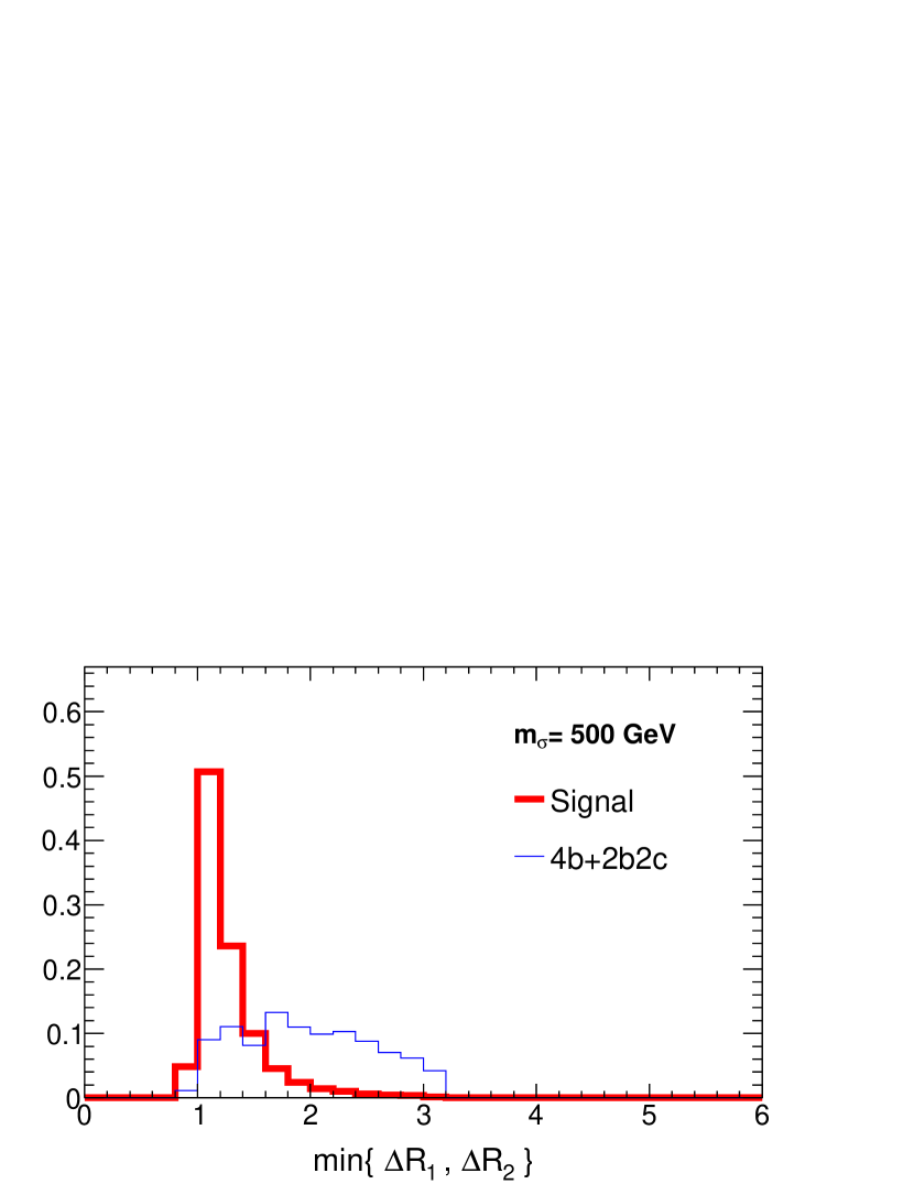
(a) $\min\{\Delta R_{1},\Delta R_{2}\}$

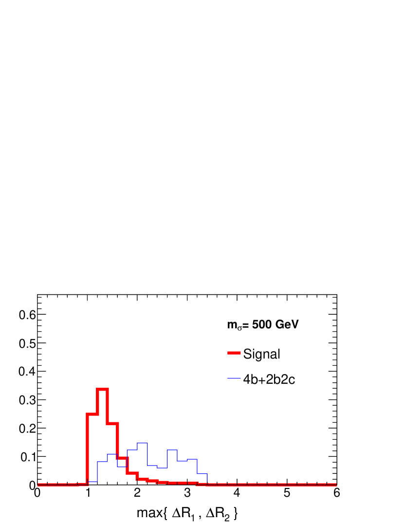
(b) $\max\{\Delta R_{1},\Delta R_{2}\}$

Figure 4: The normalized distributions of $\min\{\Delta R_{1},\Delta R_{2}\}$ (left) and $\max\{\Delta R_{1},\Delta R_{2}\}$ (right) for the Point 1 with all the cuts except S4 being imposed. The thick red lines are for the signal and the thin blue lines for the $bb\bar{b}\bar{b}$ plus $c\bar{c}b\bar{b}$.

We see that $\Delta R$ tends to be small for the signal, while it can be large up to $\sim 3$ for the $bb\bar{b}\bar{b}$ plus $b\bar{b}c\bar{c}$ backgrounds. This difference makes the S4 cut efficient for reducing those backgrounds, and can be understood qualitatively as follows. The di-jet systems from the non-resonant multi-jet processes tend to distribute in the large $|\eta|$ region more than the di-jet systems from decays of rather isotropically produced Higgs bosons. In general, two jets in a di-jet system with larger $|\eta|$ tend to have larger azimuthal angle difference, $\Delta\phi$, and thus larger $\Delta R$; this mainly makes the difference in the $\Delta R$ distributions between the signal and the four-jet backgrounds above.

4 Implication to the stop sector

In the previous section, we have shown that there are possibilities to detect the di-Higgs decay mode of the stoponium and measure its cross section, $\sigma(\gamma\gamma\rightarrow\sigma_{\tilde{t}_{1}}\rightarrow hh)$. In this section we discuss its implication for extracting information on the SUSY parameters in the stop sector: $m_{\tilde{t}_{2}}$ and $A_{t}$. Since we assume that the lighter stop and the lightest neutralino are discovered by the time when the photon-photon collider experiment will be carried out, their masses are regarded as known parameters. Some other SUSY parameters may also be known by that time, but we just assume them as unknown parameters for a conservative approach.

The heavier stop mass, $m_{\tilde{t}_{2}}$, and stop trilinear coupling, $A_{t}$, may be determined from the constraints of the measured cross section and Higgs mass up to the four-fold solutions when we fix the other SUSY parameters. This is illustrated in Fig. 5, where the four solutions appear on the $m_{\tilde{t}_{2}}$–$A_{t}$ plane as the intersections between the contours of the stoponium cross section and Higgs mass.

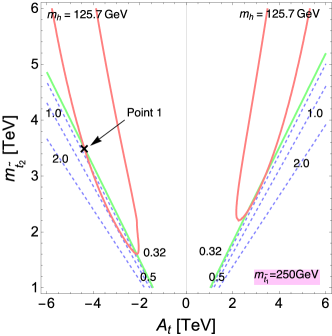
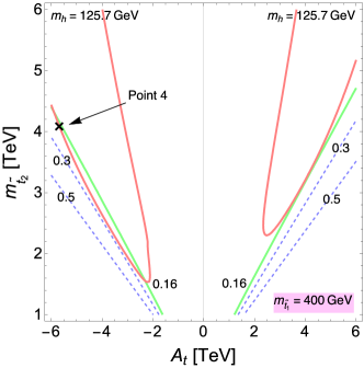
Figure 5: The contours of the stoponium cross section, $\sigma(\gamma\gamma\rightarrow\sigma_{\tilde{t}_{1}}\rightarrow hh)$, and $m_{h}=125.7$ GeV on the $m_{\tilde{t}_{2}}$–$A_{t}$ plane for $m_{\tilde{t}_{1}}=250\ {\rm GeV}$ (left) and 400 GeV (right). We take $m_{\tilde{\chi}^{0}_{1}}=150$ GeV (left) and 350 GeV (right), $\tan\beta=10$, $\mu=2\ {\rm TeV}$ and other SUSY parameters having dimension of mass equal to 2 TeV, except the trilinear couplings of the first and second generation sfermions which are set to zero. The dashed-blue lines show the cross sections, while the solid-green line represents the cross section which allows $5\sigma$ detection of the $\sigma_{\tilde{t}_{1}}\rightarrow hh$ mode. The contour labels are given in units of fb. The red curve shows the Higgs boson mass constraint. The sample model points in Sec. 3 are shown with the cross symbol.

Since we assume that the true SUSY parameter values are not known (except $m_{\tilde{t}_{1}}$ and $m_{\chi^{0}_{1}}$), we scan over the unknown SUSY parameters relevant to the stoponium cross sections and Higgs mass, finding possible solutions of $m_{\tilde{t}_{2}}$ and $A_{t}$ in the parameter space. As an example result, we discuss upper bounds on $m_{\tilde{t}_{2}}$ and $|A_{t}|$. For the paramter scan, we employ the phenomenological MSSM [22] as a SUSY framework. Besides $\tan\beta$ and $\mu$ parameters, which are relevant to the stoponium cross section and Higgs mass at tree level, the parameter space is spanned by the mass parameters of sbottom, stau and gluino: $M_{\tilde{b}_{R}},M_{\tilde{\tau}_{L}},M_{\tilde{\tau}_{R}}$ and $M_{3}$. For simplicity, we set $M_{\tilde{\tau}_{L}}=M_{\tilde{\tau}_{R}}$ and fix all the other SUSY mass parameters and trilinear couplings to 2 TeV. We check that the bounds are insensitive to these assumptions. In Table 5, we summarize the scanned and assumed SUSY parameters for each $m_{\tilde{t}_{1}}$.

$m_{\tilde{t}_{1}}$ [GeV]	250	300	350	400
$m_{\tilde{\chi}^{0}_{1}}$ [GeV]	150	250	300	350
$\sigma(\gamma\gamma\rightarrow\sigma_{\tilde{t}_{1}}\rightarrow hh)$ [fb]	0.34	0.26	0.2	0.18
$\tan\beta$	[10, 60] (3 points)
$\mu$	[-10, 10] TeV (6 points)
$M_{3}$	[2, 10] TeV (3 points)
$M_{\tilde{b}_{R}}$	[2, 10] TeV (3 points)
$M_{\tilde{\tau}_{L}}=M_{\tilde{\tau}_{R}}$	[2, 10] TeV (3 points)
$M_{{\rm others}}$	2 TeV
$A_{b}=A_{\tau}$	2 TeV
$A_{{\rm 1st}/{\rm 2nd}}$	2 TeV

Table 5: The assumed SUSY parameter values and the ranges of the scanned parameters. The parentheses show the number of points taken for the corresponding parameter. The stoponium cross sections are set such that they allow $5\sigma$ detection of the $\gamma\gamma\rightarrow\sigma_{\tilde{t}_{1}}\rightarrow hh$ process. $M_{\rm others}$ represents the SUSY mass parameters which are not explicitly shown in the Table. $A_{{\rm 1st}/{\rm 2nd}}$ denotes the trilinear couplings related to the first and second generation sfermions.

We assume that the $\gamma\gamma\rightarrow\sigma_{\tilde{t}_{1}}\rightarrow hh$ process will be measured with more than $5\sigma$ significance and regard the cross sections given in Table 2 as the measured ones for each $m_{\tilde{t}_{1}}$. In obtaining bounds, we take into account statistical uncertainties of the signal measurements.

As shown in Table 6, the obtained upper bounds on $m_{\tilde{t}_{2}}$ and $|A_{t}|$ are $3.8-4.7$ TeV and $5.1-6.5$ TeV, respectively.

$m_{\tilde{t}_{1}}$ [GeV]	250	300	350	400
$m_{\tilde{t}_{2}}^{\rm upper}$ [TeV]	3.8	4.2	4.6	4.7
$|A_{t}|^{\rm upper}$ [TeV]	5.1	5.7	6.2	6.5

Table 6: The obtained upper bounds on $m_{\tilde{t}_{2}}$ and $|A_{t}|$ by the parameter scan for each $m_{\tilde{t}_{1}}$ value.

The upper bounds on $m_{\tilde{t}_{2}}$ are obtained well within the scanned parameter space and do not change significantly even if we extend the parameter space to $|\mu|,M_{3},M_{\tilde{b}_{R}},M_{\tilde{\tau}}<14$ TeV from 10 TeV. On the other hand, the upper bounds on $|A_{t}|$ increase non-negligibly as we extend the parameter space; the dominant effects on the $|A_{t}|$ bounds are from the change of the $\mu$ parameter range since the $A_{t}$ parameter linearly depends on the $\mu$ parameter through $A_{t}=X_{t}-\mu\cot\beta$. Thus, information on the $\mu$ parameter is important to obtain stringent bounds on $A_{t}$. As illustrated in this section, detection of the di-Higgs decay mode of the stoponium and measurement of its cross section would provide useful information on the stop sector.

5 Summary and conclusion

In this study, we have investigated the detectability of the stoponium in the di-Higgs decay mode at the photon-photon collider. We have assumed that the lightest neutralino is the LSP, and the lighter stop is the next-to-lightest SUSY particle (NLSP). We have also assumed that those particles would be discovered before the photon-photon collider experiment will be carried out and that the basic properties of the stop such as the mass and left-right mixing angle could be studied by that time. We have concentrated on the scenario where the mass difference between the stop and the neutralino is small enough, and the stop can form the stoponium.

The detectability of the stoponium di-Higgs decays has been investigated by estimating the stoponium signal and standard model backgrounds and optimizing the signal selection cuts. It has been found that $5\sigma$ detection of the di-Higgs decay mode is possible with the integrated electron-beam luminosity of 1 ${\rm ab}^{-1}$ if the signal cross section, $\sigma(\gamma\gamma\rightarrow\sigma_{\tilde{t}_{1}}\rightarrow hh)$, of 0.34, 0.26, 0.2 and 0.18 fb are realized for the stoponium masses of 500, 600, 700 and 800 GeV, respectively. As concrete examples, we have provided the four sample model points in MSSM, corresponding to those stoponium masses and realizing such cross sections.

Finally, we have discussed the implication of the cross section measurement of the stoponium di-Higgs decay mode for the MSSM stop sector. Combining the measured cross section with the Higgs-mass constraint, we have shown that there would be the upper bound on the heavier stop mass for each lighter stop and lightest neutralino masses. $A_{t}$ parameter would also be constrained, depending on other SUSY parameters such as $\mu$ and $\tan\beta$. In conclusion, there are possibilities that the di-Higgs decay mode of the stoponium would be observed unambiguously at the future photon-photon collider and provide new insights into the stop sector.

Acknowledgments: The work is supported by Grant-in-Aid for Scientific research Nos. 23104008 and 26400239.

Appendix A Photon luminosity function

We use the luminosity function of the following form [5, 6, 9]:

$$\frac{1}{L_{ee}}\frac{d^{2}L_{\gamma\gamma}}{dydy^{\prime}}=f(x,y)B(x,y)f(x,y^{\prime})B(x,y^{\prime}).$$ (41)

The function $f$ is given by

$$f(x,y)=\frac{2\pi\alpha_{e}^{2}}{\sigma_{c}xm_{e}^{2}}C_{00}(x,y),$$ (42)

where the function $C_{00}$ is given in Eq. (24), and

$$\sigma_{c}=\sigma_{c}^{\rm(np)}+\lambda_{e}P_{l}\sigma_{1},$$ (43)

with

$$\sigma_{c}^{\rm(np)} =\frac{2\pi\alpha_{e}^{2}}{xm^{2}_{e}}\left[\left(1-\frac{4}{x}-\frac{8}{x^{2}}\right)\ln(x+1)+\frac{1}{2}+\frac{8}{x}-\frac{1}{2(x+1)^{2}}\right],$$ (44)

$$\sigma_{1} =\frac{2\pi\alpha_{e}^{2}}{xm^{2}_{e}}\left[\left(1+\frac{2}{x}\right)\ln(x+1)-\frac{5}{2}+\frac{1}{x+1}-\frac{1}{2(x+1)^{2}}\right].$$ (45)

The function $B$ is given by

$$B(x,y)=\left\{\begin{array}[]{ll}\displaystyle{\exp\left[-\frac{\rho^{2}}{8}\left(\frac{x}{y}-x-1\right)\right]}&~{}:~{}y_{m}/2<y<y_{m}\\ 0&~{}:~{}\mbox{otherwise}\end{array}\right.,$$ (48)

with $y_{m}=x/(x+1)$. In our numerical calculation, we take $\rho=1$ [9].

Appendix B Matrix elements

We summarize the matrix elements for the stop anti-stop annihilation processes used in our study [10, 11]. We assume that all the SUSY particles, except the stops, sbottoms and lightest neutralino, are sufficiently heavy, and neglect their contributions. We also assume that the lightest neutralino is purely bino-like. In the following expressions, the summations over the color indices of the initial stop and anti-stop have been implicitly performed as

$$\left|\mathcal{M}\left(\tilde{t}_{1}\tilde{t}^{*}_{1}\rightarrow AB\right)\right|^{2}=\left|\frac{1}{3}\sum_{a}\mathcal{M}\left(\tilde{t}_{1}^{a}\,\tilde{t}_{1}^{a*}\rightarrow AB\right)\right|^{2},$$ (49)

and the explicit color summations should be taken for the final-state colored paricles.

(1) $\bm{gg}$

In the $v=0$ limit (where $v$ is the velocity of the stops in the initial state), the contributions from the $t$- and $u$-channel stop exchanges are absent. Therefore, the squared matrix element dose not depend on the MSSM parameters and is given by

$$\sum_{\rm{color,\,helicity}}\left|\mathcal{M}\left(\tilde{t}_{1}\tilde{t}^{*}_{1}\rightarrow gg\right)\right|^{2}_{v=0}=\left(\frac{16\pi}{3}\alpha_{s}\right)^{2}.$$ (50)

(2) $\bm{\gamma\gamma}$

As in the $gg$ final-state case, the squared matrix element for the $\gamma\gamma$ final state dose not depend on the MSSM parameters and is given by

$$\sum_{\rm{helicity}}\left|\mathcal{M}\left(\tilde{t}_{1}\tilde{t}^{*}_{1}\rightarrow\gamma\gamma\right)\right|^{2}_{v=0}=128\pi^{2}\left(\frac{2}{3}\right)^{4}\alpha^{2}_{e}.$$ (51)

(3) $\bm{hh}$

The squared matrix element is given by

$$\left|\mathcal{M}\left(\tilde{t}_{1}\tilde{t}^{*}_{1}\rightarrow hh\right)\right|^{2}_{v=0}=\Biggl{\{}\frac{2\left(c^{(2)}_{\tilde{t}_{1}}\right)^{2}}{2m^{2}_{\tilde{t}_{1}}-m^{2}_{h}} +\frac{2\left(c^{(2)}_{\tilde{t}_{1}\tilde{t}_{2}}\right)^{2}}{m^{2}_{\tilde{t}_{1}}+m^{2}_{\tilde{t}_{2}}-m^{2}_{h}}+c^{22}_{11}$$

$$+\frac{c^{(2)}_{\tilde{t}_{1}}}{4m^{2}_{\tilde{t}_{1}}-m^{2}_{h}}\frac{3g\,m_{Z}}{2c_{W}}\cos 2\alpha\sin\left(\beta+\alpha\right)\Biggr{\}}^{2},$$ (52)

where $g$ is the $SU(2)_{L}$ gauge coupling constant, $c_{\rm W}=\cos\theta_{\rm W}$, $s_{\rm W}=\sin\theta_{\rm W}$, and $\alpha$ is the mixing angle of the CP-even Higgs bosons. In addition, $c^{(2)}_{\tilde{t}_{1}}$, $c^{(2)}_{\tilde{t}_{1}\tilde{t}_{2}}$ and $c^{22}_{11}$ are the coefficients of the $\tilde{t}_{1}\tilde{t}_{1}^{*}h$,  $\tilde{t}_{1}\tilde{t}_{2}^{*}h$, and $\tilde{t}_{1}\tilde{t}_{1}^{*}hh$ vertices, respectively, and are given by

$$c^{(2)}_{\tilde{t}_{1}} =\frac{g\,m_{Z}}{c_{W}}\sin\left(\alpha+\beta\right)\left(\frac{1}{2}\cos^{2}\theta_{\tilde{t}}-\frac{2}{3}s^{2}_{W}\cos 2\theta_{\tilde{t}}\right)-\frac{g\,m^{2}_{t}}{m_{W}}\frac{\cos\alpha}{\sin\beta}$$

$$\mspace{294.0mu}+\frac{g\,m_{t}}{2m_{W}\sin\beta}\sin 2\theta_{\tilde{t}}\left(A_{t}\cos\alpha-\mu\sin\alpha\right),$$ (53)

$$c^{(2)}_{\tilde{t}_{1}\tilde{t}_{2}} =\frac{g\,m_{Z}}{c_{W}}\sin(\alpha+\beta)\sin 2\theta_{\tilde{t}}\left(\frac{2}{3}s_{W}^{2}-\frac{1}{4}\right)+\frac{g\,m_{t}}{2m_{W}\sin\beta}\cos 2\theta_{\tilde{t}}\left(A_{t}\cos\alpha-\mu\sin\alpha\right),$$ (54)

$$c^{22}_{11}\,\, =\frac{g^{2}}{2}\left[\frac{\cos 2\alpha}{c_{W}^{2}}\left(\frac{1}{2}\cos^{2}\theta_{\tilde{t}}-\frac{2}{3}s^{2}_{W}\cos 2\theta_{\tilde{t}}\right)-\frac{m_{t}^{2}}{m_{W}^{2}}\frac{\cos^{2}\alpha}{\sin^{2}\beta}\right].$$ (55)

(4) $\bm{W^{+}W^{-}}$

The squared matrix element is given by

$$\sum_{\rm{spin}}\left|\mathcal{M}\left(\tilde{t}_{1}\tilde{t}^{*}_{1}\rightarrow W^{+}W^{-}\right)\right|^{2}_{v=0}=2\left(a^{T}_{WW}\right)^{2}+\left(a^{L}_{WW}\right)^{2},$$ (56)

where $a^{T}_{WW}$ and $a^{L}_{WW}$ correspond to the transverse and longitudinal components of the matrix element and are given by

$$a^{T}_{WW}=\mathcal{M}^{+1+1}=\mathcal{M}^{-1-1}=-\left(\frac{g^{2}}{2}\cos^{2}\theta_{\tilde{t}}-\frac{g_{hWW}c^{(2)}_{\tilde{t}_{1}}}{4m^{2}_{\tilde{t}_{1}}-m^{2}_{h}}\right),$$ (57)

and

$$a^{L}_{WW}=\mathcal{M}^{00}=\left(\frac{2m^{2}_{\tilde{t}_{1}}}{m_{W}^{2}}-1\right) \left(\frac{g^{2}}{2}\cos^{2}\theta_{\tilde{t}}-\frac{g_{hWW}c^{(2)}_{\tilde{t}_{1}}}{4m^{2}_{\tilde{t}_{1}}-m^{2}_{h}}\right)$$

$$-2\left(\frac{m^{2}_{\tilde{t}_{1}}}{m_{W}^{2}}-1\right)\left(\frac{g^{2}\cos^{2}\theta_{\tilde{t}}\,m_{\tilde{t}_{1}}^{2}}{m_{\tilde{t}_{1}}^{2}+m_{\tilde{b}_{L}}^{2}-m_{W}^{2}}\right),$$ (58)

respectively. Here, $m_{\tilde{b}_{L}}$ is the left-handed sbottom mass (where we neglect the left-right sbottom mixing), and $g_{hWW}$ is the coefficient of the $hW^{+}W^{-}$ vertex, which is given by

$$g_{hWW}=g\,m_{W}\sin\left(\beta-\alpha\right).$$ (59)

Note that in the $v\rightarrow 0$ limit, the contribution of the $s$-channel $Z$ boson exchange is absent.

(5) $\bm{ZZ}$

The squared matrix element is given by

$$\sum_{\rm{spin}}\left|\mathcal{M}\left(\tilde{t}_{1}\tilde{t}^{*}_{1}\rightarrow ZZ\right)\right|^{2}_{v=0}=2\left(a^{T}_{ZZ}\right)^{2}+\left(a^{L}_{ZZ}\right)^{2},$$ (60)

where

$$a^{T}_{ZZ}=\mathcal{M}^{+1+1}=\mathcal{M}^{-1-1}=\frac{1}{c_{W}^{2}}\left[2g^{2}\left\{\left(\frac{1}{4}-\frac{2}{3}s_{W}^{2}\right)\cos^{2}\theta_{\tilde{t}}+\frac{4}{9}s^{4}_{W}\right\}-\frac{g_{hWW}c^{(2)}_{\tilde{t}_{1}}}{4m^{2}_{\tilde{t}_{1}}-m^{2}_{h}}\right],$$ (61)

and

$$a^{L}_{ZZ}=\mathcal{M}^{00}=-\frac{1}{c_{W}^{2}}\left(\frac{2m^{2}_{\tilde{t}_{1}}}{m_{Z}^{2}}-1\right)\left[2g^{2}\left\{\left(\frac{1}{4}-\frac{2}{3}s_{W}^{2}\right)\cos^{2}\theta_{\tilde{t}}+\frac{4}{9}s_{W}^{4}\right\}-\frac{g_{hWW}c^{(2)}_{\tilde{t}_{1}}}{4m^{2}_{\tilde{t}_{1}}-m^{2}_{h}}\right]$$

$$\mspace{20.0mu}+\frac{2g^{2}m^{2}_{\tilde{t}_{1}}}{c_{W}^{2}}\left(\frac{m^{2}_{\tilde{t}_{1}}}{m_{Z}^{2}}-1\right)\left[\frac{\left(\cos^{2}\theta_{\tilde{t}}-\frac{4}{3}s^{2}_{W}\right)^{2}}{2m^{2}_{\tilde{t}_{1}}-m^{2}_{Z}}+\frac{\cos^{2}\theta_{\tilde{t}}\sin^{2}\theta_{\tilde{t}}}{m^{2}_{\tilde{t}_{1}}+m^{2}_{\tilde{t}_{2}}-m^{2}_{Z}}\right]$$ . (62)

(6) $\bm{Z\gamma}$

The squared matrix element is given by

$$\sum_{{\rm spin,\,helicity}}\left|\mathcal{M}\left(\tilde{t}_{1}\tilde{t}^{*}_{1}\rightarrow Z\gamma\right)\right|^{2}_{v=0}=8\left(\frac{2}{3}\right)^{2}g^{2}g^{\prime 2}\left(\frac{1}{2}\cos^{2}\theta_{\tilde{t}}-\frac{2}{3}s_{W}^{2}\right)^{2},$$ (63)

where $g^{{}^{\prime}}$ is the hypercharge gauge coupling constant.

(7) $\bm{b\bar{b}}$

The squared matrix element is given by

$$\sum_{\rm{color,\,spin}}\left|\mathcal{M}\left(\tilde{t}_{1}\tilde{t}^{*}_{1}\rightarrow b\bar{b}\right)\right|^{2}_{v=0}=24\left(m^{2}_{\tilde{t}_{1}}-m^{2}_{b}\right)\left(\frac{g\,m_{b}}{2m_{W}}\frac{\sin\alpha}{\cos\beta}\frac{c^{(2)}_{\tilde{t}_{1}}}{4m^{2}_{\tilde{t}_{1}}-m^{2}_{h}}\right)^{2}.$$ (64)

(8) $\bm{t\bar{t}}$

The squared matrix element is given by

$$\sum_{{\rm color,\,spin}} \left|\mathcal{M}\left(\tilde{t}_{1}\tilde{t}^{*}_{1}\rightarrow t\bar{t}\right)\right|^{2}_{v=0}=24\left(m^{2}_{\tilde{t}_{1}}-m^{2}_{t}\right)$$

$$\times \left\{\frac{1}{3}\frac{m_{\tilde{\chi}^{0}_{1}}\left(a_{1}^{2}-b^{2}_{1}\right)+m_{t}\left(a_{1}^{2}+b^{2}_{1}\right)}{m_{t}^{2}-m_{\tilde{t}_{1}}^{2}-m_{\tilde{\chi}^{0}_{1}}^{2}}-\frac{g\,m_{t}}{2m_{W}}\frac{\cos\alpha}{\sin\beta}\frac{c^{(2)}_{\tilde{t}_{1}}}{4m^{2}_{\tilde{t}_{1}}-m^{2}_{h}}\right\}^{2},$$ (65)

where

$$a_{1}=-\frac{1}{\sqrt{2}}g^{\prime}\left(\frac{1}{6}\cos\theta_{\tilde{t}}-\frac{2}{3}\sin\theta_{\tilde{t}}\right),$$ (66)

$$b_{1}=-\frac{1}{\sqrt{2}}g^{\prime}\left(\frac{1}{6}\cos\theta_{\tilde{t}}+\frac{2}{3}\sin\theta_{\tilde{t}}\right).$$ (67)

(9) $\bm{\tilde{\chi}^{0}_{1}\tilde{\chi}^{0}_{1}}$

The squared matrix element is given by

$$\sum_{{\rm spin}}\left|\mathcal{M}\left(\tilde{t}_{1}\tilde{t}^{*}_{1}\rightarrow\tilde{\chi}^{0}_{1}\tilde{\chi}^{0}_{1}\right)\right|^{2}_{v=0}=8\left(m^{2}_{\tilde{t}_{1}}-m^{2}_{\tilde{\chi}^{0}_{1}}\right)\left\{\frac{2m_{t}\left(a_{1}^{2}-b_{1}^{2}\right)+2m_{\tilde{\chi}^{0}_{1}}\left(a_{1}^{2}-b_{1}^{2}\right)}{m_{\tilde{\chi}^{0}_{1}}^{2}-m^{2}_{\tilde{t}_{1}}-m_{t}^{2}}\right\}^{2}.$$ (68)

References

- [1] D. S. Gorbunov and V. A. Ilyin, JHEP 0011, 011 (2000) [hep-ph/0004092].
- [2] D. S. Gorbunov, V. A. Ilyin and V. I. Telnov, Nucl. Instrum. Meth. A 472, 171 (2001) [hep-ph/0012175].
- [3] M. J. Herrero, A. Mendez and T. G. Rizzo, Phys. Lett. B 200, 205 (1988); V. D. Barger and W. Y. Keung, Phys. Lett. B 211, 355 (1988); H. Inazawa and T. Morii, Phys. Rev. Lett. 70, 2992 (1993); M. Drees and M. M. Nojiri, Phys. Rev. D 49, 4595 (1994); M. Drees and M. M. Nojiri, Phys. Rev. Lett. 72, 2324 (1994); M. Antonelli and N. Fabiano, Eur. Phys. J. C 16, 361 (2000); S. P. Martin, Phys. Rev. D 77, 075002 (2008); S. P. Martin and J. E. Younkin, Phys. Rev. D 80, 035026 (2009); Y. Kats and M. D. Schwartz, JHEP 1004, 016 (2010); J. E. Younkin and S. P. Martin, Phys. Rev. D 81, 055006 (2010); D. Kahawala and Y. Kats, JHEP 1109, 099 (2011); V. Barger, M. Ishida and W.-Y. Keung, Phys. Rev. Lett. 108, 081804 (2012); Y. Kats and M. J. Strassler, JHEP 1211, 097 (2012); C. Kim, A. Idilbi, T. Mehen and Y. W. Yoon, Phys. Rev. D 89, no. 7, 075010 (2014); N. Kumar and S. P. Martin, Phys. Rev. D 90, no. 5, 055007 (2014); B. Batell and S. Jung, JHEP 1507, 061 (2015).
- [4] B. Grzadkowski and J. F. Gunion, Phys. Lett. B 294 (1992) 361 D. L. Borden, D. A. Bauer and D. O. Caldwell, Phys. Rev. D 48 (1993) 4018; M. Kramer, J. H. Kuhn, M. L. Stong and P. M. Zerwas, Z. Phys. C 64 (1994) 21; J. F. Gunion and J. G. Kelly, Phys. Lett. B 333 (1994) 110; H. Anlauf, W. Bernreuther and A. Brandenburg, Phys. Rev. D 52 (1995) 3803 [Phys. Rev. D 53 (1996) 1725]; G. J. Gounaris and G. P. Tsirigoti, Phys. Rev. D 56 (1997) 3030 [Phys. Rev. D 58 (1998) 059901]; T. Ohgaki, T. Takahashi and I. Watanabe, Phys. Rev. D 56 (1997) 1723; I. Watanabe et al., KEK-REPORT-97-17, AJC-HEP-31, HUPD-9807, ITP-SU-98-01, DPSU-98-4; G. Japaridze and A. Tkabladze, Phys. Lett. B 433 (1998) 139; A. T. Banin, I. F. Ginzburg and I. P. Ivanov, Phys. Rev. D 59 (1999) 115001; M. Melles, W. J. Stirling and V. A. Khoze, Phys. Rev. D 61 (2000) 054015; S. Y. Choi and J. S. Lee, Phys. Rev. D 62 (2000) 036005; E. Asakawa, J. i. Kamoshita, A. Sugamoto and I. Watanabe, Eur. Phys. J. C 14 (2000) 335; E. Asakawa, S. Y. Choi, K. Hagiwara and J. S. Lee, Phys. Rev. D 62 (2000) 115005; D. M. Asner, J. B. Gronberg and J. F. Gunion, Phys. Rev. D 67 (2003) 035009; S. Bae, B. Chung and P. Ko, Eur. Phys. J. C 54 (2008) 601; P. Niezurawski, A. F. Zarnecki and M. Krawczyk, JHEP 0211 (2002) 034; P. Niezurawski, A. F. Zarnecki and M. Krawczyk, Acta Phys. Polon. B 34 (2003) 177; R. M. Godbole, S. D. Rindani and R. K. Singh, Phys. Rev. D 67 (2003) 095009 [Phys. Rev. D 71 (2005) 039902]; E. Asakawa and K. Hagiwara, Eur. Phys. J. C 31 (2003) 351; P. Niezurawski, A. F. Zarnecki and M. Krawczyk, Acta Phys. Polon. B 36 (2005) 833; K. Monig and A. Rosca, Eur. Phys. J. C 57 (2008) 535; N. Bernal, D. Lopez-Val and J. Sola, Phys. Lett. B 677 (2009) 39; L. Wang, F. Xu and J. M. Yang, JHEP 1001 (2010) 107; E. Asakawa, D. Harada, S. Kanemura, Y. Okada and K. Tsumura, Phys. Rev. D 82 (2010) 115002; D. Lopez-Val and J. Sola, Phys. Lett. B 702 (2011) 246; X. G. He, S. F. Li and H. H. Lin, Mod. Phys. Lett. A 28 (2013) 1350085; D. M. Asner et al., arXiv:1310.0763 [hep-ph]; H. Ito, T. Moroi and Y. Takaesu, arXiv:1601.01144 [hep-ph]; A. Djouadi, J. Ellis, R. Godbole and J. Quevillon, arXiv:1601.03696 [hep-ph].
- [5] I. F. Ginzburg, G. L. Kotkin, V. G. Serbo and V. I. Telnov, Nucl. Instrum. Meth. 205, 47 (1983).
- [6] I. F. Ginzburg, G. L. Kotkin, S. L. Panfil, V. G. Serbo and V. I. Telnov, Nucl. Instrum. Meth. A 219, 5 (1984).
- [7] T. Behnke et al., [arXiv:1306.6327 [physics.acc-ph]].
- [8] K. Hagiwara, K. Kato, A. D. Martin and C. K. Ng, Nucl. Phys. B 344, 1 (1990).
- [9] I. F. Ginzburg and G. L. Kotkin, Eur. Phys. J. C 13, 295 (2000) [hep-ph/9905462].
- [10] M. Drees and M. M. Nojiri, Phys. Rev. D 49, 4595 (1994); [hep-ph/9312213].
- [11] S. P. Martin, Phys. Rev. D 77, 075002 (2008); [arXiv:0801.0237 [hep-ph]].
- [12] G. J. Gounaris, J. Layssac, P. I. Porfyriadis and F. M. Renard, Eur. Phys. J. C 13, 79 (2000) [hep-ph/9909243].
- [13] S. Heinemeyer, W. Hollik and G. Weiglein, Comput. Phys. Commun. 124 (2000) 76; S. Heinemeyer, W. Hollik and G. Weiglein, Eur. Phys. J. C 9 (1999) 343; G. Degrassi, S. Heinemeyer, W. Hollik, P. Slavich and G. Weiglein, Eur. Phys. J. C 28 (2003) 133; M. Frank, T. Hahn, S. Heinemeyer, W. Hollik, H. Rzehak and G. Weiglein, JHEP 0702 (2007) 047; T. Hahn, S. Heinemeyer, W. Hollik, H. Rzehak and G. Weiglein, Phys. Rev. Lett. 112 (2014) 14, 141801.
- [14] J. Alwall, R. Frederix, S. Frixione, V. Hirschi, F. Maltoni, O. Mattelaer, H.-S. Shao and T. Stelzer et al., JHEP 1407, 079 (2014) [arXiv:1405.0301 [hep-ph]].
- [15] T. Sjostrand, S. Mrenna and P. Z. Skands, JHEP 0605, 026 (2006) [hep-ph/0603175].
- [16] J. de Favereau et al. [DELPHES 3 Collaboration], JHEP 1402, 057 (2014) [arXiv:1307.6346 [hep-ex]].
- [17] T. Behnke, J. E. Brau, P. N. Burrows, J. Fuster, M. Peskin, M. Stanitzki, Y. Sugimoto and S. Yamada et al., [arXiv:1306.6329 [physics.ins-det]].
- [18] M. Cacciari, G. P. Salam and G. Soyez, Eur. Phys. J. C 72 (2012) 1896; M. Cacciari and G. P. Salam, Phys. Lett. B 641 (2006) 57
- [19] M. Cacciari, G. P. Salam and G. Soyez, JHEP 0804, 063 (2008) [arXiv:0802.1189 [hep-ph]].
- [20] G. V. Jikia, Nucl. Phys. B 412, 57 (1994).
- [21] G. Cowan, K. Cranmer, E. Gross and O. Vitells, Eur. Phys. J. C 71, 1554 (2011) [Eur. Phys. J. C 73, 2501 (2013)] [arXiv:1007.1727 [physics.data-an]].
- [22] C. F. Berger, J. S. Gainer, J. L. Hewett and T. G. Rizzo, JHEP 0902, 023 (2009) [arXiv:0812.0980 [hep-ph]].