Maximum leave-one-out likelihood estimation for location parameter of unbounded densities

Abstract: Maximum likelihood estimation of a location parameter fails when the density have unbounded mode. An alternative approach is considered by leaving out a data point to avoid the unbounded density in the full likelihood. This modification give rise to the leave-one-out likelihood. We propose an ECM algorithm which maximises the leave-one-out likelihood. It was shown that the estimator which maximises the leave-one-out likelihood is consistent and super-efficient. However, other asymptotic properties such as the optimal rate of convergence and asymptotic distribution is still under question. We use simulations to investigate these asymptotic properties of the location estimator using our proposed algorithm.

Keywords: unbounded likelihood, variance gamma distribution, ECM algorithm, asymptotic distribution.

1 Introduction

Asymptotic properties of maximum likelihood estimators for location parameters are well known for the case when the likelihood is bounded and even non-differentiable (Rao,, 1968), but the methodology breaks down when the likelihood is unbounded at certain points. Alternate approaches for the unbounded case have been considered in Ibragimov and Khasminskii, 1981a ; Ibragimov and Khasminskii, 1981b and in Rao, (1966) where they proved consistency results using the Bayesian approach.

Under the likelihood approach however, modifications to the full likelihood is necessary. A possible solution is to leave out a data point closest to the location parameter in the full likelihood which might cause the density to become unbounded. This modification leads to a concept known as the leave-one-out (LOO) likelihood proposed by Podgórski and Wallin, (2015). They proved consistency and super-efficiency of the location estimator that maximises the LOO likelihood. More precisely, they have found a lower bound for the rate of convergence of the location estimator. However, other asymptotic properties such as optimal rate of convergence and the asymptotic distribution are yet to be proven.

Our main objective of the paper is to propose an expectation/conditional maximisation (ECM) algorithm (Meng and Rubin,, 1993) to obtain the maximum LOO estimator of parameters from variance gamma (VG) distribution (Madan and Seneta,, 1990). This proposed algorithm is an extension to the EM algorithm for estimating the location parameter of symmetric generalised Laplace distribution in Podgórski and Wallin, (2015). Additionally, they have not yet supplied simulations results using their algorithm. The convergence properties of the ECM algorithm for the LOO likelihood is similar to the ECM algorithm for the full likelihood. Our other objective is to analyse the asymptotic behaviour of the maximum LOO likelihood estimator for the location parameter, by applying our proposed algorithm to simulated data from a VG distribution with different samples sizes and shape parameters.

There are two important reasons why we consider parameter estimation from VG distribution. Firstly, it is part of a more general class of distributions called generalised hyperbolic (GH) distribution where it has a normal mean-variance mixture representation (Barndorff-Nielsen et al.,, 1982). Not only that, it is an important special case that corresponds to the unbounded case of the GH distribution. In order for the GH distribution to approach the VG distribution, it needs to have one of its shape parameters approach the boundary of the parameter space. So the regular EM algorithm that estimates parameters from GH distribution proposed by Protassov, (2004) does not truly capture the unbounded density. Secondly, it has applications in many areas such as financial data, signal processing and quality control. See Kotz et al., (2001) for other applications and further details on generalised Laplace distribution which are fundamentally equivalent to VG distribution.

It is worth emphasising that not only can this methodology deal with estimation of location parameter of unbounded densities, but can deal with other extreme cases where the parameter estimate approaches the boundary of the parameter space, potentially causing the density to become unbounded. One particular example is based on the singularity problem in finite mixture of normals model (Seo and Kim,, 2012).

In summary, Section 2 summarises some important properties of the multivariate skewed VG distribution. Section 3 formulates the maximum LOO likelihood framework for location parameter estimation of distributions with unbounded densities. Section 4 introduces the ECM algorithm using the LOO likelihood to estimate parameters from the multivariate skewed VG distribution. Section 5 presents the simulation study to analyse the asymptotic behaviour of the maximum LOO likelihood estimator for location parameter of the VG distribution. We conclude the paper with further remarks in Section 6.

2 Variance gamma distribution

We will first discuss some important properties of the multivariate skewed VG (MSVG) distribution. The probability density function (pdf) of a $d$-dimensional MSVG distribution is given by

$$f_{VG}(\bm{y})= \frac{2^{1-\frac{d}{2}}\nu^{\nu}}{\left|\bm{\Sigma}\right|^{\frac{1}{2}}\pi^{\frac{d}{2}}\Gamma(\nu)}\frac{K_{\nu-\frac{d}{2}}\left(\sqrt{[2\nu+\bm{\gamma}^{\prime}\bm{\Sigma}^{-1}\bm{\gamma}](\bm{y}-\bm{\mu})^{\prime}\bm{\Sigma}^{-1}(\bm{y}-\bm{\mu})}\right)\exp\left((\bm{y}-\bm{\mu})^{\prime}\bm{\Sigma}^{-1}\bm{\gamma}\right)}{(2\nu+\bm{\gamma}^{\prime}\bm{\Sigma}^{-1}\bm{\gamma})^{\frac{1}{4}(2\nu-d)}[(\bm{y}-\bm{\mu})^{\prime}\bm{\Sigma}^{-1}(\bm{y}-\bm{\mu})]^{\frac{1}{4}(d-2\nu)}}$$ (1)

where $\bm{\mu}\in\mathbb{R}^{d}$ is the location parameter, $\bm{\Sigma}$ is a $d\times d$ positive definite symmetric scale matrix, $\bm{\gamma}\in\mathbb{R}^{d}$ is the skewness parameter, $\nu>0$ is the shape parameter, $\Gamma(\cdot)$ is the gamma function and $K_{\eta}(\cdot)$ is the modified Bessel function of the second kind with index $\eta$ (Gradshteyn and Ryzhik,, 2007, §9.6).

The MSVG distribution has a normal mean-variance mixtures representation given by

$$\bm{y}_{i}|\lambda_{i}\sim\mathcal{N}_{d}(\bm{\mu}+\bm{\gamma}\lambda_{i},\lambda_{i}\bm{\Sigma}),\quad\lambda_{i}\sim\mathcal{G}(\nu,\nu)$$ (2)

where $\mathcal{G}(\alpha,\beta)$ is a Gamma distribution with shape parameters $\alpha>0$, rate parameter $\beta>0$ and pdf

$$f_{G}(\lambda)=\frac{\beta^{\alpha}}{\Gamma(\alpha)}\lambda^{\alpha-1}\exp(-\beta\lambda),\text{ for }\lambda>0.$$

The mean and covariance matrix of a MSVG random vector $\bm{Y}_{i}$ are given by

$$\mathbb{E}(\bm{Y}_{i})=\bm{\mu}+\bm{\gamma}\quad\text{and}\quad\mathbb{C}\mbox{ov}(\bm{Y}_{i})=\bm{\Sigma}+\tfrac{1}{\nu}\bm{\gamma}\bm{\gamma}^{\prime},$$

respectively. The pdf in (1) as $\bm{y}_{i}\rightarrow\bm{\mu}$ is given by

$$f_{VG}(\bm{y}_{i})\sim\begin{cases}\displaystyle 2^{\nu-d}\pi^{-\frac{d}{2}}\left|\bm{\Sigma}\right|^{-\frac{1}{2}}\frac{\Gamma\left(\nu-\tfrac{d}{2}\right)}{\Gamma\left(\nu\right)}\frac{\nu^{\nu}}{(2\nu+\bm{\gamma}^{\prime}\bm{\Sigma}^{-1}\bm{\gamma})^{\frac{2\nu-d}{2}}}&\text{ if }\nu>\tfrac{d}{2},\\ \vspace{2mm}\displaystyle-2^{1-d}\pi^{-\frac{d}{2}}\left|\bm{\Sigma}\right|^{-\frac{1}{2}}\frac{d^{\frac{d}{2}}}{\Gamma\left(\tfrac{d}{2}\right)}\log\left(z_{i}\right)&\text{ if }\nu=\tfrac{d}{2},\\ \vspace{2mm}\displaystyle 2^{-\nu}\pi^{-\frac{d}{2}}\left|\bm{\Sigma}\right|^{-\frac{1}{2}}\frac{\Gamma\left(\tfrac{d}{2}-\nu\right)}{\Gamma\left(\nu\right)}\nu^{\nu}z_{i}^{2\nu-d}&\text{ if }\nu<\tfrac{d}{2},\end{cases}$$ (3)

where

$$z^{2}_{i}=(\bm{y}_{i}-\bm{\mu})^{\prime}\bm{\Sigma}^{-1}(\bm{y}_{i}-\bm{\mu}).$$ (4)

So the density becomes unbounded for the case when $\nu\leq\frac{d}{2}$. This poses some technical difficulty when working with the MSVG distribution as it is unclear whether the shape parameter will fall into the unbounded range.

This problem is illustrated in Figure 1, we first generate ten standardised VG samples with $\nu=0.2$ using the normal mean-variance mixture representation. Then we plot both the full log-likelihood along with the leave-one-out (LOO) log-likelihood with respect to the location parameter. We see that leaving the data point out essentially smooths out the unbounded points of the log-likelihood so the maximum can be well defined. Additionally, if we zoom in at around $\mu=0$, observe that cusps tend to occur between data points.

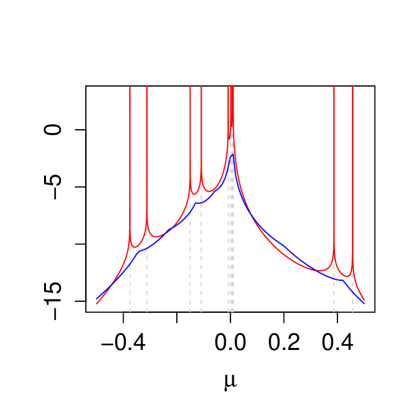
(a) log-likelihood comparison

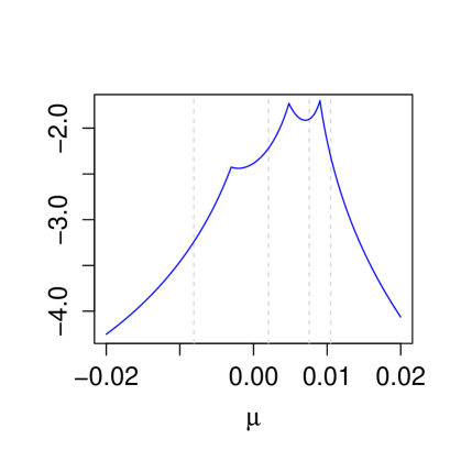
(b) close-up on the LOO log-likelihood

Figure 1: Left: Comparing full log-likelihood (red) vs. LOO log-likelihood (blue) of simulated data from standardised VG distribution with $\nu=0.2$ and sample size of ten (vertical grey dashed lines). Right: Close-up of the left figure at around $\mu=0$ focusing on the LOO log-likelihood.

3 Maximum leave-one-out likelihood

Let us suppose $\bm{y}=(\bm{y}_{1},\cdots,\bm{y}_{n})$ be observed data from MSVG distribution with corresponding missing parameters $\bm{\lambda}=(\lambda_{1},\cdots,\lambda_{n})$, and $\bm{\theta}=(\bm{\mu},\bm{\Sigma},\bm{\gamma},\nu)$ be parameters from MSVG distribution in parameter space $\bm{\Theta}$. The density of the MSVG distribution is unbounded at $\bm{\mu}$ when $\nu\leq\frac{d}{2}$. So the maximum likelihood estimate is not well defined since there are multiple unbounded points in the likelihood function. Thus the Fisher information matrix with respect to $\bm{\mu}$ is also not well defined. Instead we consider the incomplete Fisher information matrix defined by

$$\mathcal{I}_{\epsilon}(\bm{\theta})=\mathbb{E}\left[\left.\left(\frac{\partial}{\partial\theta}\log f(X|\theta)\right)^{2}\right|\left|X\right|>\epsilon\right]$$ (5)

for $\epsilon>0$.

We aim to provide a methodology to estimate parameters from MSVG distribution even with the presence of unboundedness. Although in general this methodology can also apply to distributions which satisfies the following assumptions (Podgórski and Wallin,, 2015):

(A1) $f(x)=p(x)|x|^{\alpha}$, $\alpha\in(-1,0)$, $p$ has bounded derivative on $\mathbb{R}\backslash\{0\}$ and, for some $\epsilon>0$, $f$ is non-zero and continuous either on $[-\epsilon,0]$ or on $[0,\epsilon]$.

(A2) There exist $b>0$ such that $f(x)=O(|x|^{-b-1})$ when $|x|\rightarrow\infty$.

(A3) For all $\epsilon>0$, the incomplete Fisher information is finite.

3.1 Leave-one-out likelihood

Let the observed LOO likelihood is defined as

$$L^{\rm LOO}(\bm{\theta};\bm{y})=\prod_{i\neq k(\bm{\mu})}f(\bm{y}_{i})$$ (6)

where we define the LOO index

$$k(\bm{\mu})=\underset{k\in\{1,\text{...},n\}}{\text{argmin}}(\bm{y}_{k}-\bm{\mu})^{T}\bm{\Sigma}^{-1}(\bm{y}_{k}-\bm{\mu}).$$ (7)

For the case where there are more than one indices, we choose the smallest index. Let the observed LOO log-likelihood be defined as $\ell^{\rm LOO}(\bm{\theta};\bm{y})=\log L^{\rm LOO}(\bm{\theta};\bm{y})$.

Let us define the maximum leave-one-out likelihood estimator denoted as $\hat{\bm{\theta}}^{\rm MLLE}_{n}$ (or simply $\hat{\bm{\theta}}_{n}$) to be the estimator that maximises the LOO likelihood with respect to $\bm{\theta}$. Some main properties of the location estimator $\hat{\mu}_{n}$ is consistency and super-efficient rate of convergence. These properties follow from the main theorem established by Podgórski and Wallin, (2015).

Theorem.

Let $f$ satisfies the assumptions (A1) to (A3) and let $\hat{\mu}_{n}$ be the maximiser of $L^{\rm LOO}(\mu;\bm{y})$. Then $\hat{\mu}_{n}$ is consistent estimator of $\mu$ and for any $\beta<1/(1+\alpha)$,

$$\underset{n\rightarrow\infty}{\lim}n^{\beta}(\hat{\mu}_{n}-\mu)\overset{p}{=}0.$$ (8)

By the main theorem, the lower bound of the rate of convergence for the maximum LOO likelihood location estimator is attained, but doesn’t state the optimal rate of convergence. By setting $\beta=1/(1+\alpha)$, this possibly gives us the optimal rate of convergence. For comparison purposes, we will call this the proposed optimal rate. Additionally, $n^{\beta_{0}}(\hat{\mu}_{n}-\mu)$ will converge to some asymptotic distribution for some suitable choice of $\beta_{0}$. We will investigate the asymptotic properties later in Section 5 using simulations from VG distribution.

4 ECM algorithm for LOO likelihood

Finding the maximum LOO likelihood estimator $\hat{\bm{\theta}}_{n}$ can be difficult as the LOO likelihood has many cusps when $\nu\leq d$, and the LOO index $k(\bm{\mu})$ makes derivatives tedious to work with since the summation and the differential can’t simply be interchanged. Alternatively, we can maximise the complete-data LOO likelihood which allows the implementation of the ECM algorithm.

Using the normal mean-variance mixture representation in Section 2, we can represent the complete-data LOO log-likelihood as

$$\ell^{\rm LOO}(\bm{\theta};\bm{y},\bm{\lambda})= \ell^{\rm LOO}_{N}(\bm{\mu},\bm{\Sigma},\bm{\gamma};\bm{y},\bm{\lambda})+\ell^{\rm LOO}_{G}(\nu;\bm{\lambda})$$ (9)

where the LOO log-likelihood of the conditional normal distribution is given by

$$\ell^{\rm LOO}_{N}(\bm{\mu},\bm{\Sigma},\bm{\gamma};\bm{y},\bm{\lambda})$$

$$=-\frac{n-1}{2}\log|\bm{\Sigma}|-\frac{1}{2}\sum_{i\neq k(\bm{\mu})}\frac{1}{\lambda_{i}}(\bm{y}_{i}-\bm{\mu}-\lambda_{i}\bm{\gamma})^{\prime}\bm{\Sigma}^{-1}(\bm{y}_{i}-\bm{\mu}-\lambda_{i}\bm{\gamma})-\frac{(n-1)d}{2}\log\pi$$ (10)

and the LOO log-likelihood of the conditional gamma distribution is given by

$$\ell^{\rm LOO}_{G}(\nu;\bm{\lambda})=(n-1)(\nu\log\nu-\log\Gamma(\nu))+(\nu-1)\sum_{i\neq k(\bm{\mu})}\log\lambda_{i}-\nu\sum_{i\neq k(\bm{\mu})}\lambda_{i}.$$ (11)

The outline of the ECM algorithm of MSVG distribution using the full likelihood is given in Nitithumbundit and Chan, (2015). However, modifications to the algorithm is necessary when using the LOO likelihood. We will discuss the necessary modifications needed in order to attain local and global convergence of the algorithm.

4.1 E-step

By analysing the conditional posterior distribution of $\lambda_{i}$ given $\bm{y}_{i}$ which has density

$$f(\lambda_{i}|\bm{y}_{i},\bm{\theta})\propto \ \lambda_{i}^{\nu-\frac{d}{2}-1}\exp\left[-\frac{1}{2\lambda_{i}}(\bm{y}_{i}-\bm{\mu})^{\prime}\bm{\Sigma}^{-1}(\bm{y}_{i}-\bm{\mu})-\frac{\lambda_{i}}{2}\left(2\nu+\bm{\gamma}^{\prime}\bm{\Sigma}^{-1}\bm{\gamma}\right)\right]$$ (12)

which corresponds to the pdf of a generalised inverse Gaussian distribution (Embrechts,, 1983), we can calculate the following conditional expectations:

$$\widehat{\lambda_{i}}= \ \mathbb{E}\left(\lambda_{i}|\bm{y},\bm{\theta}\right)=\frac{z_{i}K_{\nu-\frac{d}{2}+1}\left(\sqrt{2\nu+\bm{\gamma}^{\prime}\bm{\Sigma}^{-1}\bm{\gamma}}z_{i}\right)}{\sqrt{2\nu+\bm{\gamma}^{\prime}\bm{\Sigma}^{-1}\bm{\gamma}}K_{\nu-\frac{d}{2}}\left(\sqrt{2\nu+\bm{\gamma}^{\prime}\bm{\Sigma}^{-1}\bm{\gamma}}z_{i}\right)},$$ (13)

$$\widehat{1/\lambda_{i}}= \ \mathbb{E}\left(\frac{1}{\lambda_{i}}\Bigg{|}\bm{y},\bm{\theta}\right)=\frac{\sqrt{2\nu+\bm{\gamma}^{\prime}\bm{\Sigma}^{-1}\bm{\gamma}}K_{\nu-\frac{d}{2}-1}\left(\sqrt{2\nu+\bm{\gamma}^{\prime}\bm{\Sigma}^{-1}\bm{\gamma}}z_{i}\right)}{z_{i}K_{\nu-\frac{d}{2}}\left(\sqrt{2\nu+\bm{\gamma}^{\prime}\bm{\Sigma}^{-1}\bm{\gamma}}z_{i}\right)},$$ (14)

$$\widehat{\log\lambda_{i}}= \ \mathbb{E}\left(\log\lambda_{i}|\bm{y},\bm{\theta}\right)=\log\left(\frac{z_{i}}{\sqrt{2\nu+\bm{\gamma}^{\prime}\bm{\Sigma}^{-1}\bm{\gamma}}}\right)+\frac{K_{\nu-\frac{d}{2}}^{(1,0)}(\sqrt{2\nu+\bm{\gamma}^{\prime}\bm{\Sigma}^{-1}\bm{\gamma}}z_{i})}{K_{\nu-\frac{d}{2}}(\sqrt{2\nu+\bm{\gamma}^{\prime}\bm{\Sigma}^{-1}\bm{\gamma}}z_{i})}$$ (15)

where $\displaystyle K_{\nu}^{(1,0)}(z)=\tfrac{\partial}{\partial\alpha}K_{\alpha}(z)\big{|}_{\alpha=\nu}$ which is approximated using the second-order central difference approximation

$$K_{\nu}^{(1,0)}(z)\approx\frac{K_{\nu+h}(z)-K_{\nu-h}(z)}{2h}$$ (16)

where we let $h=10^{-5}$.

4.2 Derivative of LOO log-likelihood

Derivatives of $\ell^{\rm LOO}_{N}$ with respect to $(\bm{\Sigma},\bm{\gamma})$ are straight forward to calculate using matrix differentiation. Here we will show some difficulties with the derivative with respect to $\bm{\mu}$. The first-order derivative of the complete-data LOO log-likelihood with respect to $\bm{\mu}$ is

$$\frac{\partial}{\partial\bm{\mu}}\ell^{\rm LOO}_{N}=-\frac{1}{2}\left(\frac{\partial}{\partial\bm{\mu}}\sum_{i\neq k(\bm{\mu})}\frac{1}{\lambda_{i}}(\bm{y}_{i}-\bm{\mu}-\lambda_{i}\bm{\gamma})^{\prime}\bm{\Sigma}^{-1}(\bm{y}_{i}-\bm{\mu}-\lambda_{i}\bm{\gamma})\right).$$ (17)

The problem is that the summation index depends on $\bm{\mu}$, so the differential and the summation cannot simply be interchanged. Thus the CM-step for $\bm{\mu}$ does not have a closed form solution.

Alternatively, we can approximate the derivative by simply considering the summation index to be fixed. At the $t$-th iteration, suppose we have $\bm{\mu}^{(t)}$ as our current estimate for $\bm{\mu}$. We can fix the summation index so that we leave out the data point closest to $\bm{\mu}^{(t)}$ instead of $\bm{\mu}$. This gives us an approximation to the derivative

$$\frac{\partial}{\partial\bm{\mu}}\ell^{\rm LOO}_{N} \approx-\frac{1}{2}\left(\frac{\partial}{\partial\bm{\mu}}\sum_{i\neq k(\bm{\mu}^{(t)})}\frac{1}{\lambda_{i}}(\bm{y}_{i}-\bm{\mu}-\lambda_{i}\bm{\gamma})^{\prime}\bm{\Sigma}^{-1}(\bm{y}_{i}-\bm{\mu}-\lambda_{i}\bm{\gamma})\right)$$ (18)

$$=\bm{\Sigma}^{-1}\sum_{i\neq k(\bm{\mu}^{(t)})}\frac{1}{\lambda_{i}}\left(\bm{y}_{i}-\bm{\mu}-\lambda_{i}\bm{\gamma}\right).$$ (19)

Similarly, applying the approximate derivative to $\ell^{\rm LOO}_{N}$ and $\ell^{\rm LOO}_{G}$ with respect to other parameters and solving the approximate derivatives at zero gives us the following CM-steps.

4.3 CM-step

CM-step for $\bm{\mu},\bm{\Sigma},\bm{\gamma}$:

Suppose that the current iterate is $\bm{\theta}^{(t)}$ and $\bm{\lambda}$ is given. After equating each component of the approximate partial derivatives of $\ell^{\rm LOO}_{N}(\bm{\mu},\bm{\Sigma},\bm{\gamma}|\nu,\bm{y},\bm{\lambda})$ to zero, we obtain the following estimates:

$$\bm{\mu}^{(t+1)}= \ \frac{S_{\bm{y}/\lambda}S_{\lambda}-(n-1)S_{\bm{y}}}{S_{1/\lambda}S_{\lambda}-(n-1)^{2}},$$ (20)

$$\bm{\gamma}^{(t+1)}= \ \frac{S_{\bm{y}}-(n-1)\bm{\mu}^{(t+1)}}{S_{\lambda}},$$ (21)

$$\bm{\Sigma}^{(t+1)}= \ \frac{1}{n-1}\sum_{i\neq k(\bm{\mu}^{(t)})}\frac{1}{\lambda_{i}}(\bm{y}_{i}-\bm{\mu}^{(t+1)})(\bm{y}_{i}-\bm{\mu}^{(t+1)})^{\prime}-\frac{1}{n-1}\bm{\gamma}^{(t+1)}\left(\bm{\gamma}^{(t+1)}\right)^{\prime}S_{\lambda},$$ (22)

where the complete data sufficient statistics are:

$$S_{\bm{y}}=\sum_{i\neq k(\bm{\mu}^{(t)})}\bm{y}_{i},\quad S_{\bm{y}/\lambda}=\sum_{i\neq k(\bm{\mu}^{(t)})}\frac{1}{\lambda_{i}}\bm{y}_{i},\quad S_{\lambda}=\sum_{i\neq k(\bm{\mu}^{(t)})}\lambda_{i},\quad S_{1/\lambda}=\sum_{i\neq k(\bm{\mu}^{(t)})}\frac{1}{\lambda_{i}}.$$ (23)

But these estimates won’t guarantee the monotonic convergence of the LOO log-likelihood, since we used the approximate derivatives. However, we can apply a line search to guarantee the monotonic convergence of the ECM algorithm. See Section 4.5 for more details about the lines search.

CM-step for $\nu$:
Given the mixing parameters $\bm{\lambda}$, the estimate $\nu^{(t+1)}$ can be obtained by numerically maximising $\ell^{\rm LOO}_{G}(\nu|\bm{\lambda})$ in (11) with respect to $\nu$ using Newton-Raphson (NR) algorithm where the approximate derivatives is given by:

$$\frac{\partial}{\partial\nu}\ell^{\rm LOO}_{G} =\ (n-1)\left(1+\log\nu-\psi(\nu)\right)+S_{\log\lambda}-S_{\lambda},$$ (24)

$$\frac{\partial^{2}}{\partial\nu^{2}}\ell^{\rm LOO}_{G} =\ (n-1)\left(\frac{1}{\nu}-\psi^{\prime}(\nu)\right)$$ (25)

where $\psi(x)=\frac{d}{dx}\log\Gamma(x)$ is the digamma function and

$$S_{\log\lambda}=\sum_{i\neq k(\bm{\mu}^{(t)})}\log\lambda_{i}.$$ (26)

4.4 Local point search

Even when the LOO likelihood smooths out the unbounded points from the full likelihood, there still exist cusps in the LOO likelihood. So we cannot completely rely on derivative based methods to find the global maximum of LOO likelihood with respect to the location parameter. Nevertheless, these cusp in the LOO likelihood typically occur between data points as seen in Figure 1(b). So for simplicity, we search for data points around the current iterate $\hat{\bm{\mu}}^{(t)}$ and choose the one that increases the LOO likelihood.

Local point search algorithm: Let $(\bm{\mu}^{(t)},\bm{\Sigma}^{(t)},\bm{\gamma}^{(t)},\nu^{(t)})$ be our current location estimates:

(i) Calculate the Mahalanobis distance between $\bm{y}_{i}$ and $\hat{\bm{\mu}}^{(t)}$

$$(\bm{y}_{i}-\hat{\bm{\mu}}^{(t)})^{T}(\bm{\Sigma}^{(t)})^{-1}(\bm{y}_{i}-\hat{\bm{\mu}}^{(t)})$$ (27)

and choose the least $m$ with corresponding data points $\bm{y}_{i_{1}},...,\bm{y}_{i_{m}}$. We choose $m=20$ for our simulation study. Additionally, let $\bm{y}_{i_{0}}=\hat{\bm{\mu}}^{(t)}$ for notational convenience.

(ii) Update the location estimate by choosing $\bm{\mu}$ out of $\{\bm{y}_{i_{0}},\text{...},\bm{y}_{i_{m}}\}$ such that it maximises the LOO log-likelihood

$$\underset{\bm{\mu}\in\{\bm{y}_{i_{0}},\text{...},\bm{y}_{i_{m}}\}}{\text{argmax}}\ell^{\rm LOO}\left(\bm{\mu},\bm{\Sigma}^{(t)},\bm{\gamma}^{(t)},\nu^{(t)};\bm{y}\right).$$ (28)

4.5 Line search

Using the approximate derivatives for the CM-steps does not necessarily increase the LOO log-likelihood. So we need to implement a line search to guarantee the monotonic convergence of the ECM algorithm after each CM-step. Here we abuse the notation by representing $\bm{\theta}^{(t)}$ as the current estimate and $\bm{\theta}^{(t+1)}$ as the updated estimate after the CM-step in Section 4.3.

Let us construct the line search by defining

$$\bm{\theta}^{*}=\bm{\theta}^{(t)}+\alpha\left(\bm{\theta}^{(t+1)}-\bm{\theta}^{(t)}\right)$$ (29)

where $\alpha\in I\subset\mathbb{R}$ and the interval $I$ is chosen so that $\bm{\theta}^{*}\in\bm{\Theta}$. For simplicity, we consider the interval $I=[0,1]$.

Using the optimise function in R, find $\alpha$ such that it maximises the LOO log-likelihood

$$\alpha^{*}=\underset{\alpha\in I}{\text{argmax}}\ell^{\rm LOO}(\bm{\theta}^{*}).$$ (30)

Although finding the maximum of a non-smooth likelihood function is difficult, so alternatively we can choose $\alpha^{*}$ such that

$$\ell^{\rm LOO}(\bm{\theta}^{*};\bm{y})\geq\ell^{\rm LOO}(\bm{\theta}^{(t)};\bm{y}).$$ (31)

4.6 ECM algorithm

Combining the steps we introduced earlier gives us the ECM algorithm for MSVG distribution using the LOO likelihood:

Initialisation step: Choose suitable starting values $(\bm{\mu}_{0},\bm{\Sigma}_{0},\bm{\gamma}_{0},\nu_{0})$ . It is recommended to choose starting values $(\bar{\bm{y}},\text{cov}(\bm{y}),\bm{0},4d)$ where $\bar{\bm{y}}$ and $\text{cov}(\bm{y})$ denote the sample mean and sample variance-covariance matrix of $\bm{y}$ respectively. For more leptokurtic data, it is recommended to use more robust measure of location and scale.

ECM algorithm for MSVG: At the $t$-th iteration with current estimates $(\bm{\mu}^{(t)},\bm{\Sigma}^{(t)},\bm{\gamma}^{(t)},\nu^{(t)})$:

Local Point Search: Update the estimate to $\bm{\mu}^{(t+1/2)}$ using local point search in Section 4.4.

E-step 1: Calculate $\widehat{\lambda}_{i}^{(t+1/3)}$ and $\widehat{1/\lambda_{i}}^{(t+1/3)}$ for $i=1,...,n$ in (13) and (14) respectively using $(\bm{\mu}^{(t+1/2)},\bm{\Sigma}^{(t)},\bm{\gamma}^{(t)},\nu^{(t)})$. Calculate also the sufficient statistics $S_{\bm{y}/\lambda}^{(t+1/3)}$, $S_{\lambda}^{(t+1/3)}$ and $S_{1/\lambda}^{(t+1/3)}$ in (23).

CM-step 1: Update the estimates to $(\bm{\mu}^{(t+1)},\bm{\gamma}^{(t+1)})$ in (20) and (21) respectively using the sufficient statistics in E-step 1.

E-step 2: Same as E-step 1, calculate $\widehat{\lambda}_{i}^{(t+2/3)}$ and $\widehat{1/\lambda_{i}}^{(t+2/3)}$ for $i=1,...,n$ , and sufficient statistics $S_{\bm{y}/\lambda}^{(t+2/3)}$, $S_{\lambda}^{(t+2/3)}$ and $S_{1/\lambda}^{(t+2/3)}$ in (23).

CM-step 2: Update the estimate to $\bm{\Sigma}^{(t+1)}$ in (22) using the sufficient statistics in E-step 2.

E-step 3: Calculate $\widehat{\lambda_{i}}^{(t+1)}$ and $\widehat{\log\lambda_{i}}^{(t+1)}$ for $i=1,...,n$ in (13) and (15) respectively using the updated estimates $(\bm{\mu}^{(t+1)},\bm{\Sigma}^{(t+1)},\bm{\gamma}^{(t+1)},\nu^{(t)})$. Calculate also the sufficient statistics $S_{\lambda}^{(t+1)}$ and $S_{\log\lambda}^{(t+1)}$ in (23) and (26).

CM-step 3: Update the estimate to $\nu^{(t+1)}$ using the NR algorithm in Section 4.3.

Stopping rule: Repeat the procedures until the relative increment of LOO log-likelihood function is smaller than tolerance level $10^{-8}$.

After each CM-step, we apply the line search in Section 4.5 to ensure the local convergence of the ECM algorithm. The local point search ensures the global convergence of the ECM algorithm.

We will use this algorithm for studying the optimal rate of convergence and the asymptotic distributions of $\hat{\mu}_{n}$ in the Section 5.

4.7 Convergence of ECM algorithm

Just like with EM algorithm for the full likelihood in Dempster et al., (1977), we also have monotonic convergence for the ECM algorithm using LOO likelihood. To see this, consider the two fundamental facts for EM algorithm for LOO likelihood

$$\ell^{\rm LOO}(\bm{\theta};\bm{y}) =Q^{\rm LOO}(\bm{\theta};\bm{\theta}^{(t)})-H^{\rm LOO}(\bm{\theta};\bm{\theta}^{(t)})$$ (32)

and

$$H^{\rm LOO}(\bm{\theta};\bm{\theta}^{(t)}) \leq H^{\rm LOO}(\bm{\theta}^{(t)};\bm{\theta}^{(t)})$$ (33)

where we let

$$Q^{\rm LOO}(\bm{\theta};\bm{\theta}^{(t)})= \int\ell^{\rm LOO}(\bm{\theta};\bm{y},\bm{\lambda})f(\bm{\lambda}|\bm{y};\bm{\theta}^{(t)})\,{\rm d}\bm{\lambda}$$ (34)

with $f(\bm{\lambda}|\bm{y};\bm{\theta}^{(t)})=\prod_{i=1}^{n}f(\lambda_{i}|\bm{y}_{i};\bm{\theta}^{(t)})$ , and

$$H^{\rm LOO}(\bm{\theta};\bm{\theta}^{(t)})= \int\ell^{\rm LOO}(\bm{\theta};\bm{\lambda}|\bm{y})f(\bm{\lambda}|\bm{y};\bm{\theta}^{(t)})\,{\rm d}\bm{\lambda}$$ (35)

with $\ell^{\rm LOO}(\bm{\theta};\bm{\lambda}|\bm{y})=\sum_{i\neq k(\bm{\mu})}\log f(\lambda_{i}|\bm{y}_{i};\bm{\theta})$.

The idea of the proof for the two fundamental facts are exactly the same as in Wu, (1983). Just simply interchange the full likelihood with the LOO likelihood.

Using these fundamental facts will guarantee the monotonic convergence of the EM algorithm for LOO likelihood. In fact monotonic convergence still holds for generalised EM (GEM) algorithm where instead we define $\bm{\theta}^{(t+1)}$ to be the parameter update such that

$$\ell^{\rm LOO}(\bm{\theta}^{(t+1)};\bm{y})\geq\ell^{\rm LOO}(\bm{\theta}^{(t)};\bm{y}).$$ (36)

Moreover, similar to the ECM algorithm in Meng and Rubin, (1993), we can deduce by induction that ECM is a GEM for LOO likelihood. So all the convergence properties in GEM is retained in the ECM algorithm.

5 Simulation study of asymptotic distribution

Podgórski and Wallin, (2015) have proved the consistency and super-efficiency of the location estimator using the maximum LOO likelihood. The aim of this section is to determine whether the optimal rates in the main theorem is consistent with simulations, and analyse the asymptotic distribution of the location estimator.

We present the set-up of the simulation below:

1. Set the true shape parameters $\nu$ to be one of the 50 shape parameters
   $\{0.02,0.04\,...,0.98,1\}$.

2. For each shape parameter, set the sample size $n$ to be one of the 20 sample sizes
   $\{500,1000,...,9500,10000\}$.

3. For each pair of $(\nu,n)$, generate 20000 different sets of samples, each set from standardised univariate symmetric VG distribution with shape parameter $\nu$ and sample size $n$.

4. For each set of samples, estimate $\hat{\mu}_{n}$ using steps in the ECM algorithm in Section 4.6 which only involve the location parameter. That is, we use the following steps in the ECM algorithm: local point search, E-step 1, and CM-step 1 with the line search where the other parameters $(\sigma^{2},\gamma,\nu)$ are fixed.

This gives us 20000 $\hat{\mu}_{n}$’s for each pair of $(\nu,n)$.

5.1 Optimal rate

Since the scale of asymptotic distribution of $\hat{\mu}_{n}$ increases under a power law with respect to $n$, we fit a power curve to estimate the optimal rate $\beta$. We choose the interquartile range (IQR) as a robust measure of spread.

Each pair of $(\nu,n)$ have 20000 $\hat{\mu}_{n}$’s. So first fix $\nu$, then take the IQR of the 20000 $\hat{\mu}_{n}$’s for each $n$. We want to fit a power curve to $n$ vs ${\rm IQR}$, or in other words, find parameters $a$ and $b$ such that ${\rm IQR}=an^{b}$. This is equivalent to fitting a simple linear regression model to $\log n$ vs. $\log{\rm IQR}$. That is, we want to find parameters $(\widehat{\log a},\hat{b})$ to fit the linear model

$$\log{\rm IQR}=\log a+b\log n.$$ (37)

After obtaining estimates $(\widehat{\log a},\hat{b})$, letting $\hat{\beta}=-\hat{b}$ gives us our estimate for the optimal rate for a given $\nu$. We repeat this process for other $\nu$’s.

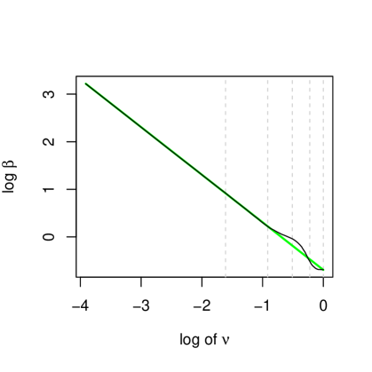
(a) log of optimal rate vs. log of $\nu$

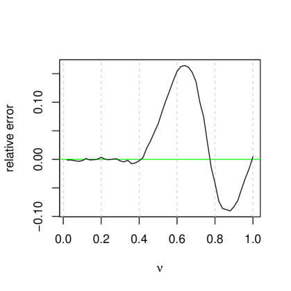
(b) relative error of optimal rate vs. $\nu$

Figure 2: Plotting the estimated optimal rate against $\nu$. The proposed optimal rate $\beta=\frac{1}{2\nu}$ (green) is also included for comparison. The grey broken lines represents grid lines for $\nu$={0, 0.2, 0.4, 0.6, 0.8, 1}. The relative error is also calculated and plotted using the formula $\frac{\hat{\beta}-\beta}{\beta}$.

In Figure 2, the optimal rate estimate in the simulation appears to follow the proposed optimal rate when $0<\nu\leq 0.4$. However when $0.4<\nu<1$, the optimal rate estimate appears slightly different with a sinusoidal pattern. In fact for $0.4<\nu\leq 0.76$, optimal rate estimate appears to be greater than the proposed optimal rate. As $\nu$ approaches to 1, the optimal rate estimate approaches the convergence rate for asymptotic normality. Although for $0.76\leq\nu<1$, optimal rate estimate appears to be less than the proposed optimal rate which contradicts the main theorem. The reason for this is yet to be known. So to investigate this unusual behaviour further, we need to analyse the asymptotic distribution from the simulation study.

5.2 Asymptotic distribution

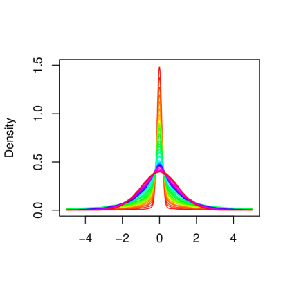
Figure 3: Density plots of the simulated $n^{\hat{\beta}}\hat{\mu}_{n}$ with its scale standardised using IQR for each $\nu$ where $n=10000$. We use a rainbow colour scheme ranging from red ($\nu$=0.02) to magenta ($\nu$=1).

In Figure 3, we plot the kernel density estimation of the simulated $n^{\hat{\beta}}\hat{\mu}_{n}$’s with its scale standardised using IQR and $n=10000$ for each $\nu$ using a Gaussian kernel. Notice that it exhibits heavier tails and sharper peaks at the expense of intermediate tails as $\nu$ decreases, which has similar behaviour to the VG distribution. We will test this claim by applying the ECM algorithm to fit the simulated $n^{\hat{\beta}}\hat{\mu}_{n}$ to the VG distribution for each pair $(\nu,n)$, then observe the Q-Q plots.

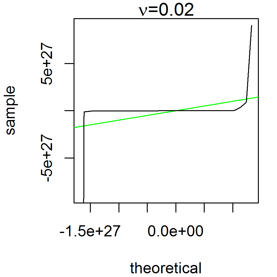
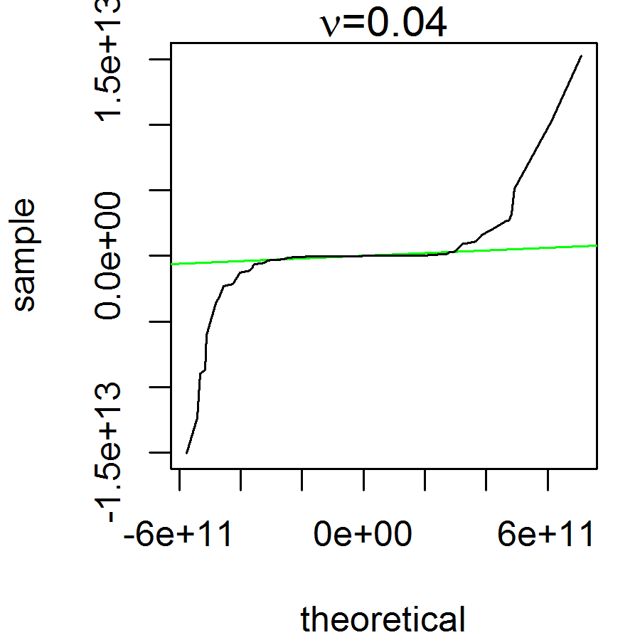
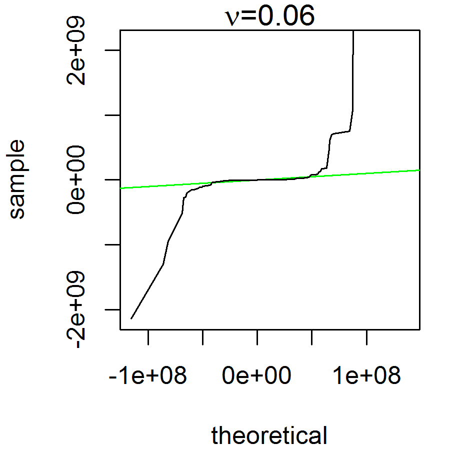
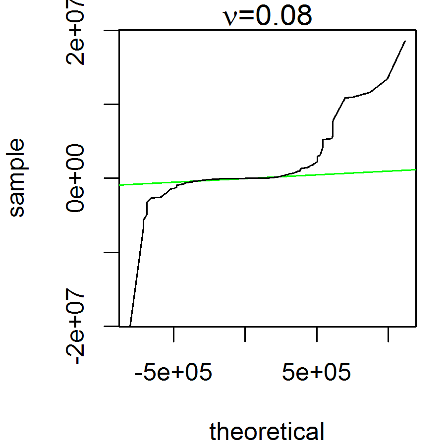
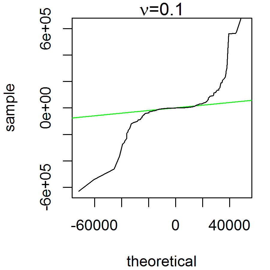
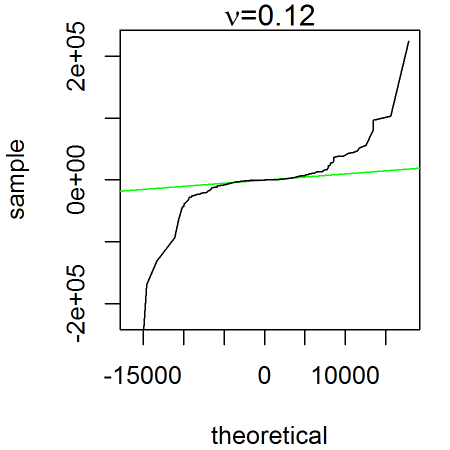
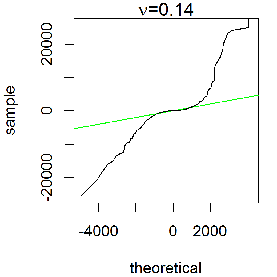
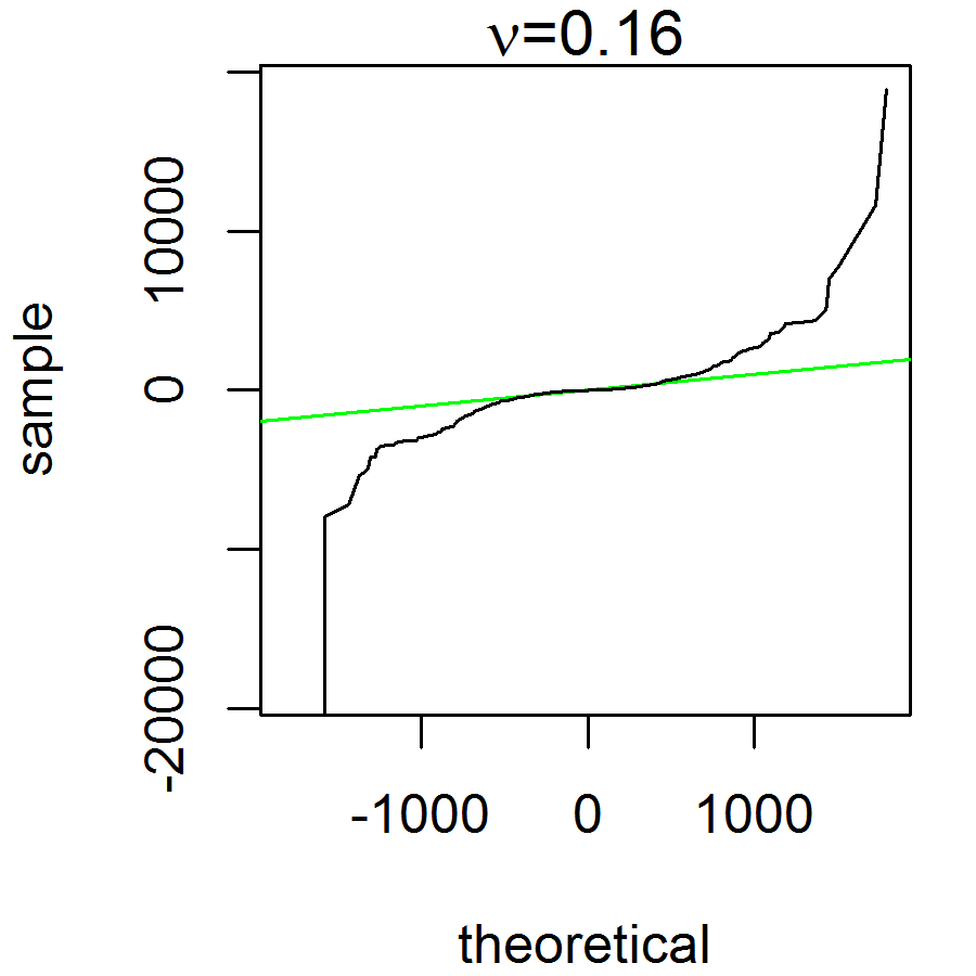
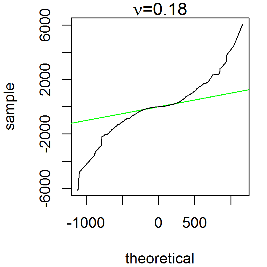
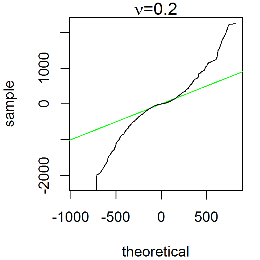
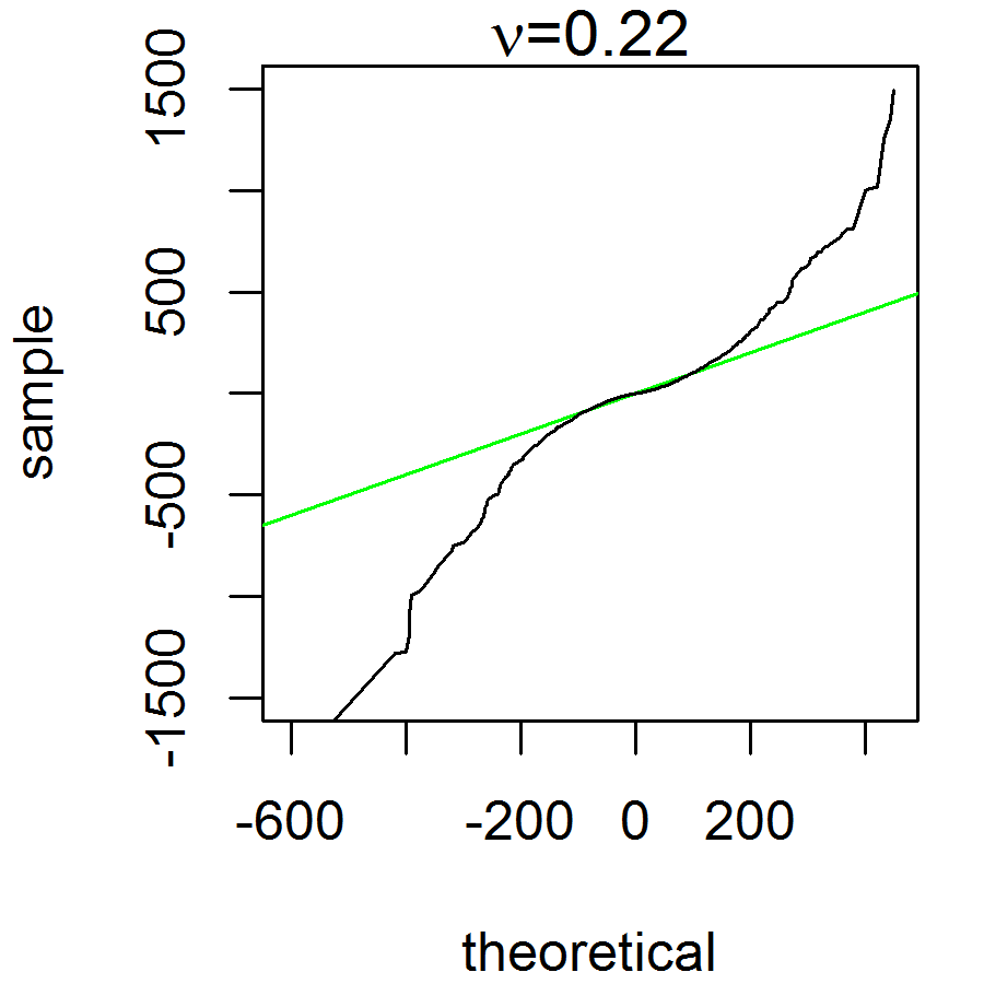
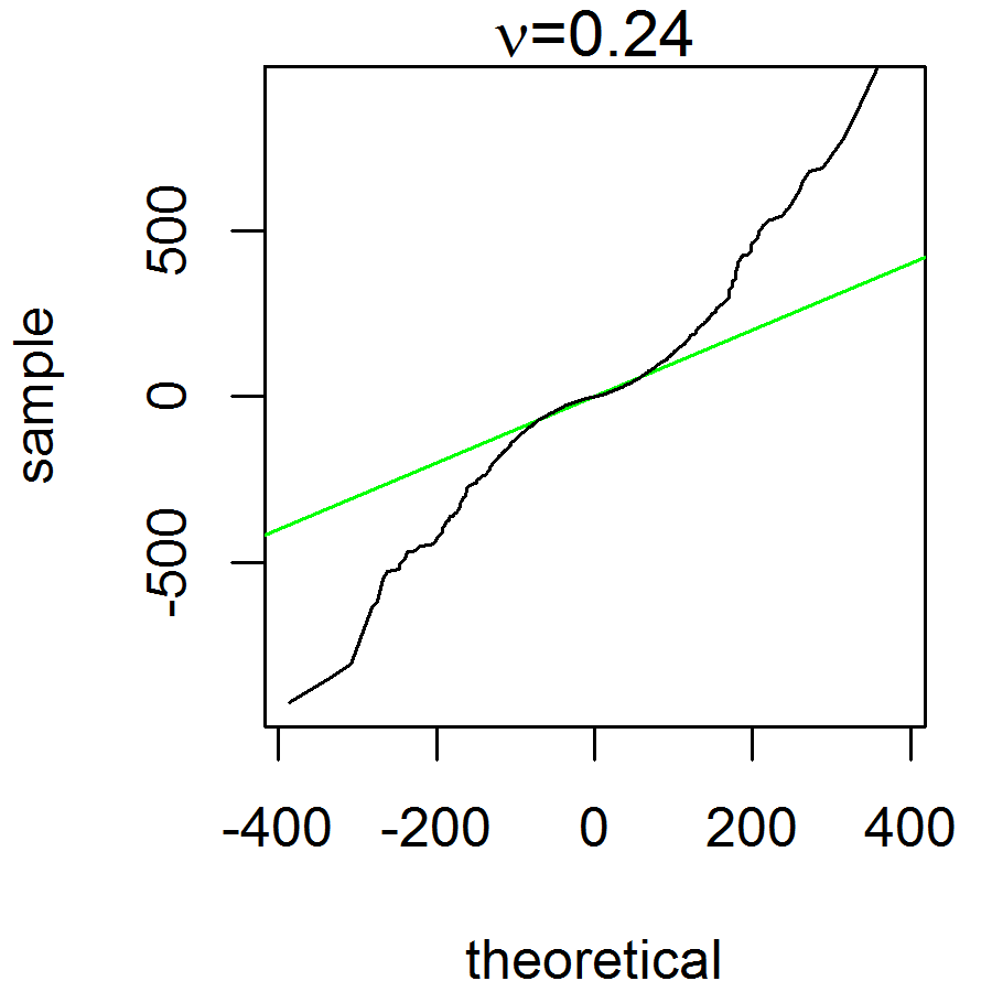
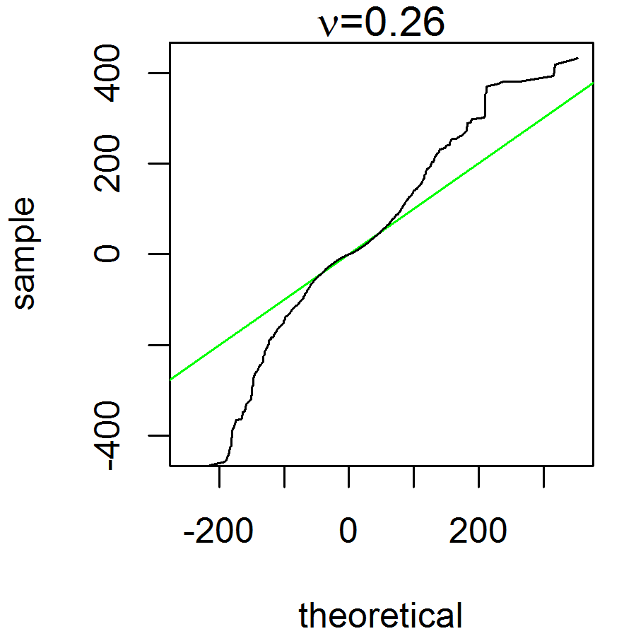
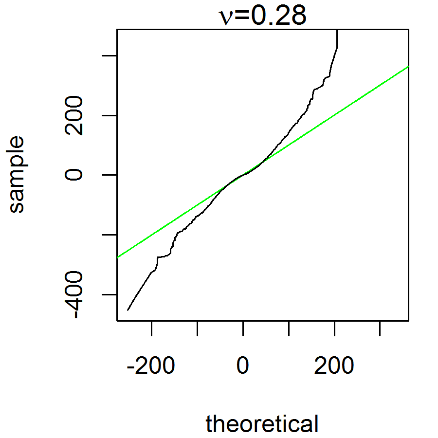
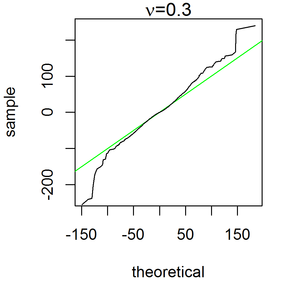
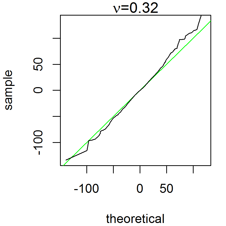
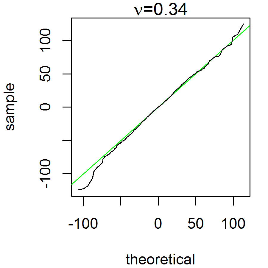
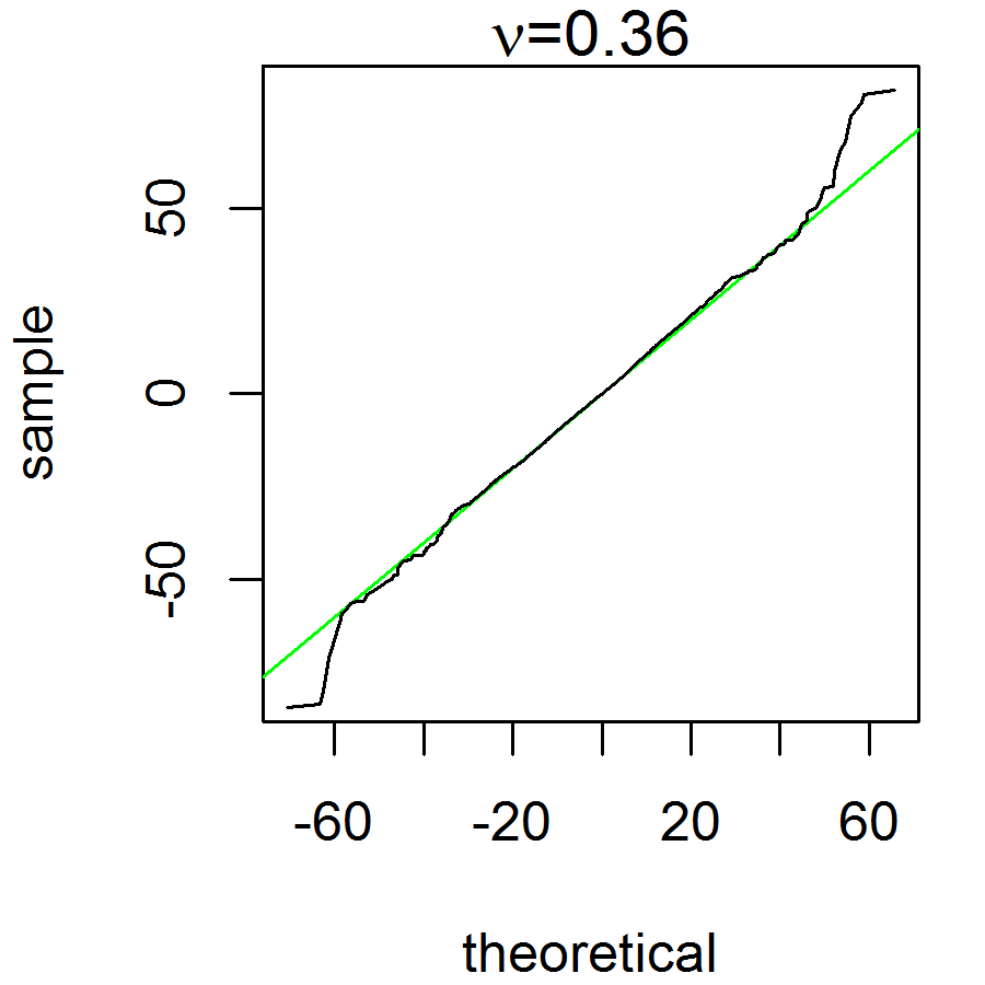
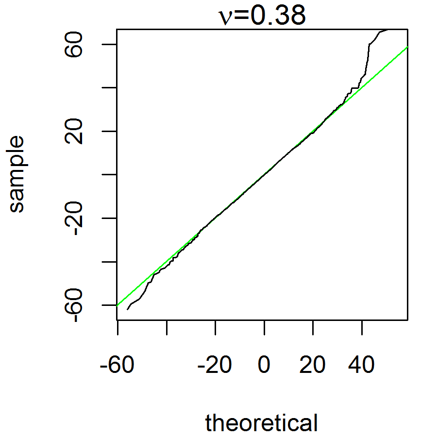
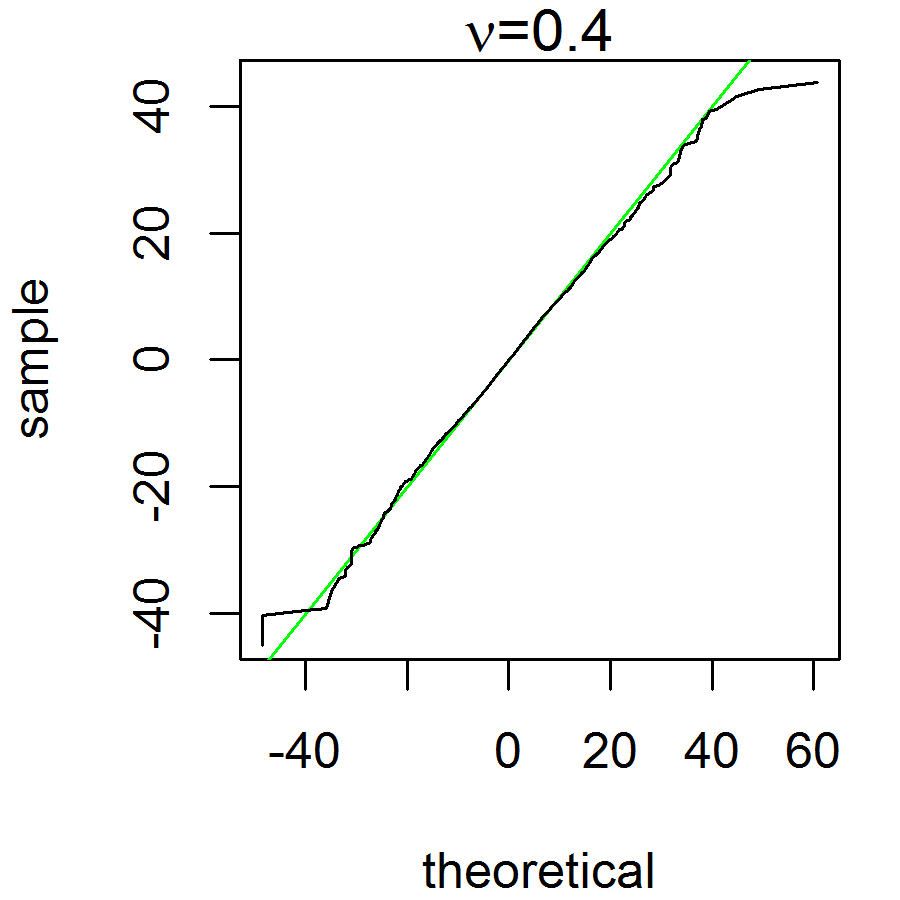
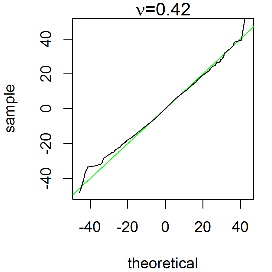
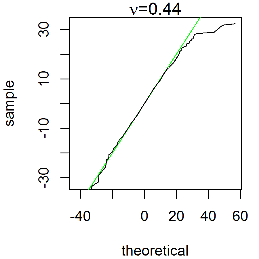
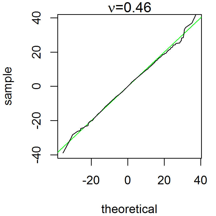
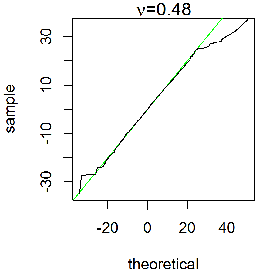
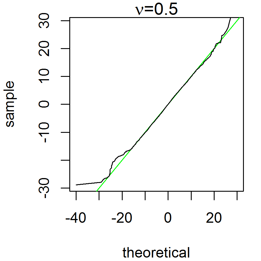
Figure 5: Q-Q plots for $0.02\leq\nu\leq 0.5$ where the x-axis represent the theoretical distribution based on ordered monte carlo sample from estimated VG distribution with scale and shape parameters $(\sigma_{\hat{\mu}},\nu_{\hat{\mu}})$, and y-axis represents the ordered $n^{\hat{\beta}}\mu_{n}$ samples for $n=10000$.

Let us denote the VG scale and shape parameter estimates of $n^{\hat{\beta}}\hat{\mu}_{n}$ to be $(\sigma_{\hat{\mu}},\nu_{\hat{\mu}})$. For simplicity, we will set the location and skewness parameter to be 0 when applying the ECM algorithm to reduce the number of parameters. The Q-Q plots is generated empirically by plotting the ordered monte carlo samples of size 20000 from the estimated VG distribution with scale and shape parameters $(\sigma_{\hat{\mu}},\nu_{\hat{\mu}})$ against the ordered simulated $n^{\hat{\beta}}{\hat{\mu}}_{n}$ for $n=10000$. Note that we only plot for $n=10000$ as the other sample sizes exhibits similar distributional behaviour. The plots and tables of the VG estimates of $n^{\hat{\beta}}\hat{\mu}_{n}$ is given in Figure 4 and Table 1 and 2 respectively, and the Q-Q plots is given in Figure 5 and 6.

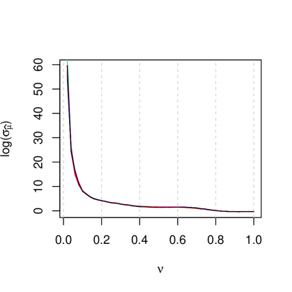
(a) $\nu$ vs. estimated log$(\sigma_{\hat{\mu}})$ of $n^{\hat{\beta}}{\hat{\mu}}_{n}$

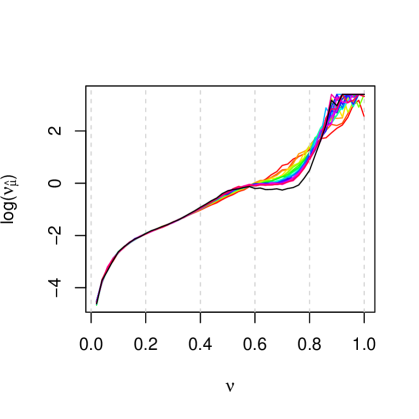
(b) $\nu$ vs. estimated log$(\nu_{\hat{\mu}})$ of $n^{\hat{\beta}}{\hat{\mu}}_{n}$

Figure 4: Plots of $\nu$ against estimates of VG distribution fitted to $n^{\hat{\beta}}{\hat{\mu}}_{n}$. We use a rainbow colour scheme ranging from red (n=500) to magenta (n=10000). Additionally, we have a black line to represent n=20000.

In Figure 4(a), $\log\sigma_{\hat{\mu}}$ roughly follows a power law with respect to $\nu$, and the scale estimate seems to be consistent for each $n$. Whereas in Figure 4(b), the shape estimate seems to be consistent for each $n$ only when $0<\nu<0.4$. However when $0.4\leq\nu\leq 1$, there seems to be considerable inconsistencies. This suggest that the rate of convergence in distribution of $n^{\hat{\beta}}\mu_{n}$ is slower for larger $\nu$ compared with smaller $\nu$. In terms of the trend of the plot, $\log\nu_{\hat{\mu}}$ roughly follows an linear trend in the range $\nu>0.2$ for $n=500$, but curves as $n$ increases.

For additional comparison, we also generated simulation results for $n=20000$ and plotted the estimated VG parameters of the simulated $n^{\hat{\beta}}{\hat{\mu}}_{n}$ in Figure 4 represented using a black line. As expected, $\sigma_{\hat{\mu}}$ is consistent with other sample sizes. However, $\nu_{\hat{\mu}}$ curves even more for $\nu>0.4$. So the slow convergence in distribution might be a possible reason why the estimated optimal rate differ with the proposed optimal rate for $0.4<\nu<1$. In spite of that, analytically finding the optimal rate of convergence requires further research.

From Figure 5 and 6, it appears that the VG distribution fits the asymptotic distributions reasonably well for $0.34\leq\nu\leq 1$ since the Q-Q plots roughly follow a straight line. As for $\nu\leq 0.32$, the asymptotic distributions appears to have heavier tails and higher density at the centre than VG distribution as $\nu$ decreases. More studies are needed to determine which distribution can approximately fit the asymptotic distribution for the whole range of $\nu$. Nevertheless, we can construct confidence intervals and approximate standard errors for the location parameter of VG distribution where we use the estimated VG distribution for $\nu\geq 0.34$, and the simulated $n^{\hat{\beta}}\hat{\mu}_{n}$ samples for $\nu<0.34$.

6 Conclusion

We have proposed an ECM algorithm to accurately estimate parameters from VG distribution while also dealing with the unbounded densities using the LOO likelihood. The maximum LOO likelihood estimator exhibits consistency and super-efficiency proved by Podgórski and Wallin, (2015). We provided simulation results to understand empirically other asymptotic properties such as the optimal rate of convergence and asymptotic distribution of the maximum LOO likelihood location estimator, however proving these asymptotic results analytically is still an open question. Nevertheless, we can construct confidence intervals and approximate standard errors for location parameter of VG distribution using the results in Section 5. Although we only implemented the univariate symmetric case in this paper, the algorithm works well for multivariate skewness case at the expense of additional computation time.

For further research, it is worth considering the asymptotic distribution with skewness and higher dimensions, or more generally the joint asymptotic distribution and the dependence between the location and other parameters from MSVG distribution. For more complicated models, finding numerical techniques for estimating the standard error and approximating the asymptotic distribution with the presence of unboundedness to capture strong leptokurtosis is important in real world applications.

The methodology presented in Section 4 can also be used for estimating parameters from other cusped, unbounded, or even distributions with extreme leptokurtosis such as stable distribution with small stable index, or leptokurtic financial models for high frequency data (Kawai,, 2015).

Appendix Appendix

Table 1: optimal rate estimates, proposed optimal rate, and $(\sigma_{\hat{\mu}},\nu_{\hat{\mu}})$ values for $0.02\leq\nu\leq 0.5$ and for selected $n=\{500,3000,7000,10000,20000\}$.

$\nu$	$\hat{\beta}$	$\beta$	$\sigma_{\hat{\mu}}$	$\nu_{\hat{\mu}}$
0.02	24.95	25.00	$10^{24}\begin{pmatrix}1.4&1.2&0.3&72&81\end{pmatrix}$	$10^{-2}\begin{pmatrix}1.1&1.1&1.1&1.0&1.0\end{pmatrix}$
0.04	12.46	12.50	$10^{10}\begin{pmatrix}6.4&17&6.5&3.1&4.4\end{pmatrix}$	$10^{-2}\begin{pmatrix}2.4&2.3&2.4&2.5&2.4\end{pmatrix}$
0.06	8.32	8.33	$10^{6}\begin{pmatrix}5.1&8.1&8.6&5.3&19\end{pmatrix}$	$10^{-2}\begin{pmatrix}3.9&3.7&3.7&3.9&3.5\end{pmatrix}$
0.08	6.23	6.25	$10^{4}\begin{pmatrix}11&6.2&4.4&5.3&8.9\end{pmatrix}$	$10^{-2}\begin{pmatrix}5.0&5.4&5.5&5.5&5.2\end{pmatrix}$
0.1	4.97	5.00	$10^{3}\begin{pmatrix}3.7&3.4&3.8&3.6&3.0\end{pmatrix}$	$10^{-2}\begin{pmatrix}7.1&7.2&7.1&7.1&7.3\end{pmatrix}$
0.12	4.17	4.17	$10^{2}\begin{pmatrix}9.0&11&10&10&9.3\end{pmatrix}$	$10^{-2}\begin{pmatrix}8.8&8.5&8.6&8.7&8.8\end{pmatrix}$
0.14	3.57	3.57	$10^{2}\begin{pmatrix}3.1&3.5&3.2&2.9&3.0\end{pmatrix}$	$\begin{pmatrix}0.10&0.10&0.10&0.10&0.10\end{pmatrix}$
0.16	3.12	3.13	$10^{2}\begin{pmatrix}1.5&1.6&1.3&1.5&1.4\end{pmatrix}$	$\begin{pmatrix}0.12&0.12&0.12&0.12&0.12\end{pmatrix}$
0.18	2.78	2.78	$\begin{pmatrix}85&92&94&94&96\end{pmatrix}$	$\begin{pmatrix}0.13&0.13&0.13&0.13&0.13\end{pmatrix}$
0.2	2.51	2.50	$\begin{pmatrix}62&63&66&68&63\end{pmatrix}$	$\begin{pmatrix}0.15&0.15&0.14&0.14&0.15\end{pmatrix}$
0.22	2.29	2.27	$\begin{pmatrix}47&46&47&46&47\end{pmatrix}$	$\begin{pmatrix}0.16&0.16&0.16&0.16&0.16\end{pmatrix}$
0.24	2.08	2.08	$\begin{pmatrix}31&32&32&33&32\end{pmatrix}$	$\begin{pmatrix}0.17&0.17&0.17&0.17&0.17\end{pmatrix}$
0.26	1.92	1.92	$\begin{pmatrix}24&25&25&26&25\end{pmatrix}$	$\begin{pmatrix}0.19&0.19&0.19&0.18&0.19\end{pmatrix}$
0.28	1.79	1.79	$\begin{pmatrix}22&22&23&24&22\end{pmatrix}$	$\begin{pmatrix}0.21&0.20&0.21&0.20&0.21\end{pmatrix}$
0.3	1.65	1.67	$\begin{pmatrix}17&17&16&16&15\end{pmatrix}$	$\begin{pmatrix}0.22&0.22&0.22&0.23&0.23\end{pmatrix}$
0.32	1.54	1.56	$\begin{pmatrix}13&13&12&12&12\end{pmatrix}$	$\begin{pmatrix}0.25&0.24&0.25&0.25&0.25\end{pmatrix}$
0.34	1.45	1.47	$\begin{pmatrix}11&11&11&11&11\end{pmatrix}$	$\begin{pmatrix}0.27&0.27&0.27&0.28&0.28\end{pmatrix}$
0.36	1.35	1.39	$\begin{pmatrix}8.9&8.6&8.6&8.3&7.6\end{pmatrix}$	$\begin{pmatrix}0.30&0.31&0.30&0.31&0.31\end{pmatrix}$
0.38	1.28	1.32	$\begin{pmatrix}7.5&7.3&7.0&6.9&6.5\end{pmatrix}$	$\begin{pmatrix}0.33&0.34&0.34&0.34&0.35\end{pmatrix}$
0.4	1.21	1.25	$\begin{pmatrix}6.5&6.3&6.0&5.8&5.3\end{pmatrix}$	$\begin{pmatrix}0.36&0.38&0.37&0.39&0.40\end{pmatrix}$
0.42	1.16	1.19	$\begin{pmatrix}6.1&5.9&5.6&5.7&5.1\end{pmatrix}$	$\begin{pmatrix}0.40&0.42&0.43&0.43&0.45\end{pmatrix}$
0.44	1.12	1.14	$\begin{pmatrix}5.9&5.6&5.5&5.4&4.8\end{pmatrix}$	$\begin{pmatrix}0.44&0.47&0.50&0.48&0.51\end{pmatrix}$
0.46	1.07	1.09	$\begin{pmatrix}5.3&5.1&4.9&4.8&4.4\end{pmatrix}$	$\begin{pmatrix}0.47&0.53&0.54&0.56&0.57\end{pmatrix}$
0.48	1.04	1.04	$\begin{pmatrix}5.1&5.0&4.8&4.7&4.2\end{pmatrix}$	$\begin{pmatrix}0.53&0.60&0.63&0.63&0.67\end{pmatrix}$
0.5	1.01	1.00	$\begin{pmatrix}4.9&4.8&4.7&4.6&4.2\end{pmatrix}$	$\begin{pmatrix}0.59&0.65&0.68&0.69&0.75\end{pmatrix}$

Table 2: optimal rate estimates, proposed optimal rate, and $(\sigma_{\hat{\mu}},\nu_{\hat{\mu}})$ values for $0.52\leq\nu\leq 1$ and for selected $n=\{500,3000,7000,10000,20000\}$.

$\nu$	$\hat{\beta}$	$\beta$	$\sigma_{\hat{\mu}}$	$\nu_{\hat{\mu}}$
0.52	0.99	0.96	$\begin{pmatrix}4.7&4.8&4.7&4.5&4.1\end{pmatrix}$	$\begin{pmatrix}0.65&0.72&0.76&0.81&0.79\end{pmatrix}$
0.54	0.97	0.93	$\begin{pmatrix}4.7&4.9&4.7&4.6&4.3\end{pmatrix}$	$\begin{pmatrix}0.73&0.79&0.81&0.88&0.81\end{pmatrix}$
0.56	0.94	0.89	$\begin{pmatrix}4.5&4.8&4.6&4.6&4.2\end{pmatrix}$	$\begin{pmatrix}0.77&0.84&0.89&0.85&0.85\end{pmatrix}$
0.58	0.92	0.86	$\begin{pmatrix}4.5&4.9&4.8&4.7&4.4\end{pmatrix}$	$\begin{pmatrix}0.88&0.91&0.93&0.93&0.88\end{pmatrix}$
0.6	0.90	0.83	$\begin{pmatrix}4.4&4.8&4.8&4.8&4.4\end{pmatrix}$	$\begin{pmatrix}0.99&0.94&0.98&0.90&0.82\end{pmatrix}$
0.62	0.88	0.81	$\begin{pmatrix}4.2&4.7&4.7&4.6&4.5\end{pmatrix}$	$\begin{pmatrix}1.0&0.98&0.98&0.94&0.83\end{pmatrix}$
0.64	0.85	0.78	$\begin{pmatrix}3.8&4.3&4.3&4.4&4.1\end{pmatrix}$	$\begin{pmatrix}1.2&1.1&1.0&0.93&0.78\end{pmatrix}$
0.66	0.83	0.76	$\begin{pmatrix}3.5&4.0&4.0&4.1&3.9\end{pmatrix}$	$\begin{pmatrix}1.4&1.1&0.99&0.94&0.79\end{pmatrix}$
0.68	0.79	0.74	$\begin{pmatrix}3.0&3.5&3.6&3.6&3.5\end{pmatrix}$	$\begin{pmatrix}1.6&1.2&1.0&1.0&0.81\end{pmatrix}$
0.7	0.76	0.71	$\begin{pmatrix}2.6&3.1&3.2&3.2&3.2\end{pmatrix}$	$\begin{pmatrix}2.0&1.3&1.1&1.0&0.77\end{pmatrix}$
0.72	0.72	0.69	$\begin{pmatrix}2.1&2.4&2.4&2.4&2.5\end{pmatrix}$	$\begin{pmatrix}2.1&1.5&1.2&1.0&0.82\end{pmatrix}$
0.74	0.69	0.68	$\begin{pmatrix}1.8&2.1&2.2&2.2&2.2\end{pmatrix}$	$\begin{pmatrix}2.5&1.9&1.2&1.1&0.85\end{pmatrix}$
0.76	0.65	0.66	$\begin{pmatrix}1.4&1.6&1.7&1.7&1.7\end{pmatrix}$	$\begin{pmatrix}2.8&2.1&1.5&1.4&0.93\end{pmatrix}$
0.78	0.61	0.64	$\begin{pmatrix}1.2&1.3&1.3&1.3&1.4\end{pmatrix}$	$\begin{pmatrix}3.0&2.5&1.8&1.8&1.2\end{pmatrix}$
0.8	0.59	0.63	$\begin{pmatrix}1.1&1.1&1.1&1.1&1.2\end{pmatrix}$	$\begin{pmatrix}3.6&3.3&2.5&2.5&1.6\end{pmatrix}$
0.82	0.56	0.61	$\begin{pmatrix}0.92&0.93&0.94&0.95&0.95\end{pmatrix}$	$\begin{pmatrix}4.2&4.6&3.5&3.7&2.9\end{pmatrix}$
0.84	0.54	0.60	$\begin{pmatrix}0.83&0.83&0.84&0.84&0.84\end{pmatrix}$	$\begin{pmatrix}5.5&6.9&5.6&5.4&5.1\end{pmatrix}$
0.86	0.53	0.58	$\begin{pmatrix}0.80&0.78&0.78&0.78&0.78\end{pmatrix}$	$\begin{pmatrix}5.7&8.4&7.4&12&9.3\end{pmatrix}$
0.88	0.51	0.57	$\begin{pmatrix}0.74&0.72&0.72&0.72&0.72\end{pmatrix}$	$\begin{pmatrix}6.9&12&16&17&24\end{pmatrix}$
0.9	0.51	0.56	$\begin{pmatrix}0.74&0.73&0.73&0.73&0.73\end{pmatrix}$	$\begin{pmatrix}8.2&13&15&17&19\end{pmatrix}$
0.92	0.50	0.54	$\begin{pmatrix}0.71&0.69&0.69&0.69&0.67\end{pmatrix}$	$\begin{pmatrix}9.3&30&25&30&30\end{pmatrix}$
0.94	0.51	0.53	$\begin{pmatrix}0.73&0.72&0.72&0.71&0.72\end{pmatrix}$	$\begin{pmatrix}12&30&30&22&30\end{pmatrix}$
0.96	0.50	0.52	$\begin{pmatrix}0.73&0.72&0.72&0.73&0.72\end{pmatrix}$	$\begin{pmatrix}20&30&30&24&30\end{pmatrix}$
0.98	0.50	0.51	$\begin{pmatrix}0.73&0.72&0.71&0.72&0.72\end{pmatrix}$	$\begin{pmatrix}24&18&30&30&30\end{pmatrix}$
1	0.50	0.50	$\begin{pmatrix}0.74&0.73&0.73&0.73&0.72\end{pmatrix}$	$\begin{pmatrix}13&30&30&28&30\end{pmatrix}$

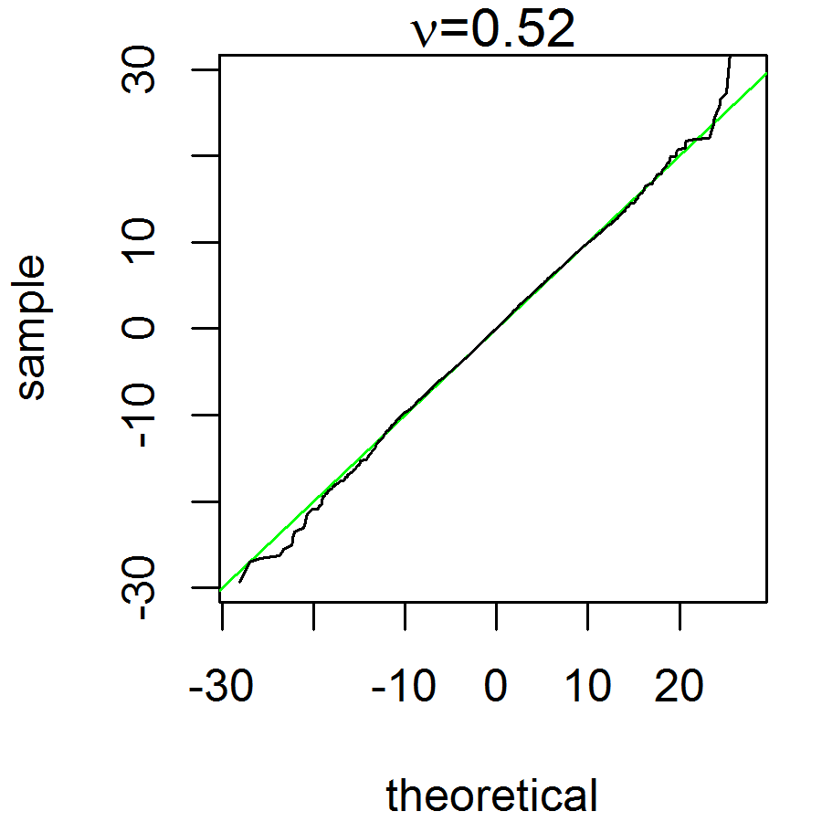
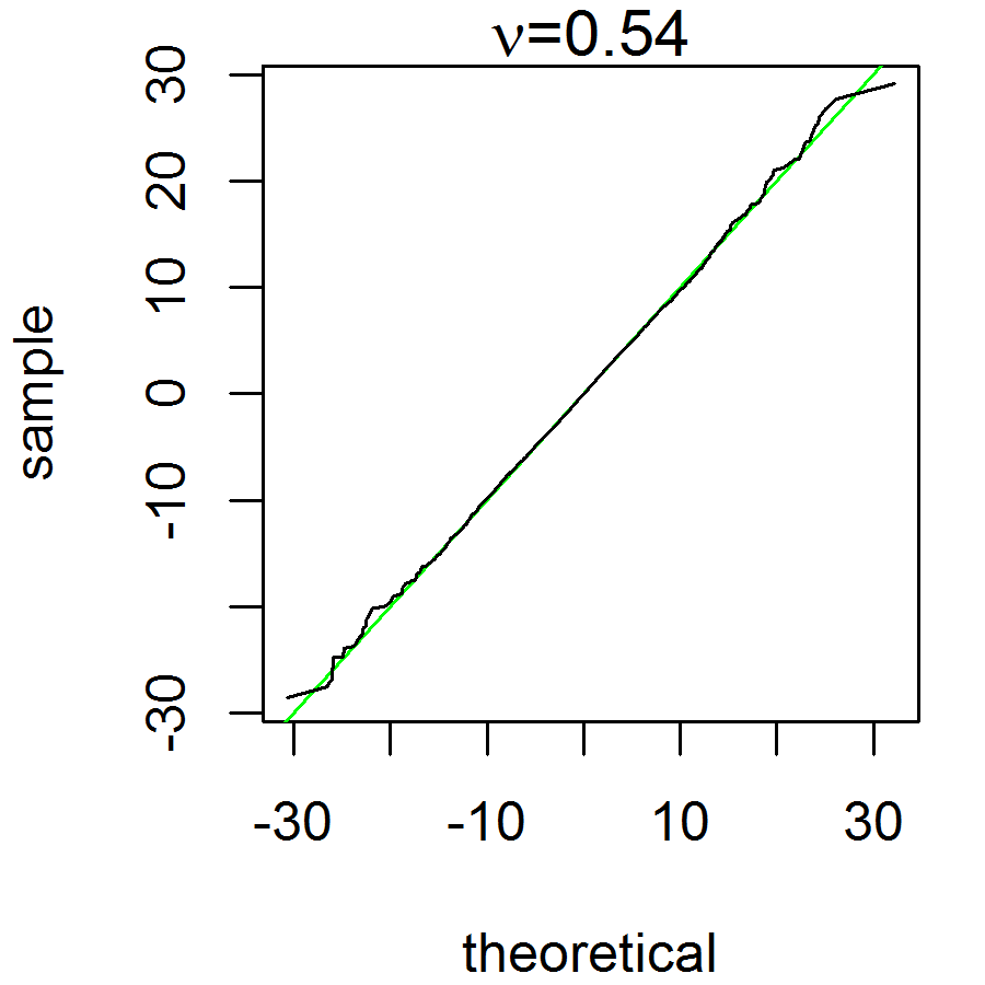
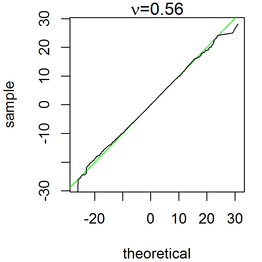
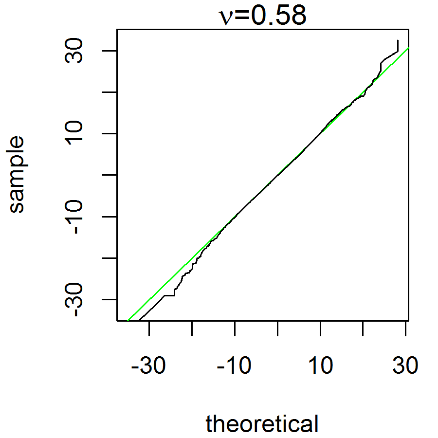
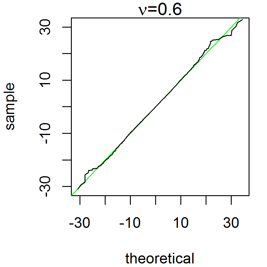
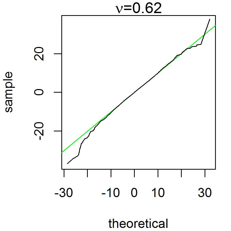
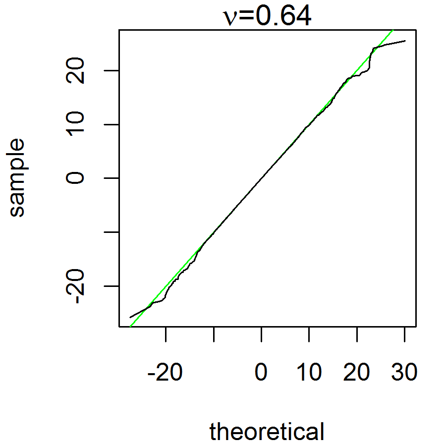
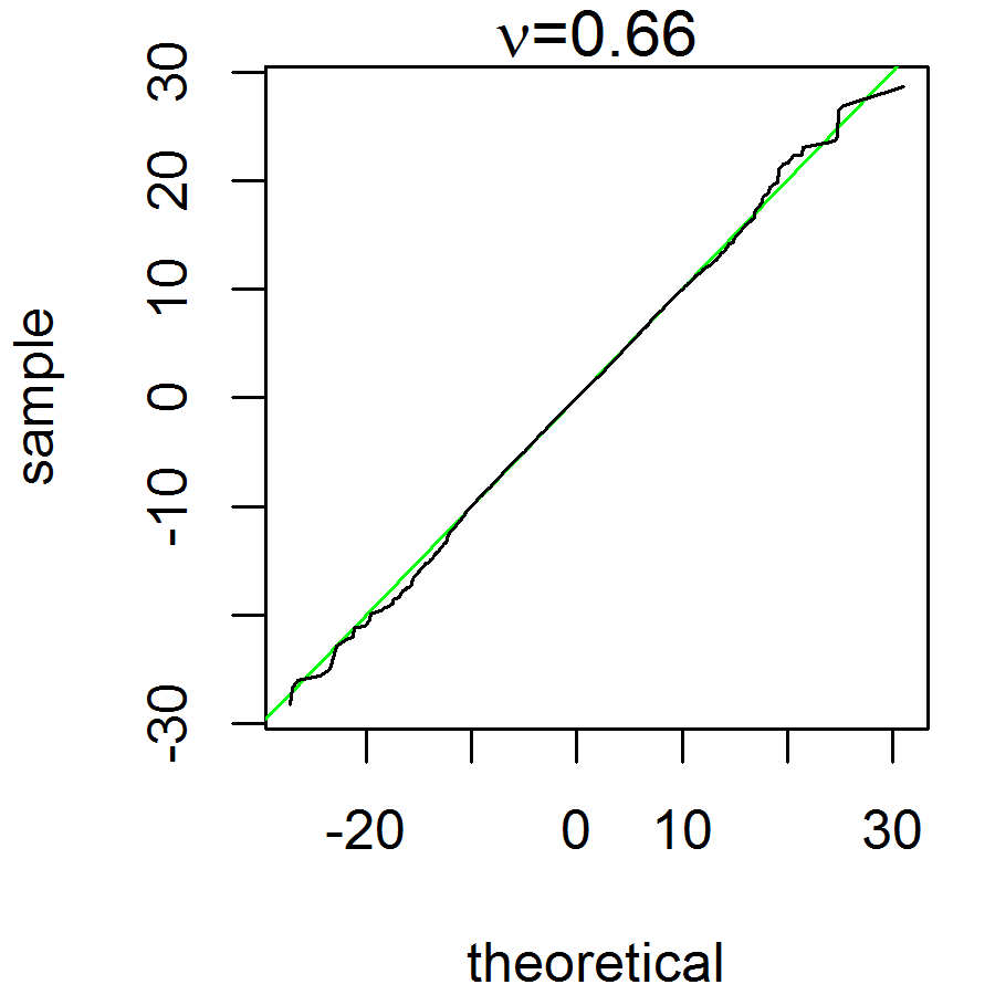
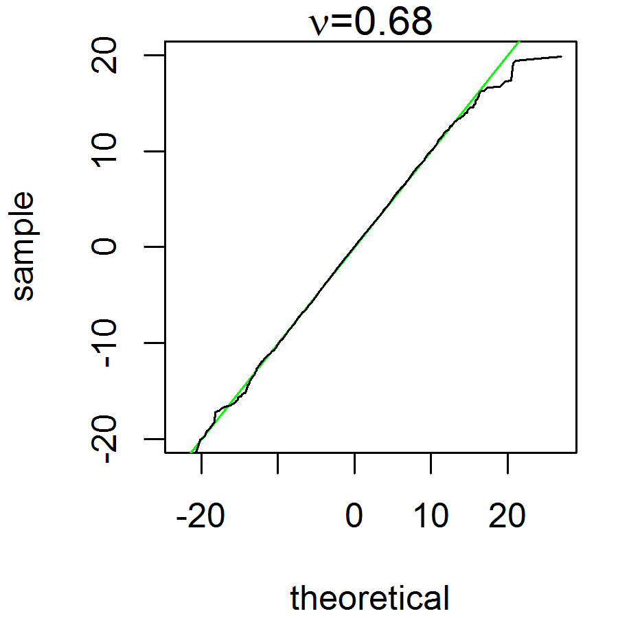
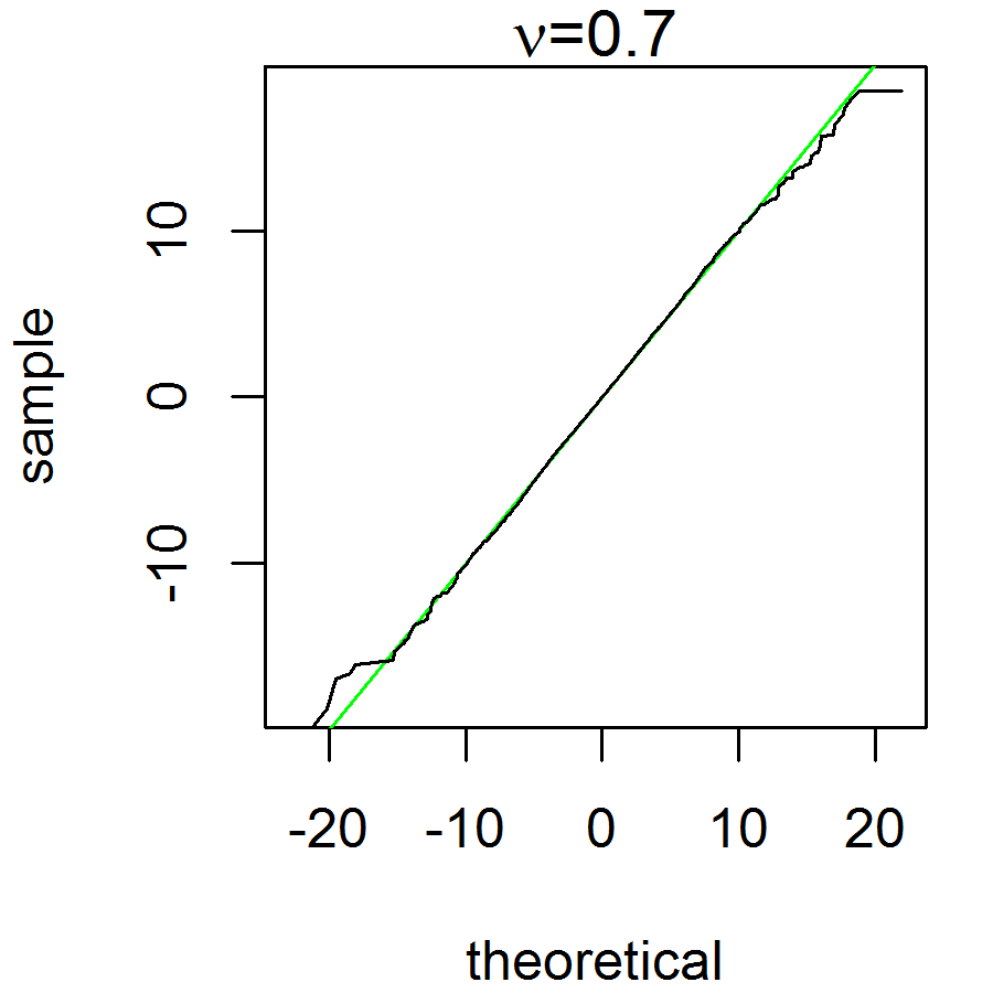
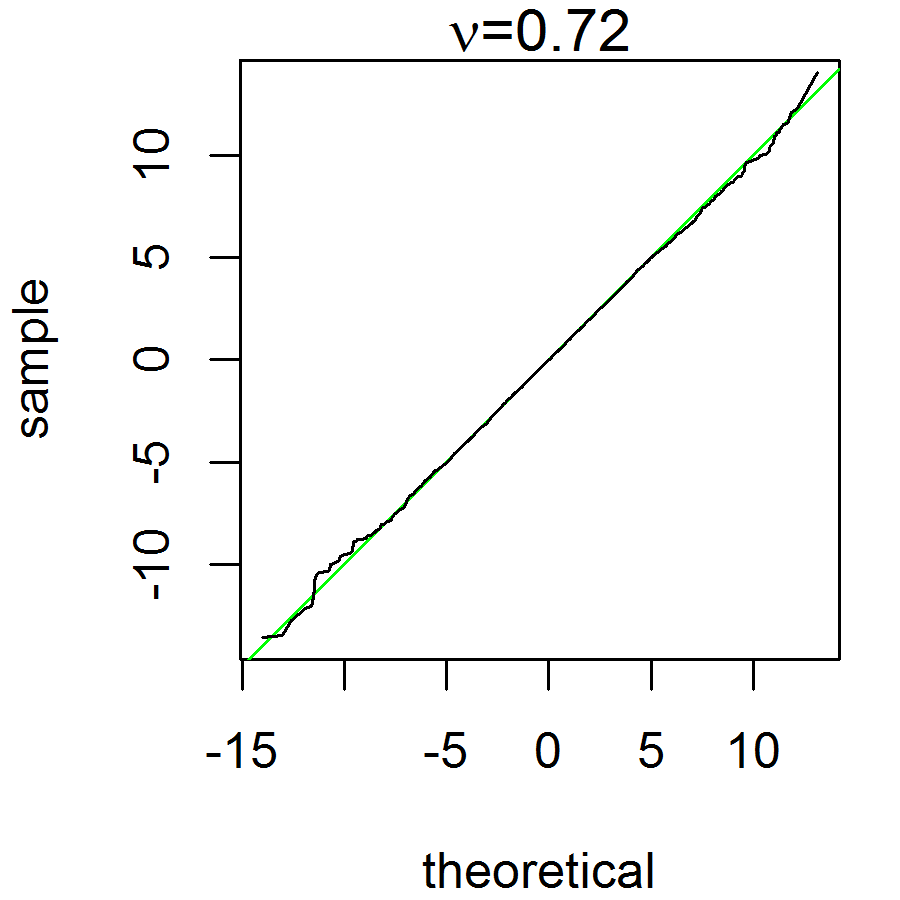
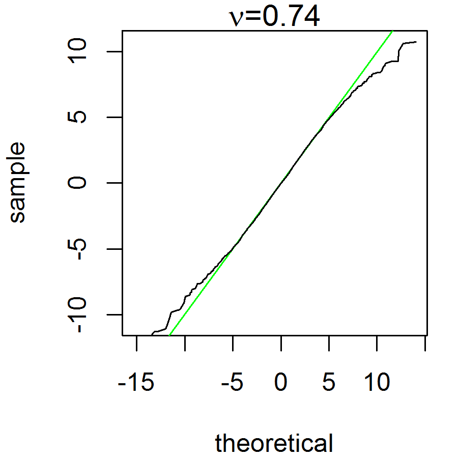
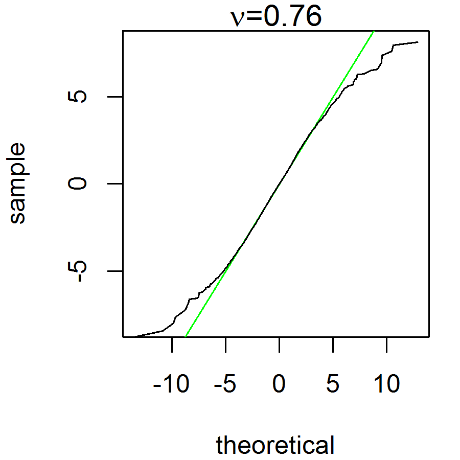
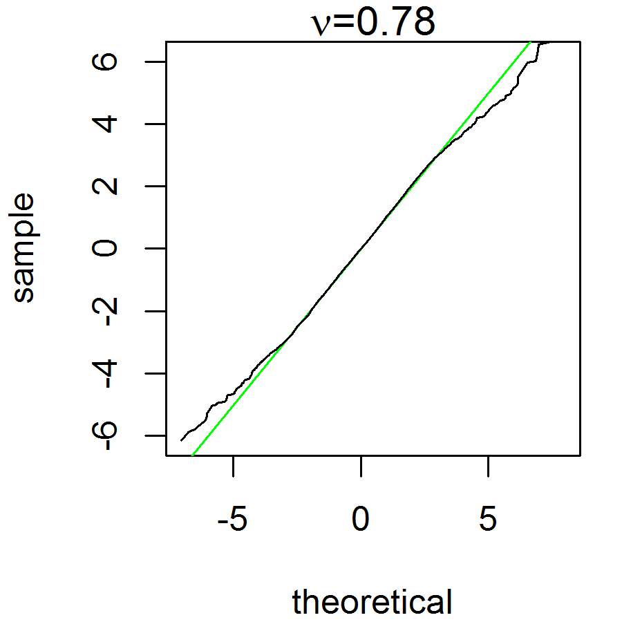
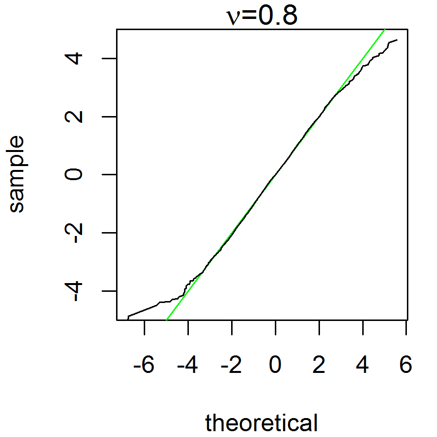
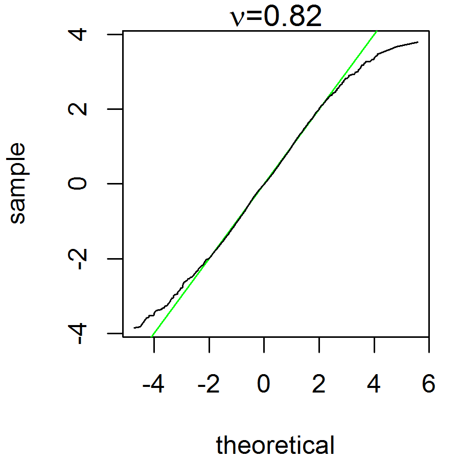
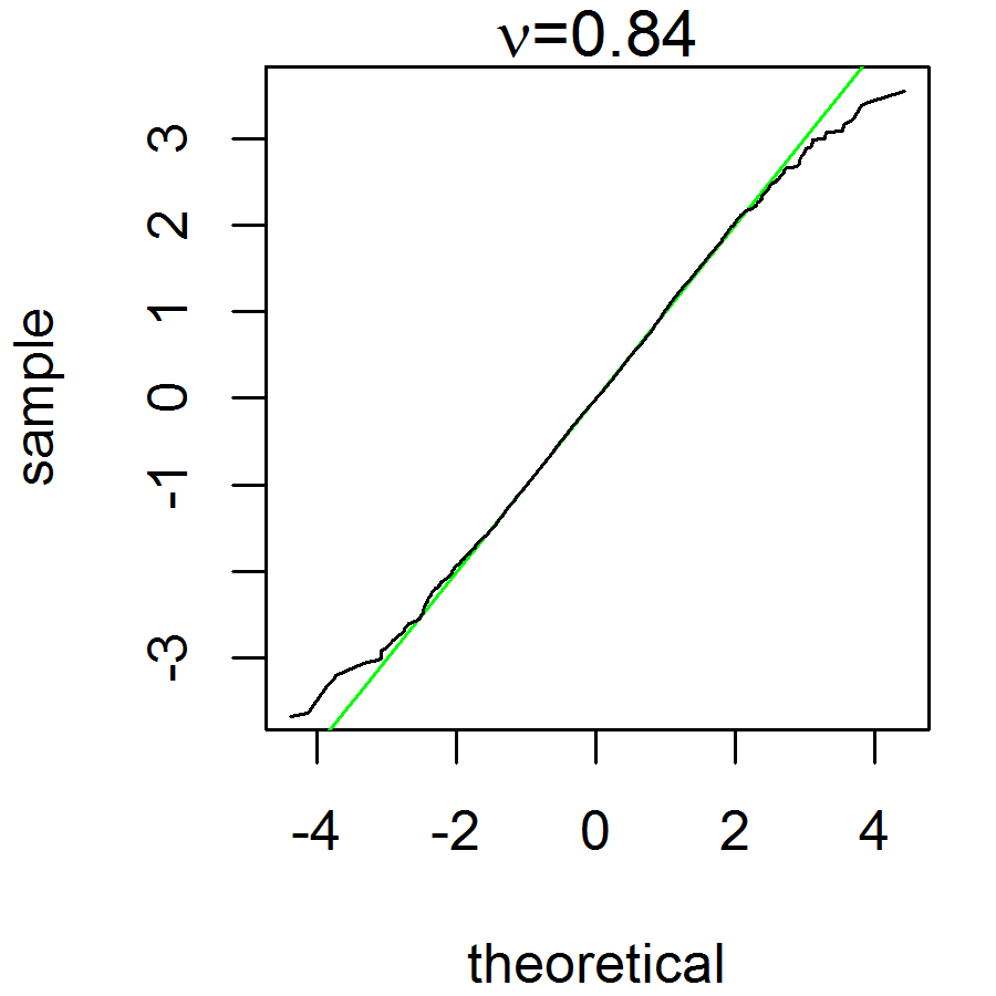
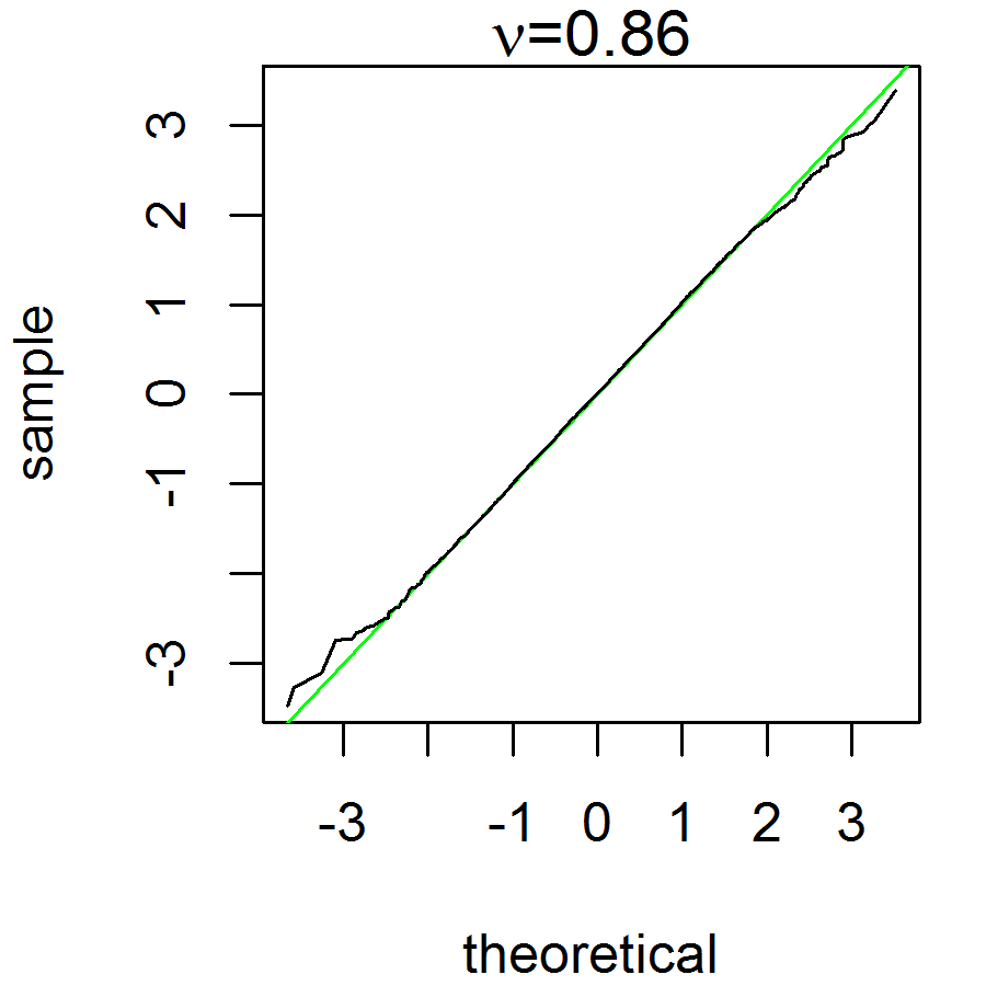
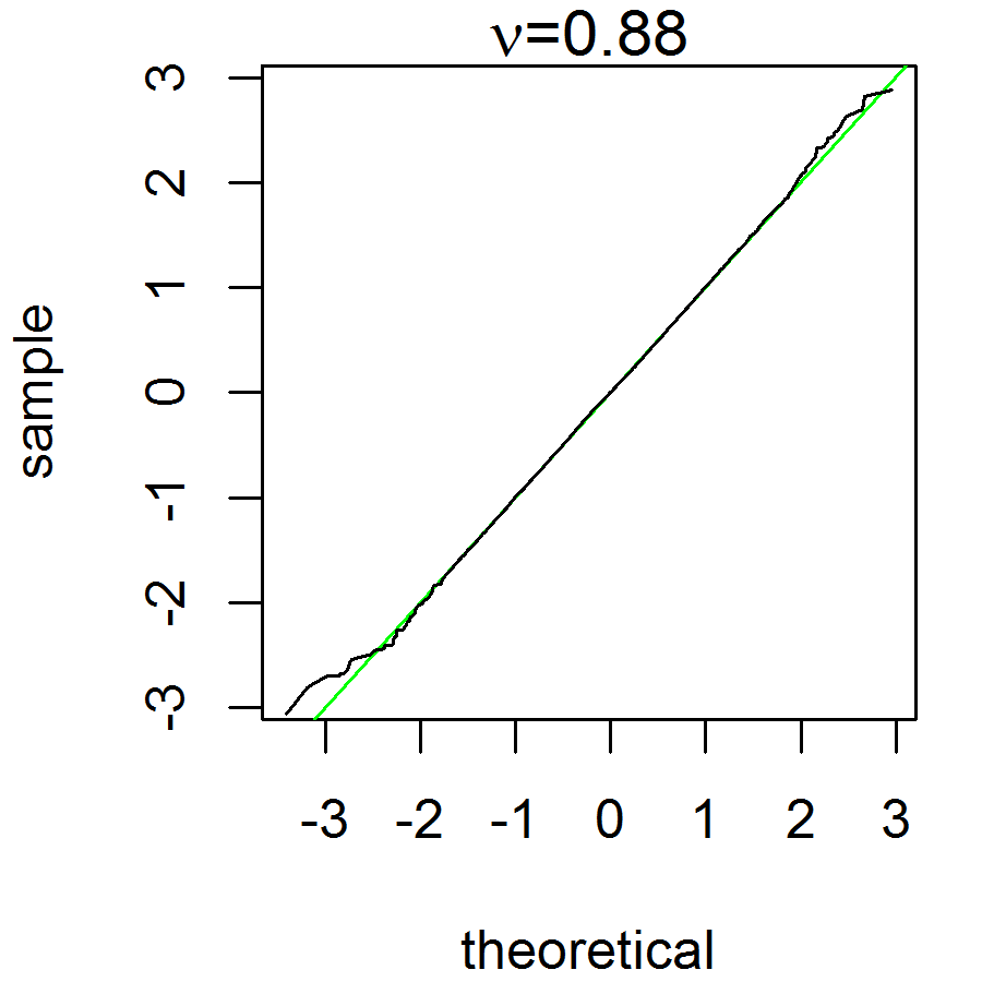
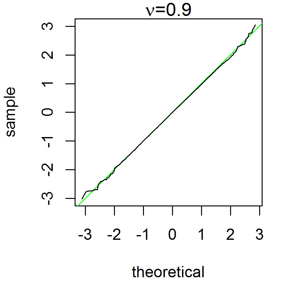
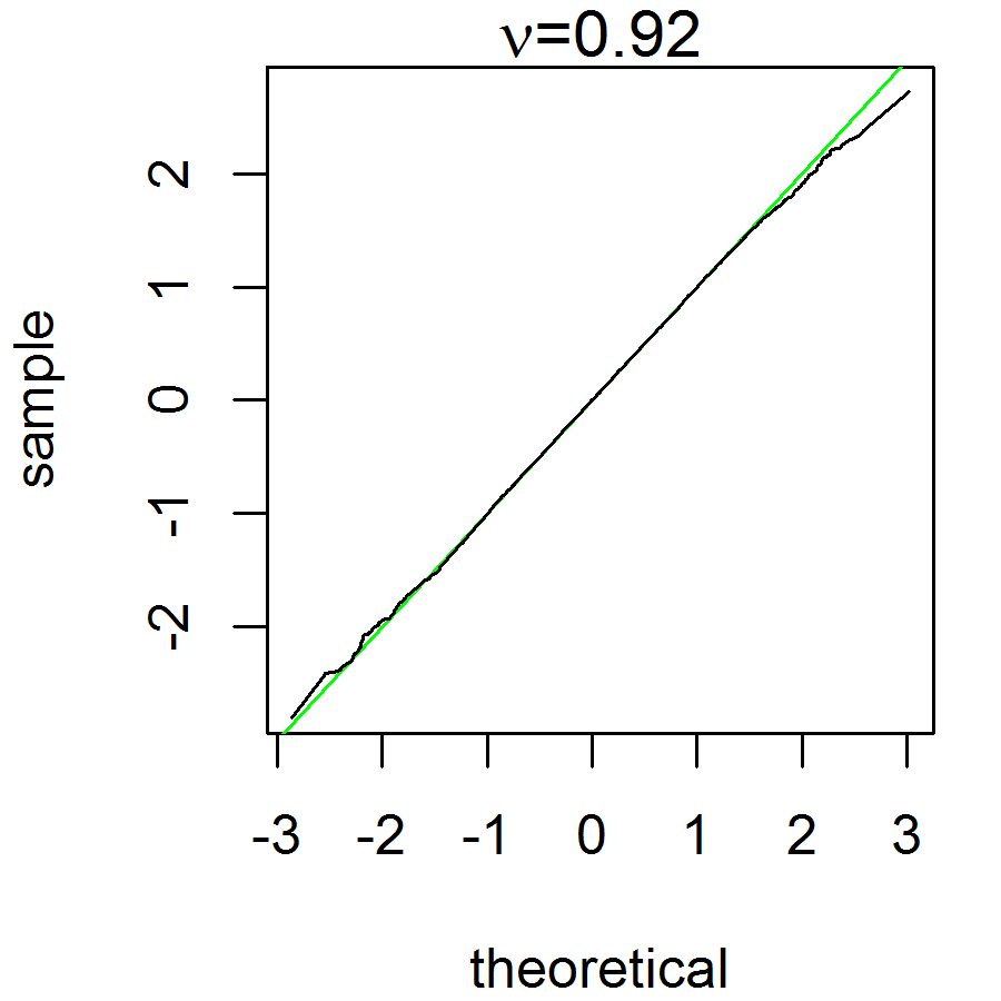
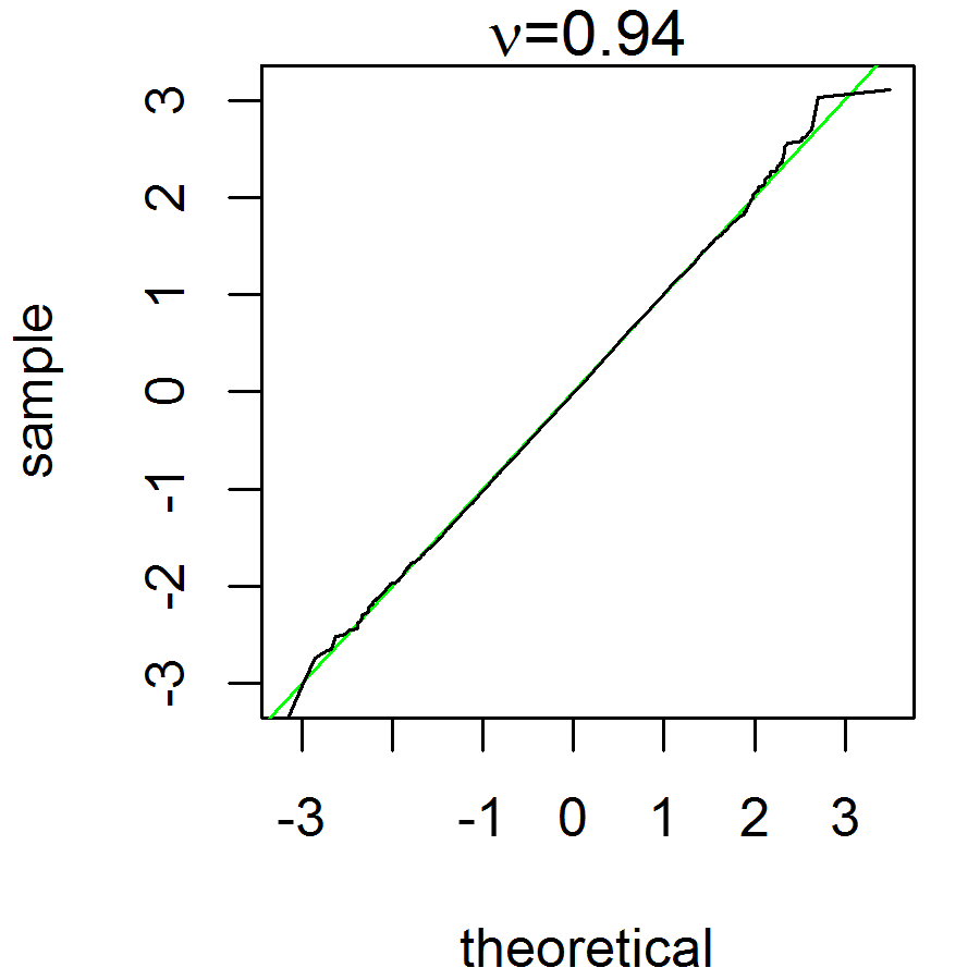
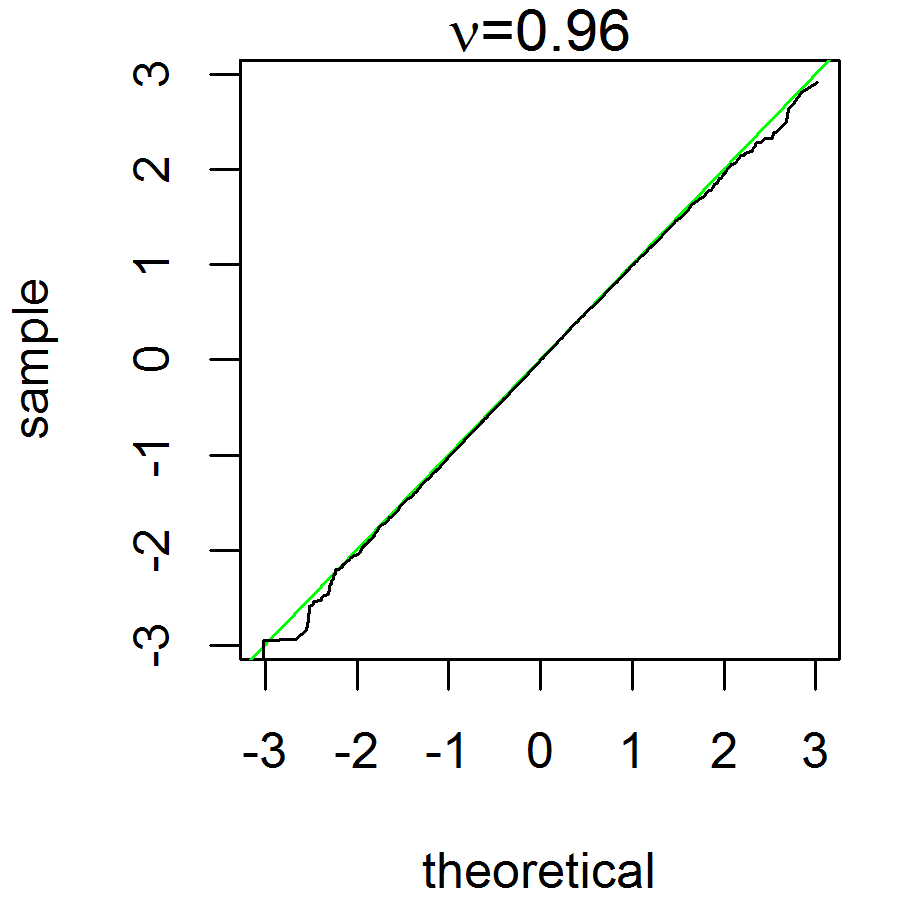
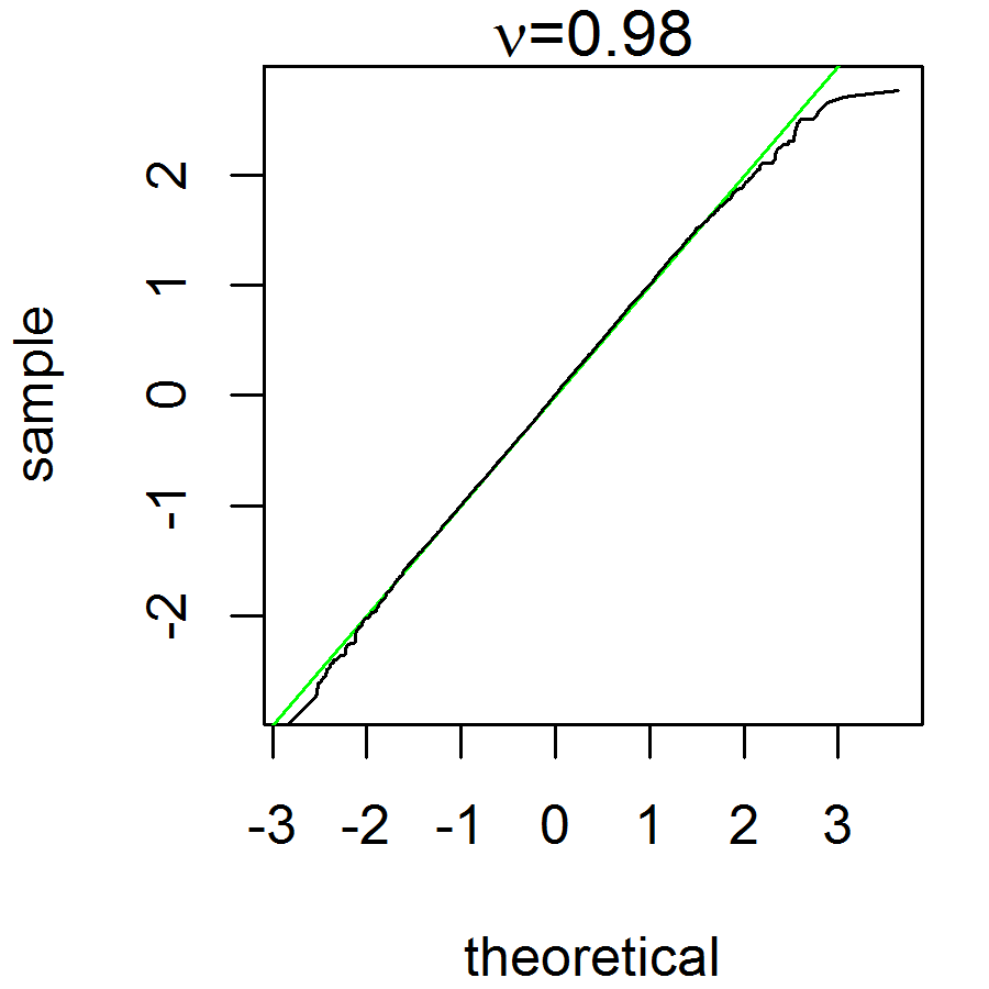
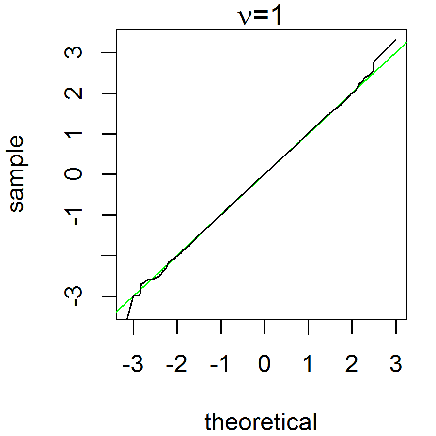
Figure 6: Q-Q plots for $0.52\leq\nu\leq 1$.

References

- Barndorff-Nielsen et al., (1982) Barndorff-Nielsen, O., Kent, J., and Sørensen, M. (1982). Normal variance-mean mixtures and distributions. Internat. Statist. Rev., 50(2):145–159.
- Dempster et al., (1977) Dempster, A. P., Laird, N. M., and Rubin, D. B. (1977). Maximum likelihood from incomplete data via the EM algorithm. J. Roy. Statist. Soc. Ser. B, 39(1):1–38. With discussion.
- Embrechts, (1983) Embrechts, P. (1983). A property of the generalized inverse Gaussian distribution with some applications. J. Appl. Probab., 20(3):537–544.
- Gradshteyn and Ryzhik, (2007) Gradshteyn, I. S. and Ryzhik, I. M. (2007). Table of integrals, series, and products. Elsevier/Academic Press, Amsterdam, seventh edition.
- (5) Ibragimov, I. A. and Khasminskii, R. Z. (1981a). Asymptotic behavior of statistical estimates of the location parameter for samples with unbounded density. J. Sov. Math., 16(2):1035–1041.
- (6) Ibragimov, I. A. and Khasminskii, R. Z. (1981b). Statistical estimation, volume 16 of Applications of Mathematics. Springer-Verlag, New York-Berlin. Asymptotic theory, Translated from the Russian by Samuel Kotz.
- Kawai, (2015) Kawai, R. (2015). On the likelihood function of small time variance gamma Lévy processes. Statistics, 49(1):63–83.
- Kotz et al., (2001) Kotz, S., Kozubowski, T. J., and Podgórski, K. (2001). The Laplace distribution and generalizations : a revisit with applications to communications, economics, engineering, and finance. Birkhäuser, Boston.
- Madan and Seneta, (1990) Madan, D. B. and Seneta, E. (1990). The variance gamma (V.G.) model for share market returns. J. Bus., 63(4):511–524.
- Meng and Rubin, (1993) Meng, X.-L. and Rubin, D. B. (1993). Maximum likelihood estimation via the ECM algorithm: a general framework. Biometrika, 80(2):267–278.
- Nitithumbundit and Chan, (2015) Nitithumbundit, T. and Chan, J. S. (2015). An ECM algorithm for skewed multivariate variance gamma distribution in normal mean-variance representation. arXiv preprint arXiv:1504.01239.