$k$-variates++: more pluses in the $k$-means++

Abstract

$k$-means++ seeding has become a de facto standard for hard clustering algorithms. In this paper, our first contribution is a two-way generalisation of this seeding, $k$-variates++, that includes the sampling of general densities rather than just a discrete set of Dirac densities anchored at the point locations, and a generalisation of the well known Arthur-Vassilvitskii (AV) approximation guarantee, in the form of a bias+variance approximation bound of the global optimum. This approximation exhibits a reduced dependency on the ”noise” component with respect to the optimal potential — actually approaching the statistical lower bound. We show that $k$-variates++ reduces to efficient (biased seeding) clustering algorithms tailored to specific frameworks; these include distributed, streaming and on-line clustering, with direct approximation results for these algorithms. Finally, we present a novel application of $k$-variates++ to differential privacy. For either the specific frameworks considered here, or for the differential privacy setting, there is little to no prior results on the direct application of $k$-means++ and its approximation bounds — state of the art contenders appear to be significantly more complex and / or display less favorable (approximation) properties. We stress that our algorithms can still be run in cases where there is no closed form solution for the population minimizer. We demonstrate the applicability of our analysis via experimental evaluation on several domains and settings, displaying competitive performances vs state of the art.

1 Introduction

Arthur-Vassilvitskii’s (AV) $k$-means++ algorithm has been extensively used to address the hard membership clustering problem, due to its simplicity, experimental performance and guaranteed approximation of the global optimum; the goal being the $k$-partitioning of a dataset so as to minimize the sum of within-cluster squared distances to the cluster center (Arthur & Vassilvitskii, 2007), i.e., a centroid or a population minimizer (Nock et al., 2016).

The $k$-means++ non-uniform seeding approach has also been utilized in more complex settings, including tensor clustering, distributed, data stream, on-line and parallel clustering, clustering with non-metric distortions and even clustering with distortions not allowing population minimizers in closed form (Ailon et al., 2009; Balcan et al., 2013; Jegelka et al., 2009; Liberty et al., 2014; Nock et al., 2008; Nielsen & Nock, 2015). However, apart from the non-uniform seeding, all these algorithms are distinct and (seemingly) do not share many common properties.

Finally, the application of $k$-means++ in some scenarios is still an open research topic, due to the related constraints – e.g., there is limited prior work in a differentially private setting (Nissim et al., 2007; Wang et al., 2015).

Our contribution — In a nutshell, we describe a generalisation of the $k$-means++ seeding process, $k$-variates++, which still delivers an efficient approximation of the global optimum, and can be used to obtain and analyze efficient algorithms for a wide range of settings, including: distributed, streamed, on-line clustering, (differentially) private clustering, etc. . We proceed in two steps.

First, we describe $k$-variates++ and analyze its approximation properties. We leverage two major components of $k$-means++: (i) data-dependent probes (specialized to observed data in the $k$-means++) are used to compute the weights for selecting centers, and (ii) selection of centers is based on an arbitrary family of densities (specialized to Diracs in the $k$-means++). Informally, the approximation properties (when only (ii) is considered), can be shown as:

expected$$\_ k \leq (2+\log k)\cdot\Phi\>\>,\mbox{ with}$$cost(-variates++)

$\Phi\stackrel{{\scriptstyle\mathrm{.}}}{{=}}6\cdot\mbox{optimal$\_${noise-free}$\_$cost}+2\cdot\mbox{noise$\_$(bias + variance)}$, where “noise” refers to the family of densities (note that constants are explicit in the bound). The dependence on these densities is arguably smaller than expectable (factor 2 for noise vs 6 for global optimum). There is also not much room for improvement: we show that the guarantee approaches the Fréchet-Cramér-Rao-Darmois lowerbound.

Second, we use this general algorithm in two ways. We use it directly in a differential privacy setting, addressing a conjecture of (Nissim et al., 2007) with weaker assumptions. We also demonstrate the use of this algorithm for a reduction to other biased seeding algorithms for distributed, streamed or on-line clustering, and obtain the approximation bounds for these algorithms. This simple reduction technique allows us to analyze lightweight algorithms that compare favorably to the state of the art in the related domains (Ailon et al., 2009; Balcan et al., 2013; Liberty et al., 2014), from the approximation, assumptions and / or complexity aspects. Experiments against state of the art for the distributed and differentially private settings display that solid performance improvement can be obtained.

The rest of this paper is organised as follows: Section 2 presents $k$-variates++. Section 3 presents approximation properties for distributed, streamed and on-line clustering that use a reduction from $k$-variates++. Section 4 presents direct applications of $k$-variates++ to differential privacy. Section 5 presents experimental results. Last Section discusses extensions (to more distortion measures) and conclude. In order not to laden the paper’s body, an Appendix, starting page Appendix — Table of contents, provides all proofs, extensive experiments and additional remarks on the paper’s content.

2 $k$-variates++

Algorithm 0 $k$-variates++
Input: data ${\mathcal{A}}\subset{\mathbb{R}}^{d}$ with $|{\mathcal{A}}|=m$, $k\in{\mathbb{N}}_{*}$, densities $\left\{{\color[rgb]{1,0,0}p_{(\bm{\mu}_{\bm{a}},\bm{\theta}_{\bm{a}})}},\bm{a}\in{\mathcal{A}}\right\}$, probe functions ${\color[rgb]{1,0,0}\wp_{t}}:{\mathcal{A}}\rightarrow{\mathbb{R}}^{d}$ ($t\geq 1$);
Step 1: Initialise centers ${\mathcal{C}}\leftarrow\emptyset$;
Step 2: for $t=1,2,...,k$ 2.1: randomly sample $\bm{a}\sim_{q_{t}}{\mathcal{A}}$, with $q_{1}\stackrel{{\scriptstyle\mathrm{.}}}{{=}}u_{m}$ and, for $t>1$, $\displaystyle q_{t}(\bm{a})$ $\displaystyle\stackrel{{\scriptstyle\mathrm{.}}}{{=}}$ $\displaystyle D_{t}(\bm{a})\left(\sum_{\bm{a}^{\prime}\in{\mathcal{A}}}D_{t}(\bm{a}^{\prime})\right)^{-1}\>\>,\mbox{ where }D_{t}(\bm{a})\stackrel{{\scriptstyle\mathrm{.}}}{{=}}\min_{\bm{x}\in{\mathcal{C}}}\|{\color[rgb]{1,0,0}\wp_{t}}(\bm{a})-\bm{x}\|_{2}^{2}\>\>;$ (1) 2.2: randomly sample $\bm{x}\sim{\color[rgb]{1,0,0}p_{(\bm{\mu}_{\bm{a}},\bm{\theta}_{\bm{a}})}}$; 2.3: ${\mathcal{C}}\leftarrow{\mathcal{C}}\cup\left\{\bm{x}\right\}$; Output: ${\mathcal{C}}$;

Figure 1: Graphical model for the $k$-means++ seeding process (black) and our generalisation (black + red, best viewed in color).

We consider the hard clustering problem (Banerjee et al., 2005; Nock et al., 2016): given set ${\mathcal{A}}\subset{\mathbb{R}}^{d}$ and integer $k>0$, find centers ${\mathcal{C}}\subset{\mathbb{R}}^{d}$ which minimizes the $L_{2}^{2}$ potential to the centers (here, $\bm{c}(\bm{a})\stackrel{{\scriptstyle\mathrm{.}}}{{=}}\arg\min_{\bm{c}\in{\mathcal{C}}}\|\bm{a}-\bm{c}\|_{2}^{2}$):

$$\phi({\mathcal{A}};{\mathcal{C}}) \stackrel{{\scriptstyle\mathrm{.}}}{{=}} \sum_{\bm{a}\in{\mathcal{A}}}\|\bm{a}-\bm{c}(\bm{a})\|_{2}^{2}\>\>,$$ (2)

Algorithm 0 describes $k$-variates++. $u_{m}$ denotes the uniform distribution over ${\mathcal{A}}$ ($|{\mathcal{A}}|=m$). The parenthood with $k$-means++ seeding, which we name “$k$-means++” for short (Arthur & Vassilvitskii, 2007) can be best understood using Figure 1 (the red parts in Figure 1 are pinpointed in Algorithm 0). $k$-means++ is a random process that generates cluster centers from observed data ${\mathcal{A}}$. It can be modelled using a two-stage generative process for a mixture of Dirac distributions: the first stage involves random variable $Q_{t}\sim\mathrm{Mult}(m,\bm{\uppi}_{t})$ whose parameters $\bm{\uppi}_{t}\in\bigtriangleup_{m}$ (the $m$-dim probability simplex) are computed from the data and previous centers; sampling $Q_{t}$ chooses the Dirac distribution, which is then “sampled” for one center (and the process iterates). All the crux of the technique is the design of $\bm{\uppi}_{t}$, which, under no assumption of the data, yield in expectation a $k$-means potential for the centers chosen that is within $8(2+\log k)$ of the global optimum (Arthur & Vassilvitskii, 2007).

$k$-variates++ generalize the process in two ways: first, the update of $\bm{\uppi}_{t}$ depends on data and previous probes, using a sequence of probe functions $\wp_{t}:{\mathcal{A}}\rightarrow{\mathbb{R}}^{d}$ ($\wp=\mathrm{Id},\forall t$ in $k$-means++). Second, Diracs are replaced by arbitrary but fixed local (sometimes also called noisy) distributions with parameters $(\bm{\mu}_{\bm{a}},\bm{\theta}_{\bm{a}})$ that depend on ${\mathcal{A}}$.

Let ${\mathcal{C}}_{{\tiny\mathrm{opt}}}\subset{\mathbb{R}}^{d}$ denote the set of $k$ centers minimizing (2) on ${\mathcal{A}}$. Let $\bm{c}_{{\tiny\mathrm{opt}}}(\bm{a})\stackrel{{\scriptstyle\mathrm{.}}}{{=}}\arg\min_{\bm{c}\in{\mathcal{C}}_{{\tiny\mathrm{opt}}}}\|\bm{a}-\bm{c}\|_{2}^{2}$ ($\bm{a}\in{\mathcal{A}}$), and

$$\phi_{{\tiny\mathrm{opt}}} \stackrel{{\scriptstyle\mathrm{.}}}{{=}} \sum_{\bm{a}\in{\mathcal{A}}}\|\bm{a}-\bm{c}_{{\tiny\mathrm{opt}}}(\bm{a})\|_{2}^{2}\>\>,$$ (3)

$$\phi_{{\tiny\mathrm{bias}}} \stackrel{{\scriptstyle\mathrm{.}}}{{=}} \sum_{\bm{a}\in{\mathcal{A}}}\|\bm{\mu}_{\bm{a}}-\bm{c}_{{\tiny\mathrm{opt}}}(\bm{a})\|_{2}^{2}\>\>,$$ (4)

$$\phi_{{\tiny\mathrm{var}}} \stackrel{{\scriptstyle\mathrm{.}}}{{=}} \sum_{a\in{\mathcal{A}}}\mathrm{tr}\left(\Sigma_{\bm{a}}\right)\>\>.$$ (5)

$\phi_{{\tiny\mathrm{opt}}}$ is the optimal noise-free potential, $\phi_{{\tiny\mathrm{bias}}}$ is the bias of the noise, and $\phi_{{\tiny\mathrm{var}}}$ its variance, with $\Sigma_{\bm{a}}\stackrel{{\scriptstyle\mathrm{.}}}{{=}}\mathbb{E}_{\bm{x}\sim p_{\bm{a}}}[(\bm{x}-\bm{\mu}_{\bm{a}})(\bm{x}-\bm{\mu}_{\bm{a}})^{\top}]$ the covariance matrix of $p_{\bm{a}}$. Notice that when $\bm{\mu}_{\bm{a}}=\bm{a}$, $\phi_{{\tiny\mathrm{bias}}}=\phi_{{\tiny\mathrm{opt}}}$. Otherwise, it may hold that $\phi_{{\tiny\mathrm{bias}}}<\phi_{{\tiny\mathrm{opt}}}$, and even $\phi_{{\tiny\mathrm{bias}}}=0$ if expectations coincide with ${\mathcal{C}}_{{\tiny\mathrm{opt}}}$. Let $C_{{\tiny\mathrm{opt}}}$ denote the partition of ${\mathcal{A}}$ according to the centers in ${\mathcal{C}}_{{\tiny\mathrm{opt}}}$. We say that probe function $\wp_{t}$ is $\upeta$-stretching if, informally, replacing points by their probes does not distort significantly the observed potential of an optimal cluster, with respect to its actual optimal potential. The formal definition follows.

Definition 1

Probe functions $\wp_{t}$ are said $\upeta$-stretching on ${\mathcal{A}}$, for some $\upeta\geq 0$, iff the following holds: for any cluster $A\in C_{{\tiny\mathrm{opt}}}$ and any $\bm{a}_{0}\in A$ such that $\phi(\wp_{t}(A);\{\wp_{t}(\bm{a}_{0})\})\neq 0$, for any set of at most $k$ centers ${\mathcal{C}}\subset{\mathbb{R}}^{d}$,

$$\frac{\phi(A;{\mathcal{C}})}{\phi(A;\{\bm{a}_{0}\})} \leq (1+\upeta)\cdot\frac{\phi(\wp_{t}(A);{\mathcal{C}})}{\phi(\wp_{t}(A);\{\wp_{t}(\bm{a}_{0})\})},\forall t\>\>.$$ (6)

Since $\phi(A;{\mathcal{C}}_{{\tiny\mathrm{opt}}})=\sum_{\bm{a}_{0}\in A}\phi(A;\{\bm{a}_{0}\})$ (Arthur & Vassilvitskii, 2007) (Lemma 3.2), Definition 1 roughly states that the potential of an optimal cluster with respect to a set of cluster centers, relatively to its potential with respect to the optimal set of centers, does not blow up through probe function $\wp_{t}$. The identity function is trivially $0$-stretching, for any ${\mathcal{A}}$. Many local transformations would be eligible for $\upeta$-stretching probe functions with $\upeta$ small, including local translations, mappings to core-sets (Har-Peled & Mazumdar, 2004), mappings to Voronoi diagram cell centers (Boissonnat et al., 2010), etc. Notice that ineq. (6) has to hold only for optimal clusters and not any clustering of ${\mathcal{A}}$. Let $\mathbb{E}[\phi({\mathcal{A}};{\mathcal{C}})]\stackrel{{\scriptstyle\mathrm{.}}}{{=}}\int\phi({\mathcal{A}}|{\mathcal{C}})\mathrm{d}p({\mathcal{C}})$ denote the expected potential over the random sampling of ${\mathcal{C}}$ in $k$-variates++.

Theorem 2

For any dataset ${\mathcal{A}}$, any sequence of $\upeta$-stretching probe functions $\wp_{t}$ and any density $\{p_{\bm{a}},\bm{a}\in{\mathcal{A}}\}$, the expected potential of $k$-variates++ satisfies:

$$\mathbb{E}[\phi({\mathcal{A}};{\mathcal{C}})] \leq (2+\log k)\cdot\Phi\>\>,$$ (7)

with $\Phi\stackrel{{\scriptstyle\mathrm{.}}}{{=}}(6+4\upeta)\phi_{{\tiny\mathrm{opt}}}+2\phi_{{\tiny\mathrm{bias}}}+2\phi_{{\tiny\mathrm{var}}}$.

(Proof in page Proof of Theorem 2) Five remarks are in order. First, we retrieve the result of (Arthur & Vassilvitskii, 2007) in their setting ($\upeta=\phi_{{\tiny\mathrm{var}}}=0$, $\phi_{{\tiny\mathrm{bias}}}=\phi_{{\tiny\mathrm{opt}}}$). Second, in the case where $\phi_{{\tiny\mathrm{bias}}}<\phi_{{\tiny\mathrm{opt}}}$, we may beat AV’s bound. This is not due to an improvement of the algorithm, but to a finer analysis which shows that special settings may “naturally” favor the improvement. We shall see one example in the distributed clustering case. Third, apart from being $\upeta$-stretching, there is no constraint on the choice of probe functions $\wp_{t}$: it can be randomized, iteration dependent, etc. Fourth, the algorithm can easily be generalized to the case where points are weighted. Last, as we show in the following Lemma, the dependence in noise in ineq. (7) can hardly be improved in our framework.

Lemma 3

Suppose each point in ${\mathcal{A}}$ is replaced (i.i.d.) by a point sampled in $p_{\bm{a}}$ with $\Sigma_{\bm{a}}=\Sigma$. Then any clustering algorithm suffers: $\mathbb{E}[\phi({\mathcal{A}};{\mathcal{C}})]=\Omega(|{\mathcal{A}}|\mathrm{tr}\left(\Sigma\right))$.

(Proof in page Proof of Lemma 3) We make use of $k$-variates++ in two different ways. First, we show that it can be used to prove approximation properties for algorithms operating in different clustering settings: distributed clustering, streamed clustering and on-line clustering. The proof involves a reduction (see page Proofs of Theorems 4, 5 and 6) from $k$-variates++ to each of these algorithms. By reduction, we mean there exists distributions and probe functions (even non poly-time computable) for which $k$-variates++ yields the same result in expectation as the other algorithm, thus directly yielding an approximability ratio of the global optimum for this latter algorithm via Theorem 2. Second, we show how $k$-variates++ can directly be specialized to address settings for which no efficient application of $k$-means++ was known.

3 Reductions from $k$-variates++

	Ref.	Property	Them	Us
(1)	(Bahmani et al., 2012)	Communication complexity	$O(n^{2}\ell\cdot\log\phi_{1})$ (expected)	$O(n^{2}k)$
(2)	(Bahmani et al., 2012)	$\#$ data to compute one center	$m$	$\leq\max_{i\in[n]}(m/m_{i})$
(3)	(Bahmani et al., 2012)	Data points shared	$O(\ell\cdot\log\phi_{1})$ (expected)	$k$
(4)	(Bahmani et al., 2012)	Approximation bound	$O((\log k)\cdot\phi_{{\tiny\mathrm{opt}}})$	$(2+\log k)\cdot\left(10\phi_{{\tiny\mathrm{opt}}}+6\phi^{F}_{s}\right)$
(I)	(Balcan et al., 2013)	Communication complexity	$\Omega((nkd/\varepsilon^{4})+n^{2}k\ln(nk))$	$O(n^{2}k)$
(II)	(Balcan et al., 2013)	Data points shared	$\Omega((kd/\varepsilon^{4})+nk\ln(nk))$	$k$
(III)	(Balcan et al., 2013)	Approximation bound	$(2+\log k)(1+\varepsilon)\cdot 8\phi_{{\tiny\mathrm{opt}}}$	$(2+\log k)\cdot\left(10\phi_{{\tiny\mathrm{opt}}}+6\phi^{F}_{s}\right)$
(i)	(Ailon et al., 2009)	Time complexity (outer loop)	— identical —
(ii)	(Ailon et al., 2009)	Approximation bound	$(2+\log k)(1+\upeta)\cdot 32\phi_{{\tiny\mathrm{opt}}}$	$(2+\log k)\cdot((8+4\upeta)\phi_{{\tiny\mathrm{opt}}}+2\phi^{\wp}_{s})$
(a)	(Liberty et al., 2014)	Knowledge required	Lowerbound $\phi^{*}\leq\phi_{{\tiny\mathrm{opt}}}$	None
(b)	(Liberty et al., 2014)	Approximation bound	$O(\log m\cdot\phi_{{\tiny\mathrm{opt}}})$	$(2+\log k)\cdot\left(4+(32/\varsigma^{2})\right)\phi_{{\tiny\mathrm{opt}}}$
(A)	(Nissim et al., 2007)	Knowledge required	$\uplambda(\phi_{{\tiny\mathrm{opt}}})$	None
(B)	(Nissim et al., 2007)	Noise variance ($\sigma$)	$O(\uplambda kR/\epsilon)$	$O(R/(\epsilon+\log m))$
(C)	(Nissim et al., 2007)	Approximation bound	$O^{*}(\phi_{{\tiny\mathrm{opt}}}+m\uplambda^{2}kR^{2}/\epsilon^{2})$	$O(\log k(\phi_{{\tiny\mathrm{opt}}}+mR^{2}/(\epsilon+\log m)^{2}))$
($\alpha$)	(Wang et al., 2015)	Assumptions on $\phi_{{\tiny\mathrm{opt}}}$	Several (separability, size of clusters, etc.)	None
($\beta$)	(Wang et al., 2015)	Approximation bound	$O^{*}(\phi_{{\tiny\mathrm{opt}}}+km\log(m)R^{2}/\epsilon^{2})$	$O(\log k(\phi_{{\tiny\mathrm{opt}}}+mR^{2}/(\epsilon+\log m)^{2}))$

Table 1: Comparison with state of the art approaches for distributed clustering (1-4, I-III), streamed clustering (i, ii), on-line clustering (a, b) and differential privacy (A-C, $\alpha$, $\beta$). Notations used for the ”Them” column are as follows. $\phi_{1}$ is the expected potential of a clustering with a single cluster over the whole data and $\ell$ is in general $\Omega(k)$ (Bahmani et al., 2012). $\varepsilon$ is the coreset approximation factor in (Balcan et al., 2013). $\upeta$ is the approximation factor of the optimum in (Ailon et al., 2009). $\uplambda$ is the separability factor in Definition 5.1 in (Nissim et al., 2007).

Algorithm 1 d$k$-means++ (// pd$k$-means++)

  Input: Forgy nodes $(\mathsf{F}_{i},{\mathcal{A}}_{i}),i\in[n]$,

  for $t=1,2,...,k$

    Round 1 : $\mathsf{N}^{*}$ picks $i^{*}\sim_{q^{D}_{t}}[n]$ and asks $\mathsf{F}_{i^{*}}$ for a center;

    Round 2 : $\mathsf{F}_{i^{*}}$ picks $\bm{a}\sim_{u_{i^{*}}}{\mathcal{A}}_{i^{*}}$ and sends $\bm{a}$ to $\mathsf{F}_{i},\forall i$;         // pd$k$-means++: $\mathsf{F}_{i^{*}}$ sends $\bm{x}\sim p_{(\bm{\mu}_{\bm{a}},\bm{\theta}_{\bm{a}})}$ to $\mathsf{F}_{i},\forall i$;

    Round 3 : $\forall i,\mathsf{F}_{i}$ updates $D_{t}({\mathcal{A}}_{i})$ and sends it to $\mathsf{N}^{*}$;

  Output: ${\mathcal{C}}=$ set of broadcasted $\bm{a}$s (or $\bm{x}$s);

Despite tremendous advantages, $k$-means++ has a serious downside: it is difficult to parallelize, distribute or stream it under relevant communication, space, privacy and/or time resource constraints (Bahmani et al., 2012). Although extending $k$-means clustering to these settings has been a major research area in recent years, there has been no obvious solution to tailoring $k$-means++ (Ackermann et al., 2010; Ailon et al., 2009; Bahmani et al., 2012; Balcan et al., 2013; Liberty et al., 2014; Shindler et al., 2011) (and others).

Distributed clustering

We consider horizontally partitioned data among peers, in line with (Bahmani et al., 2012), and a setting significantly more restrictive than theirs: each peer can only locally run the standard operations of Forgy initialisation (that is, uniform random seeding) on its own data, unlike for example the biased distributions of (Bahmani et al., 2012). This is consistent with the notion that data handling peers are not necessarily computationally intensive resources. Additionally, due to privacy constraints, we limit the data sharing between nodes. We denote the nodes handling the data Forgy nodes. We have $n$ such nodes, $(\mathsf{F}_{i},{\mathcal{A}}_{i}),i\in[n]$, where ${\mathcal{A}}_{i}$ is the dataset held by $\mathsf{F}_{i}$. To enable more complex operations necessary to implement $k$-variates++, we introduce a special node, $\mathsf{N}^{*}$, that has high computation power, but is not allowed to handle any data (points) from the Forgy nodes. We therefore split the location of the computational power from the location of the data. We also prevent the Forgy nodes from exchanging any data between themselves, with the sole exception of cluster centers. We note that none of the algorithms of (Ailon et al., 2009; Balcan et al., 2013; Bahmani et al., 2012) would be applicable to this setting without non-trivial modifications affecting their properties.

Algorithm 1 defines the mechanism that is consistent with our setting. It includes two variants: a protected version d$k$-means++ where Forgy nodes directly share local centers and a private version pd$k$-means++ where the nodes share noisy centers, such as to ensure a differentially private release of centers (with relevant noise calibration). Notations used in Algorithm 1 are as follows. Let $D_{t}({\mathcal{A}}_{i})\stackrel{{\scriptstyle\mathrm{.}}}{{=}}\sum_{\bm{a}\in{\mathcal{A}}_{i}}D_{t}(\bm{a})$ and $q^{D}_{ti}\stackrel{{\scriptstyle\mathrm{.}}}{{=}}D_{t}({\mathcal{A}}_{i})\cdot(\sum_{j}D_{t}({\mathcal{A}}_{j}))^{-1}$ if $t>1$ and $q^{D}_{ti}\stackrel{{\scriptstyle\mathrm{.}}}{{=}}1/n$ otherwise. Also, $u_{i}$ is uniform distribution on $[m_{i}]$, with $m_{i}\stackrel{{\scriptstyle\mathrm{.}}}{{=}}|{\mathcal{A}}_{i}|$.

Theorem 4

Let $\phi^{F}_{s}\stackrel{{\scriptstyle\mathrm{.}}}{{=}}\sum_{i\in[n]}\sum_{\bm{a}\in{\mathcal{A}}_{i}}\|\bm{c}({\mathcal{A}}_{i})-\bm{a}\|_{2}^{2}$ be the total spread of the Forgy nodes ($\bm{c}({\mathcal{A}}_{i})\stackrel{{\scriptstyle\mathrm{.}}}{{=}}(1/m_{i})\cdot\sum_{{\mathcal{A}}_{i}}\bm{a}$). At iteration $k$, the expected potential on the total data ${\mathcal{A}}\stackrel{{\scriptstyle\mathrm{.}}}{{=}}\cup_{i}{\mathcal{A}}_{i}$ satisfies ineq. (7) with

$$\Phi \stackrel{{\scriptstyle\mathrm{.}}}{{=}} \left\{\begin{array}[]{ll}10\phi_{{\tiny\mathrm{opt}}}+6\phi^{F}_{s}&(\mbox{{d}$k$-means++})\\ 10\phi_{{\tiny\mathrm{opt}}}+4\phi^{F}_{s}+2\phi_{{\tiny\mathrm{var}}}&(\mbox{{pd}$k$-means++})\end{array}\right.\>\>.$$ (10)

Here, $\phi_{{\tiny\mathrm{opt}}}$ is the optimal potential on total data ${\mathcal{A}}$.

(Proof in page Proof of Theorem 4) We note that the optimal potential is defined on the total data. The dependence on $\phi^{F}_{s}$, which is just the peer-wise variance of data, is thus rather intuitive. A positive point is that $\phi^{F}_{s}$ is weighted by a factor smaller than the factor that weights the optimal potential. Another positive point is that this parameter can be computed from data, and among peers, without disclosing more data. Hence, it may be possible to estimate the loss against the centralized, $k$-means++ setting, taking as reference eq. (10). To gain insight in the leverage that Theorem 4 provides, Table 1 compares d$k$-means++ to (Balcan et al., 2013)’s ($\varepsilon$ is the coreset approximation parameter), even though the latter approach would not be applicable to our restricted framework. To be fair, we assume that the algorithm used to cluster the coreset in (Balcan et al., 2013) is $k$-means++. We note that, considering the communication complexity and the number of data points shared, Algorithm 1 is a clear winner. In fact, Algorithm 1 can also win from the approximability standpoint. The dependence in $\varepsilon$ prevents to fix it too small in (Balcan et al., 2013). Comparing the bounds in row (III) shows that if $\varepsilon>1/4$, then we can also be better from the approximability standpoint if the spread satisfies $\phi^{F}_{s}=O(\phi_{{\tiny\mathrm{opt}}})$. While this may not be feasible over arbitrary data, it becomes more realistic on several real-world scenarii, when Forgy nodes aggregate “local” data with respect to features, e.g., state-wise insurance data, city-wise financial data, etc. When $n$ increases, this also becomes more realistic.

Streaming clustering

Algorithm 2 s$k$-means++

  Input: Stream $\mathsf{S}$

  Step 1: ${\mathcal{S}}\stackrel{{\scriptstyle\mathrm{.}}}{{=}}\{(\bm{s}_{j},m_{j}),i\in[n]\}\leftarrow\textsc{Synopsis}(\mathsf{S},n)$;

  Step 2: for $t=1,2,...,k$

            2.1: if $t=1$ then let $\bm{s}_{j}\sim_{u_{n}}{\mathcal{S}}$ else $\bm{s}_{j}\sim_{q_{t}^{S}}{\mathcal{S}}$ s.t.

$$q^{S}_{t}(\bm{s}_{j}) \stackrel{{\scriptstyle\mathrm{.}}}{{=}} m_{j}D_{t}(\bm{s}_{j})\left(\sum_{j^{\prime}\in[n]}m_{j^{\prime}}D_{t}(\bm{s}_{j^{\prime}})\right)^{-1}\>\>;$$ (11)

                  // $D_{t}(\bm{s}_{j})\stackrel{{\scriptstyle\mathrm{.}}}{{=}}\min_{\bm{c}\in{\mathcal{C}}}\|\bm{s}_{j}-\bm{c}\|_{2}^{2}$;

            2.2: ${\mathcal{C}}\leftarrow{\mathcal{C}}\cup\{\bm{s}_{j}\}$;

  Output: Cluster centers ${\mathcal{C}}$;

We have access to a stream $\mathsf{S}$, with an assumed finite size: $\mathsf{S}$ is a sequence of points $\bm{a}_{1},\bm{a}_{2},...,\bm{a}_{m}$. We authorise the computation / output of the clustering at the end of the stream, but the memory $n$ allowed for all operations satisfies $n<m$, such as $n=m^{\alpha}$ with $\alpha<1$ in (Ailon et al., 2009). We assume for simplicity that each point can be stored in one storage memory unit. Algorithm 2 (s$k$-means++) presents our approach. It relies on the standard “trick” of summarizing massive datasets via compact representations (synopses) before processing them (Indyk et al., 2014). The approximation properties of s$k$-means++, proven using a reduction from $k$-variates++, hold regardless of the way synopses are built. They show that two key parameters may guide its choice: the spread of the synopses, analogous to the spread of Forgy nodes for distributed clustering, and the stretching properties of the synopses used as centers.

Theorem 5

Let $\wp(\bm{a})\stackrel{{\scriptstyle\mathrm{.}}}{{=}}\arg\min_{\bm{s}^{\prime}\in{\mathcal{S}}}\|\bm{a}-\bm{s}^{\prime}\|_{2}^{2},\forall\bm{a}\in\mathsf{S}$. Let $\phi^{\wp}_{s}\stackrel{{\scriptstyle\mathrm{.}}}{{=}}\sum_{\bm{a}\in\mathsf{S}}\|\wp({\bm{a}})-\bm{a}\|_{2}^{2}$ be the spread of $\wp$ on synopses set ${\mathcal{S}}$. Let $\upeta>0$ such that $\wp$ is $\upeta$-stretching on $\mathsf{S}$. Then the expected potential of sk-means++ on stream $\mathsf{S}$ satisfies ineq. (7) with

$$\Phi \stackrel{{\scriptstyle\mathrm{.}}}{{=}} (8+4\upeta)\phi_{{\tiny\mathrm{opt}}}+2\phi^{\wp}_{s}\>\>,$$

Here, $\phi_{{\tiny\mathrm{opt}}}$ is the optimal potential on stream $\mathsf{S}$.

(Proof in page Proof of Theorem 5) It is not surprising to see that sk-means++ looks like a generalization of (Ailon et al., 2009) and almost matches it (up to the number of centers delivered) when $k^{\prime}\gg k$ synopses are learned from $k^{\prime}$-means$\#$. Yet, we rely on a different — and more general — analysis of its approximation properties. Table 1 compares properties of s$k$-means++ to (Ailon et al., 2009) ($\upeta$ relates to approximation of the $k$-means objective in inner loop).

Algorithm 3 ol$k$-means++

  Input: Minibatch $\mathsf{S}_{j}$, current weighted centers ${\mathcal{C}}$;

  Step 1: if $j=1$ then let $\bm{s}\sim_{u_{1}}\mathsf{S}_{1}$ else $\bm{s}\sim_{q^{O}_{j}}\mathsf{S}_{j}$ s.t.

$$q_{j}^{O}(\bm{s}) \stackrel{{\scriptstyle\mathrm{.}}}{{=}} D_{t}(\bm{s})\left(\sum_{\bm{s}^{\prime}\in\mathsf{S}_{j}}D_{t}(\bm{s}^{\prime})\right)^{-1}\>\>;$$ (12)

           // $D_{t}(\bm{s})\stackrel{{\scriptstyle\mathrm{.}}}{{=}}\min_{\bm{c}\in{\mathcal{C}}}\|\bm{s}-\bm{c}\|_{2}^{2}$;

  Step 2: ${\mathcal{C}}\leftarrow{\mathcal{C}}\cup\{\bm{s}\}$;

On-line clustering

This setting is probably the farthest from the original setting of the $k$-means++ algorithm. Here, points arrive in a sequence, finite, but of unknown size and too large to fit in memory (Liberty et al., 2014). We make no other assumptions – the sequence can be random, or chosen by an adversary. Therefore, the expected analysis we make is only with respect to the internal randomisation of the algorithm, i.e., for the fixed stream sequence as it is observed. We do not assume a feedback for learning (common for supervised learning); so, we do not assume that the algorithm has to predict a cluster for each point that arrives, yet it has to be easily modifiable to do so.

Our approach is summarized in Algorithm 3 (ol$k$-means++), a variation of $k$-means++ which consists of splitting the stream $\mathsf{S}$ into minibatches $\mathsf{S}_{j}$ for $j=1,2,...$, each of which is used to sample one center. $u_{1}$ denotes the uniform distribution with support $\mathsf{S}_{1}$. Let $R\stackrel{{\scriptstyle\mathrm{.}}}{{=}}\max_{\bm{a},\bm{a}^{\prime}\in\mathsf{S}}\|\bm{a}-\bm{a}^{\prime}\|_{2}(\ll\infty)$ be the diameter of $\mathsf{S}$.

Theorem 6

Let $\varsigma>0$ be the largest real such that the following conditions are met (for any $A\in C_{{\tiny\mathrm{opt}}},j\geq 1$): for any set of at most $k$ centers ${\mathcal{C}}$, $\sum_{\bm{a},\bm{a}^{\prime}\in A}\|\bm{a}-\bm{a}^{\prime}\|_{2}^{2}\geq\varsigma\cdot{|A|\choose 2}R^{2}$ and $\sum_{\bm{a}\in A\cap\mathsf{S}_{j}}{\|\bm{a}-\bm{c}(\bm{a})\|_{2}^{2}}\geq\varsigma\cdot\sum_{\bm{a}\in A}{\|\bm{a}-\bm{c}(\bm{a})\|_{2}^{2}}$ (with $\bm{c}(\bm{a})$ defined in eq. (2)). Then the expected potential of ol$k$-means++on stream $\mathsf{S}$ satisfies ineq. (7) with

$$\Phi \stackrel{{\scriptstyle\mathrm{.}}}{{=}} \left(4+\frac{32}{\varsigma^{2}}\right)\cdot\phi_{{\tiny\mathrm{opt}}}\>\>,$$

where $\phi_{{\tiny\mathrm{opt}}}$ is the optimal potential on stream $\mathsf{S}$.

(Proof in page Proof of Theorem 6) Notice that loss function $\phi(\mathsf{S},{\mathcal{C}})$ in eq. (2) implies the finiteness of $\mathsf{S}$, and the existence of $\varsigma>0$; also, the second condition implies $\varsigma\leq 1$. In (Liberty et al., 2014), the clustering algorithm is required to have space and time at most polylog in the length of the stream. Hence, each minibatch can be reasonably large with respect to the stream — the larger they are, the larger $\varsigma$. The knowledge of $\varsigma$ is not necessary to run ol$k$-means++; it is just a part of the approximation bound which quantifies the loss in approximation due to the fact that centers are computed from the partial knowledge of the stream. Table 1 compares properties of ol$k$-means++ to (Liberty et al., 2014) (we picked the fully on-line, non-heuristic algorithm). To compare the bounds, suppose that batches have the same size, $b$, so that $\log k=\log(m/b)$. If batches are at least polylog size, up to what is hidden in the big-Oh notation, our approximation can be quite competitive when $\varsigma$ is large, e.g., if $d$ is large and optimal clusters are not too small.

4 Direct use of $k$-variates++

The most direct application domain of $k$-variates++ is differential privacy. Several algorithms have independently emphasised the idea that powerful mechanisms may be amended via a carefully designed noise mechanism to broaden their scope with new capabilities, without overly challenging their original properties. Examples abound (Hardt & Price, 2014; Kalai & Vempala, 2005; Chaudhuri et al., 2011; Chichignoud & Lousteau, 2014), etc. Few approaches are related to clustering, yet noise injected is big — the existence of a smaller, sufficient noise, was conjectured in (Nissim et al., 2007) — and approaches rely on a variety of assumptions or knowledge about the optimum (See Table 1) (Nissim et al., 2007; Wang et al., 2015). To apply $k$-variates++, we consider that $\wp_{t}=\mathrm{Id},\forall t$, and assume $0<R\ll\infty$ s.t. $\max_{\bm{a},\bm{a}^{\prime}\in{\mathcal{{A}}}}\|\bm{a}-\bm{a}^{\prime}\|_{2}\leq R$ (a current assumption in the field (Dwork & Roth, 2014)).

A general likelihood ratio bound for $k$-variates++

We show that the likelihood ratio of the same clustering for two “close” instances is governed by two quantities that rely on the neighborhood function. Most importantly for differential privacy, when densities $p_{(\bm{\mu}_{\bm{a}},\bm{\theta}_{\bm{a}})}$ are carefully chosen, this ratio always $\rightarrow 1$ as a function of $m$, which is highly desirable for differential privacy. We let $\textsc{nn}_{\mathcal{N}}(\bm{a})\stackrel{{\scriptstyle\mathrm{.}}}{{=}}\arg\min_{\bm{a}^{\prime}\in{\mathcal{N}}}\|\bm{a}-\bm{a}^{\prime}\|_{2}$ denote the nearest neighbour of $\bm{a}$ in ${\mathcal{N}}$, and let $\bm{c}(A)\stackrel{{\scriptstyle\mathrm{.}}}{{=}}(1/|A|)\cdot\sum_{\bm{a}\in A}\bm{a}$.

Definition 7

We say that neighborhood in ${\mathcal{A}}$ is $\updelta_{w}$-spread for some $\updelta_{w}>0$ iff for any ${\mathcal{N}}\subseteq{\mathcal{A}}$ with $|{\mathcal{N}}|=k-1$, and any ${\mathcal{B}}\subseteq{\mathcal{A}}$ with $|{\mathcal{B}}|=|{\mathcal{A}}|-1$,

$$\sum_{\bm{a}\in{\mathcal{B}}}\|\bm{a}-\textsc{nn}_{\mathcal{N}}(\bm{a})\|_{2}^{2} \geq \frac{R^{2}}{\updelta_{w}}\>\>.$$ (13)

Definition 8

We say that neighborhood in ${\mathcal{A}}$ is $\updelta_{s}$-monotonic for some $\updelta_{s}>0$ iff the following holds. $\forall{\mathcal{N}}\subseteq{\mathcal{A}}$ with $|{\mathcal{N}}|\in\{1,2,...,k-1\}$, for any $A\subseteq{\mathcal{A}}\backslash{\mathcal{N}}$ which is ${\mathcal{N}}$-packed, we have:

$$\sum_{\bm{a}\in{\mathcal{A}}}\|\bm{a}-\textsc{nn}_{\mathcal{N}}(\bm{a})\|_{2}^{2}$$ (14)

$$\leq (1+\updelta_{s})\cdot\sum_{\bm{a}\in{\mathcal{A}}}\|\bm{a}-\textsc{nn}_{\mathcal{N}\cup\{\bm{c}(A)\}}(\bm{a})\|_{2}^{2}\>\>.$$

Set $A$ is said ${\mathcal{N}}$-packed iff there exists $\bm{x}\in{\mathbb{R}}^{d}$ satisfying $\bm{x}=\arg\min_{\bm{c}\in{\mathcal{N}}\cup\{\bm{x}\}}\|\bm{a}-\bm{c}\|_{2}^{2}$, $\forall\bm{a}\in A$.

It is worthwhile remarking that as long as $k<|{\mathcal{A}}|\ll\infty$, both $0<\updelta_{w}\ll\infty$ and $0<\updelta_{s}\ll\infty$ always exist. Informally, $\updelta_{w}$ brings that the sum of squared distances to any subset of $k-1$ centers in ${\mathcal{A}}$ must not be negligible against the diameter $R$. $\updelta_{s}$ yields a statement a bit more technical, but it roughly reduces to stating that adding one center to any set of at most $k-1$ points that are already close to each other should not decrease significantly the overall potential to the set of centers. Figure 2 provides a schematic view of the property, showing that the modifications of the potential can be very local, thus yielding small $\updelta_{s}$ in ineq. (14).

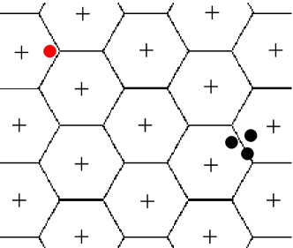
Figure 2: Checking that $\updelta_{s}$ is small, for ${\mathcal{N}}$ the set of crosses (+). Any set $A$ of points close to each other, such as the black dots ($\bullet$), would be ${\mathcal{N}}$-packed (pick $\bm{x}=\bm{c}(A)$ in this case), but would fail to be ${\mathcal{N}}$-packed if too spread (e.g., red dot ($\bullet$) plus black dots). Segments depict the Voronoi diagram of ${\mathcal{N}}$. Best viewed in color.

The following Theorem uses the definition of neighbouring samples: samples ${\mathcal{A}}$ and ${\mathcal{A}}^{\prime}$ are neighbours, written ${\mathcal{A}}\approx{\mathcal{A}}^{\prime}$, iff they differ by one point. We also define $\mathbb{P}[{\mathcal{C}}|{\mathcal{A}}]$ to be the density of output ${\mathcal{C}}$ given input data ${\mathcal{A}}$.

Theorem 9

Fix $\wp_{t}=\mathrm{Id}$ ($\forall t$) and densities $p_{(\bm{\mu}_{.},\bm{\theta}_{.})}$ having the same support $\Omega$ in $k$-variates++. Suppose there exists $\varrho(R)>0$ such that densities $p_{(\bm{\mu}_{.},\bm{\theta}_{.})}$ satisfy the following pointwise likelihood ratio constraint:

$$\frac{p_{(\bm{\mu}_{\bm{a}^{\prime}},\bm{\theta}_{\bm{a}^{\prime}})}(\bm{x})}{p_{(\bm{\mu}_{\bm{a}},\bm{\theta}_{\bm{a}})}(\bm{x})} \leq \varrho(R)\>\>,\forall{\bm{a}},{\bm{a}^{\prime}}\in{\mathcal{A}},\forall\bm{x}\in\Omega\>\>.$$ (15)

Then, there exists a function $f(.)$ such that, for any $\updelta_{w},\updelta_{s}>0$ such that ${\mathcal{A}}$ is $\updelta_{w}$-spread and $\updelta_{s}$-monotonic, for any ${\mathcal{A}}^{\prime}\approx{\mathcal{A}}$, for any $k>0$ and any ${\mathcal{C}}\subset\Omega$ of size $k$ output by Algorithm $k$-variates++ on whichever of ${\mathcal{A}}$ or ${\mathcal{A}}^{\prime}$, the likelihood ratio of ${\mathcal{C}}$ given ${\mathcal{A}}$ and ${\mathcal{A}}^{\prime}$ is upperbounded as:

$$\frac{\mathbb{P}[{\mathcal{C}}|{\mathcal{A}}^{\prime}]}{\mathbb{P}[{\mathcal{C}}|{\mathcal{A}}]} \leq (1+\updelta_{w})^{k-1}+f(k)\cdot\updelta_{w}\cdot\left(1+\updelta_{s}\right)^{k-1}\cdot\varrho(R)\>\>.$$ (16)

(Proof in page Proof of Theorem 9) Notice that Theorem 9 makes just one assumption (15) about the densities, so it can be applied in fairly general settings, such as for regular exponential families (Banerjee et al., 2005). These are a key choice because they extensively cover the domain of distortions for which the average is the population minimiser.

An (almost) distribution-free $1+o(1)$ likelihood ratio

We now show that if ${\mathcal{A}}$ is sampled i.i.d. from any distribution ${\mathcal{D}}$ which satisfies the mild assumption that it is locally bounded everywhere (or almost surely) in a ball, then with high probability the right-hand side of ineq. (16) is $1+o(1)$ where the little-oh vanishes with $m$. The proof, of independent interest, involves an explicit bound on $\updelta_{w}$ and $\updelta_{s}$.

Theorem 10

Suppose ${\mathcal{A}}$ with $|{\mathcal{A}}|=m>1$ sampled i.i.d. from distribution ${\mathcal{D}}$ whose support contains a $L_{2}$ ball $\mathscr{B}_{2}(\bm{0},R)$ with density inside in between $\upepsilon_{m}>0$ and $\upepsilon_{M}\geq\upepsilon_{m}$. Let $\uprho_{{\tiny\mbox{$\mathcal{D}$}}}\stackrel{{\scriptstyle\mathrm{.}}}{{=}}\upepsilon_{M}/\upepsilon_{m}$ ($\geq 1$). For any $0<\updelta<1/2$, if (i) ${\mathcal{A}}\subset\mathscr{B}(\bm{0},R)$ and (ii) the number of clusters $k$ meets:

$$k \leq \frac{\updelta^{2}}{4\uprho_{{\tiny\mbox{$\mathcal{D}$}}}}\cdot\sqrt{m}\>\>,$$ (17)

then there is probability $1-\updelta$ over the sampling of ${\mathcal{A}}$ that $k$-variates++, instantiated as in Theorem 9, satisfies $\mathbb{P}[{\mathcal{C}}|{\mathcal{A}}^{\prime}]/\mathbb{P}[{\mathcal{C}}|{\mathcal{A}}]\leq 1+\uprho_{{\tiny\mbox{$\mathcal{D}$}}}^{k}\cdot g(m,k,d,R)$, $\forall{\mathcal{A}}^{\prime}\approx{\mathcal{A}}$, with

$$g(m,k,d,R) \stackrel{{\scriptstyle\mathrm{.}}}{{=}} \frac{4}{m^{\frac{1}{4}+\frac{1}{d+1}}}+\left(\frac{64}{k^{\frac{2}{d}}}\right)^{k}\cdot\frac{\varrho(2R)}{m}\>\>.$$ (18)

(Proof in page Proof of Theorem 10) The key informal statement of Theorem 10 is that one may obtain with high probability some “good” datasets ${\mathcal{A}}$, i.e., for which $\updelta_{w},\updelta_{s}$ are small, under very weak assumptions about the domain at hand. The key point is that if one has access to the sampling, then one can resample datasets ${\mathcal{A}}$ until a good one comes.

Applications to differential privacy

Let $\mathscr{M}$ be any algorithm which takes as input ${\mathcal{A}}$ and $k$, and returns a set of $k$ centers ${\mathcal{C}}$. Let $\mathbb{P}_{\mathscr{M}}[{\mathcal{C}}|{\mathcal{A}}]$ denote the probability, over the internal randomisation of $\mathscr{M}$, that $\mathscr{M}$ returns ${\mathcal{C}}$ given ${\mathcal{A}}$ and $k$ ($k$, fixed, is omitted in notations). Following is the definition of differential privacy (Dwork et al., 2006), tailored for conciseness to our clustering problem.

Definition 11

$\mathscr{M}$ is $\epsilon$-differentially private (dp) for $k$ clusters iff for any neighbors ${\mathcal{A}}\approx{\mathcal{A}}^{\prime}$, set ${\mathcal{C}}$ of $k$ centers,

$$\mathbb{P}_{\mathscr{M}}[{\mathcal{C}}|{\mathcal{A}}^{\prime}]/\mathbb{P}_{\mathscr{M}}[{\mathcal{C}}|{\mathcal{A}}] \leq \exp\epsilon\>\>.$$ (19)

A relaxed version of $\epsilon$-dp is $(\epsilon,\delta)$-dp, in which we require $\mathbb{P}_{\mathscr{M}}[{\mathcal{C}}|{\mathcal{A}}^{\prime}]\leq\mathbb{P}_{\mathscr{M}}[{\mathcal{C}}|{\mathcal{A}}]\cdot\exp\epsilon+\delta$; thus, $\epsilon$-dp $=(\epsilon,0)$-dp (Dwork & Roth, 2014). We show that low noise may be affordable to satisfy ineq. (19) using Laplace distribution, $Lap(\sigma/\sqrt{2})$. We refer to the Laplace mechanism as a popular mechanism which adds to the output of an algorithm a sufficiently large amount of Laplace noise to be $\epsilon$-dp. We refer to (Dwork et al., 2006) for details, and assume from now on that data belong to a $L_{1}$ ball ${\mathscr{B}}_{1}(\bm{0},R)$.

Theorem 12

Using notations and setting of Theorem 9, let

$$\tilde{\epsilon} \stackrel{{\scriptstyle\mathrm{.}}}{{=}} \log\left(\frac{\exp(\epsilon)-(1+\updelta_{w})^{k-1}}{f(k)\cdot\updelta_{w}\cdot\left(1+\updelta_{s}\right)^{k-1}}\right)\>\>.$$ (20)

Then, $k$-variates++ with $p_{(\bm{\mu}_{.},\bm{\theta}_{.})}$ a product of $Lap(\sigma_{1}/\sqrt{2})$, for $\sigma_{1}\stackrel{{\scriptstyle\mathrm{.}}}{{=}}2\sqrt{2}R/\tilde{\epsilon}$, both meets ineq. (19) and its expected potential satisfies ineq. (7) with

$$\Phi = \Phi_{1}\stackrel{{\scriptstyle\mathrm{.}}}{{=}}8\cdot\left(\phi_{{\tiny\mathrm{opt}}}+\frac{mR^{2}}{\tilde{\epsilon}^{2}}\right)\>\>.$$ (21)

On the other hand, if we opt for $\sigma_{2}\stackrel{{\scriptstyle\mathrm{.}}}{{=}}2\sqrt{2}kR/\epsilon$, then $k$-variates++ is an instance of the Laplace mechanism and its expected potential satisfies ineq. (7) with

$$\Phi = \Phi_{2}\stackrel{{\scriptstyle\mathrm{.}}}{{=}}8\cdot\left(\phi_{{\tiny\mathrm{opt}}}+\frac{mk^{2}R^{2}}{\epsilon^{2}}\right)\>\>.$$ (22)

(Proof in page Proof of Theorem 12) A question is how do $\sigma_{1}$ (resp. $\Phi_{1}$) and $\sigma_{2}$ (resp. $\Phi_{2}$) compare with each other, and how do they compare to the state of the art (Nissim et al., 2007; Wang et al., 2015) (we only consider methods with provable approximation bounds of the global optimum). The key fact is that, if $m$ is sufficiently large, then it happens that we can fix $\updelta_{w}=O(1/m)$ and $\updelta_{s}=O(1)$. The proof of Theorem 10 (page Proof of Theorem 10) and the experiments (page 9) display that such regimes are indeed observed. In this case, it is not hard to show that $\tilde{\epsilon}=\Omega(\epsilon+\log m)$, granting $\sigma_{1}=o(\sigma_{2})$ since

$$\sigma_{1} = O\left(\frac{R}{\epsilon+\log(m)}\right)\>\>,$$ (23)

i.e. the noise guaranteeing ineq. (19) vanishes at $1/\log(m)$ rate. Consequently, in this regime, $\Phi_{1}$ in eq. (21) becomes:

$$\Phi_{1} = \tilde{O}\left(\phi_{{\tiny\mathrm{opt}}}+\frac{mR^{2}}{\left(\epsilon+\log m\right)^{2}}\right)\>\>,$$ (24)

ignoring all factors other than those noted. Thus, the noise dependence grows sublinearly in $m$. Since in this setting, unless all datapoints are the same, $\updelta_{w}$ and $\updelta_{s}$ for ${\mathcal{A}}$ and any possible neighbor ${\mathcal{A}}^{\prime}$ are within $1+o(1)$, it is also possible to overestimate $\updelta_{w}$ and $\updelta_{s}$ to still have $\updelta_{w}=O(1/m)$ and $\updelta_{s}=O(1)$ and grant $\epsilon$-dp for $k$-variates++. Otherwise, the setting of Theorem 10 can be used to grant $(\epsilon,\updelta)$-dp without any tweak. Table 1 compares $k$-variates++ to (Nissim et al., 2007; Wang et al., 2015) in this large sample regime, which is actually a prerequisite for (Nissim et al., 2007; Wang et al., 2015). Notation $O^{*}$ removes all dependencies in their model parameters (assumptions, model parameters, and $\delta$ for the $(\epsilon,\delta)$-dp in (Wang et al., 2015)), and $\uplambda$ is the separability assumption parameter (Nissim et al., 2007). The approximation bounds in (Nissim et al., 2007) consider Wasserstein distance between (estimated / optimal) centers, and not the potential involving data points like us. To obtain bounds that can be compared, we have used the simple trick that the observed potential is, up to a constant, no more than the optimal potential plus a fonction of the distance between (estimated / optimal) centers. This somewhat degrades the bound, but not enough for the observed discrepancies with our bound to reverse or even vanish. It is clear from the bounds that the noise dependence is significantly in our favor, and our bound is also significantly better at least when $k$ is not too large.

5 Experiments

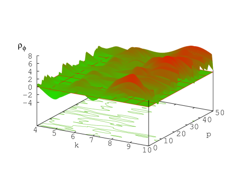
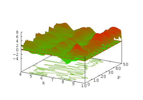
Figure 3: Plot of $\uprho_{\phi}({\mathcal{H}})=f(k,p)$ (points below $z=0$ — isocontour shown — correspond to superior performances for d$k$-means++). Left: ${\mathcal{H}}$=$k$-means++; right: ${\mathcal{H}}$=$k$-means${}_{\tiny{\mbox{$\|$}}}$ (best viewed in color).

The experiments carried out are provided in extenso in the Appendix (from page 9).

d$k$-means++ vs $k$-means++ and $k$-means${}_{\tiny{\mbox{$\|$}}}$ (Bahmani et al., 2012) To address algorithms that can be reduced from $k$-variates++ (Section 3), we have tested d$k$-means++ vs state of the art approach $k$-means${}_{\tiny{\mbox{$\|$}}}$; to be fair with d$k$-means++, we use $k$-means++ seeding as the reclustering algorithm in $k$-means${}_{\tiny{\mbox{$\|$}}}$. Parameters are in line with (Bahmani et al., 2012). To control the spread of Forgy nodes $\phi_{s}^{F}$ (Theorem 4), each peer’s initial data consists of points uniformly sampled in a random hyperrectangle in a space of $d=50$ (expected number of peers points $m_{i}=500,\forall i$). We sample peers until a total of $m\approx$ 20000 point is sampled. Then, each point moves with $p\%$ chances to a uniformly sampled peer. We checked that $\phi_{s}^{F}$ blows up with $p$, i.e., $>$20 times for $p=50\%$ with respect to $p=0$. A remarkable phenomenon was the fact that, even when the number of peers $n$ is quite large (dozens on average), d$k$-means++ is able to beat both $k$-means++ and $k$-means${}_{\tiny{\mbox{$\|$}}}$, even for large values of $p$, as computed by ratio $\uprho_{\phi}({\mathcal{H}})\stackrel{{\scriptstyle\mathrm{.}}}{{=}}100\cdot(\phi(\mbox{{d}$k$-means++})-\phi({\mathcal{H}}))/\phi({\mathcal{H}})$ for ${\mathcal{H}}\in\{k\mbox{-means++},\mbox{$k$-means${}_{\tiny{\mbox{$\|$}}}$}\}$ (Figure 3). Another positive point is that the amount of data to compute a center for d$k$-means++ is in average $\approx n$ times smaller than $k$-means${}_{\tiny{\mbox{$\|$}}}$.

The fact that d$k$-means++, which locally implements the biased seeding, may be able to beat $k$-means++, which globally implements this seeding technique, is not surprising, and in fact may come from the leverage brought by the compartmentalization of distributed data: as discussed in deeper details in page 9, this may even improve the approximability ratio of d$k$-means++ so that it beats the AV bound.

$k$-variates++ vs Forgy-dp and GUPT To address algorithms that can be obtained via a direct use of $k$-variates++ (Section 4), we have tested it in a differential privacy framework vs state of the art approach GUPT (Mohan et al., 2012). We let $\epsilon=1$ in our experiments. We also compare it to Forgy dp (F-dp), which is just Forgy initialisation in the Laplace mechanism, with noise rate (standard dev.) $\propto kR/\epsilon$. In comparison, the noise rate for GUPT is $\propto kR/(\ell\epsilon)$ at the end of its aggregation process, where $\ell$ is the number of blocks. Table 2 gives results for the average (over the choices of $k$) parameters used, $k$, $\overline{\tilde{\epsilon}}$, and ratio $\overline{\uprho^{\prime}_{\phi}}$ where $\uprho^{\prime}_{\phi}({\mathcal{H}})\stackrel{{\scriptstyle\mathrm{.}}}{{=}}\phi({\mathcal{H}})/\phi(\mbox{$k$-variates++})$ — values above 1 indicate better results for $k$-variates++. We use $\tilde{\epsilon}$ as the equivalent $\epsilon$ for $k$-variates++, i.e. the value that guarantees ineq. (19). From Theorem 12, when $\tilde{\epsilon}>\epsilon$, this brings a smaller noise magnitude, desirable for clustering. The obtained results show that $k$-variates++ becomes more of a contender with increasing $m$, but its relative performance tends to decrease with increasing $k$. This is in accordance with the “good” regime of Theorem 12. Results on synthetic domains display the same patterns, along with the fact that relative performances of $k$-variates++ improves with $d$, making it a relevant choice for ”big” domains.

In fact, extensive experiments on synthetic data (page 9) show that intuitions regarding the sublinear noise regime in eq. (24) are experimentally observed, and furthermore they may happen for quite small values of $m$.

Dataset	$m$	$d$	$\overline{k}$	$\overline{(\tilde{\epsilon}/\epsilon)}$	$\overline{\uprho^{\prime}_{\phi}(\mbox{F-{dp}})}$	$\overline{\uprho^{\prime}_{\phi}(\mbox{GUPT})}$
LifeSci	26 733	10	3	4.5	163.0	0.7
Image	34 112	3	2.5	7.9	188.5	2.9
EuropeDiff	169 308	2	5	13.0	2857.1	40.4

Table 2: $k$-variates++ vs F-dp and GUPT (see text).

6 Discussion and Conclusion

We first show in this paper that the $k$-means++ analysis of Arthur and Vassilvitskii can be carried out on a significantly more general scale, aggregating various clustering frameworks of interest and for which no trivial adaptation of $k$-means++ was previously known. Our contributions stand at two levels: (i) we provide the “meta” algorithm, $k$-variates++, and two key results, one on its approximation abilities of the global optimum, and one on the likelihood ratio of the centers it delivers. We do expect further applications of these results, in particular to address several other key clustering problems: stability, generalisation and smoothed analysis (Arthur et al., 2011; von Luxburg, 2010); (ii) we provide two examples of application. The first is a reduction technique from $k$-variates++, which shows a way to obtain straight approximabilty results for other clustering algorithms, some being efficient proxies for the generalisation of existing approaches (Ailon et al., 2009). The second is a direct application of $k$-variates++ to differential privacy, exhibiting a noise component significantly better than existing approaches (Nissim et al., 2007; Wang et al., 2015).

We have not discussed here the possibility to replace the $L_{2}^{2}$ distortion which computes the potential by elements from large and interesting classes — clustering being a huge practical problem, it is indeed reasonable to tailor the distortion to the application at hand. One example are Bregman divergences, that fail simple metric transforms (Acharyya et al., 2013). Another example are total divergences, that fail the simple computation of the population minimizers (Nock et al., 2016; Liu et al., 2012). Some do not even admit population minimizers in closed form (Nielsen & Nock, 2015). It turns out that $k$-variates++, and its good approximation properties, can be extended to such cases (see page Extension to non-metric spaces) for total Jensen divergence (Nielsen & Nock, 2015).

7 Acknowledgments

Thanks are due to Stephen Hardy, Guillaume Smith, Wilko Henecka and Max Ott for stimulating discussions and feedback on the subject. Nicta is funded by the Australian Government through the Department of Communications and the Australian Research Council through the ICT Center of Excellence Program.

Appendix — Table of contents

Appendix on proofs Pg 8
Proof of Theorem 2Pg Proof of Theorem 2
Proof of Lemma 3Pg Proof of Lemma 3
Comments on Table 1Pg Comments on Table 1
Proofs of Theorems 4, 5 and 6Pg Proofs of Theorems 4, 5 and 6
$\hookrightarrow$ Proof of Theorem 4Pg Proof of Theorem 4
$\hookrightarrow$ Proof of Theorem 5Pg Proof of Theorem 5
$\hookrightarrow$ Proof of Theorem 6Pg Proof of Theorem 6
Proof of Theorem 9Pg Proof of Theorem 9
Proof of Theorem 10Pg Proof of Theorem 10
Proof of Theorem 12Pg Proof of Theorem 12
Extension to non-metric spacesPg Extension to non-metric spaces

Appendix on experiments Pg 9
Experiments on Theorem 12 and the sublinear noise regimePg 9
Experiments with d$k$-means++, $k$-means++ and $k$-means${}_{\tiny{\mbox{$\|$}}}$Pg 9
Experiments with $k$-variates++ and GUPTPg 9

8 Appendix on Proofs

Several proofs rely on properties of the $k$-means++ algorithm that are not exploited in the proof of (Arthur & Vassilvitskii, 2007). We assume here the basic knowledge of the proof technique of (Arthur & Vassilvitskii, 2007).

Proof of Theorem 2

Let $A$ denote a subset of ${\mathcal{A}}$, and $\bm{c}(A)\stackrel{{\scriptstyle\mathrm{.}}}{{=}}(1/|A|)\cdot\sum_{\bm{a}\in A}\bm{a}$ the barycenter of $A$. It is well known that $\bm{c}(A)=\arg\min_{\bm{a}^{\prime}\in{\mathbb{R}}^{d}}\sum_{\bm{a}\in A}\|\bm{a}-\bm{a}^{\prime}\|_{2}^{2}$, so the potential of $A$,

$$\phi(A) \stackrel{{\scriptstyle\mathrm{.}}}{{=}} \sum_{\bm{a}\in A}\|\bm{a}-\bm{c}(A)\|_{2}^{2}$$ (25)

is just the optimal potential of $A$ if $A$ defines a cluster in the optimal clustering. We also define the noisy potential of $A$ as:

$$\phi^{N}(A) \stackrel{{\scriptstyle\mathrm{.}}}{{=}} \sum_{\bm{a}\in A}\int_{\Omega_{\bm{a}}}\|\bm{x}-\bm{c}(A)\|_{2}^{2}\mathrm{d}p_{\bm{a}}(\bm{x})\>\>.$$ (26)

The proof of Theorem 2 follows the same path as the proof of Theorem 3.1 in (Arthur & Vassilvitskii, 2007). Instead of reproducing the proof, we shall assume basic knowledge of the original proof and will just provide the side Lemmata that are sufficient for our more general result. The first Lemma is a generalization of Lemma 3.2 in (Arthur & Vassilvitskii, 2007).

Lemma 13

Let $C_{{\tiny\mathrm{opt}}}$ denotes the optimal partition of ${\mathcal{A}}$ according to eq. (2). Let $A$ be an arbitrary cluster in $C_{{\tiny\mathrm{opt}}}$. Let $C$ be a single-cluster clustering whose center is chosen at random by one step of Algorithm $k$-variates++ (i.e. for $t=1$). Then

$$\mathbb{E}[\phi(A)] = \phi_{\mathrm{{\tiny\mathrm{opt}}}}(A)+\phi^{N}_{\mathrm{{\tiny\mathrm{opt}}}}(A)\>\>.$$ (27)

Proof.

The expected potential of cluster $A$ is

$$\mathbb{E}[\phi(A;{\mathcal{C}}=\emptyset)]$$ (30)

$$= \frac{1}{|A|}\cdot\sum_{\bm{a}_{0}\in A}\int_{\Omega_{{\bm{a}}_{0}}}\sum_{\bm{a}\in A}\|\bm{a}-\bm{x}\|_{2}^{2}\mathrm{d}p_{\bm{a}_{0}}(\bm{x})$$

$$= \frac{1}{|A|}\cdot\sum_{\bm{a}_{0}\in A}\int_{\Omega_{{\bm{a}}_{0}}}\sum_{\bm{a}\in A}\|\bm{a}-\bm{c}(A)+\bm{c}(A)-\bm{x}\|_{2}^{2}\mathrm{d}p_{\bm{a}_{0}}(\bm{x})$$

$$= \frac{1}{|A|}\cdot\sum_{\bm{a}_{0}\in A}\left(\begin{array}[]{l}\sum_{\bm{a}\in A}\|\bm{a}-\bm{c}(A)\|_{2}^{2}+|A|\cdot\int_{\Omega_{{\bm{a}}_{0}}}\|\bm{x}-\bm{c}(A)\|_{2}^{2}\mathrm{d}p_{\bm{a}_{0}}(\bm{x})\\ +2\sum_{\bm{a}\in A}\langle\bm{a}-\bm{c}(A),\bm{c}(A)-\int_{\Omega_{{\bm{a}}_{0}}}\bm{x}\mathrm{d}p_{\bm{a}_{0}}(\bm{x})\rangle\end{array}\right)$$

$$= \frac{1}{|A|}\cdot\sum_{\bm{a}_{0}\in A}\left(\begin{array}[]{l}\sum_{\bm{a}\in A}\|\bm{a}-\bm{c}(A)\|_{2}^{2}\par+|A|\cdot\int_{\Omega_{{\bm{a}}_{0}}}\|\bm{x}-\bm{c}(A)\|_{2}^{2}\mathrm{d}p_{\bm{a}_{0}}(\bm{x})\\ +2\langle\underbrace{\sum_{\bm{a}\in A}\bm{a}-|A|\bm{c}(A)}_{=0},\bm{c}(A)-\bm{a}_{0}\rangle\end{array}\right)$$

$$= \sum_{\bm{a}\in A}\|\bm{a}-\bm{c}(A)\|_{2}^{2}+\sum_{\bm{a}\in A}\int_{\Omega_{{\bm{a}}_{0}}}\|\bm{x}-\bm{c}(A)\|_{2}^{2}\mathrm{d}p_{\bm{a}}(\bm{x})$$

$$= \phi_{\mathrm{{\tiny\mathrm{opt}}}}(A)+\phi^{N}_{\mathrm{{\tiny\mathrm{opt}}}}(A)\>\>,$$

as claimed. ∎

When $p_{\bm{a}}$ is a Dirac anchored at $\bm{a}$, we recover Lemma 3.2 in (Arthur & Vassilvitskii, 2007). The following Lemma generalizes Lemma 3.3 in (Arthur & Vassilvitskii, 2007).

Lemma 14

Suppose that the optimal clustering $C_{{\tiny\mathrm{opt}}}$ is $\upeta$-probe approximable. Let $A$ be an arbitrary cluster in $C_{{\tiny\mathrm{opt}}}$, and let $C$ be an arbitrary clustering with centers ${\mathcal{C}}$. Suppose that the reference point $\bm{a}$ chosen according to (1) in Step 2.1 is in $A$. Then the random point $\bm{x}$ picked in Step 2.2 brings an expected potential that satisfies

$$\mathbb{E}[\phi(A)] \leq (6+4\upeta)\cdot\phi_{{\tiny\mathrm{opt}}}(A)+2\cdot\phi^{N}_{\mathrm{{\tiny\mathrm{opt}}}}(A)\>\>.$$ (34)

Proof.

Let us denote ${\bm{c}}^{\star}(\bm{u})\stackrel{{\scriptstyle\mathrm{.}}}{{=}}\arg\min_{\bm{x}\in{\mathcal{C}}}\|\bm{u}-\bm{x}\|_{2}^{2}$ (since $C\neq C_{{\tiny\mathrm{opt}}}$ in general, ${\bm{c}}^{\star}(\bm{u})\neq{\bm{c}}_{{\tiny\mathrm{opt}}}(\bm{u})$), and $D(\bm{a})\stackrel{{\scriptstyle\mathrm{.}}}{{=}}\|\bm{a}-{\bm{c}}^{\star}(\bm{a})\|_{2}^{2}$ the contribution of $\bm{a}\in A$ to the $k$-means potential defined by ${\mathcal{C}}$. We have, using Lemma 3.3 in (Arthur & Vassilvitskii, 2007) and Lemma 13,

$$\mathbb{E}_{\bm{x}}[\phi(A;{\mathcal{C}}\cup\{\bm{x}\})] = \sum_{\bm{a}_{0}\in A}\frac{D_{t}(\bm{a}_{0})}{\sum_{\bm{a}\in A}D_{t}(\bm{a})}\cdot\sum_{\bm{a}\in A}\int_{\Omega_{{\bm{a}}_{0}}}\min\{D(\bm{a}),\|\bm{a}-\bm{x}\|_{2}^{2}\}\mathrm{d}p_{\bm{a}_{0}}(\bm{x})\>\>.$$ (35)

The triangle inequality gives, for any $\bm{a}\in A$,

$$\sqrt{D_{t}(\bm{a}_{0})} \stackrel{{\scriptstyle\mathrm{.}}}{{=}} \|\wp_{t}(\bm{a}_{0})-{\bm{c}}^{\star}(\wp_{t}(\bm{a}_{0}))\|_{2}$$ (36)

$$\leq \|\wp_{t}(\bm{a}_{0})-{\bm{c}}^{\star}(\wp_{t}(\bm{a}))\|_{2}$$

$$\leq \|\wp_{t}(\bm{a}_{0})-\wp_{t}(\bm{a})\|_{2}+\|\wp_{t}(\bm{a})-{\bm{c}}^{\star}(\wp_{t}(\bm{a}))\|_{2}\>\>;$$

since $(a+b)^{2}\leq 2a^{2}+2b^{2}$, then $D_{t}(\bm{a}_{0})\leq 2\|\wp_{t}(\bm{a}_{0})-\wp_{t}(\bm{a})\|_{2}^{2}+2D_{t}(\bm{a})$, and so, after averaging over $A$,

$$D_{t}(\bm{a}_{0}) \leq \frac{2}{|A|}\sum_{\bm{a}\in A}\|\wp_{t}(\bm{a}_{0})-\wp_{t}(\bm{a})\|_{2}^{2}+\frac{2}{|A|}\sum_{\bm{a}\in A}D_{t}(\bm{a})\>\>,$$ (37)

and eq. (35) can be upperbounded as:

$$\mathbb{E}_{\bm{x}}[\phi(A;{\mathcal{C}}\cup\{\bm{x}\})] \leq \frac{2}{|A|}\sum_{\bm{a}_{0}\in A}\frac{\sum_{\bm{a}\in A}\|\wp_{t}(\bm{a}_{0})-\wp_{t}(\bm{a})\|_{2}^{2}}{\sum_{\bm{a}\in A}D_{t}(\bm{a})}\cdot\sum_{\bm{a}\in A}\int_{\Omega_{{\bm{a}}_{0}}}\min\{D(\bm{a}),\|\bm{a}-\bm{x}\|_{2}^{2}\}\mathrm{d}p_{\bm{a}_{0}}(\bm{x})$$ (38)

$$+\frac{2}{|A|}\sum_{\bm{a}_{0}\in A}\frac{\sum_{\bm{a}\in A}D_{t}(\bm{a})}{\sum_{\bm{a}\in A}D_{t}(\bm{a})}\cdot\sum_{\bm{a}\in A}\int_{\Omega_{{\bm{a}}_{0}}}\min\{D(\bm{a}),\|\bm{a}-\bm{x}\|_{2}^{2}\}\mathrm{d}p_{\bm{a}_{0}}(\bm{x})$$

$$\leq \underbrace{\frac{2}{|A|}\sum_{\bm{a}_{0}\in A}\frac{\sum_{\bm{a}\in A}D(\bm{a})}{\sum_{\bm{a}\in A}D_{t}(\bm{a})}\cdot\sum_{\bm{a}\in A}\|\wp_{t}(\bm{a}_{0})-\wp_{t}(\bm{a})\|_{2}^{2}}_{\stackrel{{\scriptstyle\mathrm{.}}}{{=}}P_{1}}$$

$$+\underbrace{\frac{2}{|A|}\sum_{\bm{a}_{0}\in A}\sum_{\bm{a}\in A}\int_{\Omega_{{\bm{a}}_{0}}}\|\bm{a}-\bm{x}\|_{2}^{2}\mathrm{d}p_{\bm{a}_{0}}(\bm{x})}_{\stackrel{{\scriptstyle\mathrm{.}}}{{=}}P_{2}}\>\>.$$

We bound the two potentials $P_{1}$ and $P_{2}$ separately, starting with $P_{1}$. Fix any $\bm{a}_{0}\in A$. If $\sum_{\bm{a}\in A}\|\wp_{t}(\bm{a})-\wp_{t}(\bm{a}_{0})\|_{2}^{2}=0$, then trivially

$$\left(\sum_{\bm{a}\in A}D(\bm{a})\right)\cdot\left(\sum_{\bm{a}\in A}\|\wp_{t}(\bm{a}_{0})-\wp_{t}(\bm{a})\|_{2}^{2}\right) \leq (1+\upeta)\cdot\left(\sum_{\bm{a}\in A}D_{t}(\bm{a})\right)\cdot\left(\sum_{\bm{a}\in A}\|\bm{a}_{0}-\bm{a}\|_{2}^{2}\right)\>\>,$$ (39)

since the right-hand side cannot be negative. If $\sum_{\bm{a}\in A}\|\wp_{t}(\bm{a})-\wp_{t}(\bm{a}_{0})\|_{2}^{2}\neq 0$, then since $\wp_{t}$ is $\upeta$-stretching, we have:

$$\frac{\sum_{\bm{a}\in A}\|\bm{a}-\bm{c}^{\star}(\bm{a})\|_{2}^{2}}{\sum_{\bm{a}\in A}\|\bm{a}-\bm{a}_{0}\|_{2}^{2}} \leq (1+\upeta)\cdot\frac{\sum_{\bm{a}\in A}\|\wp_{t}(\bm{a})-\bm{c}^{\star}(\wp_{t}(\bm{a}))\|_{2}^{2}}{\sum_{\bm{a}\in A}\|\wp_{t}(\bm{a})-\wp_{t}(\bm{a}_{0})\|_{2}^{2}}\>\>,$$ (40)

which is exactly ineq. (39) after rearranging the terms. Ineq (39) implies

$$P_{1} \leq 2(1+\upeta)\cdot\frac{1}{|A|}\sum_{\bm{a}_{0}\in A}\sum_{\bm{a}\in A}\|\bm{a}_{0}-\bm{a}\|_{2}^{2}$$ (41)

$$=4(1+\upeta)\cdot\phi_{{\tiny\mathrm{opt}}}(A)\>\>,$$

where the equality follows from (Arthur & Vassilvitskii, 2007), Lemma 3.2. Also, Lemma 13 brings

$$P_{2} = 2\cdot\frac{1}{|A|}\sum_{\bm{a}_{0}\in A}\int_{\Omega_{{\bm{a}}_{0}}}\sum_{\bm{a}\in A}\|\bm{a}-\bm{x}\|_{2}^{2}\mathrm{d}p_{\bm{a}_{0}}(\bm{x})$$ (42)

$$= 2\phi_{\mathrm{{\tiny\mathrm{opt}}}}(A)+2\phi^{N}_{\mathrm{{\tiny\mathrm{opt}}}}(A)\>\>.$$

We therefore get

$$\mathbb{E}_{\bm{x}}[\phi(A;{\mathcal{C}}\cup\{\bm{x}\})] \leq (6+4\upeta)\cdot\phi_{{\tiny\mathrm{opt}}}(A)+2\cdot\phi^{N}_{\mathrm{{\tiny\mathrm{opt}}}}(A)\>\>,$$ (43)

as claimed. ∎

Again, we recover Lemma 3.3 in (Arthur & Vassilvitskii, 2007) when $p_{\bm{a}}$ is a Dirac and the probe function $\wp=\mathrm{Id}$. The rest of the proof of Theorem 2 consists of the same steps as Theorem 3.1 in (Arthur & Vassilvitskii, 2007), after having remarked that $\phi^{N}_{\mathrm{{\tiny\mathrm{opt}}}}(A)$ can be simplified:

$$\phi_{{\tiny\mathrm{opt}}}^{N}(A) = \sum_{\bm{a}\in A}\int_{\Omega_{{\bm{a}}_{0}}}\|\bm{x}-\bm{c}(A)\|_{2}^{2}\mathrm{d}p_{\bm{a}}(\bm{x})$$ (44)

$$= \sum_{\bm{a}\in A}\int_{\Omega_{{\bm{a}}_{0}}}\|\bm{x}\|_{2}^{2}\mathrm{d}p_{\bm{a}}(\bm{x})-2\langle\bm{c}(A),\bm{\mu}_{\bm{a}}\rangle+\|\bm{c}(A)\|_{2}^{2}$$

$$= \sum_{\bm{a}\in A}\int_{\Omega_{{\bm{a}}_{0}}}\|\bm{x}-\bm{\mu}_{\bm{a}}\|_{2}^{2}\mathrm{d}p_{\bm{a}}(\bm{x})+\|\bm{\mu}_{\bm{a}}\|_{2}^{2}-2\langle\bm{c}(A),\bm{a}\rangle+\|\bm{c}(A)\|_{2}^{2}$$

$$= \sum_{\bm{a}\in A}\left\{\mathrm{tr}\left(\Sigma_{\bm{a}}\right)+\|\bm{\mu}_{\bm{a}}-\bm{c}(A)\|_{2}^{2}\right\}$$

$$= \phi_{{\tiny\mathrm{bias}}}(A)+\phi_{{\tiny\mathrm{var}}}(A)\>\>.$$

Proof of Lemma 3

The proof is a simple application of the Fréchet-Cramér-Rao-Darmois bound. Consider the simple case $k=1$ and a spherical Gaussian noise for $p$ with a single point in ${\mathcal{A}}$. Renormalize both sides of (7) by $m\stackrel{{\scriptstyle\mathrm{.}}}{{=}}|{\mathcal{A}}|$ so that $(1/m)\sum_{a\in{\mathcal{A}}}\mathrm{tr}\left(\Sigma_{\bm{a}}\right)=\mathrm{tr}\left(\Sigma\right)$. One sees that the left hand side of ineq. (7) is just an estimator of the variance of $p_{\bm{a}}$, which, by Fréchet-Darmois-Cramér-Rao bound, has to be at least the inverse of the Fisher information, that is in this case, the trace of the covariance matrix, i.e. $\mathrm{tr}\left(\Sigma\right)$.

Comments on Table 1

(Wang et al., 2015) are concerned with approximating subspace clustering, and so they are using a very different potential function, which is, between two subspaces ${\mathcal{S}}$ and ${\mathcal{S}}^{\prime}$, $d({\mathcal{S}},{\mathcal{S}}^{\prime})=\|\mbox{{\small{u}}}\mbox{{\small{u}}}^{\top}-\mbox{{\small{u}}}^{\prime}\mbox{{\small{u}}}^{\prime\top}\|_{F}$, where u (resp. $\mbox{{\small{u}}}^{\prime}$) is an orthonormal basis for ${\mathcal{S}}$ (resp. ${\mathcal{S}}^{\prime}$). To obtain an idea of the approximation on the $k$-means clustering problem that their technique yields, we compute $\phi$ in the projected space, using the fact that, because of the triangle inequality and the fact that projections are linear and do not increase norms,

$$\|\mathrm{proj}_{\mbox{{\small{u}}}}(\bm{a})-\mathrm{proj}_{\mbox{{\small{u}}}^{\prime}}(\bm{a}^{\prime})\|_{2} = \|(\mathrm{proj}_{\mbox{{\small{u}}}}(\bm{a})-\mathrm{proj}_{\mbox{{\small{u}}}}(\bm{a}^{\prime}))+(\mathrm{proj}_{\mbox{{\small{u}}}}(\bm{a}^{\prime})-\mathrm{proj}_{\mbox{{\small{u}}}^{\prime}}(\bm{a}^{\prime}))\|_{2}$$ (45)

$$\leq \|\mathrm{proj}_{\mbox{{\small{u}}}}(\bm{a})-\mathrm{proj}_{\mbox{{\small{u}}}}(\bm{a}^{\prime})\|_{2}+\|\mathrm{proj}_{\mbox{{\small{u}}}}(\bm{a}^{\prime})-\mathrm{proj}_{\mbox{{\small{u}}}^{\prime}}(\bm{a}^{\prime}))\|_{2}$$ (46)

$$\leq \|\mathrm{proj}_{\mbox{{\small{u}}}}(\bm{a})-\mathrm{proj}_{\mbox{{\small{u}}}}(\bm{a}^{\prime})\|_{2}+2\|\bm{a}^{\prime}\|_{2}\>\>.$$ (47)

To account for the approximation in the inequalities, we then discard the rightmost term, replacing therefore $\|\mathrm{proj}_{\mbox{{\small{u}}}}(\bm{a})-\mathrm{proj}_{\mbox{{\small{u}}}^{\prime}}(\bm{a}^{\prime})\|_{2}$ by $\|\mathrm{proj}_{\mbox{{\small{u}}}}(\bm{a})-\mathrm{proj}_{\mbox{{\small{u}}}}(\bm{a}^{\prime})\|_{2}$, which amounts, in the approximation bounds, to remove the dependence in the dimension. At this price, and using the trick to transfer the wasserstein distance between centers to $L_{2}^{2}$ potential between points to cluster centers, we obtain the approximation bound in ($\beta$) of Table 1. While it has to be used with care, its main interest is in showing that the price to pay because of the noise component is in fact not decreasing in $m$.

Proofs of Theorems 4, 5 and 6

The proof of these Theorems uses a reduction from $k$-variates++ to the corresponding algorithms, meaning that there exists particular probe functions and densities for which the set of centers delivered by $k$-variates++ is the same as the one delivered by the corresponding algorithms.

Definition 15

Let ${\mathcal{H}}$ (parameters omitted) be any hard membership $k$-clustering algorithm. We way that $k$-variates++ reduces to ${\mathcal{H}}$ iff there exists data, densities and probe functions depending on the instance of ${\mathcal{H}}$ such that, in expectation over the internal randomisation of ${\mathcal{H}}$, the set of centers delivered by ${\mathcal{H}}$ are the same as the ones delivered by $k$-variates++. We note it

$$k \succeq {\mathcal{H}}\>\>.$$-variates++ (48)

Hence, whenever $\mbox{$k$-variates++}\succeq{\mathcal{H}}$, Theorem 2 immediately gives a guarantee for the approximation of the global optimum in expectation for ${\mathcal{H}}$, but this requires the translation of the parameters involved in $\Phi$ in ineq. (7) to involve only parameters from ${\mathcal{H}}$. In all our examples, this translation poses no problem at all.

Proof of Theorem 4

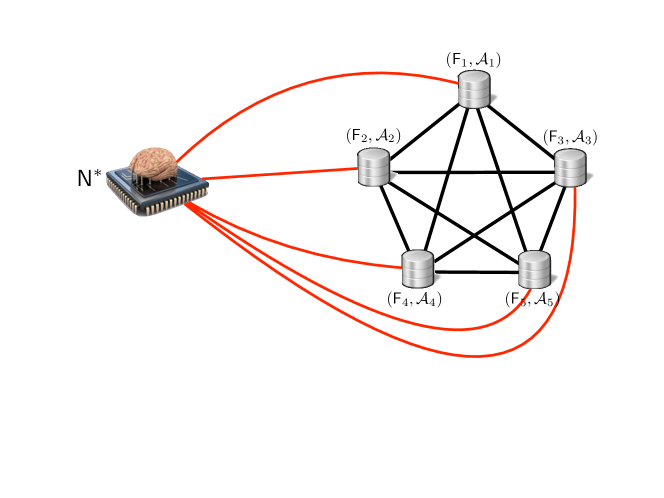
Figure 4: Message passing between peers / nodes in the d$k$-means++/pd$k$-means++ framework. Black edges and red arcs denote message passing between peers / nodes. On each black edge circulates at most $k$ data points; on each red arcs circulates $k$ total potentials.

Figure 4 presents the architecture of message passing in the d$k$-means++/pd$k$-means++ framework. We first focus on the protected scheme, d$k$-means++. We reduce $k$-variates++ to Algorithm 1 using identity probe functions: $\wp_{t}=\mathrm{Id},\forall t$. The trick in reduction relies on the densities. We let $p_{\bm{\mu}_{\bm{a}},\bm{\theta}_{\bm{a}}}$ be uniform over the subset ${\mathcal{A}}_{i}$ to which $\bm{a}$ belongs. Thus, the support of densities is discrete, and ${\mathcal{C}}$ is a subset of ${\mathcal{A}}$; furthermore, the probability $q_{t}(\bm{a})$ that $\bm{a}\in{\mathcal{A}}_{i}$ is chosen at iteration $t$ in $k$-variates++ actually simplifies to a convenient expression:

$$q_{t}(\bm{a}) = q^{D}_{ti}\cdot u_{i}\>\>,$$ (49)

where we recall that

$$q^{D}_{ti} \stackrel{{\scriptstyle\mathrm{.}}}{{=}} \left\{\begin{array}[]{ccl}D_{t}({\mathcal{A}}_{i})\cdot(\sum_{j}D_{t}({\mathcal{A}}_{j}))^{-1}&\mbox{ if }&t>1\\ (1/n)&\lx@intercol\mbox{ otherwise}\hfil\lx@intercol\end{array}\right.\>\>.$$ (52)

Hence, picking $\bm{a}$ can be equivalently done by first picking ${\mathcal{A}}_{i}$ using $q^{D}_{t}$, and then, given the $i$ chosen, sampling uniformly at random $\bm{a}$ in ${\mathcal{A}}_{i}$, which is what Forgy nodes do. We therefore get the equivalence between Algorithm 1 and $k$-variates++ as instantiated.

Lemma 16

With data, densities and probes defined as before, $k$-variates++ $\succeq$ d$k$-means++.

To get the approximability ratio of d$k$-means++, we translate the parameters of $\Phi$ in ineq. (7). First, since $(a+b)^{2}\leq 2a^{2}+2b^{2}$,

$$\phi_{{\tiny\mathrm{bias}}} \stackrel{{\scriptstyle\mathrm{.}}}{{=}} \sum_{\bm{a}\in{\mathcal{A}}}\|\bm{\mu}_{\bm{a}}-\bm{c}_{{\tiny\mathrm{opt}}}(\bm{a})\|_{2}^{2}$$ (54)

$$= \sum_{i\in[n]}\sum_{\bm{a}\in{\mathcal{A}}_{i}}\|\bm{c}({\mathcal{A}}_{i})-\bm{c}_{{\tiny\mathrm{opt}}}(\bm{a})\|_{2}^{2}$$

$$= \sum_{i\in[n]}\sum_{\bm{a}\in{\mathcal{A}}_{i}}\|\bm{c}({\mathcal{A}}_{i})-\bm{a}+\bm{a}-\bm{c}_{{\tiny\mathrm{opt}}}(\bm{a})\|_{2}^{2}$$

$$\leq 2\sum_{i\in[n]}\sum_{\bm{a}\in{\mathcal{A}}_{i}}\|\bm{c}({\mathcal{A}}_{i})-\bm{a}\|_{2}^{2}+2\sum_{\bm{a}\in{\mathcal{A}}}\|\bm{a}-\bm{c}_{{\tiny\mathrm{opt}}}(\bm{a})\|_{2}^{2}$$

$$=2\phi^{F}_{s}+2\phi_{{\tiny\mathrm{opt}}}\>\>.$$

Furthermore,

$$\phi_{{\tiny\mathrm{var}}} \stackrel{{\scriptstyle\mathrm{.}}}{{=}} \sum_{\bm{a}\in{\mathcal{A}}}\mathrm{tr}\left(\Sigma_{\bm{a}}\right)$$ (55)

$$= \sum_{\bm{a}\in{\mathcal{A}}}\int_{\Omega_{\bm{a}}}\|\bm{x}-\bm{\mu}_{\bm{a}}\|_{2}^{2}\mathrm{d}p_{\bm{a}}(\bm{x})$$

$$= \sum_{i\in[n]}\sum_{\bm{a}\in{\mathcal{A}}_{i}}\sum_{\bm{a}^{\prime}\in{\mathcal{A}}_{i}}\frac{1}{m_{i}}\cdot\|\bm{a}^{\prime}-\bm{c}({\mathcal{A}}_{i})\|_{2}^{2}$$

$$= \sum_{i\in[n]}\sum_{\bm{a}\in{\mathcal{A}}_{i}}\|\bm{a}-\bm{c}({\mathcal{A}}_{i})\|_{2}^{2}=\phi^{F}_{s}\>\>.$$

There remains to plug ineq. (54) and eq. (55) in Theorem 2, along with $\upeta=0$ (since $\wp=\mathrm{Id}$), to get $\mathbb{E}[\phi({\mathcal{A}};{\mathcal{C}})]\leq(2+\log k)\cdot\left(10\phi_{{\tiny\mathrm{opt}}}+6\phi_{s}\right)$, as in Theorem 4.

The private version, pd$k$-means++, follows immediately by leaving $\phi_{{\tiny\mathrm{var}}}$ in $\Phi$ instead of carrying eq. (55). This ends the proof of Theorem 4.

Proof of Theorem 5

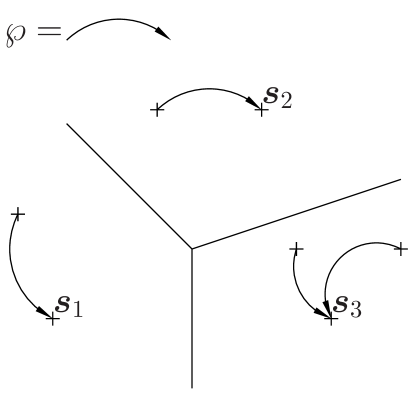
Figure 5: Computation of the probe function $\wp$ for the reduction from $k$-variates++ to s$k$-means++. Segments display parts of the Voronoi diagram of ${\mathcal{S}}$.

The proof proceeds in the same way as for Theorem 4. The probe function (the same for every iteration, $\wp_{t}=\wp,\forall t$) is already defined in the statement of Theorem 5, from the definition of synopses. The distributions $p_{\bm{\mu}_{\bm{a}},\bm{\theta}_{\bm{a}}}$ are Diracs anchored at the probe (synopses) locations. The centers chosen in $k$-variates++ are thus synopses, and it is not hard to check that the probability to pick a synopsis $\bm{s}_{j}$ at iteration $t$ factors in the same way as in the definition of $q^{S}_{t}$ in eq. (11). We therefore get the equivalence between Algorithm 2 and $k$-variates++ as instantiated.

Lemma 17

With data, densities and probes defined as before, $k$-variates++ $\succeq$ s$k$-means++.

The proof of the approximation property of s$k$-means++ then follows from the fact that $\phi_{{\tiny\mathrm{var}}}=0$ (Diracs) and

$$\phi_{{\tiny\mathrm{bias}}} \stackrel{{\scriptstyle\mathrm{.}}}{{=}} \sum_{\bm{a}\in{\mathcal{A}}}\|\bm{\mu}_{\bm{a}}-\bm{c}_{{\tiny\mathrm{opt}}}(\bm{a})\|_{2}^{2}$$ (56)

$$= \sum_{\bm{a}\in{\mathcal{A}}}\|\wp({\bm{a}})-\bm{c}_{{\tiny\mathrm{opt}}}(\bm{a})\|_{2}^{2}$$

$$= \sum_{\bm{a}\in{\mathcal{A}}}\|\wp({\bm{a}})-{\bm{a}}+{\bm{a}}-\bm{c}_{{\tiny\mathrm{opt}}}(\bm{a})\|_{2}^{2}$$

$$\leq 2\sum_{\bm{a}\in{\mathcal{A}}}\|\wp({\bm{a}})-{\bm{a}}\|_{2}^{2}+2\sum_{\bm{a}\in{\mathcal{A}}}\|{\bm{a}}-\bm{c}_{{\tiny\mathrm{opt}}}(\bm{a})\|_{2}^{2}$$

$$=2\sum_{\bm{a}\in\mathsf{S}}\|\wp({\bm{a}})-{\bm{a}}\|_{2}^{2}+2\sum_{\bm{a}\in\mathsf{S}}\|{\bm{a}}-\bm{c}_{{\tiny\mathrm{opt}}}(\bm{a})\|_{2}^{2}=2\phi^{\wp}_{s}+2\phi_{{\tiny\mathrm{opt}}}$$

(using again $(a+b)^{2}\leq 2a^{2}+2b^{2}$). Using Theorem 2, this brings the statement of the Theorem.

Figure 5 shows that the ”quality” of the probe function (spread $\phi^{\wp}_{s}$, stretching factor $\upeta$) stem from the quality of the Voronoi diagram induced by the synopses in ${\mathcal{S}}$.

Proof of Theorem 6

Setting	Algorithm	Probe functions $\wp_{t}$	Densities $p_{(\bm{\mu}_{.},\bm{\theta}_{.})}$
Batch	$k$-means++ (Arthur & Vassilvitskii, 2007)	Identity	Diracs
Distributed	d$k$-means++	Identity	Uniform on data subsets
Distributed	pd$k$-means++	Identity	Non uniform, compact support
Streaming	s$k$-means++	synopses	Diracs
On-line	ol$k$-means++	point (batch not hit)	Diracs
		/ closest center (batch hit)

Table 3: Synthesis of the parameters for the reductions from $k$-variates++. We indicate $k$-means++ as the batch clustering solution (Arthur & Vassilvitskii, 2007).

The proof proceeds in the same way as for Theorem 4. The the reduction from $k$-variates++ to ol$k$-means++ relies on two things: first, the uniform choice of the first center in $k$-means++ can be replaced by picking the center uniformly in any subset of the data: it does not change the expected approximation properties of the algorithm (this comes from Lemma 3.4 in (Arthur & Vassilvitskii, 2007)); therefore, the choice $q_{1}\stackrel{{\scriptstyle\mathrm{.}}}{{=}}u_{m}$ in $k$-variates++ can be replaced with $q_{1}\stackrel{{\scriptstyle\mathrm{.}}}{{=}}u_{1}$ (uniform with support ${\mathcal{A}}_{1}$). Second, a particular probe function needs to be devised, sketched in Figure 6. Basically, all probe functions of a minibatch are the same: each point in the minibatch is probed to itself, while points occurring outside the minibatch are probed to their closest center. The reduction proceeds in the following steps: we first let ${\mathcal{A}}$ be the complete set of points in the stream $\mathsf{S}$. Then, we let ${\mathcal{A}}_{j}$ denote the set of points of minibatch $\mathsf{S}_{j}$. Remark that minibatch ${\mathcal{A}}_{j}$ occurs in the stream before ${\mathcal{A}}_{j^{\prime}}$ for $j<j^{\prime}$, and minibatches induce a partition of ${\mathcal{A}}$. Let $j(t)$ denote the batch related to iteration $t$ in $k$-variates++. We define the following probe function $\wp_{t}(\bm{a})$ in $k$-variates++, letting ${\mathcal{A}}_{j}$ the minibatch to which $\bm{a}$ belongs (we do not necessarily have $j=j(t)$):

• if $j=j(t)$, then $\wp_{t}(\bm{a})\stackrel{{\scriptstyle\mathrm{.}}}{{=}}\bm{a}$;

• else $\wp_{t}(\bm{a})\stackrel{{\scriptstyle\mathrm{.}}}{{=}}\arg\min_{\bm{c}\in{\mathcal{C}}}\|\bm{a}-\bm{c}\|_{2}^{2}$ (remark that $|{\mathcal{C}}|\geq 1$ in this case).

Finally, densities $p_{(\bm{\mu}_{.},\bm{\theta}_{.})}$ are Diracs anchored at selected points, like in $k$-means++. We get the equivalence between Algorithm 3 and $k$-variates++ as instantiated.

Lemma 18

With data, densities and probes defined as before, $k$-variates++ $\succeq$ ol$k$-means++.

The proof is immediate, since each minibatch is hit by a center exactly once in ol$k$-means++, and when one subset ${\mathcal{A}}_{j}$ is hit by a center, then the probe function makes that no other center can be sampled again from ${\mathcal{A}}_{j}$ (all contributions to the density $q_{t}$ are then zero in ${\mathcal{A}}_{j}$). We now finish the proof of Theorem 6 by showing the same approximability ratio for $k$-variates++ as reduced.

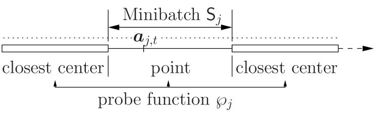
Figure 6: Computation of the probe function $\wp_{t}$ for the reduction from ol$k$-means++ to $k$-variates++, depending on each minibatch stream $\mathsf{S}_{j}$.

Because optimal clusters are $\varsigma$-wide with respect to stream $\mathsf{S}$, we have

$$\frac{1}{|A|}\cdot\sum_{\bm{a},\bm{a}^{\prime}\in A}\|\bm{a}-\bm{a}^{\prime}\|_{2}^{2} \geq \varsigma\cdot R\>\>.$$

Recall that $\bm{c}(A)\stackrel{{\scriptstyle\mathrm{.}}}{{=}}(1/|A|)\cdot\sum_{\bm{a}\in A}\bm{a}$. For any $\bm{a}_{0}\in A$, it holds that:

$$\frac{1}{|A|-1}\cdot\sum_{\bm{a}\in A}\|\bm{a}-\bm{a}_{0}\|_{2}^{2} \geq \frac{1}{|A|-1}\cdot\sum_{\bm{a}\in A}\|\bm{a}-\bm{c}(A)\|_{2}^{2}$$

$$=\frac{1}{|A|-1}\cdot\left(\frac{1}{2|A|}\cdot\sum_{\bm{a},\bm{a}^{\prime}\in A}\|\bm{a}-\bm{a}^{\prime}\|_{2}^{2}\right)$$

$$= \frac{1}{4}\cdot\frac{2}{|A|(|A|-1)}\cdot\sum_{\bm{a},\bm{a}^{\prime}\in A}\|\bm{a}-\bm{a}^{\prime}\|_{2}^{2}$$

$$\geq \frac{\varsigma}{4}\cdot R\>\>.$$ (59)

Ineq. (Proof of Theorem 6) holds because $\bm{c}(A)$ is the population minimizer for optimal cluster $A$ (see e.g., (Arthur & Vassilvitskii, 2007), Lemma 2.1). Since probes are points of ${\mathcal{A}}$,

$$\phi(\wp_{j}(A);\{\wp_{j}(\bm{a}_{0})\}) \leq |A|\cdot R$$ (60)

$$\leq \frac{4|A|}{\varsigma(|A|-1)}\cdot\sum_{\bm{a}\in A}\|\bm{a}-\bm{a}_{0}\|_{2}^{2}\>\>.$$

On the other hand, we have:

$$\phi(\wp_{t}(A);{\mathcal{C}}) = \sum_{\bm{a}\in A\cap\mathsf{S}_{j}}{\|\bm{a}-\bm{c}(\bm{a})\|_{2}^{2}}\>\>,$$ (61)

but since minibatches are $\varsigma$ accurate, $\sum_{\bm{a}\in A\cap\mathsf{S}_{j}}{\|\bm{a}-\bm{c}(\bm{a})\|_{2}^{2}}\geq\varsigma\cdot\sum_{\bm{a}\in A}{\|\bm{a}-\bm{c}(\bm{a})\|_{2}^{2}}$. Therefore, for any $\bm{a}_{0}\in A$,

$$\frac{\phi(\wp_{t}(A);{\mathcal{C}})}{\phi(\wp_{t}(A);\{\wp_{t}(\bm{a}_{0})\})} \geq \left(\frac{\varsigma^{2}(|A|-1)}{4|A|}\right)\cdot\frac{\sum_{\bm{a}\in A}{\|\bm{a}-\bm{c}(\bm{a})\|_{2}^{2}}}{\sum_{\bm{a}\in A}\|\bm{a}-\bm{a}_{0}\|_{2}^{2}}$$ (62)

$$=\left(\frac{\varsigma^{2}(|A|-1)}{4|A|}\right)\cdot\frac{\phi(A;{\mathcal{C}})}{\phi(A;\{\bm{a}_{0}\})}\>\>.$$

In other words, probe functions are $\upeta$-stretching, for any $\upeta$ satisfying:

$$\upeta \geq \frac{4|A|}{\varsigma^{2}(|A|-1)}-1\>\>,$$ (63)

and they are therefore $\upeta$-stretching for $\upeta=8/\varsigma^{2}-1$. There remains to check that, because of the densities chosen,

$$\phi_{{\tiny\mathrm{bias}}} = \phi_{{\tiny\mathrm{opt}}}\>\>,$$ (64)

$$\phi_{{\tiny\mathrm{var}}} = 0\>\>.$$ (65)

This ends the proof of Theorem 6.

Proof of Theorem 9

To simplify notations in the proof, we let $p_{\bm{a}}(\bm{x})$ denote the value of density $p_{(\bm{\mu}_{\bm{a}},\bm{\theta}_{\bm{a}})}$ on some $\bm{x}\in\Omega$. Let us denote $Seq(n:k)$ the number of sequences of integers in set $\{1,2,...,n\}$ having exactly $k$ elements, whose cardinal is $|Seq(n:k)|=n!/(n-k)!$. For any sequence $I\in Seq(n:k)$, we let $I_{i}$ denote its $i^{th}$ element. For any set ${\mathcal{C}}\stackrel{{\scriptstyle\mathrm{.}}}{{=}}\{\bm{c}_{1},\bm{c}_{2},...,\bm{c}_{k}\}$ returned by Algorithm $k$-variates++with input instance set ${\mathcal{A}}\stackrel{{\scriptstyle\mathrm{.}}}{{=}}\{\bm{a}_{1},\bm{a}_{2},...,\bm{a}_{n}\}\subset\Omega$, the density of ${\mathcal{C}}$ given ${\mathcal{A}}$ is:

$$\mathbb{P}[{\mathcal{C}}|{\mathcal{A}}] = \sum_{\bm{\sigma}\in S_{k}}\sum_{I\in Seq(n:k)}p(\bm{\sigma},I,{\mathcal{C}}|{\mathcal{A}})\>\>,$$ (66)

where $S_{k}$ denotes the symmetric group on $k$ elements, and the following shorthand is used:

$$p(\bm{\sigma},I,{\mathcal{C}}|{\mathcal{A}}) \stackrel{{\scriptstyle\mathrm{.}}}{{=}} \prod_{i=1}^{k}q_{i}(\bm{a}_{I_{i}})p_{{\bm{a}}_{I_{i}}}({\bm{c}_{\sigma(i)}})\>\>,$$ (67)

where $q_{i}$ is computed using eq. (1) and taking into account the modification due to the choice of each $I_{j}$ for $j<i$ in the sequence $I$.

In the following, we let ${\mathcal{A}}$ and ${\mathcal{A}}^{\prime}$ denote two sets of points that differ from one $a$ (they have the same size), say $\bm{a}_{n}\in{\mathcal{A}}$ and $\bm{a}^{\prime}_{n}\in{\mathcal{A}}^{\prime}$, $\bm{a}_{n}\neq\bm{a}^{\prime}_{n}$. We analyze:

$$\frac{\mathbb{P}[{\mathcal{C}}|{\mathcal{A}}^{\prime}]}{\mathbb{P}[{\mathcal{C}}|{\mathcal{A}}]} = \frac{\sum_{\bm{\sigma}\in S_{k}}\sum_{I\in Seq(n:k)}p(\bm{\sigma},I,{\mathcal{C}}|{\mathcal{A}}^{\prime})}{\sum_{\bm{\sigma}\in S_{k}}\sum_{I\in Seq(n:k)}p(\bm{\sigma},I,{\mathcal{C}}|{\mathcal{A}})}\>\>.$$ (68)

Using the definition of $q(.)$, we refine $p(\bm{\sigma},I,{\mathcal{C}}|{\mathcal{A}})$ as

$$p(\bm{\sigma},I,{\mathcal{C}}|{\mathcal{A}}) = \frac{N(I)}{\prod_{i=1}^{k}M(I^{i}|{\mathcal{A}})}\cdot\prod_{i=1}^{k}p_{{\bm{a}}_{I_{i}}}({\bm{c}_{\sigma(i)}})\>\>,$$ (69)

where

$$N(I) \stackrel{{\scriptstyle\mathrm{.}}}{{=}} \prod_{i=2}^{j}\|\bm{a}_{I_{i}}-\textsc{nn}_{I^{i}}(\bm{a}_{I_{i}})\|_{2}^{2}\>\>,$$ (70)

$$M(I^{i}|{\mathcal{A}}) \stackrel{{\scriptstyle\mathrm{.}}}{{=}} \left\{\begin{array}[]{ccl}n&\mbox{ if }&i=1\\ \sum_{j=1}^{n}{\|\bm{a}_{j}-\textsc{nn}_{I^{i}}(\bm{a}_{j})\|^{2}_{2}}&\lx@intercol\hfil\mbox{ otherwise}\hfil\lx@intercol\end{array}\right.\>\>,$$ (73)

and $I^{i}$ is the prefix sequence $I_{1},I_{2},...,I_{i-1}$, and $\textsc{nn}_{I^{i}}(a)\stackrel{{\scriptstyle\mathrm{.}}}{{=}}\arg\min_{j\leq i-1}\|a-\bm{a}_{I_{j}}\|_{2}$ is the nearest neighbor of $a$ in the prefix sequence. Notice that there is a factor $1/m$ for $q(.)$ at the first iteration that we omit in $N(I)$ since it disappears in the ratio in eq. (68).

We analyze separately each element in (69), starting with $N(I)$. We define the swapping operation $s_{\ell}(I)$ that returns the sequence in which $\bm{a}_{I_{\ell}}$ and $\bm{a}_{I_{\ell+1}}$ are permuted, for $1\leq\ell\leq k-1$. This incurs non-trivial modifications in $N(s_{\ell}(I))$ compared to $N(I)$, since the nearest neighbors of $\bm{a}_{I_{\ell}}$ and $\bm{a}_{I_{\ell+1}}$ may change in the permutation:

$$N(s_{\ell}(I)) = \prod_{i=2}^{\ell-1}\|\bm{a}_{I_{i}}-\textsc{nn}_{I^{i}}(\bm{a}_{I_{i}})\|_{2}^{2}$$ (74)

$$\cdot\underbrace{\|\bm{a}_{I_{\ell+1}}-\textsc{nn}_{I^{\ell}}(\bm{a}_{I_{\ell+1}})\|_{2}^{2}\cdot\|\bm{a}_{I_{\ell}}-\textsc{nn}_{I^{\ell}\cup\{I_{\ell+1}\}}(\bm{a}_{I_{\ell}})\|_{2}^{2}}_{\neq\|\bm{a}_{I_{\ell}}-\textsc{nn}_{I^{\ell}}(\bm{a}_{I_{\ell}})\|_{2}^{2}\cdot\|\bm{a}_{I_{\ell+1}}-\textsc{nn}_{I^{\ell+1}}(\bm{a}_{I_{\ell+1}})\|_{2}^{2}}$$

$$\cdot\prod_{i=\ell+2}^{k}\|\bm{a}_{I_{i}}-\textsc{nn}_{I^{i}}(\bm{a}_{I_{i}})\|_{2}^{2}$$

($I\cup\{j\}$ indicates that element $j$ is put at the end of the sequence). We want to quantify the maximal increase in $N(s_{\ell}(I))$ compared to $N(I)$. The following Lemma shows that the maximal increase ratio is actually a constant, and thus does not depend on the data.

Lemma 19

The following holds true:

$$N(s_{1}(I)) = N(I)\>\>,$$ (75)

$$N(s_{\ell}(I)) \leq (1+\eta)^{2}N(I)\>\>,\forall 2\leq\ell\leq k-1\>\>.$$ (76)

Here, $0\leq\eta\leq 3$ is a constant.

The proof stems directly from the following Lemma.

Lemma 20

For any non-empty ${\mathcal{N}}\subseteq{\mathcal{A}}$ and $x\in\Omega$, let $\textsc{nn}_{\mathcal{N}}(x)$ denote the nearest neighbor of $x$ in ${\mathcal{N}}$. There exists a constant $0\leq\eta\leq 3$ such that for any $\bm{a}_{i},\bm{a}_{j}\in{\mathcal{A}}$ and any nonempty subset ${\mathcal{N}}\subseteq{\mathcal{A}}\backslash\{\bm{a}_{i},\bm{a}_{j}\}$,

$$\frac{\|\bm{a}_{i}-\textsc{nn}_{\mathcal{N}}(\bm{a}_{i})\|_{2}}{\|\bm{a}_{i}-\textsc{nn}_{\mathcal{N}\cup\{\bm{a}_{j}\}}(\bm{a}_{i})\|_{2}} \leq (1+\eta)\cdot\frac{\|\bm{a}_{j}-\textsc{nn}_{\mathcal{N}}(\bm{a}_{j})\|_{2}}{\|\bm{a}_{j}-\textsc{nn}_{\mathcal{N}\cup\{\bm{a}_{i}\}}(\bm{a}_{j})\|_{2}}\>\>.$$ (77)

Proof.

Since $\|\bm{a}_{j}-\textsc{nn}_{\mathcal{N}\cup\{\bm{a}_{i}\}}(\bm{a}_{j})\|_{2}\leq\|\bm{a}_{j}-\textsc{nn}_{\mathcal{N}}(\bm{a}_{j})\|_{2}$, the proof is true for $\eta=0$ when $\textsc{nn}_{\mathcal{N}}(\bm{a}_{i})=\textsc{nn}_{\mathcal{N}\cup\{\bm{a}_{j}\}}(\bm{a}_{i})$. So suppose that $\textsc{nn}_{\mathcal{N}}(\bm{a}_{i})\neq\textsc{nn}_{\mathcal{N}\cup\{\bm{a}_{j}\}}(\bm{a}_{i})$, implying $\textsc{nn}_{\mathcal{N}\cup\{\bm{a}_{j}\}}(\bm{a}_{i})=\bm{a}_{j}$. We distinguish two cases.

Case 1/2, if $\textsc{nn}_{\mathcal{N}\cup\{\bm{a}_{i}\}}(\bm{a}_{j})=\bm{a}_{i}$, then we are reduced to showing that $\|\bm{a}_{i}-\textsc{nn}_{\mathcal{N}}(\bm{a}_{i})\|_{2}\leq(1+\eta)\|\bm{a}_{j}-\textsc{nn}_{\mathcal{N}}(\bm{a}_{j})\|_{2}$ under the conditions (C) that ${\mathcal{N}}\cap B(\bm{a}_{i},\|\bm{a}_{i}-\bm{a}_{j}\|_{2})=\emptyset$ and ${\mathcal{N}}\cap B(\bm{a}_{j},\|\bm{a}_{i}-\bm{a}_{j}\|_{2})=\emptyset$. Here, $B(\bm{a},r)$ denotes the open ball of center $\bm{a}$ and radius $R$. The triangle inequality and conditions (C) bring

$$\|\bm{a}_{i}-\textsc{nn}_{\mathcal{N}}(\bm{a}_{i})\|_{2} \leq \|\bm{a}_{i}-\bm{a}_{j}\|_{2}+\|\bm{a}_{j}-\textsc{nn}_{\mathcal{N}}(\bm{a}_{i})\|_{2}$$ (78)

$$\leq \|\bm{a}_{j}-\textsc{nn}_{\mathcal{N}}(\bm{a}_{j})\|_{2}+\|\bm{a}_{j}-\textsc{nn}_{\mathcal{N}}(\bm{a}_{i})\|_{2}\>\>.$$

If $\textsc{nn}_{\mathcal{N}}(\bm{a}_{i})=\textsc{nn}_{\mathcal{N}}(\bm{a}_{j})$ then the inequality holds for $\eta=1$. Otherwise, suppose that $\|\bm{a}_{j}-\textsc{nn}_{\mathcal{N}}(\bm{a}_{i})\|_{2}>3\|\bm{a}_{j}-\textsc{nn}_{\mathcal{N}}(\bm{a}_{j})\|_{2}$. The triangle inequality yields again $\|\bm{a}_{j}-\textsc{nn}_{\mathcal{N}}(\bm{a}_{i})\|_{2}\leq\|\bm{a}_{j}-\bm{a}_{i}\|_{2}+\|\bm{a}_{i}-\textsc{nn}_{\mathcal{N}}(\bm{a}_{i})\|_{2}$, and so we have the inequality:

$$3\|\bm{a}_{j}-\textsc{nn}_{\mathcal{N}}(\bm{a}_{j})\|_{2} < \|\bm{a}_{j}-\bm{a}_{i}\|_{2}+\|\bm{a}_{i}-\textsc{nn}_{\mathcal{N}}(\bm{a}_{i})\|_{2}\>\>,$$ (79)

and since (C) holds, $\|\bm{a}_{j}-\textsc{nn}_{\mathcal{N}}(\bm{a}_{j})\|_{2}\geq\|\bm{a}_{j}-\bm{a}_{i}\|_{2}$ which implies

$$\|\bm{a}_{j}-\textsc{nn}_{\mathcal{N}}(\bm{a}_{j})\|_{2}<\frac{1}{2}\cdot\|\bm{a}_{i}-\textsc{nn}_{\mathcal{N}}(\bm{a}_{i})\|_{2}\>\>.$$ (80)

On the other hand, the triangle inequality brings again

$$\|\bm{a}_{i}-\textsc{nn}_{\mathcal{N}}(\bm{a}_{j})\|_{2} \leq \|\bm{a}_{i}-\bm{a}_{j}\|_{2}+\|\bm{a}_{j}-\textsc{nn}_{\mathcal{N}}(\bm{a}_{j})\|_{2}$$ (81)

$$\leq 2\cdot\|\bm{a}_{j}-\textsc{nn}_{\mathcal{N}}(\bm{a}_{j})\|_{2}$$

$$< 2\cdot\frac{1}{2}\cdot\|\bm{a}_{i}-\textsc{nn}_{\mathcal{N}}(\bm{a}_{i})\|_{2}=\|\bm{a}_{i}-\textsc{nn}_{\mathcal{N}}(\bm{a}_{i})\|_{2}\>\>,$$ (82)

a contradiction since $\|\bm{a}_{i}-\textsc{nn}_{\mathcal{N}}(\bm{a}_{i})\|_{2}\leq\|\bm{a}_{i}-\bm{a}_{l}\|_{2},\forall\bm{a}_{l}\in{\mathcal{N}}$ by definition. Ineq. (81) uses (C) and ineq. (82) uses ineq. (80). Hence, if $\textsc{nn}_{\mathcal{N}}(\bm{a}_{i})\neq\textsc{nn}_{\mathcal{N}}(\bm{a}_{j})$ then since $\|\bm{a}_{j}-\textsc{nn}_{\mathcal{N}}(\bm{a}_{i})\|_{2}\leq 3\|\bm{a}_{j}-\textsc{nn}_{\mathcal{N}}(\bm{a}_{j})\|_{2}$, ineq. (78) brings $\|\bm{a}_{i}-\textsc{nn}_{\mathcal{N}}(\bm{a}_{i})\|_{2}\leq 4\cdot\|\bm{a}_{j}-\textsc{nn}_{\mathcal{N}}(\bm{a}_{j})\|_{2}$, and the inequality holds for $\eta=3$.

Case 2/2, if $\textsc{nn}_{\mathcal{N}\cup\{\bm{a}_{i}\}}(\bm{a}_{j})\neq\bm{a}_{i}$, then it implies $\textsc{nn}_{\mathcal{N}\cup\{\bm{a}_{i}\}}(\bm{a}_{j})=\textsc{nn}_{\mathcal{N}}(\bm{a}_{j})$ and so

$$\exists\bm{a}_{*}\in{\mathcal{N}}:\|\bm{a}_{j}-\bm{a}_{*}\|_{2} \leq\|\bm{a}_{j}-\bm{a}_{i}\|_{2}\>\>.$$ (83)

Ineq. (77) reduces to proving

$$\|\bm{a}_{i}-\textsc{nn}_{\mathcal{N}}(\bm{a}_{i})\|_{2} \leq (1+\eta)\cdot\|\bm{a}_{i}-\bm{a}_{j}\|_{2}\>\>,$$ (84)

but $\|\bm{a}_{i}-\bm{a}_{*}\|_{2}\leq\|\bm{a}_{i}-\bm{a}_{j}\|_{2}+\|\bm{a}_{j}-\bm{a}_{*}\|_{2}\leq 2\|\bm{a}_{i}-\bm{a}_{j}\|_{2}$, and since $\bm{a}_{*}\in{\mathcal{N}}$, $\|\bm{a}_{i}-\textsc{nn}_{\mathcal{N}}(\bm{a}_{i})\|_{2}\leq\|\bm{a}_{i}-\bm{a}_{*}\|_{2}\leq 2\|\bm{a}_{i}-\bm{a}_{j}\|_{2}$, and (84) is proved for $\eta=1$. This achieves the proof of Lemma 20. ∎

Let $I$ be any sequence not containing the index of $\bm{a}^{\prime}_{n}$, and let $I(i)$ denote the sequence in which we replace $\bm{a}_{I_{i}}$ by the index of $\bm{a}^{\prime}_{n}$. The sequence of swaps

$$I(k) = (s_{k-1}\circ...\circ s_{i+1}\circ s_{i})(I(i))$$ (85)

produces a sequence $I(k)$ in which all elements different from $\bm{a}^{\prime}_{n}$ are in the same relative order as they are in $I$ with respect to each other, and $\bm{a}^{\prime}_{n}$ is pushed to the end of the sequence in $k^{th}$ rank. We also have

$$N(I(i)) \leq (1+\eta)^{2(k-i)}N(I(k))\>\>.$$ (86)

All the properties we need on $N(.)$ are now established. We turn to the analysis of $M(I^{i}|{\mathcal{A}})$.

Lemma 21

For any $\updelta_{s}>0$ such that ${\mathcal{A}}$ is $\updelta_{s}$-monotonic, the following holds. For any ${\mathcal{N}}\subseteq{\mathcal{A}}$ with $|{\mathcal{N}}|\in\{1,2,...,k-1\}$, $\forall\bm{x},\bm{x}^{\prime}\in\Omega$, we have:

$$\sum_{\bm{a}\in{\mathcal{A}}}\|\bm{a}-\textsc{nn}_{\mathcal{N}\cup\{\bm{x}\}}(\bm{a})\|_{2}^{2} \leq (1+\updelta_{s})\cdot\sum_{\bm{a}\in{\mathcal{A}}}\|\bm{a}-\textsc{nn}_{\mathcal{N}\cup\{\bm{x}^{\prime}\}}(\bm{a})\|_{2}^{2}\>\>.$$ (87)

Proof.

Since adding a point to ${\mathcal{N}}$ cannot increase the potential $\sum_{\bm{a}\in{\mathcal{A}}}\|\bm{a}-\textsc{nn}_{\mathcal{N}\cup\{\bm{x}\}}(\bm{a})\|_{2}^{2}$, it comes

$$\sum_{\bm{a}\in{\mathcal{A}}}\|\bm{a}-\textsc{nn}_{\mathcal{N}\cup\{\bm{x}\}}(\bm{a})\|_{2}^{2} \leq \sum_{\bm{a}\in{\mathcal{A}}}\|\bm{a}-\textsc{nn}_{\mathcal{N}}(\bm{a})\|_{2}^{2}\>\>,\forall\bm{x}\in\Omega\>\>.$$ (88)

Consider any $\bm{x}^{\prime}\in\Omega$ such that $\sum_{\bm{a}\in{\mathcal{A}}}\|\bm{a}-\textsc{nn}_{\mathcal{N}\cup\{\bm{x}^{\prime}\}}(\bm{a})\|_{2}^{2}=\sum_{\bm{a}\in{\mathcal{A}}}\|\bm{a}-\textsc{nn}_{\mathcal{N}}(\bm{a})\|_{2}^{2}$, i.e., all points of ${\mathcal{A}}$ are closer to a point in $\mathcal{N}$ than they are from $\bm{x}^{\prime}$. In this case, we obtain from ineq. (88),

$$\sum_{\bm{a}\in{\mathcal{A}}}\|\bm{a}-\textsc{nn}_{\mathcal{N}\cup\{\bm{x}\}}(\bm{a})\|_{2}^{2} \leq \sum_{\bm{a}\in{\mathcal{A}}}\|\bm{a}-\textsc{nn}_{\mathcal{N}\cup\{\bm{x}^{\prime}\}}(\bm{a})\|_{2}^{2}\>\>,$$ (89)

and since $\updelta_{s}>0$, the statement of the Lemma holds.

More interesting is the case where $\bm{x}^{\prime}\in\Omega$ is such that $\sum_{\bm{a}\in{\mathcal{A}}}\|\bm{a}-\textsc{nn}_{\mathcal{N}\cup\{\bm{x}^{\prime}\}}(\bm{a})\|_{2}^{2}<\sum_{\bm{a}\in{\mathcal{A}}}\|\bm{a}-\textsc{nn}_{\mathcal{N}}(\bm{a})\|_{2}^{2}$, implying $\bm{x}^{\prime}\not\in{\mathcal{N}}$. In this case, let $A\stackrel{{\scriptstyle\mathrm{.}}}{{=}}\{\bm{a}\in{\mathcal{A}}:\textsc{nn}_{{\mathcal{N}}\cup\{\bm{x}^{\prime}\}}(\bm{a})=\bm{x}^{\prime}\}$, which is then non-empty. Let us denote for short $\bm{c}(A)\stackrel{{\scriptstyle\mathrm{.}}}{{=}}(1/|A|)\cdot\sum_{\bm{a}\in A}\bm{a}$. Since $\bm{x}^{\prime}\not\in{\mathcal{N}}$, $A\cap{\mathcal{N}}=\emptyset$, and since ${\mathcal{A}}$ is $\updelta_{s}$-monotonic, then it comes from ineq. (88)

$$\sum_{\bm{a}\in{\mathcal{A}}}\|\bm{a}-\textsc{nn}_{\mathcal{N}\cup\{\bm{x}\}}(\bm{a})\|_{2}^{2} \leq (1+\updelta_{s})\cdot\sum_{\bm{a}\in{\mathcal{A}}}\|\bm{a}-\textsc{nn}_{\mathcal{N}\cup\{\bm{c}(A)\}}(\bm{a})\|_{2}^{2}\>\>.$$ (90)

We have:

$$\sum_{\bm{a}\in{\mathcal{A}}}\|\bm{a}-\textsc{nn}_{\mathcal{N}\cup\{\bm{c}(A)\}}(\bm{a})\|_{2}^{2} = \sum_{\bm{a}\in{\mathcal{A}}\backslash A}\|\bm{a}-\textsc{nn}_{\mathcal{N}\cup\{\bm{c}(A)\}}(\bm{a})\|_{2}^{2}+\sum_{\bm{a}\in A}\|\bm{a}-\textsc{nn}_{\mathcal{N}\cup\{\bm{c}(A)\}}(\bm{a})\|_{2}^{2}$$ (91)

$$\leq \sum_{\bm{a}\in{\mathcal{A}}\backslash A}\|\bm{a}-\textsc{nn}_{\mathcal{N}\cup\{\bm{c}(A)\}}(\bm{a})\|_{2}^{2}+\sum_{\bm{a}\in A}\|\bm{a}-\bm{c}(A)\|_{2}^{2}$$

$$\leq \sum_{\bm{a}\in{\mathcal{A}}\backslash A}\|\bm{a}-\textsc{nn}_{\mathcal{N}\cup\{\bm{c}(A)\}}(\bm{a})\|_{2}^{2}+\sum_{\bm{a}\in A}\|\bm{a}-\bm{x}^{\prime}\|_{2}^{2}\>\>.$$

Eq. (91) holds because the arithmetic average is the population minimizer of $L_{2}^{2}$. Because of the definition of $A$,

$$\sum_{\bm{a}\in{\mathcal{A}}\backslash A}\|\bm{a}-\textsc{nn}_{\mathcal{N}\cup\{\bm{c}(A)\}}(\bm{a})\|_{2}^{2} \leq \sum_{\bm{a}\in{\mathcal{A}}\backslash A}\|\bm{a}-\textsc{nn}_{\mathcal{N}}(\bm{a})\|_{2}^{2}$$ (92)

$$=\sum_{\bm{a}\in{\mathcal{A}}\backslash A}\|\bm{a}-\textsc{nn}_{\mathcal{N}\cup\{\bm{x}^{\prime}\}}(\bm{a})\|_{2}^{2}\>\>,$$

and, still because of the definition of $A$,

$$\sum_{\bm{a}\in A}\|\bm{a}-\bm{x}^{\prime}\|_{2}^{2} = \sum_{\bm{a}\in A}\|\bm{a}-\textsc{nn}_{\mathcal{N}\cup\{\bm{x}^{\prime}\}}(\bm{a})\|_{2}^{2}\>\>,$$ (93)

so we get from (92) and (93) $\sum_{\bm{a}\in{\mathcal{A}}\backslash A}\|\bm{a}-\textsc{nn}_{\mathcal{N}\cup\{\bm{c}(A)\}}(\bm{a})\|_{2}^{2}+\sum_{\bm{a}\in A}\|\bm{a}-\bm{x}^{\prime}\|_{2}^{2}\leq\sum_{\bm{a}\in{\mathcal{A}}}\|\bm{a}-\textsc{nn}_{\mathcal{N}\cup\{\bm{x}^{\prime}\}}(\bm{a})\|_{2}^{2}$, and finally from ineq. (91),

$$\sum_{\bm{a}\in{\mathcal{A}}}\|\bm{a}-\textsc{nn}_{\mathcal{N}\cup\{\bm{c}(A)\}}(\bm{a})\|_{2}^{2} \leq \sum_{\bm{a}\in{\mathcal{A}}}\|\bm{a}-\textsc{nn}_{\mathcal{N}\cup\{\bm{x}^{\prime}\}}(\bm{a})\|_{2}^{2}\>\>,$$ (94)

which, using ineq. (90), completes the proof of Lemma 21. ∎

Lemma 22

The following holds true, for any $i>1$, any ${\mathcal{A}}^{\prime}\approx{\mathcal{A}}$, any $\updelta_{w},\updelta_{s}>0$:

$${\mathcal{A}} \updelta_{w} \Rightarrow (n\not\in I^{i}\Rightarrow M(I^{i}|{\mathcal{A}})\leq(1+\updelta_{w})\cdot M(I^{i}|{\mathcal{A}}^{\prime}))\>\>,$$ is -spread (95)

$${\mathcal{A}} \updelta_{s} \Rightarrow (n\in I^{i}\Rightarrow M(I^{i}|{\mathcal{A}})\leq(1+\updelta_{s})\cdot M(I^{i}|{\mathcal{A}}^{\prime}))\>\>.$$ is -monotonic (96)

Proof.

Suppose first that $n\not\in I^{i}$. In this case, since ${\mathcal{A}}$ is $\updelta_{w}$-spread,

$$M(I^{i}|{\mathcal{A}}) = \sum_{j=1}^{n}{\|\bm{a}_{j}-\textsc{nn}_{I^{i}}(\bm{a}_{j})\|^{2}_{2}}$$ (98)

$$= \sum_{j=1}^{n-1}{\|\bm{a}_{j}-\textsc{nn}_{I^{i}}(\bm{a}_{j})\|^{2}_{2}}+\|\bm{a}_{n}-\textsc{nn}_{I^{i}}(\bm{a}_{j})\|_{2}^{2}$$

$$\leq \sum_{j=1}^{n-1}{\|\bm{a}_{j}-\textsc{nn}_{I^{i}}(\bm{a}_{j})\|^{2}_{2}}+R^{2}$$

$$\leq (1+\updelta_{w})\cdot\sum_{j=1}^{n-1}{\|\bm{a}_{j}-\textsc{nn}_{I^{i}}(\bm{a}_{j})\|^{2}_{2}}$$

$$\leq (1+\updelta_{w})\cdot\left(\sum_{j=1}^{n-1}{\|\bm{a}_{j}-\textsc{nn}_{I^{i}}(\bm{a}_{j})\|^{2}_{2}}+\|\bm{a}^{\prime}_{n}-\textsc{nn}_{I^{i}}(\bm{a}^{\prime}_{n})\|^{2}_{2}\right)$$

$$=(1+\updelta_{w})\cdot M(I^{i}|{\mathcal{A}}^{\prime})\>\>,$$

as indeed computing the nearest neighbors do not involve the $n^{th}$ element of the sets, i.e. $\bm{a}_{n}$ or $\bm{a}^{\prime}_{n}$. We have used in ineq. (98) the fact that ${\mathcal{A}}$ is $\updelta_{w}$-spread.

When $n\in I^{i}$, eq. (96) is an immediate consequence of Lemma 21 in which the distinct elements of ${\mathcal{A}}$ and ${\mathcal{A}}^{\prime}$ play the role of $\bm{x}$ and $\bm{x}^{\prime}$. ∎

Lemma 23

For any $\updelta_{w}>0$, if ${\mathcal{A}}$ is $\updelta_{w}$-spread, then for any ${\mathcal{N}}\subseteq{\mathcal{A}}$ with $|{\mathcal{N}}|=k-1$, $\forall\bm{x}\in\Omega$, it holds that $\|\bm{x}-\textsc{nn}_{\mathcal{N}}(\bm{x})\|_{2}^{2}\leq\updelta_{w}\sum_{\bm{a}\in{\mathcal{A}}}{\|\bm{a}-\textsc{nn}_{\mathcal{N}}(\bm{a})\|_{2}^{2}}$.

Proof.

Follows directly from the fact that $\|\bm{x}-\textsc{nn}_{\mathcal{N}}(\bm{x})\|_{2}^{2}\leq R^{2}$ by assumption. ∎

Letting $I(k)$ denote a sequence containing element $n$ pushed to the end of the sequence, we get:

$$\sum_{\bm{\sigma}\in S_{k}}\sum_{I\in Seq^{+}(n:k)}p(\bm{\sigma},I,{\mathcal{C}}|{\mathcal{A}}^{\prime})$$ (99)

$$= \sum_{\bm{\sigma}\in S_{k}}\sum_{I\in Seq^{+}(n:k)}\frac{N(I)}{\prod_{i=1}^{k}M(I^{i}|{\mathcal{A}}^{\prime})}\cdot p_{{\bm{a}^{\prime}}_{n}}({\bm{c}_{\sigma(i)}})\cdot\prod_{i=1:I_{i}\neq n}^{k}p_{{\bm{a}}_{I_{i}}}({\bm{c}_{\sigma(i)}})$$

$$\leq (1+\eta)^{2(k-2)}$$

$$\cdot\sum_{\bm{\sigma}\in S_{k}}\sum_{I\in Seq^{+}(n:k)}\frac{N(I(k))}{\prod_{i=1}^{k}M(I^{i}|{\mathcal{A}}^{\prime})}\cdot p_{{\bm{a}^{\prime}}_{n}}({\bm{c}_{\sigma(i)}})\cdot\prod_{i=1:I_{i}\neq n}^{k}p_{{\bm{a}}_{I_{i}}}({\bm{c}_{\sigma(i)}})\>\>.$$

Now, take any element $I\in Seq_{+}(n:k)$ with $\bm{a}^{\prime}_{n}$ in position $k$, and change $\bm{a}^{\prime}_{n}$ by some $\bm{a}\in{\mathcal{A}}$. Any of these changes generates a different element $I^{\prime}\in Seq^{-}(n:k)$, and so using Lemma 23 and the following two facts:

• the fact that

  $$p_{{\bm{a}^{\prime}}_{n}}({\bm{c}_{\sigma(i)}}) \leq \varrho(R)\cdot p_{{\bm{a}}}({\bm{c}_{\sigma(i)}})\>\>,$$ (100)

  for any $\bm{a}\in{\mathcal{A}}$,

• the fact that, if ${\mathcal{A}}$ is $\updelta_{s}$-monotonic,

  $$M(I_{{\bm{a}}}^{i}|{\mathcal{A}}) \leq (1+\updelta_{s})\cdot M(I^{i}|{\mathcal{A}})\>\>,$$ (101)

  for any ${\bm{a}}\in{\mathcal{A}}$ not already in the sequence, where $I_{\bm{a}}$ denotes the sequence $I$ in which $\bm{a}^{\prime}_{n}$ has been replaced by ${\bm{a}}$,

we get from ineq. (99),

$$\sum_{\bm{\sigma}\in S_{k}}\sum_{I\in Seq^{+}(n:k)}p(\bm{\sigma},I,{\mathcal{C}}|{\mathcal{A}}^{\prime})$$ (102)

$$\leq (1+\eta)^{2(k-2)}\cdot(1+\updelta_{s})^{k-1}\cdot\updelta_{w}$$

$$\cdot\varrho(R)\cdot\sum_{\bm{\sigma}\in S_{k}}\sum_{I\in Seq^{-}(n:k)}\frac{N(I)}{\prod_{i=1}^{k}M(I^{i}|{\mathcal{A}})}\cdot\prod_{i=1}^{k}p_{{\bm{a}}_{I_{i}}}({\bm{c}_{\sigma(i)}})\>\>.$$

Lemma 24

For any $\updelta_{w},\updelta_{s}>0$ such that ${\mathcal{A}}$ is $\updelta_{w}$-spread and $\updelta_{s}$-monotonic, for any ${\mathcal{A}}^{\prime}\approx{\mathcal{A}}$, we have:

$$\frac{\mathbb{P}[{\mathcal{C}}|{\mathcal{A}}^{\prime}]}{\mathbb{P}[{\mathcal{C}}|{\mathcal{A}}]} \leq (1+\updelta_{w})^{k-1}\cdot\left(1+\updelta_{w}\cdot\left(\frac{1+\updelta_{s}}{1+\updelta_{w}}\right)^{k-1}\cdot(1+\eta)^{2(k-2)}\cdot\varrho(R)\right)\>\>.$$ (103)

Proof.

We get from the fact that ${\mathcal{A}}$ is $\updelta_{w}$-spread,

$$\sum_{\bm{\sigma}\in S_{k}}\sum_{I\in Seq_{-}(n:k)}p(\bm{\sigma},I,{\mathcal{C}}|{\mathcal{A}}^{\prime}) \leq (1+\updelta_{w})^{k-1}\cdot\sum_{\bm{\sigma}\in S_{k}}\sum_{I\in Seq_{-}(n:k)}p(\bm{\sigma},I,{\mathcal{C}}|{\mathcal{A}})\>\>,$$ (104)

and furthermore ineq. (102) yields:

$$\frac{\mathbb{P}[{\mathcal{C}}|{\mathcal{A}}^{\prime}]}{\mathbb{P}[{\mathcal{C}}|{\mathcal{A}}]} = \frac{\sum_{\bm{\sigma}\in S_{k}}\sum_{I\in Seq(n:k)}p(\bm{\sigma},I,{\mathcal{C}}|{\mathcal{A}}^{\prime})}{\sum_{\bm{\sigma}\in S_{k}}\sum_{I\in Seq(n:k)}p(\bm{\sigma},I,{\mathcal{C}}|{\mathcal{A}})}$$

$$\leq \frac{\left(\begin{array}[]{c}(1+\updelta_{w})^{k-1}\cdot\sum_{\bm{\sigma}\in S_{k}}\sum_{I\in Seq_{-}(n:k)}p(\bm{\sigma},I,{\mathcal{C}}|{\mathcal{A}})\\ +\\ \sum_{\bm{\sigma}\in S_{k}}\sum_{I\in Seq_{+}(n:k)}p(\bm{\sigma},I,{\mathcal{C}}|{\mathcal{A}}^{\prime})\end{array}\right)}{\sum_{\bm{\sigma}\in S_{k}}\sum_{I\in Seq(n:k)}p(\bm{\sigma},I,{\mathcal{C}}|{\mathcal{A}})}$$

$$\leq (1+\updelta_{w})^{k-1}$$

$$\cdot\frac{\left(\begin{array}[]{c}\sum_{\bm{\sigma}\in S_{k}}\sum_{I\in Seq_{-}(n:k)}p(\bm{\sigma},I,{\mathcal{C}}|{\mathcal{A}})\\ +\\ \updelta_{w}\cdot\left(\frac{1+\updelta_{s}}{1+\updelta_{w}}\right)^{k-1}\cdot(1+\eta)^{2(k-2)}\cdot\varrho(R)\cdot\sum_{\bm{\sigma}\in S_{k}}\sum_{I\in Seq_{-}(n:k)}p(\bm{\sigma},I,{\mathcal{C}}|{\mathcal{A}}^{\prime})\end{array}\right)}{\sum_{\bm{\sigma}\in S_{k}}\sum_{I\in Seq(n:k)}p(\bm{\sigma},I,{\mathcal{C}}|{\mathcal{A}})}$$

$$=(1+\updelta_{w})^{k-1}\cdot\left(1+\updelta_{w}\cdot\left(\frac{1+\updelta_{s}}{1+\updelta_{w}}\right)^{k-1}\cdot(1+\eta)^{2(k-2)}\cdot\varrho(R)\right)$$

$$\qquad\vspace{1cm}\cdot\underbrace{\frac{\sum_{\bm{\sigma}\in S_{k}}\sum_{I\in Seq_{-}(n:k)}p(\bm{\sigma},I,{\mathcal{C}}|{\mathcal{A}})}{\sum_{\bm{\sigma}\in S_{k}}\sum_{I\in Seq(n:k)}p(\bm{\sigma},I,{\mathcal{C}}|{\mathcal{A}})}}_{\leq 1}\>\>.$$

This ends the proof of Lemma 24. ∎

Since

$$(1+\updelta_{w})^{k-1}\cdot\left(1+\updelta_{w}\cdot\left(\frac{1+\updelta_{s}}{1+\updelta_{w}}\right)^{k-1}\cdot(1+\eta)^{2(k-2)}\cdot\varrho(R)\right)$$

$$= (1+\updelta_{w})^{k-1}+(1+\eta)^{2(k-2)}\cdot\updelta_{w}\cdot(1+\updelta_{s})^{k-1}\cdot\varrho(R)\>\>,$$

and $\upeta\leq 3$ from Lemma 19, we get Theorem 9 with

$$f(k) \stackrel{{\scriptstyle\mathrm{.}}}{{=}} 4^{2k-4}\>\>.$$ (113)

Proof of Theorem 10

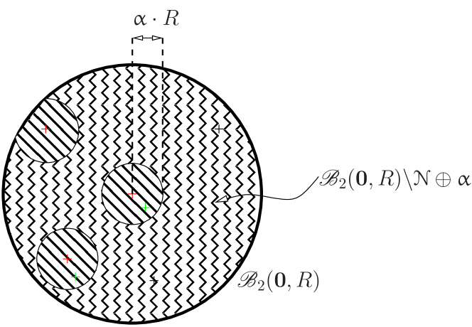
Figure 7: $q_{*}$ in eq. (114) measures the probability the a point drawn in ${\mathscr{B}}_{2}(\bm{0},R)$ escapes the neighborhoods of ${\mathcal{N}}\oplus\upalpha$. In this example, two points in black escape the neighborhoods (defined by three points in red), while two in green do not.

Assume that density ${\mathcal{D}}$ contains a $L_{2}$ ball ${\mathscr{B}_{2}}(\bm{0},R)$ of radius $R$, centered without loss of generality in $\bm{0}$. Fix $0<\upkappa<m-1$. For any $\upalpha\in(0,1)$ and ${\mathcal{N}}\subseteq{\mathcal{A}}$ with $|{\mathcal{N}}|\in\{1,2,...,\upkappa\}\stackrel{{\scriptstyle\mathrm{.}}}{{=}}[\upkappa]_{*}$, let ${\mathcal{N}}\oplus\upalpha\stackrel{{\scriptstyle\mathrm{.}}}{{=}}\cup_{\bm{x}\in{\mathcal{N}}}{\mathscr{B}_{2}}(\bm{x},\upalpha\cdot R)$ be the union of all small balls centered around each element of ${\mathcal{N}}$, each of radius $\upalpha\cdot R$. An important quantity is

$$q_{*} \stackrel{{\scriptstyle\mathrm{.}}}{{=}} \min_{{\mathcal{N}}\subseteq{\mathcal{A},|{\mathcal{N}}|\in[\upkappa]_{*}}}\frac{\mu({\mathscr{B}_{2}}(\bm{0},R)\backslash{\mathcal{N}}\oplus\upalpha)}{\mu({\mathscr{B}_{2}}(\bm{0},R))}$$ (114)

the minimal mass of ${\mathscr{B}_{2}}(\bm{0},R)\backslash{\mathcal{N}}\oplus\upalpha$ relatively to ${\mathscr{B}_{2}}(\bm{0},R)$ as measured using ${\mathcal{D}}$. As depicted in Figure 7, $q_{*}$ is a minimal value of the probability to escape the neighborhoods of ${\mathcal{N}}\oplus\upalpha$ when sampling points according to ${\mathcal{D}}$ in ball ${\mathscr{B}_{2}}(\bm{0},R)$. If, for some $\upalpha$ that shall depend upon the dimension $d$ and $\upkappa$, $q_{*}$ is large enough, then the spread of points drawn shall guarantee ”small” values for $\updelta_{w}$ and $\updelta_{s}$.

This is formalized in the following Theorem, which assumes $\upepsilon_{m}=\upepsilon_{M}=1$, i.e. the ball has uniform density. Theorem 10 is a direct consequence of this Theorem.

Theorem 25

Suppose ${\mathcal{A}}\subset{\mathscr{B}_{2}}(\bm{0},R)$. For any $\updelta\in(0,1)$, if

$$m \geq 3\left(\frac{\upkappa}{q_{*}\updelta^{2}}\right)^{2}\>\>,$$ (115)

then there is probability $\geq 1-\updelta$ over its sampling that ${\mathcal{A}}$ is $\updelta_{w}$-spread and $\updelta_{s}$-monotonic for the following values of $\updelta_{w},\updelta_{s}$:

$$\updelta_{w} = \frac{1}{q_{*}(1-\updelta)(m-\upkappa-1)\upalpha^{2}}\>\>,$$ (116)

$$\updelta_{s} = \frac{m}{m-\upkappa}\cdot\left(\frac{2}{\min\left\{\frac{1}{4},q_{*}(1-\updelta)\right\}\cdot\upalpha}\right)^{2}-1\>\>.$$ (117)

Proof.

We first prove the following Lemma.

Lemma 26

Suppose ${\mathcal{A}}\subset{\mathscr{B}_{2}}(\bm{0},R)$. Let $q_{*}$ be defined as in eq. (114). Then for any $\updelta\in(0,1)$, if $m$ meets ineq. (115), then there is probability $\geq 1-\updelta$ that

$$\left|({\mathscr{B}_{2}}(\bm{0},R)\backslash{\mathcal{N}}\oplus\upalpha)\cap({\mathcal{A}}\backslash{\mathcal{N}})\right| \geq q_{*}(1-\updelta)(m-\upkappa)\>\>,\forall{\mathcal{N}}\subseteq{\mathcal{A}},|{\mathcal{N}}|\in[\upkappa]_{*}\>\>.$$ (118)

Proof.

Since we assume ${\mathcal{A}}\subset{\mathscr{B}_{2}}(\bm{0},R)$, Chernoff bounds imply that for any fixed ${\mathcal{N}}\subseteq{\mathcal{A}}$ with $|{\mathcal{N}}|\in[\upkappa]_{*}$,

$$\mathbb{P}_{\mathcal{D}}\left[\frac{\left|({\mathscr{B}_{2}}(\bm{0},R)\backslash{\mathcal{N}}\oplus\upalpha)\cap({\mathcal{A}}\backslash{\mathcal{N}})\right|}{\left|{\mathcal{A}}\backslash{\mathcal{N}}\right|}\leq q_{*}(1-\updelta)\right] \leq \exp\left(-\updelta^{2}q_{*}\left|{\mathcal{A}}\backslash{\mathcal{N}}\right|/2\right)\>\>.$$ (119)

Now, remark that

$$\sum_{j=1}^{\upkappa}{m\choose j} \leq m^{\upkappa}\>\>,\forall m,\upkappa\geq 1\>\>.$$ (120)

This can be proven by induction, $m$ being fixed: it trivially holds for $\upkappa=1$ and $\upkappa=2$, and furthermore

$$\sum_{j=1}^{\upkappa}{m\choose j} = \sum_{j=1}^{\upkappa-1}{m\choose j}+{m\choose\upkappa}$$ (121)

$$\leq m^{\upkappa-1}+\frac{m!}{(m-\upkappa)!\upkappa!}\>\>,$$

by induction at rank $\upkappa-1$. To prove that the right-hand side of (121) is no more than $m^{\upkappa}$, we just have to remark that

$$\frac{m!}{(m-\upkappa)!\upkappa!m^{\upkappa-1}} < \frac{m}{\upkappa!}$$ (122)

$$\leq m-1\>\>,$$

as long as $\upkappa>1$ and $m>1$. So, the property at rank $\upkappa-1$ for $\upkappa>1$ implies property at rank $\upkappa$, which concludes the induction.

So, we have at most $m^{\upkappa}$ choices for ${\mathcal{N}}$, so relaxing the choice of ${\mathcal{N}}$, we get

$$\mathbb{P}_{\mathcal{D}}\left[\exists{\mathcal{N}}\subseteq{\mathcal{A}},|{\mathcal{N}}|=\upkappa:\frac{\left|({\mathscr{B}_{2}}(\bm{0},R)\backslash{\mathcal{N}}\oplus\upalpha)\cap{\mathcal{A}}_{\mathcal{N}}\right|}{\left|{\mathcal{A}}_{\mathcal{N}}\right|}\leq q_{*}(1-\updelta)\right]$$ (123)

$$\leq m^{\upkappa}\exp\left(-\frac{\updelta^{2}q_{*}(m-\upkappa)}{2}\right)\>\>.$$

We want to compute the minimal $m$ such that the right-hand side is no more than $\updelta$, this being equivalent to

$$\updelta^{2}q_{*}m \geq 2\log\left(\frac{m^{\upkappa}}{\updelta}\right)+\upkappa\updelta^{2}q_{*}\>\>,$$

which, since $\updelta\in(0,1)$, is ensured if

$$\updelta^{2}q_{*}m \geq 2\upkappa\log\left(\frac{m}{\updelta}\right)+\upkappa\updelta^{2}q_{*}\>\>.$$ (124)

Suppose

$$m = 3\left(\frac{\upkappa}{q_{*}\updelta^{2}}\right)^{2}\>\>.$$

Since we trivially have $\upkappa^{2}/(q_{*}\updelta^{2})^{2}\geq\upkappa\updelta^{2}q_{*}$ ($\upkappa\geq 1,q_{*}\in(0,1),\updelta\in(0,1)$), it is sufficient to prove:

$$\frac{2\upkappa}{q_{*}\updelta^{2}} \geq 2\log 3+2\log\left(\frac{\upkappa^{2}}{q^{2}_{*}\updelta^{5}}\right)\>\>,$$ (125)

which, again observing that $\updelta\in(0,1)$, holds if we can prove

$$\frac{\upkappa}{q_{*}\updelta^{2}} \geq \log 2+\frac{3}{2}\cdot\log\left(\frac{\upkappa}{q_{*}\updelta^{2}}\right)\>\>,$$ (126)

which is equivalent to showing $x\geq(3/2)\log x+\log 2$ for $x\geq 1$, which indeed holds (end of the proof of Lemma 26). ∎

The consequence of Lemma 26 is the following: if ${\mathcal{A}}\subset{\mathscr{B}_{2}}(\bm{0},R)$ and $m$ satisfies (115), then for any ${\mathcal{N}}\subseteq{\mathcal{A}}$ with $|{\mathcal{N}}|=k-1$, and any ${\mathcal{B}}\subseteq{\mathcal{A}}$ with $|{\mathcal{B}}|=|{\mathcal{A}}|-1$,

$$\sum_{\bm{a}\in{\mathcal{B}}}\|\bm{a}-\textsc{nn}_{\mathcal{N}}(\bm{a})\|_{2}^{2} \geq q_{*}(1-\updelta)(m-\upkappa-1)\upalpha^{2}\cdot R^{2}\>\>,$$ (127)

and so from Definition 7 ${\mathcal{A}}$ is $\updelta_{s}$-spread for:

$$\updelta_{w} = \frac{1}{q_{*}(1-\updelta)(m-\upkappa-1)\upalpha^{2}}\>\>.$$ (128)

Now, suppose we add a single point $\bm{x}_{*}$ in $\mathcal{N}$. If, for some fixed $\upalpha_{*}\in(0,\upalpha/2]$,

$$\bm{x}_{*} \not\in \bm{a}\oplus\upalpha_{*}\>\>,\forall\bm{a}\in{\mathcal{A}}\>\>,$$ (129)

then because of (127),

$$\sum_{\bm{a}\in{\mathcal{A}}}\|\bm{a}-\textsc{nn}_{{\mathcal{N}}\cup\{\bm{x}_{*}\}}(\bm{a})\|_{2}^{2} \geq (m-\upkappa)\cdot\min\left\{\upalpha_{*}^{2},q_{*}(1-\updelta)\upalpha^{2}\right\}\cdot R^{2}\>\>.$$ (130)

Otherwise, consider one $\bm{a}_{*}$ for which $\bm{x}_{*}\in\bm{a}_{*}\oplus\upalpha_{*}$. If we replace $\bm{a}_{*}$ by $\bm{x}_{*}$ in all ${\mathcal{N}}$ in which $\bm{a}_{*}$ belongs to in Lemma 26, then because $\bm{x}_{*}\oplus\upalpha_{*}\subset\bm{a}_{*}\oplus\upalpha$, it comes from Lemma 26:

$$\sum_{\bm{a}\in{\mathcal{A}}}\|\bm{a}-\textsc{nn}_{{\mathcal{N}}\cup\{\bm{x}_{*}\}}(\bm{a})\|_{2}^{2} \geq \frac{1}{4}\cdot(m-\upkappa)\cdot q_{*}(1-\updelta)\upalpha^{2}\cdot R^{2}\>\>.$$ (131)

We thus get in all cases

$$\sum_{\bm{a}\in{\mathcal{A}}}\|\bm{a}-\textsc{nn}_{\mathcal{N}\cup\{\bm{c}(A)\}}(\bm{a})\|_{2}^{2} \geq \min\left\{\frac{\upalpha^{2}}{4},\upalpha_{*}^{2},q_{*}(1-\updelta)\upalpha^{2}\right\}(m-\upkappa)\cdot q_{*}(1-\updelta)\cdot R^{2}\>\>,$$ (132)

where $\bm{c}(A)$ is the arithmetic average computed according to the definition of $\updelta_{s}$-monotonicity, of any $A\subseteq{\mathcal{A}}\backslash{\mathcal{N}}$. Since ${\mathcal{N}}\subseteq{\mathcal{A}}\subset{\mathscr{B}_{2}}(\bm{0},R)$, we have $\sum_{\bm{a}\in{\mathcal{A}}}\|\bm{a}-\textsc{nn}_{{\mathcal{N}}}(\bm{a})\|_{2}^{2}\leq 4mR^{2}$, and so

$$\sum_{\bm{a}\in{\mathcal{A}}}\|\bm{a}-\textsc{nn}_{{\mathcal{N}}}(\bm{a})\|_{2}^{2} \leq \frac{4m}{\min\left\{\frac{\upalpha^{2}}{4},\upalpha_{*}^{2},q_{*}(1-\updelta)\upalpha^{2}\right\}(m-\upkappa)\cdot q_{*}(1-\updelta)}\cdot\sum_{\bm{a}\in{\mathcal{A}}}\|\bm{a}-\textsc{nn}_{\mathcal{N}\cup\{\bm{c}(A)\}}(\bm{a})\|_{2}^{2}\>\>,$$ (133)

implying from Definition 8 that $\updelta_{s}$-monotonicity holds with:

$$\updelta_{s} = \frac{m}{m-\upkappa}\cdot\frac{4}{\min\left\{\frac{\upalpha^{2}}{4},\upalpha_{*}^{2},q_{*}(1-\updelta)\upalpha^{2}\right\}\cdot q_{*}(1-\updelta)}-1\>\>.$$ (134)

The statement of the Theorem follows with $\upalpha_{*}=\upalpha/2$ (end of the proof of Theorem 25). ∎

We finish the proof of Theorem 10. We have

$$q_{*} \geq 1-\upkappa\upalpha^{d}\>\>,$$ (135)

where the lowerbound corresponds to the case where all neighborhoods in ${\mathcal{N}}\oplus\upalpha$ are distinct and included in ${\mathscr{B}_{2}}(\bm{0},R)$. So we have, for any fixed choice of $\upalpha\in(0,1)$,

$$\updelta_{w} \leq \frac{1}{\upalpha^{2}\cdot(1-\upkappa\upalpha^{d})(1-\updelta)(m-\upkappa-1)}\>\>.$$ (136)

To minimize this upperbound, we pick $\upalpha$ to maximize $\upalpha^{2}\cdot(1-\upkappa\upalpha^{d})$ with $\upalpha\in(0,1)$, which is easily achieved picking

$$\upalpha = \left(\frac{1}{\upkappa(d+1)}\right)^{\frac{1}{d}}\>\>,$$ (137)

and yields

$$\updelta_{w} \leq \left(1+\frac{1}{d}\right)\cdot\frac{1}{(\upkappa(d+1))^{\frac{2}{d}}(1-\updelta)(m-\upkappa-1)}$$ (138)

$$\leq \left(1+\frac{1}{d}\right)\cdot\frac{1}{\upkappa^{\frac{2}{d}}(1-\updelta)(m-\upkappa-1)}\>\>.$$

But we have for this choice, $1-\upkappa\upalpha^{d}=d/(d+1)\geq 1/2$, so as long as

$$\updelta<1/2\>\>,$$ (139)

we shall have $q_{*}(1-\updelta)>1/4$ and so we shall have

$$\updelta_{s}+1 = 64\cdot\frac{m}{m-\upkappa}\cdot\frac{1}{\upalpha^{2}}$$ (140)

$$\leq 64\cdot\frac{m}{m-\upkappa}\cdot\frac{1}{\upkappa^{\frac{2}{d}}}\>\>.$$

We now go back to ineq. (16), which reads:

$$\frac{\mathbb{P}[{\mathcal{C}}|{\mathcal{A}}^{\prime}]}{\mathbb{P}[{\mathcal{C}}|{\mathcal{A}}]}\leq\varrho_{1}+\varrho_{2}\>\>,$$ (141)

with

$$\varrho_{1} \stackrel{{\scriptstyle\mathrm{.}}}{{=}} (1+\updelta_{w})^{k-1}\>\>,$$ (142)

$$\varrho_{2} \stackrel{{\scriptstyle\mathrm{.}}}{{=}} f(k)\cdot\updelta_{w}\cdot\left(1+\updelta_{s}\right)^{k-1}\cdot\varrho(R)\>\>.$$ (143)

We upperbound separately both terms.

Lemma 27

Suppose ineqs (139) and (17) are met. Then

$$\varrho_{1} \leq 1+\frac{4}{m^{\frac{1}{4}+\frac{1}{d+1}}}\>\>.$$ (144)

Proof.

Since $d\geq 1$ and $\updelta<1/2$, we get from ineq. (138) (using $\upkappa=k$)

$$(1+\updelta_{w})^{k-1} \leq \left(1+\left(1+\frac{1}{d}\right)\cdot\frac{1}{k^{\frac{2}{d}}(1-\updelta)(m-k-1)}\right)^{k-1}$$ (145)

$$\leq \left(1+\frac{2}{k^{\frac{2}{d}}(1-\updelta)(m-k-1)}\right)^{k-1}$$

$$\leq \left(1+\frac{4}{k^{\frac{2}{d}}(m-k-1)}\right)^{k-1}\>\>.$$

Let $h(k)$ be the right-hand side of ineq. (145). $h(1)$ trivially meets ineq. (144). When $k\geq 2$, $h$ decreases until $k=2(m-1)/(d+2)$ and then increases. We thus just need to check ineq. (144) for $k=2$ and $k=\sqrt{m}$ from ineq. (17). We get $h(2)=1+4/(4^{1/d}(m-3))$. For ineq. (144) to be satisfied, we need to have $4^{1/d}(m-3)\geq m^{\frac{1}{4}+\frac{1}{d+1}}$, which holds if $m\geq 3+m^{3/4}$ ($d\geq 1$), that is, $m\geq 8$. But since ineqs (139) and (17) are satisfied, we have $m\geq 16k^{2}/\updelta^{2}\geq 64k^{2}\geq 64$, and so $h(2)$ satisfies ineq. (144).

There remains to check ineq. (144) for $k=\sqrt{m}$. We have

$$h(\sqrt{m}) = \left(1+\frac{4}{m^{\frac{1}{d}}(m-\sqrt{m}-1)}\right)^{\sqrt{m}-1}$$ (146)

$$\leq \left(1+\frac{4}{m^{\frac{1}{d}}(m-\sqrt{m})}\right)^{\sqrt{m}}$$

$$\leq \left(1+\frac{2}{\sqrt{m}\cdot m^{\frac{1}{4}+\frac{1}{d}}}\right)^{\sqrt{m}}\>\>,$$

since any $m\geq 64$, we have $m-\sqrt{m}\geq 2m^{3/4}$. To conclude, ineq (146) yields

$$h(\sqrt{m}) \leq \left(1+\frac{2}{\sqrt{m}\cdot m^{\frac{1}{4}+\frac{1}{d}}}\right)^{\sqrt{m}}$$ (147)

$$\leq \exp\left(\frac{2}{m^{\frac{1}{4}+\frac{1}{d}}}\right)$$

$$\leq 1+\frac{4}{m^{\frac{1}{4}+\frac{1}{d}}}\>\>.$$

The penultimate ineq. comes from $1+x\leq\exp x$, and the last one comes from the fact that $\exp(2x)\leq 1+4x$ for $x\leq 1$. Since $m^{\frac{1}{4}+\frac{1}{d}}\geq m^{\frac{1}{4}+\frac{1}{d+1}}$, we obtain the statement of the Lemma for $h(\sqrt{m})$. This concludes the proof of Lemma 27. ∎

Lemma 28

Suppose ineqs (139) and (17) are met. Then

$$\varrho_{2} \leq \left(\frac{64}{k^{\frac{2}{d}}}\right)^{k}\cdot\frac{\varrho(2R)}{m}\>\>.$$ (148)

Proof.

We fix $\upkappa=k$, use $f(k)=4^{2k-4}$ (eq. 113), so we get

$$\varrho_{2} = 4^{2k-2}\cdot\left(1+\frac{1}{d}\right)\cdot\frac{1}{k^{\frac{2}{d}}(1-\updelta)(m-k-1)}\cdot\left(64\cdot\frac{m}{m-k}\cdot\frac{1}{k^{\frac{2}{d}}}\right)^{k-1}\cdot\varrho(2R)$$ (149)

$$\leq 2\cdot 64^{k-1}\cdot\left(1+\frac{1}{d}\right)\cdot\frac{1}{k^{\frac{2k}{d}}(m-k-1)}\cdot\left(1+\frac{k}{m-k}\right)^{k-1}\cdot\varrho(2R)$$

$$\leq \underbrace{4\cdot\frac{1}{(m-k-1)}\cdot\left(1+\frac{k}{m-k}\right)^{k-1}}_{\stackrel{{\scriptstyle\mathrm{.}}}{{=}}\varrho_{3}}\cdot 64^{k-1}\cdot\frac{1}{k^{\frac{2k}{d}}}\cdot\varrho(2R)\>\>,$$ (150)

using the fact that $\updelta<1/2$ and $d\geq 1$. Now, we also have

$$\left(1+\frac{k}{m-k}\right)^{k-1} \leq \exp\left(\frac{k^{2}}{m-k}\right)\noindent$$ (151)

$$\leq e\>\>,$$ (152)

as long as $k\leq(1/16)\cdot\sqrt{m}$, and furthermore, since $m\geq 64$ (see the proof of Lemma 27), we also have $1/(m-k-1)\leq 5/m$. We thus obtain

$$\varrho_{3} \leq \frac{20e}{m}$$ (153)

$$\leq \frac{64}{m}\>\>,$$

which yields

$$\varrho_{2} \leq \left(\frac{64}{k^{\frac{2}{d}}}\right)^{k}\cdot\frac{\varrho(2R)}{m}\>\>,$$ (154)

as claimed. ∎

Putting altogether Lemmata 27 and 28, we get:

$$\frac{\mathbb{P}[{\mathcal{C}}|{\mathcal{A}}^{\prime}]}{\mathbb{P}[{\mathcal{C}}|{\mathcal{A}}]} \leq 1+\frac{4}{m^{\frac{1}{4}+\frac{1}{d+1}}}+\left(\frac{64}{k^{\frac{2}{d}}}\right)^{k}\cdot\frac{\varrho(2R)}{m}\>\>,$$ (155)

as claimed. There remains to check that, with our choice of $\upalpha$, the constraint on $m$ in (115) is satisfied if

$$m \geq \frac{12k^{2}}{\updelta^{4}}$$ (156)

since $q_{*}\geq d/(d+1)$. We obtain the sufficient constraint on $k$:

$$k \leq \frac{\updelta^{2}}{4}\cdot\sqrt{m}\>\>,$$ (157)

which proves Theorem 10 when $\upepsilon_{m}=\upepsilon_{M}=1$.

When the density do not satisfy $\upepsilon_{m}=\upepsilon_{M}=1$ we just have to remark that the lowerbound on $q_{*}$ is now

$$q_{*} \leq \frac{\varepsilon_{m}}{\varepsilon_{M}}\cdot(1-\upkappa\upalpha^{d})\>\>.$$ (158)

Ineq. (138) becomes

$$\updelta_{w} \leq \frac{\varepsilon_{M}}{\varepsilon_{m}}\cdot\left(1+\frac{1}{d}\right)\cdot\frac{1}{\upkappa^{\frac{2}{d}}(1-\updelta)(m-\upkappa-1)}\>\>,$$ (159)

ineq. (140) becomes

$$\updelta_{s}+1 \leq \frac{\varepsilon_{M}}{\varepsilon_{m}}\cdot 64\cdot\frac{m}{m-\upkappa}\cdot\frac{1}{\upkappa^{\frac{2}{d}}}\>\>.$$ (160)

So, the only difference with the $\upepsilon_{m}=\upepsilon_{M}=1$ is the ratio $\varepsilon_{M}/\varepsilon_{m}$ ($\geq 1$) which multiplies all quantities of interest, and yields, in lieu of ineq. (155),

$$\frac{\mathbb{P}[{\mathcal{C}}|{\mathcal{A}}^{\prime}]}{\mathbb{P}[{\mathcal{C}}|{\mathcal{A}}]} \leq 1+\left(\frac{\varepsilon_{M}}{\varepsilon_{m}}\right)^{k}\cdot\left(\frac{4}{m^{\frac{1}{4}+\frac{1}{d+1}}}+\left(\frac{64}{k^{\frac{2}{d}}}\right)^{k}\cdot\frac{\varrho(2R)}{m}\right)\>\>,$$ (161)

which is the statement of Theorem 10.

Proof of Theorem 12

When $p_{(\bm{\mu}_{\bm{a}},\bm{\theta}_{\bm{a}})}$ is a product of Laplace distributions $Lap(b)$ ($b$ being the scale parameter of the distribution (Dwork & Roth, 2014)), condition in ineq. (15) becomes:

$$\frac{p_{(\bm{\mu}_{\bm{a}^{\prime}},\bm{\theta}_{\bm{a}^{\prime}})}(\bm{x})}{p_{(\bm{\mu}_{\bm{a}},\bm{\theta}_{\bm{a}})}(\bm{x})} \leq \exp\left(\frac{\|\bm{a}-\bm{a}^{\prime}\|_{1}}{b}\right)$$ (162)

$$=\exp\left(\frac{\sqrt{2}\|\bm{a}-\bm{a}^{\prime}\|_{1}}{\sigma_{1}}\right)$$

$$\leq \exp\left(\frac{2\sqrt{2}R}{\sigma_{1}}\right)\>\>,\forall{\bm{a}},{\bm{a}^{\prime}}\in{\mathcal{A}},\forall\bm{x}\in\Omega\>\>,$$

assuming ${\mathcal{A}}\subset{\mathscr{B}}_{1}(\bm{0},R)$. Let us fix $\varrho(R)\stackrel{{\scriptstyle\mathrm{.}}}{{=}}\exp\left(2\sqrt{2}R/\sigma_{1}\right)$. Since ${\mathscr{B}}_{1}(\bm{0},R)\subset{\mathscr{B}}_{2}(\bm{0},R)$ (the $L_{2}$ ball), we now want $(1+\updelta_{w})^{k-1}+f(k)\cdot\updelta_{w}\cdot\left(1+\updelta_{s}\right)^{k-1}\cdot\varrho(R)=\exp(\epsilon)$. Solving for $\sigma_{1}$ yields:

$$\sigma_{1} = \frac{2\sqrt{2}R}{\log\left(\frac{\exp(\epsilon)-(1+\updelta_{w})^{k-1}}{f(k)\cdot\updelta_{w}\cdot\left(1+\updelta_{s}\right)^{k-1}}\right)}\>\>,$$ (163)

as claimed. The proof that $k$-variates++ meets ineq. (7) with

$$\Phi = \Phi_{1}\stackrel{{\scriptstyle\mathrm{.}}}{{=}}8\cdot\left(\phi_{{\tiny\mathrm{opt}}}+\frac{mR^{2}}{\tilde{\epsilon}^{2}}\right)$$ (164)

comes from a direct application of Theorem 2, with

$$\upeta = 0\>\>,$$

$$\phi_{{\tiny\mathrm{bias}}} = \phi_{{\tiny\mathrm{opt}}}\>\>,$$

$$\phi_{{\tiny\mathrm{var}}} = m\cdot\left(\frac{2\sqrt{2}R}{\tilde{\epsilon}}\right)^{2}\>\>.$$

The statements for $\sigma_{2}$ and $\Phi_{2}$ are direct applications of the Laplace mechanism properties (Dwork & Roth, 2014; Dwork et al., 2006).

Extension to non-metric spaces

Since its inception, the $k$-means++ seeding technique has been successfully adapted to various distortion measures $D(\cdot\|\cdot)$ to handle non-Euclidean features (Jegelka et al., 2009; Nock et al., 2008, 2016). Similarly, our extended seeding technique can be adapted to these scenarii: this boils down to putting the distortion as a free parameter of the algorithm, replacing $D_{t}(\bm{a})$ (eq. (1)) by $D_{t}(\bm{a})\stackrel{{\scriptstyle\mathrm{.}}}{{=}}\min_{\bm{a}^{\prime}\in{\mathcal{P}}}D(\bm{a}\|\bm{a}^{\prime})$. For example, by noticing that the squared Euclidean distance is merely an example of Bregman divergences (the well-known canonical divergences in information geometry of dually flat spaces), $k$-variates++ can be been extended to that family of dissimilarities (Nock et al., 2008). But more interesting examples now appear, that build on constraints that distortions have to satisfy for certain problems, like the invariance to rotations of the coordinate space. This is all the more challenging in practice for clustering since sometimes no-closed form solution are available for some of these divergences. Because it bypasses the construction of the population minimisers, $k$-variates++ offers an elegant solution to the problem. Such hard distortions include the skew Jeffreys $\alpha$-centroids (Nock et al., 2016). This also include the recent class of total Bregman/Jensen divergences that are examples of conformal divergences (Nielsen & Nock, 2015; Nock et al., 2016). We give an example of the extension of $k$-variates++to the total Jensen divergence, to show that $k$-variates++ can approximate the optimal clustering even without closed form solutions for the population minimisers (Nielsen & Nock, 2015). For any convex function $\varphi:{\mathbb{R}}^{d}\rightarrow{\mathbb{R}}$ and $\alpha\in(0,1)$, the skew Jensen divergence is

$$J_{\alpha}(\bm{a},\bm{a}^{\prime}) \stackrel{{\scriptstyle\mathrm{.}}}{{=}} \alpha\varphi(\bm{a})+(1-\alpha)\varphi(\bm{a}^{\prime})-\varphi(\alpha\bm{a}+(1-\alpha)\bm{a}^{\prime})\>\>,$$ (165)

and the total Jensen divergence is

$$tJ_{\alpha}(\bm{a},\bm{a}^{\prime}) \stackrel{{\scriptstyle\mathrm{.}}}{{=}} \frac{1}{\sqrt{1+U^{2}}}\cdot J_{\alpha}(\bm{a},\bm{a}^{\prime})\>\>,$$ (166)

where $U\stackrel{{\scriptstyle\mathrm{.}}}{{=}}(\varphi(\bm{a})-\varphi(\bm{a}^{\prime}))/\|\bm{a}-\bm{a}^{\prime}\|_{2}$. There is no closed form solution for the population minimiser of $tJ_{\alpha}$, yet we can prove the following Theorem, which builds upon Theorem 3 in (Nielsen & Nock, 2015).

Theorem 29

In $k$-variates++, replace $D_{t}(\bm{a})$ (eq. (1)) by $D_{t}(\bm{a})\stackrel{{\scriptstyle\mathrm{.}}}{{=}}\min_{\bm{a}^{\prime}\in{\mathcal{P}}}tJ_{\alpha}(\bm{a},\bm{a}^{\prime})$ ans suppose for simplicity that probe functions are identity: $\wp_{t}=\mathrm{Id},\forall t$. Denote $\phi_{{\tiny\mathrm{opt}}}$ the optimal noise-free potential of the clustering problem using $tJ_{\alpha}$ as distortion measure. Then there exists a constant $\upomega>0$ such that for any choice of densities $p_{\bm{\mu}_{.},\bm{\theta}_{.}}$, the expected $tJ_{\alpha}$-potential $\phi$ of $k$-variates++ satisfies:

$$\mathbb{E}[\phi({\mathcal{A}};{\mathcal{C}})] \leq \upomega\cdot\log k\cdot\left(6\phi_{{\tiny\mathrm{opt}}}+2\phi_{{\tiny\mathrm{bias}}}+2\phi_{{\tiny\mathrm{var}}}\right)\>\>,$$ (167)

where $\phi_{{\tiny\mathrm{var}}}$ is defined in Theorem 2 and $\phi_{{\tiny\mathrm{bias}}}$ is defined in eq. (4).

9 Appendix on Experiments

Experiments on Theorem 12 and the sublinear noise regime

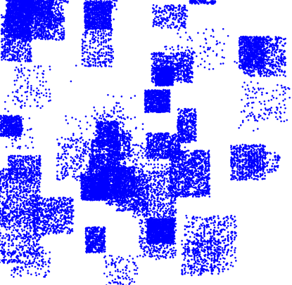
Figure 8: Final dataset for the experiments in Table 4 (plot of the two first coordinates ($d=10$)).

$\epsilon=0.1$	$\epsilon=1$	$\epsilon=10$

Table 4: Case $d=10,k=3$ — Plot of $\tilde{\epsilon}$ as in Theorem 12 (see also eq. (168) below) and best fit for model $\tilde{\epsilon}=a+b\log m$. Figure 8 displays the final dataset obtained (see text).

$\epsilon=0.1$	$\epsilon=1$	$\epsilon=10$

Table 5: Case $d=50,k=3$ — Plot of $\tilde{\epsilon}$ as in Theorem 12 (see also eq. (168) below) and best fit for model $\tilde{\epsilon}=a+b\log m$. All other parameters are the same as for Table 4.

$\epsilon=0.1$	$\epsilon=1$	$\epsilon=10$

Table 6: Case $d=50,k=4$ — Plot of $\tilde{\epsilon}$ as in Theorem 12 (see also eq. (168) below) and best fit for model $\tilde{\epsilon}=a+b\log m$. All other parameters are the same as for Table 4.

$\hookrightarrow$ comments on $\tilde{\epsilon}$

An important parameter of Theorem 12 is $\tilde{\epsilon}$, which replaces $\epsilon$ in the computation of the noise standard deviation in $\sigma_{1}$: the larger it is compared to $\epsilon$, the less noise we can put while still ensuring $\mathbb{P}[{\mathcal{C}}|{\mathcal{A}}^{\prime}]/\mathbb{P}[{\mathcal{C}}|{\mathcal{A}}]\leq\exp\epsilon$ in Definition 11. Recall its formula:

$$\tilde{\epsilon} \stackrel{{\scriptstyle\mathrm{.}}}{{=}} \log\left(\frac{\exp(\epsilon)-(1+\updelta_{w})^{k-1}}{f(k)\cdot\updelta_{w}\cdot\left(1+\updelta_{s}\right)^{k-1}}\right)\>\>.$$ (168)

The experimental setting is the following one: we repeatedly sample clusters that are uniform in a subset of the domain (with limited, random size), taken to be a $d$-dimensional hyperrectangle of randomly chosen edge lengths. Each cluster contains a randomly picked number of points between 1 and 1000. After each cluster is picked, we updated an estimation of $\updelta_{w}$ and $\updelta_{s}$:

• we compute $\updelta_{w}$ by randomly picking ${\mathcal{B}}$ and ${\mathcal{N}}$ for a total number of $n_{{\tiny\mathrm{est}}}$ iterations, with $n_{{\tiny\mathrm{est}}}=5000$;

• we compute $\updelta_{s}$ by randomly picking ${\mathcal{N}}$ for a total number of $n_{{\tiny\mathrm{est}}}$ iterations. Instead of computing $A$ then $\bm{x}$, we opt for the fast proxy which consists in replacing $\bm{c}(A)$ by a random data point, thus without making the ${\mathcal{N}}$-packed test. This should reasonably overestimate $\updelta_{s}$ and thus slightly loosen our approximation bounds.

Figure 8 shows the dataset obtained for $d=10$ at the end of the process. Predictably, the distribution on the whole space looks like a highly non-uniform cover by locally uniform clusters. Tables 4, 5 and 6 display results obtained for three different values of $\epsilon$ and three different values for the couple $(d,k)$. To test the large sample regime intuition and the fact that the the noise dependence grows sublinearly in $m$, we have regressed in each plot $\tilde{\epsilon}$ as a function of $m$ for

$$\tilde{\epsilon}(m) = a+b\log m\>\>.$$ (169)

The plots obtained confirm a good approximation of this intuition, but they also display some more good news. The smaller $\epsilon$, the larger can be $\tilde{\epsilon}$ relatively to $\epsilon$, by order of magnitudes if $\epsilon$ is small. Hence, despite the fact that we evetually overestimate $\updelta_{s}$, we still get large $\tilde{\epsilon}$. Furthermore, if $k$ is small, this ”large sample” regime in which $\tilde{\epsilon}>\epsilon$ actually happens for quite small values of $m$.

Also, one may remark that the curves all look like an approximate translation of the same curve. This is not surprising, since we can reformulate

$$\tilde{\epsilon} = \epsilon+\log\left(1-\frac{U}{\epsilon}\right)+g(m)\>\>,$$ (170)

whene $U\stackrel{{\scriptstyle\mathrm{.}}}{{=}}(1+\updelta_{w})^{k-1}$ and $g$ do not depend on $\epsilon$. It happens that $\updelta_{w}$ quickly decreases to very small values (bringing also a separate empirical validation of its behavior as computed in ineq. (159) in the proof of Theorem 10). Hence, we rapidly get for small $m$ some $\tilde{\epsilon}$ that looks like

$$\tilde{\epsilon} \approx \epsilon+\log\left(1-\frac{1+o(1)}{\epsilon}\right)+g(m)$$ (171)

$$\approx h(\epsilon)+g(m)\>\>,$$

which may explain what is observed experimentally.

We can sumarise the global picture for $\tilde{\epsilon}$ vs $\epsilon$ by saying that it becomes more and more in favor of $\tilde{\epsilon}$ as data size ($d$ or $m$) increase, but become less in favor of $\tilde{\epsilon}$ as the number of clusters $k$ increases (predictably).

	$(d,k)=(10,3)$	$(d,k)=(50,3)$	$(d,k)=(50,4)$
$\updelta_{w}$
$\updelta_{s}$

Table 7: Estimations of $\updelta_{w}$ (top row) and $\updelta_{s}$ (bottom row) as a function of $m$, for three values of $(d,k)$. We also indicate the best fit for $\updelta_{w}(m)=a/m$ (top row) and $\updelta_{s}(m)=b$ (for $m\geq 4000$, bottom row).

$\hookrightarrow$ comments on $\updelta_{w}$ and $\updelta_{s}$

Table 7 presents the estimated values of $\updelta_{w}$ and $\updelta_{s}$ for the settings of Tables 4, 5 and 6. We wanted to test the intuition as to whether, for $m$ sufficiently large, it would hold that $\updelta_{w}=O(1/m)$ while $\updelta_{s}=O(1)$. The essential part is on $\updelta_{w}$, since such a behaviour would be sufficient for the sublinear growth of the noise dependence. One can check that such behaviours are indeed observed, and more: $\updelta_{w}$ converges very rapidly to zero, at least for all settings in which we have tested data generation. Another quite good news, is that $\updelta_{s}$ seems indeed to be $\theta(1)$, but for an actual value which is also not large, so the denominator of eq. (168) is actually driven by $f(k)$, even when, as we already said, we may have a tendency to overestimate $\updelta_{s}$ with our randomized procedure.

Experiments with d$k$-means++, $k$-means++ and $k$-means${}_{\tiny{\mbox{$\|$}}}$

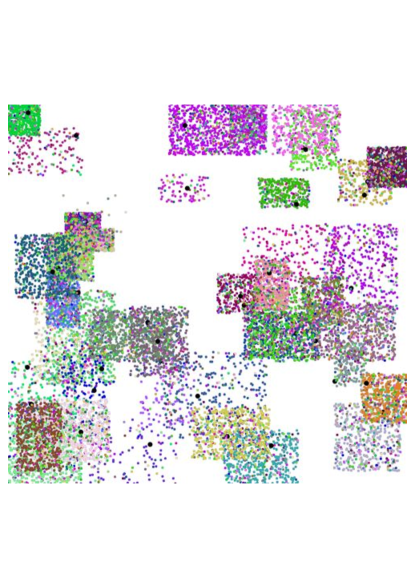
Figure 9: Example dataset obtained for $p=50\%$ ($d=50$). Each color represents the points held by a peer (Forgy node) after the process of moving each point from a true cluster to another cluster with probability $p=0.5$. Big black dots are the datapoints that are the closet to the true cluster centers.

$k=4$	$k=5$	$k=6$	$k=7$	$k=8$	$k=9$	$k=10$

Table 8: Simulated data — Plot of ratio $\uprho_{\phi}(\mbox{$k$-means++})$ in eq. (172) as a function of $\phi_{s}^{F}$. Points below the green line correspond to (average) runs in which d$k$-means++ beats $k$-means++.

$k=4$	$k=5$	$k=6$	$k=7$	$k=8$	$k=9$	$k=10$

Table 9: Simulated data — Plot of ratio $\uprho_{\phi}(\mbox{$k$-means${}_{\tiny{\mbox{$\|$}}}$})$ in eq. (172) as a function of $\phi_{s}^{F}$. Points below the green line correspond to (average) runs in which d$k$-means++ beats $k$-means${}_{\tiny{\mbox{$\|$}}}$.

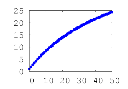
Figure 10: Simulated data — Relative increase of spread, $\phi_{s}^{F}(p)/\phi_{s}^{F}(0)$, through the runs, as a function of $p$.

$\star$ Experiments on synthetic data

We have generated a set of $m\approx$20 000 points using the same kind of clusters as in the experiments related to Theorem 12: we add ”true” clusters until the total number of points exceeds 20 000. To simulate the spread of data among peers (Forgy nodes) and evaluate the influence of the spread of Forgy nodes ($\phi_{s}^{F}$) for d$k$-means++, we have devised the following protocol: let us name ”true” clusters the hyperrectangle clusters used to build the dataset. Each true cluster corresponds to the data held by a peer. Then, for some $p\in[0,100]$ ($\%$), each point in each true cluster moves into another cluster, with probability $p$. The choice of the target cluster is made uniformly at random. Thus, as $p$ increases, we get a clustering problem in which the data held by peers is more and more spread, and for which the spread of Forgy nodes $\phi_{s}^{F}$ increases. Figure 9 presents a typical example of the spread for $p=50\%$. Notice that in this case many Forgy nodes have data spreading through a much larger domain than the initial, true clusters. Figure 10 displays that this happens indeed, as $\phi_{s}^{F}$ is multiplied by a factor exceeding 20 (compared to $\phi_{s}^{F}$ at $p=0$) for the largest values of $p$.

We have compared d$k$-means++ to $k$-means++ and $k$-means${}_{\tiny{\mbox{$\|$}}}$ (Bahmani et al., 2012). In the case of that latter algorithm, we follow the paper’s statements and pick the number of outer iterations to be $\lceil\log\phi_{1}\rceil$, where $\phi_{1}$ is the potential for one Forgy-chosen center. We also pick $\ell=2k$, considering that it is a value which gives some of the best experimental results in (Bahmani et al., 2012). Finally, we recluster the points at the end of the algorithm using $k$-means++. For each algorithm ${\mathcal{H}}\in\{$k$\mbox{-means++},\mbox{$k$-means${}_{\tiny{\mbox{$\|$}}}$}\}$, we run it on the complete dataset and its results are averaged over 10 runs. We run d$k$-means++ for each $p\in\{0\%,1\%,...,50\%\}$. More precisely, for each $p$, we average the results of d$k$-means++ over 10 runs. We use as metric the relative increase in the potential of d$k$-means++ compared to ${\mathcal{H}}$:

$$\uprho_{\phi}({\mathcal{H}}) \stackrel{{\scriptstyle\mathrm{.}}}{{=}} \frac{\phi(\mbox{{d}$k$-means++})-\phi({\mathcal{H}})}{\phi({\mathcal{H}})}\cdot 100\>\>.$$ (172)

that we plot as a function of $\phi_{s}^{F}$, or surface plot as a function of $(k,p)$. The intuition for the former plot is that the larger $\phi_{s}^{F}$, the larger should be this ratio, since the data held by peers spreads across the domain and each peer is constrained to pick its centers with uniform seeding.

$\hookrightarrow$ d$k$-means++ vs $k$-means++

Figure 8 presents results for $\uprho_{\phi}(\mbox{$k$-means++})=f(\phi_{s}^{F})$ obtained for various $k$. First, the intuition is indeed confirmed for $k=8,9,10$, but an interesting phenomenon appears for $k=5$: d$k$-means++ almost consistently beats $k$-means++. The decrease in the average potential ranges up to $3\%$. Furthermore, this happens even for large values of $\phi_{s}^{F}$. Finally, for all but one value of $k$, there exists spread values for which d$k$-means++ beats $k$-means++. The surface plot in Figure 3 displays that superior performances of d$k$-means++ are probably not random. One possible explanation to this phenomenon relies on the expression of $\phi_{{\tiny\mathrm{bias}}}$ given in the proof of Theorem 4 (eq. (54)), recalled here:

$$\phi_{{\tiny\mathrm{bias}}} \stackrel{{\scriptstyle\mathrm{.}}}{{=}} \sum_{\bm{a}\in{\mathcal{A}}}\|\bm{\mu}_{\bm{a}}-\bm{c}_{{\tiny\mathrm{opt}}}(\bm{a})\|_{2}^{2}$$

$$= \sum_{i\in[n]}\sum_{\bm{a}\in{\mathcal{A}}_{i}}\|\bm{c}({\mathcal{A}}_{i})-\bm{c}_{{\tiny\mathrm{opt}}}(\bm{a})\|_{2}^{2}\>\>.$$

Recall that $\phi_{{\tiny\mathrm{bias}}}$ can be $<\phi_{{\tiny\mathrm{opt}}}$, and it can even be zero, in which case Theorem 2 says that the approximation bound may actually be better than that of $k$-means++ in (Arthur & Vassilvitskii, 2007) (furthermore, $\upeta=0$ for d$k$-means++). Hence, what happens is pobably that in several cases, there exists a union of peers data (the number of peers is larger than $k$) that gives a at least reasonably good approximation of the global optimum. In all our experiments indeed, we obtained a number of peers larger than 30.

$\hookrightarrow$ d$k$-means++ vs $k$-means${}_{\tiny{\mbox{$\|$}}}$

Figure 3 appear to display performances for d$k$-means++ that are even more in favor of d$k$-means++, compared to $k$-variates++. Figure 9 presents results for $\uprho_{\phi}(\mbox{$k$-means${}_{\tiny{\mbox{$\|$}}}$})=f(\phi_{s}^{F})$ obtained for various $k$. The fact that each of them is a vertical translation of a picture in Figure 8 comes from the fact that the results of $k$-means${}_{\tiny{\mbox{$\|$}}}$ and $k$-means++ do not depend on the spread of the neighbors $\phi_{s}^{F}$.

$\star$ Experiments on real world data

We consider the EuropeDiff dataset (Dataset characteristics provided in Table 10). Figures 11 and 12 give the results for the equivalent settings of the experimental data. To simulate $N$ peers with real data, reasonably spread geographically, we have sampled $N$ points (”peer centers”) with $k$-means++ seeding in data and then aggregated for each peer the subset of data in the corresponding Voronoi 1-NN cell. We then simulate the spread for parameter $p$ as in the simulated data. Figures 11 and 12 globally display (and confirm) the same trends as for the simulated data. They, however, clearly emphasize this time that the spread of Forgy nodes $\phi_{s}^{F}$ is one key parameter that drives the performances of d$k$-means++. Notice also that d$k$-means++ remains on this dataset competitive up to $p\geq 30\%$, which means that it remains competitive when a significant proportion of peers’ data is scattered without any constraint.

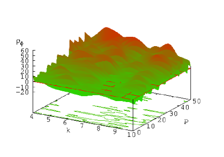
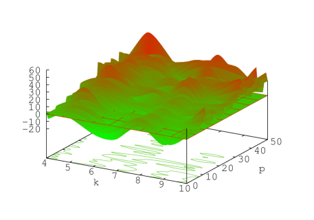
$\uprho_{\phi}(\mbox{$k$-means++})$	$\uprho_{\phi}(\mbox{$k$-means${}_{\tiny{\mbox{$\|$}}}$})$

$k=4$	$k=5$	$k=6$	$k=7$	$k=8$	$k=9$	$k=10$

$k=4$	$k=5$	$k=6$	$k=7$	$k=8$	$k=9$	$k=10$

Figure 11: Experiments on real world data ”EuropeDiff” with $N=30$ simulated peers. Top plot: Plots corresponding to Figure 3. Middle and bottom plot ranges: plots corresponding respectively to Figures 8 and 9.

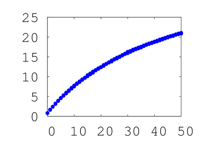
Figure 12: Experiments on real world data ”EuropeDiff” with $N=40$ simulated peers. Plot corresponding to Figure 10.

To further address the way the spread of Forgy nodes affects results, we have used another real world data with highly non-uniform distribution, Mopsi-Finland locations ($m=13467,d=2$). We have sampled peers using two different schemes for the peer centers: $k$-means++ and Forgy. In this latter initialisation, we just pick peer centers at random. In the former $k$-means++ initialisation, the initial peer centers are much more evenly geographically spread before we complete the peers data with the closest points. They remain more spread after the $p\%$ uniform displacement of data between peers, as shown on the top plots of Figure 13. What is interesting about this data is that it displays that if peers’ data are indeed geographically located, then d$k$-means++ is competitive up to quite reasonable values of $p\leq 20\%$ (depending on $k$). That, is d$k$-means++ works well when each peer aggregates 80 $\%$ data which is reasonably ”localized in the domain” and 20 $\%$ data which can be located everywhere in the domain.

Forgy initial peer centers	$k$-means++ initial peer centers

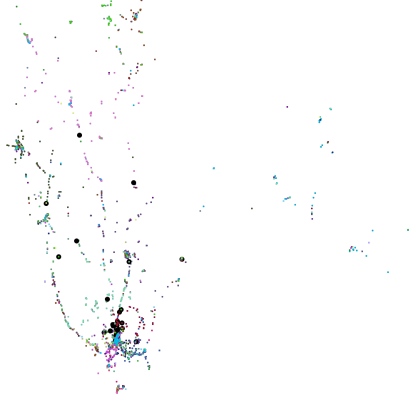
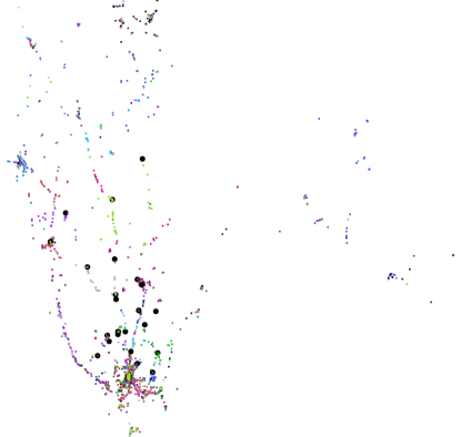
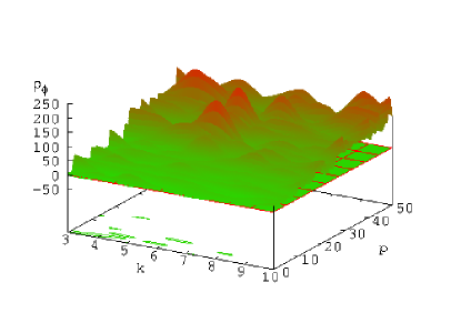
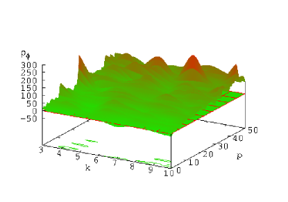
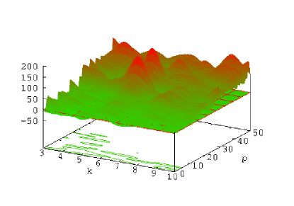
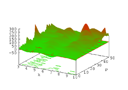
Figure 13: Mopsi-Finland locations data — Top: peer centers (big black dots) after $p=50\%$ moving probability changes in data. Remark from the right plot ($k$-means++ initial peer centers) that peer data are less ”attracted” towards the highest density regions. Center: plots of $\uprho_{\phi}(\mbox{$k$-means++})$. Bottom: plots of $\uprho_{\phi}(\mbox{$k$-means${}_{\tiny{\mbox{$\|$}}}$})$.

Experiments with $k$-variates++ and GUPT

Among the state-of-the-art approaches against which we could compare $k$-variates++, there are two major contenders, PINQ (McSherry, 2010) and GUPT (Mohan et al., 2012). Even when PINQ is a broad system, we switched our preferences to GUPT for the following reasons. The performance of $k$-means based on PINQ relies on two principal factors: the initialisation (like in the non differentially private version) and the number of iterations. To compete against heavily tuned specific applications, like $k$-variates++, this scheme requires substantial work for its optimisation. For example, if one allocates part of the privacy budget to release a differential private initialisation, the noise has to be proportional to the domain width, which would release poor centers. Also, generating points uniformly at random from the domain, to obtain data-independent initial centers, yields to a poor initialisation. Finally, the number of iterations has to be tuned very carefully: if too small, the algorithm keeps poor solutions; if too large, the number of iteration increase the added noise for privacy and harms PINQ’s final accuracy. We thus chose GUPT. $k$-means implemented in the GUPT proceeds the following way: the dataset is cut in a certain number of blocks $\ell$ (following (Mohan et al., 2012), we fix $\ell=m^{0.4}$ in our experiments), the usual $k$-means algorithm is performed on each block. Before releasing the final centroids, results are aggregated and a noise is applied. Finally, we also compare against the vanilla approach of Forgy Initialisation using the Laplace mechanism. The noise rate (i.e., standard deviation) is then proportional to $\propto kR/\epsilon$ (we do not run $k$-means afterwards, hence the privacy budget remains “small”). In comparison, GUPT adds noise $\propto kR/(\ell\epsilon)$ at the end of this aggregation process. Note that we disregard the fact that our data are multidimensional, which should require a finer-grained tuning of $\ell$, and choose to rely on the $\ell=m^{0.4}$ suggestion from (Mohan et al., 2012).

Dataset	$m$	$d$	$k$	$\tilde{\epsilon}$	${\uprho^{\prime}_{\phi}(\mbox{F-{dp}})}$	${\uprho^{\prime}_{\phi}(\mbox{GUPT})}$
LifeSci	26733	10	$2$	$8.5$	$311$	$1.6$
			$3$	$4.4$	$172$	$0.4$
			$4$	$0.6$	$6$	$0.02$
Image	34112	3	$2$	$12.6$	$300$	$4.8$
			$3$	$3.2$	$77$	0.9
EuropeDiff	$169308$	2	$2$	$19.0$	$1200$	$46.1$
			$3$	$21.0$	$3120$	$66.5$
			$4$	$18.0$	$3750$	$55.0$
			$5$	$14.0$	$4000$	$51.0$
			$6$	$10.4$	$5000$	$36.0$
			$7$	$6.6$	$2600$	$26.0$
			$8$	$1.8$	$350$	$2.0$

Table 10: Comparison of $k$-variates++, Forgy Initialisation differentially private (F-dp) and GUPT on the real world domains. On each domain, we compute ratio $\uprho^{\prime}_{\phi}$ of the clustering potential of the contender to that of $k$-variates++, a value $>1$ indicating that $k$-variates++ is better. The potential of each algorithm has been averaged over 30 runs. $\tilde{\epsilon}$ is given in eq. (20).

$\hookrightarrow$ Comparison on real world domains

Our domains consist of $3$ real-world datasets. Lifesci contains the value of the top 10 principal components for a chemistry or biology experiment. Image is a 3D dataset with RGB vectors, and finally EuropeDiff is the differential coordinates of Europe map.

Table 10 presents the extensinve results obtained, that are averaged in the paper’s body. We have fixed $\epsilon=1$ in the differentially privacy parameters. The column $\tilde{\epsilon}$ (eq. (20)) provides the differential privacy parameter which is equivalent from the protection standpoint, but exploits the computation of $\updelta_{w},\updelta_{s}$ (which we compute exactly, and not in a randomized way like in the experiments on Theorem 12 above) and ineq. (92). Therefore, each time $\tilde{\epsilon}>\epsilon$ (=1 in our applications), it means that our analysis brings a sizeable advantage over “raw protection” by Laplace mechanism (in our application we chose for $p_{{\bm{\mu}}_{\bm{a}},{\bm{\theta}}_{\bm{a}}}$ a Laplace distribution). $R$ is computed from the data by an upperbound of the smallest enclosing ball radius. The results display several interesting patterns. First, the largest the domain, the better we compare with respect to the other algorithms. On EuropeDiff for example, we often have the ratio of the potentials $\phi(\mathrm{GUPT})/\phi(\mbox{$k$-variates++})$ of the order of dozens. Also, the performances of $k$-variates++ degrade if $k$ increases, which is again consistent with the “good” regime of Theorem 10.

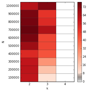
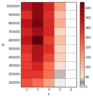
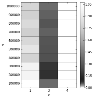
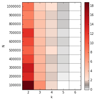
vs F, $d=2$	vs F, $d=15$	vs GUPT, $d=2$	vs GUPT, $d=15$

Figure 14: $k$-variates++ vs Forgy initialisation differentially private and GUPT. We use ratio $\uprho^{\prime}_{\phi}$ between the potential of the contender in (F-dp, GUPT) over the potential of $k$-variates++ (potentials are averaged 30 times). The more red, the better is $k$-variates++ with respect to the contender. Grey values indicate less positive outcomes for $k$-variates++; white values indicate that $k$-variates++ does not manage to find an $\epsilon^{\prime}$ larger than $\epsilon$, and thus does not manage to put smaller noise rate than in the Laplace mechanism.

$\hookrightarrow$ Comparison on synthetic domains

The synthetic datasets contain points uniformly sampled on a unit $d$-ball, in low dimension $d=2$ and higher dimension $d=15$ , we generated datasets with size in $\left\{10^{5},10^{6}\right\}$.

References

- Acharyya et al. (2013) Acharyya, S., Banerjee, A., and Boley, D. Bregman divergences and triangle inequality. In Proc. of the SIAM International Conference on Data Mining, pp. 476–484, 2013.
- Ackermann et al. (2010) Ackermann, M.-R., Lammersen, C., Märtens, M., Raupach, C., Sohler, C., and Swierkot, K. Streamkm++: A clustering algorithms for data streams. In 12th ALENEX, pp. 173–187, 2010.
- Ailon et al. (2009) Ailon, N., Jaiswal, R., and Monteleoni, C. Streaming -means approximation. In NIPS*22, pp. 10–18, 2009.
- Arthur & Vassilvitskii (2007) Arthur, D. and Vassilvitskii, S. -means++ : the advantages of careful seeding. In 19th SODA, pp. 1027 – 1035, 2007.
- Arthur et al. (2011) Arthur, D., Manthey, B., and Röglin, H. Smoothed analysis of the -means method. JACM, 58:19, 2011.
- Bahmani et al. (2012) Bahmani, B., Moseley, B., Vattani, A., Kumar, R., and Vassilvitskii, S. Scalable -means++. In 38th VLDB, pp. 622–633, 2012.
- Balcan et al. (2013) Balcan, M.-F., Ehrlich, S., and Liang, Y. Distributed -means and -median clustering on general communication topologies. In NIPS*26, pp. 1995–2003, 2013.
- Banerjee et al. (2005) Banerjee, A., Merugu, S., Dhillon, I., and Ghosh, J. Clustering with Bregman divergences. JMLR, 6:1705–1749, 2005.
- Boissonnat et al. (2010) Boissonnat, J.-D., Nielsen, F., and Nock, R. Bregman voronoi diagrams. DCG, 44(2):281–307, 2010.
- Chaudhuri et al. (2011) Chaudhuri, K., Monteleoni, C., and Sarwate, A.-D. Differentially private empirical risk minimization. JMLR, 12:1069–1109, 2011.
- Chichignoud & Lousteau (2014) Chichignoud, M. and Lousteau, S. Adaptive noisy clustering. IEEE Trans. IT, 60:7279–7292, 2014.
- Dwork & Roth (2014) Dwork, C. and Roth, A. The algorithmic foudations of differential privacy. Found. Trends in TCS, 9:211–407, 2014.
- Dwork et al. (2006) Dwork, C., McSherry, F., Nissim, K., and Smith, A. Calibrating noise to sensitivity in private data analysis. In 3rd TCC, pp. 265–284, 2006.
- Har-Peled & Mazumdar (2004) Har-Peled, S. and Mazumdar, S. On coresets for -means and -median clustering. In 37th ACM STOC, pp. 291–300, 2004.
- Hardt & Price (2014) Hardt, M. and Price, E. The noisy power method: a meta algorithm with applications. In NIPS*27, pp. 2861–2869, 2014.
- Indyk et al. (2014) Indyk, P., Mahabadi, S., Mahdian, M., and Mirrokni, V.-S. Composable core-sets for diversity and coverage maximization. In 33rd ACM PODS, pp. 100–108, 2014.
- Jegelka et al. (2009) Jegelka, S., Sra, S., and Banerjee, A. Approximation algorithms for tensor clustering. In 20th ALT, pp. 368–383, 2009.
- Kalai & Vempala (2005) Kalai, A. and Vempala, S. Efficient algorithms for online decision problems. J. Comp. Syst. Sc., pp. 291–307, 2005.
- Kohavi & Wolpert (1996) Kohavi, R. and Wolpert, D. Bias plus variance decomposition for zero-one loss functions. In 13th ICML, pp. 275–283, 1996.
- Liberty et al. (2014) Liberty, E., Sriharsha, R., and Sviridenko, M. An algorithm for online -means clustering. CoRR, abs/1412.5721, 2014.
- Liu et al. (2012) Liu, M., Vemuri, B.-C., .i Amari, S., and Nielsen, F. Shape retrieval using hierarchical total bregman soft clustering. IEEE Trans. PAMI, 34(12):2407–2419, 2012.
- McSherry (2010) McSherry, F. Privacy integrated queries: an extensible platform for privacy-preserving data analysis. Communications of the ACM, 53(9):89–97, 2010.
- Mohan et al. (2012) Mohan, P., Thakurta, A., Shi, E., Song, D., and Culler, D.-E. GUPT: privacy preserving data analysis made easy. In 38th ACM SIGMOD, pp. 349–360, 2012.
- Nielsen & Nock (2015) Nielsen, F. and Nock, R. Total Jensen divergences: definition, properties and clustering. In 40th IEEE ICASSP, pp. 2016–2020, 2015.
- Nissim et al. (2007) Nissim, K., Raskhodnikova, S., and Smith, A. Smooth sensitivity and sampling in private data analysis. In 40th ACM STOC, pp. 75–84, 2007.
- Nock et al. (2008) Nock, R., Luosto, P., and Kivinen, J. Mixed Bregman clustering with approximation guarantees. In 19th ECML, pp. 154–169, 2008.
- Nock et al. (2016) Nock, R., Nielsen, F., and Amari, S.-I. On conformal divergences and their population minimizers. IEEE Trans. IT, 62:1–12, 2016.
- Shindler et al. (2011) Shindler, M., Wong, A., and Meyerson, A. Fast and accurate -means for large datasets. In NIPS*24, pp. 2375–2383, 2011.
- von Luxburg (2010) von Luxburg, U. Clustering stability: an overview. Found. Trends in ML, 2(3):235–274, 2010.
- Wang et al. (2015) Wang, Y., Wang, Y.-X., and Singh, A. Differentially private subspace clustering. In NIPS*28, 2015.