The $UBV$ Color Evolution of Classical Novae. II. Color-Magnitude Diagram

Izumi Hachisu Department of Earth Science and Astronomy, College of Arts and Sciences, The University of Tokyo, 3-8-1 Komaba, Meguro-ku, Tokyo 153-8902, Japan hachisu@ea.c.u-tokyo.ac.jp Mariko Kato Department of Astronomy, Keio University, Hiyoshi, Kouhoku-ku, Yokohama 223-8521, Japan

Abstract

We have examined the outburst tracks of 40 novae in the color-magnitude diagram (intrinsic $B-V$ color versus absolute $V$ magnitude). After reaching the optical maximum, each nova generally evolves toward blue from the upper-right to the lower-left and then turns back toward the right. The 40 tracks are categorized into one of six templates: very fast nova V1500 Cyg; fast novae V1668 Cyg, V1974 Cyg, and LV Vul; moderately fast nova FH Ser; and very slow nova PU Vul. These templates are located from the left (blue) to the right (red) in this order, depending on the envelope mass and nova speed class. A bluer nova has a less massive envelope and faster nova speed class. In novae with multiple peaks, the track of the first decay is more red than that of the second (or third) decay, because a large part of the envelope mass had already been ejected during the first peak. Thus, our newly obtained tracks in the color-magnitude diagram provide useful information to understand the physics of classical novae. We also found that the absolute magnitude at the beginning of the nebular phase is almost similar among various novae. We are able to determine the absolute magnitude (or distance modulus) by fitting the track of a target nova to the same classification of a nova with a known distance. This method for determining nova distance has been applied to some recurrent novae and their distances have been recalculated.

Subject headings:

novae, cataclysmic variables — stars: individual (FH Ser, LV Vul, PU Vul, V1500 Cyg) — stars: winds

^†^†slugcomment: to appear in the Astrophysical Journal, Supplement Series

1. Introduction

A classical nova is a thermonuclear runaway event triggered by unstable hydrogen-burning on a mass-accreting white dwarf (WD) in a binary. After an outburst begins, the hydrogen-rich envelope expands to red-giant size and ejects mass. The nova brightens up in the optical. After maximum expansion of the pseudo-photosphere, it begins to shrink owing to mass ejection. The mass ejection process is well described by the optically thick wind theory (e.g., Kato & Hachisu, 1994; Hachisu & Kato, 2006). The optical brightness decays and subsequently, the ultra-violet (UV) emission dominates the spectrum. Finally, the super-soft X-ray emission increases. The nova outburst ends when the hydrogen shell burning is extinguished.

Several groups proposed various time-scaling laws to identify a common pattern among the nova light curves (see, e.g., Hachisu et al., 2008, for a summary). Hachisu & Kato (2006) found a similarity in the optical and near-infrared (NIR) light curves and calculated time-normalized light curves in terms of free-free emission, which are independent of the WD mass, chemical composition of the ejecta, and wavelength. They called it “the universal decline law.” This decline law was examined in a number of classical novae (Hachisu & Kato, 2007, 2009, 2010, 2015, 2016; Hachisu et al., 2006b, 2007, 2008; Kato et al., 2009; Kato & Hachisu, 2012). Based on the universal decline law, the maximum-magnitude versus rate-of-decline (MMRD) law was theoretically derived for classical novae (Hachisu & Kato, 2010, 2015, 2016). To summarize, nova optical and NIR light curves can be explained theoretically in terms of free-free emission based on the optically thick winds (Kato & Hachisu, 1994).

The evolution of colors was also studied by many researchers (see, e.g., Duerbeck & Seitter, 1979; van den Bergh & Younger, 1987; Miroshnichenko, 1988). If the optical fluxes in the $UBV$ bands are dominated by free-free emission as derived by Hachisu & Kato (2006), its color is simply estimated to be $(B-V)_{0}=+0.13$ and $(U-B)_{0}=-0.82$ for optically thin free-free ( $F_{\nu}\propto\nu^{0}$ ) emission, or to be $(B-V)_{0}=-0.03$ and $(U-B)_{0}=-0.97$ for optically thick free-free ( $F_{\nu}\propto\nu^{2/3}$ ) emission (Wright & Barlow, 1975). Here, $F_{\nu}$ is the flux at the frequency $\nu$ , $(B-V)_{0}$ and $(U-B)_{0}$ are the intrinsic colors of $B-V$ and $U-B$ , respectively. However, the nova $B-V$ color does not always stay long at these points but evolves further toward blue. Hachisu & Kato (2014, hereafter, Paper I) examined the color-color evolutions for a number of novae and identified a general course of classical nova outbursts in the $B-V$ versus $U-B$ color-color diagram. Matching the observed track of a target nova with this general course, they obtained the color excess of the nova. This is a new way to determine the color excess of a nova. A part of the extinctions thus obtained are summarized in Table 1.

In the present paper, we examine if there is also a general track of novae in the color-magnitude diagram. To obtain the intrinsic colors and absolute magnitudes of novae, we need to know the color excess (or extinction) for each nova. For this purpose, we used the results obtained in Paper I. The present paper is organized as follows. In Section 2, we examine the color-magnitude evolutions of ten well-observed novae, i.e., V1668 Cyg, LV Vul, FH Ser, PW Vul, V1500 Cyg, V1974 Cyg, PU Vul, V723 Cas, HR Del, and V5558 Sgr. Using these data, we deduce six templates of outburst tracks in the color-magnitude diagram. In Section 3, we apply these templates to 30 novae, and try to identify general trends of novae. Table 1 lists the object name, outburst year, color excess, distance modulus in the $V$ band, and distance of each nova, including our target novae. Discussion and conclusions follow in Sections 4 and 5, respectively.

Table 1Extinctions, distance moduli, and distances for selected novae

Object	Outburst	$E(B-V)$	$(m-M)_{V}$	$d$	Reference^a^a 1 - Hachisu & Kato (2014), 2 - Hachisu & Kato (2015), 3 - Hachisu & Kato (2016), 4 - present work, 5 - Kato et al. (2012), 6 - Harrison et al. (2013), 7 - Sokoloski et al. (2013).
	year			(kpc)
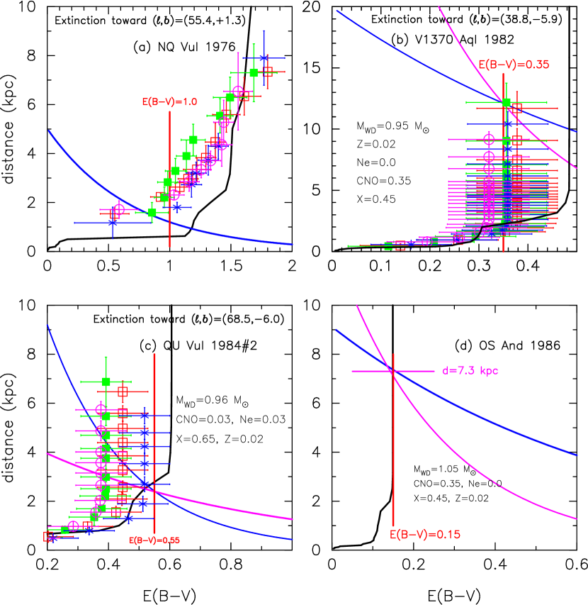
OS And	1986	0.15	14.8	7.3	1
CI Aql	2000	1.0	15.7	3.3	4
V603 Aql	1918	0.07	7.2	0.25	6
V1370 Aql	1982	0.35	16.5	12.0	4
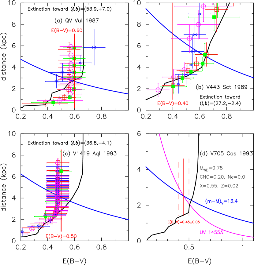
V1419 Aql	1993	0.50	14.6	4.1	1
V1493 Aql	1999#1	1.15	17.7	6.7	4
V1494 Aql	1999#2	0.50	13.1	2.0	4
V705 Cas	1993	0.45	13.4	2.5	2
V723 Cas	1995	0.35	14.0	3.85	2
V1065 Cen	2007	0.45	15.3	6.0	4
IV Cep	1971	0.65	14.7	3.4	1,4
V693 CrA	1981	0.05	14.4	7.1	3
V1500 Cyg	1975	0.45	12.3	1.5	4
V1668 Cyg	1978	0.30	14.6	5.4	3
V1974 Cyg	1992	0.30	12.2	1.8	3
V2274 Cyg	2001#1	1.35	18.7	8.0	4
V2275 Cyg	2001#2	1.05	16.3	4.1	4
V2362 Cyg	2006	0.60	15.9	6.4	4
V2467 Cyg	2007	1.40	16.2	2.4	4
V2468 Cyg	2008	0.75	15.6	4.5	4
V2491 Cyg	2008	0.23	16.5	14.0	4
HR Del	1967	0.12	10.4	1.0	4
DQ Her	1934	0.10	8.2	0.39	6
V446 Her	1960	0.40	11.7	1.23	1
V533 Her	1963	0.038	10.8	1.36	4
GQ Mus	1983	0.45	15.7	7.3	2
RS Oph	1958	0.65	12.8	1.4	1
V2615 Oph	2007	0.95	16.5	5.1	4
GK Per	1901	0.30	9.3	0.48	6
RR Pic	1925	0.04	8.7	0.52	6
V351 Pup	1991	0.45	15.1	5.5	3
T Pyx	1966	0.25	14.2	4.8	1,7
U Sco	2010	0.35	16.0	9.6	4
V745 Sco	2014	0.70	16.6	7.8	4
V1280 Sco	2007#1	0.35	11.0	0.96	4
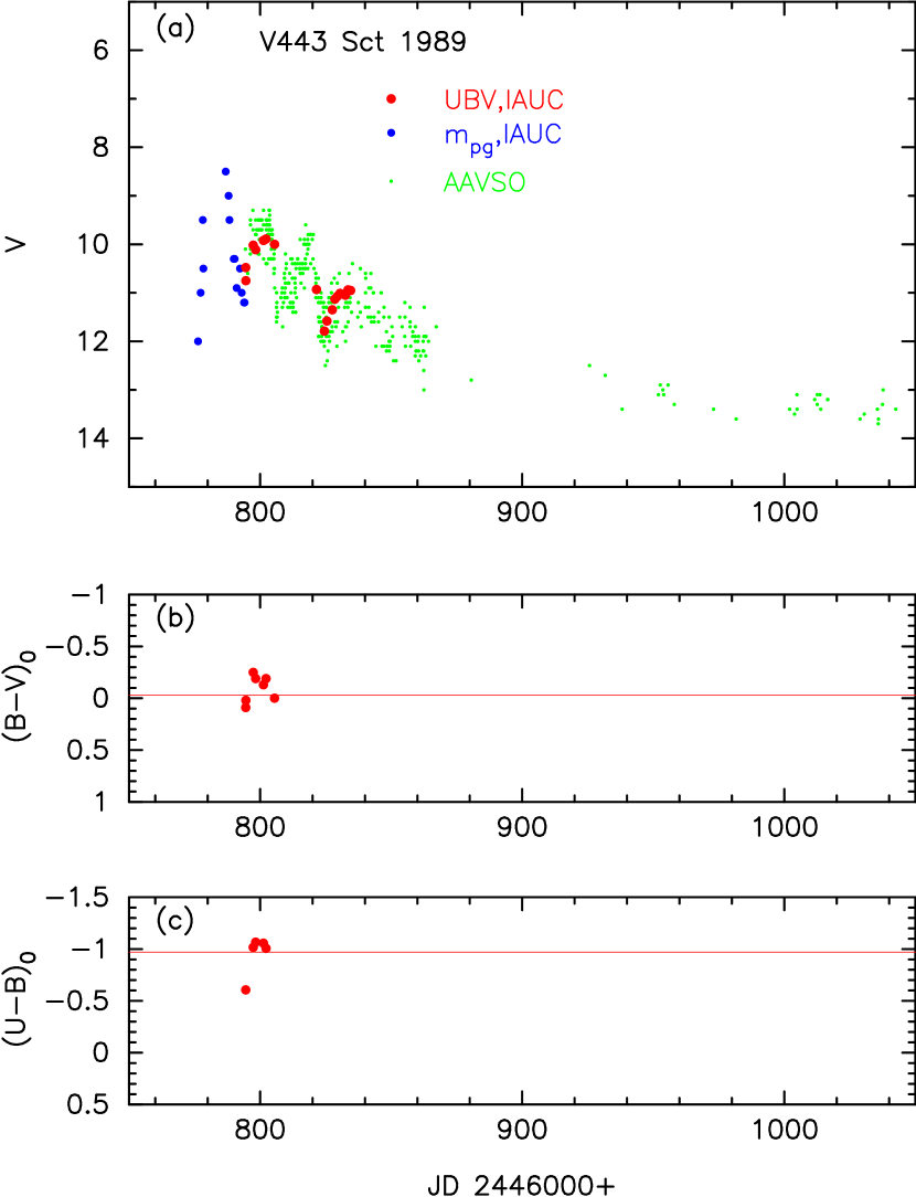
V443 Sct	1989	0.40	15.5	7.1	1
V475 Sct	2003	0.55	15.4	5.5	4
V496 Sct	2009	0.50	14.4	3.7	4
FH Ser	1970	0.60	11.7	0.93	1
V5114 Sgr	2004	0.45	16.5	10.5	1,4
V5558 Sgr	2007	0.70	13.9	2.2	1
V382 Vel	1999	0.15	11.5	1.6	3
LV Vul	1968#1	0.60	11.9	1.0	1
NQ Vul	1976	0.95	13.6	1.26	4
PU Vul	1979	0.30	14.3	4.7	5
PW Vul	1984#1	0.55	13.0	1.8	2
QU Vul	1984#2	0.55	13.6	2.4	3
QV Vul	1987	0.60	14.0	2.7	1
V458 Vul	2007#1	0.50	15.3	5.6	4

Refer to caption — Figure 1.— (a) The $V$ , $y$ , and UV 1455 Å light curves, (b) $(B-V)_{0}$ , and (c) $(U-B)_{0}$ color evolutions of V1668 Cyg. The color data are de-reddened by Equations (1) and (2) with $E(B-V)=0.30$ . See the main text for the sources of the observational data. In panel (a), the thin solid blue line denotes the model $V$ light curve of a $0.98~{}M_{\sun}$ WD with the chemical composition of CO nova 3, while the thin solid red line represents the model UV 1455 Å light curve of the same WD model, both of which are taken from Hachisu & Kato (2016). In panel (b), the $B-V$ data of Kolotilov (1980) are systematically shifted toward blue by 0.1 mag. The horizontal solid red line denotes $(B-V)_{0}=-0.03$ , which is the $B-V$ color of optically thick free-free emission. In panel (c), the $U-B$ data of Kolotilov (1980) are also systematically shifted toward blue by 0.1 mag. The horizontal solid red line denotes $(U-B)_{0}=-0.97$ , which is the $U-B$ color of optically thick free-free emission.

2. Color-magnitude Evolutions of Well-observed Novae

In this section, we study ten well-observed novae, V1668 Cyg, LV Vul, FH Ser, PW Vul, V1500 Cyg, V1974 Cyg, PU Vul, V723 Cas, HR Del, and V5558 Sgr, in this order. These ten novae were examined in detail in Paper I based on the color-color diagram. Here, we examine each nova in the color-magnitude diagram.

2.1. V1668 Cyg 1978

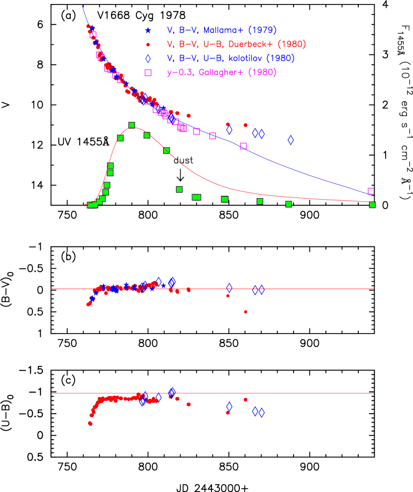
Figure 1 shows (a) the $V$ , $y$ , and UV 1455 Å light curves, (b) $(B-V)_{0}$ , and (c) $(U-B)_{0}$ color evolutions of V1668 Cyg. Here, $(B-V)_{0}$ and $(U-B)_{0}$ are the de-reddened colors of $B-V$ and $U-B$ , i.e.,

(B-V)_{0}=(B-V)-E(B-V),

(1)

(U-B)_{0}=(U-B)-0.64E(B-V),

(2)

where the factor of $0.64$ is taken from Rieke & Lebofsky (1985). The UV 1455 Å band is designed to represent continuum flux of UV light (a narrow 20 Å width band at the center of 1455Å, Cassatella et al., 2002). The $UBV$ data of V1668 Cyg are taken from Duerbeck et al. (1980) and Kolotilov (1980) whereas the $BV$ data are from Mallama & Skillman (1979) and the $y$ data are from Gallagher et al. (1980). The $V$ light curve of V1668 Cyg has $t_{2}=12.2$ and $t_{3}=24.3$ days (Mallama & Skillman, 1979). Hachisu & Kato (2016) reanalyzed the light curves of V1668 Cyg on the basis of model light curves, including the effects of both free-free emission and photospheric emission. They redetermined the reddening as $E(B-V)=0.30\pm 0.05$ and the distance modulus in the $V$ band as $\mu_{V}=(m-M)_{V}=14.6\pm 0.1$ .

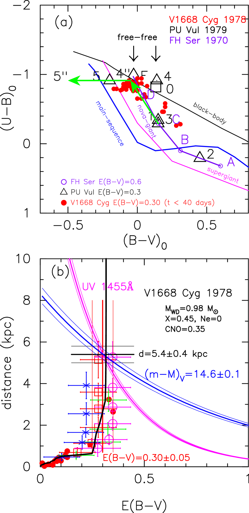
Adopting their value of $E(B-V)=0.30$ , we plot the color-color diagram of V1668 Cyg in Figure 2(a). Because the reddening of V1668 Cyg was updated to $E(B-V)=0.30$ in Hachisu & Kato (2016) from $E(B-V)=0.35$ in Paper I, we revised the color-color diagram (Figure 2(a)) and conclude that the reddening value of $E(B-V)=0.30$ is still consistent with the general tracks of novae (solid green lines).

Next, we examine the combination of the revised values of $E(B-V)=0.30$ and $\mu_{V}=(m-M)_{V}=14.6$ in the distance-reddening relation for V1668 Cyg, whose galactic coordinates are $(l,b)=(90\fdg 8373,-6\fdg 7598)$ . Figure 2(b) shows various distance-reddening relations for V1668 Cyg. Marshall et al. (2006) published a three-dimensional extinction map of our galaxy in the direction of $-100\fdg 0\leq l\leq 100\fdg 0$ and $-10\fdg 0\leq b\leq+10\fdg 0$ with grids of $\Delta l=0\fdg 25$ and $\Delta b=0\fdg 25$ , where $(l,b)$ are the galactic coordinates. Their results are shown by four directions close to V1668 Cyg. We also plot the result given by Slovak & Vogt (1979) (filled red circles). Recently, Green et al. (2015) published data for the galactic extinction map, which covers a wider range of the galactic coordinates (over three quarters of the sky) with much finer grids of 3 $\farcm$ 4 to 13 $\farcm$ 7 and a maximum distance resolution of 25%. Their values of $E(B-V)$ could have an error of 0.05 – 0.1 mag compared with other two-dimensional dust extinction maps. We added Green et al.’s distance-reddening line (the best fitted of their examples) as the thick solid black line in Figure 2(b).

We also added our results of the model light curve fits of the $V$ (solid blue lines) and UV 1455 Å (solid magenta lines) bands to Figure 2(b). These relations are calculated as follows: Figure 1(a) shows the theoretical light curve taken from Hachisu & Kato (2016), who calculated nova model light curves for various chemical compositions and WD masses based on free-free emission plus photospheric emission. The solid blue line shows the $V$ model light curve of a $0.98~{}M_{\sun}$ WD with the chemical composition of “CO nova 3” (Hachisu & Kato, 2016). Here we adopt their value $(m-M)_{V}=14.6$ for V1668 Cyg. Then, the distance-reddening relation is calculated from

(m-M)_{V}=5\log(d/{\rm 10~{}pc})+3.1E(B-V),

(3)

together with $(m-M)_{V}=14.6\pm 0.1$ . We plot Equation (3) by the blue thick solid line flanked with thin solid blue lines in Figure 2(b). Hachisu & Kato (2016) also calculated the narrow band UV 1455 Å flux (Cassatella et al., 2002) for the same WD model on the basis of blackbody emission, which is shown in Figure 1(a) by the solid red line. Fitting our model with the observed fluxes, we also obtain a distance-reddening relation

2.5\log\left(F_{\lambda}^{\rm obs}/F_{\lambda}^{\rm mod}\right)=R_{\lambda}E(B-V)+5\log\left({{d}\over{10~{}{\rm kpc}}}\right),

(4)

where $F_{\lambda}^{\rm mod}$ is the model flux at the distance of $d=10$ kpc, $F_{\lambda}^{\rm obs}$ is the observed flux, the absorption is calculated from $A_{\lambda}=R_{\lambda}E(B-V)$ , and $R_{\lambda}=8.3$ for $\lambda=1455$ Å (Seaton, 1979). For V1668 Cyg, $F_{1455}^{\rm obs}=4.0$ and $F_{1455}^{\rm mod}=11.75$ in units of $10^{-12}$ erg cm^-2 s^-1 Å^-1 at the upper bound of Figure 1(a). This distance-reddening relation is plotted by the magenta lines with a $\sim 10$ % flux 1 $\sigma$ error in Figure 2(b). All the above trends consistently cross each other at $d\approx 5.4$ kpc and $E(B-V)\approx 0.30$ as shown in Figure 2(b).

V1668 Cyg is located much below the galactic plane because its galactic coordinates are $(l,b)=(90\fdg 8373,-6\fdg 7598)$ . It is far from the galactic plane ( $-z>0.6$ kpc) and much below the galactic matter distribution (e.g., $z\sim 125$ pc, Marshall et al., 2006) for a distance of $d\sim 5.4$ kpc. Therefore, the extinction for V1668 Cyg should be close to the galactic dust extinction (two-dimensional map). The NASA/IPAC Galactic dust absorption map¹¹1http://irsa.ipac.caltech.edu/applications/DUST/, which is based on the data of Schlafly & Finkbeiner (2011), gives $E(B-V)=0.29\pm 0.02$ for V1668 Cyg. Thus, we confirmed that the adopted value of $E(B-V)=0.30$ is reasonable. Our distance and reddening estimates appear in Table 1.

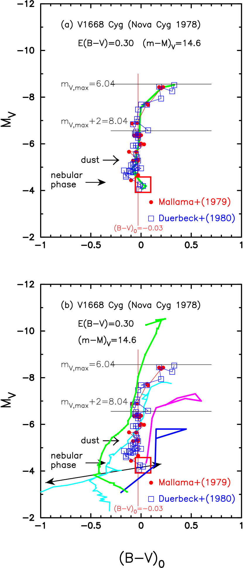
Using the new value of $E(B-V)=0.30$ together with $(m-M)_{V}=14.6$ , we plot the color-magnitude diagram of V1668 Cyg in Figure 3(a). The two horizontal solid lines indicate stages at the $V$ maximum, $m_{V,\rm max}$ , and 2 mag below the $V$ maximum, $m_{V,\rm max}+2$ . After the optical maximum ( $m_{V}\approx 6$ ), V1668 Cyg goes down almost along the line of $(B-V)_{0}=-0.03$ , which is the intrinsic $B-V$ color of optically thick free-free emission (Hachisu & Kato, 2014). This is consistent with the theoretical light curve of Figure 1(a), in which the flux of free-free emission dominates the photospheric emission. An optically thin dust shell formed at $m_{V}\sim 10.5$ (Gehrz et al., 1980) as indicated by an arrow. After that, V1668 Cyg entered the nebular phase about 4 mag below the maximum (e.g., Klare et al., 1980). It moves rightward, i.e., toward red, around/after the start of the nebular phase and then turns to the left, i.e., toward blue. The position of this turning point is denoted by the large open red square at $M_{V}=-4.19$ and $(B-V)_{0}=+0.02$ . We define a template of the color-magnitude track for V1668 Cyg by a thick solid green line in Figure 3(a). The orbital period of 3.32 hr was detected by Kałużny (1990). Table 2 lists the position ( $(B-V)_{0}$ , $M_{V}$ ) of the turning point in the color-magnitude diagram, distance modulus in the $V$ band, orbital period (if it is known), and type of the track in the color-magnitude diagram on the basis of our classification introduced later in Section 2.11.

Figure 3(b) compares the V1668 Cyg track with other well-observed novae, V1500 Cyg (thick solid green line), V1974 Cyg (thick solid cyan line), FH Ser (thick solid magenta line), and PU Vul (thick solid blue line), the data of which are taken from later sections corresponding to each nova. These novae follow a similar path but their tracks are located from left to right depending on the nova speed class, i.e., $t_{2}=2.4$ , 12.2, 17, 42, and $\gtrsim 1500$ days for V1500 Cyg, V1668 Cyg, V1974 Cyg, FH Ser, and PU Vul, respectively, except for the nebular phase. We also added a two-headed arrow, which shows Equation (5). We discuss these properties later in Section 2.12.

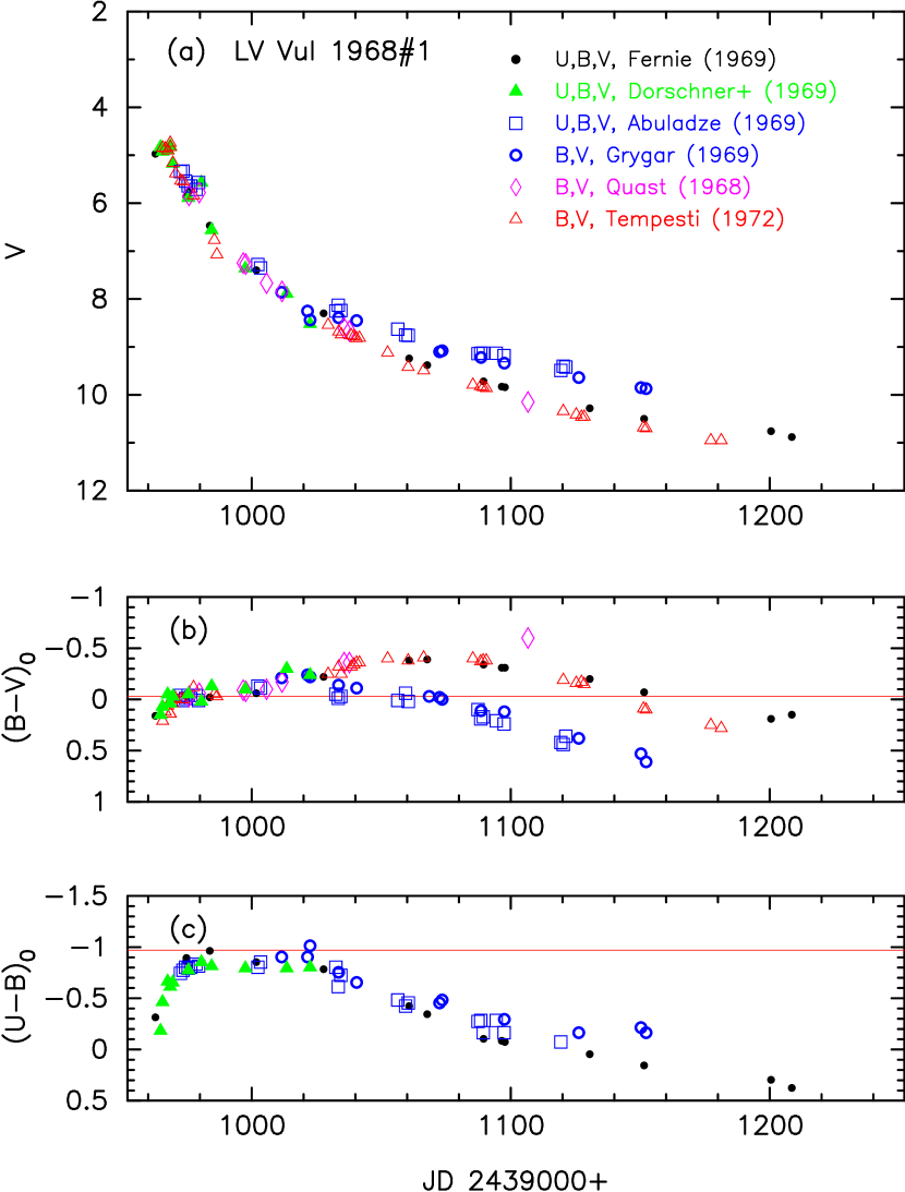
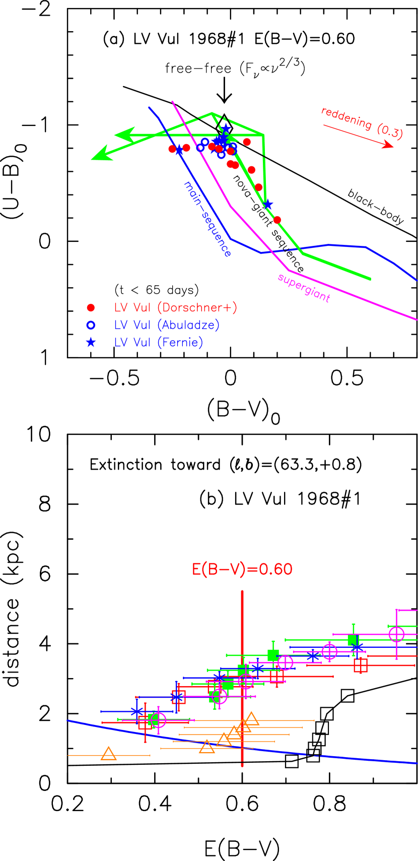
2.2. LV Vul 1968#1

The reddening for LV Vul was estimated to be $E(B-V)=0.60\pm 0.05$ by matching the observed color-color track with the general course of novae (Hachisu & Kato, 2014). Figure 4 shows the $V$ , $(B-V)_{0}$ , and $(U-B)_{0}$ evolutions of LV Vul. The $(B-V)_{0}$ and $(U-B)_{0}$ colors are de-reddened with $E(B-V)=0.60$ . The $UBV$ data are taken from Fernie (1969), Dorschner et al. (1969), Abuladze (1969), and Grygar (1969). The $BV$ data are taken from Quast (1968) and Tempesti (1972). In Figure 4(b), the $B-V$ data of Dorschner et al. (1969) are 0.05 mag redder than the other data, so we shifted them toward blue by 0.05 mag. LV Vul reached its optical maximum at $m_{V,\rm max}=4.7$ on UT 1968 April 17. The $V$ light curve of LV Vul has $t_{2}=20.2$ and $t_{3}=37$ days (Tempesti, 1972).

We plot the color-color diagram of LV Vul in Figure 5(a), using the data shown in Figure 4(b) and (c). Andrillat et al. (1986) recorded a spectrum at the pre-maximum phase and it showed a spectrum of an F-type supergiant star. Therefore, we expect that the early color evolution of LV Vul follows the nova-giant sequence in the color-color diagram. We confirm that the adopted value of $E(B-V)=0.60$ is reasonable because the observed track of LV Vul is located on the general course of novae (solid green lines) especially on the nova-giant sequence.

Hachisu & Kato (2006) found that nova light curves follow a universal decline law when free-free emission dominates the spectrum. Using the universal decline law, Hachisu & Kato (2010) derived that if two nova light curves overlap each other after one of them is squeezed/stretched by a factor of $f_{s}$ ( $t=t^{\prime}\times f_{s}$ ) in the direction of time, one nova brightness of ( $m^{\prime}_{V},~{}t^{\prime}$ ) is related to the other nova brightness of ( $m_{V},~{}t$ ) as $m_{V}=m^{\prime}_{V}+2.5\log f_{s}$ . Using this result and the calibrated nova light curves, we are able to estimate the absolute magnitude of a target nova. They called this method the “time-stretching method.”

Hachisu & Kato (2014) estimated the absolute magnitude of LV Vul as $(m-M)_{V}=11.9$ , using the time-stretching method. Then the distance is calculated to be $d=1.0$ kpc for $E(B-V)=0.60$ , which is consistent with $d=0.92\pm 0.08$ kpc obtained by Slavin et al. (1995) from the expansion parallax method. We plot the various distance-reddening relations for LV Vul, $(l,b)=(63\fdg 3024,+0\fdg 8464)$ , in Figure 5(b). Our set of $E(B-V)=0.60$ and $d=1.0$ kpc is located in a different area than the relations of both Marshall et al. (2006) and Green et al. (2015). Our result is roughly at midway between theirs. We also plot the results of Hakkila et al. (1997). Their distance-reddening relation is roughly consistent with our set of $E(B-V)=0.60$ and $d=1.0$ kpc.

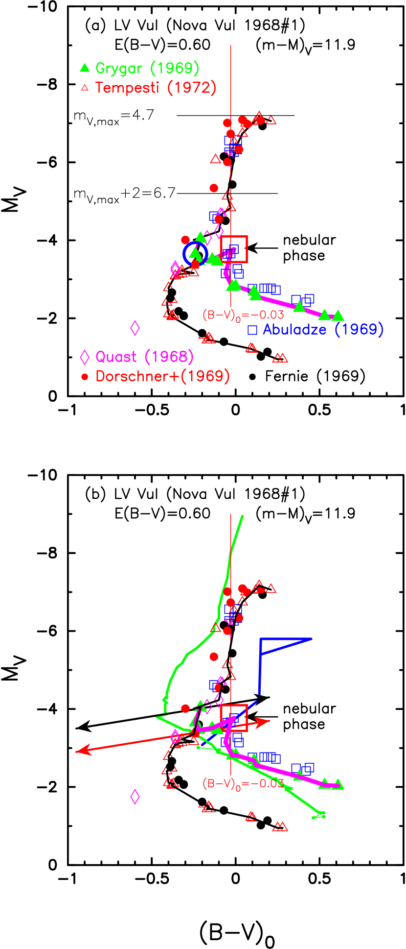
Adopting $E(B-V)=0.60$ and $(m-M)_{V}=11.9$ , we plot the color-magnitude diagram of LV Vul in Figure 6(a). After the optical maximum, LV Vul goes down almost along the line of $(B-V)_{0}=-0.03$ . This is similar to the trend in V1668 Cyg. After that, the track of LV Vul departs into two tracks at $m_{V}=8.2$ (denoted by an open blue circle at $M_{V}=8.2-11.9=-3.7$ ) in the color-magnitude diagram of Figure 6(a). This reason will be clarified below shortly after the explanation of the nebular phase.

The start of the nebular phase is identified by the first clear appearance of the nebular emission lines [O III] (or [Ne III]) stronger than the permitted lines. LV Vul had already entered the nebular phase on June 20 at $m_{V}=8.2$ (Hutchings, 1970b). Thus, we specify the onset of the nebular phase at $m_{V}=8.2$ when the track departed into two tracks (solid black and magenta lines) at the large open blue circle in Figure 6(a). The presence of two tracks is due to the strong emission lines of [O III] contributing to the blue edge of the $V$ filter. Because the response of each $V$ filter differs slightly at the shorter wavelength edge of the $V$ passband, the resultant $V$ magnitude and color index $B-V$ is significantly different among the different $V$ filters. After the nebular phase started at $m_{V}=8.2~{}(M_{V}=-3.7)$ , this difference becomes more and more significant as shown in Figure 4(a) and 4(b). Here, one group (solid magenta line) are Abuladze (1969), Dorschner et al. (1969), and Grygar (1969) and the other (solid black line) are Quast (1968), Fernie (1969), and Tempesti (1972). These two trends began to depart at $m_{V}=8.2~{}(M_{V}=-3.7)$ in the color-magnitude diagram of Figure 6(a). We also specify a turning (cusp) point at $(B-V)_{0}=-0.01$ and $M_{V}=-3.77$ (a large open red square) for the data of Abuladze (1969) as shown in Figure 6(a).

Figure 6(b) compares the track of LV Vul with those of V1500 Cyg (thick solid green line) and PU Vul (thick solid blue line) in the color-magnitude diagram. The track of LV Vul ( $t_{2}=20.2$ days) is between V1500 Cyg ( $t_{2}=2.4$ days) and PU Vul ( $t_{2}>1500$ days). The tracks are located from left to right in the order of nova speed class. This is the same trend as that of Figure 3(b), as mentioned in the previous section (Section 2.1).

The two-headed black arrow in Figure 6(b) is located 0.6 mag above the trend of the LV Vul track just after the nebular phase started. Thus, we define another line by the two-headed red arrow in the same figure. The two-headed black arrow is defined by Equation (5) and the two-headed red arrow is defined by Equation (6), both of which will be discussed later in Section 2.12. Their physical meaning will be clarified there.

2.3. FH Ser 1970

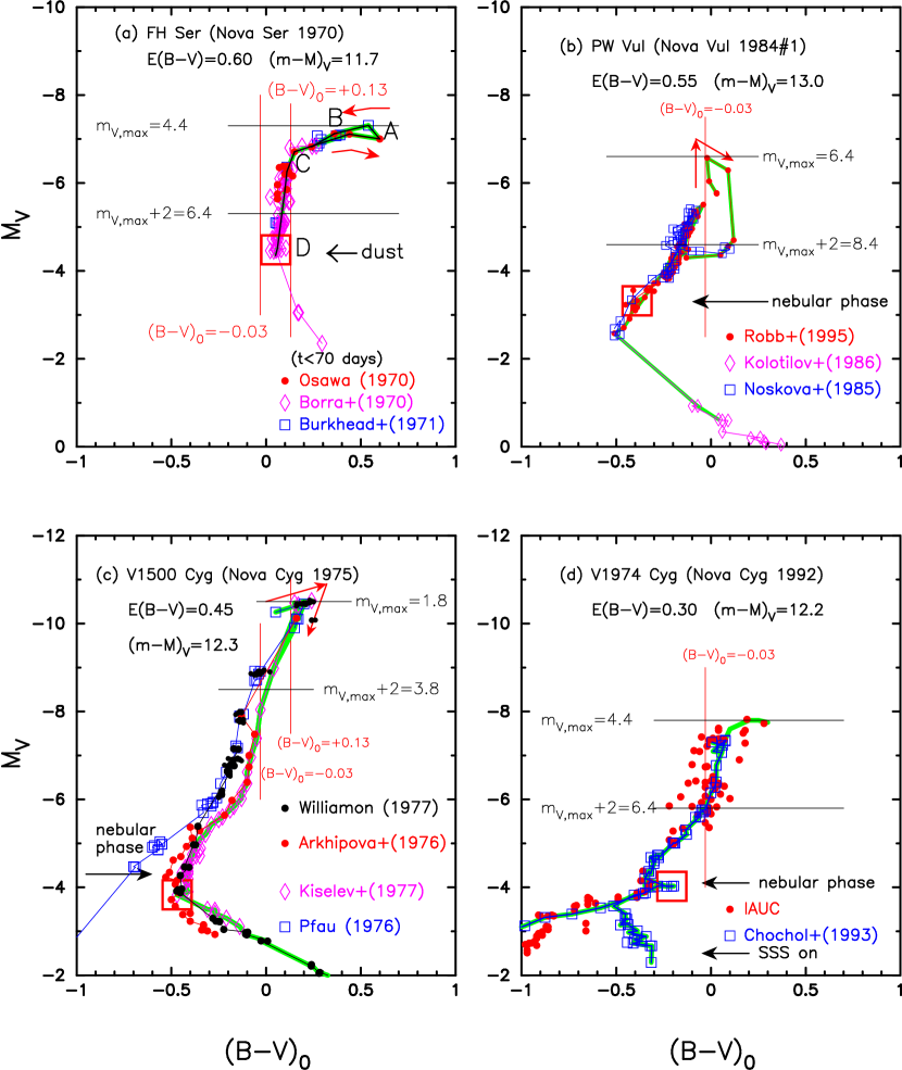
FH Ser shows a dust blackout. The $V$ light curve of FH Ser has $t_{2}=42$ and $t_{3}=59$ days (e.g., Downes & Duerbeck, 2000). The light curves of FH Ser were already analyzed in Paper I based mainly on the color-color evolution. Hachisu & Kato (2014) determined the reddening to be $E(B-V)=0.60$ and the distance modulus to be $(m-M)_{V}=11.7$ . Using the same data as those in Figure 2 of Hachisu & Kato (2014), which showed the $V$ , $(B-V)_{0}$ , and $(U-B)_{0}$ evolutions of FH Ser, we plotted the color-magnitude diagram of FH Ser in Figure 7(a). We adopted the same reddening and distance modulus as Hachisu & Kato (2014). The $UBV$ data are taken from Osawa (1970, filled red circles), Borra & Andersen (1970, open magenta diamonds), and Burkhead et al. (1971, open blue squares). The $B-V$ color of Borra & Andersen (1970) is systematically $\sim 0.2$ mag bluer than the others, while their $V$ and $U-B$ data are reasonably consistent with the others. Therefore, we shifted Borra & Andersen’s $B-V$ data 0.2 mag redder (see also Figure 2 of Hachisu & Kato, 2014). Connecting main observational points in the color-magnitude diagram, we define a template track (thick solid green line) for FH Ser in Figure 7(a).

Figure 7(a) also shows stages at the $V$ maximum, $m_{V,\rm max}$ , and 2 mag below the $V$ maximum, $m_{V,\rm max}+2$ , by the thin horizontal solid lines. FH Ser first rises in the color-magnitude diagram and then turns to the right. It goes toward red up to $(B-V)_{0}\approx+0.60$ at point A in Figure 7(a). Then, it turns back to the left, toward blue, and reaches maximum at $m_{V}=4.4~{}(M_{V}=4.4-11.7=-7.3)$ . Subsequently, it declines along the template track from point B to D through C. After point D, the nova suddenly darkened due to formation of an optically thick dust shell. We consider the start of the dust blackout (large open red square) to be $(B-V)_{0}=+0.05$ and $M_{V}=-4.48$ as shown in Figure 7(a).

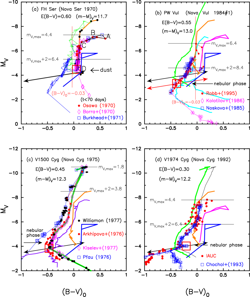
Figure 8(a) compares the color-magnitude diagram of FH Ser with those of V1668 Cyg (thin solid green lines), PW Vul (thin solid blue lines), and PU Vul (thick solid blue lines), which are analyzed in Sections 2.1, 2.4, and 2.7, respectively. The location of FH Ser ( $t_{2}=42$ days) is between those of V1668 Cyg ( $t_{2}=12.2$ days) and PU Vul ( $t_{2}\gtrsim 1500$ days). V1668 Cyg declines vertically along $(B-V)_{0}=-0.03$ (see, e.g., Hachisu & Kato, 2014, 2016), which is the color of optically thick free-free emission calculated from $F_{\nu}\propto\nu^{2/3}$ , whereas PU Vul goes down along $(B-V)_{0}=+0.13$ (see, e.g., Hachisu & Kato, 2014), the color of optically thin free-free emission calculated from $F_{\nu}\propto\nu^{0}$ . If we shift the track of V1668 Cyg toward red by $\Delta(B-V)=0.12$ mag as shown by the thick solid orange line with black points, it overlaps with that of FH Ser between $M_{V}\sim-6.5$ and $M_{V}\sim-4$ .

We examine the combination of $E(B-V)=0.60$ and $(m-M)_{V}=11.7$ in the distance-reddening relation for FH Ser, $(l,b)=(32\fdg 9090,+5\fdg 7860)$ . Figure 9(a) shows various distance-reddening relations for FH Ser. We show those given by Marshall et al. (2006), $(l,b)=(32\fdg 75,5\fdg 75)$ (open red squares), $(33\fdg 00,5\fdg 75)$ (filled green squares), $(32\fdg 75,6\fdg 00)$ (blue asterisks), and $(33\fdg 00,6\fdg 00)$ (open magenta circles). The closest one is that of the filled green squares. The solid blue line represents the relation of $(m-M)_{V}=11.7$ , crossing the trend of the filled green squares of Marshall et al. at $d\approx 0.93$ kpc and $E(B-V)\approx 0.60$ . This point is consistent with our adopted values. This figure is essentially the same as Figure 3 of Hachisu & Kato (2014), but we added the distance-reddening relation (solid black line) given by Green et al. (2015). Green et al.’s relation is located at a slightly lower position than that of Marshall et al. Considering the ambiguity of Green et al.’s relation (see Section 2.1), we may conclude that the combination of $E(B-V)=0.60$ and $d=0.93$ kpc is still reasonably consistent with these distance-reddening relations.

2.4. PW Vul 1984#1

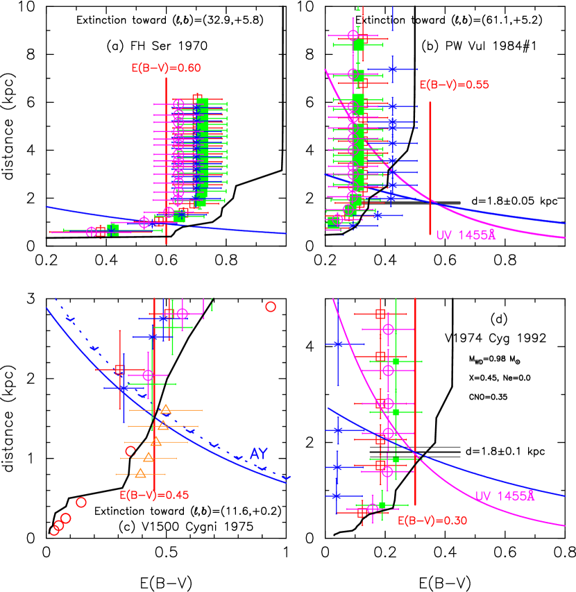
The light curves of the moderately fast nova PW Vul were studied in detail by Hachisu & Kato (2014, 2015). They determined the distance modulus to be $(m-M)_{V}=13.0$ and the reddening to be $E(B-V)=0.55$ . Figure 7(b) shows the outburst track of PW Vul in the color-magnitude diagram, the data of which are taken from Noskova et al. (1985, open blue squares), Kolotilov & Noskova (1986, open magenta diamonds), and Robb & Scarfe (1995, filled red circles). We define a template track by a thick solid green line for PW Vul almost along Robb & Scarfe’s observation in Figure 7(b).

The $V$ light curve of PW Vul shows a wavy structure in the early decline phase (see, e.g., Figure 6 of Paper I). The brightness drops to $m_{V}=8.7$ immediately after the $V$ maximum ( $m_{V,\rm max}=6.4$ ). Then it goes up to $m_{V}=7.5$ and repeats oscillations with smaller amplitudes of brightness. The smoothed $V$ light curve of PW Vul has $t_{2}=82$ and $t_{3}=126$ days (e.g., Downes & Duerbeck, 2000). PW Vul moves clockwise in the color-magnitude diagram during this first brightness drop just after the $V$ maximum, the movement direction of which is indicated by red arrows in Figure 7(b). This clockwise movement is different from the usual nova decline, like in Figure 7(a), and we will discuss it in more detail in Sections 2.10 and 2.11.

Rosino & Iijima (1987) reported that the nova entered the nebular phase at mid January 1985 (at $m_{V}=9.8$ ) as indicated in Figure 7(b). This onset corresponds to the large open red square on the track, i.e., $M_{V}=-3.32$ and $(B-V)_{0}=-0.39$ . The track of PW Vul shows a small bend globally and a tiny zigzag motion locally near this point. A possible orbital period of 5.13 hr was detected by Hacke (1987).

Figure 8(b) shows the position of PW Vul among the tracks of other novae. We also plot two-headed black and red arrows represented by Equations (5) and (6), respectively. The onset of the nebular phase (large open red square) is located on the two-headed red arrow. The track of PW Vul is very close to that of LV Vul except for the early clockwise circle. We regard PW Vul as the same type of nova as LV Vul in the color-magnitude diagram.

The five template tracks are located from left to right depending on the nova speed class, that is, $t_{2}=2.4$ , 12.2, 20.2, 42, and $\gtrsim 1500$ days for V1500 Cyg, V1668 Cyg, LV Vul, FH Ser, and PU Vul, respectively. This trend is the same as in Section 2.1. Note that the $t_{2}=82$ days of PW Vul is much longer than $t_{2}=20.2$ days of LV Vul. The reason is that the early $V$ light curve of PW Vul has a wavy structure with a large amplitude of the $V$ magnitude and the $t_{2}$ time could not represent the intrinsic nova speed class. On the other hand, other novae (V1500 Cyg, V1668 Cyg, LV Vul, FH Ser, and PU Vul) show smooth declines and their $t_{2}$ times could show their intrinsic nova speed class.

We check the combination of $E(B-V)=0.55$ and $(m-M)_{V}=13.0$ in the distance-reddening relation for PW Vul, $(l,b)=(61\fdg 0983,+5\fdg 1967)$ . Figure 9(b) shows various distance-reddening relations for PW Vul. Marshall et al.’s (2006) relations are plotted in four directions close to PW Vul: $(l,b)=(61\fdg 00,5\fdg 00)$ (open red squares), $(61\fdg 25,5\fdg 00)$ (filled green squares), $(61\fdg 00,5\fdg 25)$ (blue asterisks), and $(61\fdg 25,5\fdg 25)$ (open magenta circles). The closest one is that of blue asterisks. We also add Green et al.’s (2015) relation (thick solid black line).

Hachisu & Kato (2015) calculated model $V$ and UV 1455 Å light curves for various WD masses and chemical compositions of the hydrogen-rich envelope and obtained a best fit model for a $0.83~{}M_{\sun}$ WD with the chemical composition of CO nova 4 (see Figure 10 of Hachisu & Kato, 2015). Their UV 1455 Å fit together with Equation (4) is plotted by a solid magenta line. The $V$ light curve fit is the same as our value of $(m-M)_{V}=13.0$ . This relation is plotted by a solid blue line.

The three trends, UV 1455 Å fit, $E(B-V)=0.55$ , and $(m-M)_{V}=13.0$ , consistently cross at the point $E(B-V)\approx 0.55$ and $d\approx 1.8$ kpc, but this cross point is not consistent with the trends of Marshall et al. and Green et al. If we adopt $d=1.8$ kpc, we obtain $E(B-V)\approx 0.42$ from Marshall et al.’s relation of blue asterisks. This value is consistent with $E(B-V)=0.43\pm 0.02$ calculated from the NASA/IPAC dust map in the direction of PW Vul. Thus, our set of $E(B-V)=0.55$ and $(m-M)_{V}=13.0$ is not consistent with the trends of the 3D dust map.

Therefore, we again discuss previous reddening estimates pinpointing PW Vul. The reddening of PW Vul was estimated as $E(B-V)=A_{V}/3.1=(1.78\pm 0.05)/3.1=0.57\pm 0.02$ from the Pa $\beta$ and Pa $\gamma$ line strengths compared with H $\beta$ and H $\gamma$ line strengths by Williams et al. (1996), $E(B-V)=0.58\pm 0.06$ from the He II $\lambda 1640/\lambda 4686$ ratio, and $E(B-V)=0.55\pm 0.1$ from the interstellar absorption feature at 2200 Å both by Andreä et al. (1991), $E(B-V)=0.60\pm 0.06$ according to Saizar et al. (1991) from the He II $\lambda 1640/\lambda 4686$ ratio. The simple arithmetic mean of these four values is $E(B-V)=0.57\pm 0.1$ . The distance to PW Vul was estimated to be $d=1.8\pm 0.05$ kpc by Downes & Duerbeck (2000) from the expansion parallax method. We plot this by horizontal black lines in Figure 9(b). Then the distance modulus in the $V$ band is calculated to be $(m-M)_{V}=5\log(1800/10)+3.1\times 0.57=13.04$ . Our combination of $d=1.8$ kpc and $(m-M)_{V}=13.0$ is consistent with these estimates. The reddening trend of Marshall et al.’s blue asterisks suggests a large deviation from the other three trends by $\Delta E(B-V)\approx 0.1$ , suggesting that the reddening distribution has a patchy structure in this direction and a further deviation of $\Delta E(B-V)\sim 0.1$ may be possible. Thus, we use the set of $E(B-V)\approx 0.55$ and $d\approx 1.8$ kpc in this paper.

2.5. V1500 Cyg 1975

V1500 Cyg was identified as a neon nova by Ferland & Shields (1978a, b). The $V$ light curve shows a very rapid decline with $t_{2}=2.4$ and $t_{3}=3.7$ days (e.g., Downes & Duerbeck, 2000). The orbital period of 3.35 hr was detected by Tempesti (1975). We already analyzed the nova light curves in Paper I, and determined the reddening to be $E(B-V)=0.45\pm 0.05$ and the distance modulus to be $(m-M)_{V}=12.3\pm 0.1$ . Adopting their values of $E(B-V)=0.45$ and $(m-M)_{V}=12.3$ , we plot the color-magnitude diagram of V1500 Cyg in Figures 7(c), the data of which are taken from Arkhipova & Zaitseva (1976), Pfau (1976), Kiselev & Narizhnaia (1977), and Williamon (1977).

The spectrum energy distribution changed from blackbody emission during the first 3 days to thermal bremsstrahlung emission on day $\sim 4-5$ (Gallagher & Ney, 1976; Ennis et al., 1977). Thus, we conclude that the nova enters a free-free emission phase about 5 days after the outburst. Optically thin free-free emission ( $F_{\nu}\propto\nu^{0}$ ) yields $(B-V)_{0}=+0.13$ whereas optically thick free-free emission ( $F_{\nu}\propto\nu^{2/3}$ ) gives $(B-V)_{0}=-0.03$ , both of which are indicated in Figure 7(c).

In Figure 7(c), different observers obtained different tracks. The data of Pfau (1976) are $\sim 0.2$ mag bluer than that of the solid green line based mainly on the data of Kiselev & Narizhnaia (1977). This difference is partly attributed to slight difference in the response of each color filter which is sensitive to strong emission lines on the edge and eventually makes the nova color significantly different among the observers. We define a template track of V1500 Cyg by the thick solid green line, which is based mainly on the data taken from Kiselev & Narizhnaia (1977).

The first feature of the nebular, forbidden, lines of [O III] and [Ne III], appeared on September 8, 1975, at $m_{V}=6.1$ and their intensities steadily increased and reached that of H $\beta$ on October 12.9, at $m_{V}=7.9$ (e.g., Woszczyk et al., 1975). We specify that the nebular phase started around October 13.0–14.0, that is, $M_{V}=m_{V}-(m-M)_{V}=7.9-12.3=-4.4$ . The two tracks of Williamon (1977) and Pfau (1976) began to diverge at $M_{V}=m_{V}-(m-M)_{V}=6.1-12.3=-6.2$ as shown in Figure 7(c). This is due to the contribution of strong emission lines [O III] close to the blue edge of the $V$ filter. After the nebular phase started at $M_{V}\sim-4.4$ , this difference develops more and more. The strong emission lines of [O III] eventually made the nova color evolution turn to the right for the three cases of Williamon (1977), Arkhipova & Zaitseva (1976), and Kiselev & Narizhnaia (1977) near the cusp (or zigzag) point denoted by a large open red square. This position is $M_{V}=-3.83$ ( $m_{V}=8.5$ ) and $(B-V)_{0}=-0.47$ based on the data (filled red circles) of Arkhipova & Zaitseva (1976).

Figure 8(c) shows the position of V1500 Cyg among other well-observed novae. The track of V1500 Cyg is located on the bluest side in the color-magnitude diagram. The onset of the nebular phase (large open red square) is located on this two-headed arrow.

The distance to V1500 Cyg was discussed by many authors (see Paper I). We obtained the set of $E(B-V)=0.45$ and $(m-M)_{V}=12.3$ in Paper I. Figure 9(c) shows various distance-reddening relations toward V1500 Cyg, $(l,b)=(89\fdg 8233,-0\fdg 0720)$ . We add Marshall et al.’s (2006) relations for four directions close to V1500 Cyg, that is, $(l,b)=(89\fdg 75,0\fdg 00)$ (open red squares), $(90\fdg 00,0\fdg 00)$ (filled green squares), $(89\fdg 75,-0\fdg 25)$ (blue asterisks), and $(90\fdg 00,-0\fdg 25)$ (open magenta circles). We further add the relations of Hakkila et al. (1997) and Green et al. (2015). Green et al.’s relation gives $d=1.5$ kpc for $E(B-V)=0.45$ .

We also plot the two relations $(m-M)_{V}=12.3$ (solid blue line) and $E(B-V)=0.45$ (vertical solid red line), which are taken from Hachisu & Kato (2014). These two relations and Green et al.’s relation cross each other at the same point of $d\approx 1.5$ kpc and $E(B-V)\approx 0.45$ , consistent with the distance estimate of $d=1.5\pm 0.1$ kpc by the expansion parallax method. This strongly supports Hachisu & Kato’s (2014) set of $(m-M)_{V}=12.3$ and $E(B-V)=0.45$ .

2.6. V1974 Cyg 1992

V1974 Cyg was identified as a neon nova by Hayward et al. (1992). The $V$ light curve shows a fast decline with $t_{2}=17$ and $t_{3}=37$ days (e.g., Downes & Duerbeck, 2000). The orbital period of 1.95 hr was detected by De Young & Schmidt (1994). Paper I and Hachisu & Kato (2016) already analyzed the nova light curves on the basis of the universal decline law and determined the reddening as $E(B-V)=0.30\pm 0.05$ and the distance modulus as $(m-M)_{V}=12.2\pm 0.1$ . Adopting their values of $E(B-V)=0.30$ and $(m-M)_{V}=12.2$ , we plot the color-magnitude diagram of V1974 Cyg in Figure 7(d). The observational data are taken from Chochol et al. (1993) and IAU Circular Nos. 5455, 5457, 5459, 5460, 5463, 5467, 5475, 5479, 5482, 5487, 5490, 5520, 5526, 5537, 5552, 5571, and 5598. We define a template track of V1974 Cyg by the thick solid green line, based mainly on the data of Chochol et al. (1993).

The nova entered the nebular phase on April 20 at $m_{V}=8.1$ (Rafanelli et al., 1995), as indicated by an arrow in Figure 7(d). The position is denoted by a large open red square at $M_{V}=-4.02$ and $(B-V)_{0}=-0.21$ . This point is taken from the observational points of Chochol et al. (1993) and corresponds to a cusp on the track. We list the values at the cusp in Table 2. We add the epoch when the supersoft X-ray source (SSS) phase started at $m_{V}=9.7$ about 250 days after the outburst (Krautter et al., 1996).

Figure 8(d) compares the position of V1974 Cyg with other well-observed novae. The track of V1974 Cyg is located between those of V1500 Cyg and FH Ser. The data of V1974 Cyg taken from IAU Circulars (filled red circles) scatter slightly and their blue edge (blue side bound) coincides with the template track of V1500 Cyg whereas their red side edge almost coincides with the template track of FH Ser. We shift the track of V1500 Cyg toward red by $\Delta(B-V)=0.12$ mag and plot it by a thin solid black line, which overlaps with that of V1974 Cyg between $M_{V}=-8$ and $M_{V}=-4$ . The onset of the nebular phase (large open red square) is located on the two-headed black arrow.

Figure 9(d) shows various distance-reddening relations for V1974 Cyg, $(l,b)=(89\fdg 1338,7\fdg 8193)$ . We plot our distance modulus of $(m-M)_{V}=12.2$ by a thick solid blue line and the UV 1455 Å light curve fit by a thick solid magenta line (Hachisu & Kato, 2016). We added Chochol et al.’s distance value as $d=1.8\pm 0.1$ kpc (horizontal straight solid black line flanked by thin lines). Marshall et al.’s (2006) relations are given for $(l,b)=(89\fdg 00,7\fdg 75)$ (open red squares), $(89\fdg 25,7\fdg 75)$ (filled green squares), $(89\fdg 00,8\fdg 00)$ (blue asterisks), and $(89\fdg 25,8\fdg 00)$ (open magenta circles). We also add Green et al.’s (2015) relation by a thick solid black line. These trends almost cross at the same point of $E(B-V)\approx 0.30$ and $d\approx 1.8$ kpc. This agreement strongly supports our set of $(m-M)_{V}=12.2$ and $E(B-V)=0.30$ .

2.7. PU Vul 1979

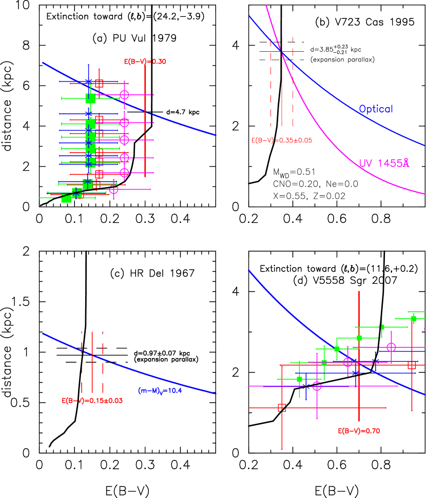
PU Vul is a symbiotic nova with an orbital period of 13.46 yr (e.g., Kato et al., 2012). Figure 10(a) shows various distance-reddening relations for PU Vul, $(l,b)=(62\fdg 5753,-8\fdg 5317)$ . Kato et al. (2012) examined the distance-reddening relation for PU Vul with several different methods and determined the reddening as $E(B-V)=0.30$ , the apparent distance modulus in the $V$ band as $(m-M)_{V}=14.3$ , and the distance as $d=4.7$ kpc. We plot these results in Figure 10(a) by the vertical solid red line, solid blue line, and horizontal black line, respectively. Hachisu & Kato (2014) reanalyzed the light curve and color-color evolution of PU Vul and reached the same conclusion, i.e., $E(B-V)=0.30$ and $(m-M)_{V}=14.3$ . The NASA/IPAC galactic dust absorption map gives $E(B-V)=0.29\pm 0.01$ in the direction toward PU Vul. We also add Marshall et al.’s (2006) and Green et al.’s (2015) distance-reddening relations to Figure 10(a). Green et al.’s trend consistently crosses our solid lines at $d=4.7$ kpc and $E(B-V)=0.30$ , which supports the values of $E(B-V)=0.30$ and $(m-M)_{V}=14.3$ .

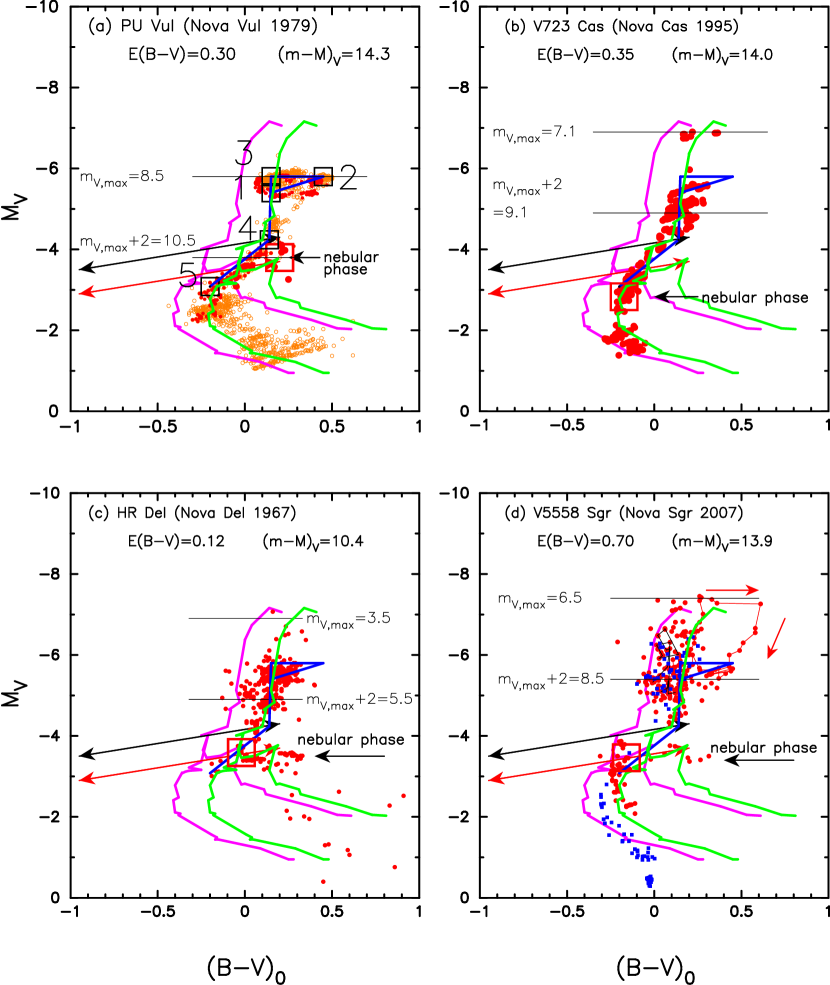
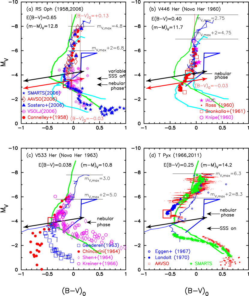
Figure 11(a) shows the color-magnitude track of PU Vul as well as the template track of LV Vul (thick solid magenta line). Here, we use $E(B-V)=0.30$ and $(m-M)_{V}=14.3$ for PU Vul. The solid green line represents the track of LV Vul, but is shifted toward red by $\Delta(B-V)=0.2$ . The data of the small open orange circles are taken from Shugarov et al. (2012). The other data of small filled red circles are taken from various sources but are the same as in Figures 16 and 17 of Paper I. We define a template track of PU Vul by a thick solid blue line. The numbers 1 – 5 attached to large open black squares on the solid blue line correspond to the stages 1 – 5 of PU Vul as defined in Figure 15 of Paper I. The figure also shows the stages at the $V$ maximum, $m_{V,\rm max}$ , and 2 mag below the $V$ maximum, $m_{V,\rm max}+2$ , by thin horizontal solid lines. It is remarkable that the green shifted LV Vul track almost coincides with the PU Vul track except for the flat optical peak of PU Vul (see Figure 15 of Paper I for the $V$ light curve of PU Vul).

Vogel & Nussbaumer (1992) reported that a distinct nebular spectrum emerged between September 1989 ( $m_{V}\approx 10.4$ , $M_{V}\approx-3.9$ ) and November 1990 ( $m_{V}\approx 10.6$ , $M_{V}\approx-3.7$ ). We consider this to be the nova entering the nebular phase at $m_{V}\approx 10.5$ ( $M_{V}\approx-3.8$ ), which is denoted by an arrow in Figure 11(a). Here we specify this onset point by a large open red square at $(B-V)_{0}=+0.20$ and $M_{V}=-3.80$ . The onset of the nebular phase (large open red square) is located on the two-headed red arrow. This position accidentally coincides with the onset point of the nebular phase on the green shifted LV Vul track as shown in Figure 6(a).

2.8. V723 Cas 1995

V723 Cas is a very slow nova with an orbital period of 16.64 hr (Goranskij et al., 2000). Figure 10(b) shows various distance-reddening relations for V723 Cas, $(l,b)=(124\fdg 9606,-8\fdg 8068)$ . The NASA/IPAC galactic dust absorption map gives $E(B-V)=0.34\pm 0.01$ in the direction toward V723 Cas. We plot the distance-reddening relation given by Green et al. (2015) by a solid black line, the apparent distance modulus in the $V$ band of $(m-M)_{V}=14.0$ (Hachisu & Kato, 2015) by a solid blue line, the reddening of $E(B-V)=0.35\pm 0.05$ from Paper I by a vertical solid red line flanked with dashed red lines, the distance of $d=3.85^{+0.23}_{-0.21}$ kpc from the expansion parallax method (Lyke & Campbell, 2009) by a horizontal solid black line flanked with dashed lines, and the UV 1455 Å model light curve fit (Hachisu & Kato, 2015) by a solid magenta line. All these trends cross each other at $E(B-V)\approx 0.35$ and $d\approx 3.85$ kpc. Therefore, we adopt $E(B-V)=0.35$ and $(m-M)_{V}=5\log(3850/10)+3.1\times 0.35=14.0$ for V723 Cas after Hachisu & Kato (2015).

Figure 11(b) shows the color-magnitude track of V723 Cas. The data of V723 Cas are taken from Chochol & Pribulla (1997). The solid green line represents the LV Vul track shifted toward red by $\Delta(B-V)=0.2$ . The PU Vul and green shifted LV Vul tracks are remarkably similar to that of V723 Cas except for the flaring pulses around optical maximum of $M_{V}=-7$ to $-6$ . See Figures 19, 20, and 21 of Paper I for the $V$ light curve and color curves.

The onset of the nebular phase was detected by Iijima (2006) between May 30 and July 1, 1997, at $m_{V}\approx 11.3$ , as shown in Figure 11(b). We specify the point $(B-V)_{0}=-0.17$ and $M_{V}=-2.83$ from the observational data in Figure 11(b), and denote it by a large open red square. The start of the nebular phase is slightly below the line of the two-headed red arrow.

2.9. HR Del 1967

HR Del is a very slow nova with an orbital period of 5.14 hr (Bruch, 1982; Kürster & Barwig, 1988). The light curve shape is very similar to that of V723 Cas and V5558 Sgr (see, e.g., Figures 19, 20, and 21 of Paper I). Figure 10(c) shows several distance-reddening relations, the apparent distance modulus in the $V$ band of $(m-M)_{V}=10.4$ (Hachisu & Kato, 2015), the reddening of $E(B-V)=0.15\pm 0.03$ (Verbunt, 1987), and the distance of $d=0.97\pm 0.07$ kpc (Harman & O’Brien, 2003). We also add Green et al.’s (2015) relation. All the trends consistently cross at $E(B-V)\approx 0.12$ and $d\approx 1.0$ kpc. The NASA/IPAC galactic dust absorption map also gives $E(B-V)=0.112\pm 0.006$ in the direction toward HR Del, $(l,b)=(63\fdg 4304,-13\fdg 9721)$ . Therefore, we adopt $E(B-V)=0.12$ and $(m-M)_{V}=10.4$ for HR Del.

Figure 11(c) shows the color-magnitude track of HR Del. The data of HR Del are taken from O’Connell (1968), Mannery (1970), Barnes & Evans (1970), and Onderlička & Vetešník (1968). The track of HR Del is very similar to that of PU Vul except for the flaring pulses around the optical peak of HR Del. The track of HR Del also follows the green LV Vul track shifted toward red by $\Delta(B-V)=0.2$ .

The start of the nebular phase was identified by Hutchings (1970a) at $(B-V)_{0}=-0.02$ and $M_{V}=-3.59$ , which is indicated by a large open red square in Figure 11(c). The track of HR Del departs into two branches at this point, depending on the different filter responses of various observers, just as for LV Vul. One of them turns to the right (toward red) when the nebular phase started. This departing point accidentally coincides with that of the green shifted LV Vul track. The start of nebular phase is almost on the line of the two-headed red arrow.

2.10. V5558 Sgr 2007

V5558 Sgr is a very slow nova. Its light curve shape is very similar to that of V723 Cas and HR Del (see, e.g., Figures 19, 20, and 21 of Paper I). Figure 10(d) shows various distance-reddening relations for V5558 Sgr, $(l,b)=(11\fdg 6107,-0\fdg 2067)$ . This figure is the same as Figure 24 of Paper I, but we added Green et al.’s (2015) relation. All the trends consistently cross at $E(B-V)\approx 0.70$ and $d\approx 2.2$ kpc. Therefore, we adopt $E(B-V)=0.70$ and $(m-M)_{V}=13.9$ , the same values as in Paper I.

Figure 11(d) shows the color-magnitude track of V5558 Sgr. The data of V5558 Sgr are taken from the archives of the American Association of Variable Star Observers (AAVSO, filled red circles), the Variable Star Observers League of Japan (VSOLJ, filled red circles), and SMARTS²²2http://www.astro.sunysb.edu/fwalter/SMARTS/NovaAtlas/ (Walter et al., 2012) (filled blue squares).

The track of V5558 Sgr is very similar to that of PU Vul, except for the flaring pulses around the optical peak. We connect the track of V5558 Sgr by a thin solid red line during the first flaring pulse around the optical maximum. Also, we connect the track during the second flaring pulse by a thin solid black line. The first flaring pulse shows a clockwise movement in the color-magnitude diagram. This clockwise behavior is very similar to that of PW Vul in Figure 7(b). This clockwise movement, however, is very large in V5558 Sgr. It rises vertically along $(B-V)_{0}\sim 0.2$ up to the maximum brightness ( $m_{V}\sim 6.5$ , $M_{V}\sim-7.4$ ), then turns to the right (toward red) up to $(B-V)_{0}\sim 0.6$ , and then goes down to $M_{V}\sim-5.8$ , coinciding with the flat maximum brightness of PU Vul. This large clockwise circular movement in the color-magnitude diagram is very different from the usual tracks of novae such as FH Ser and LV Vul. The track of the second flaring pulse follows that of the first flaring pulse in the rising phase but does not go toward red. It loops on the blue side of the first flaring pulse. The third and fourth flaring pulses follow the second flaring pulse and these tracks almost overlap the track of the second flaring pulse. They are very similar to the loop of PW Vul in Figure 7(b).

The start of the nebular phase was identified by Poggiani (2012) at $(B-V)_{0}=-0.16$ and $M_{V}=-3.46$ , which is denoted by a large open red square in Figure 11(d). The track of V5558 Sgr departs into two branches at this point, depending on the different filter responses of various observers just as in LV Vul and HR Del. One of them turns to the right (toward red) when the nebular phase started. The start of the nebular phase is located on the line of the two-headed red arrow.

2.11. Categorization of color-magnitude tracks

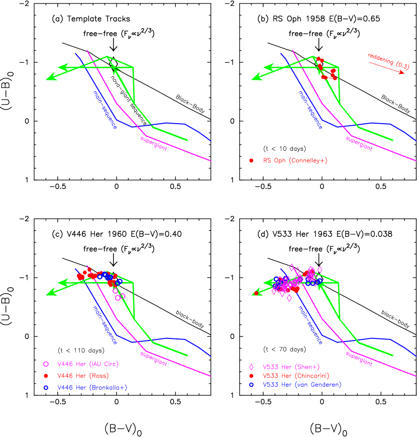
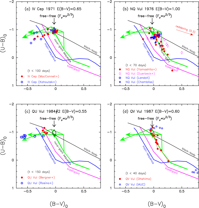
It is clear that there is no single track common to all novae in the color-magnitude diagram. This is in contrast to the general track in the color-color diagram. In Paper I, we found that, in the color-color diagram, novae generally go down along the nova-giant sequence in the pre-maximum phase and then come back after the optical maximum as shown in Figure 2(a) (see also Figures 4 and 8 of Paper I). Fast novae tend to have short excursions and slow novae tend to have long journeys to their peaks along the nova-giant sequence.

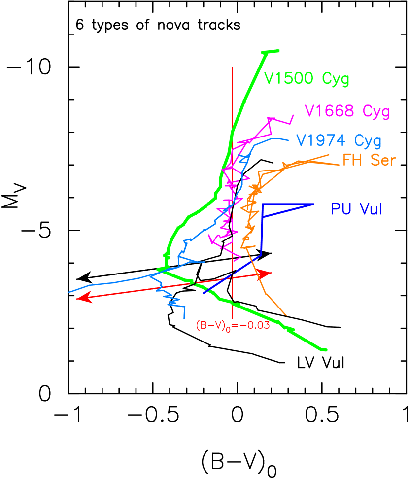
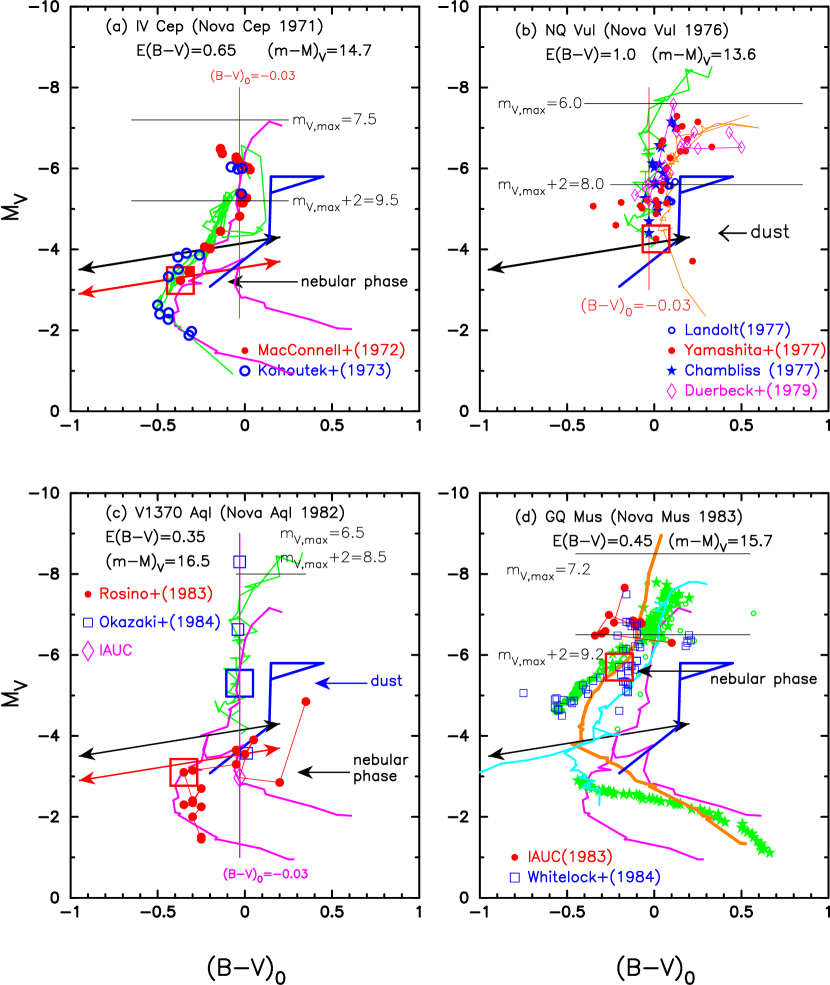
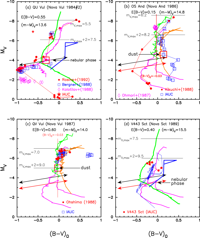
Figure 12 collects the templates of the color-magnitude diagrams for the very fast nova V1500 Cyg, fast novae V1668 Cyg, V1974 Cyg, and LV Vul, moderately fast nova FH Ser, and symbiotic (very slow) nova PU Vul. Because we excluded novae such as PW Vul, which shows oscillatory behavior around the optical peak, all these six novae show smooth declines from their optical peaks. The behaviors of these six novae in the color-magnitude diagram are summarized as follows: (1) After the optical peak, each nova generally evolves toward blue from the upper-right to the lower-left along similar but different tracks. (2) Each track is located from the left (blue) to right (red) depending on the nova speed class, i.e., $t_{2}=2.4$ , 12.2, 17, 20.4, 42, $\gtrsim 1500$ days for V1500 Cyg, V1668 Cyg, V1974 Cyg, LV Vul, FH Ser, and PU Vul, respectively. Thus, we propose six templates of smooth decline nova tracks, i.e., V1500 Cyg, V1668 Cyg, V1974 Cyg, LV Vul, FH Ser, and PU Vul.

In the previous subsections, we examined the behaviors of ten novae in the color-magnitude diagram. The LV Vul track almost overlaps that of PW Vul except for the early pulse (a loop). The track of PU Vul almost overlaps those of V723 Cas, HR Del, and V5558 Sgr except for the early pulses (loops). We may call PW Vul a LV Vul type track because the track of PW Vul is very close to the template of LV Vul. We also call V723 Cas, HR Del, and V5558 Sgr PU Vul type tracks. Thus, we define six types of nova tracks in the color-magnitude diagram, i.e., the V1500 Cyg, V1668 Cyg, V1974 Cyg, LV Vul, FH Ser, and PU Vul types.

These six template novae are further grouped into three families by their similarities. The track of V1500 Cyg overlaps that of V1974 Cyg if we shift it by $\Delta(B-V)=0.12$ mag toward red, as shown in Figure 8(d). V1668 Cyg shows a shallow dust blackout while FH Ser does a deep dust blackout. The track of V1668 Cyg is $\Delta(B-V)=0.12$ mag bluer than that of FH Ser, as shown in Figure 8(a). The track of LV Vul (PW Vul) almost overlaps those of PU Vul, V723 Cas, HR Del, and V5558 Sgr, if we shift it by $\Delta(B-V)=0.2$ mag toward red. Thus, we may categorize these ten novae into three families, i.e., V1500 Cyg, V1668 Cyg, and LV Vul families. The V1500 Cyg family includes V1500 Cyg and V1974 Cyg. The V1668 Cyg family includes V1668 Cyg and FH Ser and the LV Vul family includes LV Vul, PW Vul, PU Vul, V723 Cas, HR Del, and V5558 Sgr.

2.12. Characteristic properties of color-magnitude tracks

If optically thick free-free emission ( $F_{\nu}\propto\nu^{2/3}$ ) dominates the spectrum of a nova, its color should be $(B-V)_{0}=-0.03$ (Paper I), the color of which is indicated by a vertical thin solid red line in Figure 12. If the spectrum is of optically thin free-free emission ( $F_{\nu}\propto\nu^{0}$ ), its color is $(B-V)_{0}=+0.13$ (not shown in Figure 12). V1668 Cyg and LV Vul almost follows the line of $(B-V)_{0}=-0.03$ while V1500 Cyg and V1974 Cyg across this line and move further toward blue. This is due to emission line effects (see Figure 10 and discussion of Paper I). In the later phase, these novae turn to the right (toward red) due to the contribution of [O III] lines to the blue edge of the $V$ filter. Therefore, this excursion toward red could be prominent in the nebular phase. We have already marked the beginning of the nebular phase in each figure. For V1500 Cyg and V1974 Cyg, the start of the nebular phase agrees with the clear cusp in the color-magnitude track as indicated by the large open red squares. For V1668 Cyg, we also found a cusp (not clear, but a slight cusp) on the track as shown in Figure 3. For LV Vul, we found that the track departs into two branches at the onset of nebular phase, depending on the different response of each $V$ filter, especially on the blue edge of the response function. For the other novae, we already specify the onset of the nebular phase on their tracks if it was detected and reported in the literature.

In this way, we found that there is a special feature like a cusp, bifurcation, or sharp turning point on the track near the onset of nebular phase. Such a cusp (sharp turning point) appears at $M_{V}\approx-4$ for the three fast novae, V1668 Cyg, V1500 Cyg, and V1974 Cyg. An inflection appears also at $M_{V}\approx-4$ for the symbiotic novae PU Vul, and slow novae V723 Cas and PW Vul. We found that the positions of these cusps/inflections are located on the lines described by

M_{V}=-0.7(B-V)_{0}-4.17\pm 0.1~{}(\mbox{two-headed black arrow}).

(5)

This line is plotted in Figure 12 by the two-headed black arrow, which is obtained simply by connecting the inflection of PU Vul and the turning point of V1500 Cyg. The $1\sigma$ error of 0.1 mag comes from our entire analysis of the color-magnitude diagrams for 13 novae, which will be discussed later from Section 4.2.

For LV Vul, HR Del, and V5558 Sgr, on the other hand, the start of the nebular phase is close to the line of the two-headed red arrow in Figure 12, i.e.,

M_{V}=-0.7(B-V)_{0}-3.57\pm 0.2~{}(\mbox{two-headed red arrow}).

(6)

This line is 0.6 mag below the line of the two-headed black arrow. The $1\sigma$ error of 0.2 mag comes from our entire analysis of the color-magnitude diagrams for 11 novae, which will be discussed later from Section 4.2. These two lines are empirically determined, so we do not have a theoretical justification yet.

If the positions of cusps/inflections are always located on Equation (5) or (6), we are able to estimate the absolute magnitudes of novae by placing the observed cusp/inflection on the line of Equation (5) or (6). This could be a new method for obtaining the absolute magnitude of novae.

Table 2Start of nebular phase or dust formation in the color-magnitude diagram

Object	Outburst	$(B-V)_{0}$	$M_{V}$	$(m-M)_{V}$	$P_{\rm orb}$	Type^a^aNova tracks are categorized into six types, depending on the shape and position of the track in the color-magnitude diagram, i.e., V1500 Cyg, V1668 Cyg, V1974 Cyg, LV Vul, FH Ser, and PU Vul.	Comment^b^b“dust” indicates a dust formation nova, “recurrent” a recurrent nova, “Ne nova” a neon nova, “2nd max” a nova showing a single secondary maximum like V2362 Cyg, “transition oscillation” a nova showing a transition oscillation like GK Per, “multiple peaks” means a nova with multiple-peaks like V5558 Sgr, and “super bright” a super bright nova (della Valle, 1991).
	year				(hr)
OS And	1986	( $+0.14$ )^c^cnumbers in parenthesis show the position in the color-magnitude diagram where dust blackout starts.	( $-4.59$ )	14.8	—	V1668 Cyg	dust
CI Aql	2000	$-0.52$	$-3.84$	15.7	14.8	V1500 Cyg	recurrent
V1370 Aql	1982	$-0.35$	$-3.10$	16.5	—	LV Vul	dust, Ne nova
V1419 Aql	1993	( $-0.13$ )	( $-3.85$ )	14.6	—	V1668 Cyg	dust
V1493 Aql	1999#1	$-0.35$	$-3.78$	17.7	3.74	V1974 Cyg	2nd max
V1494 Aql	1999#2	—	—	13.1	3.23	V1500 Cyg	transition oscillation
V705 Cas	1993	( $-0.20$ )	( $-4.09$ )	13.4	5.47	V1668 Cyg	dust
V723 Cas	1996	$-0.17$	$-2.83$	14.0	16.6	PU Vul	multiple peaks
V1065 Cen	2007	$-0.35$	$-3.42$	15.3	—	LV Vul	dust, Ne nova
IV Cep	1971	$-0.37$	$-3.23$	14.7	—	LV Vul
V1500 Cyg	1975	$-0.47$	$-3.83$	12.3	3.35	V1500 Cyg	super bright, Ne nova
V1668 Cyg	1978	$+0.02$	$-4.19$	14.6	3.32	V1668 Cyg	dust
V1974 Cyg	1992	$-0.21$	$-4.02$	12.2	1.95	V1974 Cyg	Ne nova
V2274 Cyg	2001#1	—	—	18.7	—	V1668 Cyg	dust
V2275 Cyg	2001#2	—	—	16.3	7.55	V1500 Cyg
V2362 Cyg	2006	$-0.51$	$-3.83$	15.9	1.58	V1500 Cyg	2nd max
V2467 Cyg	2007	$-0.53$	$-3.88$	16.2	3.83	V1974 Cyg	transition oscillation
V2468 Cyg	2008	$-0.38$	$-3.80$	15.6	3.49	V1500 Cyg
V2491 Cyg	2008	$-0.51$	$-3.97$	16.5	—	V1500 Cyg	2nd max
HR Del	1967	$-0.02$	$-3.59$	10.4	5.14	PU Vul	multiple peaks
V446 Her	1960	$-0.13$	$-4.05$	11.7	4.97	V1668 Cyg
V533 Her	1963	$-0.40$	$-3.97$	10.8	3.53	V1974 Cyg
GQ Mus	1983	$-0.20$	$-5.70$	15.7	1.43	V1500 Cyg
RS Oph	1958	$-0.12$	$-3.29$	12.8	$1.1\times 10^{4}$	LV Vul	recurrent
V2615 Oph	2007	( $-0.06$ )	( $-4.58$ )	16.5	6.54	FH Ser	dust
T Pyx	1966	$-0.56$	$-4.59$	14.2	1.83	V1500 Cyg	recurrent
U Sco	2010	$-0.64$	$-3.72$	16.0	29.5	V1500 Cyg	recurrent
V745 Sco	2014	—	—	16.6	—	LV Vul	recurrent
V1280 Sco	2007#1	( $+0.01$ )	( $-5.70$ )	11.0	—	FH Ser	dust
V443 Sct	1989	—	—	15.5	—	LV Vul
V475 Sct	2003	( $-0.15$ )	( $-3.80$ )	15.4	—	V1668 Cyg	dust
V496 Sct	2009	$-0.35$	$-3.26$	14.4	—	LV Vul	dust
FH Ser	1970	$(+0.05)$	$(-4.48)$	11.7	—	FH Ser	dust
V5114 Sgr	2004	$-0.50$	$-3.92$	16.5	—	V1974 Cyg	transition oscillation
V5558 Sgr	2007	$-0.16$	$-3.46$	13.9	—	PU Vul	multiple peaks
V382 Vel	1999	$-0.29$	$-4.04$	11.5	3.51	V1974 Cyg	Ne nova
LV Vul	1968#1	$-0.01$	$-3.77$	11.9	—	LV Vul
NQ Vul	1976	( $+0.01$ )	( $-4.26$ )	13.6	—	FH Ser	dust
PU Vul	1979	$+0.20$	$-3.80$	14.3	$1.18\times 10^{5}$	PU Vul
PW Vul	1984#1	$-0.39$	$-3.32$	13.0	5.13	LV Vul
QU Vul	1984#2	$-0.31$	$-4.01$	13.6	2.68	V1974 Cyg	Ne nova
QV Vul	1987	( $-0.03$ )	( $-5.00$ )	14.0	—	FH Ser	dust
V458 Vul	2007#1	—	—	15.3	1.63	PU Vul	multiple peaks

3. Color-magnitude Diagrams for Various Novae

In this section, we further examine various novae in the color-magnitude diagram. We have collected data from the literature for as many novae as possible that have a sufficient number of data points (usually more than a few tens). We classify these 30 nova tracks into the previously discussed six types, i.e., V1500 Cyg, V1668 Cyg, V1974 Cyg, FH Ser, LV Vul, and PU Vul, and discuss their physical properties in the color-magnitude diagram. These 30 novae are examined in the order of discovery.

3.1. RS Oph (1958,1985,2006)

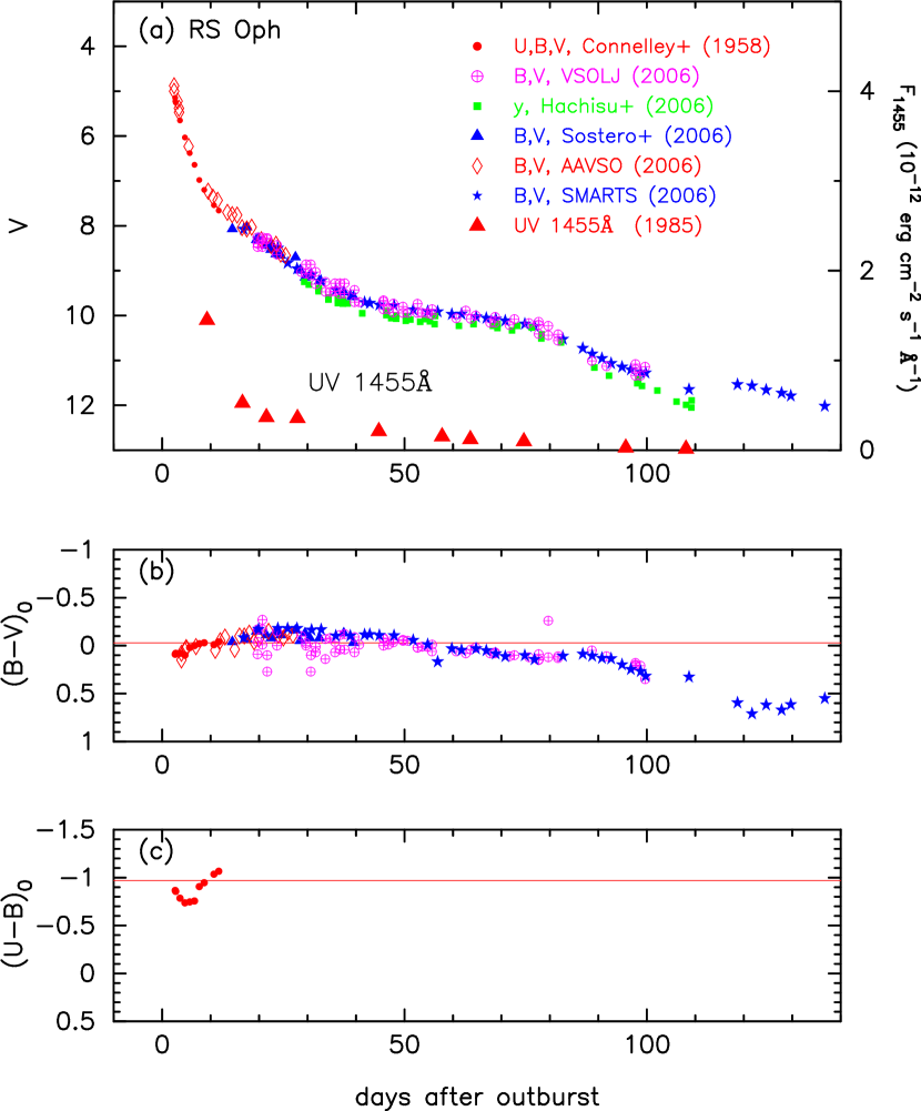
RS Oph is a recurrent nova with six recorded outbursts in 1898, 1933, 1958, 1967, 1985, and 2006. The orbital period of 456 days was obtained by Fekel et al. (2000). Figure 13 shows the $V$ , $(B-V)_{0}$ , and $(U-B)_{0}$ evolutions of RS Oph. The observed data of RS Oph are taken from Connelley & Sandage (1958) (filled red circles) for the 1958 outburst, and AAVSO (open red diamonds), VSOLJ (encircled magenta pluses), SMARTS (blue stars), Sostero & Guido (2006a, b), Sostero et al. (2006c) (filled blue triangles), and Hachisu et al. (2008b) (filled green squares: data are tabulated only in arXiv:0807.1240) for the 2006 outburst. The $V$ light curve declined with $t_{2}=6.8$ and $t_{3}=14$ days (Schaefer, 2010). In panel (b) of Figure 13, the $B-V$ data of the 2006 outburst are systematically 0.1 mag redder than those of the 1958 outburst (Connelley & Sandage, 1958), so we shifted the $B-V$ data of the 2006 outburst by 0.1 mag up (toward blue) to match them with the $B-V$ data of Connelley & Sandage (1958). The $B-V$ data of SMARTS are shifted by 0.05 mag down (toward red), however.

In Paper I, we determined the color excess as $E(B-V)=0.65\pm 0.05$ and the distance modulus as $(m-M)_{V}=12.8\pm 0.2$ on the basis of the general track in the color-color diagram and the time-stretching method, respectively. Assuming that $E(B-V)=0.65$ , we plot the color-color evolution of RS Oph (1958) in Figure 14(b). This color-color track of RS Oph is the same as that in Figure 42 of Paper I, but we reanalyze the data along the color evolution in Figure 13 and confirmed that the color excess is $E(B-V)=0.65\pm 0.05$ by matching the color-color track (filled red circles) with the general course of novae (green lines) in Figure 14(a).

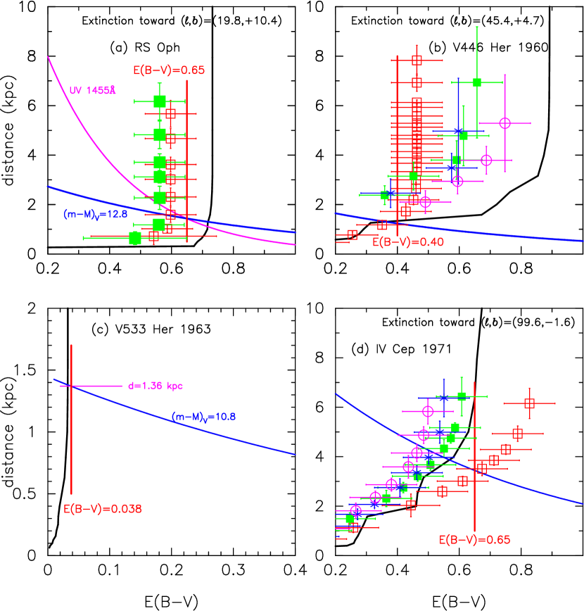
The distance to RS Oph was already discussed in Paper I. We plot various distance-reddening relations in Figure 15(a). This figure is the same as Figure 34(a) of Paper I, but we added Green et al.’s (2015) relation (solid black line). Three lines of $(m-M)_{V}=12.8$ , UV 1455 Å fit, and $E(B-V)=0.65$ cross consistently at $d\approx 1.4$ kpc. The cross point is midway between Marshall et al.’s (2006) and Green et al.’s (2015) relations. Thus, we confirmed the values in Paper I, i.e., $(m-M)_{V}=12.8$ , $E(B-V)=0.65$ , and $d\approx 1.4$ kpc.

Figure 16(a) shows the color-magnitude diagram of RS Oph. The track is very similar to that of V1668 Cyg in the early phase, but turns to the right and follows the right side of the LV Vul track in the later phase. The start of the nebular phase was identified from the 1985 outburst observed by Rosino & Iijima (1987) as shown in Figure 16(a). We specify the point as $(B-V)_{0}=-0.12$ and $M_{V}=-3.29$ with a large open red square in the figure. The starting point of the nebular phase is on the two-headed red arrow, so we identify RS Oph as an LV Vul type rather than a V1668 Cyg type in the color magnitude diagram as listed in Table 2. We add the epoch when the variable SSS phase started at $m_{V}=9.1$ , about 30 days after the outburst (Hachisu et al., 2008c; Osborne et al., 2011). The epoch, when the stable SSS phase started at $m_{V}=9.6$ , about 45 days after the outburst, is coincident with the start of the nebular phase. The track of RS Oph follows the line of $(B-V)_{0}=-0.03$ in the early phase, being consistent with optically thick free-free emission ( $F_{\nu}\propto\nu^{2/3}$ ). After the stable SSS phase started, it jumps to $(B-V)_{0}=+0.13$ and stays there for a while (between $M_{V}=-2.7$ and $M_{V}=-1.7$ ), being consistent with the optically thin free-free emission ( $F_{\nu}\propto\nu^{0}$ ). When the stable SSS phase started, the ejecta had already become optically thin. This agreement supports our adopted values of $E(B-V)=0.65$ .

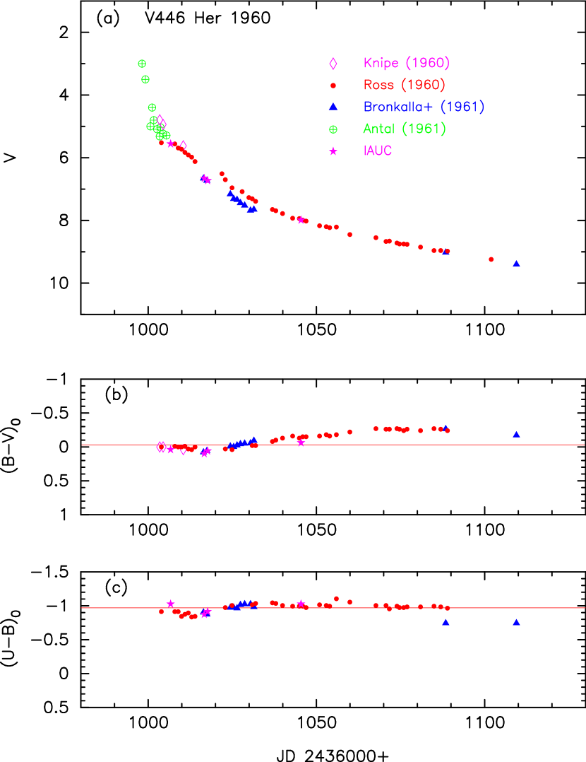
3.2. V446 Her 1960

Figure 17 shows the $V$ , $(B-V)_{0}$ , and $(U-B)_{0}$ evolutions of V446 Her. These light curve data are the same as those in Figure 42 of Paper I, but we reanalyzed the data as mentioned below. The data are taken from Antal (1961), Bronkalla & Notni (1961), Knipe (1960), Ross (1960), and IAU Circular No.1730. The orbital period of 4.97 hr was detected by Thorstensen & Taylor (2000). The $B-V$ data of the IAU Circular, Knipe (1960), and Bronkalla & Notni (1961) are systematically 0.1 mag redder than those of Ross (1960), so we shift them by 0.1 mag toward blue. As a result, the $B-V$ color curve becomes smooth as shown in Figure 17(b). We also shift the $U-B$ data of the IAU Circular and Bronkalla & Notni (1961) by 0.1 mag toward blue, so the $U-B$ color curve also becomes smooth as shown in Figure 17(c).

In Paper I, we determined the color excess as $E(B-V)=0.40\pm 0.05$ on the basis of the general track in the color-color diagram and the distance modulus as $(m-M)_{V}=11.7\pm 0.2$ by the time-stretching method. The reanalyzed data gives a consistent matching with the general tracks of novae in the color-color diagram of V446 Her as shown in Figure 14(c) for the same reddening value of $E(B-V)=0.40$ as in Paper I. We also plot various distance-reddening relations for V446 Her, $(l,b)=(45\fdg 4092,+4\fdg 7075)$ , in Figure 15(b). This figure is the same as Figure 34(b) of Paper I, but we added Green et al.’s (2015) relation (solid black line). The lines cross consistently at the point of $E(B-V)=0.40$ and $d=1.23$ kpc. Thus, we confirmed the values of Paper I, i.e., $E(B-V)=0.40$ , $(m-M)_{V}=11.7$ , and $d=1.2$ kpc.

Using $E(B-V)=0.40$ and $(m-M)_{V}=11.7$ , we plot the color-magnitude diagram of V446 Her in Figure 16(b). We identified the start of the nebular phase as $\sim 40$ days after the outburst from Figure 11 of Meinel (1963), at which the forbidden lines of [O III] surpassed the permitted lines. This epoch corresponds to $m_{V}=7.6$ ( $M_{V}=-4.1$ ) as shown in Figure 16(b). We assign the start of the nebular phase to the observational point $M_{V}=-4.05$ and $(B-V)_{0}=-0.13$ , denoted by a large open red square in Figure 16(b). The track of V446 Her goes almost vertically down along the line of $(B-V)_{0}=-0.03$ similarly to V1668 Cyg in the early phase, and turns to the left (toward blue) near the onset of nebular phase (large open red square), almost on the two-headed black arrow. Then the track turns to the right (toward red) below the two-headed red arrow. Because the start of the nebular phase is located on the two-headed black arrow, we regard V446 Her as a V1668 Cyg type in the color-magnitude diagram as listed in Table 2.

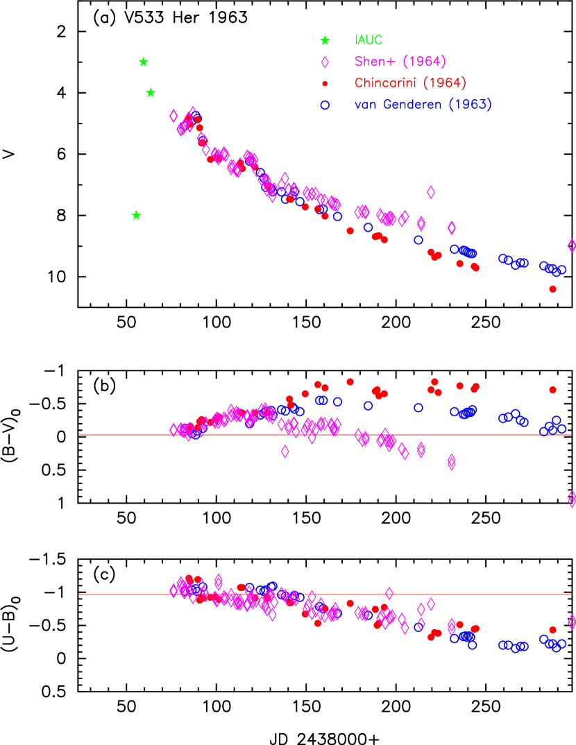
3.3. V533 Her 1963

Figure 18 shows the $V$ , $(B-V)_{0}$ , and $(U-B)_{0}$ evolutions of V533 Her, where the $UBV$ data are taken from van Genderen (1963), Chincarini (1964), and Shen et al. (1964). The orbital period of 3.53 hr was obtained by Thorstensen & Taylor (2000). The data of this figure is the same as those in Figure 41 of Paper I, but we reanalyzed the data as mentioned below. The $U-B$ data of Chincarini (1964) and van Genderen (1963) are systematically 0.3 mag redder than those of Shen et al. (1964), so we shifted them up (toward blue) by 0.3 mag in Figure 18(c).

In Paper I, we determined the color excess as $E(B-V)=0.05\pm 0.05$ on the basis of the general track in the color-color diagram, and the distance modulus as $(m-M)_{V}=10.8\pm 0.2$ ³³3It should be noted that $(m-M)_{V}=11.1$ in Table 2 of Paper I is a typographical error. by the time-stretching method (see Paper I for other estimates of reddening and distance). The NASA/IPAC galactic dust absorption map gives $E(B-V)=0.038\pm 0.002$ in the direction toward V533 Her, $(l,b)=(69\fdg 1887,+24\fdg 2733)$ . Here we adopt this smaller value of $E(B-V)=0.038$ and we plot the color-color diagram of V533 Her in Figure 14(d), resulting in a better matching with the general tracks of novae.

We plot three distance-reddening relations in Figure 15(c). The lines of $(m-M)_{V}=10.8$ and $E(B-V)=0.038$ cross at $d=1.36$ kpc, so we adopt $d=1.36$ kpc as the distance to V533 Her. The distance was estimated also by Cohen (1985) to be $d\sim 1.32$ kpc from the expansion parallax method together with the nebular expansion velocity of $v_{\rm exp}=1050$ km s^-1. Gill & O’Brien (2000) obtained $d=1.25\pm 0.30$ kpc together with $v_{\rm exp}=850\pm 150$ km s^-1. Our distance of $d=1.36$ kpc is consistent with the both values given by Cohen (1985) and Gill & O’Brien (2000). Green et al.’s (2015) distance-reddening relation is also consistent with the value of $E(B-V)=0.038$ .

Adopting $E(B-V)=0.038$ and $(m-M)_{V}=10.8$ , we plot the color-magnitude diagram in Figure 16(c). We added the $BV$ data (open magenta circles) of Kreiner et al. (1966). The nebular phase started around UT 1963 April 19 at $m_{V}=7.2$ (Chincarini & Rosino, 1964). After that, these three tracks branch off and diverge. In the nebular phase, the [O III] emission lines dominate the spectrum at the blue edge of the $V$ filter. Because the response of each $V$ filter is slightly different at the blue edge, the [O III] emission lines make a large difference in the $V$ magnitude among the observers. This can be seen clearly in Figures 3, 4, and 5 of Kreiner et al. (1966), in which the $V$ magnitude of each observer started to branch off after UT 1963 April 10 (JD 2438129.5), while the $B$ magnitude was essentially the same among the observers. This is also shown clearly in Figure 18(a) and 18(b). In the color-magnitude diagram, there is a sharp (cusp) turning point on the data of Shen et al. (1964) at $M_{V}=-3.97$ and $(B-V)_{0}=-0.40$ . We identify V533 Her as a V1974 Cyg type in the color-magnitude diagram as listed in Table 2.

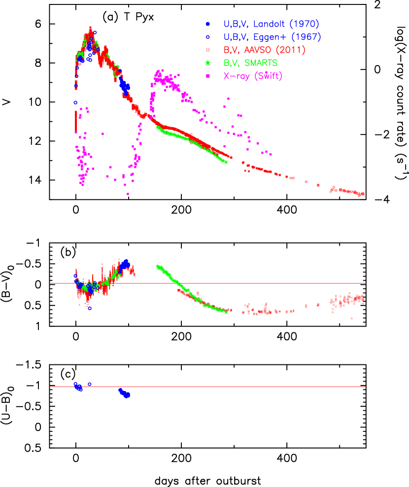
3.4. T Pyx (1966,2011)

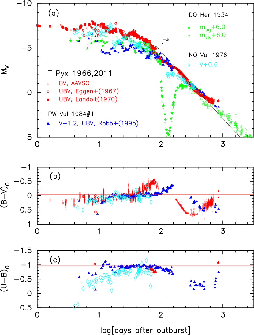
T Pyx is a recurrent nova with six recorded outbursts in 1890, 1902, 1920, 1944, 1966, and 2011. The orbital period of 1.83 hr was obtained by Uthas et al. (2010). Figure 19 shows the $V$ , $(B-V)_{0}$ , and $(U-B)_{0}$ evolutions of the 1966 and 2011 outbursts, where the $UBV$ data are taken from Eggen et al. (1967) and Landolt (1970) and the $BV$ data are taken from the SMARTS and AAVSO archives. We also added the X-ray light curve of T Pyx taken from the Swift web page⁴⁴4http://www.swift.ac.uk/ (Evans et al., 2009).

We adopt the distance of $4.8$ kpc after Sokoloski et al. (2013) and the extinction of $E(B-V)=0.25$ from Paper I (see Paper I for other estimates of the reddening and distance). Then, the distance modulus is $(m-M)_{V}=14.2$ for $E(B-V)=0.25$ and $d=4.8$ kpc. Figure 20 compares four light curves of the novae, T Pyx, DQ Her, PW Vul, and NQ Vul. The timescales of these four novae are almost the same except the early fluctuations in the optical maximum phase. The light curves of these four novae almost overlap each other in the later decline phase and decline as $t^{-3}$ (thin solid black line) except for the period of dust blackout of DQ Her, where $t$ is the time after the outburst. We obtained the following relation among them:

$\displaystyle(m-M)_{V,\rm T~{}Pyx}$	$\displaystyle=$	$\displaystyle 14.2$	(7)
	$\displaystyle=$	$\displaystyle(m-M+\Delta V)_{V,\rm DQ~{}Her}$	(8)
	$\displaystyle=$	$\displaystyle 8.2+(+6.0)=14.2$	(9)
	$\displaystyle=$	$\displaystyle(m-M+\Delta V)_{V,\rm PW~{}Vul}$	(10)
	$\displaystyle=$	$\displaystyle 13.0+(+1.2)=14.2$	(11)
	$\displaystyle=$	$\displaystyle(m-M+\Delta V)_{V,\rm NQ~{}Vul}$	(12)
	$\displaystyle=$	$\displaystyle 13.6+(+0.6)=14.2,$	(13)

where $\Delta V$ is the difference between the $V$ light curve of T Pyx and that of a target nova. We shift the optical light curve of DQ Her down by $\Delta V=6.0$ mag, that of PW Vul down by $\Delta V=1.2$ mag, and that of NQ Vul down by $\Delta V=0.6$ mag against that of T Pyx. The distance of DQ Her was obtained with the trigonometric parallax method to be $d=386^{+33}_{-29}$ pc (Harrison et al., 2013). Adopting $A_{V}=3.1\times E(B-V)=0.31$ (Verbunt, 1987), we obtain the distance modulus of DQ Her as $(m-M)_{V}=8.24\pm 0.18$ . Thus, we use $(m-M)_{V,\rm DQ~{}Her}=8.2$ . We have already obtained $(m-M)_{V,\rm PW~{}Vul}=13.0$ in Section 2.4, and $(m-M)_{V,\rm NQ~{}Vul}=13.6$ in Section 3.6. The relations in Equation (13) strongly suggest that the overlapping region of $t^{-3}$ law has almost the same absolute brightness among novae having similar timescales, although the peak absolute brightnesses are different.

Using $(m-M)_{V}=14.2$ and $E(B-V)=0.25$ , we plot the color-magnitude diagram of T Pyx in Figure 16(d), where the data are taken from Landolt (1970) for the 1966 outburst and from the SMARTS and AAVSO archives for the 2011 outburst. The nebular phase started around UT 1967 March 12, at $m_{V}\sim 9.6$ (Catchpole, 1969), corresponding to the turning point of the track, denoted by a large open red square at $M_{V}=-4.59$ and $(B-V)_{0}=-0.56$ . The track of T Pyx is located near that of V1974 Cyg in the early phase, and turns gradually to the left (toward blue) over the track of V1500 Cyg, and then suddenly turns to the right (toward red) near the starting point of the nebular phase. We add the epoch when the SSS phase started at $m_{V}=10.8$ about 120 days after the outburst (Chomiuk et al., 2014). We identify T Pyx as a V1500 Cyg type in the color-magnitude diagram as tabulated in Table 2.

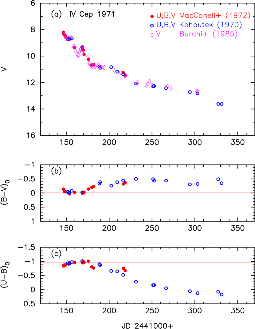
3.5. IV Cep 1971

Figure 21 shows the $V$ , $(B-V)_{0}$ , and $(U-B)_{0}$ evolutions of IV Cep. The $UBV$ data of IV Cep are taken from MacConnell & Thomas (1972) and Kohoutek & Klawitter (1973). The $V$ data are taken from Burchi & D’Ambrosio (1985). IV Cep is a fast nova with $t_{2}=25$ and $t_{3}=42$ days (e.g. Kohoutek & Klawitter, 1973). In Paper I, we determined $E(B-V)=0.70\pm 0.05$ from fitting in the color-color diagram, and $(m-M)_{V}=14.7\pm 0.2$ by the time-stretching method (see Paper I for other estimates of reddening and distance). We reanalyzed the same data and redetermined the reddening as $E(B-V)=0.65\pm 0.05$ , because, for $E(B-V)=0.65$ , more color-color data of IV Cep are concentrated on the general track (especially on the open diamond) in the color-color diagram of Figure 22(a). Then, the distance is calculated to be $d=3.4$ kpc for $E(B-V)=0.65$ .

We reanalyzed the distance-reddening relation with this new value of $E(B-V)=0.65$ as shown in Figure 15(d). The data of this figure are the same as those in Figure 34(d) of Paper I, but we added the distance-reddening relation (solid black line) given by Green et al. (2015). Because Marshall et al.’s $(l,b)=(99\fdg 5,-1\fdg 5)$ , open red squares, is closest to the position of IV Cep, $(l,b)=(99\fdg 6137,-1\fdg 6381)$ , the three trends of distance-reddening relations, i.e., Marshall et al.’s data, $E(B-V)=0.65$ , and $(m-M)_{V}=14.7$ , cross each other at $E(B-V)\approx 0.65$ and $d\approx 3.4$ kpc. Thus, we adopt $E(B-V)=0.65$ , $(m-M)_{V}=14.7$ , and $d=3.4$ kpc.

Using $E(B-V)=0.65$ and $(m-M)_{V}=14.7$ , we plot the color-magnitude diagram of IV Cep in Figure 23(a). The track almost follows that of PW Vul and LV Vul. Thus, we regard IV Cep as an LV Vul type in the color-magnitude diagram as listed in Table 2. Strong emission lines of [O III] appeared between UT 1971 September 12 and 22 (Rosino, 1975), which is an indication of the nebular phase. We identify the start of the nebular phase at $(B-V)_{0}=-0.37$ and $M_{V}=-3.23$ , denoted by a large open red square in Figure 23(a). This starting point is located on the line of two-headed red arrow.

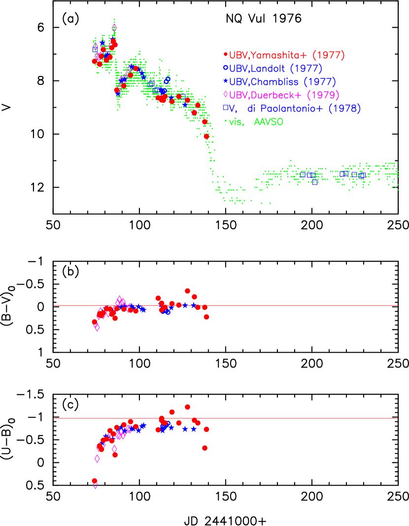
3.6. NQ Vul 1976

NQ Vul belongs to the dust blackout type novae like FH Ser. Figure 24 shows the $V$ , $(B-V)_{0}$ , and $(U-B)_{0}$ evolutions of NQ Vul, where the $UBV$ data are taken from Yamashita et al. (1977), Landolt (1977), Chambliss (1977), and Duerbeck & Seitter (1979), and the $V$ and visual magnitudes are from di Paolantonio & Patriarca (1978) and the AAVSO archive, respectively. The data of this figure are the same as those in Figure 43 of Paper I, but we reanalyzed them as mentioned below. The $B-V$ colors of Duerbeck & Seitter (1979) are systematically bluer by 0.05 mag and of Yamashita et al. (1977) are redder by 0.05 mag than the other data, so that we shift them down by 0.05 mag and up by 0.05 mag, respectively. The $U-B$ colors of Duerbeck & Seitter (1979) and Yamashita et al. (1977) are systematically redder by 0.1 and bluer by 0.1 mag than the other data, so we shift them up by 0.1 mag and down by 0.1 mag, respectively. Using these color data, we fit the color-color evolution of NQ Vul with the general track of novae and obtain $E(B-V)=1.0\pm 0.05$ as shown in Figure 22(b). We reanalyzed the color data but obtained the same result as that in Paper I.

Figure 25(a) shows various distance-reddening relations toward NQ Vul, $(l,b)=(55\fdg 3552,+1\fdg 2899)$ . The data are the same as those in Figure 35(a) of Paper I, but we add Green et al.’s (2015) relation. Our lines $(m-M)_{V}=13.6$ and $E(B-V)=1.0$ cross at the point $d=1.26$ kpc and the cross point is midway between the distance reddening relations of Marshall et al. (2006) and Green et al. (2015). Thus, we confirmed the same values as in Paper I.

Using $(m-M)_{V}=13.6$ and $E(B-V)=1.0$ , we plot the color-magnitude diagram of NQ Vul in Figure 23(b). The track of NQ Vul is located closely to that of FH Ser (solid orange lines), although the data are scattered. The large variation in the early phase data is partly owing to a few pulses on the $V$ light curve in the pre-maximum phase. We can see two small brightenings before the optical maximum in Figure 24(a). The color-magnitude data obtained by Duerbeck & Seitter (1979), which are connected by a thin solid magenta line, show two clockwise movements that correspond to the two pulses before the optical maximum in Figure 23(b). The first clockwise looping is close to the track of FH Ser. The second clockwise movement departs from the track of FH Ser and then approaches the track of V1668 Cyg. Then, the track of NQ Vul reaches its peak and goes down along between the tracks of V1668 Cyg and FH Ser after the optical maximum. The color of the track became bluer after a considerable part of the envelope mass was ejected during these early pulses. This strongly suggests that the bluer the nova color is the smaller the envelope mass is. We regard NQ Vul as a FH Ser type in the color-magnitude diagram as listed in Table 2. The start of the dust blackout is denoted by a large open red square in Figure 23(b) at $(B-V)_{0}=+0.01$ and $M_{V}=-4.26$ .

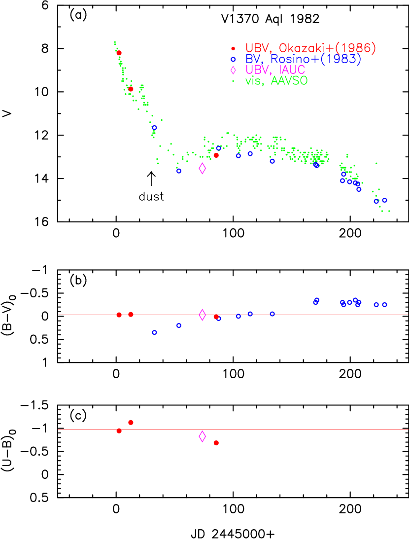
3.7. V1370 Aql 1982

V1370 Aql also shows a dust blackout, but its depth is much shallower than those of FH Ser and NQ Vul. Figure 26 depicts the $V$ and visual, $(B-V)_{0}$ , and $(U-B)_{0}$ evolutions of V1370 Aql, where the $UBV$ data are very limited. We found only the data of Okazaki & Yamasaki (1986) and IAU circular No. 3689 for the $UBV$ data and Rosino et al. (1983) for the $BV$ data in addition to the visual magnitudes from the AAVSO archive. The $V$ light curve has $t_{2}=8$ and $t_{3}=13$ days (e.g., Williams & Longmore, 1984). V1370 Aql was identified as a neon nova by Snijders et al. (1987).

In Paper I, we determined the color excess as $E(B-V)=0.35\pm 0.05$ from the color-color diagram fit, and the distance modulus as $(m-M)_{V}=15.2\pm 0.2$ by the time-stretching method relative to the distance modulus of V1668 Cyg (see Paper I for other estimates of reddening and distance). After that, Hachisu & Kato (2016) revised the distance modulus of V1668 Cyg including the photospheric emission in addition to the free-free emission. Therefore, we redetermine the distance modulus of V1370 Aql based on the new estimate of the distance modulus of V1668 Cyg (see also Section 2.1).

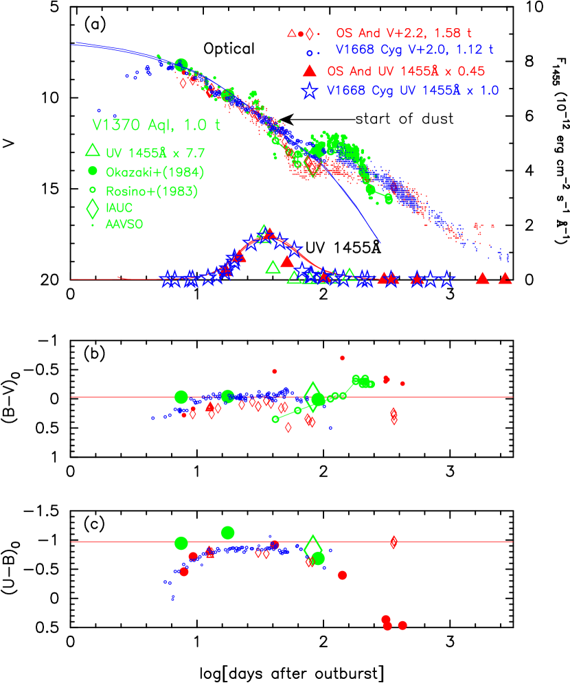
Figure 27 shows a comparison of V1370 Aql with V1668 Cyg and OS And. We adopt the stretching factor as $f_{s}=1.12$ and 1.58 for V1668 Cyg and OS And against V1370 Aql, respectively. These three nova light curves overlap each other. Then, the brightness difference is $\Delta V=2.0$ mag for V1668 Cyg and $\Delta V=2.2$ mag for OS And against that of V1370 Aql. Using the time-stretching method (see Section 2.2 for a short explanation of the time-stretching method), we obtain the distance modulus of V1370 Aql as

$\displaystyle(m-M)_{V,\rm V1370~{}Aql}$	$\displaystyle=$	$\displaystyle(m-M+\Delta V)_{V,\rm V1668~{}Cyg}-2.5\log 1.12$	(14)
	$\displaystyle=$	$\displaystyle 14.6+2.0-0.12=16.48$	(15)
	$\displaystyle=$	$\displaystyle(m-M+\Delta V)_{V,\rm OS~{}And}-2.5\log 1.58$	(16)
	$\displaystyle=$	$\displaystyle 14.8+2.2-0.50=16.50,$	(17)

where we use $(m-M)_{V,\rm V1668~{}Cyg}=14.6$ from Sections 2.1 and $(m-M)_{V,\rm OS~{}And}=14.8$ from Sections 3.10. We adopt $(m-M)_{V,\rm V1370~{}Aql}=16.5$ . Then, the distance is calculated to be $d=12$ kpc for $E(B-V)=0.35$ .

Hachisu & Kato (2016) calculated the absolute magnitudes of model light curves of novae for various sets of chemical compositions. Adopting their chemical composition of CO nova 3, we obtained a best fit $V$ (thin solid blue line) and UV 1455 Å (thin solid magenta line) light curve model for a $0.95~{}M_{\sun}$ WD and plotted them in Figure 27(a). The fitting of the $V$ light curve gives a distance modulus of $(m-M)_{V}=16.5$ , being consistent with that obtained from the time-stretching method mentioned above. Therefore, we plot the distance-reddening relations of the $V$ light curve fit calculated from Equation (3) together with $(m-M)_{V}=16.5$ (solid blue line) and the UV 1455 Å light curve fitting calculated from Equation (4) (solid magenta line) in Figure 25(b). We added other distance-reddening relations for V1370 Aql, $(l,b)=(38\fdg 8126,-5\fdg 9465)$ , in Figure 25(b), that is, the relations given by Marshall et al. (2006) and Green et al. (2015). The three trends of the distance-reddening relations, i.e., Marshall et al.’s, and two distance moduli in the $V$ and UV 1455 Å band, cross each other at $E(B-V)\approx 0.35$ and $d\approx 12$ kpc, being consistent with our estimates for V1370 Aql. Green et al.’s (2015) relation deviates largely from our value of $E(B-V)\approx 0.35$ .

Using $E(B-V)=0.35$ and $(m-M)_{V}=16.5$ , we plot the color-magnitude diagram for V1370 Aql in Figure 23(c). The peak $V$ magnitude reaches as bright as $M_{V}=m_{V}-(m-M)_{V}=6.5-16.5=-10$ . We plot the starting position of the dust blackout in the color-magnitude diagram by a large open blue square. V1370 Aql experienced a relatively shallow dust blackout. The $V$ magnitude was about $m_{V}\approx 11.2$ just before the dust blackout started as shown in Figure 26. This corresponds to $M_{V}=11.2-16.5=-5.3$ . In the dust blackout type novae, their $B-V$ colors are almost constant before the dust blackout as shown in Figure 2(a) of Paper I for FH Ser. Therefore, we expect that $(B-V)_{0}=-0.03$ at this epoch. This estimated point is indicated by a large open blue square in Figure 23(c). The color of $(B-V)_{0}=-0.03$ is just the same as that of optically thick free-free emission. Rosino et al. (1983) concluded that [O III] had already developed in September and had been much stronger than H $\beta$ . Therefore, we may conclude that the nova had already entered the nebular phase in 1982 August at $m_{V}\sim 14$ . We identify the start of the nebular phase at $(B-V)_{0}=-0.35$ and $M_{V}=-3.10$ , and denote it by a large open red square in Figure 23(c). The track of V1370 Aql almost follows that of LV Vul in the later phase and the starting point of the nebular phase is close to, but a bit lower than, the line of the two-headed red arrow. Therefore, we regard V1370 Aql as an LV Vul type in the color-magnitude diagram as listed in Table 2.

3.8. GQ Mus 1983

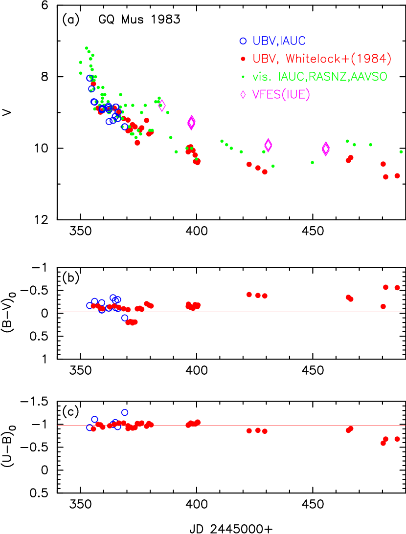
Figure 28 shows the $V$ and visual, $(B-V)_{0}$ , and $(U-B)_{0}$ evolutions of GQ Mus. The $UBV$ data of GQ Mus are taken from Whitelock et al. (1984) and IAU circular Nos. 3766, 3771, and 3853. The $V$ data were observed with the Fine Error Sensor (FES) monitor on board IUE, which are taken from the INES archive data sever⁵⁵5http://sdc.cab.inta-csic.es/ines/index2.html. The visual photometric data are from the Royal Astronomical Society of New Zealand (RASNZ) and by AAVSO (see Hachisu et al., 2008, for more detail). Krautter et al. (1984) estimated the peak brightness to be $m_{V,\rm max}\approx 7.0$ (or $m_{V,\rm max}<7.3$ ). Hachisu et al. (2008) adopted $m_{V,\rm max}\approx 7.2$ after Warner (1995). GQ Mus declined with $t_{2}=15$ and $t_{3}=40$ days (e.g., Warner, 1995). The orbital period of 1.43 hr was detected by Diaz & Steiner (1989).

Paper I and Hachisu & Kato (2015) analyzed the light curve of GQ Mus and determined the reddening as $E(B-V)=0.45\pm 0.05$ from the color-color diagram fit, and the distance modulus in the $V$ band as $(m-M)_{V}=15.7\pm 0.2$ by the time-stretching method (see Paper I and Hachisu & Kato (2015) for details). Here, we adopt $E(B-V)=0.45$ and $(m-M)_{V}=15.7$ for GQ Mus after Paper I and Hachisu & Kato (2015).

Using $E(B-V)=0.45$ and $(m-M)_{V}=15.7$ , we plot the color-magnitude diagram of GQ Mus in Figure 23(d). We superpose the data of T Pyx (green symbols) on the figure. These two tracks almost overlap each other in the middle part of the tracks. We regard GQ Mus as a V1500 Cyg type in the color-magnitude diagram as listed in Table 2, because T Pyx was identified as a V1500 Cyg type. The nova entered the nebular phase no later than UT 1983 March 4, at $m_{V}\approx 10.2$ (Drechsel et al., 1984), which is denoted by an arrow in Figure 23(d), i.e., near the point of $M_{V}=-5.70$ and $(B-V)_{0}=-0.25$ . This starting point of the nebular phase is much ( $\sim 1.7$ mag) above the line of two-headed black arrow.

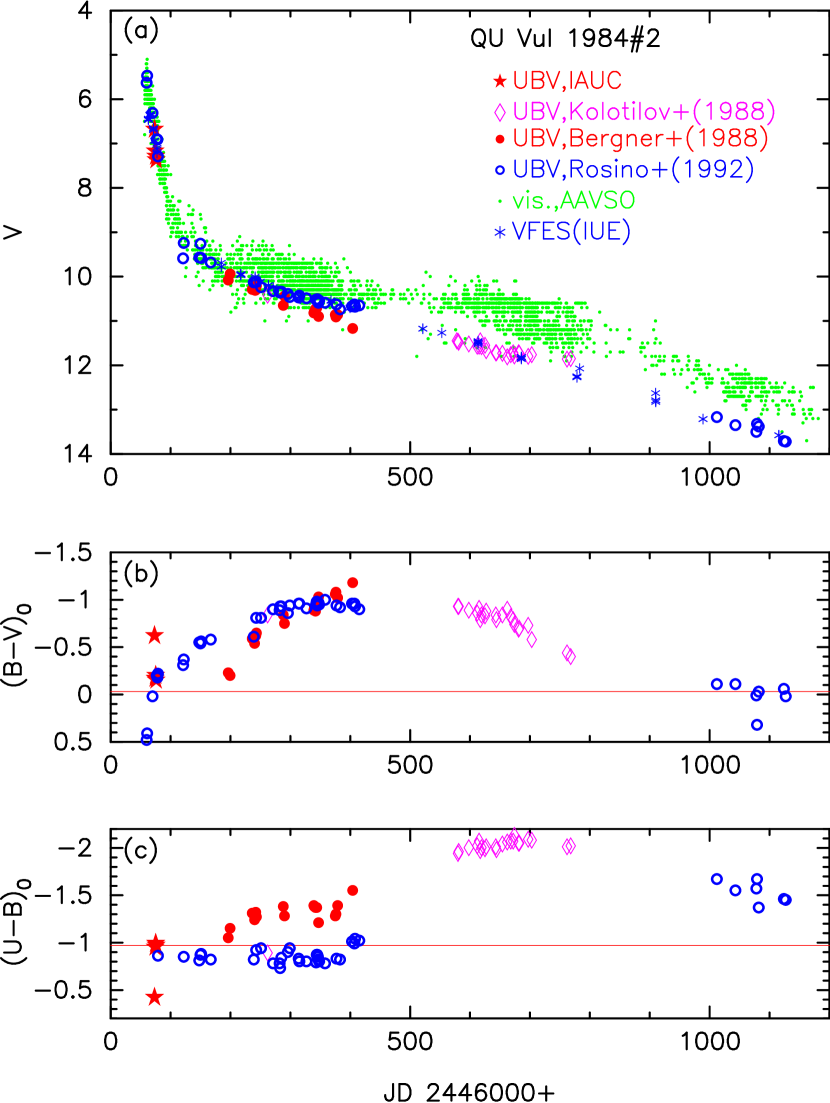
3.9. QU Vul 1984#2

Figure 29 shows the $V$ and visual, $(B-V)_{0}$ , and $(U-B)_{0}$ evolutions of QU Vul. The $UBV$ data of QU Vul are taken from IAU Circular No. 4033, Kolotilov & Shenavrin (1988), Bergner et al. (1988), and Rosino et al. (1992). The visual data are taken from the AAVSO archive. The $B-V$ colors of Rosino et al. (1992) are systematically bluer by 0.1 mag, so we shift them down by 0.1 mag in Figure 29(b). Gehrz et al. (1985) identified QU Vul as a neon nova, and Shafter et al. (1995) detected the orbital period of 2.68 hr.

Paper I and Hachisu & Kato (2016) analyzed the light curve of QU Vul and determined the reddening as $E(B-V)=0.55\pm 0.05$ from the color-color diagram fit and the distance modulus in the $V$ band as $(m-M)_{V}=13.6\pm 0.2$ by the time-stretching method (see Paper I and Hachisu & Kato (2016) for other estimates of reddening and distance). Assuming $E(B-V)=0.55$ , we plot the color-color diagram of QU Vul in Figure 22(c). This figure is the same as Figure 31(c) of Paper I, but we reanalyzed the color data as mentioned above in Figure 29(b). The color-color evolution is consistent with the general tracks of novae. Therefore, we adopt $E(B-V)=0.55$ for QU Vul.

We plot various distance-reddening relations for QU Vul, $(l,b)=(68\fdg 5108,-6\fdg 0263)$ , in Figure 25(c). The thick solid blue line denotes $(m-M)_{V}=13.6$ . The solid magenta line is the relation calculated from the model UV 1455 Å light curve fitting of a $0.96~{}M_{\sun}$ WD model with the chemical composition of Ne nova 3 (Hachisu & Kato, 2016). We also plot the four distance-reddening relations of Marshall et al. (2006). The solid black line is Green et al.’s (2015) relation. These distance-reddening relations cross consistently at/near the point of $d=2.4$ kpc and $E(B-V)=0.55$ . Thus, we adopt a set of $E(B-V)=0.55$ , $d=2.4$ kpc, and $(m-M)_{V}=13.6$ for QU Vul after Hachisu & Kato (2016).

Adopting $E(B-V)=0.55$ and $(m-M)_{V}=13.6$ , we plot the color-magnitude diagram of QU Vul in Figure 30(a). The track of QU Vul roughly overlaps with that of V1974 Cyg, so we regard QU Vul as a V1974 Cyg type in the color-magnitude diagram as listed in Table 2. The nova entered the nebular phase in April 1985 at $m_{V}\approx 9.7$ (Rosino & Iijima, 1987; Rosino et al., 1992) as denoted by an arrow in the figure. We obtain the starting position of the nebular phase at $M_{V}=-4.01$ and $(B-V)_{0}=-0.31$ as denoted by a large open red square. This point is located on the line of the two-headed black arrow. Then the track once made an excursion toward blue up to $(B-V)_{0}\sim-1.0$ followed by the final excursion toward red.

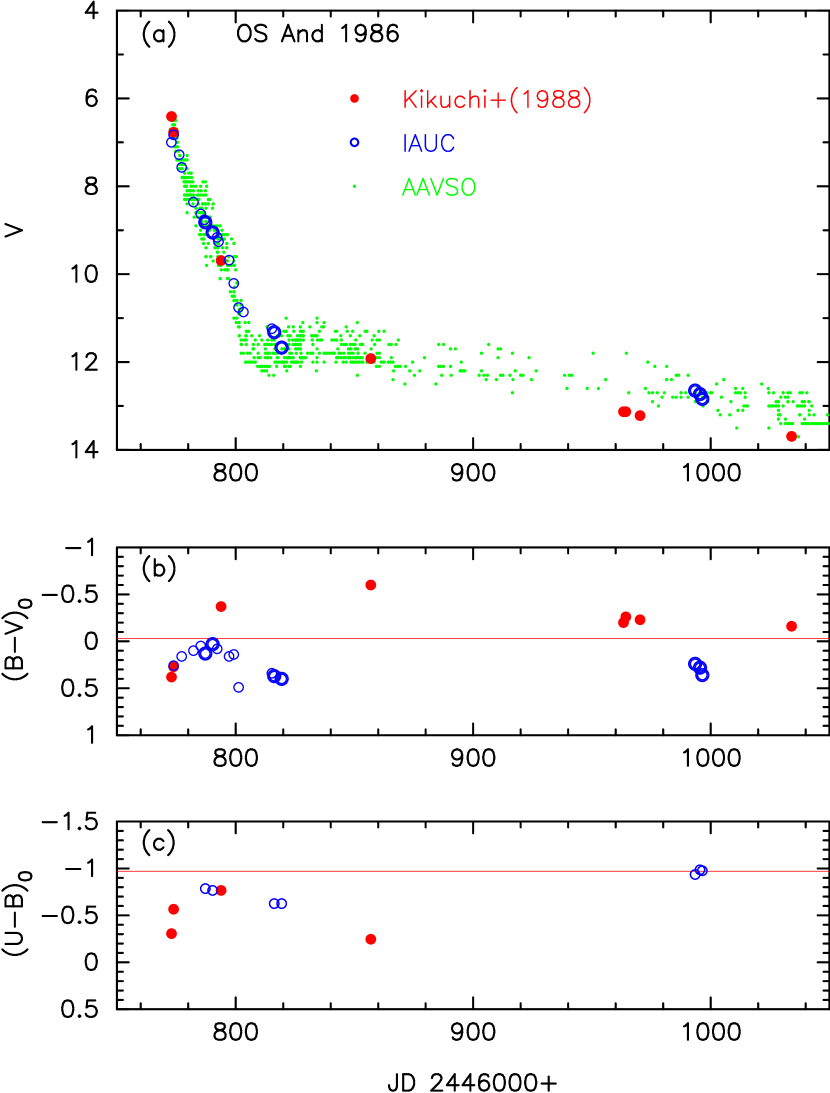
3.10. OS And 1986

Figure 31 shows the visual and $V$ , $(B-V)_{0}$ , and $(U-B)_{0}$ evolutions of OS And on a linear timescale. We have already plotted the same visual and $V$ , $(B-V)_{0}$ , and $(U-B)_{0}$ light curves in Figure 27, but on a logarithmic timescale. The $UBV$ data of OS And are taken from Kikuchi et al. (1988), Ohmori & Kaga (1987), and IAU Circular Nos. 4306, 4342, and 4452.

In Paper I, we determined the reddening as $E(B-V)=0.15\pm 0.05$ from the color-color diagram fit and the distance modulus in the $V$ band as $(m-M)_{V}=14.7\pm 0.2$ by the time-stretching method (see Paper I for other estimates of reddening and distance). We reanalyzed the time-stretching method for V1668 Cyg, V1370 Aql, and OS And in Equation (17) because the distance modulus of V1668 Cyg was revised in Hachisu & Kato (2016). The new distance modulus of OS And is $(m-M)_{V}=14.8\pm 0.2$ . Then the distance is calculated to be $d=7.3$ kpc for $E(B-V)=0.15$ .

We fit our model light curves with the OS And observation, i.e., $V$ and UV 1455 Å light curves. We adopt a $1.05~{}M_{\sun}$ WD model of the CO nova 3 chemical composition (Hachisu & Kato, 2016). This model fits well both the $V$ and UV 1455 Å light curves as shown in Figure 27(a). Here, we plot the three model light curves for V1370 Aql ( $0.95~{}M_{\sun}$ ), V1668 Cyg ( $0.98~{}M_{\sun}$ ), and OS And ( $1.05~{}M_{\sun}$ ) with appropriate time-stretching factors depicted in the figure. The solid blue/red lines are almost the same for V1370 Aql, V1668 Cyg, and OS And, because these model light curves have a universal shape. The $V$ light curve fit gives a relation of $(m-M)_{V}=14.8$ for OS And. We plot the distance-reddening relations in Figure 25(d), i.e., the lines for $(m-M)_{V}=14.8$ (solid blue line), given by Green et al. (2015) (solid black line), and UV 1455 Å model light curve fit (a $1.05~{}M_{\sun}$ WD model with the chemical composition of CO nova 3). These lines cross at/near the point of $d=7.3$ kpc and $E(B-V)=0.15$ . Therefore, we adopt $(m-M)_{V}=14.8$ and $E(B-V)=0.15$ in this paper.

Using $E(B-V)=0.15$ and $(m-M)_{V}=14.8$ , we plot the color-magnitude diagram of OS And in Figure 30(b). The track denoted by open blue squares (data from IAU Circulars) is close to that of FH Ser (solid orange lines), while that denoted by filled red circles (data from Kikuchi et al.) is close to that of V1668 Cyg. We regard OS And as a V1668 Cyg type in the color-magnitude diagram and list it in Table 2. The dust-blackout starts at $M_{V}=-4.59$ and $(B-V)_{0}=+0.14$ , denoted by a large open red square.

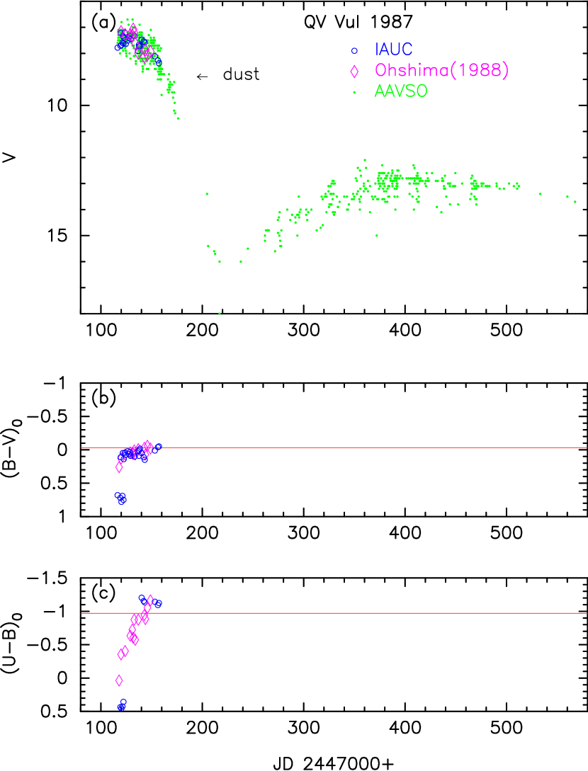
3.11. QV Vul 1987

Figure 32 shows the visual and $V$ , $(B-V)_{0}$ , and $(U-B)_{0}$ evolutions of QV Vul. The $UBV$ data are taken from Ohshima (1988) and IAU Circular Nos. 4493, 4511, and 4524, and the visual data are from the AAVSO archive. We shift the $B-V$ and $U-B$ data of IAU Circulars down by 0.1 and 0.2 mag, respectively, to match these data to those of Ohshima (1988). QV Vul is a dust-blackout type moderately fast nova with $t_{2}=50$ and $t_{3}=53$ days (Downes & Duerbeck, 2000).

In Paper I, we determined the reddening as $E(B-V)=0.60\pm 0.05$ from the color-color diagram fit and the distance modulus in the $V$ band as $(m-M)_{V}=14.0\pm 0.2$ from the time-stretching method (see Paper I for other estimates of reddening and distance). Using $E(B-V)=0.60$ , we plot the color-color track of QV Vul in Figure 22(d). The figure is the same as Figure 32(a) of Paper I, but we added the data of IAU Circulars (open blue circles). The track of QV Vul is consistent with the general track of novae (solid green line), so we adopt $E(B-V)=0.60$ .

We plot various distance-reddening relations for QV Vul, $(l,b)=(53\fdg 8585,+6\fdg 9741)$ , in Figure 33(a), i.e., Marshall et al.’s (2006) four relations, Green et al.’s (2015) relation, $E(B-V)=0.60$ , and $(m-M)_{V}=14.0$ . The various distance-reddening relations cross each other at $E(B-V)=0.60$ and $d=2.7$ kpc. Therefore, we adopt $E(B-V)=0.60$ and $(m-M)_{V}=14.0$ for QV Vul.

Using $(m-M)_{V}=14.0$ and $E(B-V)=0.60$ , we plot the color-magnitude diagram of QV Vul in Figure 30(c). The track is similar to, but slightly bluer than, that of FH Ser. We regard QV Vul as a FH Ser type in the color-magnitude diagram. The dust blackout started at $m_{V}\approx 9.0$ as indicated by an arrow and large open red square at $(B-V)_{0}=-0.03$ and $M_{V}=-5.0$ .

3.12. V443 Sct 1989

Figure 34 shows the visual and $V$ , $(B-V)_{0}$ , and $(U-B)_{0}$ evolutions of V443 Sct. The $UBV$ data are taken from IAU Circular Nos. 4862, 4865, 4868, 4873, and 4902. The photographic magnitudes are taken from IAU Circulars Nos. 4862 and 4868. V443 Sct possibly reached 7.5 mag at maximum (Rosino et al., 1991). The visual magnitudes are from the AAVSO archive. The global shape of the light curve is similar to that of PW Vul (see Figure 52 of Paper I).

In Paper I, we determined the reddening as $E(B-V)=0.40\pm 0.05$ from the color-color diagram fit and the distance modulus in the $V$ band as $(m-M)_{V}=15.5\pm 0.2$ from the time-stretching method (see Paper I for other estimates of reddening and distance). Then, the distance is calculated to be $d=7.1$ kpc for $E(B-V)=0.40$ . We plot various distance-reddening relations in Figure 33(b). The two lines of $E(B-V)=0.40$ and $(m-M)_{V}=15.5$ cross at $d=7.1$ kpc. On the other hand, Green et al.’s (2015) (solid black line) and Marshall et al.’s (2006) four relations cross the line of $(m-M)_{V}=15.5$ at $E(B-V)\approx 0.64$ and $d\approx 5.2$ kpc. Rosino et al. (1991) estimated the reddening as $E(B-V)=0.3$ from the He I line ratios. Anupama et al. (1992) obtained the reddening of $E(B-V)=0.4$ from the Balmer/Paschen line ratios, being consistent with our value. Andreä et al. (1994) estimated the reddening as $E(B-V)=0.30$ from the H and He recombination line ratios. Here, we adopt $E(B-V)=0.40$ and $(m-M)_{V}=15.5$ because the $1\sigma$ error of reddening is rather large for this direction in the Marshall et al.’s relations.

Using $E(B-V)=0.40$ and $(m-M)_{V}=15.5$ , we plot the color-magnitude diagram of V443 Sct in Figure 30(d). The track of V443 Sct is similar to that of PW Vul, which is an LV Vul type, although the number of data points are small. Thus, we regard V443 Sct as an LV Vul type as listed in Table 2. Rosino et al. (1991) reported that the nova had already entered the nebular phase in March 1990 after a period of seasonal invisibility. They also wrote that the nova was approaching the nebular phase in November 1989. Therefore, we specify that the nova entered the nebular phase at $m_{V}\approx 12.0$ , which is denoted by an arrow in Figure 30(d).

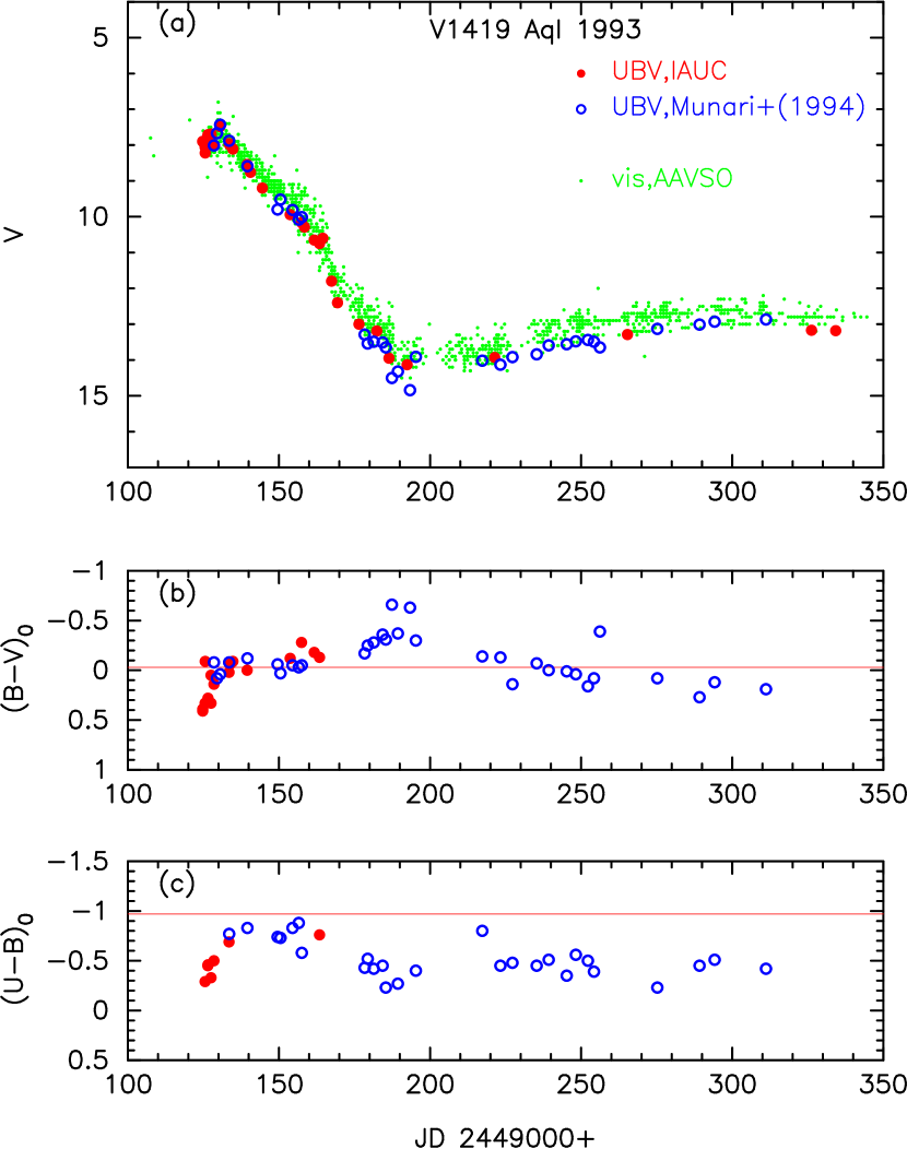
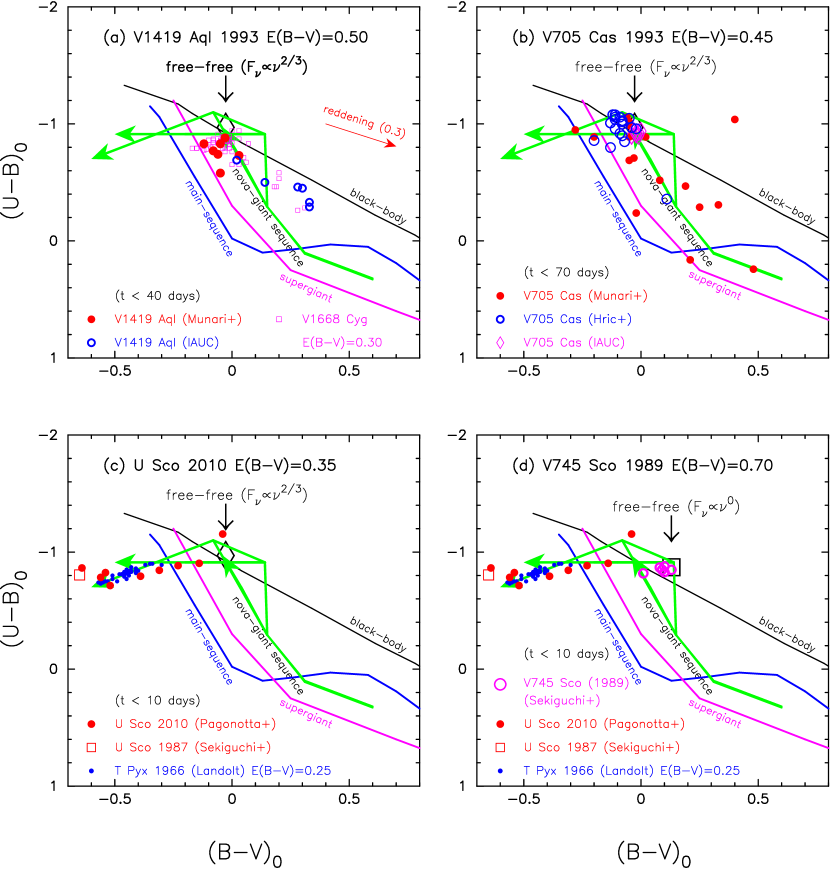
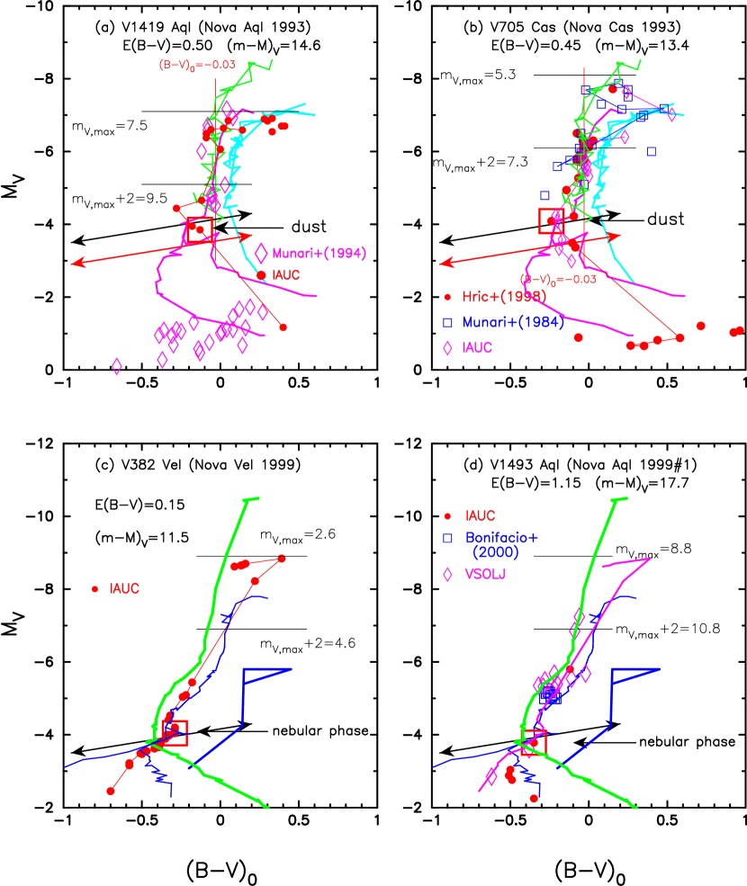
3.13. V1419 Aql 1993

Figure 35 shows the visual and $V$ , $(B-V)_{0}$ , and $(U-B)_{0}$ evolutions of V1419 Aql. The $UBV$ data are taken from Munari et al. (1994a) and IAU Circular Nos. 5794, 5802, 5807, and 5829. The visual magnitudes are from the AAVSO archive. V1419 Aql is a dust-blackout type fast nova with $t_{2}=17$ and $t_{3}=31$ days (Downes & Duerbeck, 2000).

In Paper I, we determined the reddening as $E(B-V)=0.50\pm 0.05$ from the color-color diagram fit and the distance modulus in the $V$ band as $(m-M)_{V}=14.6\pm 0.2$ from the time-stretching method (see Paper I for other estimates of reddening and distance). Then, the distance is calculated to be $d=4.1$ kpc for $(m-M)_{V}=14.6$ and $E(B-V)=0.50$ . We plot various distance-reddening relations in Figure 33(c), which is the same as Figure 36(d) of Paper I, but we added Green et al.’s relation (solid black line). These trends, i.e., $(m-M)_{V}=14.6$ , $E(B-V)=0.50$ , Marshall et al.’s (2006), and Green et al.’s (2015), roughly cross each other at the point of $E(B-V)\approx 0.50$ , $(m-M)_{V}\approx 14.6$ , and $d\approx 4.1$ kpc, the same values as in Paper I.

Adopting $E(B-V)=0.50$ , we plot the color-color diagram of V1419 Aql in Figure 36(a). The figure is the same as Figure 32(c) of Paper I, but we added more data points from Munari et al. (1994a) and the track of V1668 Cyg (small open magenta squares). The color-color evolution of V1419 Aql almost overlaps that of V1668 Cyg. This again confirms that our value of $E(B-V)=0.50\pm 0.05$ is reasonable.

Using $E(B-V)=0.50$ and $(m-M)_{V}=14.6$ , we plot the color-magnitude diagram of V1419 Aql in Figure 37(a). The color-magnitude track of V1419 Aql is also very similar to that of V1668 Cyg except for the maximum brightness. The maximum brightness is close to those of LV Vul and FH Ser. We regard V1419 Aql as a V1668 Cyg type as listed in Table 2. In the color-magnitude diagram, the dust blackout started at $(B-V)_{0}=-0.13$ and $M_{V}=-3.85$ (a large open red square).

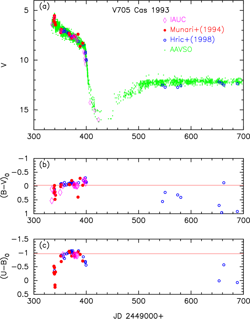
3.14. V705 Cas 1993

Figure 38 shows the visual and $V$ , $(B-V)_{0}$ , and $(U-B)_{0}$ evolutions of V705 Cas. The $UBV$ data are taken from Munari et al. (1994b), Hric et al. (1998), and IAU Circular Nos. 5905, 5912, 5914, 5920, 5928, 5929, 5945, and 5957. The visual data are from the AAVSO archive. V705 Cas is a dust-blackout type nova with $t_{2}=33$ and $t_{3}=61$ days (Hric et al., 1998). The orbital period of 5.47 hr was obtained by Retter & Leibowitz (1995).

Paper I and Hachisu & Kato (2015) determined the reddening as $E(B-V)=0.45\pm 0.05$ and the distance modulus in the $V$ band as $(m-M)_{V}=13.4\pm 0.1$ , both from the model light curve fitting (see Paper I and Hachisu & Kato (2015) for other estimates of reddening and distance). We plot three distance-reddening relations in Figure 33(d). Hachisu & Kato (2015) fitted their model light curves of a $0.78~{}M_{\sun}$ WD of CO nova 4 chemical composition with the V705 Cas observation. The $V$ light curve fit gives $(m-M)_{V}=13.4$ , and the UV 1455 Å light curve fit also yields that of the solid magenta line in Figure 33(d). The solid black line is the distance-reddening relation given by Green et al. (2015). These trends roughly cross each other at the point of $d\approx 2.5$ kpc, $E(B-V)\approx 0.45$ , and $(m-M)_{V}\approx 13.4$ . Therefore, we adopt $E(B-V)=0.45$ and $(m-M)_{V}=13.4$ , the same as those in Paper I and Hachisu & Kato (2015).

Using $E(B-V)=0.45$ , we plot the color-color diagram of V705 Cas in Figure 36(b). Because the dust-blackout started about 60 days after discovery, we plot only the data for $t<70$ days. This figure is the same as Figure 32(d) of Paper I, but we reanalyzed the color data. The color-color evolution is consistent with the general track of novae (solid green lines). This again confirms our value of $E(B-V)=0.45\pm 0.05$ .

Using $E(B-V)=0.45$ and $(m-M)_{V}=13.4$ , we plot the color-magnitude diagram of V705 Cas in Figure 37(b). V705 Cas moves along a flat circle anti-clockwise in the very early phase near maximum. After that, it follows the track of FH Ser and then goes along the track of V1668 Cyg. We regard V705 Cas as a V1668 Cyg type. The nova entered a dust blackout phase at the position of $(B-V)_{0}=-0.20$ and $M_{V}=-4.09$ .

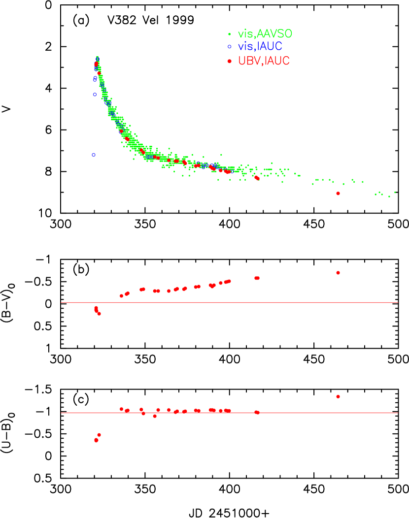
3.15. V382 Vel 1999

Figure 39 shows the visual and $V$ , $(B-V)_{0}$ , and $(U-B)_{0}$ evolutions of V382 Vel. The $UBV$ data are taken from IAU Circular Nos. 7176, 7179, 7196, 7209, 7216, 7226, 7232, and 7277. The visual magnitudes are taken from IAU Circulars and AAVSO archive. V382 Vel was identified as a very fast neon nova (Woodward et al., 1999). The orbital period of 3.5 hr was detected by Balman et al. (2006).

In Paper I and Hachisu & Kato (2016), we determined the reddening as $E(B-V)=0.15\pm 0.05$ and the distance modulus in the $V$ band as $(m-M)_{V}=11.5\pm 0.1$ , both from the model light curve fitting (see Paper I and Hachisu & Kato (2016) for other estimates of reddening and distance). Using $E(B-V)=0.15$ and $(m-M)_{V}=11.5$ , we plot the color-magnitude diagram of V382 Vel in Figure 37(c). The color-magnitude diagram of V382 Vel almost coincides with the track of V1974 Cyg. Therefore, we regard V382 Vel as a V1974 Cyg type in the color-magnitude diagram. The distance is calculated to be $d=1.6$ kpc for $E(B-V)=0.15$ and $(m-M)_{V}=11.5$ .

della Valle et al. (2002) reported that the nebular phase started at least by the end of 1999 June, i.e., $\sim 40$ days after the optical maximum. We plot this phase ( $M_{V}=m_{V}-(m-M)_{V}\approx 7.4-11.5=-4.1$ ) by an arrow in Figure 37(c). Then we can specify the position of a cusp point to $(B-V)_{0}=-0.29$ and $M_{V}=-4.04$ as denoted by a large open red square.

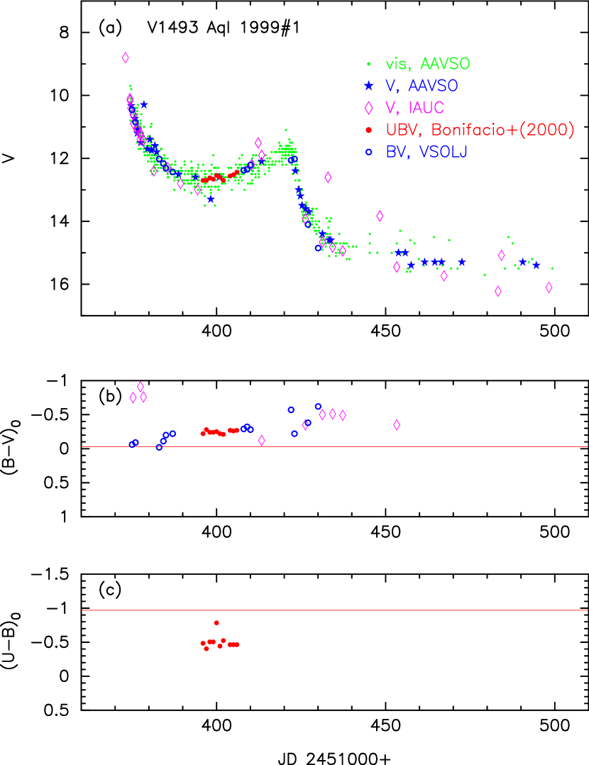
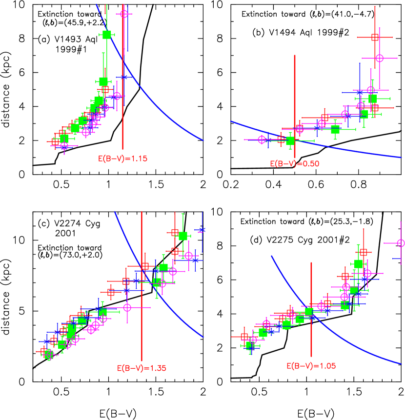
3.16. V1493 Aql 1999#1

This nova is not studied in Paper I. Figure 40 shows the visual and $V$ , $(B-V)_{0}$ , and $(U-B)_{0}$ evolutions of V1493 Aql. The $UBV$ data are taken from Bonifacio et al. (2000). The $BV$ data are from the VSOLJ archive and IAU Circular Nos. 7228, 7254, 7273, and 7313. The peak could be missed, so we may assume $m_{V,\rm max}=8.8$ for this nova. It quickly decayed with $t_{2}=3$ days (Bonifacio et al., 2000) or with $t_{2}=7$ and $t_{3}=24$ days (Venturini et al., 2004). Therefore, V1493 Aql belongs to the class of very fast novae. The light curve of V1493 Aql has a prominent secondary maximum about 50 days after the optical maximum (e.g., Bonifacio et al., 2000; Hachisu & Kato, 2009). Dobrotka et al. (2006) obtained an orbital period of 3.74 hr. The observational period of the $U$ band is too short to derive $E(B-V)$ from the general course of nova tracks (Figure 40(c)). Therefore, we could not estimate the extinction from the color-color diagram of V1493 Aql. We show the $V$ light curve, $(B-V)_{0}$ , and $(U-B)_{0}$ color evolutions in a logarithmic timescale in Figure 41 together with the three fast novae, V2275 Cyg, V382 Vel, and V1500 Cyg, which have similar decline rates.

The reddening for V1493 Aql was estimated as $E(B-V)=0.33\pm 0.1$ (Bonifacio et al., 2000) from the intrinsic $B-V$ color at $t_{2}$ , to be $E(B-V)=1.5$ (Arkhipova et al., 2002) from the Balmer decrement (mostly first Balmer lines), and to be $E(B-V)=0.57\pm 0.14$ (Venturini et al., 2004) from the dust reddening curve of Draine (1989). These three values are very different from each other. Therefore, we made a new estimate assuming that the intrinsic $B-V$ color of V1493 Aql is similar to those of V1500 Cyg, V382 Vel, and V2275 Cyg as shown in Figure 41(b). Then we obtain the color excess of $E(B-V)=1.15\pm 0.05$ .

Using the time-stretching method as plotted in Figure 41(a), we obtain the apparent distance modulus in $V$ as follows:

$\displaystyle(m-M)_{V,\rm V1493~{}Aql}$	$\displaystyle=$	$\displaystyle 17.7$	(18)
	$\displaystyle=$	$\displaystyle(m-M+\Delta V)_{V,\rm V1500~{}Cyg}-2.5\log 1.0/1.0$	(19)
	$\displaystyle=$	$\displaystyle 12.3+(+4.0+1.4)+0.0=17.7$	(20)
	$\displaystyle=$	$\displaystyle(m-M+\Delta V)_{V,\rm V382~{}Vel}-2.5\log 0.85/1.0$	(21)
	$\displaystyle\approx$	$\displaystyle 11.5+(+4.6+1.4)+0.18=17.68$	(22)
	$\displaystyle=$	$\displaystyle(m-M+\Delta V)_{V,\rm V2275~{}Cyg}-2.5\log 1.0/1.0$	(23)
	$\displaystyle=$	$\displaystyle 16.3+(+0.0+1.4)+0.0=17.7,$	(24)

where we use $(m-M)_{V,\rm V1500~{}Cyg}=12.3$ from Section 2.5, $(m-M)_{V,\rm V382~{}Vel}=11.5$ from Section 3.15, and $(m-M)_{V,\rm V2275~{}Cyg}=16.3$ from Section 3.19. Therefore, we adopt $(m-M)_{V}=17.7$ for V1493 Aql.

Figure 42(a) shows various distance-reddening relations for V1493 Aql, $(l,b)=(45\fdg 9080,+2\fdg 1551)$ . Here we plot four nearby directions calculated by Marshall et al. (2006), i.e., $(l,b)=(45\fdg 75,2\fdg 25)$ denoted by open red squares, $(46\fdg 00,2\fdg 25)$ by filled green squares, $(45\fdg 75,2\fdg 00)$ by blue asterisks, and $(46\fdg 00,2\fdg 00)$ by open magenta circles. We also plot the distance-reddening relation (solid black line) given by Green et al. (2015). The two lines of $E(B-V)=1.15$ and $(m-M)_{V}=17.7$ cross at the point $d=6.7$ kpc and $E(B-V)=1.15$ . This position is consistent with the distance-reddening relation of Marshall et al. (2006) but deviates slightly from that of Green et al. (2015).

Using $E(B-V)=1.15$ and $(m-M)_{V}=17.7$ , we plot the color-magnitude diagram of V1493 Aql in Figure 37(d). The track of V1493 Aql is located near the tracks of V382 Vel and V1974 Cyg. We regard V1493 Aql as a V1974 Cyg type in the color-magnitude diagram. The nova was clearly in the nebular phase on UT 1999 September 16 at $m_{V}\sim 15$ , i.e., about 65 days after the discovery (Arkhipova et al., 2002), while the nebular lines began to grow on UT 1999 August 4 ( $m_{V}\sim 13$ ). We could specify a possible start ( $m_{V}\sim 14$ ) of the nebular phase at the point $(B-V)_{0}=-0.35$ and $M_{V}=-3.78$ , which is denoted by a large open square in Figure 37(d).

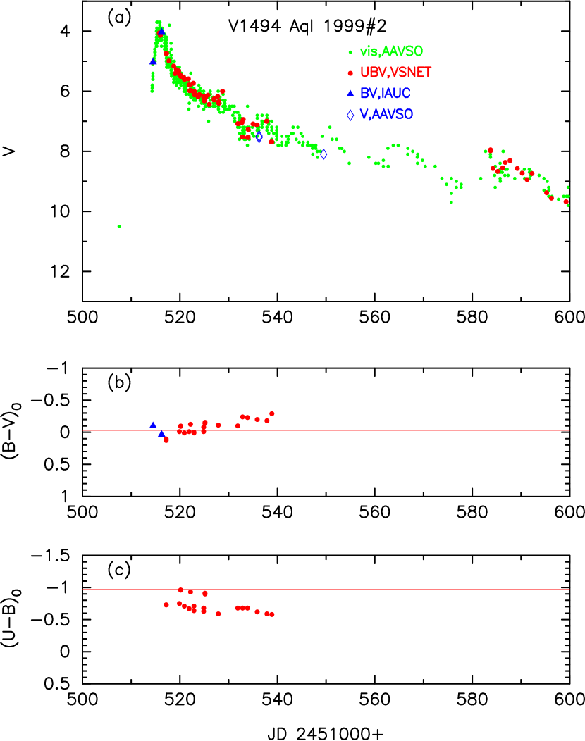
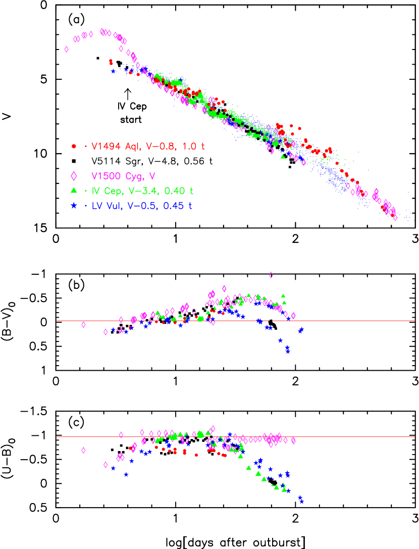
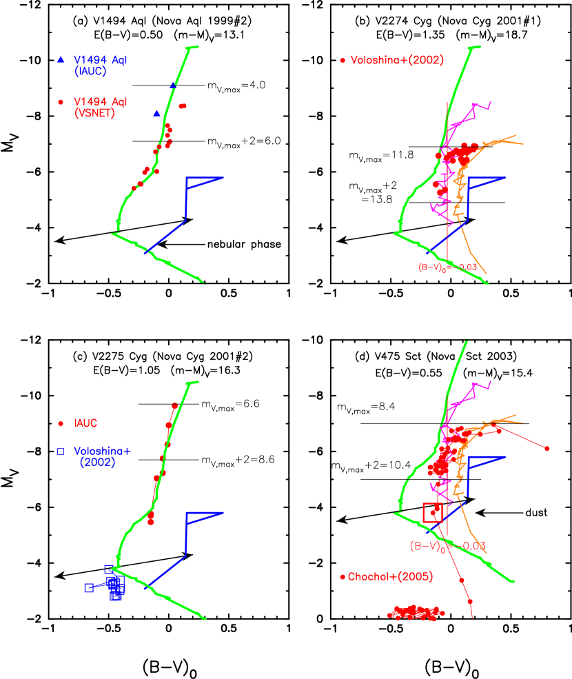
3.17. V1494 Aql 1999#2

This nova is not studied in Paper I. Figure 43 shows the visual and $V$ , $(B-V)_{0}$ , and $(U-B)_{0}$ evolutions of V1494 Aql. The $UBV$ data are taken from the VSNET archive. The $BV$ data are from IAU Circulars Nos. 7324 and 7327. The visual data are from the AAVSO archive. V1494 Aql reached its maximum of $m_{V,\rm max}=4.0$ on UT 1999 December 3.4. V1494 Aql is a very fast nova with $t_{2}=6.6\pm 0.5$ and $t_{3}=16\pm 0.5$ days (Kiss & Thomson, 2000). The orbital period of 3.23 hr was detected by Retter et al. (2000) and Barsukova & Goranskii (2003).

The reddening for V1494 Aql was estimated by Iijima & Esenoglu (2003) to be $E(B-V)=0.6\pm 0.1$ from the interstellar Na I D1 and D2 lines. We could not estimate the extinction from the color-color diagram of V1494 Aql because there is a large scatter in the $U-B$ data. Instead, we use Figure 44(b) and obtain $E(B-V)=0.50\pm 0.05$ assuming that the intrinsic $(B-V)_{0}$ color evolution of V1494 Aql is similar to those of the other color evolutions. This value is consistent with that obtained by Iijima & Esenoglu (2003).

Using the time-stretching method (see Figure 44(a)), we obtain

$\displaystyle(m-M)_{V,\rm V1494~{}Aql}$	$\displaystyle=$	$\displaystyle 13.1$	(25)
	$\displaystyle=$	$\displaystyle(m-M+\Delta V)_{V,\rm V1500~{}Cyg}-2.5\log 1.0/1.0$	(26)
	$\displaystyle=$	$\displaystyle 12.3+(-0.0+0.8)+0.0\approx 13.10$	(27)
	$\displaystyle=$	$\displaystyle(m-M+\Delta V)_{V,\rm IV~{}Cep}-2.5\log 0.40/1.0$	(28)
	$\displaystyle\approx$	$\displaystyle 14.7+(-3.4+0.8)+0.99\approx 13.09$	(29)
	$\displaystyle=$	$\displaystyle(m-M+\Delta V)_{V,\rm LV~{}Vul}-2.5\log 0.45/1.0$	(30)
	$\displaystyle\approx$	$\displaystyle 11.9+(-0.5+0.8)+0.87\approx 13.07$	(31)
	$\displaystyle=$	$\displaystyle(m-M+\Delta V)_{V,\rm V5114~{}Sgr}-2.5\log 0.56/1.0$	(32)
	$\displaystyle\approx$	$\displaystyle 16.5+(-4.8+0.8)+0.63\approx 13.13,$	(33)

where we use $(m-M)_{V,\rm V1500~{}Cyg}=12.3$ from Section 2.5, $(m-M)_{V,\rm IV~{}Cep}=14.7$ from Section 3.5, $(m-M)_{V,\rm LV~{}Vul}=11.9$ from Section 2.2, and $(m-M)_{V,\rm V5114~{}Sgr}=16.5$ from Section 3.21. Because these values are consistent with each other, we adopt $(m-M)_{V}=13.1$ for V1494 Aql.

Figure 42(b) shows various distance-reddening relations for V1494 Aql, $(l,b)=(40\fdg 9735,-4\fdg 7422)$ . Here we plot the distance-reddening relations calculated by Marshall et al. (2006), i.e., for nearby directions, $(l,b)=(40\fdg 75,-4\fdg 50)$ denoted by open red squares, $(41\fdg 00,-4\fdg 50)$ by filled green squares, $(40\fdg 75,-4\fdg 75)$ by blue asterisks, and $(41\fdg 00,-4\fdg 75)$ by open magenta circles. The closest one is that denoted by open magenta circles. We also plot the distance-reddening relation (solid black line) given by Green et al. (2015). The two lines of $E(B-V)=0.50$ and $(m-M)_{V}=13.1$ cross at the distance of $d=2.0$ kpc and $E(B-V)=0.50$ . This cross point is consistent with Marshall et al.’s relation, but slightly different from that of Green et al.’s.

Using $E(B-V)=0.50$ and $(m-M)_{V}=13.1$ , we plot the color-magnitude diagram of V1494 Aql in Figure 45(a). The track is very similar to that of V1500 Cyg in the middle part of the whole track. We regard V1494 Aql as a V1500 Cyg type in the color-magnitude diagram. The nebular phase started at least before the middle of 2000 April, i.e., around $m_{V}\sim 10$ (Iijima & Esenoglu, 2003). We plot this phase by an arrow in Figure 45(a). However, there are no $B-V$ data around the starting point of the nebular phase.

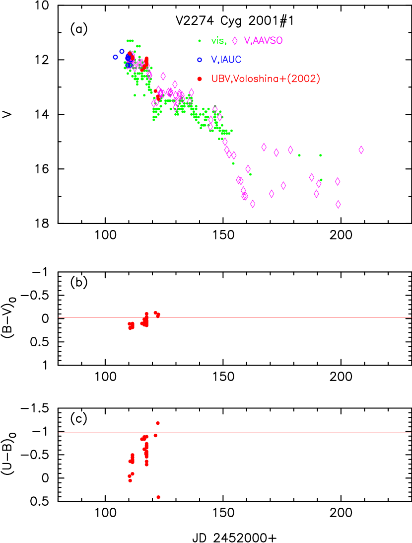
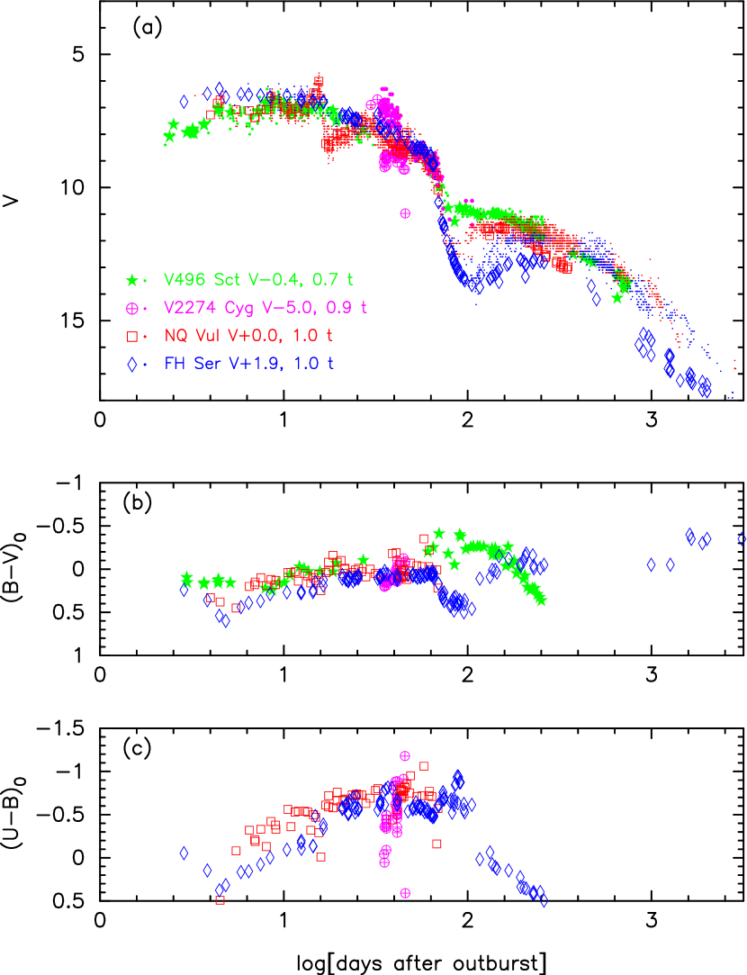
3.18. V2274 Cyg 2001#1

Figure 46 shows the visual and $V$ , $(B-V)_{0}$ , and $(U-B)_{0}$ evolutions of V2274 Cyg. The $UBV$ data are taken from Voloshina & Metlova (2002a), $V$ data are from the AAVSO archive and IAU Circular Nos. 7666 and 7668.

In Paper I, we determined the reddening as $E(B-V)=1.35\pm 0.10$ from the color-color diagram fit and the distance modulus in the $V$ band as $(m-M)_{V}=18.7\pm 0.2$ from the time-stretching method (see Paper I for other estimates of reddening and distance).

The light curve of V2274 Cyg is similar to those of FH Ser and NQ Vul and these three nova light curves have similar decline trends just before the dust blackout as shown in Figure 47(a). From the time-stretching method, we obtain the apparent distance modulus of V2274 Cyg:

$\displaystyle(m-M)_{V,\rm V2274~{}Cyg}$	$\displaystyle=$	$\displaystyle(m-M+\Delta V)_{V,\rm FH~{}Ser}-2.5\log 0.9$	(34)
	$\displaystyle=$	$\displaystyle 11.7+(+1.9+5.0)+0.11=18.71$	(35)
	$\displaystyle=$	$\displaystyle(m-M+\Delta V)_{V,\rm NQ~{}Vul}-2.5\log 0.9$	(36)
	$\displaystyle=$	$\displaystyle 13.6+(+0.0+5.0)+0.11=18.71,$	(37)

where we use $(m-M)_{V,\rm FH~{}Ser}=11.7$ from Section 2.3 and $(m-M)_{V,\rm NQ~{}Vul}=13.6$ from Section 3.6. We adopt this distance modulus of $(m-M)_{V,\rm V2274~{}Cyg}=18.7$ . The distance is estimated as $d=8.0$ kpc for $E(B-V)=1.35$ .

Figure 42(c) shows various distance-reddening relations for V2274 Cyg, $(l,b)=(73\fdg 0415,+1\fdg 9910)$ . This figure is the same as Figure 37(b) of Paper I, but we added the distance-reddening relations given by Green et al. (2015). The two lines of $E(B-V)=1.35$ and $(m-M)_{V}=18.7$ cross at the distance of $d=8.0$ kpc, which is consistent with Marshall et al.’s and Green et al.’s relations.

Using $E(B-V)=1.35$ and $(m-M)_{V}=18.7$ , we plot the color-magnitude diagram of V2274 Cyg in Figure 45(b). The track of V2274 Cyg is close to those of FH Ser and V1668 Cyg. We regard V2274 Cyg as a V1668 Cyg type in the color-magnitude diagram, because V2274 Cyg goes down along the track of V1668 Cyg.

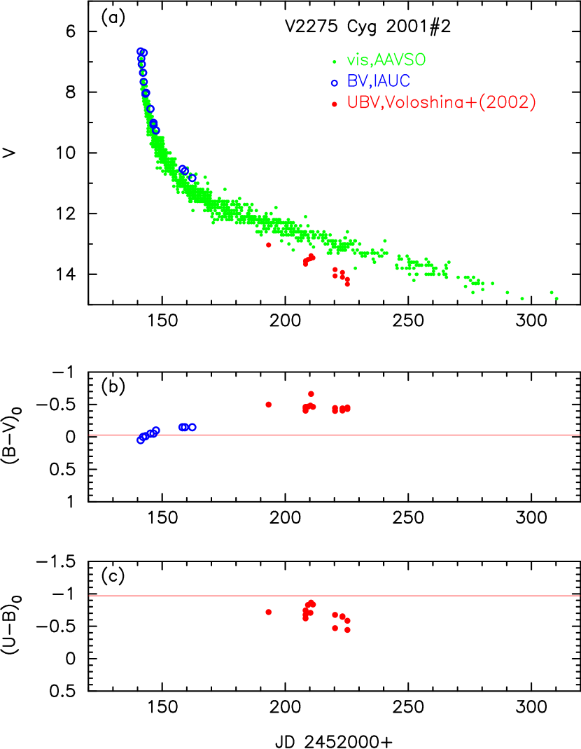
3.19. V2275 Cyg 2001#2

This nova is not studied in Paper I. Figure 48 shows the visual and $V$ , $(B-V)_{0}$ , and $(U-B)_{0}$ evolutions of V2275 Cyg. The $V$ maximum is $m_{V,\rm max}=6.6$ (e.g., Sostero et al., 2001). Then it gradually declined with $t_{2}=2.9$ and $t_{3}=7$ days (Kiss et al., 2002). The $V$ light curve of V2275 Cyg and its decay rate are very similar to those of V1500 Cyg. We could not estimate the extinction from the color-color diagram of V2275 Cyg because no $UBV$ data in the early phase are available. $UBV$ data were secured only in the nebular phase (Voloshina et al., 2002b). Balman (2005) suggested an orbital period of 7.55 hr from photometric orbital variations.

The $V$ light curve shape and global timescale of V2275 Cyg is very similar to that of V1500 Cyg. Assuming that these two novae have the same brightness in the free-free emission phase, i.e., applying the time-stretching method to Figure 41(a), we obtain

	$\displaystyle(m-M)_{V,\rm V2275~{}Cyg}$	$\displaystyle=$	$\displaystyle(m-M+\Delta V)_{V,\rm V1500~{}Cyg}$		(38)
		$\displaystyle=$	$\displaystyle 12.3+4.0=16.3,$		(39)

where we use $(m-M)_{V,\rm V1500~{}Cyg}=12.3$ from Section 2.5. We adopt this value of $(m-M)_{V,\rm V2275~{}Cyg}=16.3$ in the present paper.

Kiss et al. (2002) estimated the absolute magnitude at maximum to be $M_{V,\rm max}=-9.7$ from the MMRD relations and other empirical relations together with $t_{2}=2.9\pm 0.5$ days and $t_{3}=7\pm 1$ days. Then we calculate the apparent distance modulus of $(m-M)_{V}=6.6-(-9.7)=16.3$ , being coincident with our value of $(m-M)_{V}=16.3$ .

Kiss et al. (2002) also discussed that V2275 Cyg closely resembles, in some respects, the well-studied very fast nova V1500 Cyg. Assuming that the intrinsic $B-V$ color is almost the same for V2275 Cyg and V1500 Cyg, we determine the reddening to be $E(B-V)=1.05\pm 0.05$ by overlapping them as shown in Figure 41(b). This estimate is also consistent with the Kiss et al. value of $E(B-V)=1.0\pm 0.1$ , obtained with a few interstellar absorption laws. We adopt $E(B-V)=1.05\pm 0.05$ in this paper.

Figure 42(d) shows various distance-reddening relations for V2275 Cyg, $(l,b)=(89\fdg 3170,+1\fdg 3905)$ . Here we plot distance-reddening relations calculated by Marshall et al. (2006), i.e., four nearby directions, $(l,b)=(89\fdg 25,+1\fdg 25)$ denoted by open red squares, $(89\fdg 50,+1\fdg 25)$ by filled green squares, $(89\fdg 25,+1\fdg 50)$ by blue asterisks, and $(89\fdg 50,+1\fdg 50)$ by open magenta circles. The closest one is that denoted by blue asterisks. We also plot Green et al.’s (2015) distance-reddening relation in the same figure. These four trends, Marshall et al.’s (blue asterisks), Green et al.’s (solid black line), $(m-M)_{V}=16.3$ (solid blue line), and $E(B-V)=1.05$ (vertical solid black line), cross at the point $E(B-V)\approx 1.05$ and $d\approx 4.1$ kpc. Thus, we confirm that our estimates of $E(B-V)=1.05$ and $(m-M)_{V}=16.3$ are reasonable.

Using $E(B-V)=1.05$ and $(m-M)_{V}=16.3$ , we plot the color-magnitude diagram of V2275 Cyg in Figure 45(c). The two nova tracks of V2275 Cyg and V1500 Cyg overlap each other in the color-magnitude diagram. Therefore, we regard V2275 Cyg as a V1500 Cyg type in the color-magnitude diagram.

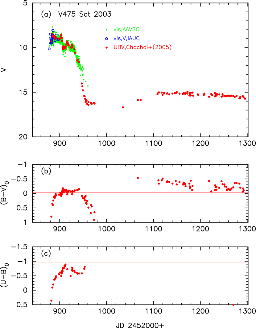
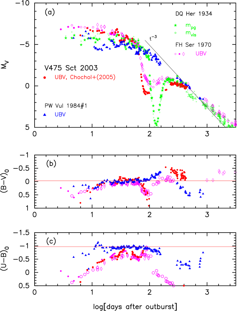
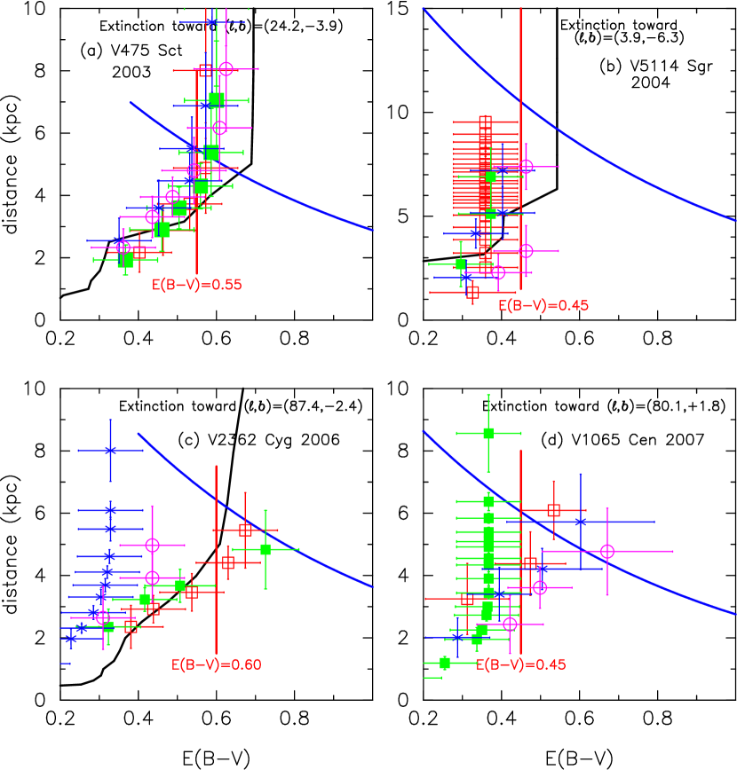
3.20. V475 Sct 2003

Figure 49 shows the visual and $V$ , $(B-V)_{0}$ , and $(U-B)_{0}$ evolutions of V475 Sct. The $UBV$ data are taken from Chochol et al. (2005), $V$ and visual data are from IAU Circular Nos. 8190 and 8200, and the AAVSO archive.

In Paper I, we determined the reddening $E(B-V)=0.55\pm 0.10$ from the color-color diagram fit and the distance modulus in the $V$ band as $(m-M)_{V}=15.6\pm 0.2$ by assuming that the absolute magnitude of the light curve is the same for FH Ser and V475 Sct (see Paper I for other estimates of reddening and distance). To confirm this similarity, we plot the light curves of V475 Sct, FH Ser, PW Vul, and DQ Her in Figure 50, but we adopt $(m-M)_{V}=15.4$ rather than the $(m-M)_{V}=15.6$ of Paper I for V475 Sct. If we use $(m-M)_{V}=15.4$ , the absolute brightness of V475 Sct and FH Ser almost overlap.

Figure 51(a) shows various distance-reddening relations for V475 Sct, $(l,b)=(24\fdg 2015,-3\fdg 9466)$ , i.e., the relations given by Marshall et al. (2006) and Green et al. (2015). Our new estimates of $(m-M)_{V}=15.4$ and $E(B-V)=0.55$ cross at $d=5.5$ kpc, which is roughly consistent with trend of Marshall et al., but deviates from that of Green et al. Thus, we adopt $E(B-V)=0.55$ and $(m-M)_{V}=15.4$ in this paper.

The color-magnitude diagram of V475 Sct is plotted in Figure 45(d). The track is similar to that of FH Ser in the early phase, but to that of V1668 Cyg in the later phase. We regard V475 Sct as a V1668 Cyg type in the color-magnitude diagram. We specify a starting point of dust blackout, that is, $(B-V)_{0}=-0.15$ and $M_{V}=-3.80$ denoted by a large open red square in Figure 45(d).

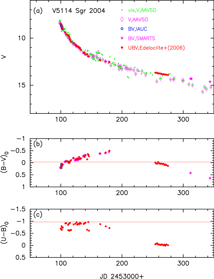
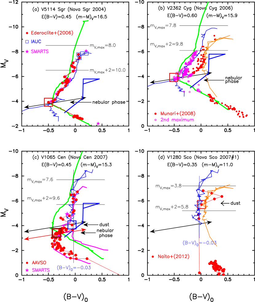
3.21. V5114 Sgr 2004

Figure 52 shows the visual and $V$ , $(B-V)_{0}$ , and $(U-B)_{0}$ evolutions of V5114 Sgr. The $UBV$ data are taken from Ederoclite et al. (2006), $BV$ data from the SMARTS archive and IAU Circular Nos. 8306 and 8310, and visual and $V$ data from the AAVSO archive.

In Paper I, we determined the reddening as $E(B-V)=0.45\pm 0.05$ from the color-color diagram fit and the distance modulus in the $V$ band as $(m-M)_{V}=16.5\pm 0.2$ from the time-stretching method (see Paper I for other estimates of reddening and distance). Then, the distance is calculated to be $d=10.5$ kpc. Figure 51(b) shows various distance-reddening relations for V5114 Sgr, $(l,b)=(3\fdg 9429,-6\fdg 3121)$ . This figure is the same as Figure 37(d) of Paper I, but we added the distance-reddening relation given by Green et al. (2015). The three trends, Marshall et al.’s trend, $(m-M)_{V}=16.5$ , and $E(B-V)=0.45$ , consistently cross at $d\sim 10.5$ kpc and $E(B-V)\sim 0.45$ , although Green et al.’s relation deviates from this cross point. Thus, we adopt the same values of $(m-M)_{V}=16.5$ and $E(B-V)=0.45$ as those in Paper I.

Using $E(B-V)=0.45$ and $(m-M)_{V}=16.5$ , we plot the color-magnitude diagram of V5114 Sgr in Figure 53(a). The track is close to those of V1500 Cyg (thick solid green line) and V1974 Cyg (thin solid blue line). This matching also supports our values of $E(B-V)=0.45$ and $(m-M)_{V}=16.5$ . We regard V5114 Sgr as a V1974 Cyg type in the color-magnitude diagram. We also specify a turning point of $(B-V)_{0}=-0.50$ and $M_{V}=-3.92$ , which is denoted by a large open red square in Figure 53(a). The nebular phase started around 57 days after optical maximum, when the [O III] lines became stronger than the permitted lines (see Figure 3 of Ederoclite et al., 2006).

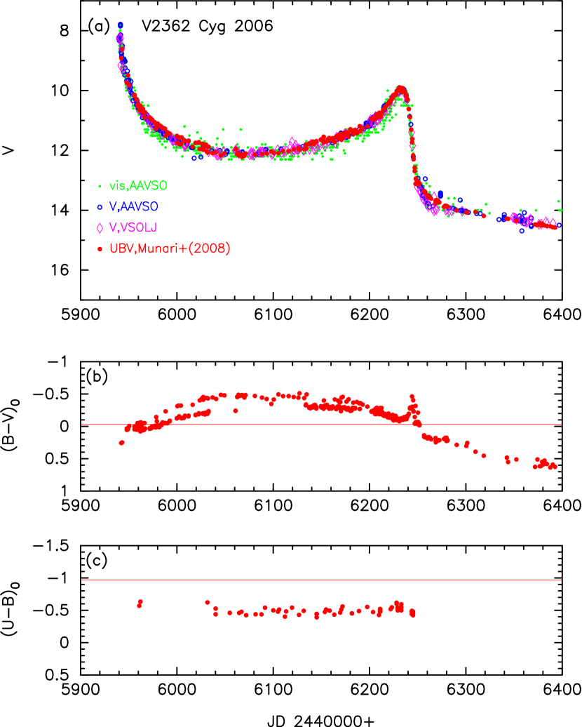
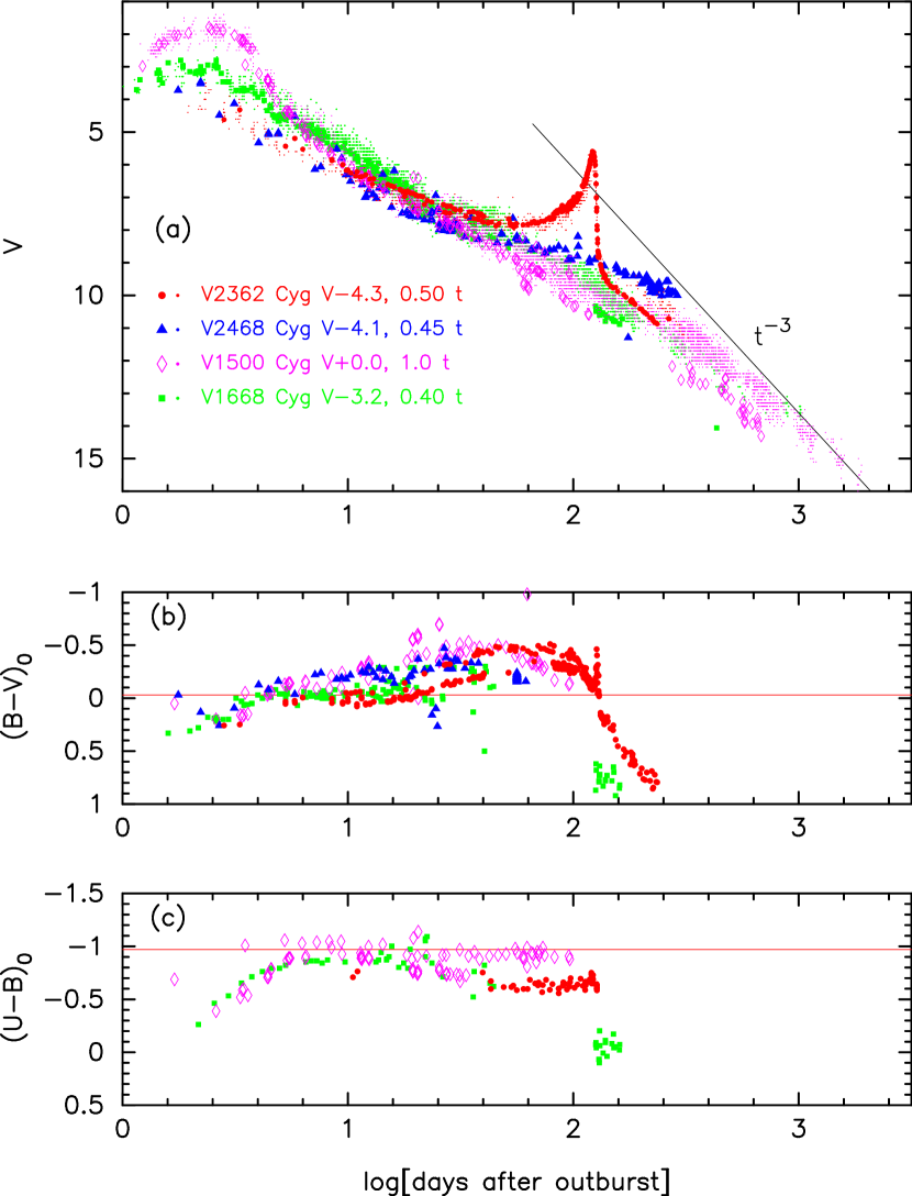
3.22. V2362 Cyg 2006

This nova is not studied in Paper I. Figure 54 shows the visual and $V$ , $(B-V)_{0}$ , and $(U-B)_{0}$ evolutions of V2362 Cyg. The $UBV$ data are taken from Munari et al. (2008b), $V$ and visual from the AAVSO and VSOLJ archives. V2362 Cyg reached $m_{V,\rm max}=7.8$ at optical maximum and then declined with $t_{2}=9.0\pm 0.5$ and $t_{3}=21.0\pm 0.5$ days (Kimeswenger et al., 2008). For the first 60 days, the decline down to 12th magnitude is smooth and resembles a power-law decline. Then it rose up again to 10th magnitude (secondary maximum) about 240 days after the discovery, and suddenly dropped to 13th magnitude in $\sim 20$ days, followed by the formation of an optically thin dust shell (Arai et al., 2010), and again slowly declined resembling a power law before the secondary maximum (e.g., Kimeswenger et al., 2008). An orbital period of 1.58 hr was suggested by Balman et al. (2009).

The reddening of V2362 Cyg was obtained to be $E(B-V)=(B-V)_{t2}-(B-V)_{0,t2}=0.58\pm 0.03-(-0.02\pm 0.12)=0.6\pm 0.1$ (Kimeswenger et al., 2008), $E(B-V)=0.58\pm 0.04$ (Lynch et al., 2008a) from Lyman $\beta$ fluoresced O I lines, $E(B-V)=0.56$ from the equivalent width of interstellar lines Na I D1 and D2, and $E(B-V)=(B-V)_{t2}-(B-V)_{0,t2}=0.54-(-0.02)=0.56$ (Munari et al., 2008b). The NASA/IPAC galactic dust absorption map gives $E(B-V)=0.65\pm 0.03$ in the direction toward V2362 Cyg, $(l,b)=(87\fdg 3724,-2\fdg 3574)$ . Because there are not enough $U$ data in the first decline phase as shown in Figure 54(c), we cannot accurately determine the color excess from the general track fitting in the color-color diagram. Instead, we obtained $E(B-V)=0.60\pm 0.05$ by averaging the above four estimates. Assuming that $E(B-V)=0.60$ , we plot the $(B-V)_{0}$ and $(U-B)_{0}$ color evolutions of V2362 Cyg in Figure 54(b) and 54(c), respectively, and in Figure 55(b) and 55(c) together with V1500 Cyg, V1668 Cyg, and V2468 Cyg. The color evolution is similar to each other. Therefore, we adopt $E(B-V)=0.60\pm 0.05$ in this paper.

Using the time-stretching method (Figure 55(a)), we obtain the apparent distance modulus of V2362 Cyg

$\displaystyle(m-M)_{V,\rm V2362~{}Cyg}$	$\displaystyle=$	$\displaystyle 15.9$	(40)
	$\displaystyle=$	$\displaystyle(m-M+\Delta V)_{V,\rm V2468~{}Cyg}-2.5\log 0.45/0.50$	(41)
	$\displaystyle\approx$	$\displaystyle 15.6+(-4.1+4.3)+0.11=15.91$	(42)
	$\displaystyle=$	$\displaystyle(m-M+\Delta V)_{V,\rm V1500~{}Cyg}-2.5\log 1.0/0.50$	(43)
	$\displaystyle\approx$	$\displaystyle 12.3+(-0.0+4.3)-0.75=15.85$	(44)
	$\displaystyle=$	$\displaystyle(m-M+\Delta V)_{V,\rm V1668~{}Cyg}-2.5\log 0.40/0.50$	(45)
	$\displaystyle\approx$	$\displaystyle 14.6+(-3.2+4.3)+0.24=15.94,$	(46)

where we use $(m-M)_{V,\rm V2468~{}Cyg}=15.6$ from Section 3.28, $(m-M)_{V,\rm V1500~{}Cyg}=12.3$ from Section 2.5, and $(m-M)_{V,\rm V1668~{}Cyg}=14.6$ from Section 2.1. We adopt $(m-M)_{V,\rm V2362~{}Cyg}=15.9\pm 0.2$ in this paper. Then the distance is estimated as $d=6.4$ kpc from $(m-M)_{V}=15.9$ and $E(B-V)=0.60$ . The distance to V2362 Cyg was also estimated by Kimeswenger et al. (2008) as $d=7.5^{+3.0}_{-2.5}$ kpc from a simple average of the MMRD relation, $M_{V,15}=-5.44$ at 15 days after maximum, and an assumed luminosity at maximum (Bonifacio et al., 2000), and by Munari et al. (2008b) as $d=7.2\pm 0.2$ kpc from various methods including the MMRD and $M_{V,15}$ relations. Munari et al. (2008b) obtained the apparent distance modulus in the $V$ band as $(m-M)_{V}=16.0$ , which is consistent with our value of $(m-M)_{V}=15.9\pm 0.2$ .

Figure 51(c) shows various distance-reddening relations for V2362 Cyg. Here we plot the distance-reddening relations given by Marshall et al. (2006), i.e., four nearby directions, $(l,b)=(87\fdg 25,-2\fdg 25)$ denoted by open red squares, $(87\fdg 50,-2\fdg 25)$ by filled green squares, $(87\fdg 25,-2\fdg 50)$ by blue asterisks, and $(87\fdg 50,-2\fdg 50)$ by open magenta circles. These four relations show a large scatter. We also added the distance-reddening relation given by Green et al. (2015). These trends cross roughly at the point $d\approx 6.4$ kpc and $E(B-V)\approx 0.60$ , being consistent with our estimates of $E(B-V)=0.60$ and $(m-M)_{V}=15.9$ .

Using $E(B-V)=0.60$ and $(m-M)_{V}=15.9$ , we plot the color-magnitude diagram of V2362 Cyg in Figure 53(b). The location of the color-magnitude track differs between the first and second peaks, which is interesting and very suggestive. We depict the phase of the secondary maximum by open magenta circles in order to distinguish it from the first maximum (filled red circles). The track is close to that of FH Ser in the first decline phase and then moves to that of V1974 Cyg (or even to that of V1500 Cyg) during the secondary maximum phase (open magenta circles). Thus, we regard V2362 Cyg as a V1500 Cyg type in the color-magnitude diagram. This transition from a FH Ser type to a V1500 Cyg type between the first and second maxima shows that a massive mass ejection had occurred between the two peaks. FH Ser is located in the red side to V1500 Cyg because FH Ser had a more massive envelope. Thus, V2362 Cyg undergoes a transition from a redder track to a bluer after the massive mass ejection. We also point out that the movement in the color-magnitude diagram from the first to the second maxima is clockwise like in the track of PW Vul (see Figure 7(b)). We specify a turning point $(B-V)_{0}=-0.51$ and $M_{V}=-3.83$ by a large open red square as shown in Figure 53(b). This turning point corresponds to the beginning of the nebular phase. The nebular phase started around 250 days after the optical maximum (Munari et al., 2008b).

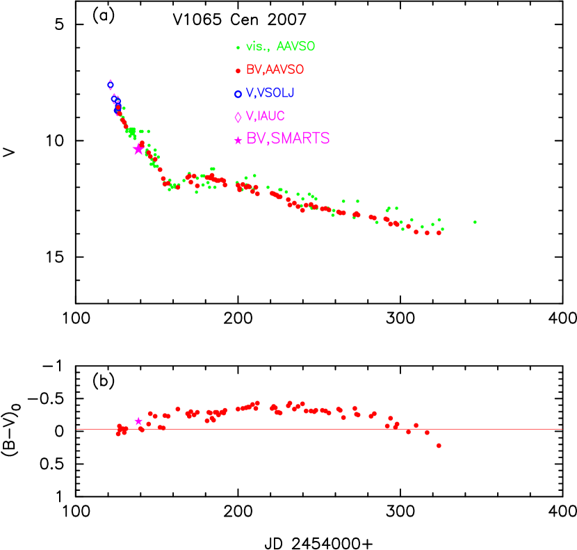
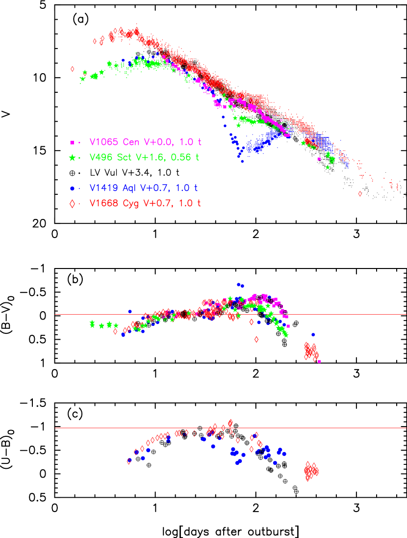
3.23. V1065 Cen 2007

This nova is not studied in Paper I. Figure 56 shows the visual and $V$ , and $(B-V)_{0}$ evolutions of V1065 Cen. The $BV$ data are taken from the AAVSO archive, and $V$ data are from the VSOLJ archive and IAU Circular Nos. 8800 and 8801. V1065 Cen reached $m_{V,\rm max}=7.6\pm 0.2$ at maximum on UT 2007 January 21. Then it smoothly declined with $t_{2}=11$ and $t_{3}=26$ days (Helton et al., 2010). A shallow dust black out started about 30 days after the optical maximum. V1065 Cen was identified as a neon nova by Helton et al. (2010).

The reddening for V1065 Cen was obtained as $E(B-V)=0.50\pm 0.10$ (Helton et al., 2010) from an average of three estimates, i.e., $E(B-V)=(B-V)_{\rm max}-(B-V)_{0,\rm max}=0.52\pm 0.04-(0.23\pm 0.06)=0.29\pm 0.07$ , $E(B-V)=(B-V)_{t2}-(B-V)_{0,t2}=0.41\pm 0.05-(-0.02\pm 0.04)=0.43\pm 0.06$ , and $E(B-V)=0.79\pm 0.01$ from the Balmer decrement (H $\alpha$ /H $\beta$ ). Helton et al. (2010) also estimated the apparent distance modulus in the $V$ band as $(m-M)_{V}=7.6\pm 0.2-(-8.6\pm 0.5)=16.2\pm 0.6$ from the MMRD relation together with $t_{2}=11$ days. This gives a distance of $d=8.7^{+2.8}_{-2.1}$ kpc. Assuming that the intrinsic $(B-V)_{0}$ color evolution of V1065 Cen is identical with that for similar types of novae, i.e., LV Vul, V1668 Cyg, V1419 Aql, and V496 Sct, we obtain $E(B-V)=0.45\pm 0.05$ from Figure 57(b), which is consistent with the estimate of Helton et al.

Using the time-stretching method (Figure 57(a)), we estimate the apparent distance modulus in the $V$ band, i.e.,

$\displaystyle(m-M)_{V,\rm V1065~{}Cen}$	$\displaystyle=$	$\displaystyle 15.3$	(47)
	$\displaystyle=$	$\displaystyle(m-M+\Delta V)_{V,\rm V1668~{}Cyg}+2.5\log 1.0/1.0$	(48)
	$\displaystyle\approx$	$\displaystyle 14.6+(+0.7-0.0)+0.0=15.3$	(49)
	$\displaystyle=$	$\displaystyle(m-M+\Delta V)_{V,\rm LV~{}Vul}+2.5\log 1.0/1.0$	(50)
	$\displaystyle=$	$\displaystyle 11.9+(+3.4-0.0)+0.0=15.3$	(51)
	$\displaystyle=$	$\displaystyle(m-M+\Delta V)_{V,\rm V1419~{}Aql}+2.5\log 1.0/1.0$	(52)
	$\displaystyle\approx$	$\displaystyle 14.6+(+0.7-0.0)+0.0=15.3$	(53)
	$\displaystyle=$	$\displaystyle(m-M+\Delta V)_{V,\rm V496~{}Sct}+2.5\log 0.56/1.0$	(54)
	$\displaystyle\approx$	$\displaystyle 14.4+(+1.6-0.0)-0.625=15.375,$	(55)

where we use $(m-M)_{V,\rm V1668~{}Cyg}=14.6$ from Section 2.1, $(m-M)_{V,\rm LV~{}Vul}=11.9$ from Section 2.2, $(m-M)_{V,\rm V1419~{}Aql}=14.6$ from Section 3.13, and $(m-M)_{V,\rm V496~{}Sct}=14.4$ from Section 3.30. Then, we obtain the distance of $d=6.0$ kpc for $E(B-V)=0.45$ and $(m-M)_{V}=15.3$ .

Figure 51(d) shows various distance-reddening relations for V1065 Cen, $(l,b)=(293\fdg 9841,+3\fdg 6130)$ . Here we plot the distance-reddening relation given by Marshall et al. (2006), i.e., four nearby directions, $(l,b)=(293\fdg 75,3\fdg 75)$ denoted by open red squares, $(294\fdg 00,3\fdg 75)$ by filled green squares, $(293\fdg 75,3\fdg 50)$ by blue asterisks, and $(294\fdg 00,3\fdg 50)$ by open magenta circles. The closest ones are those denoted by filled green squares and open magenta circles. Although these two relations differ for $d\gtrsim 3$ kpc, our values of $d=6.0$ kpc and $E(B-V)=0.45$ are midway between them. Thus, we think our cross point is consistent with the relation of Marshall et al. The relation of Green et al. (2015) is not available for these galactic coordinates.

Using $E(B-V)=0.45$ and $(m-M)_{V}=15.3$ , we plot the color-magnitude diagram of V1065 Cen in Figure 53(c). The track of V1065 Cen almost follows that of LV Vul (solid magenta lines). Thus, we regard V1065 Cen as an LV Vul type in the color-magnitude diagram. This coincidence with LV Vul strongly supports our values of $(m-M)_{V}=15.3$ and $E(B-V)=0.45$ . We specify the starting point of dust blackout (Helton et al., 2010) at $(B-V)_{0}=-0.06$ and $M_{V}=-4.06$ , denoted by a large open blue square in Figure 53(c). Helton et al. (2010) pointed out that the nova entered the early nebular phase at $m_{V}\approx 12$ , about 70 days after maximum. We denote this phase by a large open red square, at $(B-V)_{0}=-0.35$ and $M_{V}=-3.42$ . This point is close to the two-headed red arrow.

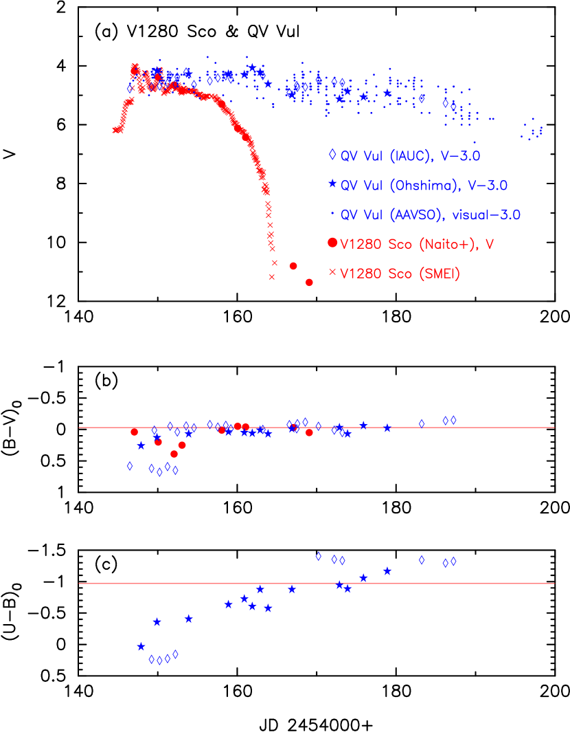
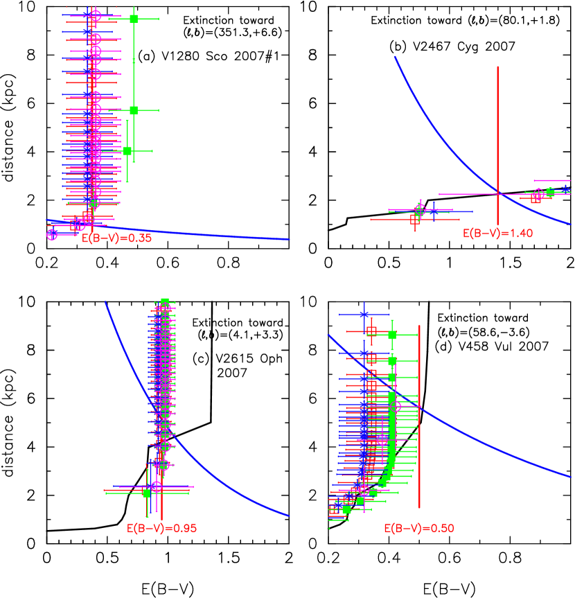
3.24. V1280 Sco 2007#1

This nova is not studied in Paper I. Figure 58 shows the $V$ and SMEI light curves and $(B-V)_{0}$ color evolution of V1280 Sco. The $UBV$ data for QV Vul (Figure 32) are added for comparison. The SMEI data for V1280 Sco are from Hounsell et al. (2010), and the $V$ data from Naito et al. (2012). V1280 Sco reached $m_{V,\rm max}=3.8$ at optical maximum on UT 2007 February 16.19 (Munari et al., 2007a). It experienced two major episodes of rebrightening peaking at UT February 16.15 and 19.18 (Hounsell et al., 2010). On UT February 26.4 its decline rate changed rapidly (e.g., Hounsell et al., 2010), indicating formation of an optically thick dust shell (Das et al., 2008).

The reddening for V1280 Sco was estimated by Das et al. (2008) as $E(B-V)=A_{V}/R_{V}=1.2/3.1\approx 0.4$ from Marshall et al.’s (2006) 3D dust map. The distance was obtained by Naito et al. (2012) as $d=1.1\pm 0.5$ kpc from the expansion parallax of a dust shell (Chesneau et al., 2008) together with the expansion velocity of $350\pm 160$ km s^-1.

In Figure 58(a), we shift the $V$ light curve of QV Vul up by 3.0 mag to fit its peak with that of V1280 Sco. In the early phase of these outbursts, the brightness shows similar fluctuations (both the amplitude and period). Therefore, we expect that the peak brightness is the same for V1280 Sco and QV Vul. Then we obtain the apparent distance modulus of $(m-M)_{V,\rm V1280~{}Sco}=(m-M)_{V,\rm QV~{}Vul}-3.0=14.0-3.0=11.0$ , where $(m-M)_{V,\rm QV~{}Vul}=14.0$ was already obtained in Section 3.11. We also determined that $E(B-V)=0.35$ by assuming that the intrinsic $(B-V)_{0}$ color is the same for both V1280 Sco and QV Vul (see Figure 58(b)). Then the distance is calculated as $d=0.96$ kpc for $E(B-V)=0.35$ and $(m-M)_{V}=11.0$ , being consistent with Naito et al.’s (2012) estimate of $d=1.1\pm 0.5$ kpc.

Figure 59(a) shows various distance-reddening relations for V1280 Sco, $(l,b)=(351\fdg 3311,+6\fdg 5534)$ . We plot Marshall et al.’s (2006) four relations, i.e., $(l,b)=(351\fdg 25,6\fdg 50)$ denoted by open red squares, $(351\fdg 50,6\fdg 50)$ by filled green squares, $(351\fdg 25,6\fdg 75)$ by blue asterisks, and $(351\fdg 50,6\fdg 75)$ by open magenta circles. The closer ones are those denoted by open red squares and filled green squares. The thick solid blue line indicates $(m-M)_{V}=11.0$ . These trends, i.e., Marshall et al.’s relations, $(m-M)_{V}=11.0$ , and $E(B-V)=0.35$ (vertical solid red line), cross at the point $d\approx 0.96$ kpc and $E(B-V)\approx 0.35$ . Thus we adopt $(m-M)_{V}=11.0$ and $E(B-V)=0.35$ .

Using $E(B-V)=0.35$ and $(m-M)_{V}=11.0$ , we plot the color-magnitude diagram of V1280 Sco in Figure 53(d). The track in the early phase looks similar to that of V705 Cas in Figure 37(b), although the peak brightness is $\sim 1$ mag fainter than that. We regard V1280 Sco as a V1668 Cyg type because the track goes down along that of V1668 Cyg. A large excursion toward red on the track in the early phase corresponds to the pulsation brightenings of the light curve. The dust formation occurred earlier when the nova was still in the brighter phase of the outburst (as indicated by a large open red square at $(B-V)_{0}=+0.01$ and $M_{V}=-5.70$ ) compared with other cases such as FH Ser and QV Vul.

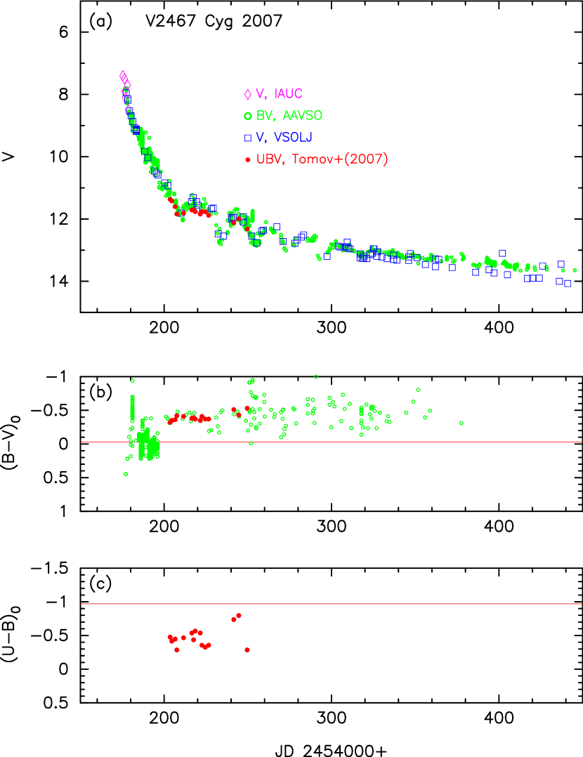
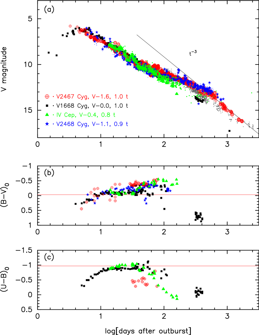
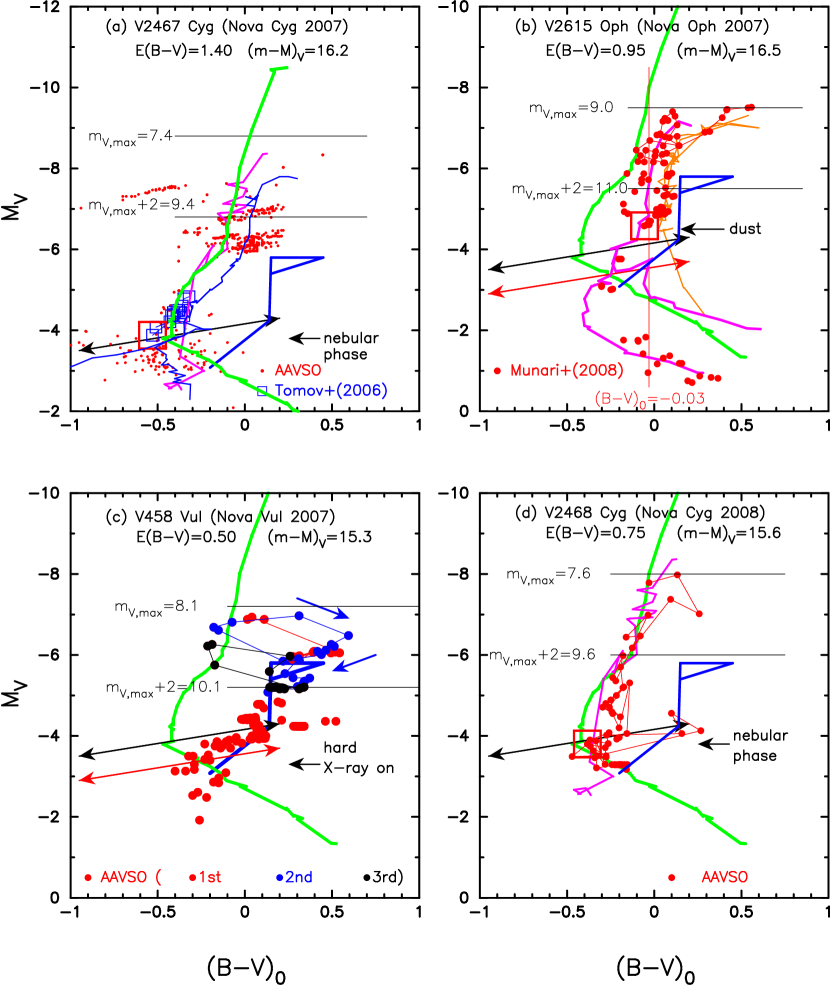
3.25. V2467 Cyg 2007

This nova is not studied in Paper I. Figure 60 shows the $V$ , $(B-V)_{0}$ , and $(U-B)_{0}$ evolutions of V2467 Cyg. The $UBV$ data of V2467 Cyg are taken from Tomov et al. (2007), $BV$ data from the AAVSO archive, and $V$ data from IAU Circular No. 8821, and the AAVSO and VSOLJ archives. V2467 Cyg smoothly declines with $t_{2}=7.6\pm 3.0$ and $t_{3}=14.6\pm 3.5$ days (e.g., Poggiani, 2009). Then the $V$ brightness shows some quasi-periodic oscillations with a period of 20–30 days and an amplitude of 0.7 mag during the transition phase as shown in Figure 60(a). These kinds of transition oscillations are similar to those of GK Per, V603 Aql, and V1494 Aql. The orbital period was estimated as $P_{\rm orb}=3.83$ hr (Shugarov et al., 2010). Swierczynski et al. (2010) suggested that V2467 Cyg is an intermediate polar with a spin period of 34.5 min.

The reddening and distance for V2467 Cyg were estimated as $E(B-V)=1.0$ –1.5 and $d\sim 2$ kpc (Steeghs et al., 2007) from the brightness and color of the progenitor, $E(B-V)=0.31$ (Munari et al., 2007b) from the Na I D2 equivalent width, $E(B-V)=1.5$ (Mazuk et al., 2007) from O I lines, and $E(B-V)=1.7$ (Russell et al., 2007) also from O I lines. In addition, the estimate $E(B-V)=1.16\pm 0.12$ and $d=2.6$ –3.6 kpc (Poggiani, 2009) came from $E(B-V)=(B-V)_{t2}-(B-V)_{0,t2}=1.14-(-0.02\pm 0.12)=1.16\pm 0.12$ and the distance modulus of $(m-M)_{V}=15.9$ –16.5, derived from various empirical relations of nova light curves, and $(m-M)_{V}=16.4\pm 0.2$ and $d=2.2\pm 0.2$ kpc (Hachisu & Kato, 2010) together with $E(B-V)=1.5$ (Mazuk et al., 2007) from their free-free model light curve fitting, and finally $E(B-V)=1.38\pm 0.12$ and $d=2.5\pm 0.3$ (Shugarov et al., 2010) from the absolute magnitude at maximum, $B-V$ color relations, and interstellar extinction.

We are not able to estimate the color excess from fitting in the color-color diagram because the $UBV$ data of V2467 Cyg obtained by Tomov et al. (2007) are for the transition oscillation phase, and hence inappropriate for the general track of novae, i.e., too late to derive the reddening. Using the time-stretching method for the light curves in Figure 61(a), we obtain the distance modulus in the $V$ band, i.e.,

$\displaystyle(m-M)_{V,\rm V2467~{}Cyg}$	$\displaystyle=$	$\displaystyle 16.2$	(56)
	$\displaystyle=$	$\displaystyle(m-M+\Delta V)_{V,\rm V1668~{}Cyg}-2.5\log 1.0/1.0$	(57)
	$\displaystyle\approx$	$\displaystyle 14.6+(-0.0+1.6)-0.0=16.2$	(58)
	$\displaystyle=$	$\displaystyle(m-M+\Delta V)_{V,\rm IV~{}Cep}-2.5\log 0.80/1.0$	(59)
	$\displaystyle\approx$	$\displaystyle 14.7+(-0.4+1.6)+0.24=16.14$	(60)
	$\displaystyle=$	$\displaystyle(m-M+\Delta V)_{V,\rm V2468~{}Cyg}-2.5\log 0.90/1.0$	(61)
	$\displaystyle\approx$	$\displaystyle 15.6+(-1.1+1.6)+0.11=16.21,$	(62)

where we use $(m-M)_{V,\rm V1668~{}Cyg}=14.6$ from Section 2.1, $(m-M)_{V,\rm IV~{}Cep}=14.7$ from Section 3.5, and $(m-M)_{V,\rm V2468~{}Cyg}=15.6$ from Section 3.28. Here, we squeeze the times of V2467 Cyg, IV Cep, and V2468 Cyg by a factor of 1.0, 0.80, and 0.90, and shift the $V$ light curves up by 1.6, 0.4, and 1.1 mag, respectively, against V1668 Cyg.

We also obtained $E(B-V)=1.40\pm 0.05$ by assuming that the intrinsic $(B-V)_{0}$ colors are similar among V2467 Cyg, V1668 Cyg, IV Cep, and V2468 Cyg as shown in Figure 61(b). Here, we de-reddened the $B-V$ and $U-B$ colors of V2467 Cyg with $E(B-V)=1.40$ .

Figure 59(b) shows various distance-reddening relations for V2467 Cyg, $(l,b)=(80\fdg 0690,+1\fdg 8417)$ . Here we plot the distance-reddening relations given by Marshall et al. (2006), i.e., $(l,b)=(80\fdg 00,2\fdg 00)$ denoted by open red squares, $(80\fdg 25,2\fdg 00)$ by filled green squares, $(80\fdg 00,1\fdg 75)$ by blue asterisks, and $(80\fdg 25,1\fdg 75)$ by open magenta circles. The closer ones are those denoted by open red squares and blue asterisks. We also added the distance-reddening relation given by Green et al. (2015). These four trends, i.e., Marshall et al.’s relations, Green et al.’s relation (solid black line), $(m-M)_{V}=16.2$ (thick solid blue line), and $E(B-V)=1.40$ (vertical solid red line), cross consistently at the point of $d\sim 2.4$ kpc and $E(B-V)\sim 1.40$ . Thus, we adopt $E(B-V)=1.40$ and $(m-M)_{V}=16.2$ .

Using $E(B-V)=1.40$ and $(m-M)_{V}=16.2$ , we plot the color-magnitude diagram of V2467 Cyg in Figure 62(a) as well as that of V1494 Aql (solid magenta line). The track of V2467 Cyg is very similar to those of V1500 Cyg and V1974 Cyg. Therefore, we regard V2467 Cyg as a V1974 Cyg type in the color-magnitude diagram. The nova entered the nebular phase at least on 2007 May 18, i.e., at $m_{V}=12.5$ (Poggiani, 2009). We specify a possible start of the nebular phase at the point of $(B-V)_{0}=-0.53$ and $M_{V}=-3.88$ as indicated by a large open red square in Figure 62(a).

3.26. V2615 Oph 2007

This nova is not studied in Paper I. Figure 63 shows the visual and $V$ , and $(B-V)_{0}$ evolutions of V2615 Oph on a linear timescale. The $BV$ data are taken from Munari et al. (2008a) and the AAVSO archive, $V$ data are from IAU Circular No. 8824, visual data are from the AAVSO archive. V2615 Oph reached $m_{V,\rm max}=9.0$ at optical maximum on UT 2007 March 25.48 (Munari et al., 2008a). Then it displayed an oscillatory behavior like PW Vul and gradually declined with $t_{2}=26.5$ and $t_{3}=48.5$ days (Munari et al., 2008a). A dust shell formed about 60 days after optical maximum to make a shallow dust blackout. The orbital period of 6.54 hr was detected by Mróz et al. (2015).

The reddening and distance for V2615 Oph were estimated as $E(B-V)=1.0$ –1.3 (Rudy et al., 2007a) from O I lines, as $E(B-V)=0.90$ and $d=3.7\pm 0.2$ kpc (Munari et al., 2008a) from an average of $E(B-V)=(B-V)_{\rm max}-(B-V)_{0,\rm max}=1.12-(0.23\pm 0.06)=0.89\pm 0.06$ and $E(B-V)=(B-V)_{t2}-(B-V)_{0,t2}=0.89-(-0.02\pm 0.04)=0.91\pm 0.04$ and from $(m-M)_{V}=15.7$ calculated by various empirical formulae including the MMRD and $M_{V,\rm 15}$ relations.

We plot the $V$ light curve and $B-V$ color evolution of V2615 Oph on a logarithmic timescale in Figure 64(a), as well as those of FH Ser, QV Vul, V705 Cas, and V475 Sct, because these light curves are very similar to each other. Since the timescales of these novae are almost the same, we regard that their brightnesses are the same as that of V2615 Oph. Then we obtain the apparent distance modulus of V2615 Oph as

$\displaystyle(m-M)_{V,\rm V2615~{}Oph}$	$\displaystyle=$	$\displaystyle 16.5$	(63)
	$\displaystyle=$	$\displaystyle(m-M+\Delta V)_{V,\rm FH~{}Ser}$	(64)
	$\displaystyle=$	$\displaystyle 11.7+(-0.0+4.8)=16.5$	(65)
	$\displaystyle=$	$\displaystyle(m-M+\Delta V)_{V,\rm QV~{}Vul}$	(66)
	$\displaystyle=$	$\displaystyle 14.0+(-2.3+4.8)=16.5$	(67)
	$\displaystyle=$	$\displaystyle(m-M+\Delta V)_{V,\rm V705~{}Cas}$	(68)
	$\displaystyle=$	$\displaystyle 13.4+(-1.7+4.8)=16.5$	(69)
	$\displaystyle=$	$\displaystyle(m-M+\Delta V)_{V,\rm V475~{}Sct}$	(70)
	$\displaystyle=$	$\displaystyle 15.4+(-3.7+4.8)=16.5,$	(71)

where we use $(m-M)_{V,\rm FH~{}Ser}=11.7$ from Section 2.3, $(m-M)_{V,\rm QV~{}Vul}=14.0$ from Section 3.11, $(m-M)_{V,\rm V705~{}Cas}=13.4$ from Section 3.14, and $(m-M)_{V,\rm V475~{}Sct}=15.4$ from Section 3.20. We also obtained $E(B-V)=0.95\pm 0.05$ by assuming that the intrinsic $(B-V)_{0}$ color of V2615 Oph are similar to those of FH Ser, QV Vul, and V705 Cas until the dust blackout started, as shown in Figure 64(b). The NASA/IPAC galactic dust absorption map gives $E(B-V)=0.87\pm 0.02$ in the direction toward V2615 Oph, being roughly consistent with our obtained value of $E(B-V)=0.95\pm 0.05$ . Thus, we adopt $E(B-V)=0.95\pm 0.05$ .

Figure 59(c) shows plot of various distance-reddening relations for V2615 Oph, $(l,b)=(4\fdg 1475,+3\fdg 3015)$ . Here we plot the distance-reddening relations given by Marshall et al. (2006), i.e., $(l,b)=(4\fdg 00,3\fdg 25)$ denoted by open red squares, $(4\fdg 25,3\fdg 25)$ by filled green squares, $(4\fdg 00,3\fdg 50)$ by blue asterisks, and $(4\fdg 25,3\fdg 50)$ by open magenta circles. The closest one is the one denoted by filled green squares. We also added the distance-reddening relation given by Green et al. (2015). These four trends, Marshall et al.’s relations, Green et al.’s relation (solid black line), $(m-M)_{V}=16.5$ (thick solid blue line), and $E(B-V)=0.95$ (vertical solid red line), consistently cross at $d=5.1$ kpc.

Using $E(B-V)=0.95$ and $(m-M)_{V}=16.5$ , we plot the color-magnitude diagram of V2615 Oph in Figure 62(b). The track of V2615 Oph is similar to that of FH Ser (solid orange lines) in the very early phase and then makes a loop clockwise near the track of LV Vul (solid magenta lines), corresponding to the oscillatory feature of the $V$ light curve, and then goes down along the track of FH Ser. However, note that there are two different $B-V$ color data sets in Munari et al. (2008a) from JD 2454220 to JD 2454250 as shown in Figure 63(b). Between $M_{V}=-6$ and $-4$ in Figure 62(b), one goes down along the track of FH Ser i.e., $(B-V)_{0}\sim+0.06$ , and the other goes down along that of LV Vul, i.e., $(B-V)_{0}\sim-0.10$ , until the dust-blackout started. These two different $B-V$ color data set were obtained at two different observatories, so we suppose that the response functions of the $V$ filters differ between them. After the recovery of the dust blackout, the V2615 Oph data follows those of LV Vul (magenta thick solid). If we adopt the redder side data, we regard V2615 Oph as a FH Ser type in the color-magnitude diagram. A dust shell was formed when the brightness declined to $m_{V}=12.0$ (Rudy et al., 2007a) as indicated by a large open red square in Figure 62(b). We specify this starting point by $(B-V)_{0}=-0.06$ and $M_{V}=-4.58$ .

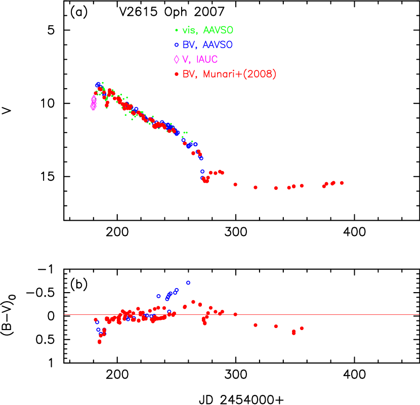
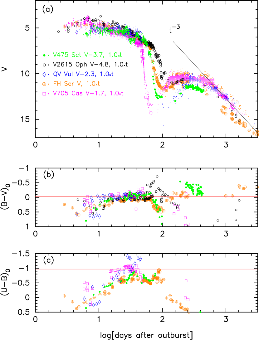
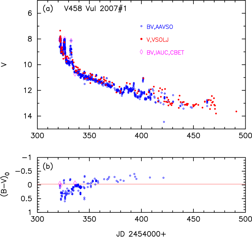
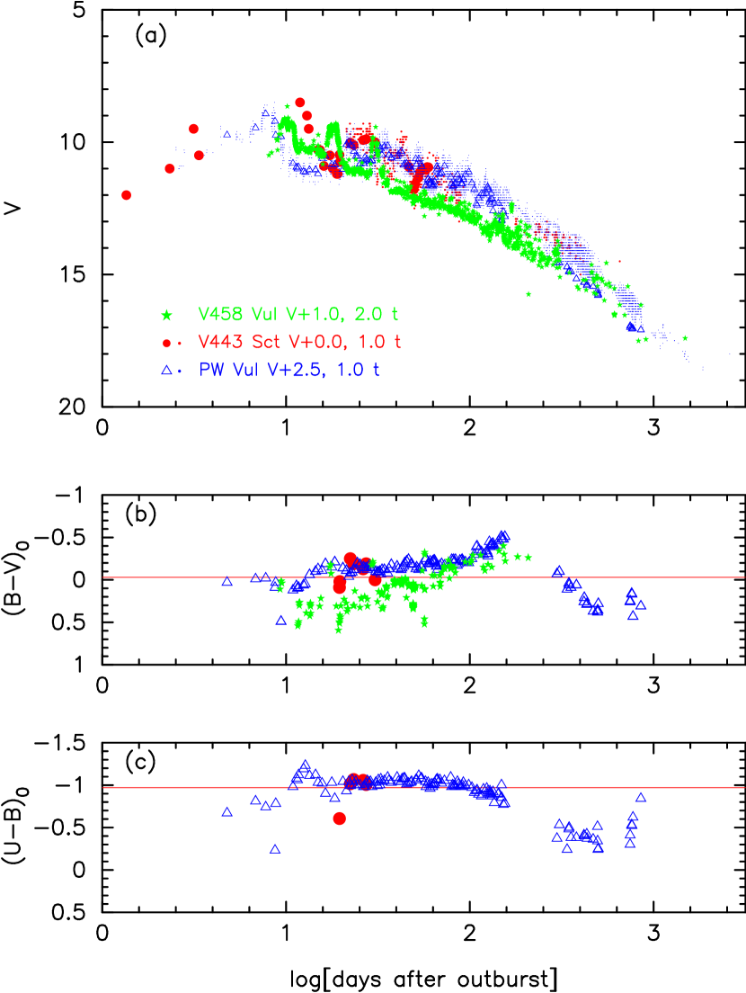
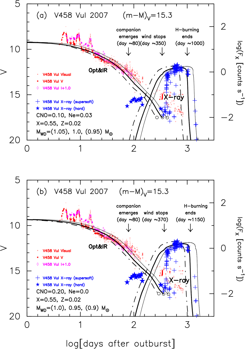
3.27. V458 Vul 2007#1

This nova is not studied in Paper I. Figure 65 shows the $V$ and $(B-V)_{0}$ evolutions of V458 Vul on a linear timescale. The $BV$ data are taken from IAU Circular No. 8863, CBET No. 1029, and the AAVSO archive. The $V$ data are from VSOLJ and IAU Circular Nos. 8861 and 8899, CBET Nos. 1029 and 1035. V458 Vul reached $m_{V,\rm max}=8.1$ at optical maximum on August 9.43 UT (Tarasova, 2007). Subsequently, it underwent two major rebrightenings with an amplitude of one magnitude on August 13.5 UT and August 19.5 UT. Then it declined with $t_{2}=8$ and $t_{3}=21$ days (e.g., Wesson et al., 2008), showing small amplitude fluctuations.

We also plot the light curve and color evolutions of V458 Vul on a logarithmic timescale in Figure 66 together with V443 Sct and PW Vul. The shape of the light curve and color evolution of V458 Vul are similar to those of V443 Sct and PW Vul. In the figure, we stretch the time of V458 Vul by a factor of 2.0 and shift the $V$ light curve down by 1.0 mag in order to make them overlap. In Paper I, we determined the apparent distance modulus of V458 Vul as $(m-M)_{V}=15.5$ by the time-stretching method. We reanalyzed the data and obtained $(m-M)_{V}=15.3$ from Figure 66(a), i.e.,

$\displaystyle(m-M)_{V,\rm V458~{}Vul}$	$\displaystyle=$	$\displaystyle 15.3$	(72)
	$\displaystyle=$	$\displaystyle(m-M+\Delta V)_{V,\rm PW~{}Vul}-2.5\log 1.0/2.0$	(73)
	$\displaystyle\approx$	$\displaystyle 13.0+(+2.5-1.0)+0.75=15.25$	(74)
	$\displaystyle=$	$\displaystyle(m-M+\Delta V)_{V,\rm V443~{}Sct}-2.5\log 1.0/2.0$	(75)
	$\displaystyle\approx$	$\displaystyle 15.5+(+0.0-1.0)+0.75=15.25,$	(76)

where we use $(m-M)_{V,\rm PW~{}Vul}=13.0$ from Section 2.4 and $(m-M)_{V,\rm V443~{}Sct}=15.5$ from Section 3.12. Thus, we adopt $(m-M)_{V,\rm V458~{}Vul}=15.3$ in the present paper.

The reddening for V458 Vul was obtained as $E(B-V)=0.6$ (Lynch et al., 2007) from O I lines, as $E(B-V)=0.55\pm 0.12$ (Poggiani, 2008) from $E(B-V)=(B-V)_{t2}-(B-V)_{0,t2}=0.53-(-0.02\pm 0.12)=0.55\pm 0.12$ , as $E(B-V)=0.63$ (Wesson et al., 2008) from the Balmer line ratio H $\alpha$ /H $\beta$ of the south-west knot of the nebula associated with the nova. The NASA/IPAC galactic dust absorption map gives $E(B-V)=0.54\pm 0.03$ in the direction toward V458 Vul. We obtain the reddening of $E(B-V)=0.50\pm 0.05$ by assuming that the intrinsic $(B-V)_{0}$ color evolution of V458 Vul is similar to that of PW Vul as shown in Figure 66(b). Then the distance is calculated as $d=5.6$ kpc for $E(B-V)=0.50$ and $(m-M)_{V}=15.3$ .

The distance to V458 Vul was obtained as $d=6.7$ –10.3 kpc (Poggiani, 2008) from various MMRD relations for $t_{2}=7\pm 2$ and $t_{3}=15\pm 2$ days and $M_{V,\rm 15}$ magnitude, and $d=13$ kpc (Wesson et al., 2008) from the MMRD relation, galactic rotation, and light echo time of nearby nebula associated with the nova. It is well known that the MMRD and $M_{V,15}$ relations represent statistical tendencies and do not give correct brightness for individual novae. Roy et al. (2012) claimed that the nova could be as close as $d\sim 6.5$ kpc or more from an analysis of the H I cloud associated with the nova.

Figure 59(d) shows various distance-reddening relations for V458 Vul, $(l,b)=(58\fdg 6331,-3\fdg 6171)$ . Here we plot the distance-reddening relations given by Marshall et al. (2006), i.e., $(l,b)=(58\fdg 50,-3\fdg 50)$ denoted by open red squares, $(58\fdg 75,-3\fdg 50)$ by filled green squares, $(58\fdg 50,-3\fdg 75)$ by blue asterisks, and $(58\fdg 75,-3\fdg 75)$ by open magenta circles. The closer ones are those denoted by filled green squares and open magenta circles. We also plot the distance-reddening relation given by Green et al. (2015). These trends cross consistently at the point $E(B-V)=0.50$ and $d=5.6$ kpc.

Assuming $E(B-V)=0.50$ and $(m-M)_{V}=15.3$ , we plot the color-magnitude diagram of V458 Vul in Figure 62(c). The basic part of the track is close to that of PU Vul (thick solid blue lines). Therefore, we regard V458 Vul as a PU Vul type. This is consistent with the fact that this type of novae, including RR Pic, V723 Cas, HR Del, and V5558 Sgr, have multiple peaks (or flares) in the very early phase (see Kato & Hachisu, 2009, 2011, for the reason behind multiple flaring pulses). We connect the first maximum by red lines, second by blue lines, and third by black lines. V458 Vul moves clockwise in the color-magnitude diagram during these three pulses (Figure 65) as indicated by blue arrows. This is very similar to that of V5558 Sgr in Figure 11(d).

Finally, we revisit the model light curve analysis of V458 Vul, which was analyzed in our previous paper (Hachisu & Kato, 2010). After that study, the end of the supersoft X-ray phase of V458 Vul was reported (e.g., Schwarz et al., 2011), which enables us to determine the WD mass more accurately. Our new model light curves are presented in Figure 67. The detail of our numerical methods are described in Hachisu & Kato (2016). We add calculated supersoft X-ray fluxes together with the observational X-ray data (filled blue stars for the hard X-ray phase and blue plus symbols for the soft X-ray phase). The X-ray count rates are taken from the Swift web page. We think that the steep rise in the X-ray flux near 380 days after the outburst corresponds to the epoch when the optically thick winds stopped (see, e.g., Hachisu & Kato, 2010). The optical and near infrared (NIR) light curves of free-free emission depend mainly on the WD mass and weakly on the chemical composition of the envelope. For the chemical composition $X=0.55$ , $Y=0.30$ , $X_{\rm CNO}=0.10$ , $X_{\rm Ne}=0.03$ , and $Z=0.02$ (Ne nova 2) for a typical neon nova, we have a best fit model with $M_{\rm WD}=1.0~{}M_{\sun}$ (black thick solid line) among $0.95$ , $1.0$ , and $1.05~{}M_{\sun}$ WDs as shown in Figure 67(a). If we assume $X=0.55$ , $Y=0.23$ , $X_{\rm CNO}=0.20$ , and $Z=0.02$ (CO nova 4) for a typical carbon-oxygen nova, on the other hand, we have a best fit model with $M_{\rm WD}=0.95~{}M_{\sun}$ among 0.9, 0.95, and $1.0~{}M_{\sun}$ WDs as shown in Figure 67(b).

Our previous model was $M_{\rm WD}=0.95~{}M_{\sun}$ for the chemical composition of Ne nova 2 (see Figure 27 of Hachisu & Kato, 2010) or $M_{\rm WD}=0.93~{}M_{\sun}$ for the chemical composition of CO nova 4 (see Figure 26 of Hachisu & Kato, 2010). The $V$ light curve was fitted with the free-free emission model light curve and it gave a distance modulus of $(m-M)_{V}=17.0$ (see Equation (86) of Hachisu & Kato, 2010). Here, we revised this fitting using new estimates of the WD mass, $1.0~{}M_{\sun}$ and $0.95~{}M_{\sun}$ for Ne nova 2 and CO nova 4, respectively, and new distance modulus, $(m-M)_{V}=15.3$ , as shown in Figure 67(a) and 67(b). This is consistent with the end of hydrogen shell burning. We included the contribution from the photospheric emission (blackbody approximation) in the $V$ light curve model in addition to the free-free emission (see, e.g., Hachisu & Kato, 2015).

Hard X-rays from novae are considered to originate from internal shocks in the ejecta (e.g., Mukai & Ishida, 2001) or shocks between the ejecta and circumstellar matter that is fed by the cool wind from a red-giant companion (e.g., Sokoloski et al., 2006). Hachisu & Kato (2010) claimed that the hard X-ray emission from V458 Vul comes from the shock between the ejecta and the companion. If that is the case, we may observe hard X-rays when the companion appears out of the optically thick nova envelope. We again examine this possibility. The orbital period of V458 Vul was first reported as $P_{\rm orb}=0.589$ days by Goranskij et al. (2008), but was later revised to $P_{\rm orb}=0.0681$ days by Rodríguez-Gil et al. (2011). Assuming that the companion is a $0.6~{}M_{\sun}$ CO core (e.g., Wesson et al., 2008), we obtain a separation of $0.82~{}R_{\sun}$ for the primary of $M_{\rm WD}=1.0~{}M_{\sun}$ . Then the emergence time of the secondary from the optically thick nova envelope is recalculated as $\sim 80$ days after the outburst based on our new nova models. This emergence time of the companion is coincident with the start of the hard X-ray (filled blue stars) increase.

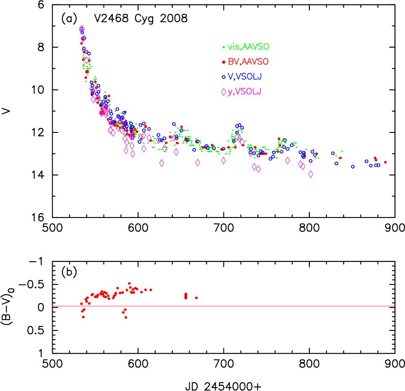
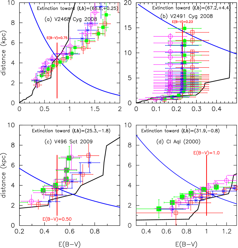
3.28. V2468 Cyg 2008#1

This nova is not studied in Paper I. Figure 68 shows the visual, $V$ , and $y$ light curves and $(B-V)_{0}$ color evolution of V2468 Cyg. The $BV$ data are taken from the AAVSO archive, and the $V$ and $y$ data are from the VSOLJ archive. V2468 Cyg reached $m_{V,\rm max}=7.6$ at optical maximum on UT 2008 March 9.5 (e.g., Chochol et al., 2012). Then it declined with $t_{2}=9$ and $t_{3}=20$ days, showing fluctuations with an amplitude of one magnitude and a period of a few days (Chochol et al., 2012). An orbital period of 3.49 hr was detected by Chochol et al. (2013).

The reddening for V2468 Cyg was obtained as $E(B-V)=0.77$ (Rudy et al., 2008a) from O I lines, $E(B-V)=0.80$ (Iijima & Naito, 2011) from hydrogen column density, $E(B-V)=0.8$ (Schwarz et al., 2009) from Balmer decrements, $E(B-V)=0.79\pm 0.01$ (Chochol et al., 2012) from a simple average of $E(B-V)=0.78$ from $E(B-V)=(B-V)_{t2}-(B-V)_{0,t2}=0.76-(-0.02\pm 0.04)=0.78$ , $E(B-V)=0.77$ from O I lines (Rudy et al., 2008a), $E(B-V)=0.8$ from the Balmer decrements (Schwarz et al., 2009), and $E(B-V)=0.80$ from the hydrogen column density (Iijima & Naito, 2011). These values are all consistent with each other, so we adopt $E(B-V)=0.75\pm 0.05$ in this paper.

The distance to V2468 Cyg was estimated mainly with the MMRD relations. Iijima & Naito (2011) estimated $(m-M)_{V}=m_{V,\rm max}-M_{V,\rm max}=7.3-(-8.8\pm 0.3)=16.1\pm 0.3$ from $t_{2}=7.8\pm 0.5$ days (della Valle & Livio, 1995) and calculated $d=5.5\pm 0.8$ kpc for $E(B-V)=0.8\pm 0.1$ . Chochol et al. (2012) also obtained $(m-M)_{V}=m_{V,\rm max}-M_{V,\rm max}=7.57-(-8.7\pm 0.07)=16.27\pm 0.07$ for $t_{2}=9$ days and $t_{3}=22$ days (della Valle & Livio, 1995; Downes & Duerbeck, 2000) and $d=5.4\pm 0.4$ kpc for $E(B-V)=0.79\pm 0.01$ .

In Paper I, we obtained the distance modulus of $(m-M)_{V}=15.6$ for V2468 Cyg by the time-stretching method. We confirmed this result of Paper I in Figure 55(a) and Equation (46), and also in Figure 61(a) and Equation (62). Assuming that the $(B-V)_{0}$ colors of V2468 Cyg, V1500 Cyg, V1668 Cyg, IV Cep, V2362 Cyg, and V2467 Cyg are very similar to each other, we obtain the color excess of V2468 Cyg $E(B-V)=0.75\pm 0.05$ as shown in Figures 55(b) and 61(b). This estimate is consistent with the previous results mentioned above.

Figure 69(a) shows various distance-reddening relations for V2468 Cyg, $(l,b)=(66\fdg 8084,+0\fdg 2455)$ . Here we plot the relations given by Marshall et al. (2006), i.e., $(l,b)=(66\fdg 75,0\fdg 00)$ denoted by open red squares, $(67\fdg 00,0\fdg 00)$ by filled green squares, $(66\fdg 75,0\fdg 25)$ by blue asterisks, and $(67\fdg 00,0\fdg 25)$ by open magenta circles. The closest one is denoted by blue asterisks. We also plot the distance-reddening relation given by Green et al. (2015). These distance-reddening relations cross at the same point, i.e., at the cross point of the two lines, $(m-M)_{V}=15.6$ (thick solid blue line) and $E(B-V)=0.75$ (vertical solid red line). The distance is calculated as $d=4.5$ kpc for $E(B-V)=0.75$ and $(m-M)_{V}=15.6$ .

Using $E(B-V)=0.75$ and $(m-M)_{V}=15.6$ , we plot the color-magnitude diagram of V2468 Cyg in Figure 62(d). The track of V2468 Cyg is similar to that of V1500 Cyg (thick solid green line). Therefore, we regard V2468 Cyg as a V1500 Cyg type in the color-magnitude diagram. The nova entered the nebular phase on UT 2008 July 8, about 125 days after the outburst, i.e., at $m_{V}=12.2$ (Iijima & Naito, 2011) as indicated by the large open red square at $(B-V)_{0}=-0.38$ and $M_{V}=-3.80$ in Figure 62(d).

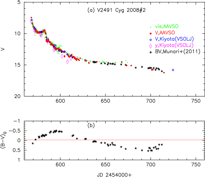
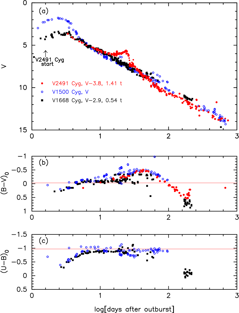
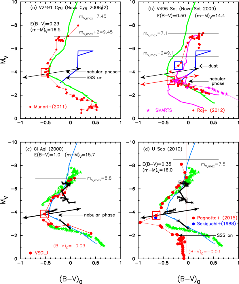
3.29. V2491 Cyg 2008#2

This nova is not studied in Paper I. Figure 70 shows the $y$ , $V$ , and visual light curves and $(B-V)_{0}$ color evolution of V2491 Cyg. This nova reached $m_{V,\rm max}=7.45\pm 0.05$ at optical maximum on UT 2008 April 11.37 (Munari et al., 2011). Then it declined with $t_{2}=4.8$ days, but rose again to $m_{V}=9.5$ about 15 days after maximum, which is the secondary maximum similar to those of V1493 Aql (Figure 40) and V2362 Cyg (Figure 54). Hachisu & Kato (2009) proposed a mechanism for the secondary maximum on the basis of a strong magnetic field on the WD. Although Page et al. (2010) discussed various X-ray properties of V2491 Cyg against a strong magnetic field, recently Zemko et al. (2015) found a 38 min periodicity and a possibility of a soft intermediate polar.

The reddening for V2491 Cyg was obtained as $E(B-V)=0.3$ (Lynch et al., 2008b) from O I lines, which was revised by Rudy et al. (2008b) to be $E(B-V)=0.43$ from the O I lines at 0.84 and $1.13~{}\mu$ m, and $E(B-V)=0.23\pm 0.01$ (Munari et al., 2011) from an average of $E(B-V)=0.24$ from Na I 5889.953 line profiles, $E(B-V)=(B-V)_{\rm max}-(B-V)_{0,\rm max}=0.46-(0.23\pm 0.06)=0.23\pm 0.06$ , and $E(B-V)=(B-V)_{t2}-(B-V)_{0,t2}=0.20-(-0.02\pm 0.04)=0.22\pm 0.04$ . The distance modulus and distance to V2491 Cyg were estimated by Munari et al. (2011) as $(m-M)_{V}=m_{V,\rm max}-M_{V,\rm max}=7.45-(-9.06)=16.51$ from the MMRD relation (Cohen, 1988) together with $t_{2}=4.8$ , and then derived as $d=14$ kpc. In this paper, we adopt $E(B-V)=0.23$ after Munari et al. because the $(B-V)_{0}$ color de-reddened with $E(B-V)=0.23$ almost overlaps the other color evolution curves of V1500 Cyg and V1668 Cyg as seen in Figure 71(b).

Using the time-stretching method (Figure 71(a)), we obtain the distance modulus of V2491 Cyg in the $V$ band

$\displaystyle(m-M)_{V,\rm V2491~{}Cyg}$	$\displaystyle=$	$\displaystyle 16.5$	(77)
	$\displaystyle=$	$\displaystyle(m-M+\Delta V)_{V,\rm V1500~{}Cyg}-2.5\log 1.0/1.41$	(78)
	$\displaystyle\approx$	$\displaystyle 12.3+(+0.0+3.8)+0.37=16.47$	(79)
	$\displaystyle=$	$\displaystyle(m-M+\Delta V)_{V,\rm V1668~{}Cyg}-2.5\log 0.54/1.41$	(80)
	$\displaystyle\approx$	$\displaystyle 14.6+(-2.9+3.8)+1.04=16.54$	(81)

where we use the apparent distance moduli of $(m-M)_{V,\rm V1500~{}Cyg}=12.3$ from Section 2.5 and $(m-M)_{V,\rm V1668~{}Cyg}=14.6$ from Sections 2.1.

Figure 69(b) shows various distance-reddening relations for V2491 Cyg, $(l,b)=(67\fdg 2287,+4\fdg 3531)$ . We plot the distance-reddening relations given by Marshall et al. (2006), i.e., $(l,b)=(67\fdg 00,4\fdg 25)$ denoted by open red squares, $(67\fdg 25,4\fdg 25)$ by filled green squares, $(67\fdg 00,4\fdg 50)$ by blue asterisks, and $(67\fdg 25,4\fdg 50)$ by open magenta circles. The closest one is that denoted by filled green squares. We also plot the distance-reddening relation given by Green et al. (2015). The extinction denoted by filled green squares nicely match the value of $E(B-V)=0.23$ . The NASA/IPAC galactic dust absorption map gives $E(B-V)=0.48\pm 0.03$ in the direction toward V2491 Cyg, being consistent with Green et al.’s relation. However, such large values of the reddening are inconsistent with those mentioned above. We obtain the cross point of the two trends, i.e., $(m-M)_{V}=16.5$ (thick solid blue line) and $E(B-V)=0.23$ (vertical solid red line), i.e., $d=14$ kpc at $E(B-V)=0.23$ .

Using $E(B-V)=0.23$ and $(m-M)_{V}=16.5$ , we plot the color-magnitude diagram of V2491 Cyg in Figure 72(a). V2491 Cyg is located very close to the track of V1500 Cyg. This similarity supports that our adopted values of $E(B-V)=0.23$ and $(m-M)_{V}=16.5$ ( $d=14$ kpc) are reasonable. Therefore, we regard V2491 Cyg as a V1500 Cyg type in the color-magnitude diagram. It is interesting that V1500 Cyg is also a strong magnetic system, a polar (Stockman et al., 1988). The nova possibly entered the nebular phase around $\sim 30$ days after maximum at $m_{V}=12.5$ (e.g., Munari et al., 2011; Tarasova, 2014). We specify the turning point $m_{V}\approx 12.5$ and $B-V=-0.28$ , i.e., $M_{V}\approx-4.0$ and $(B-V)_{0}=-0.51$ , denoted by a large open red square in Figure 72(a) and tabulated in Table 2. We add the epoch when the SSS phase started at $m_{V}=13.0$ , about 40 days after the outburst (Page et al., 2010).

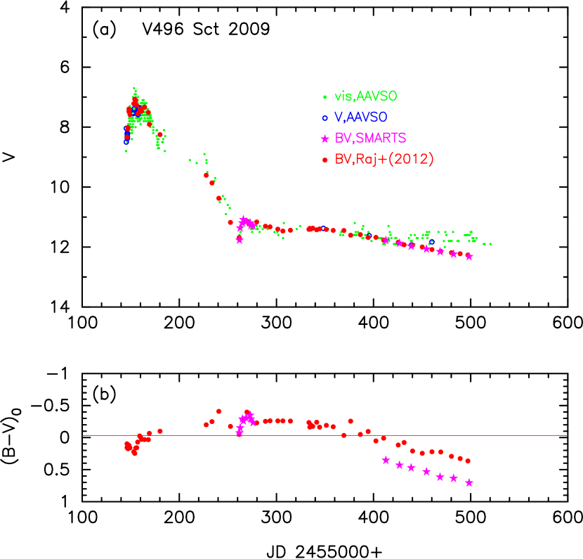
3.30. V496 Sct 2009

This nova is not studied in Paper I. Figure 73 shows the visual and $V$ , and $(B-V)_{0}$ evolutions of V496 Sct on a linear timescale. This nova reached $m_{V,\rm max}=7.07$ at optical maximum on UT 2009 November 18.716 (Raj et al., 2012). Then it declined with $t_{2}=59\pm 5$ days. There is lack of data between mid-December 2009 (JD 2455180) and early February 2010 (JD 2455220) due to a solar conjunction of V496 Sct. The $BV$ data are taken from Raj et al. (2012) (filled red circles) and the SMARTS archive (magenta stars) while the visual (green dots) and $V$ (open blue circles) data are from the AAVSO archive. It showed a shallow dip of dust shell formation about 90 days after optical maximum (e.g., Raj et al., 2012). Figure 73 has no $U-B$ color data because we could not find any $U$ band observation in the literature.

The reddening for V496 Sct was obtained by Raj et al. (2012) as $E(B-V)=(B-V)_{\rm max}-(B-V)_{0,\rm max}=0.797\pm 0.014-(0.23\pm 0.06)=0.57\pm 0.06$ from the intrinsic $B-V$ color at maximum and $E(B-V)=0.65$ from interstellar Na I line profile. They also estimated the distance modulus as $(m-M)_{V}=m_{V,\rm max}-M_{V,\rm max}=7.07-(-7.0\pm 0.2)=14.1$ from the MMRD relation (della Valle & Livio, 1995) together with $t_{2}=59$ and then derived $d=2.9\pm 0.3$ kpc.

Using the time-stretching method, we have already obtained $(m-M)_{V}=14.4$ as shown in Figure 57(a) together with Equation (55). The overall behavior of the V496 Sct $V$ light curve is similar to those of FH Ser and NQ Vul as shown in Figure 47(a). Assuming that these novae have the same brightness, we estimate the distance modulus as

$\displaystyle(m-M)_{V,\rm V496~{}Sct}$	$\displaystyle=$	$\displaystyle 14.4$	(82)
	$\displaystyle=$	$\displaystyle(m-M+\Delta V)_{V,\rm FH~{}Ser}-2.5\log 0.7$	(83)
	$\displaystyle=$	$\displaystyle 11.7+(+1.9+0.4)+0.39=14.39$	(84)
	$\displaystyle=$	$\displaystyle(m-M+\Delta V)_{V,\rm NQ~{}Vul}-2.5\log 0.7$	(85)
	$\displaystyle=$	$\displaystyle 13.6+(+0.0+0.4)+0.39=14.39,$	(86)

where we use $(m-M)_{V,\rm FH~{}Ser}=11.7$ from Sections 2.3 and $(m-M)_{V,\rm NQ~{}Vul}=13.6$ from Sections 3.6. The reddening is also estimated by assuming that the intrinsic $B-V$ color of V496 Sct is the same as that of FH Ser and NQ Vul. We obtain $E(B-V)=0.50\pm 0.05$ , as shown in Figure 47(b) and 57(b). We adopt $E(B-V)=0.50$ and $(m-M)_{V}=14.4$ . Then the distance is calculated to be $d=3.7$ kpc.

Figure 69(c) shows various distance-reddening relations for V496 Sct, $(l,b)=(25\fdg 2838,-1\fdg 7678)$ . We plot the distance-reddening relation given by Marshall et al. (2006), i.e., $(l,b)=(25\fdg 25,-1\fdg 75)$ denoted by open red squares, $(25\fdg 50,-1\fdg 75)$ by filled green squares, $(25\fdg 25,-2\fdg 00)$ by blue asterisks, and $(25\fdg 50,-2\fdg 00)$ by open magenta circles. The closest one is the one denoted by open red squares. We also plot the distance-reddening relation given by Green et al. (2015). Marshall et al.’s distance-reddening relation, denoted by open red squares, cross consistently our extinction of $E(B-V)\approx 0.50$ at $d\approx 3.7$ kpc.

Using $E(B-V)=0.50$ and $(m-M)_{V}=14.4$ , we plot the color-magnitude diagram of V496 Sct in Figure 72(b). The track of V496 Sct is very similar to that of LV Vul. This confirms that our values of $E(B-V)=0.50$ and $(m-M)_{V}=14.4$ are reasonable. Therefore, we regard V496 Sct as an LV Vul type in the color-magnitude diagram. The dust blackout started $\sim 90$ days after the outburst at $m_{V}\approx 9.9$ (e.g., Raj et al., 2012). We denote the start of the dust blackout by a large open blue square. The nebular phase possibly started $\sim 130$ days after the outburst at $m_{V}\approx 11.2$ (e.g., Raj et al., 2012). We specify it by a large open red square on the track, i.e., $(B-V)_{0}=-0.35$ and $M_{V}=-3.26$ .

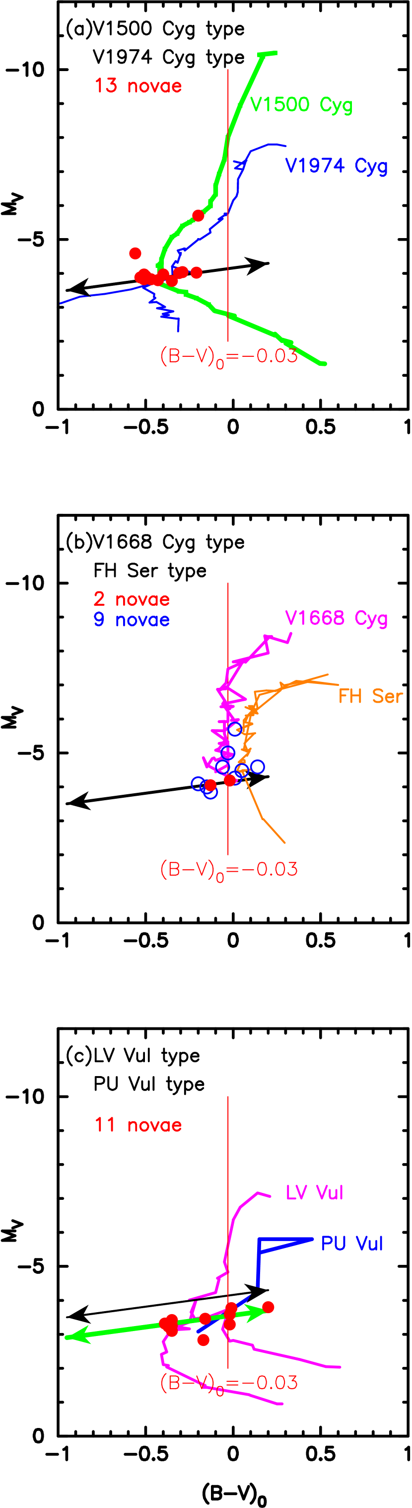
4. Discussion

4.1. Categorization of nova tracks

Figure 12 depicts the color-magnitude tracks of six templates, from left to right: V1500 Cyg (thick solid green), V1668 Cyg (magenta), V1974 Cyg (sky blue), LV Vul (black), FH Ser (orange), and PU Vul (blue). We have collected 40 nova tracks in the color-magnitude diagram (Figures 3, 6, 7, 11, 16, 23, 30, 37, 45, 53, 62, and 72), compared them with the template tracks in Figure 12, and categorized them into one of the six as listed in Table 2. The V1500 Cyg type includes 8 novae, i.e., V1500 Cyg, T Pyx, GQ Mus, V1494 Aql, V2275 Cyg, V2362 Cyg, V2468 Cyg, and V2491 Cyg, mainly fast novae. The V1974 Cyg type includes 7 novae, i.e., V1974 Cyg, V2467 Cyg, V533 Her, QU Vul, V1493 Aql, V382 Vel, and V5114 Sgr. The V1668 Cyg type includes 8 novae, i.e., V1668 Cyg, V446 Her, OS And, V705 Cas, V1419 Aql, V2274 Cyg, V475 Sct, and V1280 Sco. The FH Ser type includes 4 dust formation novae, i.e., FH Ser, NQ Vul, QV Vul, and V2615 Oph. The LV Vul type includes 8 novae, i.e., LV Vul, RS Oph, PW Vul, IV Cep, V443 Sct, V1370 Aql, V1065 Cen, and V496 Sct. The PU Vul type includes 5 novae, i.e., PU Vul, HR Del, V723 Cas, V5558 Sgr, and V458 Vul. Some of these novae show a hybrid signature, e.g., V1065 Cen evolved along the path of V1668 Cyg in the early phase until $M_{V}\sim-4$ and then followed LV Vul as shown in Figure 53(c). In this paper, therefore, we put V1065 Cen into the LV Vul type, although V1065 Cen underwent a shallow dust blackout like V1668 Cyg.

The different $B-V$ color position of each track in the color-magnitude diagram can be understood as a difference in the envelope mass. In general, novae on the bluer side have smaller envelope masses. For example, the V1500 Cyg and V1974 Cyg types differ in the $B-V$ color as shown in Figure 74(a). This color difference originates from the difference in the envelope mass, i.e., V1500 Cyg has a less massive envelope and evolves more rapidly (e.g., $M_{\rm env}=0.53\times 10^{-5}M_{\sun}$ for a $1.2~{}M_{\sun}$ WD model of V1500 Cyg versus $M_{\rm env}=1.2\times 10^{-5}M_{\sun}$ for a $0.98~{}M_{\sun}$ WD model of V1974 Cyg in Hachisu & Kato, 2016). A good example of this difference can be seen in the track of V2362 Cyg. In the early decline phase, V2362 Cyg evolves downward along the track of FH Ser until $M_{V}\sim-4$ , as depicted by filled red circles in Figure 53(b). After that, the $V$ magnitude rises up to the secondary maximum ( $M_{V}\sim-6$ ) and sharply drops down to $M_{V}\sim-2$ , as depicted by open magenta circles. A large amount of envelope mass was lost during this secondary maximum (Munari et al., 2008b). The position of the secondary maximum in the color-magnitude diagram is about 0.2 mag bluer than that of the first maximum. This track shift toward blue is caused by the loss of envelope mass.

The difference between the V1668 Cyg and FH Ser types shown in Figure 74(b) can also be understood as a difference in envelope mass. Both types have a dust formation episode, but the dust blackout is much shallower in the V1668 Cyg type than in the FH Ser type. This indicates that the envelope mass is more massive in the FH Ser type novae.

In PW Vul, a massive envelope could be ejected during the very early phase as represented by a large clockwise circle in the color-magnitude diagram (e.g., Kolotilov & Noskova, 1986). After that, it follows a track similar to that of LV Vul in the mid and late decline phase. Such a shift toward blue is also observed in the multiple peaks of V5558 Sgr (Figure 11(d)). This also suggests a large decrease in the envelope mass.

4.2. Absolute magnitude at nebular phase

The color-magnitude diagram (HR diagram) is an excellent tool for understanding the nature of stars (e.g., their evolution and absolute magnitudes), but it has not yet been widely applied to nova outbursts. In Paper I, we discussed a new way to estimate the distance to a nova. The method in Paper I was as follows: (1) we first determine $E(B-V)$ by fitting the color-color evolution of a target nova with the general course of novae, (2) choose a reference nova with known distance and extinction and compare it with our target nova, (3) obtain $(m-M)_{V}$ by the time-stretching method of light curves, i.e., using the relation $m^{\prime}_{V}=m_{V}-2.5\log f_{s}$ (Hachisu & Kato, 2010), and (4) calculate the distance with Equation (3).

Here, we propose another new method based on the type of nova tracks and the starting points of the nebular phase in the color-magnitude diagram. Figure 74 summarizes the positions of starting points of the nebular phase or dust blackout of each nova in the color-magnitude diagram. In the V1500 Cyg and V1974 Cyg type novae, i.e., the V1500 Cyg family, the gradual change toward blue in the very early phase ( $M_{V}<-6$ ) corresponds to continuum free-free emission phase of the nova spectrum. Then some emission lines become stronger in the $B$ band. The contribution of these emission lines causes an excursion toward blue between $-6<M_{V}<-4$ . After the turning point near $M_{V}\sim-4$ , it went toward red due to a large contribution of emission lines [O III] to the $V$ -band. This turning point (or cusp) can be clearly identified in many of the V1500 Cyg family novae. We found that the start of the nebular phase almost coincides with the turning point (or cusp) and are already showing its position as a large red square in each color-magnitude diagram. We plot this turning point (or cusp) as an indication of the development of the nebular stage by filled red circles in Figure 74(a). These filled red circles are located on the two-headed black arrow of Equation (5) except for two novae, T Pyx and GQ Mus.

For the V1668 Cyg and FH Ser types of novae, i.e., the V1668 Cyg family, they often show a dust blackout at $M_{V}\sim-4.5$ before the above excursion toward red or blue. We plot the starting points of the dust blackout by open blue circles in Figure 74(b). They are rather scattered. On the other hand, we plot the starting points of nebular phase by filled red circles for the two novae V1668 Cyg and V446 Her. These points are located on the two-headed arrow of Equation (5). The filled red circles in Figure 74(a) and 74(b) are located on the two-headed arrows represented by Equation (5) except for T Pyx and GQ Mus. Inversely, we obtain Equation (5) from these 13 red points, excluding T Pyx and GQ Mus.

The LV Vul and PU Vul type novae, i.e., the LV Vul family, have slightly different starting positions for the nebular phase. We plot also the starting points for the LV Vul family novae in Figure 74(c) by filled red circles. They are located on the two-headed green arrow represented by Equation (6), which is 0.6 mag below the two-headed black arrow represented by Equation (5). We obtained this lower line from these 11 red points in Figure 74(c).

In this way, we found the characteristic epochs corresponding to a certain magnitude given by Equation (5) or (6). Using this property, we are able to obtain the absolute magnitude of the target nova by placing the starting point of the nebular phase on the line of Equation (5) or Equation (6) depending on the nova type. This is a new method for determining the absolute magnitude of a nova.

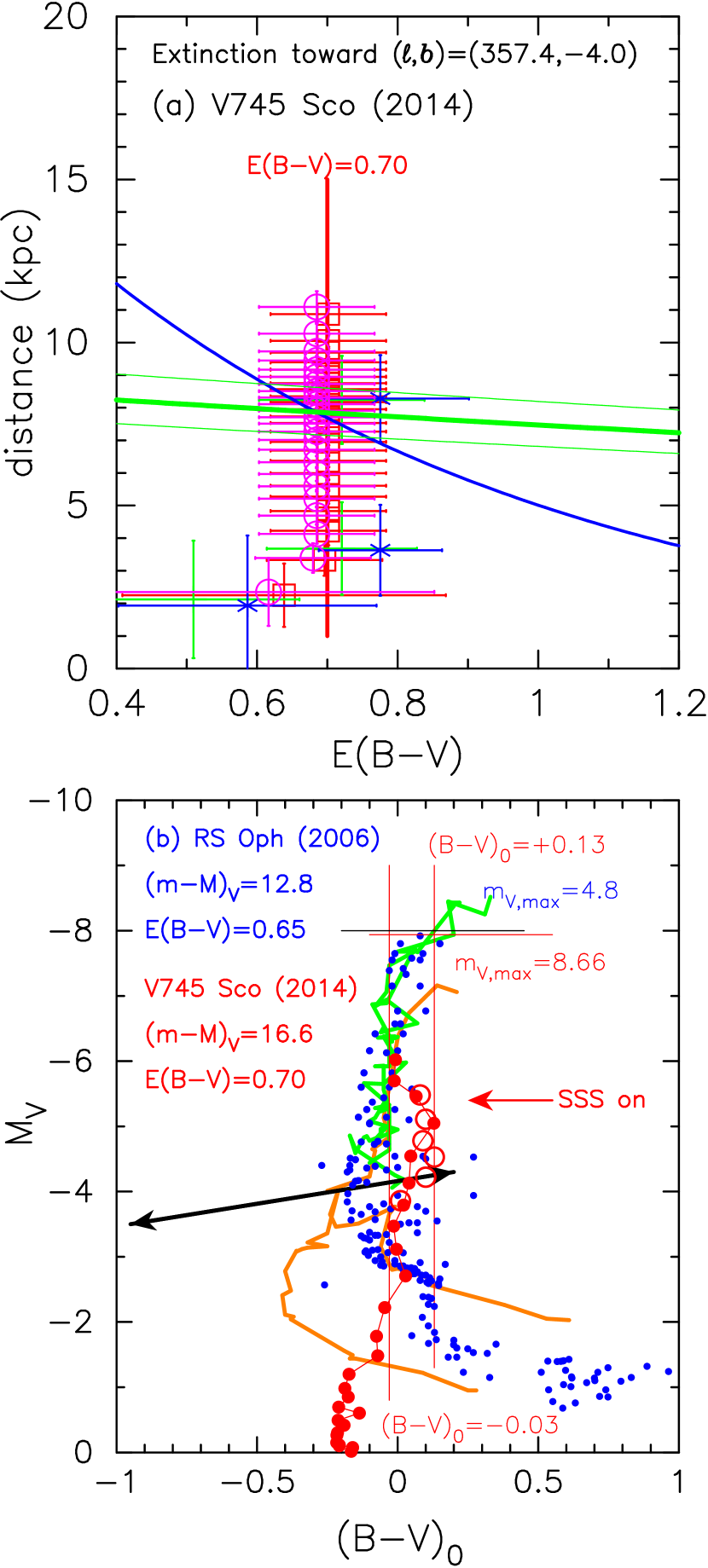
4.3. Application to recurrent novae

Using the color-magnitude diagram method summarized above in Section 4.2, we can estimate the absolute magnitudes of novae. This is essentially the same method as the main-sequence fitting or horizontal-branch fitting in the HR diagram to estimate the distances to star clusters. In this subsection, we first confirm our method by applying it to the M31 1 yr recurrent nova, M31N 2008-12a, and then estimate the absolute magnitudes of three well-observed recurrent novae, CI Aql, U Sco, and V745 Sco.

4.3.1 M31N 2008-12a

The 1 yr recurrence period nova M31N 2008-12a is an excellent example of a recurrent nova because the distance and extinction are well determined (Darnley et al., 2015; Henze et al., 2015; Kato et al., 2015). The nova has $t_{2}=1.77$ days and $t_{3}=3.84$ days in the $V$ band (Darnley et al., 2015), being a very fast nova. Kato et al. (2015) concluded, on the basis of their multi-wavelength light curve model, that the WD mass is close to $1.38~{}M_{\sun}$ . The distance to M31 is $d\approx 780$ kpc and the extinction is $E(B-V)\approx 0.21$ toward the nova (e.g., Henze et al., 2015). Then the distance modulus is calculated to be $(m-M)_{V}=25.1$ .

Adopting $E(B-V)=0.21$ and $(m-M)_{V}=25.1$ , we plot the color-magnitude diagram of M31N 2008-12a in Figure 72(c) and 72(d) by open black squares with connected solid black lines. The data for the 2014 outburst are taken from Darnley et al. (2015) and for the 2015 outburst from ATel Nos. 7974, 7965, 7967, 7969, 8033, 8029, and 8038. The peak brightness is about $M_{V}\approx-6.6$ , much fainter than typical classical novae. Darnley et al. (2015) estimated that the peak brightness is $-6.8<M_{V}<-6.3$ . The nova almost goes down along the line of $(B-V)_{0}=-0.03$ in the early phase, then turns to the left (toward blue) in the middle phase, and comes back to the right in the later phase. The turning point is not clearly identified but possibly located near the two-headed arrow. This supports our method of absolute magnitude determination discussed in the previous subsection (Section 4.2).

4.3.2 CI Aql

CI Aql is also a recurrent nova with recorded outbursts in 1917, 1941, and 2000. Schaefer (2001c) proposed that CI Aql could have an outburst every $\sim 20$ yr. Kiss et al. (2001) estimated the reddening of CI Aql $E(B-V)=0.85\pm 0.3$ from an average of various methods. Hachisu & Kato (2001a), Hachisu et al. (2003), and Lederle & Kimeswenger (2003) derived $E(B-V)\approx 1.0$ based on their binary model light curve fittings. Lynch et al. (2004) obtained $E(B-V)=1.5\pm 0.1$ from the O I line ratios. Iijima (2012) obtained $E(B-V)=0.92\pm 0.15$ from the equivalent widths of the diffuse interstellar absorption bands.

Figure 72(c) shows the data of CI Aql (filled red circles connected with a solid red line), taken from the VSOLJ archive (mainly from Kiyota’s data). Iijima (2012) found that CI Aql entered the nebular phase between UT 2000 May 31 and June 8 at $m_{V}\approx 11.8$ . We identify a turning point (or cusp) at the starting point of the nebular phase, i.e., at the point $(B-V)_{0}=-0.52$ and $M_{V}=-3.84$ (large open red square). Adopting $E(B-V)=1.0$ , we obtain the distance modulus in the $V$ band from a fit with Equation (5). The derived distance modulus is $(m-M)_{V}=11.9-(-3.8)=15.7$ at the turning point. We can regard CI Aql as a V1500 Cyg type in the color-magnitude diagram, so the fit with Equation (5) is justified. We plot the track of V1500 Cyg by thick solid sky-blue lines and that of the recurrent nova T Pyx by green stars in Figure 72(c). The track of CI Aql almost follows these trends. This also confirms that our adopted values of $E(B-V)=1.0$ and $(m-M)_{V}=15.7$ are reasonable.

The distance is then calculated to be $d\approx 3.3$ kpc. This value is shorter than the $\sim 5.0$ kpc obtained by Schaefer (2010) from the MMRD relation (Downes & Duerbeck, 2000), but longer than the value of $d\sim 1.5$ kpc estimated from the blackbody binary model light curves (Hachisu & Kato, 2001a; Hachisu et al., 2003; Lederle & Kimeswenger, 2003) together with $E(B-V)=1.0$ . In general, one should not use the MMRD relations to obtain the maximum magnitudes of recurrent novae because they are faint objects as already discussed in our previous papers (Hachisu & Kato, 2010, 2014, 2015, 2016). Sahman et al. (2013) obtained $d=1.3\pm 0.2$ kpc from the spectral type (F8IV) of the companion star together with Lynch et al.’s estimate of $A_{V}=4.6\pm 0.5$ . If we adopt $E(B-V)=1.0$ ( $A_{V}=3.1$ ), Sahman et al.’s distance could be larger than $d\gtrsim 2.6$ kpc.

The set $d=3.3$ kpc and $E(B-V)=1.0$ is consistent with the distance-reddening relations for CI Aql, $(l,b)=(31\fdg 6876,-0\fdg 8120)$ , in Figure 69(d). Here, we plot $(m-M)_{V}=15.7$ , $E(B-V)=1.0$ , and four nearby distance-reddening relations given by Marshall et al. (2006), i.e., $(l,b)=(31\fdg 50,-0\fdg 75)$ denoted by open red squares, $(31\fdg 75,-0\fdg 75)$ by filled green squares, $(31\fdg 50,-1\fdg 00)$ by blue asterisks, and $(31\fdg 75,-1\fdg 00)$ by open magenta circles. The closest one is that of the filled green squares. We also add the relation (solid black line) given by Green et al. (2015). These trends cross consistently at $d\approx 3.3$ kpc and $E(B-V)\approx 1.0$ .

To summarize, the color-magnitude track of CI Aql almost overlaps with the tracks of T Pyx and V1500 Cyg and its distance-reddening relation is consistent with the Marshall et al. relation. Thus, we may conclude that the set of $E(B-V)=1.0$ and $(m-M)_{V}=15.7$ ( $d\approx 3.3$ kpc) is reasonable. We summarize the results in Table 3.

4.3.3 U Sco

U Sco is also a recurrent nova with ten recorded outbursts in 1863, 1906, 1917, 1936, 1945, 1969, 1979, 1987, 1999, and 2010, almost every ten years (Schaefer, 2010). It is located at a high galactic latitude, $(l,b)=(357\fdg 6686,+21\fdg 8686)$ . Thus, it is far from the galactic plane ( $z>1$ kpc) if its distance is large enough ( $d\gtrsim 3$ kpc), as suggested in the literature. Therefore, the extinction for U Sco should be close to the galactic dust extinction. The NASA/IPAC galactic dust absorption map gives $E(B-V)=0.32\pm 0.04$ for U Sco. Unfortunately, direct measurements of reddening show a scatter between 0.1 and 0.35 (e.g., Schaefer, 2010). For example, Barlow et al. (1981) obtained two different absorptions toward U Sco in the 1979 outburst, $E(B-V)\sim 0.2$ from the line ratio of He II at an early phase of the outburst ( $\sim 12$ days after maximum) and $E(B-V)\sim 0.35$ from the Balmer line ratio at a late phase of the outburst ( $\sim 33$ —34 days after maximum). The latter value is consistent with that of the galactic dust absorption map.

Adopting $E(B-V)=0.35$ , we plot the color-color diagram of the U Sco 2010 outburst in Figure 36(c). The $B-V$ and $U-B$ color data are taken from Pagnotta et al. (2015). The track of U Sco almost overlaps with the general track of novae (solid green lines) in the color-color diagram. Thus, we confidently determine the reddening of U Sco as $E(B-V)=0.35\pm 0.05$ .

Figure 72(d) shows the color-magnitude diagram of U Sco. Here we adopt $E(B-V)=0.35$ and then determine the distance modulus in the $V$ band from the fit with Equation (5). We identify a turning point (or cusp) at the point $(B-V)_{0}=-0.64$ and $M_{V}=-3.72$ (large open red square) as shown in Figure 72(d). The distance modulus is then calculated to be $(m-M)_{V}=12.3-(-3.7)=16.0$ at the turning point (large open red square). Then the peak is as bright as $M_{V,\rm max}=7.5-16.0=-8.5$ , about 0.5 mag brighter than the peaks of RS Oph and T Pyx (see Figure 16(a) and 16(d)), and 1.5 mag brighter than the peak of CI Aql (Figure 72(c)). After the turning point (large open red square), U Sco goes down further, crossing the two-headed arrow, and jumps to the left (toward blue) up to $(B-V)_{0}\sim-1.0$ . We neglect this bluest point in our determination of the turning point, because it could be affected by the first flare in the 2010 outburst (e.g., Schaefer, 2011; Maxwell et al., 2012; Anupama et al., 2013; Pagnotta et al., 2015). Below $M_{V}>-3.0$ , we suppose that the $B$ and $V$ magnitudes are affected by a large irradiated disk around the WD (e.g., Hachisu et al., 2000a) and, as a result, the $B-V$ color is contaminated by the disk radiation. This is the reason why the color-magnitude track of U Sco stays at $(B-V)_{0}\approx-0.1$ between $-2.0\lesssim M_{V}\lesssim-0.0$ . We added the epoch when the SSS phase started at $m_{V}=14.0$ , about 14 days after the outburst (Schaefer et al., 2011).

The distance to U Sco is calculated to be $d=9.6\pm 0.6$ kpc. This is larger than the $d=6$ –7 kpc calculated from the nova explosion/quiescent models of Hachisu et al. (2000a, b). Assuming totality at mid-eclipse, Schaefer (2010) proposed a larger value of $d=12\pm 2$ kpc estimated from the spectral type (G5IV) of the companion star. We should note that a different spectral type (K2IV) of the companion was proposed by Anupama & Dewangan (2000). Anupama et al. (2013) revised their spectral type to K0 $\sim$ K1. Mason et al. (2012) proposed that the spectral type of the secondary star is not earlier than F3 and not later than G, but concluded that they cannot confidently exclude an early K spectral type for U Sco. Thus, we must be careful with the distance determination from only the spectral type of the secondary. We summarize our results in Table 3.

We added the $B-V$ and $U-B$ color evolution of T Pyx (1966) in Figure 36(c) by filled blue circles. The data are the same as those in Figure 30(a) of Paper I. The color-color evolutions of U Sco (2010) and T Pyx (1966) overlap each other. The color-magnitude track of U Sco (filled red circles connected by solid red line) in Figure 72(d) follows that of T Pyx (green stars) in the early phase. The color-color and color-magnitude evolutions of U Sco are very similar to those of T Pyx.

Table 3Physical properties of selected recurrent novae

Object	$E(B-V)$	$(m-M)_{V}$	Distance	$M_{V,\rm max}$	$P_{\rm orb}$	RN type^a^aRecurrent novae (RNe) are divided into three types, depending on the nature of the companion (or the orbital period), i.e., T Pyx ( $P_{\rm orb}\sim$ a few hours), U Sco ( $P_{\rm orb}\sim$ a day), and RS Oph ( $P_{\rm orb}\sim$ a few to several hundred days) types (e.g., Anupama, 2008).
			(kpc)		(day)
RS Oph	$0.65$	$12.8$	$1.4$	$-8.0$	$457$ ^b^btaken from Fekel et al. (2000).	RS Oph
T Pyx	$0.25$	$14.2$	$4.8$ ^c^ctaken from Sokoloski et al. (2013).	$-7.9$	$0.076$ ^d^dtaken from Uthas et al. (2010).	T Pyx
CI Aql	$1.0$	$15.7$	$3.3$	$-6.9$	$0.618$ ^e^etaken from Mennickent & Honeycutt (1995).	U Sco
U Sco	$0.35$	$16.0$	$9.6$	$-8.5$	$1.23$ ^f^ftaken from Schaefer & Ringwald (1995).	U Sco
V745 Sco	$0.70$	$16.6$	$7.8$	$-7.9$	—	RS Oph

4.3.4 V745 Sco

V745 Sco is also a recurrent nova with three recorded outbursts, in 1937, 1989, and 2014. Figure 75 shows the $V$ light curve, supersoft X-ray count rate, $(B-V)_{0}$ , and $(U-B)_{0}$ color evolutions of V745 Sco for the 1989 and 2014 outbursts. The $UBV$ data of the 1989 outburst are taken from Sekiguchi et al. (1990) and the $BV$ and X-ray data of the 2014 outburst are from Page et al. (2015). If the 2014 outburst is the same as the 1989 outburst, the $V$ magnitude (open blue circles) of Sekiguchi et al. (1990) are systematically 0.3 mag brighter than those (filled red circles) of Page et al. (2015). Therefore, we shift the $V$ magnitudes down by 0.3 mag and confirm that these two $V$ light curves overlap each other as shown in Figure 75(a). Such a difference among observers was already discussed in our previous sections and attributed to slightly different responses of the $V$ filters. When Sekiguchi et al. started $UBV$ photometry about four days after the outburst; the supersoft X-ray source (SSS) phase just began, indicating that the ejecta had already become optically thin. The spectra of the 1989 outburst show that the nebular [O III] lines had already developed at this time (e.g.,, Duerbeck, 1989). If we shift Sekiguchi et al.’s $V$ down by 0.3 mag, then Sekiguchi et al.’s $(B-V)_{0}$ data are consistently overlapping those of Page et al. as shown in Figure 75(b). The 2014 outburst shows $t_{2}=2$ and $t_{3}=4$ days (e.g., Orio et al., 2014).

The galactic coordinates of V745 Sco is $(l,b)=(357\fdg 3584,-3\fdg 9991)$ . The NASA/IPAC galactic dust absorption map gives $E(B-V)=0.71\pm 0.02$ for V745 Sco. Banerjee et al. (2014) suggested that the extinction for V745 Sco is $E(B-V)=0.70$ on the basis of galactic dust extinction of Schlafly & Finkbeiner (2011) and Marshall et al. (2006). Orio et al. (2014) fitted the X-ray spectrum 10 days after the discovery of the 2014 outburst with a model spectrum and obtained the hydrogen column density of $N_{\rm H}=(6.9\pm 0.9)\times 10^{21}$ cm^-2. They suggested an extinction of $E(B-V)\approx 1.0$ from the relationship $E(B-V)=N_{\rm H}/6.8\times 10^{21}$ cm^-2 (Güver & Özel, 2009). However, if we use the relation $E(B-V)=N_{\rm H}/8.3\times 10^{21}$ proposed by Liszt (2014), we obtain $E(B-V)=0.83\pm 0.1$ . Thus, we adopt $E(B-V)=0.70\pm 0.1$ , mainly from the results of Banerjee et al. (2014) and the NASA/IPAC galactic dust absorption map.

Adopting $E(B-V)=0.70$ , we plot the color-color diagram of V745 Sco in Figure 36(d). There are only six data (open magenta circles) but five of the six data are located at or near the point $(B-V)_{0}=+0.13$ and $(U-B)_{0}=-0.87$ denoted by the open black square labeled “free-free ( $F_{\nu}\propto\nu^{0}$ ).” This point corresponds to the position of optically thin free-free emission (Paper I). These positions of the data in the color-color diagram are consistent with the fact that the ejecta had already been optically thin when these data were obtained. This supports our value of $E(B-V)=0.70$ .

Next we estimate the distance to V745 Sco. The orbital period of $P_{\rm orb}=510\pm 20$ days proposed by Schaefer (2009) is not confirmed by Mróz et al. (2014), so we do not use the method of distance estimate proposed by Schaefer (2009) based on the Roche lobe size. Mróz et al. (2014) detected semi-regular pulsations of the red giant companion (with periods of 136.5 days and 77.4 days). Thus, we use a distance estimating method for the pulsating red giant companion. There is a well-known relation between the pulsation period and its luminosity for Mira variables, which is applicable also to semi-regular variables pulsating in the fundamental mode,

M_{K}=-3.51\times(\log P({\rm day})-2.38)-7.25,

(87)

with an error of $\sim$ 0.2 mag (Whitelock et al., 2008). For the fundamental 136.5 day pulsation, we get the absolute $K$ magnitude of $M_{K}=-6.39\pm 0.2$ . The average $K$ mag is $m_{K}=8.33$ mag (Hoard et al., 2002), so we have

(m-M)_{K}=0.353\times E(B-V)+5\log~{}(d/1~{}{\rm kpc})+10,

(88)

where we adopt the reddening law of $A_{\rm K}=0.353\times E(B-V)$ (Ciardelli et al., 1989). We plot the distance-reddening relation (thick solid green line flanked with thin solid green lines),

14.72\pm 0.2=0.353\times E(B-V)+5\log~{}(d/1~{}{\rm kpc})+10,

(89)

in Figure 76(a). For a particular value of $E(B-V)=0.70$ , we get $d=7.8\pm 0.8$ kpc. Then we have $(m-M)_{V}=16.6$ for the distance modulus in the $V$ band.

Using $E(B-V)=0.70$ and $(m-M)_{V}=16.6$ , we plot the color-magnitude diagram of V745 Sco in Figure 76(b). The $BV$ data of V745 Sco (2014) are taken from Page et al. (2015) (filled red circles connected with a red line), while the $BV$ data of the 1989 outburst are from Sekiguchi et al. (1990) (open red circles). The track of V745 Sco follows the line of $(B-V)_{0}=-0.03$ in the early phase (top two data points), being consistent with optically thick free-free emission ( $F_{\nu}\propto\nu^{2/3}$ ). Then, it jumps to $(B-V)_{0}=+0.13$ about four days after the outburst, being consistent with the optically thin free-free emission ( $F_{\nu}\propto\nu^{0}$ ). The SSS phase started four days after the outburst and the ejecta had already become optically thin at this time. After that, the track almost follows that of RS Oph until $M_{V}\sim-2.5$ . This agreement supports our adopted values of $E(B-V)=0.70$ and $(m-M)_{V}=16.6$ . We regard V745 Sco as an LV Vul type in the color-magnitude diagram. We summarize the results in Table 3.

5. Conclusions

In this series of papers, we have extensively examined $UBV$ color-color and color-magnitude evolutions of classical novae and found several important properties. In Paper I, we discussed the color-color evolution of novae and found the general track of novae in the color-color evolutions. Thus, we developed a way to determine the color excess $E(B-V)$ of a target nova by fitting its color evolution track with the general course in the color-color diagram. Using this new and convenient method, we redetermined the color excesses of 27 novae. In the present paper, we have focused on the color-magnitude diagram and identified some general trends in the color-magnitude evolutions of novae. Our results are summarized as follows:

1. We redetermined the color excesses of novae, mainly by the method of the general track in the color-color diagram and partly by other methods when sufficient $UBV$ data were not available.

2. Using the time-stretching method of nova light curves (Hachisu & Kato, 2010), we estimated the distance modulus $(m-M)_{V}$ of a target nova. Thus, we determined the distance moduli and color excesses of 40 novae and plotted their tracks in the color-magnitude diagram.

3. We reduced 10 well-observed nova tracks into the six template tracks of V1500 Cyg, V1668 Cyg, V1974 Cyg, LV Vul, FH Ser, and PU Vul in the color-magnitude diagram (Figure 12). These six template tracks are almost parallel and spread out from bluer to redder in the order of nova speed class (from faster to slower). In other words, the order indicates the envelope mass (from less to more massive). A redder nova has a more massive envelope and belongs to a slower speed class. Based on these six template tracks, we categorized our 40 novae into six types as listed in Table 2.

4. We found a turning/cusp point, which corresponds to the onset of the nebular phase, on the track in the color-magnitude diagram. Such a turning point appears when the absolute $V$ magnitude fades to $M_{V}\sim-4$ (V1500 Cyg and V1974 Cyg types) or slightly below (LV Vul and PU Vul types). The positions of these points are expressed by Equation (5) with a standard deviation of $\sim 0.1$ mag for the V1500 Cyg and V1974 Cyg types and the V1668 Cyg and FH Ser types, or by Equation (6) with a standard deviation of $\sim 0.2$ mag for the LV Vul and PU Vul types.

5. Using this property, we can estimate the distance modulus of a nova by placing its turning/cusp point on the line of Equation (5) or (6) depending on the type. This is a new method for obtaining the absolute magnitudes of novae.

6. We applied this method to three recurrent novae and redetermined their color excesses and absolute magnitudes.

We are grateful to T. Kato for sending us the VSNET data for V1494 Aql 1999#2, to K. Page for sending us the data for V745 Sco (2014), to S. Shugarov for providing us with the data of PU Vul, to U. Munari for sending us the data of V2362 Cyg, and to the late A. Cassatella for providing us with UV 1455 Å data for IUE novae. We also thank the American Association of Variable Star Observers (AAVSO) and the Variable Star Observers League of Japan (VSOLJ) for the archival data of various novae. We are also grateful to the anonymous referee for useful comments regarding how to improve the manuscript. This research has been supported in part by Grants-in-Aid for Scientific Research (24540227, 15K05026) from the Japan Society for the Promotion of Science.

References

Abuladze (1969) Abuladze, O. P. 1969, Inf. Bull. Variable Stars, 324, 1
Ando & Yamashita (1976) Ando, H., & Yamashita, Y. 1976, PASJ, 28, 171
Andrillat et al. (1986) Andrillat, Y., Antipova, L. I., & Babaev, M. B. 1986, Soviet Astronomy, 30, 79
Andreä et al. (1991) Andreä, J., Drechsel, H., Snijders, M. A. J., & Cassatella, A. 1991, A&A, 244, 111
Andreä et al. (1994) Andreä, J., Drechsel, H., & Starrfield, S. 1994, A&A, 291, 869
Antal (1961) Antal, M. 1961, Bulletin of the Astronomical Institute of Czechoslovakia, 12, 130
Anupama (2008) Anupama, G. C. 2008, RS Ophiuchi (2006) and the Recurrent Nova Phenomenon, ASP Conference Series, 401, 31
Anupama et al. (1992) Anupama, G. C., Duerbeck, H. W., Prabhu, T. P., & Jain, S. K. 1992, A&A, 263, 87
Anupama & Dewangan (2000) Anupama, G. C., & Dewangan, G. C. 2000, AJ, 119, 1359
Anupama et al. (2013) Anupama, G. C., Kamath, U. S., Ramaprakash, A. N., et al. 2013, A&A, 559, A121
Arai et al. (2010) Arai, A., Uemura, M., Kawabata, K. S., et al. 2010, PASJ, 62, 1103
Arkhipova et al. (2002) Arkhipova, V. P., Burlak, M. A., & Esipov, V. F. 2002, Astronomy Letters, 28, 100
Arkhipova & Zaitseva (1976) Arkhipova, V. P., & Zaitseva, G. V. 1976, Soviet Astron. Lett., 2, 35
Balman (2005) Balman, S. 2005, ApJ, 627, 933
Balman et al. (2006) Balman, S., Retter, A., & Bos, M. 2006, AJ, 131, 2628
Balman et al. (2009) Balman, S., Nasiroglu, I., Akyuz, A. 2009, The Astronomer’s Telegram, 2137
Banerjee et al. (2014) Banerjee, D. P. K., Joshi, V., Venkataraman, V., et al. 2014, MNRAS, 785, L11
Barlow et al. (1981) Barlow, M. J., et al. 1981, MNRAS, 195, 61
Barnes & Evans (1970) Barnes, T. G., & Evans, N. R. 1970, PASP, 82, 889
Barsukova & Goranskii (2003) Barsukova, E. A., & Goranskii, V. P. 2003, Astronomy Letters, 29, 195
Bergner et al. (1988) Bergner, Iu. K., Miroshnichenko, A. S., Iudin, R. V., Iutanov, N. Iu., & Dzakusheva, K. G. 1988, Ap&SS, 149, 63
Bonifacio et al. (2000) Bonifacio, P., Selvelli, P. L., Caffau, E. 2000, A&A, 356, L53
Borra & Andersen (1970) Borra, E. F., & Andersen, P. H. 1970, PASP, 82, 1070
Bronkalla & Notni (1961) Bronkalla, W., & Notni, P. 1961, Astronomische Nachrichten, 286, 179
Bruch (1982) Bruch, A. 1982, PASP, 94, 916
Burkhead et al. (1971) Burkhead, M. S., Penhallow, W. S., & Honeycutt, R. K. 1971, PASP, 83, 338
Burchi & D’Ambrosio (1985) Burchi, R., & D’Ambrosio, V. 1985, Inf. Bull. Variable Stars, 2703, 1
Ciardelli et al. (1989) Cardelli, J.A., Clayton, G.C., & Mathis, J.S. 1989, ApJ, 345, 245
Cassatella et al. (2002) Cassatella, A., Altamore, A., & González-Riestra, R. 2002, A&A, 384, 1023
Catchpole (1969) Catchpole, R. M. 1969, MNRAS, 142, 119
Chambliss (1977) Chambliss, C. R. 1977, Inf. Bull. Variable Stars, 1233, 1
Chesneau et al. (2008) Chesneau, O., Banerjee, D. P. K., Millour, F., et al. 2008, A&A, 487, 223
Chincarini (1964) Chincarini, G. 1964, PASP, 76, 289
Chincarini & Rosino (1964) Chincarini, G., & Rosino, L. 1964, Annales d’Astrophysique, 27, 469
Chochol et al. (1993) Chochol, D., Hric, L., Urban, Z., Komzik, R., Grygar, J., & Papousek, J. 1993, A&A, 277, 103
Chochol & Pribulla (1997) Chochol, D., & Pribulla, T. 1997, Contributions of the Astronomical Observatory Skalnate Pleso, 27, 53
Chochol et al. (2005) Chochol, D., Katysheva, N. A., Pribulla, T., et al. 2005, Contributions of the Astronomical Observatory Skalnaté Pleso, 35, 107
Chochol et al. (2012) Chochol, D., Shugarov, S., Pribulla, T., & Volkov, I. 2012, Memorie della Societa Astronomica Italiana, 83, 767
Chochol et al. (2013) Chochol, D., Shugarov, S. Y., Volkov, I. M., et al. 2013, Inf. Bull. Variable Stars, 6045, 1
Chomiuk et al. (2014) Chomiuk, L., Nelson, T., Mukai, K., et al. 2014, ApJ, 788, 130
Cohen (1985) Cohen, J. G. 1985, ApJ, 292, 90
Cohen (1988) Cohen, J. G. 1988, The extragalactic distance scale, ASP conference series, 4, 114
Connelley & Sandage (1958) Connelley, M., & Sandage, A. 1970, PASP, 70, 600
Darnley et al. (2015) Darnley, M. J., Henze, M., Steele, I.A. et al. 2015, A&A, 580, A45
Das et al. (2008) Das, R. K., Banerjee, D. P. K., Ashok, N. M., & Chesneau, O. 2008, MNRAS, 391, 1874
della Valle (1991) della Valle, M. 1991, A&A, 252, L9
della Valle & Livio (1995) della Valle, M., & Livio, M. 1995, ApJ, 452, 704
della Valle et al. (2002) della Valle, M., Pasquini, L., Daou, D., & Williams, R. E. 2002, A&A, 390, 155
De Young & Schmidt (1994) De Young, J. A., & Schmidt, R. E. 1994, ApJ, 431, L47
Diaz & Steiner (1989) Diaz, M. P., Steiner, J. E. 1989, ApJ, 339, L41
di Paolantonio & Patriarca (1978) di Paolantonio, A., & Patriarca, R. 1978, Inf. Bull. Variable Stars, 1516, 1.
Dobrotka et al. (2006) Dobrotka, A., Friedjung, M., Retter, A., Hric, L., & Novak, R. 2006, A&A, 448, 1107
Dorschner et al. (1969) Dorschner, J., Friedemann, C., & Pfau, W. 1969, Astronomische Nachrichten, 291, 217
Downes & Duerbeck (2000) Downes, R. A., & Duerbeck, H. W. 2000, AJ, 120, 2007
Draine (1989) Draine, B. T. 1989, in ESA, Infrared Spectroscopy in Astronomy, p.93
Drechsel et al. (1984) Drechsel, H., Wargau, Rahe, J. 1984, Ap&SS, 99, 85
Duerbeck (1989) Duerbeck, H. W. 1989, The Messenger, 58, 34
Duerbeck & Seitter (1979) Duerbeck, H. W., & Seitter, W. C. 1979, A&A, 75, 297
Duerbeck et al. (1980) Duerbeck, H. W., Rindermann, R., & Seitter, W. C. 1980, A&A, 81, 157
Ederoclite et al. (2006) Ederoclite, A., Mason, E., della Valle, M., et al., A&A, 459, 875
Eggen et al. (1967) Eggen, O. J., Mathewson, D. S., & Serkowski, K. 1967, Nature, 213, 1216
Ennis et al. (1977) Ennis, D., Becklin, E. E., Beckwith, S., et al. 1977, ApJ, 214, 478
Evans et al. (2009) Evans, P. A., Beardmore, A. P., Page, K. L., et al. 2009, MNRAS, 397, 1177
Fekel et al. (2000) Fekel, F. C., Joyce, R. R., Hinkle, K. H., & Skrutskie, M. F. 2000, AJ, 119, 1375
Fernie (1969) Fernie, J. D. 1969, PASP, 81, 374
Ferland & Shields (1978a) Ferland, G. J., & Shields, G. A. 1978a, ApJ, 224, L15
Ferland & Shields (1978b) Ferland, G. J., & Shields, G. A. 1978b, ApJ, 226, 172
Gallagher et al. (1980) Gallagher, J. S., Kaler, J. B., Olson, E. C., Hartkopf, W. I., & Hunter, D. A. 1980, PASP, 92, 46
Gallagher & Ney (1976) Gallagher, J. S., & Ney, E. P. 1976, ApJ, 204, L35
Gaposchkin (1956) Gaposchkin, S. 1956, AJ, 61, 36
Gehrz et al. (1980) Gehrz, R. D., Hackwell, J. A., Grasdalen, G. I. et al. 1980, ApJ, 239, 570
Gehrz et al. (1985) Gehrz, R. D., Grasdalen, G. I., & Hackwell, J. A. 1985, ApJ, 298, L47
Gill & O’Brien (2000) Gill, C. D., & O’Brien, T. J. 2000, MNRAS, 314, 175
Goranskij et al. (2000) Goranskij, V. P., Shugarov, S. Y., Katysheva, N. A., et al. 2000, Inf. Bull. Variable Stars, 4852
Goranskij et al. (2008) Goranskij, V. P., Metlova, N. V., Barsukova, E. A., Burenkov, A. N., Soloviev, V. Ya. 2008, The Astronomer’s Telegram, 1631
Green et al. (2015) Green, G. M., Schlafly, E. F., Finkbeiner, D. P., et al. 2015, ApJ, 810, 25
Grygar (1969) Grygar, J. 1969, Inf. Bull. Variable Stars, 371, 1
Güver & Özel (2009) Güver, T., & Özel, F. 2009, MNRAS, 400, 2050
Hachisu & Kato (2001a) Hachisu, I., & Kato, M. 2001, ApJ, 553, L161
Hachisu & Kato (2006) Hachisu, I., & Kato, M. 2006, ApJS, 167, 59
Hachisu & Kato (2007) Hachisu, I., & Kato, M. 2007, ApJ, 662, 552
Hachisu & Kato (2009) Hachisu, I., & Kato, M. 2009, ApJ, 694, L103
Hachisu & Kato (2010) Hachisu, I., & Kato, M. 2010, ApJ, 709, 680
Hachisu & Kato (2014) Hachisu, I., & Kato, M. 2014, ApJ, 785, 97 (Paper I)
Hachisu & Kato (2015) Hachisu, I., & Kato, M. 2015, ApJ, 798, 76
Hachisu & Kato (2016) Hachisu, I., & Kato, M. 2016, ApJ, 816, 26
Hachisu et al. (2008) Hachisu, I., Kato, M., & Cassatella, A. 2008a, ApJ, 687, 1236
Hachisu et al. (2000a) Hachisu, I., Kato, M., Kato, T., & Matsumoto, K. 2000a, ApJ, 528, L97
Hachisu et al. (2000b) Hachisu, I., Kato, M., Kato, T., Matsumoto, K., & Nomoto, K. 2000b, ApJ, 534, L189
Hachisu et al. (2006b) Hachisu, I., Kato, M., Kiyota, S., et al. 2006b, ApJ, 651, L141
Hachisu et al. (2007) Hachisu, I., Kato, M., & Luna, G. J. M. 2007, ApJ, 659, L153
Hachisu et al. (2008c) Hachisu, I., Kato, M., & Luna, G. J. M. 2008c, in RS Ophiuchi (2006) and the Recurrent Nova Phenomenon, ASP Conf. Ser. 401, ed. A. Evans, M. F. Bode, T. J. O’Brien, and M. J. Darnley (San Francisco, CA: ASP), 308
Hachisu et al. (2008b) Hachisu, I., Kato, M., Kiyota, S., et al. 2008b, RS Ophiuchi (2006) and the Recurrent Nova Phenomenon, ASP Conf. Ser. 401, eds. A. Evans et al. (San Francisco, ASP), p.206.
Hachisu et al. (2003) Hachisu, I., Kato, M., & Schaefer, B. E. 2003, ApJ, 584, 1008
Hacke (1987) Hacke, G. 1987, Inf. Bull. Variable Stars, 2979
Hakkila et al. (1997) Hakkila, J., Myers, J. M., Stidham, B. J., & Hartmann, D. H. 1997, AJ, 114, 2043
Harrison et al. (2013) Harrison, T. E., Bornak, J., McArthur, B. E., & Benedict, G. F. 2013, ApJ, 767, 7
Harman & O’Brien (2003) Harman, D. J., & O’Brien, T. J. 2003, MNRAS, 344, 1219
Hayward et al. (1992) Hayward, T. L.; Gehrz, R. D.; Miles, J. W.; Houck, J. R. 1992, ApJ, 401, L101
Helton et al. (2010) Helton, L. A., Woodward, C. E., Walter, F. M., et al. 2010, AJ, 140, 1347
Henze et al. (2015) Henze, M., Ness, J.-U., Darnley, M., et al. 2015, A&A, 580, A46,
Hoard et al. (2002) Hoard, D. W., Wachter, S., Clark, L. Lee, & Bowers, T. P. 2002, ApJ, 565, 511
Hounsell et al. (2010) Hounsell, R., Bode, M. F., Hick, P. P., et al. 2010, ApJ, 724, 480
Hric et al. (1998) Hric, L., Petrík, K., Urban, Z., Hanžl, D., A&AS, 133, 211
Hutchings (1970a) Hutchings, J. B. 1970a, Publications of the Dominion Astrophysical Observatory, 13, 347
Hutchings (1970b) Hutchings, J. B. 1970b, PASP, 82, 603
Iijima (2006) Iijima, T. 2006, A&A, 451, 563
Iijima (2012) Iijima, T. 2012, A&A, 544, A26
Iijima & Esenoglu (2003) Iijima, T., & Esenoglu, H. H. 2003, A&A, 404, 997
Iijima & Naito (2011) Iijima, T., & Naito, H. 2011, A&A, 526, A73
Kałużny (1990) Kałużny, J. 1990, MNRAS, 245, 547
Kato & Hachisu (1994) Kato, M., & Hachisu, I., 1994, ApJ, 437, 802
Kato & Hachisu (2009) Kato, M., & Hachisu, I., 2009, ApJ, 699, 1293
Kato & Hachisu (2011) Kato, M., & Hachisu, I., 2011, ApJ, 743, 157
Kato & Hachisu (2012) Kato, M., & Hachisu, I., 2012, Bull. Astr. Soc. India, 40, 393
Kato et al. (2009) Kato, M., Hachisu, I., & Cassatella, A. 2009, ApJ, 704, 1676
Kato et al. (2012) Kato, M., Mikołajewska, J., & Hachisu, I. 2012, ApJ, 750, 5
Kato et al. (2015) Kato, M., Saio, H., & Hachisu, I. 2015, ApJ, 808, 52
Kikuchi et al. (1988) Kikuchi, S., Mikami, Y., & Kondo, M. 1988, PASJ, 40, 491
Kimeswenger et al. (2008) Kimeswenger, S., Dalnodar, S., Knapp, A., Schafer, J., Unterguggenberger, S., Weiss, S. 2008, A&A, 479, L51
Kiselev & Narizhnaia (1977) Kiselev, N. N., & Narizhnaia, N. V. 1977, Soviet Astronomy, 21, 344
Kiss et al. (2002) Kiss, L. L., Gogh, N., Vinkó, J., et al. 2002, A&A, 384, 982
Kiss & Thomson (2000) Kiss, L. L., & Thomson, J. R. 2000, A&A, 355, L9
Kiss et al. (2001) Kiss, L. L., Thomson, J. R., Ogloza, W., Fürész, G., & Sziládi, K. 2001, A&A, 366, 858
Klare et al. (1980) Klare, G., Wolf, B., & Krautter, J. 1980, A&A, 89, 282
Knipe (1960) Knipe, G. F. G. 1960, Monthly Notes of the Astron. Soc. Southern Africa, 19, 177
Kohoutek & Klawitter (1973) Kohoutek, L., & Klawitter, P. 1973, A&AS, 11, 347
Kolotilov (1980) Kolotilov, E. A. 1980, Soviet Astronomy Letters, 6, 268
Kolotilov & Noskova (1986) Kolotilov, E. A., & Noskova, R. I. 1986, Soviet Astronomy Letters, 12, 370
Kolotilov & Shenavrin (1988) Kolotilov, E. A., & Shenavrin, V. I. 1988, Soviet Astronomy Letters, 14, 29
Krautter et al. (1984) Krautter, J., Beuermann, K., Leitherer, C., et al. 1984, A&A, 37, 307
Krautter et al. (1996) Krautter, J., Ögelman, H., Starrfield, S., Wichmann, R., & Pfeffermann, E. 1996, ApJ, 456, 788
Kreiner et al. (1966) Kreiner, J. M., Kurpińska, M., & Winiarski, M. 1966, Acta Astronomica, 16, 137
Kürster & Barwig (1988) Kürster, M., & Barwig, H. 1988, A&A, 199, 201
Landolt (1970) Landolt, A. U. 1970, PASP, 82, 86
Landolt (1977) Landolt, A. U. 1977, PASP, 89, 574
Lederle & Kimeswenger (2003) Lederle, C., & Kimeswenger, S. 2003, A&A, 397, 951
Liszt (2014) Liszt, H. S. 2014, ApJ, 780, 10
Lyke & Campbell (2009) Lyke, J. E., & Campbell, R. D. 2009, AJ, 138, 1090
Lynch et al. (2004) Lynch, D. K., Wilson, J. C., Rudy, R. J., et al., 2004, AJ, 127, 1089
Lynch et al. (2007) Lynch, D. K., Russell, R. W., Rudy, R. J., & Woodward, C. E. 2007, IAU Circ., 8883, 1
Lynch et al. (2008a) Lynch, D. K., Woodward, C. E., Gehrz, R. et al. 2008a, AJ, 136, 1815
Lynch et al. (2008b) Lynch, D. K., Russell, R. W., Rudy, R. J., Woodward, C. E., & Schwarz, G. J. 2008b, IAU Circ., 8935, 1
MacConnell & Thomas (1972) MacConnell, D. J., & Thomas, J. C. 1972, Inf. Bull. Variable Stars, 706, 1
Mallama & Skillman (1979) Mallama, A. D., & Skillman, D. R. 1979, PASP, 91, 99
Mannery (1970) Mannery, E. J. 1970, PASP, 82, 626
Marshall et al. (2006) Marshall, D. J., Robin, A. C., Reylé, C., Schultheis, M., & Picaud, S. 2006, A&A, 453, 635
Mason et al. (2012) Mason, E., Ederoclite, A., Williams, R. E., Della Valle, M., Setiawan, J. 2012, A&A, 544, A149
Maxwell et al. (2012) Maxwell, M. P., Rushton, M. T., Darnley, M. J., et al. 2013, MNRAS, 419, 1465
Mazuk et al. (2007) Mazuk, S., Lynch, D. K., Rudy, R. J., et al. 2007, IAU Circ., 8848, 1
Meinel (1963) Meinel, A. B. 1963, ApJ, 137, 834
Mennickent & Honeycutt (1995) Mennickent, R. E., & Honeycutt, R. K. 1995, Inf. Bull. Variable Stars, 4232
Miroshnichenko (1988) Miroshnichenko, A. S. 1988, Soviet Astronomy, 32, 298
Mróz et al. (2014) Mróz, P., Poleski, R., Udalski, A., et al. 2014, MNRAS, 443, 784
Mróz et al. (2015) Mróz, P., Udalski, A., Poleski, R., et al. 2015, ApJS, 219, 26
Mukai & Ishida (2001) Mukai, K., & Ishida, M. 2001, ApJ, 551, 1024
Munari et al. (1994a) Munari, U., Yudin, B. F., Kolotilov, E. A., et al. 1994a, A&A, 284, L9
Munari et al. (1994b) Munari, U., Tomov, T. V., Hric, L., Hazucha, P. 1994b, Inf. Bull. Variable Stars, 3977, 1
Munari et al. (2007a) Munari, U., Valisa, P., Dalla Via, G., & Dallaporta, S. 2007a, CBET, 852
Munari et al. (2007b) Munari, U., Dalla Via, G., Valisa, P., Dallaporta, S., & Castellani, F. 2007, CBET, 897, 1
Munari et al. (2008a) Munari, U., Henden, A., Valentini, M., et al. 2008a, MNRAS, 387, 344
Munari et al. (2008b) Munari, U., Siviero, A., Henden, A., et al. 2008b, A&A, 492, 145
Munari et al. (2011) Munari, U., Siviero, A., Dallaporta, S., Cherini, G., Valisa, P., & Tomasella, L. 2011, New Astronomy, 16, 209
Naito et al. (2012) Naito, H., Mizoguchi, S., Arai, A., et al. 2012, A&A, 543, A86
Ness et al. (2009) Ness, J.-U., Drake, J. J., Beardmore, A. P., et al. 2009, AJ, 137, 4160
Noskova et al. (1985) Noskova, R. I., Zaitseva, G. V., & Kolotilov, E. A. 1985, Soviet Astronomy Letters, 11, 257
O’Connell (1968) O’Connell, D. J. K. 1968, Inf. Bull. Variable Stars, 313, 1
Ohmori & Kaga (1987) Ohmori, S.; Kaga, T. 1987, Inf. Bull. Variable Stars, 2988, 1
Ohshima (1988) Ohshima, O. 1988, Inf. Bull. Variable Stars, 3135, 1
Okazaki & Yamasaki (1986) Okazaki, A., & Yamasaki, A. 1986, Ap&SS, 119, 89
Onderlička & Vetešník (1968) Onderlička, B., & Vetešník, M. 1968, Bull. Astr. Inst. Czechoslovakia, 19, 99
Orio et al. (2014) Orio, M., Rana, V., Page, K. L., Sokoloski, J., & Harrison, F. 2014, MNRAS, 448, p.L35
Osawa (1970) Osawa, K. 1970, Inf. Bull. Variable Stars, 429, 1
Osborne et al. (2011) Osborne, J. P., Page, K. L., Beardmore, A. P., et al. 2011, ApJ, 727, 124
Page et al. (2010) Page, K. L., Osborne, J. P., Evans, P. A., et al. 2010, MNRAS, 401, 121
Page et al. (2015) Page, K. L., Osborne, J. P., Kuin, N. P. M., et al. 2015, MNRAS, 454, 3108
Pagnotta et al. (2015) Pagnotta, A., Schaefer, B. E., Clem, J. L., et al. 2015, ApJ, 811, 32
Pfau (1976) Pfau, W. 1976, Inf. Bull. Variable Stars, 1106
Poggiani (2008) Poggiani, R. 2008, Ap&SS, 315, 79
Poggiani (2009) Poggiani, R. 2009, Astronomische Nachrichten, 330, 77
Poggiani (2012) Poggiani, R. 2012, Memorie della Societa Astronomica Italiana, 83, 753
Quast (1968) Quast, G. R. 1968, Inf. Bull. Variable Stars, 306, 1
Rafanelli et al. (1995) Rafanelli, P., Rosino, L., & Radovich, M. 1995, A&A, 294, 488
Raj et al. (2012) Raj, A., Ashok, N. M., Banerjee, D. P. K., et al. 2012, MNRAS, 425, 2576
Retter et al. (2000) Retter, A., Cook, L., Novak, R. et al. 2000, IAU Circ., 7537.
Retter & Leibowitz (1995) Retter, A., & Leibowitz, E. M. 1995, IAU Circ., 6234, 3
Rieke & Lebofsky (1985) Rieke, G. H., & Lebofsky, M. J. 1985, ApJ, 288, 618
Robb & Scarfe (1995) Robb, R. M., & Scarfe, C. D. 1995, MNRAS, 273, 347
Rodríguez-Gil et al. (2011) Rodríguez-Gil, P., Santander-García, M., Knigge, C., et al. 2011, MNRAS, 407, L21
Rosino (1975) Rosino, L. 1975, in Variable stars and stellar evolution, (Dordrecht, D. Reidel), 347
Rosino & Iijima (1987) Rosino, L., & Iijima, T. 1987, Ap&SS, 130, 157
Rosino et al. (1983) Rosino, L., Iijima, T., & Ortolani, S. 1983, MNRAS, 205, 1069
Rosino et al. (1991) Rosino, L., Benetti, S., Iijima, T., Rafanelli, P., & della Valle, M. 1991, AJ, 101, 1807
Rosino et al. (1992) Rosino, L., Iijima, T., Benetti, S., D’Ambrosio, V.m di Paolantonio, A., & Kolotilov, E. A. 1992, A&A, 257, 603
Ross (1960) Ross, L. W. 1960, PASP, 72, 413
Roy et al. (2012) Roy, N., Kantharia, N. G., Eyres, S. P. S., et al. 2012, MNRAS, 427, L55
Rudy et al. (2007a) Rudy, R. J., Lynch, D. K., Mazuk, S., et al. 2007a, IAU Circ., 8846, 2
Rudy et al. (2008a) Rudy, R. J., Russell, R. W., Lynch, D. K., & Woodward, C. E. 2008a, IAU Circ., 8936, 2
Rudy et al. (2008b) Rudy, R. J., Lynch, D. K., Russell, R. W., Woodward, C. E., & Covey, K. 2008b, IAU Circ., 8938, 2
Russell et al. (2007) Russell, R. J., Rudy, R. J., Lynch, D. K., Woodward, C. E. 2007, IAU Circ., 8888, 1
Sahman et al. (2013) Sahman, D. I., Dhillon, V. S., Marsh, T. R., et al., 2013, MNRAS, 433, 1588
Saizar et al. (1991) Saizar, P., Starrfield, S., Ferland, G. J., et al. 1991, ApJ, 367, 310
Schaefer (2001c) Schaefer, B. E. 2001c, IAU Circ., 7750
Schaefer (2009) Schaefer, B. E. 2009, ApJ, 697, 721
Schaefer (2010) Schaefer, B. E. 2010, ApJS, 187, 275
Schaefer (2011) Schaefer, B. E. 2011, ApJ, 742, 112
Schaefer & Ringwald (1995) Schaefer, B. E., & Ringwald, F. A. 1995, ApJ, 447, L45
Schaefer et al. (2011) Schaefer, B. E., Pagnotta, A., LaCluyze, A. P., et al. 2011, ApJ, 742, 113
Shafter et al. (1995) Shafter, A. W., Misselt, K. A., Szkody, P., & Politano, M. 1995, ApJ, 448, L33
Schlafly & Finkbeiner (2011) Schlafly, E. F., & Finkbeiner, D. P. 2011, ApJ, 737, 103
Schwarz et al. (2009) Schwarz, G. J., Osborne, J. P., Page, K., et al. 2009, The Astronomer’s Telegram, 2157
Schwarz et al. (2011) Schwarz, G. J., Ness, J.-U., Osborne, J. P., et al. 2011, ApJS, 197, 31
Seaton (1979) Seaton, M. J. 1979, MNRAS, 187, 73
Sekiguchi et al. (1990) Sekiguchi, K., Whitelock, P. A., Feast, M. W., et al. 1990, MNRAS, 246, 78
Shen et al. (1964) Shen, L.-Z., et al. 1964, Acta Astronomica Sinica, 12, 83
Shugarov et al. (2010) Shugarov, S., Chochol, D., Volkov, I.& Pribulla, T. 2010, Binaries - Key to Comprehension of the Universe. Eds. A. Prša & M. Zejda (San Francisco: Astronomical Society of the Pacific), p.315
Shugarov et al. (2012) Shugarov, S., Chochol, D., & Kolotilov, E. 2012, Baltic Astronomy, 21, 150
Slavin et al. (1995) Slavin, A. J., O’Brien, T. J., Dunlop, J. S. 1995, MNRAS, 276, 353
Slovak & Vogt (1979) Slovak, M. H. & Vogt, S. S. 1979, Nature, 277, 114
Snijders et al. (1987) Snijders, M. A. J., Batt, T. J., Roche, P. F., et al. 1987, MNRAS, 228, 329
Sokoloski et al. (2013) Sokoloski, J. L., Crotts, A. P. S., Lawrence, S., & Uthas, H. 2013, ApJ, 770, L33
Sokoloski et al. (2006) Sokoloski, J. L., Luna, G. J. M., Mukai, K., & Kenyon, S. J. 2006, Nature, 442, 276
Sostero & Guido (2006a) Sostero, G., & Guido, E. 2006a, IAU Circ., 8673, 3
Sostero & Guido (2006b) Sostero, G., & Guido, E. 2006b, IAU Circ., 8681, 4
Sostero et al. (2006c) Sostero, G., Guido, E., & West, J. D. 2006c, CBET, 502, 2
Sostero et al. (2001) Sostero, G., Lepardo, A., & West, J. D. 2001, IAU Circ., 7687, 4
Steeghs et al. (2007) Steeghs, D., Drew, J., Greimel, R., et al. 2007, The Astronomer’s Telegram, 1031
Stockman et al. (1988) Stockman, H. S., Schmidt, G. D., Lamb, D. Q. 1988, ApJ, 332, 282
Swierczynski et al. (2010) Swierczynski, E., Mikolajewski, M., Tomov, T., et al. 2010, Binaries - Key to Comprehension of the Universe. Eds. A. Prša & M. Zejda (San Francisco: Astronomical Society of the Pacific), p.297
Tarasova (2007) Tarasova, T. N. 2007, Inf. Bull. Variable Stars, 5807
Tarasova (2014) Tarasova, T. N. 2014, Astronomy Reports, 58, 302
Tempesti (1972) Tempesti, P. 1972, A&A, 20, 63
Tempesti (1975) Tempesti, P. 1975, Inf. Bull. Variable Stars, 1052
Thorstensen & Taylor (2000) Thorstensen, J. R., & Taylor, C. J. 2000, MNRAS, 312, 629
Tomov et al. (2007) Tomov, T., Mikolajewski, M., Ragan, E., et al. 2007, Inf. Bull. Variable Stars, 5779, 1.
Uthas et al. (2010) Uthas, H., Knigge, C., & Steeghs, D. 2010, MNRAS, 409, 237
van den Bergh & Younger (1987) van den Bergh, S., & Younger, P. F. 1987, A&AS, 70, 125
van Genderen (1963) van Genderen, A. M. 1963, Bull. of the Astr. Inst. of the Netherlands, 17, 293
Venturini et al. (2004) Venturini, C. C., Rudy, R. J., Lynch, D. K., Mazuk, S., & Puetter, R. C. 2004, AJ, 128, 405
Verbunt (1987) Verbunt, F. 1987, A&AS, 71, 339
Vogel & Nussbaumer (1992) Vogel, M., & Nussbaumer, H. 1992, A&A, 259, 525
Voloshina & Metlova (2002a) Voloshina, I. B., & Metlova, N. V. 2002, The Physics of Cataclysmic Variables and Related Objects, ASP Conference Series, 261, 669
Voloshina et al. (2002b) Voloshina, I., Rovithis-Livaniou, H., & Metlova, N. 2002b, Classical Nova Explosions: International Conference on Classical Nova Explosions. AIP Conference Proceedings, 637, 315
Walter et al. (2012) Walter, F. M., Battisti, A., Towers, S. E., Bond, H. E., & Stringfellow, G. S. 2012, PASP, 124, 1057
Warner (1995) Warner, B. 1995, Cataclysmic variable stars, Cambridge, Cambridge University Press
Wesson et al. (2008) Wesson, R., Barlow, M. J., Corradi, R. L. M., et al. 2008, ApJ, 688, L21
Whitelock et al. (1984) Whitelock, P. A., Carter, B. S., Feast, M. W., et al. 1984, MNRAS, 211, 421
Whitelock et al. (2008) Whitelock, P.A, Feast, M.W., & van Leeuwen, F. 2008, MNRAS, 386, 313
Williamon (1977) Williamon, R. M. 1977, PASP, 89, 44
Williams & Longmore (1984) Williams, P. M., & Longmore, A. J. 1984, MNRAS, 207, 139
Williams et al. (1996) Williams, P. M., Longmore, A. J., & Geballe, T. R. 1996, MNRAS, 279, 804
Woodward et al. (1999) Woodward, C. E., Wooden, D. H., Pina, R. K., & Fisher, R. S. 1999, IAU Circ., 7220, 3
Woszczyk et al. (1975) Woszczyk, A., Krawczyk, S., & Strobel, A. 1975, Inf. Bull. Variable Stars, 1072, 1
Wright & Barlow (1975) Wright, A. E., & Barlow, M. J. 1975, MNRAS, 70, 41
Yamashita et al. (1977) Yamashita, Y., Ichimura, K., Nakagiri, M., et al. 1977, PASJ, 29, 527
Young et al. (1976) Young, P. J., Corwin, H. G., Bryan, J., & de Vaucouleurs, G. 1976, ApJ, 209, 882
Zemko et al. (2015) Zemko, P., Mukai, K., & Orio, M. 2015, ApJ, 807, 61

The U​B​V𝑈𝐵𝑉UBV Color Evolution of Classical Novae. II. Color-Magnitude Diagram