Geometric foundations for scaling-rotation statistics on symmetric positive definite matrices: minimal smooth scaling-rotation curves in low dimensions

Abstract

We investigate a geometric computational framework, called the “scaling-rotation framework”, on ${\rm Sym}^{+}(p)$, the set of $p\times p$ symmetric positive-definite (SPD) matrices. The purpose of our study is to lay geometric foundations for statistical analysis of SPD matrices, in situations in which eigenstructure is of fundamental importance, for example diffusion-tensor imaging (DTI). Eigen-decomposition, upon which the scaling-rotation framework is based, determines both a stratification of ${\rm Sym}^{+}(p)$, defined by eigenvalue multiplicities, and fibers of the “eigen-composition” map $SO(p)\times{\rm Diag}^{+}(p)\to{\rm Sym}^{+}(p)$. This leads to the notion of scaling-rotation distance [Jung et al. (2015)], a measure of the minimal amount of scaling and rotation needed to transform an SPD matrix, $X,$ into another, $Y,$ by a smooth curve in ${\rm Sym}^{+}(p)$. Our main goal in this paper is the systematic characterization and analysis of minimal smooth scaling-rotation (MSSR) curves, images in ${\rm Sym}^{+}(p)$ of minimal-length geodesics connecting two fibers in the “upstairs” space $SO(p)\times{\rm Diag}^{+}(p)$. The length of such a geodesic connecting the fibers over $X$ and $Y$ is what we define to be the scaling-rotation distance from $X$ to $Y.$ For the important low-dimensional case $p=3$ (the home of DTI), we find new explicit formulas for MSSR curves and for the scaling-rotation distance, and identify ${\cal M}(X,Y)$ in all “nontrivial” cases. The quaternionic representation of $SO(3)$ is used in these computations. We also provide closed-form expressions for scaling-rotation distance and MSSR curves for the case $p=2$.

t1This work was supported by NIH grant R21EB012177 and NSF grant DMS-1307178

and

1 Introduction

In recent years there has been increased interest in stratified manifolds for statistical applications. For example, stratified manifolds have recently received attention in the study of phylogenetic trees [10, 22] and Kendall’s 3D shape space [26]. New analytic tools for such manifolds are fast developing [13, 8]. Our work contributes to the development of such tools on both a theoretical and practical level, providing a solid geometrical foundation for development of statistical procedures on the stratified manifold ${\rm Sym}^{+}(p)$, the set of $p\times p$ symmetric positive-definite (SPD) matrices.

In this work, we investigate a geometric structure on ${\rm Sym}^{+}(p)$, resulting from the stratification defined by eigenvalue multiplicities. This stratification is tied inextricably to our main goal in this paper: the systematic characterization and analysis of minimal smooth scaling-rotation curves in low dimensions. Such curves were defined in [25] as smooth curves whose length minimizes the amount of scaling and rotation needed to transform an SPD matrix into another. The techniques developed in this paper, when applied to the case $p=3$, allow us to find new explicit formulas for such curves. Our work builds fundamental mathematical and geometric grounds that facilitate developments of statistical procedures for SPD matrices, and is instrumental in understanding general stratified manifolds.

To elaborate how our work here relates to advancing statistical analysis of SPD matrices, we present below a rather long introduction. We first give some background on statistical analysis of SPD matrices, and more generally on analysis of data in stratified manifolds, followed by a brief discussion on the statistical motivation of studying scaling-rotation curves and distances. We then informally introduce the main results of the paper.

1.1 Background

Statistical analysis of SPD matrices

The statistical analysis of SPD matrices has several applications, especially in some biological problems, such as diffusion-tensor imaging (DTI). A diffusion tensor may be viewed as an ellipsoid, represented by a $3\times 3$ SPD matrix. DTI researchers are interested in smoothing a raw noisy diffusion-tensor field [41], registering fibers of tensor fields [2], regression models [43, 40] and classification of ‘noisy’ tensors into strata [44]. Our eigenvalue-multiplicity stratification categorizes the ellipsoids associated with the SPD matrices into distinct shapes, which in the case $p=3$ are known as spherical, prolate/oblate, and tri-axial (scalene). We believe that the scaling-rotation framework studied in this work and in [25, 20] will be highly useful in developing new methodologies of smoothing, registration and regression analysis of diffusion tensors.

A major hurdle in analyzing SPD matrix-valued data is that the data are best viewed as lying in a curved space, making the application of conventional statistical tools inappropriate. To briefly discuss the drawback of using a naive approach (i.e., using the fact that the data lie in the vector space of all $p\times p$ symmetric matrices), take as an example the simplest case of $2\times 2$ SPD matrices. In order for a $2\times 2$ symmetric matrix $X$ to be positive-definite, the squared off-diagonal element $x_{12}$ must be absolutely smaller than the product of two diagonal elements $x_{11}$ and $x_{22}$ (which themselves must be positive). This entails the set $\{(x_{11},x_{22},x_{12}):X=(x_{ij})\in\rm{Sym}^{+}(2)\}$ being a proper subset of $\mathbf{R}^{3}$, the set of points inside of a convex cone (this is visualized in Fig. 2 in Section 2.8.1.) A naive approach to handle data in ${\rm Sym}^{+}(p)$ is to use the usual metric defined in the ambient space, which gives rise to Euclidean metric $d_{E}(X,Y)=\|{X-Y}\|_{F}$ (Frobenius norm). There are several disadvantages of using Euclidean metric: the straight line given by the Euclidean framework has undesirable features such as “swelling” [3] and limited extrapolation. Recently, several different geometric tools have been proposed to handle the data as lying in a curved space with the help of Riemannian geometry and Lie group theory [29, 3, 35, 27, 33, 36, 37] or by borrowing ideas from shape analysis [14, 42, 41]. Among these, we point out three existing frameworks.

The log-Euclidean geometric framework [29, 3] handles the data in a “log-transformed space”, the set of symmetric matrices, $\mbox{Sym}(p)=\log(\mbox{Sym}^{+}(p))$. This gives rise to the log-Euclidean metric $d_{L}(X,Y)=\|\log(X)-\log(Y)\|_{F}$. Effectively, the log-transform provides a “local linearization” of $\mbox{Sym}^{+}(p)$ near the identity matrix; the results it yields are less good for matrices farther from the identity. A second framework, the “affine-invariant Riemannian framework” [35], provides a local linearization of $\mbox{Sym}^{+}(p)$ in a neighborhood of an arbitrary point $\mu\in\mbox{Sym}^{+}(p)$. This framework makes use of the identification of $\mbox{Sym}(p)$ with the tangent space of $\mbox{Sym}^{+}(p)$ at $\mu$ to endow $\mbox{Sym}^{+}(p)$ with a $GL(p,R)$-invariant Riemannian metric. This gives rise to the metric $d_{AI}(X,Y)=\|\log(X^{-\frac{1}{2}}YX^{-\frac{1}{2}})\|_{F}$. When $X$ and $Y$ are understood as covariance matrices of random vectors $x$ and $y$, the distance $d_{AI}(X,Y)$ is invariant under “affine” transformations applied to both $X,Y$; for any $p\times p$ invertible matrix $G$, $d_{AI}(X,Y)=d_{AI}(GXG^{T},GYG^{T})$. From a third standpoint, the Procrustes size-and-shape framework of [14] turns the problem of analyzing SPD matrices into a problem of analyzing reflection size-and-shapes of $(p+1)$-landmark configurations in $p$ dimensions. Specifically, an SPD matrix $X$ is represented by an equivalent class $\{{LR}:R\in O(p)\}$, where the lower triangular matrix $L$ satisfies $X=LL^{T}$. The size-and-shape metric is defined as $d_{S}(X_{1},X_{2})=\inf_{R\in O(p)}\|L_{1}-L_{2}R\|_{F}$, where $L_{i}$ satisfies $X_{i}=L_{i}L_{i}^{T}$. The size-and-shape framework can also be applied to symmetric non-negative definite matrices.

These three different measures of “distance” dictate the method of interpolation of two or more SPD matrices, and lead to different definitions of the population and sample mean. The results of smoothing a tensor field and registration of fiber tracts will also depend on the choice of geometric framework for computation. These frameworks also provide methods for local linearization of data, methods that are useful for e.g. dimension-reduction, regression modeling, approximate multivariate-normal-based inference and large-sample asymptotic distributions. The log-transformation-based geometric frameworks, log-Euclidean and affine-invariant Riemannian frameworks, have been heavily used in statistical modeling and estimations [cf. 37, 44], partly due to their simple geometric structures. In previous work [25], we introduced a fourth framework, the “scaling-rotation framework”, that is the subject of this paper. In [25, Section 5], we presented evidence of advantages of this framework over the popular log-transformation-based frameworks for tensor interpolations. In Section 1.2 of the present paper, we briefly discuss some other advantages of the scaling-rotation framework in statistical analysis.

Statistical analysis of data on stratified spaces

As we shall see in this paper, the scaling-rotation framework leads us to treat ${\rm Sym}^{+}(p)$ as a stratified space. Many statistical analyses now deal with data that naturally lie in non-Euclidean spaces. In particular, stratified spaces have recently received attention in the study of, e.g., phylogenetic trees [10] and Kendall’s 3D shape space [26]. A stratified space is a union of “nice” topological subspaces called strata, with certain restrictions on the way the strata join. A simple example is a spider (half-lines joined by a point) or an open book (half-planes joined by a line) [22]. Another example is the phylogenetic tree space of Billera, Holmes and Vogtmann [10], the union of Euclidean positive orthants, each representing different topology of phylogenetic trees (see also [30]). The space of SPD matrices is naturally stratified by eigenvalue multiplicities. For example if $p=2$, there are two strata, one consisting of SPD matrices with distinct eigenvalues and the other consisting of matrices with equal eigenvalues.

For statistical analysis on stratified spaces, it is crucial to devise appropriate notions of distance and shortest path(s) between two points, together with associated computational algorithms. These tasks, in general, are challenging. For example, it is known that for computing a graph-edit distance between two geometric tree-like shapes is NP-complete [9]. To overcome these computational burdens, Feragen and her colleagues [15, 17] have proposed and studied a quotient Euclidean distance on the space of tree-like shapes, which is a stratified space. Wang and Marron [39] defined a notion of “average tree” as well as a principal-component analysis of trees, and an efficient algorithm [4] was needed to compute the principal components. For the phylogenetic-tree spaces, there has been an ongoing effort to advance efficient computations for distances [34], mean and median [5, 28], clustering [12], and estimating principal components [30]. For stratified shape-spaces, Huckemann et al. [23] have also developed a form of principal component analysis.

New analytic tools for these stratified spaces are fast developing. Hotz et al. [22] established a central limit theorem for the open-book space, and showed that the sample Fréchet mean can be “sticky” to the one-dimensional stratum. For a special phylogenetic-tree space, central limit theorems were derived in [7] for each of three cases: when the population Fréchet mean is in the top stratum, a co-dimension-one stratum, or the bottom stratum (a point). See [6] for an extension. Nye has defined diffusion processes for some simple stratified spaces [32] and for the phylogenetic-tree space [31]. See [16] and references therein for other recent developments.

In analogy to the literature on tree spaces, in this paper we develop the concepts of shortest paths and scaling-rotation distance, and provide closed-form formulas, as first steps toward developing eigenstructure-based statistics on ${\rm Sym}^{+}(p)$. In the future, new concepts and analytical tools such as mean, principal component analysis, regression analysis, and inference procedures may be developed within the scaling-rotation framework. Our work contributes to the development of such tools on both theoretical and practical level, providing a solid geometrical foundation for development of eigenstructure-based statistical procedures on the stratified manifold ${\rm Sym}^{+}(p)$.

1.2 Scaling-rotation geometric framework and its statistical importance

Recall that every $X\in{\rm Sym}^{+}(p)$ can be diagonalized by a rotation matrix: $X=UDU^{-1}=UDU^{T}$ for some $U\in SO(p),D\in{\rm Diag}^{+}(p)$. Here, ${\rm Diag}^{+}(p)$ denotes the set of $p\times p$ diagonal matrices all of whose diagonal entries are positive. We refer to $(U,D)$ as an eigen-decomposition of $X$. Conversely, for all $U\in SO(p),D\in{\rm Diag}^{+}(p)$, the matrix $UDU^{T}$ lies in ${\rm Sym}^{+}(p)$. Thus the space of eigen-decompositions of $p\times p$ SPD matrices is the manifold

$$M:=M(p):=(SO\times{\rm Diag})^{+}(p):=SO(p)\times{\rm Diag}^{+}(p).$$ (1.1)

This manifold comes to us naturally equipped with a smooth surjective map $F:M\to{\rm Sym}^{+}(p)$ defined by

$$F(U,D)=UDU^{T}.$$ (1.2)

To name the set of eigen-decompositions corresponding to a single SPD matrix, for each $X\in{\rm Sym}^{+}(p)$, we define the fiber over $X$ to be the set

$${\cal E}_{X}:=F^{-1}(X)=\{(U,D)\in M:UDU^{T}=X\}.$$

The relation $\sim$ on $M$ defined by lying in the same fiber—i.e. $(U,D)\sim(V,{\Lambda})$ if and only if $F(U,D)=F(V,{\Lambda})$—is an equivalence relation. The quotient space $M/\sim$ (the set of equivalence classes, endowed with the quotient topology) is canonically identified with ${\rm Sym}^{+}(p)$. It should be noted that $F$ is not a submersion (cf. [1, 24]), and that $M$ is not a fiber bundle over ${\rm Sym}^{+}(p)$; as we will see explicitly later, the fibers are not all mutually diffeomorphic (or even of the same dimension).

The different structures of fibers naturally lead to a stratification of ${\rm Sym}^{+}(p)$ and $M$. The stratum to which an $X\in{\rm Sym}^{+}(p)$ belongs depends on the diffeomorphism type of ${\cal E}_{X}$. As we shall see in Section 2.6, this stratification based on “fiber types” is equivalent to stratifications by orbit-type and by eigenvalue-multiplicity type.

The strata of ${\rm Sym}^{+}(p)$ and $M$ are determined by patterns of eigenvalue multiplicities, and are labeled by partitions of the integer $p$ and the set $\{1,\ldots,p\}$. We will always assume $p>1$, the case $p=1$ being uninteresting. For each $p$, one can obtain the numbers of strata (of ${\rm Sym}^{+}(p)$ and $M$), the dimension of each stratum, and the diffeomorphism type of fibers belonging to each stratum. Several group-actions are involved, and the deepest understanding comes from identifying the relevant groups and the various actions.

In [36], Schwartzman introduced scaling-rotation curves as a way of interpolating between SPD matrices in such a way that eigenvectors and eigenvalues both change at uniform speed. To provide a geometric framework for these curves, Section 2 is devoted to systematic characterization of fibers and its connection to the stratification of ${\rm Sym}^{+}(p)$. This allows us to build upon the scaling-rotation framework for SPD matrices proposed in [25], which provided a geometric interpretation for the scaling-rotation curves in [36]. In particular, our characterization of fibers is essential in understanding differential topology and geometry of this framework.

In the scaling-rotation framework for SPD matrices, the “distance” $d_{\cal SR}(X,Y)$ between any two matrices $X,Y\in{\rm Sym}^{+}(p)$ is defined to be the distance between fibers ${\cal E}_{X}$ and ${\cal E}_{Y}$ in $M$, as determined by a suitable Riemannian structure on $M$. We choose the Riemannian metric on $M=SO(p)\times{\rm Diag}^{+}(p)$ to be a product metric determined by bi-invariant Riemannian metrics $g_{SO},{g_{{\cal D}^{+}}}$ on the two factors (each of which is a Lie group). The corresponding squared distance function $d_{M}^{2}$ is a sum of squares. The geodesics connecting two fibers ${\cal E}_{X}$ and ${\cal E}_{Y}$ with the minimal length give rise to minimal smooth scaling-rotation curves (MSSR) curves, “efficient” scaling-rotation curves that join $X$ and $Y$.

The scaling-rotation framework has the potential to improve statistical analysis of SPD matrices in situations in which eigenstructure is fundamental. Take, for example, a regression analysis of SPD-matrix-valued data. Using scaling-rotation curves, one can explicitly model the changes of SPD matrices separately in terms of eigenvalues or eigenvectors. In the setting of DTI, this means that diffusion intensities and diffusion directions can be modeled individually or jointly. Thus the changes of diffusion tensor (either along the fibers of tensors, or as a function of time or covariates) may be interpreted more meaningfully than is the case with some alternative frameworks. In particular, we found in [25] that MSSR curves oftentimes exhibit deformations of ellipsoids (representing SPD matrices) that are more natural to the human eye than are the deformations determined by the interpolation methods of [3, 35]; the summary measures of diffusion tensors ($3\times 3$ SPD matrices) such as fractional anisotropy and mean diffusivity evolve in a regular fashion. Moreover, in the scaling-rotation framework, exploratory statistics such as mean, median, and principal components may carry high interpretability, again due to separability of eigenvalues and eigenvectors. The scaling-rotation framework carries over to SPD-matrix-valued data of higher dimensions, such as in dynamic-factor models concerning covariance matrices varying over time [18]. Our computational algorithms for low dimensions are still applicable through dimension reduction; we leave such developments for future work.

1.3 Overview of main results

We carefully characterize the eigenvalue-based stratification of ${\rm Sym}^{+}(p)$ in Section 2. We begin with identifying all the fibers of the eigen-composition map $F$ systematically in terms of partitions of the integer $p$ and the set $\{1,2,\dots,p\}$. This culminates in Section 2.4 with a very explicit description of all the fibers. In Sections 2.5-2.7 we show how these ideas lead to stratifications of ${\rm Sym}^{+}(p)$. In Section 2.8, we explicitly describe all the strata and all the fiber-types for the cases for $p=2$ and $p=3$.

Understanding the stratification enables us to analyze some non-trivial features of the scaling-rotation framework. For example, $d_{\cal SR}$ is a metric on the top stratum of ${\rm Sym}^{+}(p)$, but is not a metric on all of ${\rm Sym}^{+}(p)$. For any $p$, the analysis of $d_{\cal SR}(X,Y)$ and MSSR curves from $X$ and $Y$ depend on the strata to which $X$ and $Y$ belong, because fibers are topologically and geometrically different for different strata. In Section 3 we review the geometry of scaling-rotation framework. In Section 3.1, we first introduce our choice of Riemannian metric $g_{M}$ on $M$, and define scaling-rotation curves in ${\rm Sym}^{+}(p)$ as images of geodesics in $(M,g_{M})$. While the geometry of the “upstairs” Riemannian manifold $(M,g_{M})$ is relatively simple, the problem of determining MSSR curves between arbitrary $X$, $Y$ in the quotient space ${\rm Sym}^{+}(p)$ is highly nontrivial, as is determining how the set of all such curves depends on $X$ and $Y$. In Section 3.2, we define scaling-rotation distance and MSSR curves, and in Section 3.3 we summarize results from [20] on general tools used in computing these objects. These results are applied to the important $p=3$ case in Sections 5 and 6.

As we shall see, for any $X,Y\in{\rm Sym}^{+}(p)$, an MSSR curve from $X$ to $Y$ always exists, but need not be unique. This paper also characterizes when such a curve is unique, very explicitly for the cases $p=2$ and $p=3$. Precisely describing the conditions of uniqueness is vital in any probability statement on random objects on ${\rm Sym}^{+}(p)$. For example, for any two random objects $X$ and $Y$ drawn from continuous distributions defined on ${\rm Sym}^{+}(p)$, with probability 1 there exists a unique MSSR curve between them.

Because all strata of ${\rm Sym}^{+}(p)$ other than the top stratum have positive codimension, any random object $X$ drawn from a continuous distribution defined on ${\rm Sym}^{+}(p)$ will lie in the top stratum with probability 1. Nonetheless, we cannot assume that a population-mean or parameter $\mu\in{\rm Sym}^{+}(p)$ for a continuous distribution lies in the top stratum. Therefore, with the possibility that for $\mu\in\mbox{Sym}^{+}(p)$, $\mu$ does not have distinct eigenvalues, a closed-form expression for $d_{\cal SR}(\mu,X)$, and a systematic characterization and analysis of MSSR curves from $\mu$ to $X$, are desirable. In this paper, we focus on the cases $p=2$ and $p=3$.

In Section 4, for $p=2$, we provide closed-form expressions for the scaling-rotation distance, provide conditions on $X,Y\in\mbox{Sym}^{+}(2)$ under MSSR curves between $X$ and $Y$ are unique, and illustrate the cases of uniqueness and non-uniqueness. (When there is not a unique MSSR curve from $X$ to $Y$, there are several possibilities for the number of MSSR curves from $X$ to $Y$.)

Sections 5–7 are devoted to the case $p=3$. In Section 5, we use the quaternionic parametrization of $SO(3)$ to help us characterize scaling-rotation distances, to evaluate closed-form expressions for the distances, and to identify and parameterize MSSR curves between $X,Y\in\mbox{Sym}^{+}(3)$. In this section we also reduce the combinatorial complexity of these problems depending on the strata to which $X$ and $Y$ belong. A catalog of the “nontrivial” unique and non-unique cases of MSSR curves is given in Section 6.1, and a detailed algorithm for computing scaling-rotation distance and the set of MSSR curves is given in Section 6.2. In Section 7, we schematically illustrate the conditions on $X,Y\in\mbox{Sym}^{+}(3)$ in the catalog of Section 6, and provide some pictorial examples of unique and non-unique MSSR curves (including cases in which both $X$ and $Y$ lie in the top stratum; these cases are omitted from the catalog in Section 6).

Some of the material in Sections 2 and 3 summarizes [25], and especially, [20]. However, particularly in Section 2, for some topics we greatly expand upon [20], including giving detailed descriptions and illustrations of fibers and strata.

Frequently used notations and symbols are listed in Table 1.

Table 1: Frequently used notations and symbols.

Notation	Definition or description
$M=SO(p)\times\mbox{Diag}^{+}(p)$	the space of eigen-decompositions of $p\times p$ SPD matrices
$d_{M}$	the geodesic distance function on $M$
$F:M\to{\rm Sym}^{+}(p)$	the eigen-composition map
${\cal E}_{X}=F^{-1}(X)$	the set of eigen-decompositions of $X$; fiber over $X$
${\rm Comp}({\cal E}_{X})$	the set of connected components of ${\cal E}_{X}$
$d_{\cal SR}(X,Y)$	the scaling-rotation distance between $X,Y\in{\rm Sym}^{+}(p)$
$\chi$	a scaling-rotation curve in ${\rm Sym}^{+}(p)$
$\mathcal{M}(X,Y)$	the set of MSSR curves between $X,Y\in{\rm Sym}^{+}(p)$
${\rm Part}(\{1,\dots,p\})$	the set of partitions of $\{1,2,\dots,p\}$
${\rm Part}(p)$	the set of partitions of $p$
$G_{D}$	the stabilizer group of $D\in{\rm Diag}(p)$ under the action of $SO(p)$ on ${\rm Sym}^{+}(p)$
$G_{D}^{0}$	the identity component of $G_{D}$
${\sf J}_{D}$	the partition of $\{1,2,\dots,p\}$ determined by $D\in{\rm Diag}(p)$
$S_{p}$	the permutation group of the set $\{1,2,\dots,p\}$
${\cal I}_{p}$	the group of sign-change matrices
${\cal I}_{p}^{+}$	the group of even sign-change matrices
$\tilde{S}_{p}$	the group of signed-permutation matrices
$\tilde{S}_{p}^{+}$	the group of even signed-permutation matrices
${\sf J}$	a typical element in ${\rm Part}(\{1,\dots,p\})$
$[{\sf J}]$	a typical element in ${\rm Part}(p)$; projection of ${\sf J}$ under natural map
$\mathcal{S}_{{\sf J}}$	the stratum of $M$ labeled by ${\sf J}$
$\mathcal{S}_{[{\sf J}]}$	the stratum of ${\rm Sym}^{+}(p)$ labeled by $[{\sf J}]$
$\mathcal{S}_{\rm{top}}=\mathcal{S}_{[{\sf J}_{\rm{top}}]}$	the top stratum of ${\rm Sym}^{+}(p)$
$\mathcal{S}_{\rm{bot}}=\mathcal{S}_{[{\sf J}_{\rm{bot}}]}$	the bottom stratum of ${\rm Sym}^{+}(p)$
$\mathcal{S}_{\rm{mid}}={\cal S}_{[{\sf J}_{\rm mid}]}$	the “middle” stratum of $\mbox{Sym}^{+}(3)$
$\mathbf{H}$	the space of quaternions
$S_{\mathbf{H}}^{3}$	the unit sphere in $\mathbf{H}$
$S_{\mathbf{C}}^{1}$	the unit circle in $\mathbf{C}$, the complex plane
$S_{\mathbf{C}^{2}}^{3}$	the unit sphere in $\mathbf{C}^{2}$
$\phi:S^{3}_{\bf H}\to SO(3)$	the natural two-to-one Lie-group homomorphism (see Section 5.1.1)
$SO(3)_{<\pi}$	the set of non-involutions in $SO(3)$
$s:SO(3)_{<\pi}\to S^{3}_{\bf H}$	a smooth right-inverse to $\phi$ on $SO(3)_{<\pi}$

2 Stratification of ${\rm Sym}^{+}(p)$

2.1 Partitions of $p$ and $\{1,2,\dots,p\}$

We will consider several stratified spaces in this paper. The strata we define will be labeled by two different types of partitions. For the sake of efficiency we first review these partitions and fix some related notation.

Recall that a partition of the positive integer $p$ is a (necessarily finite) sequence of positive integers $k_{1}\geq k_{2}\geq k_{3}\geq\dots$ with $\sum k_{i}=p$, while a partition of the set $\{1,2,\dots,p\}$ is a finite collection ${\sf J}=\{J_{1},J_{2},\dots\}$ of one or more nonempty, pairwise disjoint subsets $J_{i}$ whose union is $\{1,2,\dots,p\}$. Partitions of an integer are commonly written using additive notation, e.g. $2+2+1$ (a partition of 5). In a partition $k_{1}+k_{2}+\dots$ of $p$, the terms $k_{i}$ of the sequence are called the parts of the partition (and are counted with multiplicity; the parts of $2+2+1$ are 2, 2, and 1). In a partition ${\sf J}=\{J_{1},J_{2},\dots\}$, the $J_{i}$ are called the blocks of ${\sf J}$.

Notation 2.1

 

1. We write ${\rm Part}(\{1,\dots,p\})$ for the set of partitions of $\{1,2,\dots,p\}$, and ${\rm Part}(p)$ for the set of partitions of $p$.

2. We write $S_{p}$ for the symmetric group (permutation group) of the set $\{1,2,\dots,p\}$.

3. The natural left-action of $S_{p}$ on $\{1,2,\dots,p\}$ induces left-actions of $S_{p}$ on ${\rm Part}(\{1,\dots,p\})$ and ${\bf R}^{p}$, given by

$$\pi{\mbox{ \raisebox{-1.084pt}{\bf{\Large$\cdot$}}}}\{J_{1},J_{2},\dots,J_{r}\} = \{\pi(J_{1}),\pi(J_{2}),\dots,\pi(J_{r})\},$$ (2.1)

$$\pi{\mbox{ \raisebox{-1.084pt}{\bf{\Large$\cdot$}}}}(x_{1},x_{2},\dots,x_{p}) = (x_{\pi^{-1}(1)},x_{\pi^{-1}(2)},\dots,x_{\pi^{-1}(p)}),$$ (2.2)

where $\pi\in S_{p}$ and ${\sf J}\in{\rm Part}(\{1,\dots,p\}).$ For ${\sf J}\in{\rm Part}(\{1,\dots,p\})$, we write $[{\sf J}]$ for its image in the quotient space ${\rm Part}(\{1,\dots,p\})/S_{p}$.

There is an obvious $S_{p}$-invariant map ${\rm Part}(\{1,\dots,p\})\to{\rm Part}(p)$ that assigns to ${\sf J}=\{J_{1},\dots,J_{r}\}$ the sequence $|J_{1}|,\dots,|J_{r}|,$ rearranged in nonincreasing order. This map induces a bijection ${\rm Part}(\{1,\dots,p\})/S_{p}\to{\rm Part}(p)$. Henceforth we will use this bijection implicitly and will regard ${\rm Part}(\{1,\dots,p\})/S_{p}$ and ${\rm Part}(p)$ as the same set; e.g. we will generally write $[{\sf J}]$ for a typical element of ${\rm Part}(p)$.

The sets ${\rm Part}(\{1,\dots,p\})$ and ${\rm Part}(p)$ are partially ordered by the refinement relation. For ${\sf J},{\sf K}\in{\rm Part}(\{1,\dots,p\})$, we say that ${\sf K}$ is a refinement of ${\sf J}$, or that ${\sf K}$ refines ${\sf J}$, if every element of ${\sf K}$ is a subset of an element of ${\sf J}$ (remember that an element of ${\sf K}$ or ${\sf J}$ is a subset of $\{1,\dots,p\}$); equivalently, if ${\sf K}$ can be obtained by partitioning the elements of ${\sf J}$. We write ${\sf J}\leq{\sf K}$ if ${\sf K}$ refines ${\sf J}$; “$\leq$” is then a partial ordering on ${\rm Part}(\{1,\dots,p\})$. Similarly, for $[{\sf J}],[{\sf K}]\in{\rm Part}(p)$, we say that $[{\sf K}]$ is a refinement of $[{\sf J}]$, or that $[{\sf K}]$ refines $[{\sf J}]$, if $[{\sf K}]$ can be obtained by partitioning the parts of $[{\sf J}]$. (For example, $\{3,2,2\}$ refines $\{7\},\{5,2\}$, and $\{4,3\}$, but neither of $\{3,3,2\},\{4,1,1,1\}$ refines the other.) We write $[{\sf J}]\leq[{\sf K}]$ if $[{\sf K}]$ refines $[{\sf J}]$; this “$\leq$” is a partial ordering on ${\rm Part}(p)$. Note that the quotient map ${\rm Part}(\{1,\dots,p\})\to{\rm Part}(\{1,\dots,p\})/S_{p}={\rm Part}(p)$ is order-preserving. These relations are illustrated for $p=3$ in Table 2.

Table 2: Part($\{1,2,3\}$) and Part(3). The relation ${\sf J}_{2}\leftarrow{{\sf J}_{\rm top}}$ stands for ${\sf J}_{2}\leq{{\sf J}_{\rm top}}$ (i.e., ${{\sf J}_{\rm top}}$ refines ${\sf J}_{2}$). None of ${\sf J}_{1}$, ${\sf J}_{2}$, ${\sf J}_{3}$, refines either of the others. $[{{\sf J}_{\rm top}}]$ refines $[{\sf J}_{2}]$.

Partitions of $\{1,2,3\}$				Partitions of 3
${{\sf J}_{\rm top}}=\{\{1\},\{2\},\{3\}\}$		${{\sf J}_{\rm top}}$	$\longmapsto$	$[{{\sf J}_{\rm top}}]=1+1+1$
${\sf J}_{3}=\{\{1,2\},\{3\}\}$		$\leftarrow$ $\leftarrow$ $\leftarrow$		$\leftarrow$
${\sf J}_{2}=\{\{1,3\},\{2\}\}$		${\sf J}_{1}\quad{\sf J}_{2}\quad{\sf J}_{3}$	$\longmapsto$	$[{\sf J}_{1}]=[{\sf J}_{2}]=[{\sf J}_{3}]=2+1$
${\sf J}_{1}=\{\{2,3\},\{1\}\}$		$\leftarrow$ $\leftarrow$ $\leftarrow$		$\leftarrow$
${{\sf J}_{\rm bot}}=\{\{1,2,3\}\}$		${{\sf J}_{\rm bot}}$	$\longmapsto$	$[{{\sf J}_{\rm bot}}]=3$

For all partial-order relations “$\leq$” in this paper, the meanings of the symbols “$<$”, “$\geq$”, and “$>$” are defined from “$\leq$” the obvious way. Note that there is a well-defined largest (also called highest) and smallest (also called lowest) element of ${\rm Part}(\{1,\dots,p\})$ and of ${\rm Part}(p)$: for all ${\sf J}\in{\rm Part}(\{1,\dots,p\})$, we have

$${{\sf J}_{\rm bot}}:=\{\{1,2,\dots,p\}\}\leq\ \ {\sf J} \leq \{\{1\},\{2\},\dots,\{p\}\}=:{{\sf J}_{\rm top}},$$

$$p\leq\ \ [{\sf J}] \leq 1+1+\cdots+1.$$

2.2 Relation of partitions to eigenstructure

Let ${\rm Diag}(p)$ denote the set of $p\times p$ diagonal matrices, and recall that ${\rm Diag}^{+}(p):=\{\mbox{Diag}(d_{1},\dots,d_{p}):d_{i}>0,1\leq i\leq p\}\subset{\rm Diag}(p)$.

Definition 2.2

For $D=\mbox{Diag}(d_{1},\dots,d_{p})\in{\rm Diag}(p)$, let ${\sf J}_{D}$ denote the partition of $\{1,2,\dots,p\}$ determined by the equivalence relation $i\sim_{D}j\iff d_{i}=d_{j}$.

Various objects we can define that depend on $D$ actually depend only on the partition ${\sf J}_{D}$. As $D$ runs over all of ${\rm Diag}^{+}(p)$, the partitions ${\sf J}_{D}$ run over all of ${\rm Part}(\{1,\dots,p\})$. For this reason we define certain objects, such as the groups $G_{\sf J}$ below, in terms of general partitions ${\sf J}$ of ${\rm Part}(\{1,\dots,p\})$.

Definition 2.3

For $\emptyset\neq J\subset\{1,2,\dots,p\}$, let ${\bf R}^{J}\subset{\bf R}^{p}$ denote the subspace $\{(x_{1},\dots,x_{p})\in{\bf R}^{p}\mid x_{j}=0\ \forall j\notin J\}$. For a partition ${\sf J}=\{J_{1},\dots,J_{r}\}$ of $\{1,2,\dots,p\}$, let $\{W_{1},\dots,W_{r}\}=\{W_{1}^{\sf J},\dots,W_{r}^{\sf J}\}=\{{\bf R}^{J_{1}},\dots,{\bf R}^{J_{r}}\}$ denote the corresponding subspaces of ${\bf R}^{p}$; note that we have an orthogonal decomposition ${\bf R}^{p}={\bf R}^{J_{1}}\oplus\dots\oplus{\bf R}^{J_{r}}$. Define the subgroup $G_{\sf J}\subset SO(p)$ by

$$G_{\sf J}=\{R\in SO(p)\mid RW_{i}=W_{i},1\leq i\leq r\},$$ (2.3)

a Lie group with (generally) more than one connected component. We write $G_{\sf J}^{0}$ for the identity component of $G_{\sf J}$ (the connected component of $G_{\sf J}$ containing the identity).

If each block $J_{i}$ consists of consecutive integers, then the elements of $G_{\sf J}$ are block-diagonal. For example, if $p=5$ and ${\sf J}=\{\{1,2\},\{3,4,5\}\}$, then

$$G_{\sf J} = \left\{\left[\begin{array}[]{cc}R_{1}&0\\ 0&R_{2}\end{array}\right]:R_{1}\in O(2),\ R_{2}\in O(3),\ \det(R_{1})\det(R_{2})=1\right\}$$

$$\cong S(O(2)\times O(3)).$$

(For any subgroup $H\subset O(p)$, we write $S(H)$ for $H\mbox{\small\ $\bigcap$\ }SO(p)$.) In this example, $G_{\sf J}$ has two connected components, one in which $\det(R_{1})=\det(R_{2})=1$ (the component $G_{\sf J}^{0}$), and one in which $\det(R_{1})=\det(R_{2})=-1$.

For general ${\sf J}=\{J_{1},\ldots,J_{r}\}$, the elements of $G_{\sf J}$ have “interleaved blocks”. Writing $k_{i}=|J_{i}|$, we have

$$G_{\sf J}\cong S(O(k_{1})\times O(k_{2})\dots\times O(k_{r})),$$ (2.5)

and the identity component $G_{\sf J}^{0}$ is isomorphic to $SO(k_{1})\times SO(k_{2})\dots\times SO(k_{r})$. If the $k_{i}$ are non-decreasing then $[{\sf J}]=k_{1}+\dots+k_{r}$. For concreteness we define

$$G_{[{\sf J}]}^{0}=SO(k_{1})\times SO(k_{2})\dots\times SO(k_{r})\ \ \ \mbox{if}\ [{\sf J}]=k_{1}+\dots+k_{r}.$$ (2.6)

The groups $G_{\sf J}$ are also partially-ordered. For ${\sf J},{\sf K}\in{\rm Part}(\{1,\dots,p\})$,

$${\sf J}\leq{\sf K}\iff G_{\sf J}\supset G_{\sf K}.$$

This partial-ordering will be reflected in the stratifications of ${\rm Sym}^{+}(p)$ and $M$ discussed in Section 2.7.

Definition 2.4

For each $D\in{\rm Diag}(p)$, we define the stabilizer group of $D$,

$$G_{D}=\{R\in SO(p):RD=DR\}=\{R\in SO(p):RDR^{-1}=D\}.$$

Note that if $D_{1},D_{2}\in{\rm Diag}(p)$ have each distinct diagonal entries, then $G_{D_{1}}=G_{D_{2}}$. In general, $G_{D}$ does not depend on the absolute or relative sizes of the diagonal entries of $D$, but only on which entries are equal to which others. The stabilizer group is closely related to eigenstructure: if $(U,D)\in M$ is an eigen-decomposition of $X\in{\rm Sym}^{+}(p)$, then for any $R\in G_{D}$, $(UR,D)$ is also an eigen-decomposition of $X$. But $G_{D}$ is precisely the group $G_{{\sf J}_{D}}$ defined using Definitions 2.2 and 2.3, and the identity components are related similarly: $G_{D}^{0}=G_{{\sf J}_{D}}^{0}$.

2.3 The groups of signed-permutation matrices

In this subsection we define two groups, ${\tilde{S}}_{p}$ and ${\tilde{S}}_{p}^{+}$, related to the stabilizer group of $D\in{\rm Diag}(p)$. Both extend the symmetric group $S_{p}$, and we interpret these groups in terms of matrices.

Notation 2.5

 

1. We write ${\cal I}_{p}$ for the group $({\bf Z}_{2})^{p}={\bf Z}_{2}\times{\bf Z}_{2}\times\dots\times{\bf Z}_{2}$ ($p$ copies). Each ${\bf Z}_{2}$ is the group of signs with elements $\pm 1$. We write typical elements of ${\cal I}_{p}$ by ${\mbox{\boldmath$\sigma$ \unboldmath}\mbox{}}=(\sigma_{1},\dots,\sigma_{p})$. We call ${\cal I}_{p}$ the group of sign-changes, and write ${\bf 1}$ for its identity element.

2. For $\pi\in S_{p},{\mbox{\boldmath$\sigma$ \unboldmath}\mbox{}}=(\sigma_{1},\dots,\sigma_{p})\in{\cal I}_{p}$, in accordance with (2.2) we set

$$\pi{\mbox{ \raisebox{-1.084pt}{\bf{\Large$\cdot$}}}}{\mbox{\boldmath$\sigma$ \unboldmath}\mbox{}}=(\sigma_{\pi^{-1}(1)},\dots,\sigma_{\pi^{-1}(p)}).$$ (2.7)

Observe that ${\rm sgn}:{\cal I}_{p}\to{\bf Z}_{2}$ is indeed a homomorphism, and is $S_{p}$-invariant:

$${\rm sgn}(\pi{\mbox{ \raisebox{-1.084pt}{\bf{\Large$\cdot$}}}}{\mbox{\boldmath$\sigma$ \unboldmath}\mbox{}})={\rm sgn}({\mbox{\boldmath$\sigma$ \unboldmath}\mbox{}})\ \ \mbox{for all}\ \pi\in S_{p},\ {\mbox{\boldmath$\sigma$ \unboldmath}\mbox{}}\in{\cal I}_{p}\ .$$ (2.8)

We also write “${\rm sgn}$” for the usual sign-homomorphism $S_{p}\to{\bf Z}_{2}$. Both of these sign-homomorphisms determine index-two subgroups, the sets of elements of sign 1. For ${\cal I}_{p}$, our notation for this subgroup will be

$${\cal I}_{p}^{+}:=\{{\mbox{\boldmath$\sigma$ \unboldmath}\mbox{}}\in{\cal I}_{p}:{\rm sgn}({\mbox{\boldmath$\sigma$ \unboldmath}\mbox{}})=1\}.$$

For $S_{p}$, of course, the corresponding subgroup is the group of even permutations. By analogy, we call ${\cal I}_{p}^{+}$ the group of even sign-changes.

One may easily check that (2.7) defines a left action of the symmetric group on ${\cal I}_{p}$, and that $\mbox{``$\pi{\mbox{ \raisebox{-1.084pt}{\bf{\Large$\cdot$}}}}$''}:{\cal I}_{p}\to{\cal I}_{p}$ is an automorphism. Hence this action determines a semidirect product group: a group

$${\tilde{S}}_{p}={\cal I}_{p}\rtimes S_{p}$$ (2.9)

whose underlying set is ${\cal I}_{p}\times S_{p}$, and which contains subgroups ${\cal I}_{p}\times\{{\rm id.}\}$ and $\{{\bf 1}\}\times S_{p}$ isomorphic to ${\cal I}_{p},S_{p}$, respectively, but in which the group operation is given by $({\mbox{\boldmath$\sigma$ \unboldmath}\mbox{}}_{1},\pi_{1})({\mbox{\boldmath$\sigma$ \unboldmath}\mbox{}}_{2},\pi_{2})=({\mbox{\boldmath$\sigma$ \unboldmath}\mbox{}}_{1}(\pi_{1}{\mbox{ \raisebox{-1.084pt}{\bf{\Large$\cdot$}}}}{\mbox{\boldmath$\sigma$ \unboldmath}\mbox{}}_{2}),\pi_{1}\pi_{2}).$

Because of (2.8), the sign-homomorphisms ${\cal I}_{p}\to{\bf Z}_{2},S_{p}\to{\bf Z}_{2}$ determine a third sign-homomorphism ${\rm sgn}:{\tilde{S}}_{p}\to{\bf Z}_{2}$, defined by ${\rm sgn}({\mbox{\boldmath$\sigma$ \unboldmath}\mbox{}},\pi)={\rm sgn}({\mbox{\boldmath$\sigma$ \unboldmath}\mbox{}})\,{\rm sgn}(\pi).$

Definition 2.6

We write ${\tilde{S}}_{p}^{+}$ for $\ker({\rm sgn}:{\tilde{S}}_{p}\to{\bf Z}_{2})$, an index-two subgroup of ${\tilde{S}}_{p}$. Equivalently, ${\tilde{S}}_{p}^{+}=\{({\mbox{\boldmath$\sigma$ \unboldmath}\mbox{}},\pi)\in{\tilde{S}}_{p}:{\rm sgn}({\mbox{\boldmath$\sigma$ \unboldmath}\mbox{}})={\rm sgn}(\pi)\}.$

For later use, we record the orders (cardinalities) of the groups ${\tilde{S}}_{p}$ and ${\tilde{S}}_{p}^{+}$:

Result 2.7

The orders (cardinalities) of the groups ${\tilde{S}}_{p}$ and ${\tilde{S}}_{p}^{+}$ are as follows:

$$|{\tilde{S}}_{p}|=2^{p}p!\ ,\ \ \ |{\tilde{S}}_{p}^{+}|=2^{p-1}p!\ .$$ (2.10)

Proof: Immediate from (2.9) and the fact that ${\tilde{S}}_{p}^{+}$ has index 2 in ${\tilde{S}}_{p}$.     

Remark 2.8

For $\sigma\in{\bf Z}_{2}=\{\pm 1\}$, let $O_{\sigma}(k)\subset O(k)$ denote the set of orthogonal transformations with determinant $\sigma$. In the setting of (2.5), the connected components of $G_{\sf J}$ are $O_{\sigma_{1}}(k_{1})\times O_{\sigma_{2}}(k_{2})\times\dots\times O_{\sigma_{r}}(k_{r})$, subject to the restriction $\prod_{i}\sigma_{i}=1$. Thus for each partition ${\sf J}$ with $r$ blocks, there is a 1-1 correspondence between the set of connected components of $G_{\sf J}$ and ${\cal I}_{r}^{+}$ (in which $(\sigma_{1},\ldots,\sigma_{r})$ lies). This fact leads that the number of connected components is $2^{r-1}$, which is used in describing the fibers of $F$; see Proposition 2.14.

The group ${\tilde{S}}_{p}$ has a natural representation on ${\bf R}^{p}$, the map ${\sf mat}:{\tilde{S}}_{p}\to O(p)$ defined by

$${\sf mat}({\mbox{\boldmath$\sigma$ \unboldmath}\mbox{}},\pi)=I_{\mbox{\scriptsize\boldmath$\sigma$ \unboldmath}\mbox{}}P_{\pi}\ ,$$ (2.11)

where $I_{\mbox{\scriptsize\boldmath$\sigma$ \unboldmath}\mbox{}}=\mbox{Diag}(\sigma_{1},\dots,\sigma_{p})$ and $P_{\pi}$ is the matrix of the linear map $\mbox{``$\pi{\mbox{ \raisebox{-1.084pt}{\bf{\Large$\cdot$}}}}$''}:{\bf R}^{p}\to{\bf R}^{p}$ in (2.2). The entries of the permutation matrix $P_{\pi}$ are $(P_{\pi})_{ij}=\delta_{i,\pi(j)}$. (We will see shortly that ${\sf mat}$ is a homomorphism, justifying the term “representation on ${\bf R}^{p}$”.) It is easily seen that ${\sf mat}$ is injective.

Definition 2.9

We call a $p\times p$ matrix $P$ a signed-permutation matrix if for some (necessarily unique) $\pi\in S_{p}$ the entries of $P$ satisfy $P_{ij}=\pm\delta_{i,\pi(j)}$. We call such $P$ even if $\det(P)=1$ and odd if $\det(P)=-1$. (Note that evenness of $P$ is not the same as evenness of the associated permutation $\pi$.) The set of signed $p\times p$ permutation matrices is exactly ${\sf mat}({\tilde{S}}_{p})\subset O(p)$; the subset of even elements is exactly ${\sf mat}({\tilde{S}}_{p}^{+})\subset SO(p)$.

It is easy to see that ${\sf mat}({\tilde{S}}_{p})$ is actually a subgroup of $O(p)$. (This also follows from the fact, shown below, that ${\sf mat}$ is a homomorphism ${\tilde{S}}_{p}\to O(p)$.) Furthermore, at the level of matrices, the sign-homomorphism ${\tilde{S}}_{p}\to{\bf Z}_{2}$ is simply determinant:

$${\rm sgn}({\mbox{\boldmath$\sigma$ \unboldmath}\mbox{}},\pi)=\det({\sf mat}({\mbox{\boldmath$\sigma$ \unboldmath}\mbox{}},\pi))=\det(I_{\mbox{\scriptsize\boldmath$\sigma$ \unboldmath}\mbox{}}P_{\pi}).$$ (2.12)

It follows that ${\sf mat}({\tilde{S}}_{p}^{+})$ is a subgroup of $SO(p)$.

Identifying ${\rm Diag}^{+}(p)$ with $({\bf R}_{+})^{p}\subset{\bf R}^{p}$, the action (2.2) yields an action of $S_{p}$ on ${\rm Diag}^{+}(p)$, given by

$$\pi{\mbox{ \raisebox{-1.084pt}{\bf{\Large$\cdot$}}}}\mbox{Diag}({\bf d}) = \mbox{Diag}(\pi{\mbox{ \raisebox{-1.084pt}{\bf{\Large$\cdot$}}}}{\bf d}\,)$$

$$= \mbox{Diag}(d_{\pi^{-1}(1)},\dots,d_{\pi^{-1}(p)})\ \ \ \mbox{if}\ {\bf d}=(d_{1},\dots,d_{p}).$$

Notation 2.10

For $D\in{\rm Diag}^{+}(p)$, we write $[D]$ for its image in the quotient space ${\rm Diag}^{+}(p)/S_{p}$.

One may easily check that for any $\pi\in S_{p}$, $D\in{\rm Diag}(p)$, we have

$$\pi{\mbox{ \raisebox{-1.084pt}{\bf{\Large$\cdot$}}}}D=P_{\pi}D(P_{\pi})^{T}=P_{\pi}D(P_{\pi})^{-1},$$ (2.14)

and that the restrictions of the map ${\sf mat}$ to the subgroups ${\cal I}_{p}\times\{{\rm id.}\}\cong{\cal I}_{p}$ and $\{{\bf 1}\}\times S_{p}\cong S_{p}$ are homomorphisms. It follows easily that the map ${\sf mat}:{\tilde{S}}_{p}\to O(p)\subset GL(p,{\bf R})$ is a homomorphism (hence a representation on ${\bf R}^{p}$, as asserted earlier):

$${\sf mat}({\mbox{\boldmath$\sigma$ \unboldmath}\mbox{}}_{1},\pi_{1})\ {\sf mat}({\mbox{\boldmath$\sigma$ \unboldmath}\mbox{}}_{2},\pi_{2}) = I_{{\mbox{\scriptsize\boldmath$\sigma$ \unboldmath}\mbox{}}_{1}}\ \,P_{\pi_{1}}I_{{\mbox{\scriptsize\boldmath$\sigma$ \unboldmath}\mbox{}}_{2}}(P_{\pi_{1}})^{-1}\ \,P_{\pi_{1}}P_{\pi_{2}}$$

$$= I_{{\mbox{\scriptsize\boldmath$\sigma$ \unboldmath}\mbox{}}_{1}}(\pi_{1}{\mbox{ \raisebox{-1.084pt}{\bf{\Large$\cdot$}}}}I_{{\mbox{\scriptsize\boldmath$\sigma$ \unboldmath}\mbox{}}_{2}})P_{\pi_{1}\pi_{2}}$$

$$= I_{{\mbox{\scriptsize\boldmath$\sigma$ \unboldmath}\mbox{}}_{1}}I_{\pi_{1}{\mbox{ \raisebox{-1.084pt}{\bf{\Large$\cdot$}}}}{\mbox{\scriptsize\boldmath$\sigma$ \unboldmath}\mbox{}}_{2}}P_{\pi_{1}\pi_{2}}$$

$$= I_{{\mbox{\scriptsize\boldmath$\sigma$ \unboldmath}\mbox{}}_{1}(\pi_{1}{\mbox{ \raisebox{-1.084pt}{\bf{\Large$\cdot$}}}}{\mbox{\scriptsize\boldmath$\sigma$ \unboldmath}\mbox{}}_{2})}P_{\pi_{1}\pi_{2}}$$

$$= {\sf mat}(({\mbox{\boldmath$\sigma$ \unboldmath}\mbox{}}_{1},\pi_{1})({\mbox{\boldmath$\sigma$ \unboldmath}\mbox{}}_{2},\pi_{2})).$$

Since ${\sf mat}$ is an injective homomorphism, it is an isomorphism onto its image, the subgroup ${\sf mat}({\tilde{S}}_{p})\subset O(p)$.

As in [25], we call the elements of ${\sf mat}({\cal I}_{p})$ sign-change matrices, even or odd according to their determinants.

For any subgroup $H$ of ${\tilde{S}}_{p}$, ${\sf mat}$ restricts to an isomorphism $H\to{\sf mat}(H)$. Therefore to simplify notation, henceforth in most expressions we will not write the map ${\sf mat}$ explicitly; rather, we will use (for example) the notation ${\tilde{S}}_{p}$ for both ${\tilde{S}}_{p}$ and ${\sf mat}({\tilde{S}}_{p})$. It should always be clear from context whether our notation refers to an element (or subgroup) of ${\tilde{S}}_{p}$, or the corresponding matrix (or finite group of matrices) under the map ${\sf mat}$. However, to avoid some odd-looking formulas we will use the following notation:

Notation 2.11

We write typical elements of the (abstract) signed-permutation group ${\tilde{S}}_{p}$ as $g$, and define the matrix $P_{g}={\sf mat}(g)\in{\tilde{S}}_{p}$. Thus $P_{({\mbox{\scriptsize\boldmath$\sigma$ \unboldmath}\mbox{}},\pi)}=I_{\mbox{\scriptsize\boldmath$\sigma$ \unboldmath}\mbox{}}P_{\pi}$. The image of $g$ under the projection $\mbox{Proj}_{2}:{\tilde{S}}_{p}\to S_{p}$ will be denoted $\pi_{g}$.

We remark that if ${\tilde{S}}_{p}$ is interpreted as ${\sf mat}({\tilde{S}}_{p})$, $\mbox{Proj}_{2}$ is the map ${\cal I}_{{\mbox{\scriptsize\boldmath$\sigma$ \unboldmath}\mbox{}}}P_{\pi}\mapsto\pi$ (well-defined, since every element of ${\sf mat}({\tilde{S}}_{p})$ can be written uniquely in the form ${\cal I}_{{\mbox{\scriptsize\boldmath$\sigma$ \unboldmath}\mbox{}}}P_{\pi}$).

Note that the action of $S_{p}$ on ${\rm Diag}^{+}(p)$ lifts to an action of ${\tilde{S}}_{p}$ on ${\rm Diag}^{+}(p)$:

$$g{\mbox{ \raisebox{-1.084pt}{\bf{\Large$\cdot$}}}}D:=\pi_{g}{\mbox{ \raisebox{-1.084pt}{\bf{\Large$\cdot$}}}}D.$$ (2.15)

In terms of matrices, this is just the conjugation action:

$$P_{({\mbox{\scriptsize\boldmath$\sigma$ \unboldmath}\mbox{}},\pi)}{\mbox{ \raisebox{-1.084pt}{\bf{\Large$\cdot$}}}}D=I_{\mbox{\scriptsize\boldmath$\sigma$ \unboldmath}\mbox{}}P_{\pi}DP_{\pi}^{-1}I_{\mbox{\scriptsize\boldmath$\sigma$ \unboldmath}\mbox{}}^{-1}=P_{\pi}DP_{\pi}^{-1},$$ (2.16)

the latter equality holding since sign-change matrices are diagonal (and therefore commute with diagonal matrices).

2.4 Structure of the fibers

We are now ready to provide a systematic description of the fibers of $F$. We start with a result from [20]:

Proposition 2.12 ([20, Corollary 2.6])

Let $X\in{\rm Sym}^{+}(p)$ and $(U,D)\in{\cal E}_{X}$. Then

$${\cal E}_{X}=\{(UR(P_{g})^{-1},\pi_{g}{\mbox{ \raisebox{-1.084pt}{\bf{\Large$\cdot$}}}}D):R\in G_{D}^{0},g\in{\tilde{S}}_{p}^{+}\}.$$ (2.17)

The fiber ${\cal E}_{X}$ generally has more than one connected component. The “shape” of the fiber ${\cal E}_{X}$ depends on the partition $[{\sf J}_{D}]$.

Definition 2.13

 

1. For ${\sf J}\in{\rm Part}(\{1,\dots,p\})$, $\Gamma_{\sf J}={\tilde{S}}_{p}^{+}\mbox{\small\ $\bigcap$\ }G_{\sf J}$, and $\Gamma_{\sf J}^{0}=\Gamma_{\sf J}\mbox{\small\ $\bigcap$\ }G_{\sf J}^{0}={\tilde{S}}_{p}^{+}\mbox{\small\ $\bigcap$\ }G_{\sf J}^{0}$ .

2. For any $X\in{\rm Sym}^{+}(p)$ and $(U,D)\in{\cal E}_{X}$, define

$$[(U,D)]=\{(UR,D):R\in G_{D}^{0}\},$$ (2.18)

the connected component of ${\cal E}_{X}$ containing $(U,D)$. We write ${\rm Comp}({\cal E}_{X})$ for the set of connected components of ${\cal E}_{X}$.

3. For any Lie group $G$ and closed subgroup $K$, we write $G/K$ and $K\backslash G$ for the spaces of left- and right-cosets, respectively, of $K$ in $G$. (In particular, we use this notation when $G$ is a finite group.)

The group ${\tilde{S}}_{p}^{+}$ acts on $M=SO(p)\times{\rm Diag}(p)$ via setting $g{\mbox{ \raisebox{-1.084pt}{\bf{\Large$\cdot$}}}}(U,D)=(UP_{g}^{-1},g{\mbox{ \raisebox{-1.084pt}{\bf{\Large$\cdot$}}}}D)$. This action preserves every fiber of $F$. Thus for each $X\in{\rm Sym}^{+}(p)$ there is an induced action of ${\tilde{S}}_{p}^{+}$ on ${\rm Comp}({\cal E}_{X})$, given by

$$g{\mbox{ \raisebox{-1.084pt}{\bf{\Large$\cdot$}}}}[(U,D)]=[g{\mbox{ \raisebox{-1.084pt}{\bf{\Large$\cdot$}}}}(U,D)].$$ (2.19)

Each $g\in{\tilde{S}}_{p}^{+}$, acting as above, permutes the connected components of ${\cal E}_{X}$; the subgroup $\Gamma^{0}_{{\sf J}_{D}}$ is the stabilizer of $[(U,D)]\in{\rm Comp}({\cal E}_{X})$ under this action.

Proposition 2.14

Let $X\in{\rm Sym}^{+}(p)$.

1. Then every $(U,D)\in{\cal E}_{X}$ determines a bijection between ${\rm Comp}({\cal E}_{X})$ and the set ${\tilde{S}}_{p}^{+}/\Gamma^{0}_{{\sf J}_{D}}$.

2. Let $(U,D)\in{\cal E}_{X}$, and $[{\sf J}_{D}]=k_{1}+\cdots k_{r}$. Then ${\cal E}_{X}$ is diffeomorphic to a disjoint union of $2^{r-1}\frac{p!}{k_{1}!k_{2}!\dots k_{r}!}$ copies of $SO(k_{1})\times SO(k_{2})\times\dots\times SO(k_{r})$.

The proposition above is proved in [20].

An important special case of Proposition 2.14 is the case in which all eigenvalues of $X$ are distinct. In this case, ${\sf J}_{D}={{\sf J}_{\rm top}}=\{\{1\},\{2\},\dots,\{p\}\}$, $G_{{\sf J}_{D}}=S(O(1)\times O(1)\times\cdots\times O(1))={\cal I}_{p}^{+}$ and $G_{{\sf J}_{D}}^{0}=SO(1)\times SO(1)\times\cdots\times SO(1))=\{I\}$. Thus $\Gamma^{0}_{{\sf J}_{D}}=\{{\rm id.}\}$ and action of ${\tilde{S}}_{p}^{+}$ on ${\rm Comp}({\cal E}_{X})$ is free as well as transitive. Since $G_{D}^{0}=G_{{\sf J}_{D}}^{0}=\{I\}$, each connected component of ${\cal E}_{X}$ is a single point; ${\rm Comp}({\cal E}_{X})={\cal E}_{X}$. Thus, by part (i) of the Proposition, any choice of $(U,D)\in{\cal E}_{X}$ yields a bijection ${\tilde{S}}_{p}^{+}\to{\cal E}_{X}$, $g\mapsto g{\mbox{ \raisebox{-1.084pt}{\bf{\Large$\cdot$}}}}(U,D)$. Furthermore, $[{\sf J}_{D}]=\{1,1,\ldots,1\}$. Thus applying part (ii) of the Proposition, ${\cal E}_{X}$ is diffeomorphic to a disjoint union of $2^{p-1}p!$ copies of $SO(1)\times SO(1)\times\dots\times SO(1)$, which is a point.

Examples of the fibers for $p=2,3$ can be found in Section 2.8.

2.5 Orbit-type stratification of ${\rm Sym}^{+}(p)$

The compact Lie group $G=SO(p)$ acts from the left on the manifold ${\rm Sym}^{+}(p)$ via

$$(U,X)\mapsto U{\mbox{ \raisebox{-1.084pt}{\bf{\Large$\cdot$}}}}X=UXU^{T}.$$ (2.20)

For each $X\in{\rm Sym}^{+}(p)$, the orbit $G{\mbox{ \raisebox{-1.084pt}{\bf{\Large$\cdot$}}}}X$ of $X$ is diffeomorphic to $G/G_{X}$, where $G_{X}\subset G$ is the stabilizer subgroup of $X$:

$$G_{X}:=\{U\in G:UXU^{T}=X\}.$$ (2.21)

If $Y\in G{\mbox{ \raisebox{-1.084pt}{\bf{\Large$\cdot$}}}}X$ then $G_{Y}=UG_{X}U^{-1}$ for any $U$ for which $Y=U{\mbox{ \raisebox{-1.084pt}{\bf{\Large$\cdot$}}}}X$; hence $G_{Y}$ is conjugate to $G_{X}$. More generally, whether or not $X,Y\in{\rm Sym}^{+}(p)$ lie in the same orbit, we say that $X$ and $Y$ have the same orbit type if the stabilizers $G_{X},G_{Y}$ are conjugate subgroups of $G$ (i.e. if $G_{Y}=UG_{X}U^{-1}$ for some $U\in G$, an equivalence relation we will write as $G_{X}\sim_{c}G_{Y}$). If $X$ and $Y$ have the same orbit type then the orbits $G{\mbox{ \raisebox{-1.084pt}{\bf{\Large$\cdot$}}}}X,G{\mbox{ \raisebox{-1.084pt}{\bf{\Large$\cdot$}}}}Y$ are diffeomorphic. Define the orbit-type stratum of ${\rm Sym}^{+}(p)$ associated with a given orbit-type to be the union of all orbits of that type; we refer to the collection ${\bf S}$ of these strata as the orbit-type stratification of ${\rm Sym}^{+}(p)$.

The pair $({\rm Sym}^{+}(p),{\bf S})$ is an example of a Whitney stratified manifold, one of several notions of “stratified space” in the literature. In all such notions, a stratification of a topological space $Z$ is a collection ${\bf S}$ of pairwise disjoint subsets of $Z$, called strata, whose union is $Z$ and which are required to satisfy certain conditions that depend on which notion of “stratified space” is being used. The “nicest” type of stratification of a manifold is a Whitney stratification [19, Section 1.1]. It is known that, for any compact Lie group acting on a smooth manifold, the orbit-type stratification is a Whitney stratification ([11, p. 21]).

However, not all the criteria for a Whitney stratification are relevant to this paper. Slightly modifying the terminology of [19], the notion of greatest relevance here is that of a ${\cal P}$-decomposed space, where $({\cal P},\leq)$ is a partially ordered set. A ${\cal P}$-decomposition of a closed subset $Z$ of a manifold $N$ is a locally finite collection ${\bf S}=\{{\cal S}_{i}\}_{i\in{\cal P}}$ of pairwise disjoint submanifolds of $N$ whose union is $Z$ and for which ${\cal S}_{i}\mbox{\small\ $\bigcap$\ }\overline{{\cal S}_{j}}\neq\emptyset\iff{\cal S}_{i}\subset\overline{{\cal S}_{j}}\iff i\leq j$, where “overbar” denotes closure. For the purposes of this paper, we allow “stratified space” to mean simply a ${\cal P}$-decomposition ${\bf S}$ of a closed subset $Z$ of some manifold, where ${\cal P}$ is any partially ordered set; the submanifolds $S_{i}$ are called the strata of this stratification. We will make pervasive use of the “${\cal P}$-decomposition” notion. Our ${\cal P}$ will always be either ${\rm Part}(p)$ or ${\rm Part}(\{1,\dots,p\})$, and we will refer to it as a label set.

2.6 Three equivalent stratifications of ${\rm Sym}^{+}(p)$

There are three “types” that we will associate to each $X\in{\rm Sym}^{+}(p)$. The first, already defined, is the orbit type of $X$ under the action (2.20). The other two types, fiber type and eigenvalue-multiplicity type, will be defined below. For any of these types, “$X$ has the same type as $Y$” is an equivalence relation. We will see that all three relations are identical. Thus the orbit-type stratification may be thought of just as well as a fiber-type stratification or as an eigenvalue-multiplicity-type stratification.

Definition 2.15

1. We say that $X,Y\in{\rm Sym}^{+}(p)$ have the same fiber type if $[{\sf J}_{D}]=[{\sf J}_{\Lambda}]$. In this case, the fibers ${\cal E}_{X},{\cal E}_{Y}$ are diffeomorphic (cf. Proposition 2.14).

2. For $X\in{\rm Sym}^{+}(p)$, we define the eigenvalue-multiplicity type of $X$, which we will denote ${\rm ET}(X)$, to be the multi-set of multiplicities of eigenvalues of $X$ (the collection of eigenvalues of $X$, enumerated with their multiplicities), an element of ${\rm Part}(p)$.

For example, if $p=3$, then for any $R_{1},R_{2},R_{3}\in SO(3)$, the matrices

$$X_{1}=R_{1}\left[\begin{array}[]{ccc}1&0&0\\ 0&6&0\\ 0&0&6\end{array}\right]R_{1}^{-1},\ \ X_{2}=R_{2}\left[\begin{array}[]{ccc}4&0&0\\ 0&1&0\\ 0&0&1\end{array}\right]R_{2}^{-1},\ \ X_{3}=R_{3}\left[\begin{array}[]{ccc}5&0&0\\ 0&7&0\\ 0&0&5\end{array}\right]R_{3}^{-1}$$ (2.22)

in ${\rm Sym}^{+}(3)$ all have the same eigenvalue-multiplicity type, the partition $2+1$ of 3. The relative sizes of the eigenvalues of $X\in{\rm Sym}^{+}(p)$ have no bearing on the eigenvalue-multiplicity type of $X$; all that matters are the eigenvalue multiplicities. As we shall see later, in our stratification of ${\rm Diag}^{+}(p)$ the three diagonal matrices in (2.22) represent two different strata.

The three “types” we have defined are conceptually different: For $X\in{\rm Sym}^{+}(p)$ and $D\in{\rm Diag}^{+}(p)$ for which $(U,D)\in{\cal E}_{X}$ for some $U\in SO(p)$,

• the concept of orbit-type is based on (though not necessarily equivalent to) diffeomorphism type of the orbit $G{\mbox{ \raisebox{-1.084pt}{\bf{\Large$\cdot$}}}}X$, a submanifold of ${\rm Sym}^{+}(p)$ diffeomorphic to $SO(p)/G_{D}$;

• the concept of fiber-type of $X$ is based on the diffeomorphism type of the fiber ${\cal E}_{X}$, a possibly non-connected submanifold of $SO(p)\times{\rm Diag}^{+}(p)$ diffeomorphic to finitely many copies of $G_{D}$ (the number of copies being the multinomial coefficient $\frac{p!}{k_{1}!\dots k_{r}!}$ appearing in Proposition 2.14); and

• the concept of eigenvalue-multiplicity type is based directly on discrete information: the partition $[{\sf J}_{D}]$ of $p$ determined by the eigenvalues of $X$.

Even though the three kinds of “types” are conceptually different, they are equivalent.

Proposition 2.16

For all $X,Y\in{\rm Sym}^{+}(p)$,

$$\mbox{same orbit-type = same fiber-type = same eigenvalue-multiplicity type}.$$ (2.23)

Proof: Let $X,Y\in{\rm Sym}^{+}(p)$, $(U,D)\in{\cal E}_{X}$, and $(V,{\Lambda})\in{\cal E}_{Y}$. Note that $G_{X}\sim_{c}G_{D}$ and $G_{Y}\sim_{c}G_{\Lambda}$. Hence

$$X,Y \iff G_{X}\sim_{c}G_{Y}$$ have the same orbit-type

$$\iff G_{D}\sim_{c}G_{\Lambda}$$

$$\iff {\sf J}_{D}=\pi\cdot J_{\Lambda}\ \ \ \mbox{for some $\pi\in S_{p}$}$$

$$\iff [{\sf J}_{D}]=[{\sf J}_{\Lambda}]$$

$$\iff {\rm ET}(X)={\rm ET}(Y).\mbox{\hskip 4.30554pt}\mbox{\hfill\vrule height=10.0pt,width=10.0pt}$$

Because of Proposition 2.16, we are free to view the orbit-type stratification as an eigenvalue-multiplicity-type stratification, and to label strata accordingly. We will do this in Section 2.7.

2.7 Four stratified spaces

As it is clear that the stratifications of ${\rm Sym}^{+}(p)$ and $M=SO(p)\times{\rm Diag}^{+}(p)$ only depend on the eigenvalues, we also define stratifications of the spaces of eigenvalues: ${\rm Diag}^{+}(p)$ and ${\rm Diag}^{+}(p)/S_{p}$. Typical elements of ${\rm Diag}^{+}(p)/S_{p}$ will be denoted by $[D]=\{\pi{\mbox{ \raisebox{-1.084pt}{\bf{\Large$\cdot$}}}}D:\pi\in S_{p}\}$. Strata of ${\rm Sym}^{+}(p)$ (thus ${\rm Diag}^{+}(p)/S_{p}$) will be labeled by ${\rm Part}(p)$; strata of $M$ and ${\rm Diag}^{+}(p)$ will be labeled by ${\rm Part}(\{1,\dots,p\})$. The commutative diagram in Figure 1, with notation as defined in Definition 2.17, indicates the relationships among these spaces and label-sets.

Figure 1: Commutative diagram for the stratifications of ${\rm Sym}^{+}(p)$ and related spaces. (This figure also appears on [20].)

Definition 2.17

• $\mbox{Proj}_{2}:SO(p)\times{\rm Diag}^{+}(p)\to{\rm Diag}^{+}(p)$ is projection onto the second factor.

• For $X\in{\rm Sym}^{+}(p)$, if $(U,D)\in{\cal E}_{X}$ we define $\overline{\mbox{Proj}_{2}}(X)=[D]\in{\rm Sym}^{+}(p)/S_{p}$.

• ${\rm lbl}:{\rm Diag}^{+}(p)\to{\rm Part}(\{1,\dots,p\})$ is defined by ${\rm lbl}(D)={\sf J}_{D}$.

• $\overline{{\rm lbl}}:{\rm Diag}^{+}(p)/S_{p}\to{\rm Part}(p)$ is defined by ${\rm lbl}([D])=[{\sf J}_{D}]$.

• ${\rm quo}_{1}$ and ${\rm quo}_{2}$ are the quotient maps ${\rm Diag}^{+}(p)\to{\rm Diag}^{+}(p)/S_{p}$ and ${\rm Part}(\{1,\dots,p\})\to{\rm Part}(\{1,\dots,p\})/S_{p}={\rm Part}(p)$ respectively.

The diagram suggests a natural definition of strata of the four spaces.

Definition 2.18

The four spaces ${\rm Diag}^{+}(p),{\rm Diag}^{+}(p)/S_{p},M$, and ${\rm Sym}^{+}(p)$ are each stratified by strata labeled by stratum-labeling maps ${\sf J}\in{\rm Part}(\{1,\dots,p\})$ and $[{\sf K}]\in{\rm Part}(p)$:

$${\cal D}_{\sf J}:={\rm lbl}^{-1}({\sf J}) = \{D\in{\rm Diag}^{+}(p):{\sf J}_{D}={\sf J}\}\subset{\rm Diag}^{+}(p),$$

$${\cal D}_{[{\sf K}]}:=\overline{{\rm lbl}}^{\,-1}([{\sf K}]) = \{[D]\in{\rm Diag}^{+}(p)/S_{p}:\pi{\mbox{ \raisebox{-1.084pt}{\bf{\Large$\cdot$}}}}D\in{\cal D}_{{\sf K}}\ \mbox{\rm for some}\ \pi\in S_{p}\}$$

$$\subset{\rm Diag}^{+}(p)/S_{p}\ ,$$

$${\cal S}_{\sf J}:={\rm proj}_{2}^{-1}({\cal D}_{\sf J}) = SO(p)\times{\cal D}_{\sf J}$$

$$= \{(U,D)\in M:{\sf J}_{D}={\sf J}\}\subset M,$$

$${\cal S}_{[{\sf K}]}:=\overline{{\rm proj}_{2}}^{\,-1}({\cal D}_{[{\sf K}]}) = \{X\in{\rm Sym}^{+}(p)\ \mbox{with eigenvalue-multiplicity type}\ [{\sf K}]\}$$

$$= \{X\in{\rm Sym}^{+}(p):X=F(U,D)\ \mbox{for some}$$

$$\phantom{\{X\in{\rm Sym}^{+}(p):X}U\in SO(p),D\in{\cal D}_{\sf K}\}\subset{\rm Sym}^{+}(p).$$

Example 2.19.

The matrices $X_{1},X_{2},X_{3}$ in (2.22) all lie in the same stratum ${\cal S}_{[{\sf J}]}$ of ${\rm Sym}^{+}(p)$, the one labeled by the partition $[{\sf J}]=2+1$ of 3. The diagonal matrices $D_{1},D_{2},D_{3}$ appearing in the formulas in (2.22) for $X_{1},X_{2},X_{3}$, respectively, lie in two different strata of $M$: the first two lie in ${\cal D}_{{\sf J}_{1}}$ while the third lies in ${\cal D}_{{\sf J}_{2}}$, where ${\sf J}_{1}=\{\{2,3\},\{1\}\}$ and ${\sf J}_{2}=\{\{1,3\},\{2\}\}$. Note that strata need not be connected. For example, the stratum ${\cal S}_{2+1}$ in ${\rm Sym}^{+}(3)$ has two connected components, one in which the double-eigenvalue is the larger of the two distinct eigenvalues, and one in which it is the smaller. The matrix $X_{1}$ in (2.22) lies in the first of these components, while $X_{2}$ and $X_{3}$ lie in the second. The diagonal matrices $D_{1}$ and $D_{2}$ lie in different connected components of ${\cal D}_{{\sf J}_{1}}$.

The map $\mbox{Diag}(d_{1},\dots,d_{p})\to(d_{1},\dots,d_{p})$ identifies ${\rm Diag}^{+}(p)$ diffeomorphically with $({\bf R}_{+})^{p}$. Under this identification, for each ${\sf J}\in{\rm Part}(\{1,\dots,p\})$ the stratum ${\cal D}_{\sf J}$ is the intersection of a linear subspace of ${\bf R}^{p}$ with the open subset $({\bf R}_{+})^{p}\subset{\bf R}^{p}$, hence is a submanifold of $({\bf R}_{+})^{p}$. The stratum ${\cal S}_{\sf J}=SO(p)\times{\cal D}_{J}$ is therefore a submanifold of $M$. The quotient ${\rm Diag}^{+}(p)/S_{p}$ is simply the $p$-fold symmetric product of ${\bf R}_{+}$, which can be identified homeomorphically with $Z:=\{(x_{1},\dots,x_{p})\in({\bf R}_{+})^{p}:x_{1}\leq x_{2}\leq\dots\leq x_{p}\}$, a closed subset of $({\bf R}_{+})^{p}$. This homeomorphism identifies the stratum ${\cal D}_{[{\sf J}]}$ of ${\rm Diag}^{+}(p)/S_{p}$ with a submanifold of $({\bf R}_{+})^{p}$ (diffeomorphic to a connected component of ${\cal D}_{\sf J}$). Thus our collections of strata of ${\rm Diag}^{+}(p),{\rm Diag}^{+}(p)/S_{p}$, and $M$ meet our definition of “stratified space”. As noted earlier, our stratification of ${\rm Sym}^{+}(p)$ is an orbit-type stratification, hence automatically a Whitney stratification. Thus, each of ${\rm Diag}^{+}(p),M,$ ${\rm Diag}^{+}(p)/S_{p}$, and ${\rm Sym}^{+}(p)$, equipped with the strata defined above, is a stratified space. Note also that for any ${\sf J}\in{\rm Part}(\{1,\dots,p\})$, $F({\cal S}_{\sf J})={\cal S}_{[{\sf J}]}$ and ${\rm quo}_{1}({\cal D}_{\sf J})={\cal D}_{[{\sf J}]}$.

If ${\sf J},{\sf K}\in{\rm Part}(\{1,\dots,p\})$ and ${\sf K}$ is a strict refinement of ${\sf J}$ (i.e. ${\sf K}$ refines ${\sf J}$ but ${\sf K}\neq{\sf J}$; equivalently, ${\sf J}<{\sf K}$), it is easy to see that every element of the stratum ${\cal S}_{{\sf J}}$ in $M$ can be obtained as a limit of a sequence lying in ${\cal S}_{{\sf K}}$, but that no element of ${\cal S}_{{\sf K}}$ can be obtained as a limit of a sequence lying in ${\cal S}_{{\sf J}}$ (in the limit of a sequence of matrices, distinct eigenvalues can coalesce but equal eigenvalues cannot separate). Thus

$$\overline{{\cal S}_{\sf K}}=\bigcup_{{\sf J}\leq{\sf K}}{\cal S}_{\sf J},$$ (2.24)

where $\overline{{\cal S}}$ denotes the closure of a stratum ${\cal S}$. A similar comment applies to strata ${\cal D}_{\sf J},{\cal D}_{\sf K}$ in ${\rm Diag}^{+}(p)$; to strata ${\cal S}_{[{\sf J}]},{\cal S}_{[{\sf K}]}$ in ${\rm Sym}^{+}(p)$; and to strata ${\cal D}_{[{\sf J}]},{\cal D}_{[{\sf K}]}$ in ${\rm Diag}^{+}(p)/S_{p}$.

For any of the stratified spaces defined in Definition 2.18, the set of strata has a natural partial ordering, given by

$${\cal S}_{\sf J}\subset\overline{{\cal S}_{\sf K}}\iff{\sf J}\leq{\sf K}\iff{\cal D}_{\sf J}\subset\overline{{\cal D}_{\sf K}}\ ,$$ (2.25)

$${\cal S}_{[{\sf J}]}\subset\overline{{\cal S}_{[{\sf K}]}}\iff[{\sf J}]\leq[{\sf K}]\iff{\cal D}_{[{\sf J}]}\subset\overline{{\cal D}_{[{\sf K}]}}\ .$$ (2.26)

In each of the stratified spaces above, there is a highest stratum, corresponding to ${{\sf J}_{\rm top}}$ and $[{{\sf J}_{\rm top}}]$, and a lowest stratum, labeled by ${{\sf J}_{\rm bot}}$ and $[{{\sf J}_{\rm bot}}]$. Note that for ${\sf J},{\sf K}\in{\rm Part}(\{1,\dots,p\})$, ${\sf J}\leq{\sf K}$ implies $[{\sf J}]\leq[{\sf K}]$, but the converse is false for $p>2$. In view of (2.25)–(2.26), a similar comment applies to $M$ and ${\rm Sym}^{+}(p)$: ${\cal S}_{\sf J}\subset\overline{{\cal S}_{\sf K}}$ implies ${\cal S}_{[{\sf J}]}\subset\overline{{\cal S}_{[{\sf K}]}}$, but the converse is false for $p>2$. As a counterexample, set ${\sf J}=\{\{1,2\},\{3\}\}$ and ${\sf K}=\{\{1,3\},\{2\}\}$ for $p=3$.

Remark 2.20 (Number of strata).

The number of strata of ${\rm Sym}^{+}(p)$ is the number of partitions of $p$, while the number of strata of $M$ is the number of partitions of $\{1,\dots,p\}$. In number theory, the partition function is the function that assigns to each positive integer $n$ the number partitions of $n$. The number of partitions of $\{1,\dots,n\}$ is known as the $n^{th}$ Bell number. Both the partition function and the Bell numbers have a long history and have been extensively studied; see [21, Chapter XIX], [38].

Remark 2.21 (Dimensions of strata).

The dimensions of the strata in each of the four stratified spaces in diagram (1) can easily be worked out; we will simply state the answers. If ${\sf J}\in{\rm Part}(\{1,\dots,p\})$ and $[{\sf J}]=(k_{1},\dots,k_{r})$, then

$$\dim({\cal S}_{\sf J}) = r+\dim(SO(p))=r+\frac{p(p-1)}{2}\ ,$$

$$\dim({\cal S}_{[{\sf J}]}) = r+\left(\dim(SO(p)/G_{\sf J})\right)=r+\left(\dim(SO(p))-\dim(G_{\sf J}^{0})\right)$$

$$= r+\frac{p(p-1)}{2}-\sum_{i=1}^{r}\frac{k_{i}(k_{i}-1)}{2}\ ,\ \ \ \mbox{and}$$

$$\dim({\cal D}_{\sf J}) = \dim({\cal D}_{[{\sf J}]})=r.$$

2.8 Examples

Using Proposition 2.14, Definition 2.18 and Remarks 2.21 and 2.20, for any given $p$ we can, in principle, describe all the fibers of $F$ and all the strata of $M$ and ${\rm Sym}^{+}(p)$ very explicitly. As $p$ grows, the number of strata and the number of diffeomorphism-types of fibers grows rapidly, so below we do this exercise only for the cases $p=2$ and $p=3$.

2.8.1 Example: ${\rm Sym}^{+}(2)$

Stratification of $M$ and ${\rm Diag}^{+}(2)$. There are two strata of $M=\linebreak(SO\times{\rm Diag}^{+})(2)$ (and of ${\rm Diag}^{+}(2)$), labeled by the two partitions of $\{1,2\}$: ${\sf J}_{\rm top}=\{\{1\},\{2\}\}$ and ${\sf J}_{\rm bot}=\{\{1,2\}\}$.

• The two-dimensional stratum ${\cal D}_{{\sf J}_{\rm top}}$ consists of two connected components, $\{\mbox{diag}(d_{1},d_{2}):d_{1}>d_{2}>0\}$ and $\{\mbox{diag}(d_{1},d_{2}):d_{2}>d_{1}>0\}$. Correspondingly, the three-dimensional stratum ${\cal S}_{{\sf J}_{\rm top}}=SO(2)\times{\cal D}_{{\sf J}_{\rm top}}$ also has two connected components.

• The one-dimensional stratum ${\cal D}_{{\sf J}_{\rm bot}}$ is the connected set $\{\mbox{diag}(d_{1},d_{2}):d_{1}=d_{2}>0\}$. Therefore the two-dimensional stratum ${\cal S}_{{\sf J}_{\rm bot}}=SO(2)\times{\cal D}_{{\sf J}_{\rm bot}}$ is also connected.

In the top panels of Fig. 2, ${\cal S}_{{\sf J}_{\rm bot}}$ (respectively, ${\cal D}_{{\sf J}_{\rm bot}}$) is schematically depicted as the green plane (resp., line), which separates the two connected components of ${\cal S}_{{\sf J}_{\rm top}}$ (resp., ${\cal D}_{{\sf J}_{\rm top}}$).

Stratification of ${\rm Sym}^{+}(2)$ and ${\rm Diag}^{+}(2)/S_{2}$. There are two strata of ${\rm Sym}^{+}(2)$ (and of ${\rm Diag}^{+}(2)/S_{2}$), corresponding to the two partitions of 2: $[{\sf J}_{\rm top}]=1+1$, and $[{\sf J}_{\rm bot}]=2$. It is easily checked that for any ${\sf J}\in{\rm Part}(\{1,\dots,p\})$, $F({\cal S}_{\sf J})={\cal S}_{[{\sf J}]}$, ${\rm quo}_{1}({\cal D}_{\sf J})={\cal D}_{[{\sf J}]}$.

• The top stratum ${\cal S}_{[{\sf J}_{\rm top}]}={\cal S}_{1+1}$ is three-dimensional and consists of SPD matrices with two distinct eigenvalues. Unlike ${\cal S}_{{\sf J}_{\rm top}}$ in $M$, the stratum $S_{[{\sf J}_{\rm top}]}$ in ${\rm Sym}^{+}(2)$ is connected. In the bottom left panel of Figure 2, ${\cal S}_{[{\sf J}_{\rm top}]}$ corresponds to the inside of the cone, minus the green line.

• The bottom stratum ${\cal S}_{[{\sf J}_{\rm bot}]}={\cal S}_{2}$ is one-dimensional and consists of SPD matrices with only one distinct eigenvalue. This stratum is depicted as the green line in Fig. 2.

Fibers of $X\in{\rm Sym}^{+}(2)$. The fibers are characterized by Corollary 2.14.

• For any $X\in{\cal S}_{[{\sf J}_{\rm top}]}={\cal S}_{1+1}$, the fiber ${\cal E}_{X}\subset{\cal S}_{{\sf J}_{\rm top}}\subset M$ consists of four points.

• For any $X\in{\cal S}_{[{\sf J}_{\rm bot}]}={\cal S}_{2}$, the fiber ${\cal E}_{X}\subset{\cal S}_{{{\sf J}_{\rm bot}}}\subset M$ is diffeomorphic to a circle. An example of this circle is depicted schematically as the red line segment in the top left panel of Fig. 2.

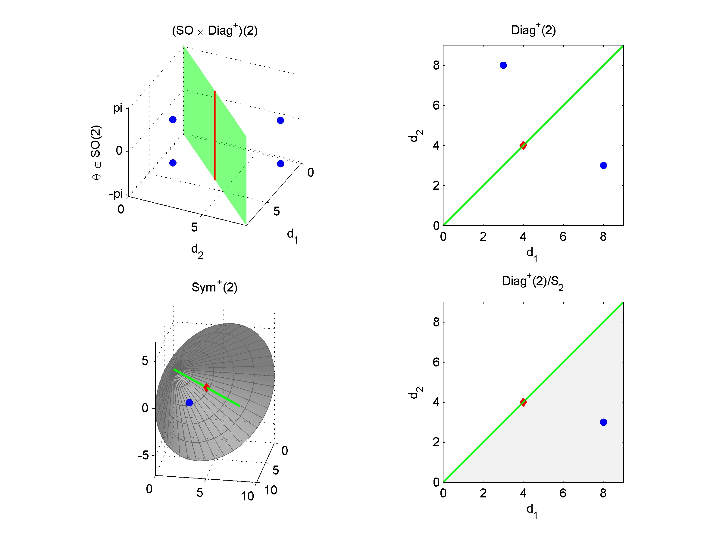
Figure 2: Stratification of $M=SO(2)\times\mbox{Diag}^{+}(2)$ (top left), $\mbox{Sym}^{+}(2)$ (bottom left), $\mbox{Diag}^{+}(2)$ (top right) and $\mbox{Diag}^{+}(2)/S_{2}$ (shaded area in bottom right). ${\rm Sym}^{+}(2)$ is embedded in ${\rm Sym}(2)\cong{\bf R}^{3}$ as the cone $\{(a_{11},a_{22},\sqrt{2}a_{12}):a_{11}>0,a_{22}>0,a_{11}a_{22}-a_{12}^{2}>0\}$. The space ${\rm Diag}^{+}(2)/S_{2}$ is represented as a fundamental domain for the action of $S_{2}$ on ${\rm Diag}^{+}(2)$ (a subset $A\subset{\rm Diag}^{+}(2)$ containing exactly one point of each orbit, and such that ${\rm quo}_{1}:{\rm Diag}^{+}(2)\to{\rm Diag}^{+}(2)/S_{2}$ restricts to a homeomorphism ${\rm quo}_{1}^{-1}(A\setminus\partial A)\to A\setminus\partial A$). Also shown are $X=\mbox{diag}(8,3)\in{\cal S}_{[{\sf J}_{\rm top}]}\subset\mbox{Sym}^{+}(2)$ (blue dot) and $Y={\rm diag}(4,4)\in{\cal S}_{[{\sf J}_{\rm bot}]}$ (red dot), as well as their pre-images in $M$. The projections to ${\rm Diag}^{+}(2)$ and ${\rm Diag}^{+}(2)/S_{2}$ of these subsets of $M$ and ${\rm Sym}^{+}(2)$ are illustrated as correspondingly-colored dots in the right-hand panels.

2.8.2 Example: ${\rm Sym}^{+}(3)$

Stratification of $M$ and ${\rm Diag}^{+}(3)$. There are six strata of $M=(SO\times{\rm Diag}^{+})(3)$ (and of ${\rm Diag}^{+}(3)$), labeled by the six partitions of $\{1,2,3\}$; see Table 2. The features of the stratum ${\cal D}_{{\sf J}}$ we discuss below apply also to the corresponding stratum ${\cal S}_{{\sf J}}=SO(3)\times{\cal D}_{{\sf J}}$.

• The stratum ${\cal D}_{{\sf J}_{\rm bot}}$ is the connected component $\{\mbox{Diag}(d_{1},d_{2},d_{3}):d_{1}=d_{2}=d_{3}\}$. In the top panel of Fig. 3, ${\cal D}_{{\sf J}_{\rm bot}}$ corresponds to the green line.

• The stratum ${\cal D}_{{\sf J}_{1}}$ consists of two connected components: ${\cal D}_{{\sf J}_{1}}^{\rm pro}=\linebreak\{\mbox{Diag}(d_{1},d_{2},d_{3}):d_{1}>d_{2}=d_{3}\}$ and ${\cal D}_{{\sf J}_{1}}^{\rm ob}=\{\mbox{Diag}(d_{1},d_{2},d_{3}):d_{1}<d_{2}=d_{3}\}$. (The superscripts “pro” and “ob” stand for “prolate” and “oblate”, respectively; see below.) The closures of these two connected components intersect in ${\cal D}_{{\sf J}_{\rm bot}}$. In Fig. 3, ${\cal D}_{{\sf J}_{1}}$ corresponds to one of the three shaded planes except the green line. The stratum ${\cal S}_{{\sf J}_{1}}$ also consists of two connected components: ${\cal S}_{{\sf J}_{1}}^{\rm pro}=SO(3)\times{\cal D}_{{\sf J}_{1}}^{\rm pro}$ and ${\cal S}_{{\sf J}_{1}}^{\rm ob}=SO(3)\times{\cal D}_{{\sf J}_{1}}^{\rm ob}$. The strata ${\cal D}_{{\sf J}_{i}}$ and ${\cal S}_{{\sf J}_{i}}$ for $i=2$ and $3$ are similarly characterized.

• The stratum ${\cal D}_{{\sf J}_{\rm top}}$ consists of six connected components, which can be labeled by permutations of $\{1,2,3\}$. Precisely, ${\cal D}_{{\sf J}_{\rm top}}=\bigcup_{\pi\in S_{3}}{\cal D}_{{\sf J}_{\rm top}}^{\pi}$, where ${\cal D}_{{\sf J}_{\rm top}}^{\pi}=\{\mbox{Diag}(d_{1},d_{2},d_{3}):d_{\pi^{-1}(1)}>d_{\pi^{-1}(2)}>d_{\pi^{-1}(3)}\}$ for $\pi\in S_{3}$.

Stratification of ${\rm Sym}^{+}(3)$ and ${\rm Diag}^{+}(3)/S_{3}$. There are three strata of ${\rm Sym}^{+}(3)$ (and of ${\rm Diag}^{+}(3)/S_{3}$), corresponding to the three partitions of 3: $[{\sf J}_{\rm top}]=1+1+1,[{\sf J}_{\rm mid}]=2+1,$ and $[{\sf J}_{\rm bot}]=3$. These stratifications are closely related to an ellipsoid classification. An SPD matrix $X\in{\rm Sym}^{+}(3)$ with eigenvalues $a\geq b\geq c$ corresponds to the ellipsoid given by the equation $x^{T}X^{-1}x=1$, and has the shape of a sphere if $a=b=c$, an oblate spheroid if $a=b>c$, a prolate spheroid if $a>b=c$, or a tri-axial ellipsoid if $a>b>c$. We will say that $X\in{\rm Sym}^{+}(3)$ is prolate (respectively oblate, triaxial) if the corresponding ellipsoid is a prolate spheroid (resp. oblate spheroid, triaxial ellipsoid).

• The stratum ${\cal S}_{[{\sf J}_{\rm top}]}={\cal S}_{1+1+1}$ the set of all SPD matrices with three distinct eigenvalues. Every $X\in{\cal S}_{[{\sf J}_{\rm top}]}$ is tri-axial. In the bottom panel of Fig. 3, the corresponding stratum ${\cal D}_{[{\sf J}_{\rm top}]}\subset{\rm Diag}^{+}(3)$ is depicted as an open convex cone. ${\cal S}_{[{\sf J}_{\rm top}]}$ is connected.

• The stratum ${\cal S}_{[{\sf J}_{\rm mid}]}={\cal S}_{2+1}$ consists of SPD matrices with just two distinct eigenvalues, and is a disjoint union of two connected components: ${\cal S}_{2+1}^{\rm pro}=F({\cal S}_{{\sf J}_{1}}^{\rm pro})$ and ${\cal S}_{2+1}^{\rm ob}=F({\cal S}_{{\sf J}_{1}}^{\rm ob})$. If $X\in{\cal S}_{2+1}^{\rm pro}$, then $X$ is prolate; if $X\in{\cal S}_{2+1}^{\rm ob}$, then $X$ is oblate. Likewise, the stratum ${\cal D}_{2+1}$ is a disjoint union of two connected components: ${\cal D}_{2+1}^{\rm ob}$ and ${\cal D}_{2+1}^{\rm pro}$. In the bottom left panel of Figure 3, the two gray open planar sectors represent these two connected components of ${\cal D}_{2+1}$.

• The stratum ${\cal S}_{[{\sf J}_{\rm bot}]}={\cal S}_{3}$ is the set of all SPD matrices with only one distinct eigenvalue. The corresponding ellipsoids have the shape of a sphere. ${\cal S}_{[{\sf J}_{\rm bot}]}$ is connected.

Fibers of $X\in{\rm Sym}^{+}(3)$.

• For any $X\in{\cal S}_{[{\sf J}_{\rm top}]}={\cal S}_{1+1+1}$, the fiber ${\cal E}_{X}\subset M$ consists of 24 points, all of which lie in ${\cal S}_{{\sf J}_{\rm top}}\in M$.

• For any $X\in{\cal S}_{[{\sf J}_{\rm mid}]}={\cal S}_{2+1}$, the fiber ${\cal E}_{X}\subset M$ is diffeomorphic to 6 copies of the circle.

• For any $X\in{\cal S}_{[{\sf J}_{\rm bot}]}={\cal S}_{3}$, the fiber ${\cal E}_{X}\subset{\cal S}_{{\sf J}_{\rm bot}}\subset M$ is diffeomorphic to (one copy of) $SO(3)$ (and thus to ${\bf R}P^{3}$).

In Figure 3, examples of the three types of fibers are provided. To help visualize, we show the projected fibers, $\mbox{Proj}_{2}({\cal E}_{X})\subset{\rm Diag}^{+}(3)$. (For any $X\in{\cal S}_{k_{1}+\cdots+k_{r}}\subset{\rm Sym}^{+}(p)$, $\mbox{Proj}_{2}({\cal E}_{X})$ is a discrete set of cardinality $\frac{p!}{k_{1}!k_{2}!\ldots k_{r}!}$.)

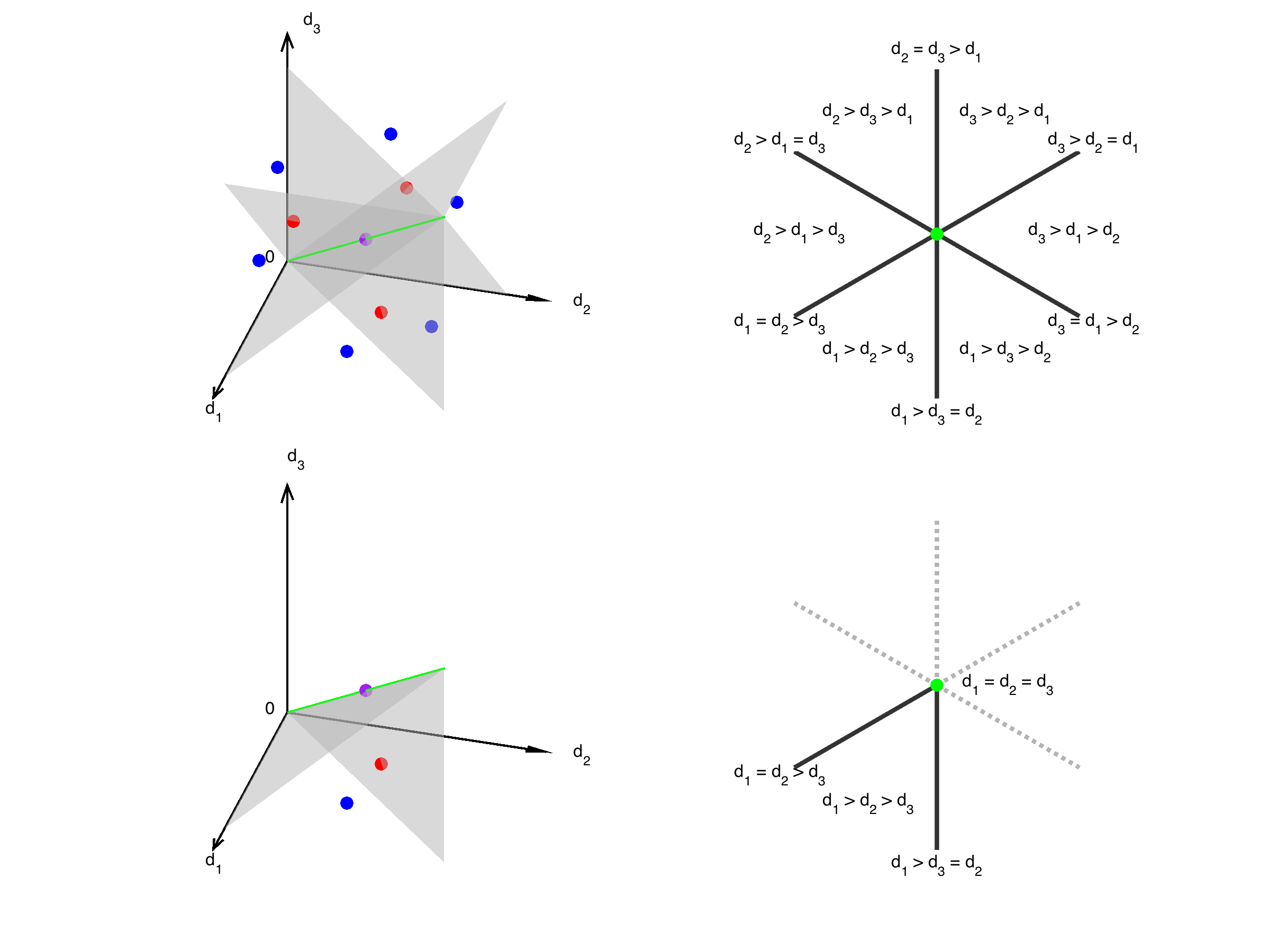
Figure 3: Stratification of ${\rm Diag}^{+}(3)$ (top left) and $\mbox{Diag}^{+}(3)/S_{3}$ (bottom left). The star-figure (top right) represents the intersection of the top left figure and a hyperplane orthogonal to the green line. In the bottom left panel, the space ${\rm Diag}^{+}(3)/S_{3}$ is represented as a fundamental domain for the action of $S_{3}$ on ${\rm Diag}^{+}(3)$, a convex cone bounded by below by the positive quadrant of the $d_{1}d_{2}$-plane and on the sides by the two indicated gray planar sectors. Since the spaces ${\rm Sym}^{+}(3)$ and $M=(SO\times{\rm Diag}^{+})(3)$ are six-dimensional, there are no simple visualizations of them. Also shown are projections of $X=\mbox{diag}(8,5,1)\in{\cal S}_{[{{\sf J}_{\rm top}}]}\subset{\rm Sym}^{+}(3)$ (blue dot), $Y=\mbox{diag}(6,6,2)\in{\cal S}_{{\sf J}_{\rm mid}}$ (red dot), and $Z=\mbox{diag}(5,5,5)\in{\cal S}_{[{{\sf J}_{\rm bot}}]}$ (green dot) to ${\rm Diag}^{+}(3)/S_{3}$ (bottom) and the pre-images of the quotient map in ${\rm Diag}^{+}(3)$ (top).

3 Scaling-rotation framework for curves and distances on $\mbox{Sym}^{+}(p)$

3.1 Smooth scaling-rotation curves

The space of eigen-decompositions $M=SO(p)\times{\rm Diag}^{+}(p)$ is a Riemannian manifold. We define the Riemannian metric $g_{M}$ as a product Riemannian metric determined by metrics on $SO(p)$ and ${\rm Diag}^{+}$ as follows.

The Lie algebra ${\mathfrak{so}}(p)=T_{I}(SO(p))$ is the space of $p\times p$ antisymmetric matrices. In this paper, for $U\in SO(p)$ we identify the tangent space $T_{U}(SO(p))$ with the right-translate of ${\mathfrak{so}}(p)$ by $U$:

$$T_{U}(SO(p))=\{AU:A\in{\mathfrak{so}}(p)\}.$$ (3.1)

The space ${\rm Diag}^{+}(p)$ is also a Lie group, but since it is an open subset of a vector space, namely ${\rm Diag}(p)$, we make the identification $T_{D}({\rm Diag}^{+}(p))={\rm Diag}(p)$ for all $D\in{\rm Diag}^{+}(p)$. The tangent space of $M$ at $(U,D)\in M$ is

$$T_{(U,D)}M=T_{U}(SO(p))\oplus T_{D}({\rm Diag}^{+}(p)).$$

Using (3.1), the standard bi-invariant Riemannian metric $g_{SO}$ on $SO(p)$ is defined by

$$\left.g_{SO}\right|_{U}(A_{1},A_{2})=-\frac{1}{2}\mbox{trace}(A_{1}U^{-1}A_{2}U^{-1}),$$ (3.2)

where $U\in SO(p)$ and $A_{1},A_{2}\in T_{U}(SO(p)).$ A (bi-)invariant Riemannian metric ${g_{{\cal D}^{+}}}$ is defined by setting

$$\left.{g_{{\cal D}^{+}}}\right|_{D}(L_{1},L_{2})=\mbox{trace}(D^{-1}L_{1}D^{-1}L_{2})$$ (3.3)

for $D\in{\rm Diag}^{+}(p)$ and $L_{1},L_{2}\in T_{D}({\rm Diag}^{+}(p)).$ Up to a constant factor, ${g_{{\cal D}^{+}}}$ is the only bi-invariant Riemannian metric on ${\rm Diag}^{+}(p)$ that is also invariant under the action of the symmetric group $S_{p}$. The product Riemannian metric is determined by the metrics above. Specifically, for $(U,D)\in M$ and $(A_{i},L_{i})\in T_{(U,D)}M$ we set

$$\left.g_{M}\right|_{(U,D)}((A_{1},L_{1}),(A_{2},L_{2}))=k\left.g_{SO}\right|_{U}(A_{1},A_{2})+\left.{g_{{\cal D}^{+}}}\right|_{D}(L_{1},L_{2}),$$ (3.4)

where $k>0$ is an arbitrary parameter that can be adjusted as desired for applications. Since the metrics $g_{SO}$ and ${g_{{\cal D}^{+}}}$ are bi-invariant, the geodesics in $M$ can be obtained as either left-translates or right-translates of geodesics through the identity $(I,I)$. In this paper, the right-translates are more convenient, which is why we have chosen the identification (3.1) of the tangent spaces of $SO(p)$.

Definition 1.

A smooth scaling-rotation (SSR) curve is a curve $\chi$ in ${\rm Sym}^{+}(p)$ of the form $F\circ\gamma$, where $\gamma:I\to M$ is a geodesic defined on some interval $I$.

Notation 3.1

For $(U,D)\in M$, $A\in{\mathfrak{so}}(p)$, and $L\in{\rm Diag}(p)$, we define $\gamma_{U,D,A,L}:{\bf R}\to M$ and $\chi_{U,D,A,L}:{\bf R}\to{\rm Sym}^{+}(p)$ by

$$\gamma_{U,D,A,L}(t)=(\exp(tA)U,\exp(tL)D)$$ (3.5)

and

$$\chi_{U,D,A,L}=F\circ\gamma_{U,D,A,L}.$$ (3.6)

We use the same notation $\gamma_{U,D,A,L},$ $\chi_{U,D,A,L}$ for the restrictions of the curves above to any interval.

The curve $\gamma_{U,D,A,L}:{\bf R}\to M$ is the geodesic in $M$ with initial conditions $\gamma(0)=(U,D)$, $\gamma^{\prime}(0)=(AU,DL)\in T_{(U,D)}M$. The curve $\chi_{U,D,A,L}$ in $\mbox{Sym}^{+}(p)$, is the corresponding SSR curve.

3.2 Scaling-rotation distance and MSSR curves

Recall that in any group $G$, an element $g$ is called an involution if $g^{2}$ is the identity element $e$ but $g\neq e$. Thus $R\in SO(p)$ is an involution if $R^{2}=I\neq R$. That is, involutions in $SO(p)$ are reflections. The cut-locus of the identity in $SO(p)$ is precisely the set of all involutions. For every non-involution $R\in SO(p)$, there is a unique $A\in{\mathfrak{so}}(p)$ of smallest norm such that $\exp(A)=R$; we define $\log(R)=A$. If $R$ is an involution, there is more than one smallest-norm $A\in{\mathfrak{so}}(p)$ such that $\exp(A)=R$, and we allow $\log(R)$ to denote the set of all such $A$’s. However, all elements $A$ in this set have the same norm, which we write as $\|\log(R)\|$, where $\|\ \|$ denotes the Frobenius norm on matrices: $\|A\|^{2}=\|A\|_{F}^{2}=\mbox{trace}(A^{T}A)$. Thus $\|\log(R)\|$ is a well-defined real number for all $R\in SO(p)$, even when $\log(R)$ is not a unique element of ${\mathfrak{so}}(p)$. The geodesic-distance function $d_{M}$ on $M$ is then

$$d_{M}^{2}\left((U,D),(V,\Lambda)\right) = k\,d_{SO}(U,V)^{2}+d_{{\cal D}^{+}}(D,\Lambda)^{2}$$

$$= \frac{k}{2}\left\|\log(U^{-1}V)\right\|^{2}+\left\|\log(D^{-1}{\Lambda})\right\|^{2}.$$

Definition 2 ([25, Definition 3.10]).

For $X,Y\in{\rm Sym}^{+}(p)$, the scaling-rotation distance $d_{\cal SR}(X,Y)$ between $X$ and $Y$ is defined by

$$d_{\cal SR}(X,Y):=\inf_{\begin{subarray}{c}(U,D)\in{\cal E}_{X},\\ (V,\Lambda)\in{\cal E}_{Y}\end{subarray}}d_{M}((U,D),(V,{\Lambda})).$$ (3.8)

In [25], $d_{\cal SR}(X,Y)$ is interpreted as “the minimum amount of rotation and scaling needed to deform $X$ into $Y$.” In the following, we provide an equivalent definition of $d_{\cal SR}(X,Y)$ as the minimum length of SSR curves from $X$ to $Y$. However, we have not defined a Riemannian metric on ${\rm Sym}^{+}(p)$, so there is no “automatic” meaning attached to the phrase length of a smooth curve in ${\rm Sym}^{+}(p)$.

Definition 3.

Let $\gamma$ be a piecewise-smooth curve in $M$ and let $\ell(\gamma)$ denote the length of $\gamma$.

• For $X,Y\in{\rm Sym}^{+}(p)$, $\gamma:[0,1]\to M$ is called an $({\cal E}_{X},{\cal E}_{Y})$-minimal geodesic if $\gamma(0)\in{\cal E}_{X},\gamma(1)\in{\cal E}_{Y}$, and $\ell(\gamma)=d_{\cal SR}(X,Y)$.

• A pair of points $((U,D),(V,{\Lambda}))\in{\cal E}_{X}\times{\cal E}_{Y}$ is called a minimal pair if $(U,D)=\gamma(0)$ and $(V,{\Lambda})=\gamma(1)$ for some $({\cal E}_{X},{\cal E}_{Y})$-minimal geodesic $\gamma$.

• A minimal smooth scaling-rotation (MSSR) curve from $X$ to $Y$ is a curve $\chi$ in ${\rm Sym}^{+}(p)$ of the form $F\circ\gamma$ where $\gamma$ is an $({\cal E}_{X},{\cal E}_{Y})$-minimal geodesic. We say that the MSSR curve $\chi=F\circ\gamma$ corresponds to the minimal pair formed by the endpoints of $\gamma$.

• The set of (not necessarily unique) MSSR curves from $X$ to $Y$ is denoted by ${\cal M}(X,Y)$.

• For an SSR curve $\chi$ in ${\rm Sym}^{+}(p)$ we define the length of $\chi$ to be $\ell(\chi):=\inf\{\ell(\gamma):\gamma\ \mbox{is a geodesic in $M$ and}\ F\circ\gamma=\chi\}$.

Definition 3(i) also suggests the obvious fact that an $({\cal E}_{X},{\cal E}_{Y})$-minimal geodesic is a minimal geodesic in the usual sense: it is a curve of shortest length among all piecewise-smooth curves with the same endpoints. From the general theory of geodesics (see e.g. [24]), any such curve $\gamma$ is actually smooth, and, when parametrized at constant speed, satisfies the geodesic equation $\nabla_{\gamma^{\prime}}\gamma^{\prime}\equiv 0$. Thus (3.8) is equivalent to

$$d_{\cal SR}(X,Y)=\inf\left\{\ell(\gamma)\mid\gamma:[0,1]\to M\ \mbox{is a geodesic with}\ \gamma(0)\in{\cal E}_{X}\ ,\ \gamma(1)\in{\cal E}_{Y}\right\}.$$ (3.9)

Now with Definition 3(v), (3.9) becomes

$$d_{\cal SR}(X,Y) = \inf\left\{\ell(\chi)\mid\chi:[0,1]\to{\rm Sym}^{+}(p)\ \mbox{is an SSR curve with}\right.$$ (3.10)

$$\left.\phantom{\inf\left\{\ell(\chi)\mid\right.}\ \chi(0)=X,\,\chi(1)=Y\right\}.$$

Remark 3.2.

As noted in [25], the “scaling-rotation distance” $d_{\cal SR}$ is not a metric on ${\rm Sym}^{+}(p)$; it does not satisfy the triangle inequality. (However, its restriction to the top stratum of ${\rm Sym}^{+}(p)$ is a metric; see [25, Theorem 3.12].)

Computing $d_{\cal SR}(X,Y)$ amounts to optimizing over the fibers of $X$ and $Y$. Choosing $(U,D)\in{\cal E}_{X},(V,{\Lambda})\in{\cal E}_{Y}$, it first appears from (2.17) that this requires optimizing over $(G_{D}^{0}\times{\tilde{S}}_{p}^{+})\times(G_{\Lambda}^{0}\times{\tilde{S}}_{p}^{+})$, thus a “continuous” optimization over $G_{D}^{0}\times G_{\Lambda}^{0}$ for each of the $|{\tilde{S}}_{p}^{+}|^{2}$ elements of ${\tilde{S}}_{p}^{+}\times{\tilde{S}}_{p}^{+}$. However, there is quite a bit of redundancy; clearly it suffices to do a continuous optimization over each pair of connected components (an element of ${\rm Comp}({\cal E}_{X})\times{\rm Comp}({\cal E}_{Y})$) and then a combinatorial optimization over the finite set ${\rm Comp}({\cal E}_{X})\times{\rm Comp}({\cal E}_{Y})$. When both $X$ and $Y$ are in the top stratum, the optimization (3.8) is purely combinatorial. More generally, Proposition 2.14(i) implies that $|{\rm Comp}({\cal E}_{X})|=|{\tilde{S}}_{p}^{+}/\Gamma^{0}_{J_{D}}|=|{\tilde{S}}_{p}^{+}|/|\Gamma^{0}_{{\sf J}_{D}}|$ and $|{\rm Comp}({\cal E}_{Y})|=|{\tilde{S}}_{p}^{+}/\Gamma^{0}_{J_{\Lambda}}|=|{\tilde{S}}_{p}^{+}|/|\Gamma^{0}_{J_{\Lambda}}|$, so the product of these two numbers is an upper bound on the number of continuous optimizations needed. Even this bound is quite crude: using invariances of the metric on $M$, it is not hard to understand that the number of continuous optimizations needed should not exceed $\min\{|{\rm Comp}({\cal E}_{X})|,|{\rm Comp}({\cal E}_{Y})|\}$. (In [25], this idea is used in Theorems 4.2 and 4.3.) However, Proposition 4 below reduces this number further when neither $X$ nor $Y$ lies in the top or bottom stratum. To state the proposition, first recall that given any group $G$ and subgroups $H_{1},H_{2}$, an $(H_{1},H_{2})$ double-coset is an equivalence class under the equivalence relation $\sim$ on $G$ defined by declaring $g_{1}\sim g_{2}$ if there exist $h_{1}\in H_{1},h_{2}\in H_{2}$ such that $g_{2}=h_{1}g_{1}h_{2}$. The set of equivalence classes under this relation is denoted $H_{1}\backslash G/H_{2}$. By a set of representatives of $H_{1}\backslash G/H_{2}$ we mean a subset of $G$ consisting of exactly one element from each $(H_{1},H_{2})$ double-coset.

Proposition 4 ([20, Proposition 4.10]).

Let $X,Y\in{\rm Sym}^{+}(p)$ and let $(U,D)\in{\cal E}_{X},(V,{\Lambda})\in{\cal E}_{Y}$. Let $Z$ be any set of representatives of $\Gamma_{{\sf J}_{D}}^{0}\backslash{\tilde{S}}_{p}^{+}/\Gamma_{{\sf J}_{\Lambda}}^{0}$. Then the scaling-rotation distance from $X$ to $Y$ is given by where

$$\wideparen{d}(g;(U,D),(V,\Lambda))=\min_{R_{U}\in G_{D}^{0},R_{V}\in G_{\Lambda}^{0}}\left\{d_{SO}(UR_{U},VR_{V}P_{g}^{-1})\right\}.$$ (3.11)

Every minimal smooth scaling-rotation curve from $X$ to $Y$ corresponds to some minimal pair whose first element lies in the connected component $[(U,D)]$ of ${\cal E}_{X}$.

To illustrate the reduction in the number of required continuous optimizations (3.11) is reduced in the computation of $d_{\cal SR}(X,Y)$, take for example $p=3$ and $X,Y\in{\cal S}_{[{\sf J}_{\rm mid}]},$ the middle stratum of $\mbox{Sym}^{+}(3)$, defined in Section 2.8.2. In this case we have $|{\rm Comp}({\cal E}_{X})|=|{\rm Comp}({\cal E}_{Y})|=6$, but, as we shall see in Section 5.2.1, the set $Z$ in (LABEL:fibdist8a) has cardinality 3. Thus Proposition 4 reduces the number of continuous optimizations needed down to 3.

3.3 Existence and uniqueness of MSSR curves

From Proposition 2.14, every fiber of $F$ is compact, so the infimum in (3.8) is always achieved. Hence for all $X,Y\in{\rm Sym}^{+}(p)$, there always exists an $({\cal E}_{X},{\cal E}_{Y})$-minimal geodesic, a minimal pair in ${\cal E}_{X}\times{\cal E}_{Y}$, and an MSSR curve from $X$ to $Y$.

Such an MSSR curve may not be unique. In [25], a sufficient condition for uniqueness is given, and an example for $p=2$ is provided. With statistical analysis in mind, it is natural to ask: For which $X$ and $Y$ is there a unique MSSR curve from $X$ to $Y$? We address this question more generally by characterizing ${\cal M}(X,Y)$ for all $X,Y\in{\rm Sym}^{+}(p)$. In Sections 4, 6 and 7, we do this explicitly for low-dimensional cases: $p=2$ and $3$. As preparation for this work, we briefly discuss here how non-uniqueness can occur and introduce a tool used to characterize ${\cal M}(X,Y)$ in low dimensions. A general treatment of this topic can be found in [20].

Different $({\cal E}_{X},{\cal E}_{Y})$-minimal geodesics may or may not project to the same MSSR curve. For given $X,Y$, for uniqueness of an MSSR curve from $X$ to $Y$ to fail, there must be distinct $({\cal E}_{X},{\cal E}_{Y})$-minimal geodesics $\gamma_{i}:[0,1]\to M$, whose endpoints are minimal pairs $((U_{i},D_{i}),(V_{i},{\Lambda}_{i}))\in{\cal E}_{X}\times{\cal E}_{Y},$ $i=1,2$, such that $F\circ\gamma_{1}\neq F\circ\gamma_{2}$. There are two possible ways in which this failure can occur: There exist such $\gamma_{i}$ whose endpoints are distinct minimal pairs $((U_{i},D_{i}),(V_{i},{\Lambda}_{i}))$ (“Type I non-uniqueness”), or the same minimal pair $((U,D),(V,{\Lambda}))$ (“Type II non-uniqueness”).

Since for any $D,{\Lambda}\in{\rm Diag}^{+}(p)$ the minimal geodesic from $D$ to ${\Lambda}$ is unique, Type II non-uniqueness with minimal pair $((U,D),(V,{\Lambda}))$ is equivalent to the existence of two or more minimal geodesics from $U$ to $V$, which is equivalent to $U^{-1}V$ being an involution. For $p=2,3$ it is shown in [25] that Type II non-uniqueness never occurs. This is because that, for $p\leq 3$, for any pair $U,V\in SO(p)$ such that $U^{-1}V$ is an involution, there exists a ${\mbox{\boldmath$\sigma$ \unboldmath}\mbox{}}\in{\cal I}_{p}^{+}$ such that $d_{SO}(UI_{\mbox{\scriptsize\boldmath$\sigma$ \unboldmath}\mbox{}},V)<d_{SO}(U,V)$. In [20], it is further shown that for small enough values of $p$, Type II non-uniqueness never occurs; for large enough $p$, it always occurs. In particular, for $p\leq 4$, for all $X,Y\in{\rm Sym}^{+}(p)$ for which ${\cal M}(X,Y)>1$, the non-uniqueness is purely of Type I.

Our strategy for understanding ${\cal M}(X,Y)$ for $p=2,3$ and all $X,Y\in{\rm Sym}^{+}(p)$ is to list all MSSR curves from $X$ to $Y$. Proposition 4 assures us that, for any $(U,D)\in{\cal E}_{X}$, every MSSR curve from $X$ to $Y$ corresponds to some minimal pair whose first element lies in the connected component $[(U,D)]$ of ${\cal E}_{X}$. We need a way to tell whether MSSR curves corresponding to two minimal pairs with first point in $[(U,D)]$ are the same. The following proposition, a special case of Proposition 4.19 of [20], provides such a tool. We apply this result to the $p=3$ case in Section 6.

Proposition 5.

Let $p\leq 4$, $X,Y\in{\rm Sym}^{+}(p),X\neq Y$. For $i=1,2$ assume that $\chi_{i}=F\circ\gamma_{i}$ is an MSSR curve from $X$ to $Y$ corresponding to the minimal pair $((UR_{U,i},D),(VR_{V,i}\,P_{g_{i}}^{-1},{\Lambda}_{i})),$ where $R_{U,i}\in G_{D}^{0},R_{V,i}\in G_{\Lambda}^{0}$, $g_{i}\in{\tilde{S}}_{p}^{+}$, ${\Lambda}_{i}=\pi_{g_{i}}{\mbox{ \raisebox{-1.084pt}{\bf{\Large$\cdot$}}}}{\Lambda}$, and $\gamma_{i}:[0,1]\to M$ is a geodesic. Then $\chi_{1}=\chi_{2}$ if and only if the following two conditions hold.

• $R_{V,2}P_{g_{2}}^{-1}R_{U,2}^{-1}=R_{V,1}P_{g_{1}}^{-1}R_{U,1}^{-1}\,;$

• There exist $g\in{\tilde{S}}_{p}^{+},R\in G_{D,{\Lambda}_{1}}^{0}$ such that

  $$D = \pi_{g}{\mbox{ \raisebox{-1.084pt}{\bf{\Large$\cdot$}}}}D,$$ (3.12)

  $${\Lambda}_{2} = \pi_{g}{\mbox{ \raisebox{-1.084pt}{\bf{\Large$\cdot$}}}}{\Lambda}_{1},$$ (3.13)

  $$\mbox{\rm and}\ \ \ R_{U,1}^{-1}R_{U,2} = RP_{g}^{-1}\,.$$ (3.14)

4 Scaling–Rotation distance and MSSR curves in $\mbox{Sym}^{+}(2)$

The space $\mbox{Sym}^{+}(2)$ has only two strata: $\mathcal{S}_{\rm bot}:=\mathcal{S}_{[{\sf J}_{\rm bot}]}=\{\lambda I:\lambda>0\}$ and $\mathcal{S}_{\rm top}:=\mathcal{S}_{[{\sf J}_{\rm top}]}=\mbox{Sym}^{+}(2)\backslash\mathcal{S}_{\rm bot}$. To characterize all unique and non-unique cases of minimal smooth scaling-rotation (MSSR) curves in $\mbox{Sym}^{+}(2)$, it suffices to consider two possibilities for the strata in which $X,Y$ lie:

1. $X,Y\in\mathcal{S}_{\rm top}$.

2. $X\in\mathcal{S}_{\rm bot}$ ($Y\in\mathcal{S}_{\rm top}\cup\mathcal{S}_{\rm bot}=\mbox{Sym}^{+}(2)$).

For any $X,Y\in\mbox{Sym}^{+}(2)$, with $a\geq b$, $c\geq d$ and $0\leq\theta<\pi$, one can write

$$X=U\begin{pmatrix}e^{a}&0\\ 0&e^{b}\end{pmatrix}U^{T},\ Y=UR_{\theta}\begin{pmatrix}e^{c}&0\\ 0&e^{d}\end{pmatrix}R_{\theta}^{T}U^{T}$$ (4.1)

where $U\in\mbox{SO}(2)$ and $R_{\theta}=\exp(A_{\theta}),$ $A_{\theta}=\begin{pmatrix}0&-\theta\\ \theta&0\end{pmatrix}$. Denote the apparent eigen-decompositions of $X$ and $Y$ appearing in (4.1) by $(U,D)$ and $(V,\Lambda)$. Then the scaling–rotation curve $\chi$ with parameters $(U,D,A,L)$, where $A=\log(VU^{T})$ and $L=\exp(D^{-1}\Lambda)$, is

$$\chi(t)=(UR_{\theta t})\exp\begin{pmatrix}{(1-t)a+tc}&0\\ 0&{(1-t)b+td}\end{pmatrix}(UR_{\theta t})^{T},$$ (4.2)

satisfying $\chi(0)=X$, $\chi(1)=Y$.

Case (i) ($a>b$, $c>d$). Let $(V_{i},\Lambda_{i}$), $i=1,\ldots,4$ be the four eigen-decompositions of $Y$. Specifically, these four eigen-decompositions are

$$(V_{1},\Lambda_{1}) =(UR_{\theta},\mbox{diag}(e^{c},e^{d})),$$

$$(V_{2},\Lambda_{2}) =(UR_{\theta+\pi},\mbox{diag}(e^{c},e^{d})),$$

$$(V_{3},\Lambda_{3}) =(UR_{\theta+\pi/2},\mbox{diag}(e^{d},e^{c})),$$

$$(V_{4},\Lambda_{4}) =(UR_{\theta-\pi/2},\mbox{diag}(e^{d},e^{c})).$$

Then $d_{\mathcal{S}\mathcal{R}}(X,Y)=\min_{i=1,2,3,4}d_{i}$, where $d_{i}=d((U,D),(V_{i},\Lambda_{i}))$. For $0\leq\theta\leq\pi/2$,

$$d_{1}^{2}=k\theta^{2}+(a-c)^{2}+(b-d)^{2}\leq d_{2}^{2},$$

and equality holds if and only if $\theta=\pi/2$. On the other hand, if $\pi/2<\theta<\pi$,

$$d_{2}^{2}=k(\pi-\theta)^{2}+(a-c)^{2}+(b-d)^{2}<d_{1}^{2},$$

For $0\leq\theta<\pi$,

$$d_{3}^{2}=k(\theta-\pi/2)^{2}+(a-d)^{2}+(b-c)^{2}\leq d_{4}^{2},$$

and equality holds if and only if $\theta=0$. Furthermore, we have

$$d_{1}^{2}<d_{3}^{2}\quad \Longleftrightarrow\quad\theta<\frac{\pi}{4}+\frac{2(a-b)(c-d)}{k\pi},$$

$$d_{2}^{2}<d_{3}^{2}\quad \Longleftrightarrow\quad\theta>\frac{3\pi}{4}-\frac{2(a-b)(c-d)}{k\pi}.$$

These inequalities will be used later in the characterization of all MSSR curves for Case (i).

Case (i) has seven subcases: three in which there is a unique MSSR curve, three in which there are non-unique MSSR curves with multiplicity 2, and one in which there are non-unique MSSR curves with multiplicity 3. We denote these subcases “$d_{i}$”, “$d_{i}=d_{j}$”, and “$d_{1}=d_{2}=d_{3}$” respectively. In the subcase denoted by “$d_{i}$”, the MSSR curve from $X$ to $Y$ is unique, has length $d_{\mathcal{S}\mathcal{R}}(X,Y)=d_{i}$, and corresponds to the minimal pair $((U,D),(V_{i},\Lambda_{i}))$ using (4.2). In the subcase denoted “$d_{i}=d_{j}$”, there are exactly two MSSR curves from $X$ to $Y$, of length $d_{\mathcal{S}\mathcal{R}}(X,Y)=d_{i}=d_{j}$, and corresponding to the minimal pairs $((U,D),(V_{i},\Lambda_{i}))$ and $((U,D),(V_{j},\Lambda_{j}))$. The notation for the last subcase with three MSSR curves is similarly understood.

The seven subcases are distinguished by the relationship of the quantity $m:=\frac{2(a-b)(c-d)}{k\pi}$ and the angle $\theta$. If $m>\min(\theta,\pi-\theta)-\pi/4$, then

$$d_{\mathcal{S}\mathcal{R}}(X,Y)=\left\{\begin{array}[]{ll}d_{1},&\theta<\pi/2,\\ d_{1}=d_{2},&\theta=\pi/2,\\ d_{2},&\theta>\pi/2.\\ \end{array}\right.$$

If $m=\min(\theta,\pi-\theta)-\pi/4$, then

$$d_{\mathcal{S}\mathcal{R}}(X,Y)=\left\{\begin{array}[]{ll}d_{1}=d_{3},&\theta<\pi/2,\\ d_{1}=d_{2}=d_{3},&\theta=\pi/2,\\ d_{2}=d_{3},&\theta>\pi/2.\\ \end{array}\right.$$

Finally, if $m<\min(\theta,\pi-\theta)-\pi/4$, then $d_{\mathcal{S}\mathcal{R}}(X,Y)=d_{3}.$ The conditions leading to these seven subcases are graphically summarized in Fig. 4.

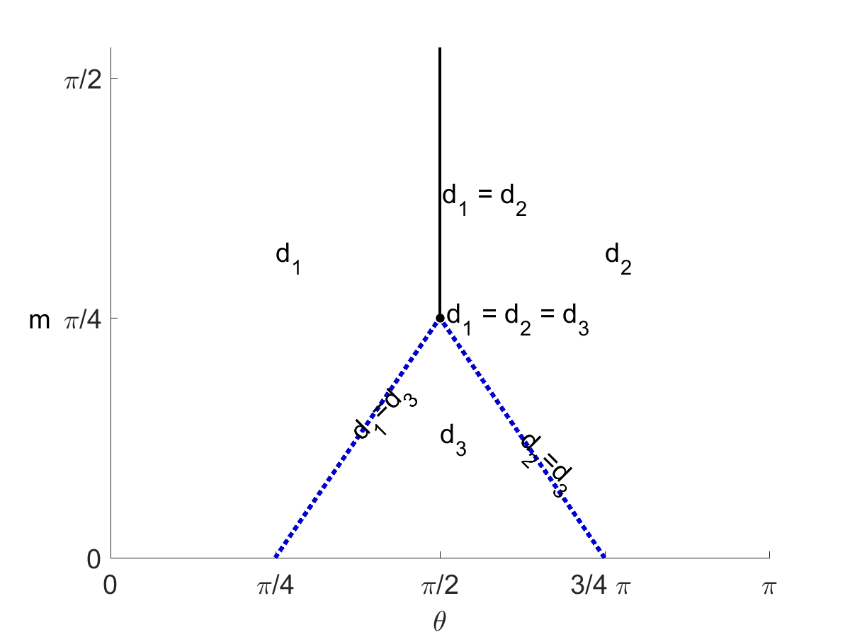
Figure 4: Unique and non-unique MSSR curves in $\mbox{Sym}^{+}(2)$: Schematic illustration for the seven subcases of Case (i) in which both $X$ and $Y$ are in $\mathcal{S}_{\rm top}$.

The MSSR curves corresponding to subcases “$d_{1}$” and “$d_{2}$” can be understood as the rotation and scaling of the ellipse corresponding to $X$ to the ellipse corresponding to $Y$, where the rotation is either counterclockwise (case “$d_{1}$”), or clockwise (case “$d_{2}$”). (There is no rotation in subcase “$d_{1}$” if $\theta=0$.) In these two subcases, the whole MSSR curve never leaves the distinct-eigenvalue subset of $\mbox{Sym}^{+}(2)$ (the top stratum). On the other hand, the MSSR curves corresponding to “$d_{3}$” always pass through the equal-eigenvalue subset of $\mbox{Sym}^{+}(2)$ (the bottom stratum). The direction of rotation for “$d_{3}$” depends on $\theta$: counterclockwise if $\theta<\pi/2$, clockwise if $\theta>\pi/2$. (There is no rotation if $\theta=\pi/2$.)

A few of these seven subcases are illustrated by representative examples in Figs. 5 and 6. If “$d_{1}$” and “$d_{2}$” are thought of as the same “type”, then there are five different types of (non-)uniqueness behavior of MSSR curves in Case (i), as follows:

1. Unique MSSR curve (completely contained in the distinct-eigenvalue subset), if $m>\min(\theta,\pi-\theta)-\pi/4$ and $\theta\neq\pi/2$. Subcases “$d_{1}$” (Fig. 5) and “$d_{2}$” are of this type.

2. Unique MSSR curve (leaving the distinct-eigenvalue subset and passing through the bottom stratum), if $m<\min(\theta,\pi-\theta)-\pi/4$. Subcase “$d_{3}$” is of this type.

3. Two MSSR curves with rotation angle $\pi/2$ (still completely contained in the distinct-eigenvalue subset), if $m>\min(\theta,\pi-\theta)-\pi/4$ and $\theta=\pi/2$. Case “$d_{1}=d_{2}$” is of this type.

4. Two MSSR curves (one in the distinct eigenvalue subset, the other passing through the bottom stratum), if $m=\min(\theta,\pi-\theta)-\pi/4$ and $\theta\neq\pi/2$. Subcases “$d_{1}=d_{3}$” and “$d_{2}=d_{3}$” are of this type.

5. Three MSSR curves (two with rotation-angle $\pi/2$, completely contained in the distinct-eigenvalue subset, and the other involving no rotation but passing through the bottom stratum), if $m=\min(\theta,\pi-\theta)-\pi/4$ and $\theta=\pi/2$. Subcase “$d_{1}=d_{2}=d_{3}$” (Fig. 6) is of this type.

For each given $X$ and $Y$, if one takes $k$ small enough that $m>\pi/4$, then MSSR curves from $X$ to $Y$ are always of type “$d_{1}$” or “$d_{2}$”. In other words, if $k$ is small enough (for fixed $X,Y$), the MSSR curve(s) are completely contained in the distinct-eigenvalue subset.

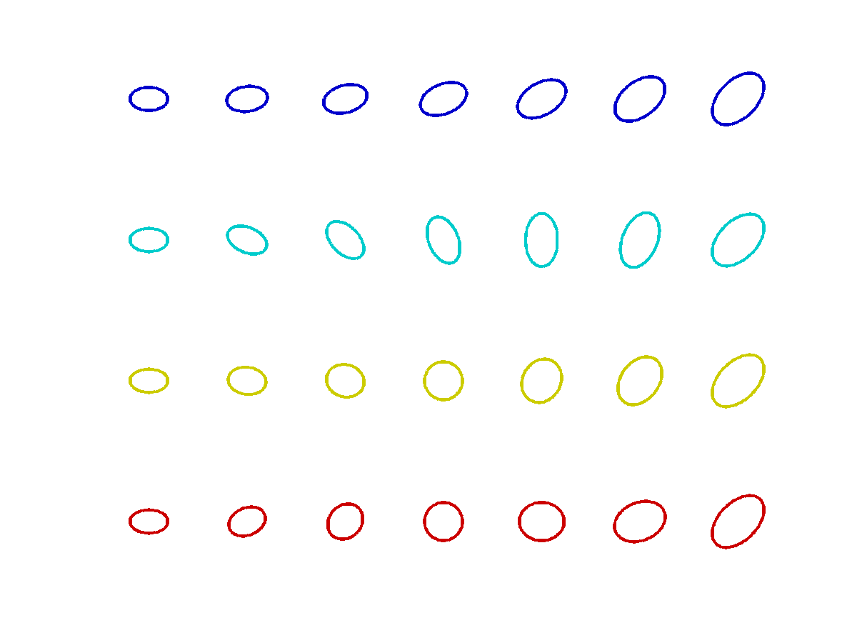
Figure 5: An example for subcase “$d_{1}$”. For each $i=1,2,3,4$, “curve $i$” represents the scaling-rotation curve corresponding to the pair $((U,D),(V_{i},\Lambda_{i}))$, and whose length is $d_{i}$. $\mbox{Sym}^{+}(2)$ is an open cone in the three-dimensional space $\mbox{Sym}(2)$. The black line is the axis of the cone. Each curve, labeled by the same color in the left and right panels, is illustrated as the space curve $\chi(t)$, contained in this cone $\mbox{Sym}^{+}(2)$ (left), or as the sequence of corresponding ellipses (right). In this and all other examples, the scaling factor $k$ is set equal to $1$.

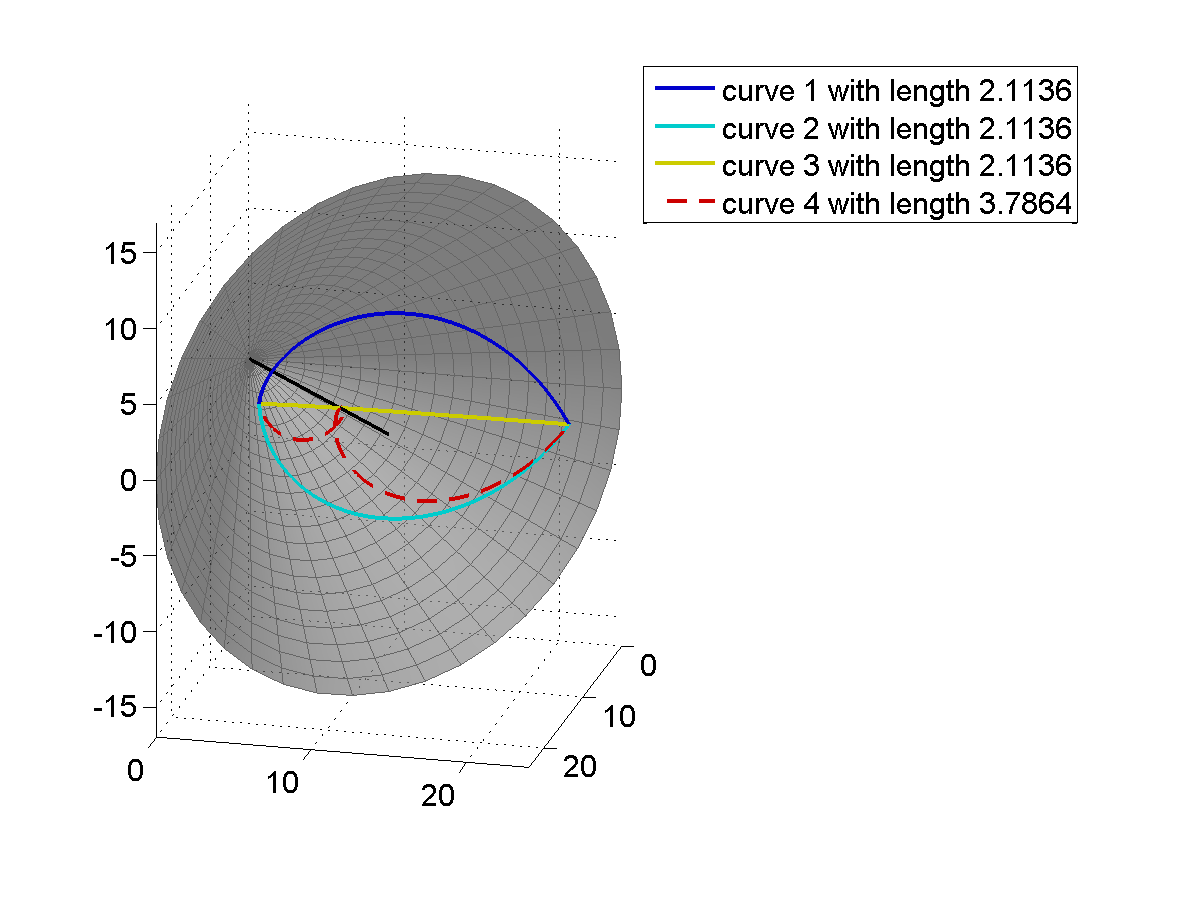
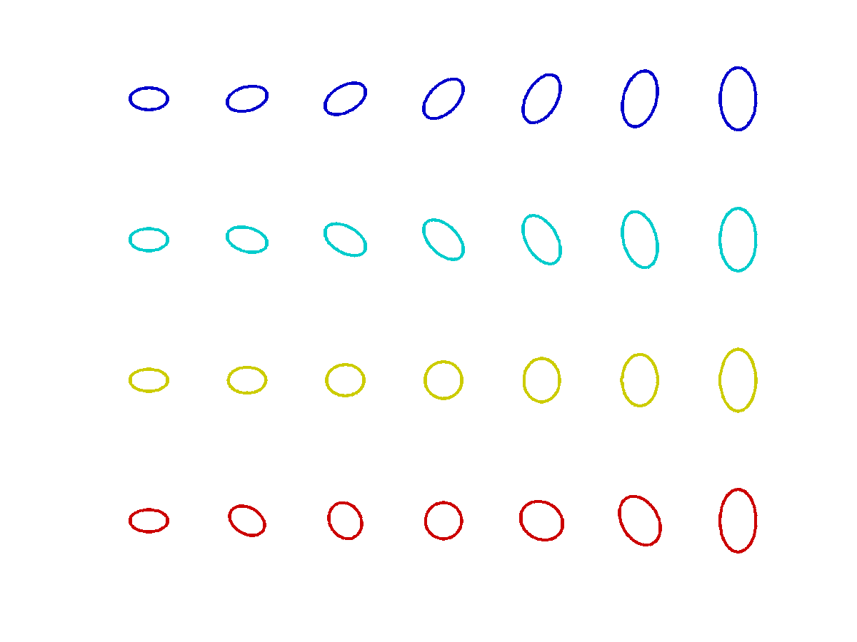
Figure 6: An example for subcase “$d_{1}=d_{2}=d_{3}$”.

Case (ii) ($a=b$ and $c\geq d$). By Theorem 4.1 of [25], the MSSR curve from $X$ to $Y$ is unique, and is

$$\chi(t)=(UR_{\theta})\exp\begin{pmatrix}{(1-t)a+tc}&0\\ 0&{(1-t)a+td}\end{pmatrix}(UR_{\theta})^{T},$$

and $d_{\mathcal{S}\mathcal{R}}(X,Y)=\sqrt{(a-c)^{2}+(a-d)^{2}}$. If in addition $c=d$, then $\chi(t)=e^{(1-t)a+tc}I$.

5 Scaling-rotation distances on ${\rm Sym}^{+}(3)$

For the case $p=3$, we will obtain explicit formulas for all MSSR curves and scaling-rotation distances by using the quaternionic parametrization of $SO(3)$. In Section 6, we use this to give explicit descriptions of the set ${\cal M}(X,Y)$ of MSSR curves between two points $X,Y\in{\rm Sym}^{+}(3)$ in all “nontrivial” cases (as defined later in this section).

5.1 Characterization of SR distance using quaternions

5.1.1 Relation of quaternions to ${\rm SO}(3)$

The space ${\bf H}$ of quaternions, with its usual real basis $\{1,i,j,k\}$ identified with the standard basis of ${\bf R}^{4}$, and with $\{i,j,k\}$ identified with the standard basis of ${\bf R}^{3}$, provides a convenient parametrization of $SO(3)$. Specifically, writing $S^{3}_{\bf H}=$ $\{x_{0}+x_{1}i+x_{2}j+x_{3}k\ :\ x_{0}^{2}+x_{1}^{2}+x_{2}^{2}+x_{3}^{2}=1\}$, there is a natural two-to-one Lie-group homomorphism $\phi:S^{3}_{\bf H}\to SO(3)$, defined as follows. Using the basis $\{i,j,k\}$ to identify ${\bf R}^{3}$ with ${\rm Im({\bf H})}$, the space of purely imaginary quaternions, for $q\in S^{3}_{\bf H}$ and $x\in{\rm Im({\bf H})}$ we set $\phi(q)(x)=qx\bar{q}$, which lies in ${\rm Im({\bf H})}$. For $q_{1},q_{2}\in S^{3}_{\bf H}$ we have $\phi(q_{2})=\phi(q_{1})$ if and only if $q_{2}=\pm q_{1}.$ Thus, for any $U\in SO(3)$, if $q_{U}\in\phi^{-1}(U)$ then

$$\phi^{-1}(U)=\{\pm q_{U}\}.$$ (5.1)

Let $S^{2}_{\rm Im({\bf H})}=\{\tilde{a}\in{\rm Im({\bf H})}\ :\ \|\tilde{a}\|=1\}$. For $\tilde{a}\in S^{2}_{\rm Im({\bf H})}$ and $\theta\in[0,\pi]$ let $R_{\theta,\tilde{a}}$ denotes counterclockwise rotation by angle $\theta$ about the axis $\tilde{a}$ (“counterclockwise” as determined by $\tilde{a}$ using the right-hand rule). Let

$$SO(3)_{<\pi}:=\{R_{\theta,\tilde{a}}\ :\ \tilde{a}\in S^{2}_{\rm Im({\bf H})},\theta\in[0,\pi)\},$$

the set of non-involutions in $SO(3)$. The map $s:SO(3)_{<\pi}\to S^{3}_{\bf H}$ defined by

$$s(R_{\theta,\tilde{a}})=\cos\frac{\theta}{2}+(\sin\frac{\theta}{2})\tilde{a}$$ (5.2)

is a smooth right-inverse to $\phi$ on $SO(3)_{<\pi}$ (i.e., $\phi\circ s$ is the identity map on this domain), but $s$ is not a homomorphism and cannot be extended continuously to all of $SO(3)$.

Distances between elements of $SO(3)$ are related very simply to geodesic distances in $S^{3}_{\bf H}$ with respect to the standard Riemannian metric on $S^{3}=S^{3}_{\bf H}$. For $U,V\in SO(3)$,

$$d_{SO}(U,V) = 2\min\{d_{S^{3}}(r_{U},r_{V})\ :\ r_{U}\in\phi^{-1}(U),r_{V}\in\phi^{-1}(V)\}$$

$$= 2\cos^{-1}|{\rm Re}(\overline{r_{U}}\ r_{V})|\ \mbox{\rm where $r_{U},r_{V}$ are as in previous line.}$$

Alternatively, $d_{SO}(U,V)=d_{SO}(I,U^{-1}V)=2\cos^{-1}|{\rm Re}(q_{U^{-1}V})|$, where $q_{U^{-1}V}$ is either of the two elements of $\phi^{-1}(U^{-1}V)$. Thus

$$d_{SO}(U,V)=2\cos^{-1}|{\rm Re}(\overline{q_{U}}\ q_{V})|=2\cos^{-1}|{\rm Re}(q_{U^{-1}V})|$$ (5.3)

where each of $q_{U},q_{V},q_{U^{-1}V}$ is either of the two elements in $S^{3}$ mapped by $\phi$ to $U,V,$ and $U^{-1}V$ respectively.

5.1.2 Quaternionic pre-images of signed-permutation matrices

For every subgroup $H\subset SO(3)$, let $\widehat{H}$ denote the pre-image $\phi^{-1}(H)\subset S^{3}_{\bf H}$. Writing $\Gamma:={\tilde{S}}_{3}^{+}\subset SO(3)$, the 24-element group of even signed-permutation matrices, the 48 elements of $\widehat{\Gamma}$ are the following:

$$\pm 1,\pm i,\pm j,\pm k,$$ (5.4)

$$\frac{1}{\sqrt{2}}(\pm e_{m}\pm e_{n}),\mbox{where}\ e_{0}=1,e_{2}=i,e_{3}=j,e_{4}=k,\ \mbox{and}\ m<n,$$ (5.5)

$$\frac{1}{2}(\pm 1\pm i\pm j\pm k)$$ (5.6)

(all sign-combinations allowed in all sums). Under $\phi$, the eight elements (5.4) are mapped to the four even sign-change matrices, the 24 elements (5.5) are mapped to the 12 positive-determinant “signed transposition matrices” (permutation-matrices corresponding to transpositions, with an odd number of 1’s replaced by $-1$’s), and the 16 elements (5.6) are mapped to the 8 positive-determinant “signed cyclic-permutation matrices” (permutation matrices corresponding to cyclic permutations, with an even number of 1’s replaced by $-1$’s).

5.1.3 Parameters corresponding to different strata

For any subgroups $H_{1},H_{2}$ of $SO(3)$, the map $\phi$ induces a bijection $\widehat{H_{1}}\backslash\widehat{\Gamma}/\widehat{H_{2}}\to H_{1}\backslash\Gamma/H_{2}$. Thus if $\widehat{Z}$ is a set of representatives of $\widehat{\Gamma_{D}^{0}}\backslash\widehat{\Gamma}/\widehat{\Gamma_{\Lambda}^{0}}$ in $\widehat{\Gamma}$, then $\phi(\widehat{Z})$ is a set $Z$ of representatives of $\Gamma_{D}^{0}\backslash\Gamma/\Gamma_{\Lambda}^{0}$ in $\Gamma$.

Now let $X,Y,(U,D),$ and $(V,{\Lambda})$ be as in Proposition 4, and let $\widehat{Z}$ be a set of representatives of $\widehat{\Gamma_{D}^{0}}\backslash\widehat{\Gamma}/\widehat{\Gamma_{\Lambda}^{0}}$. For $\zeta\in\widehat{\Gamma}$, define $\pi_{\zeta}=\pi_{\phi(\zeta)}\in S_{3}$ (see Notation 2.11).

From equation (5.3) and the fact that $\phi$ is a homomorphism, it follows that in the setting of equation (LABEL:fibdist8a) (with $p=3$), for all $r_{U}\in\phi^{-1}(R_{U}),r_{V}\in\phi^{-1}(R_{V}),g\in{\tilde{S}}_{3}^{+},$ and $\zeta_{g}\in\phi^{-1}(g)$,

$$d_{SO}(UR_{U},VR_{V}P_{g}^{-1})^{2}=4\left(\cos^{-1}\left|{\rm Re}\left(r_{V}\ \overline{\zeta_{g}}\ \overline{r_{U}}\ q_{U^{-1}V}\right)\right|\right)^{2}.$$ (5.7)

From Proposition 4, we therefore have

$$d_{\cal SR}(X,Y)^{2} =\min_{\zeta\in\widehat{Z}}\left\{k\,\hat{d}(\zeta)^{2}+\|\log({\Lambda}_{\pi_{\zeta}}D^{-1})\|^{2}\right\},$$ (5.8)

where

$$\hat{d}(\zeta):=\breve{d}(\zeta;\widehat{G_{D}^{0}},\widehat{G_{\Lambda}^{0}},q_{U^{-1}V}):=\min_{r_{U}\in\widehat{G_{D}^{0}},r_{V}\in\widehat{G_{\Lambda}^{0}}}\left\{\cos^{-1}|{\rm Re}\left(r_{V}\ \bar{\zeta}\ \overline{r_{U}}\ q_{U^{-1}V}\right)|\right\}.$$ (5.9)

As equations (5.8)-(5.9) suggest, computing $d_{\cal SR}(X,Y)$ is a minimization problem that breaks into two parts, one over the discrete parameter-set $\widehat{Z}$ and the other over the (potentially) “continuous” parameter-set $\widehat{G_{D}^{0}}\times\widehat{G_{\Lambda}^{0}}$. Both parameter-sets depend on $X$ and $Y$.

If $X$ or $Y$ lies in the bottom stratum of $\mbox{Sym}^{+}(3)$ (i.e., has only one distinct eigenvalue), then the set $\widehat{Z}$ has only one element $\zeta$, which we can take to be $1\in{\bf H}$, and at least one of the groups $\widehat{G_{D}^{0}},\widehat{G_{\Lambda}^{0}}$ is all of $S^{3}_{\bf H}$. The set $\left\{r_{V}\ \bar{\zeta}\ \overline{r_{U}}:(r_{U},r_{V})\in\widehat{G_{D}^{0}}\times\widehat{G_{\Lambda}^{0}}\right\}$ is simply $S^{3}_{\bf H}$, the inner minimum $\hat{d}(\zeta)$ in (5.8) is 0, and we immediately obtain $d_{\cal SR}(X,Y)=\|\log({\Lambda}D^{-1})\|$. We do not need to use quaternions to obtain this result; it follows just as quickly from (LABEL:fibdist8a).

At the other extreme, if $X$ and $Y$ both lie in the top stratum of ${\rm Sym}^{+}(p)$ (i.e. both have three distinct eigenvalues) then $\widehat{G_{D}^{0}}=\widehat{G_{\Lambda}^{0}}=\{\pm 1\}$, and the inner minimum is trivial to compute ($\hat{d}(\zeta)=\cos^{-1}|{\rm Re}(\bar{\zeta}q_{U^{-1}V})|$), so we are reduced immediately to a single minimization over $\widehat{Z}$. As in the previous case, we do not need the quaternionic reframing of the distance formula at all: already in (LABEL:fibdist8a) we have $G_{D}^{0}=G_{\Lambda}^{0}=\{I\}$, so the distance can be found simply by minimizing over the discrete variable $g\in Z=\tilde{S}_{3}^{+}$. We need only have a computer calculate $d_{M}((U,D),(VP_{g}^{-1},g{\mbox{ \raisebox{-1.084pt}{\bf{\Large$\cdot$}}}}{\Lambda})$ for each of the 24 $g$’s and return the corresponding minimal pairs and MSSR curves. For combinatorial reasons, a complete algebraic classification of the pairs $(X,Y)$ (with $X,Y$ both in the top stratum of ${\rm Sym}^{+}(3)$) for which ${\cal M}(X,Y)$ has a given cardinality would be very complex, and we do not attempt this.

For the above reasons, for the remainder of this section we focus on the cases in which $X$ and $Y$ do not both lie in the top stratum of ${\rm Sym}^{+}(3)$, and neither lies in the bottom stratum. Thus we restrict attention to the cases in which one of the matrices $X,Y$ has exactly two distinct eigenvalues, and the other has either two or three. We refer to these cases as the “nontrivial” cases (because the set of distances between elements of ${\cal E}_{X}$ and elements of ${\cal E}_{Y}$ is not a finite set). To analyze them we introduce the following notation:

$${\cal S}_{\rm top} :={\cal S}_{[{\sf J}_{\rm top}]}={\cal S}_{1+1+1}\subset{\rm Sym}^{+}(3),$$

$${\cal S}_{\rm mid} :={\cal S}_{[{\sf J}_{\rm mid}]}={\cal S}_{2+1}\subset{\rm Sym}^{+}(3),$$

$${\cal D}_{{\sf J}_{1}} :={\cal D}_{\{\{1\},\{2,3\}\}}=\{{\rm diag}(d_{1},d_{2},d_{2}):\ d_{1},d_{2}>0,\ d_{1}\neq d_{2}\}\subset{\rm Diag}^{+}(3).$$

5.2 Scaling-rotation distances for ${\rm Sym}^{+}(3)$ in the nontrivial cases

From now through Section 6 we assume that $X\in{\cal S}_{\rm mid}$ and that either $Y\in{\cal S}_{\rm top}$ or $Y\in{\cal S}_{\rm mid}$. Then $X$ has an eigen-decomposition $(U,D)$ with $D\in{\cal D}_{{\sf J}_{1}}$, and if $Y\in{\cal S}_{\rm mid}$ then $Y$ has a eigen-decomposition $(V,{\Lambda})$ with ${\Lambda}\in{\cal D}_{{\sf J}_{1}}$. We will always assume that our pairs $(U,D),(V,{\Lambda})$ have been chosen this way. Then we have

$$G_{D}^{0}=G_{{\cal D}_{{\sf J}_{1}}}^{0}:=\left\{\left[\begin{array}[]{cl}1&{\bf 0}^{T}\\ {\bf 0}&R\end{array}\right]\ :\ R\in SO(2)\right\},\ \ G_{\Lambda}^{0}=\left\{\begin{array}[]{ll}\{I\}&\mbox{if $Y\in{\cal S}_{\rm top}$,}\\ G_{{\cal D}_{{\sf J}_{1}}}^{0}&\mbox{if $Y\in{\cal S}_{\rm mid}$.}\end{array}\right.$$

It is not hard to check that

$$\widehat{G_{D}^{0}} = S^{1}_{\bf C}:=\{\exp(ti)\ :\ t\in{\bf R}\}\subset{\bf C}\subset{\bf H},$$ (5.10)

$$\widehat{G_{\Lambda}^{0}} = \left\{\begin{array}[]{ll}\{\pm 1\}&\mbox{if $Y\in{\cal S}_{\rm top}$,}\\ S^{1}_{\bf C}&\mbox{if $Y\in{\cal S}_{\rm mid}$.}\end{array}\right.$$ (5.13)

The inner minimum in (5.8) is then

$$\hat{d}(\zeta)=\left\{\begin{array}[]{ll}\min_{r_{U}\in S^{1}_{\bf C}}\left\{\cos^{-1}\left|{\rm Re}\left(\bar{\zeta}\ \overline{r_{U}}\ q_{U^{-1}V}\right)\right|\right\}&\mbox{if $Y\in{\cal S}_{\rm top}$,}\\ \min_{r_{U},r_{V}\in S^{1}_{\bf C}}\left\{\cos^{-1}\left|{\rm Re}\left(r_{V}\ \bar{\zeta}\ \overline{r_{U}}\ q_{U^{-1}V}\right)\right|\right\}&\mbox{if $Y\in{\cal S}_{\rm mid}$.}\end{array}\right.$$ (5.14)

Obviously, minimizing the arc-cosines above is equivalent to maximizing

$$\left|{\rm Re}\left(\bar{\zeta}\ \overline{r_{U}}\ q_{U^{-1}V}\right)\right| Y\in{\cal S}_{\rm top}\,,\phantom{\int_{a}^{b}}$$ if (5.15)

$$\left|{\rm Re}\left(r_{V}\ \bar{\zeta}\ \overline{r_{U}}\ q_{U^{-1}V}\right)\right| Y\in{\cal S}_{\rm mid}\,,$$ if (5.16)

where the maximum is taken over $(r_{U},r_{V})\in S^{1}_{\bf C}\times S^{1}_{\bf C}$ in (5.16), and over just $r_{U}\in S^{1}_{\bf C}$ in (5.15).

5.2.1 The discrete parameter-sets $\widehat{Z}$ in the nontrivial cases

To compute the outer minimum (over $\zeta$) in (5.8), we will need to select sets $\widehat{Z}$ of representatives of $\widehat{\Gamma_{D}^{0}}\backslash\widehat{\Gamma}/\widehat{\Gamma_{\Lambda}^{0}}$ in two cases: (i) ${\sf J}_{D}={\sf J}_{1}:=\{1,\{2,3\}\},{\sf J}_{\Lambda}={{\sf J}_{\rm top}}:=\{\{1\},\{2\},\{3\}\}$, and (ii) ${\sf J}_{D}={\sf J}_{1}={\sf J}_{\Lambda}$. Let us write $\Gamma_{1}:=\Gamma_{{\sf J}_{1}}^{0}$. For case (i), since $\widehat{\Gamma_{{{\sf J}_{\rm top}}}^{0}}=\{\pm 1\}$, which commutes with every element of $\widehat{\Gamma}$ and is a subgroup of $\widehat{\Gamma_{\sf J}^{0}}$ for every ${\sf J}$, the double-coset space $\widehat{\Gamma_{1}}\backslash\widehat{\Gamma}/\widehat{\Gamma_{{{\sf J}_{\rm top}}}^{0}}$ is simply the set $\widehat{\Gamma_{1}}\backslash\widehat{\Gamma}$ of right $\widehat{\Gamma_{1}}$-cosets in $\widehat{\Gamma}$. Observe that $\widehat{\Gamma_{1}}=\widehat{G_{{\sf J}_{1}}^{0}}\ \mbox{\small\ $\bigcap$\ }\ \widehat{\Gamma}=S^{1}_{\bf C}\ \mbox{\small\ $\bigcap$\ }\widehat{\Gamma}=\{\pm 1,\pm i,\frac{\pm 1\pm i}{\sqrt{2}}\}=\{e^{2n\pi i/8}:n=0,1,\dots,7\}$. Thus the cardinality of $\widehat{\Gamma_{1}}\backslash\widehat{\Gamma}$ is 48/8 = 6. One can check that the following set $\widehat{Z}_{1,*}$ contains a representative of each of the six right $\widehat{\Gamma_{1}}$-cosets:

$$\widehat{Z}_{1,*}:=\left\{1,\ j,\frac{1\pm j}{\sqrt{2}},\ \frac{1\pm k}{\sqrt{2}}\right\}.$$ (5.17)

For case (ii), the double-coset space can be viewed as the set of orbits under the action of $\widehat{\Gamma_{1}}$ on $\widehat{\Gamma_{1}}\backslash\widehat{\Gamma}$ (the coset-space in case (i)) by right-multiplication. Thus a set of representatives can be found by imposing the double-coset equivalence relation on the set $\widehat{Z}_{1,*}$ above. The four elements $\frac{1\pm j}{\sqrt{2}},\ \frac{1\pm k}{\sqrt{2}}$ all lie in the same $\widehat{\Gamma_{1}}$ double-coset, since

$$-i\frac{1+j}{\sqrt{2}}i=\frac{1-j}{\sqrt{2}},\ \ -i\frac{1+k}{\sqrt{2}}i=\frac{1-k}{\sqrt{2}},\ {\rm and}\ \frac{1+i}{\sqrt{2}}\,\frac{1+j}{\sqrt{2}}\,\frac{1-i}{\sqrt{2}}=\frac{1+k}{\sqrt{2}}\ .$$

It is easily checked that no two of $1,j$, and $\frac{1+j}{\sqrt{2}}$ lie in the same $(\widehat{\Gamma_{1}},\widehat{\Gamma_{1}})$ double-coset. Hence $Z_{1,1}:=\{1,j,\frac{1+j}{\sqrt{2}}\}$ is a set of representatives of $\widehat{\Gamma_{1}}\backslash\widehat{\Gamma}/\widehat{\Gamma_{1}}$.

The elements $\zeta$ of $Z_{1,*}$ are listed in Table 3, along with the images $\phi(\zeta)\in SO(3)$ and $\pi_{\zeta}\in S_{3}.$ Since $Z_{1,1}\subset Z_{1,*}$, a separate listing for $Z_{1,1}$ is not needed. In Table 3 and henceforth, we write ${\pi_{\rm id}}$ for the identity permutation, and, for distinct $a,b\in\{1,2,3\}$, we write $\pi_{ab}$ for the transposition $(ab)$, the permutation that just interchanges $a$ and $b$.

Table 3: Representatives of the double-coset space $\widehat{\Gamma_{1}}\backslash\widehat{\Gamma}/\widehat{\Gamma_{{{\sf J}_{\rm top}}}^{0}}=\widehat{\Gamma_{1}}\backslash\widehat{\Gamma}$, where $\widehat{\Gamma_{1}}=\widehat{\Gamma_{{\sf J}_{1}}^{0}}$. A set of representatives of $\widehat{\Gamma_{1}}\backslash\widehat{\Gamma}/\widehat{\Gamma_{1}}$ is $\widehat{Z}_{1,1}:=\{1,j,\zeta_{j,+}\}$.

$\zeta\in\widehat{Z}_{1,*}$	1	$j$	$\zeta_{j,\epsilon}:=\frac{1+\epsilon j}{\sqrt{2}}\,,\epsilon\in\{\pm 1\}$	$\zeta_{k,\epsilon}:=\frac{1+\epsilon k}{\sqrt{2}}\,,\epsilon\in\{\pm 1\}$
$\phi(\zeta)\in Z_{1,*}$	$I$	$\left[\begin{array}[]{rrr}-1&0&0\\ 0&1&0\\ 0&0&-1\end{array}\right]$	$\left[\begin{array}[]{rrr}0&0&\epsilon\\ 0&1&0\\ -\epsilon&0&0\end{array}\right]$	$\left[\begin{array}[]{rrr}0&-\epsilon&0\\ \epsilon&0&0\\ 0&0&1\end{array}\right]$
$\pi_{\zeta}\in S_{3}$	${\pi_{\rm id}}$	${\pi_{\rm id}}$	$\pi_{13}$	$\pi_{12}$

Remark 5.1.

As seen in Section 2.8.2, ${\cal E}_{X}$ has six connected components, each diffeomorphic to the circle $G_{{\sf J}_{1}}^{0}$. In Proposition 2.14, for general $p$ and $X$ we exhibited a bijection between ${\rm Comp}({\cal E}_{X})$ and the left-coset space ${\tilde{S}}_{p}^{+}/\Gamma_{{\sf J}_{D}}^{0}$. For any group $G$ and subgroup $H$, the inversion map $G\to G$ induces a 1-1 correspondence between left $H$-cosets and right $H$-cosets, so (for general $p$ and $X$), ${\rm Comp}({\cal E}_{X})$ is also in bijection with $\Gamma_{{\sf J}_{D}}^{0}\backslash{\tilde{S}}_{p}^{+}$. In our current $p=3,X\in{\cal S}_{\rm mid}$ setting, the set $Z_{1,*}:=\{\phi(\zeta)\ :\ \zeta\in\widehat{Z}_{1,*}\}$ is a set of representatives of $\Gamma_{1}\backslash{\tilde{S}}_{3}^{+}/\Gamma_{{{\sf J}_{\rm top}}}=\Gamma_{1}\backslash{\tilde{S}}_{3}^{+}$. The fact that right $\Gamma_{1}$-cosets appear here instead of left cosets is an artifact of our having chosen $X$, rather than $Y$, to lie in ${\cal S}_{\rm mid}$.

5.2.2 Hypercomplex reformulation of the continuous-parameter minimization

We now have

$$d_{\cal SR}(X,Y)^{2}=d_{M}({\cal E}_{X},{\cal E}_{Y})^{2}=$$

$$\left\{\begin{array}[]{l}\displaystyle\min_{\zeta\in\widehat{Z}_{1,*}}\left(4k\left[\min_{r_{U}\in S^{1}_{\bf C}}\left\{\cos^{-1}\left|{\rm Re}\left(\bar{\zeta}\ \overline{r_{U}}\ q_{U^{-1}V}\right)\right|\right\}\right]^{2}+\|\log({\Lambda}_{\pi_{\zeta}}D^{-1})\|^{2}\right)\\ \mbox{\hskip 72.26999pt if $Y\in{\cal S}_{\rm top}$},\\ \displaystyle\min_{\zeta\in\widehat{Z}_{1,1}}\left(4k\left[\min_{r_{U},r_{V}\in S^{1}_{\bf C}}\left\{\cos^{-1}\left|{\rm Re}\left(r_{V}\ \bar{\zeta}\ \overline{r_{U}}\ q_{U^{-1}V}\right)\right|\right\}\right]^{2}+\|\log({\Lambda}_{\pi_{\zeta}}D^{-1})\|^{2}\right)\\ \mbox{\hskip 72.26999pt if $Y\in{\cal S}_{\rm mid}$}.\end{array}\right.$$ (5.22)

To allow us to refer efficiently to the minimization-parameters in (5.22) without too much separate notation for the two cases $Y\in{\cal S}_{\rm top},Y\in{\cal S}_{\rm mid}$, for both cases we will refer to the triple $(\zeta,r_{U},r_{V})$, with the understanding that we always take $r_{V}=1$ when $Y\in{\cal S}_{\rm top}$.

Recall that quaternions can be written in “hypercomplex” form: we regard the complex numbers ${\bf C}$ as the subset $\{a+bi\}\subset{\bf H}$, and write $x_{0}+x_{1}i+x_{2}j+x_{3}k=z+wj=z+j\bar{w},$ where $z=x_{0}+x_{1}i,w=x_{2}+x_{3}i$. This gives us a natural identification

$$S^{3}_{\bf H}\longleftrightarrow S^{3}_{{\bf C}^{2}}:=\{(z,w)\in{\bf C}^{2}\ :\ |z|^{2}+|w|^{2}=1\}.$$ (5.23)

To perform the maximization of (5.15) and (5.16) (in order to minimize the arc-cosines in (5.14)), we will write $q_{U^{-1}V}$ in hypercomplex form:

$$q_{U^{-1}V}=z+wj,\ \ (z,w)\in S^{3}_{{\bf C}^{2}}\ .$$ (5.24)

Henceforth whenever we refer to the quantities $z$ and $w$, they are regarded as functions of the pair $(U,V)$, satisfying (5.24), and with the pair $(z,w)$ determined only up to an overall sign.

Because the parameters $r_{U},r_{V}$ in (5.15) and (5.16) run over the unit circle in ${\bf C}$, it is easy to maximize (5.15) and (5.16) explicitly for each $\zeta$ in $\widehat{Z}_{1,*}$ and $\widehat{Z}_{1,1}$, respectively, and then to maximize over $\zeta$. To express some of our answers, we define the following quantities, which we may regard as functions of the pair $(U,V)$:

$$\varphi:=\cos^{-1}(\max\{|z|,|w|\}),$$ (5.25)

$$\beta:=\frac{1}{2}\cos^{-1}(2|{\rm Re}(\bar{z}w)|),\ \ \beta^{\prime}:=\frac{1}{2}\cos^{-1}(2|{\rm Im}(\bar{z}w)|).$$ (5.26)

Note that $\varphi,\beta$, and $\beta^{\prime}$ all lie in the interval $[0,\frac{\pi}{4}]$.

Remark 5.2.

Let $(U,D)\in{\cal E}_{X},(V,{\Lambda})\in{\cal E}_{Y}$ be eigen-decompositions of $X,Y$ respectively. When $X$ and $Y$ both lie in ${\cal S}_{\rm mid}$, the ellipsoids corresponding to the matrices $X$ and $Y$ are surfaces of revolution. When $D$ and ${\Lambda}$ both lie in ${\cal D}_{{\sf J}_{1}}$, the case in which

$$w=0\ \mbox{\rm or}\ z=0$$ (5.27)

in (5.24) has a simple geometric interpretation, and will have special significance later in Theorem 6.2. Observe that $w=0$ if and only if $V=UR$ for some $R\in G_{{\cal D}_{{\sf J}_{1}}}^{0}$, while $z=0$ if and only if $V=UR$ for some $R\in G_{{\cal D}_{{\sf J}_{1}}}^{0}j:=\{R\phi(j)\ :\ R\in G_{{\cal D}_{{\sf J}_{1}}}^{0}\}$. But $G_{{\cal D}_{{\sf J}_{1}}}^{0}$ and $G_{{\cal D}_{{\sf J}_{1}}}^{0}j$ are exactly the two connected components of $G_{{\cal D}_{{\sf J}_{1}}}$. Hence (5.27) is equivalent to $V=UR$ for some $R\in G_{{\cal D}_{{\sf J}_{1}}}$, which in turn is equivalent to $V{\Lambda}V^{\prime}=U{\Lambda}U^{-1}$. Thus (when $D,{\Lambda}\in{\cal D}_{{\sf J}_{1}}$) the following are all equivalent: (i) $\varphi=0$; (ii) $w=0$ or $z=0$; (iii) simultaneously,

$$X=UDU^{-1}\ \mbox{\rm and}\ Y=U{\Lambda}U^{-1}\,;$$ (5.28)

(iv) the ellipsoids of revolution corresponding to the matrices $X$ and $Y$ have the same axis of symmetry. The latter condition is obviously intrinsic to the pair $(X,Y)$, independent of any choices of eigen-decompositions. Note also that when we want to find all MSSR curves from $X$ to $Y$, we do not need to express these in terms of arbitrary eigen-decompositions with $D,{\Lambda}\in{\cal D}_{{\sf J}_{1}}$; it suffices to use any that we find convenient. Thus, given the eigen-decomposition $(U,D)$ of $X$, if (5.27) (hence (5.28)) holds we are free to replace $V$ with $U$, in which case $U^{-1}V=I$ and $(z,w)=(\pm 1,0)$. We will adopt the following convention:

Convention 5.3

If $D,{\Lambda}\in{\cal D}_{{\sf J}_{1}}$ and $U,V$ are such that $w=0$ or $z=0$, we replace $V$ with $U$, and replace $(z,w)$ with $(1,0)$. We do not change $U$.

5.2.3 Closed-form formulas for ${\rm Sym}^{+}(3)$ distances

Theorem 5.

Let $X,Y\in{\rm Sym}^{+}(3)$, $(U,D)\in{\cal E}_{X}$, and $(V,{\Lambda})\in{\cal E}_{Y}$. If $X\in{\cal S}_{\rm mid}$ assume $D\in{\cal D}_{{\sf J}_{1}}$; if $Y\in{\cal S}_{\rm mid}$ assume ${\Lambda}\in{\cal D}_{{\sf J}_{1}}$. The distance $d_{\cal SR}(X,Y)$ is given as follows.

(i) If $X,Y\in{\cal S}_{\rm top}$, then

$$d_{\cal SR}(X,Y)^{2} = \min_{g\in{\tilde{S}}_{3}^{+}}\left\{\frac{k}{2}\left\|\log(U^{-1}VP_{g}^{-1})\right\|^{2}+\left\|\log\left(D^{-1}(\pi_{g}{\mbox{ \raisebox{-1.084pt}{\bf{\Large$\cdot$}}}}{\Lambda})\right)\right\|^{2}\right\}.$$

(ii) If $X\in{\cal S}_{\rm mid},Y\in{\cal S}_{\rm top}$, then

$$d_{\cal SR}(X,Y)=\min\left\{\ell_{\rm id},\ell_{(13)},\ell_{(12)}\right\},$$ (5.29)

where

$$\ell_{\rm id}=\sqrt{4k\varphi^{2}+\|\log({\Lambda}D^{-1})\|^{2}}\ ,$$ (5.30)

$$\ell_{(13)}=\sqrt{4k\beta^{2}+\|\log({\Lambda}_{\pi_{13}}D^{-1})\|^{2}}\ ,$$ (5.31)

$$\ell_{(12)}=\sqrt{4k(\beta^{\prime})^{2}+\|\log({\Lambda}_{\pi_{12}}D^{-1})\|^{2}}\ ,$$ (5.32)

and where $\phi,\beta,\beta^{\prime}\in[0,\frac{\pi}{4}]$ are defined by (5.24) and (5.25)–(5.26). Writing $D$ as ${\rm diag}(d_{1},d_{2},d_{2})$ and ${\Lambda}$ as ${\rm diag}(\lambda_{1},\lambda_{2},\lambda_{3})$, we also have the following comparisons of $\ell_{\rm id},\ell_{(13)},$ and $\ell_{(12)}$:

$$\ell_{{\rm id}}^{2}-\ell_{(13)}^{2} = 4k(\varphi^{2}-\beta^{2})-2\log\left(\frac{d_{1}}{d_{2}}\right)\log\left(\frac{\lambda_{1}}{\lambda_{3}}\right),$$ (5.33)

$$\ell_{{\rm id}}^{2}-\ell_{(12)}^{2} = 4k(\varphi^{2}-(\beta^{\prime})^{2})-2\log\left(\frac{d_{1}}{d_{2}}\right)\log\left(\frac{\lambda_{1}}{\lambda_{2}}\right),$$ (5.34)

$$\ell_{(13)}^{2}-\ell_{(12)}^{2} = 4k(\beta^{2}-(\beta^{\prime})^{2})+2\log\left(\frac{d_{1}}{d_{2}}\right)\log\left(\frac{\lambda_{2}}{\lambda_{3}}\right).$$ (5.35)

(iii) If $X,Y$ both lie in ${\cal S}_{\rm mid}$, then

$$d_{\cal SR}(X,Y)=\min\{\ell_{\rm id},\ell_{(13)}\},$$ (5.36)

where

$$\ell_{{\rm id}} = \sqrt{4k\varphi^{2}+\|\log({\Lambda}D^{-1})\|^{2}}\ ,$$ (5.37)

$$\ell_{(13)} = \sqrt{4k(\frac{\pi}{4}-\varphi)^{2}+\|\log({\Lambda}_{\pi_{13}}D^{-1})\|^{2}}\ .$$ (5.38)

Writing $D$ as ${\rm diag}(d_{1},d_{2},d_{2})$ and ${\Lambda}$ as ${\rm diag}(\lambda_{1},\lambda_{2},\lambda_{2})$, we also have the following comparison of $\ell_{\rm id}$ and $\ell_{(13)}$:

$$\ell_{\rm id}^{2}-\ell_{(13)}^{2}=2k\pi(\varphi-\frac{\pi}{8})-2\log\left(\frac{d_{1}}{d_{2}}\right)\log\left(\frac{\lambda_{1}}{\lambda_{2}}\right).$$ (5.39)

(iv) If $X\in{\cal S}_{\rm bot}:={\cal S}_{{{\sf J}_{\rm bot}}}$ then $d_{\cal SR}(X,Y)=d_{{\cal D}^{+}}(D,{\Lambda})=\|\log(D^{-1}{\Lambda})\|$, regardless of which stratum $Y$ lies in.

Proof: (i) Since $G_{D}^{0}=G_{\Lambda}^{0}=\{I\}$ in this case, (5.4) follows immediately from (LABEL:fibdist8a) in Proposition 4.

(ii) We use (5.22) to compute $d_{\cal SR}(X,Y)$. We proceed by determining the “inner” minimum for each $\zeta\in\widetilde{Z}_{1,*}$, and comparing the answers for the different $\zeta$’s. For a given $\zeta$, minimizing the arc-cosine in (5.22) is equivalent to maximizing expression (5.15). Below, we use the notation (5.24), and for any nonzero $\xi\in{\bf C}$ we set $\hat{\xi}:=\xi/|\xi|$. Facts used repeatedly in these calculations are that for all $\xi\in{\bf C},$ (i) $\xi j$ and $\xi k$ are linear combinations of $j$ and $k$ with real coefficients, hence are purely imaginary; and (ii) $j\xi=\bar{\xi}j$ and $k\xi=\bar{\xi}k$. We then compute

$$f_{1}(\zeta,r_{U}):={\rm Re}\left(\overline{r_{U}}\,(z+wj)\right)=\left\{\begin{array}[]{ll}{\rm Re}\left(\overline{r_{U}}\ z\right)&\mbox{if}\ \zeta=1,\\ {\rm Re}\left(\overline{r_{U}}\ w\right)&\mbox{if}\ \zeta=j,\\ \frac{1}{\sqrt{2}}{\rm Re}\left(\overline{r_{U}}\ (z+\epsilon w)\right)&\mbox{if}\ \zeta=\zeta_{j,\epsilon}\ ,\\ \frac{1}{\sqrt{2}}{\rm Re}\left(\overline{r_{U}}\ (z-\epsilon iw)\right)&\mbox{if}\ \zeta=\zeta_{k,\epsilon}\ .\\ \end{array}\right.$$ (5.40)

Hence for each $\zeta\in\widehat{Z}_{1,*}$, the value of $\max_{r_{U}\in S^{1}_{\bf C}}\left|{\rm Re}\left(\bar{\zeta}\,\overline{r_{U}}\,(z+jw)\right)\right|$ is the entry in the last column of the corresponding line of Table 4; let us denote this as $|f_{2}(\zeta)|$, where $f_{2}(\zeta)\in{\bf C}$. The set of elements $r_{U}\in S^{1}_{\bf C}$ at which the maximum is attained is $\{\pm\widehat{f_{2}(\zeta)}\}$ if $f_{2}(\zeta)\neq 0,$ and all of $S^{1}_{\bf C}$ if $f_{2}(\zeta)=0.$

Since $|z|^{2}+|w|^{2}=1$, we have $|z\pm w|^{2}=1\pm 2{\rm Re}(\bar{z}w),|z\pm iw|^{2}=1\mp 2{\rm Im}(\bar{z}w)$. Thus, grouping together the elements $\zeta\in\widehat{Z}_{1,*}$ corresponding to the same permutation $\pi_{\zeta}$, we have the following:

$$|f_{2}(\zeta)|=\max_{r_{U}\in S^{1}_{\bf C}}\left|{\rm Re}\left(\bar{\zeta}\,\overline{r_{U}}\,(z+jw)\right)\right| = \left\{\begin{array}[]{ll}\max\{|z|,|w|\}&\mbox{if}\ \pi_{\zeta}={\pi_{\rm id}}\,,\\ \sqrt{\frac{1+2|{\rm Re}(\bar{z}w)|}{2}}&\mbox{if}\ \pi_{\zeta}=\pi_{13}\,,\\ \sqrt{\frac{1+2|{\rm Im}(\bar{z}w)|}{2}}&\mbox{if}\ \pi_{\zeta}=\pi_{12}\end{array}\right.$$ (5.44)

(assuming $\zeta\in\widehat{Z}_{1,*}$). Equation (5.29) now follows from the definitions (5.25)–(5.26), equations (LABEL:max123-2to3_b) and (5.22), and the identity $2\cos^{-1}\sqrt{(1+x)/2}=\cos^{-1}x$ for $0\leq x\leq 1$.

Now let $a=\log d_{1},b=\log d_{2},c=\log\lambda_{1},d=\log\lambda_{2},f=\log\lambda_{3}$. An easy calculation yields $\|\log({\Lambda}D^{-1})\|^{2}-\|\log((\pi_{13}{\mbox{ \raisebox{-1.084pt}{\bf{\Large$\cdot$}}}}{\Lambda})D^{-1})\|^{2}=-2(a-b)(c-f)$, from which (5.33) follows. The derivations of (5.34) and (5.35) are similar.

(iii) We use the same strategy as in part (ii), but now with $\zeta$ ranging only over the set $\widehat{Z}_{1,1}=\{1,j,\zeta_{j,+}\}$, and with $r_{U},r_{V}$ both allowed to vary over $S^{1}_{\bf C}$. This time we find

$$f_{3}(\zeta,r_{U},r_{V}):={\rm Re}\left(r_{V}\,\bar{\zeta}\,\overline{r_{U}}\ (z+wj)\right)=\left\{\begin{array}[]{ll}{\rm Re}\left(r_{V}\ \overline{r_{U}}\ z\right)&\mbox{if}\ \zeta=1,\\ {\rm Re}\left(r_{V}r_{U}\bar{w}\right)&\mbox{if}\ \zeta=j,\\ \frac{1}{\sqrt{2}}\ {\rm Re}\left(r_{V}[\overline{r_{U}}\,z+r_{U}\bar{w}]\right)&\mbox{if}\ \zeta=\zeta_{j,+}\ .\\ \end{array}\right.$$ (5.46)

It is obvious from (5.46) that

$$|f_{4}(\zeta)|:=\max_{r_{U},r_{V}\in S^{1}_{\bf C}}|{\rm Re}\left(r_{V}\,\bar{\zeta}\,\overline{r_{U}}\,(z+wj)\right)|=\left\{\begin{array}[]{ll}|z|&\mbox{if}\ \zeta=1,\\ |w|&\mbox{if}\ z=j,\end{array}\right.$$ (5.47)

and that the pairs $(r_{U},r_{V})$ at which the maximum is achieved are all those for which $r_{V}\overline{r_{U}}=\overline{\hat{z}}$ if $\zeta=1$, and for which $r_{V}r_{U}=\pm\hat{w}$ if $\zeta=j$. Thus, for these two $\zeta$’s, the set of maximizing pairs $(r_{U},r_{V})$ is the two circles’ worth of pairs appearing in the triples $(\zeta,r_{U},r_{V})$ in the lines for classes ${\rm A}_{1}^{\prime}$ and ${\rm A}_{2}^{\prime}$ in Table 4, and the last entry of each line is the corresponding maximum value (5.47).

Now consider $\zeta=\zeta_{j,+}=\frac{1+j}{\sqrt{2}}$. Since $r_{U},r_{V}$ are unit complex numbers, it is clear from (5.46) that for all $r_{U},r_{V}$,

$$|f_{3}(\zeta_{j,+},r_{U},r_{V})|\leq|{\rm Re}\left(r_{V}\,\bar{\zeta}\,\overline{r_{U}}\,(z+wj)\right)|\leq\frac{|z|+|w|}{\sqrt{2}}.$$ (5.48)

First assume that $z\neq 0\neq w$. Then the upper bound on $|f_{3}(\zeta_{j,+},r_{U},r_{V})|$ in (5.48) will be achieved by a pair $(r_{U},r_{V})$ if and only if

$$(r_{V}\,\overline{r_{U}},r_{V}r_{U})=\pm(\overline{\hat{z}},\hat{w})\ .$$ (5.49)

But (5.49) is easily solved; the solution-set is exacly the set of four pairs $(\pm(\hat{w}\hat{z})^{1/2},\pm(\hat{w}\overline{\hat{z}})^{1/2})$ appearing Table 4 for Class B^′. Thus the upper bound in (5.48) is actually the maximum value of $|f_{3}(\zeta_{j,+},\cdot,\cdot)|$.

Now assume that $w=0$ or $z=0$; we define the corresponding set of pairs in ${\cal E}_{X}\times{\cal E}_{Y}$ (i.e. those pairs $((U\phi(r_{U}),D),(V\phi(r_{V})\phi(\zeta_{j,+})^{T},{\Lambda}_{\pi_{\zeta_{j,+}}}))$ for which $(r_{U},r_{V})$ maximizes $|f_{3}(\zeta_{j,+},\cdot,\cdot)|$) to be Class C^′. If $w=0$ then $|z|=1$, and we need only maximize $\frac{1}{\sqrt{2}}|{\rm Re}\left(r_{V}\ \overline{r_{U}}z\right)|$. Since $|z|=1$, the maximum value is $\frac{1}{\sqrt{2}}$, and is achieved at all pairs $(r_{U},r_{V})$ for which $r_{V}\overline{r_{U}}=\pm\bar{z}$. Similarly, if $z=0$ then $|w|=1$, and we need only maximize $\frac{1}{\sqrt{2}}|{\rm Re}\left(r_{V}r_{U}\bar{w}\right)|$. The maximum is again $\frac{1}{\sqrt{2}}$, now achieved at all pairs $(r_{U},r_{V})$ for which $r_{V}r_{U}=\pm w$.

Hence, for $\zeta=\zeta_{j,+}$, whether or not $z$ and $w$ are both nonzero, the right-hand side of (5.48) is the maximum value of $|f_{3}(\zeta_{j,+},\cdot,\cdot)|$. But if $z\neq 0\neq w$ there are only four maximizing pairs $(r_{U},r_{V})$, while if $w=0$ or $z=0$ there are infinitely many. As noted in Remark 5.2, in the latter case we may replace $V$ with $U$, in which case $(z,w)=(1,0)$ (Convention 5.3) and the maximizing pairs $(r_{U},r_{V})$ are exactly those listed for Class C^′ in Table 4.

Combining the maximum values computed for $\zeta=1,j,$ and $\zeta_{j,+}$, we have the following: for $\zeta\in\widehat{Z}_{1,1}$,

$$|f_{4}(\zeta)|=\max_{r_{U},r_{V}\in S^{1}_{\bf C}}\left|{\rm Re}\left(r_{V}\bar{\zeta}\,\overline{r_{U}}\,(z+jw)\right)\right|=\left\{\begin{array}[]{ll}\max\{|z|,|w|\}&\mbox{if}\ \pi_{\zeta}=\pi_{\rm id},\\ \frac{1}{\sqrt{2}}(|z|+|w|)&\mbox{if}\ \pi_{\zeta}=\pi_{13}\ .\end{array}\right.$$ (5.50)

The equality $|z|^{2}+|w|^{2}=1$ implies that $\cos^{-1}\left(\frac{|z|+|w|}{\sqrt{2}}\right)=\frac{\pi}{4}-\cos^{-1}(\max\{|z|,|w|\})$. This fact, combined with equations (5.25), (5.50) and (5.22), yields (5.36).

(iv) In this case $G_{D}^{0}=SO(3),$ $\Gamma_{{\sf J}_{D}}^{0}={\tilde{S}}_{3}^{+}$, and the set $Z$ in Proposition 4 has only one element $g$, which we can take to be the identity. The set $\{UR_{U}:U\in\widehat{G_{D}^{0}}\}$ is simply $SO(3)$, the inner minimum in (LABEL:fibdist8a) is 0, and $d_{\cal SR}(X,Y)=\|\log({\Lambda}D^{-1}\|$.     

Remark 5.5 (Insensitivity to choice of eigen-decompositions).

By definition, $d_{\cal SR}(X,Y)$ cannot depend on the choice of pre-images $(U,D)\in F^{-1}(X)\linebreak={\cal E}_{X}$, $(V,{\Lambda})\in F^{-1}(Y)={\cal E}_{Y}$, that we have used to write down the formulas in Theorem 5.4. However, the assumption that $D\in{\cal D}_{{\sf J}_{1}}$ in the parts (ii) and (iii) of the theorem limits $(U,D)$ to particular pair of connected components of ${\cal E}_{X}$ out of the possible six. A similar comment applies in part (iii) to the choice of $(V,{\Lambda})$. So the individual numbers $\ell_{\rm id},\ell_{(13)},\ell_{(12)}$ on the right-hand sides of (5.29) and (5.36), which represent distances between the connected component $[(U,D)]$ and the various connected components of ${\cal E}_{Y}$, may depend on the choice of $(U,D)$, but changing $(U,D)$ to a different pre-image of $X$ (not necessarily with $D\in{\cal D}_{{\sf J}_{1}}$) must give us the same set of component-distances, and cannot change any of the the numbers $\ell_{\rm id},\ell_{(13)},\ell_{(12)}$ at all if the new pre-image is in the same connected component as the old. The latter a priori truth is reflected in the formulas given in Theorem 5.4. Although the complex numbers $z,w$ in (5.24) depend on the choice of representatives $(U,D)\in{\cal E}_{X}$, $(V,{\Lambda})\in{\cal E}_{Y}$, when $D$ lies in ${\cal D}_{{\sf J}_{1}}$ the quantities $|z|,|w|,$ and $\bar{z}w$ depend only on the connected components $[(U,D)],[(V,{\Lambda})]$. (Changing $(U,D)$ to $(UR,D)$, with $R\in G_{{\cal D}_{{\sf J}_{1}}}^{0}$, changes $(z,w)$ to $(\xi z,\xi w)$ for some $\xi\in S^{1}_{\bf C}$; similarly if ${\Lambda}\in{\cal D}_{{\sf J}_{1}}$, then changing $(V,{\Lambda})$ to $(VR,{\Lambda})$, with $R\in G_{{\cal D}_{{\sf J}_{1}}}^{0}$, changes $(z,w)$ to $(\xi z,\bar{\xi}w)$ for some $\xi\in S^{1}_{\bf C}$.) Thus when $X\in{\cal S}_{\rm mid}$, and $Y\in{\cal S}_{\rm mid}$ or $Y\in{\cal S}_{\rm top}$, in (5.24)–(5.26) we can regard $|z|,|w|,$ and $\bar{z}w$ as functions of a pair $([(U,D)],[(V,{\Lambda})])$ of connected components of fibers. Therefore the same is true of the quantities $\ell_{\rm id},\ell_{(13)},\ell_{(12)}$ in Theorem 5.4. (Of course, when $Y\in{\cal S}_{\rm top}$, $[(V,{\Lambda})]=\{(V,{\Lambda})\}$.) Furthermore, if $D\in{\cal D}_{{\sf J}_{1}}$, then $[(U,D)]$ and $[(U\phi(j),D)]$ are the two connected components of ${\cal E}_{X}$ in $SO(3)\times{\cal D}_{{\sf J}_{1}}$. Replacing $(U,D)$ by $(U\phi(j),D)$ has the effect of replacing $(z,w)$ by $\pm(\bar{w},-\bar{z})$, which leaves the quantities $\varphi,\beta,\beta^{\prime}$ in (5.25)–(5.26) unchanged, and hence leaves each of the numbers $\ell_{\rm id},\ell_{(13)},\ell_{(12)}$ in (5.30)–(5.32) and(5.37)–(5.38) unchanged. The fact that replacing $(U,D)$ by other pre-images of $X$ cannot change the set $\{\ell_{\rm id},\ell_{(13)},\ell_{(12)}\}$ is also reflected, later in Theorem 6.2, by the symmetry of the last column of Table 6.2 under permutations of $\ell_{\rm id},\ell_{(13)},\ell_{(12)}$.

6 MSSR curves for ${\rm Sym}^{+}(3)$ in the nontrivial cases

Recall that for $X,Y\in{\rm Sym}^{+}(p)$, ${\cal M}(X,Y)$ denotes the set of all MSSR curves from $X$ to $Y$. In this section, for $p=3$ we determine the set ${\cal M}(X,Y)$ for all $X\in{\cal S}_{\rm mid},Y\in{\cal S}_{\rm mid}\,\mbox{\small$\bigcup$}\,{\cal S}_{\rm top}$ (what we are calling the “nontrivial cases”).

6.1 Explicit characterization of all MSSR curves in the nontrivial cases

For any $X,Y\in{\rm Sym}^{+}(3)$ and $(U,D)\in{\cal E}_{X}$, Proposition 4 assures us that every MSSR curve from $X$ to $Y$ corresponds to some minimal pair whose first element lies in the connected component $[(U,D)]$. When $X\in{\cal S}_{\rm mid}$, by keeping track of the triples $(\zeta,r_{U},r_{V})$ at which the minimum values in (5.22) are achieved, we can find all the minimal pairs in ${\cal E}_{X}\times{\cal E}_{Y}$ whose first point lies in $[(U,D)]$ of ${\cal E}_{X}$. The following corollary of Proposition 5 will allow us to tell when the MSSR curves corresponding to two such minimal pairs are the same.

Corollary 6.

Hypotheses as in Proposition 5, but additionally assume that $p=3$. For $i=1,2$ let $r_{U,i},r_{V,i}$, and $\zeta_{i}$ be preimages of $R_{U,i},R_{V,i}$, and $g_{i}$ under $\phi$. Then $\chi_{1}=\chi_{2}$ if and only if (i)^′

$$r_{V,2}\,\overline{\zeta_{2}}\,\overline{r_{U,2}}=\pm r_{V,1}\,\overline{\zeta_{1}}\,\overline{r_{U,1}}$$ (6.1)

and (ii)^′ there exist $\zeta\in\widehat{\Gamma},r\in\widehat{G_{D,{\Lambda}_{1}}^{0}}$ such that

$$D = \pi_{\zeta}{\mbox{ \raisebox{-1.084pt}{\bf{\Large$\cdot$}}}}D,$$ (6.2)

$${\Lambda}_{2} = \pi_{\zeta}{\mbox{ \raisebox{-1.084pt}{\bf{\Large$\cdot$}}}}{\Lambda}_{1},$$ (6.3)

$$\mbox{and}\ \ \ \overline{r_{U,1}}\,r_{U,2} = r\bar{\zeta}.$$ (6.4)

Proof: This follows immediately from Proposition 5.    

The classification we will give of MSSR curves involves six classes of scaling-rotation curves when $Y\in{\cal S}_{\rm top}$, and four classes when $Y\in{\cal S}_{\rm mid}$. Not all of these classes occur for a given $X$ and $Y$, and when they do occur they are not necessarily minimal. The (potentially) minimal pairs giving rise to the various classes of scaling-rotation curves can be described in terms of the data $z,w$ and the triple $(\zeta,r_{U},r_{V})$. Our names for these classes of pairs and curves, and the data $(\zeta,r_{U},r_{V})$ corresponding to each class, are listed in Table 4. For the $\zeta$ appearing in each line of the table, the accompanying values of $(r_{U},r_{V})$ are all those that minimize the arc-cosine term in the corresponding line of (5.22), provided that any unit complex number $\hat{\xi}=\xi/|\xi|$ appearing in that line’s indicated formula for $(r_{U},r_{V})$ is defined (i.e. provided $\xi\neq 0$); see the proof of Theorem 6.2 in later in this section. The corresponding pairs in ${\cal E}_{X}\times{\cal E}_{Y}$ determine a class ${\cal M}_{l}([(U,D)],[(V,{\Lambda})])$ of scaling-rotation curves, where $l$ is the corresponding class-name appearing in Table 4. As the notation suggests, each class of curves depends only on the connected components $[(U,D)],[(V,{\Lambda})]$ in ${\cal E}_{X},{\cal E}_{Y}$, although the data $(r_{U},r_{V})$ for a given $\zeta$ will depend fully on the matrices $U,V$. For the scaling-rotation curves in ${\cal M}_{l}([(U,D)],[(V,{\Lambda})])$ to be minimal there are restrictions on the component-pair $([(U,D)],[(V,{\Lambda})])$, reflected by restrictions on $z$ and $w$ that depend only on these connected components; e.g. for Class B₁ to be minimal we need ${\rm Re}(\bar{z}w)\geq 0$, and for Class ${\rm A}_{1}^{\prime}$ to be minimal we need $|z|\geq|w|$. The full set of restrictions can be read off from Tables 6.2 and 6, which are part of Theorem 6.2 below.

Remark 6.1.

In our application of Corollary 6 to the proof of Theorem 6.2 below, we will have $D\in{\cal D}_{{\sf J}_{1}}$, and hence the quaternions $r_{U,i}$, $r_{V,i}$ in (6.1) and (6.4) will lie in $S^{1}_{\bf C}$. Note also that the only permutations $\pi$ for which $\pi{\mbox{ \raisebox{-1.084pt}{\bf{\Large$\cdot$}}}}D=D$ are the identity and the transposition $\pi_{23}$. Thus the only $\zeta$’s that can satisfy (6.2) are those that lie in the group $\widehat{\Gamma_{1}}=\left\{\pm 1,\pm i,\frac{\pm 1\pm i}{\sqrt{2}}\right\}=\{e^{2\pi im/8}:m\in{\mathbb{Z}}\}\subset S^{1}_{\bf C}$. However, in general the $\zeta_{i}$ in (6.1) need not lie in ${\bf C}$.

Table 4: Names and data for classes of pairs in ${\cal E}_{X}\times{\cal E}_{Y}$ that, for some $X$ in ${\cal S}_{\rm mid}$ and some $Y$ in ${\cal S}_{\rm top}$ or ${\cal S}_{\rm mid}$, determine at least one MSSR curve from $X$ to $Y$. For any nonzero $\xi\in{\bf C}$, $\hat{\xi}$ is the unit complex number $\xi/|\xi|$, and $\xi^{1/2}$ is an arbitrary choice of one of the two square roots of $\xi$. Wherever a number of the form $\hat{\xi}$ appears in this table, the corresponding class is defined only for $\xi\neq 0$. In case ${\rm C^{\prime}}$ we have used Convention 5.3 to simplify this line of the table; for general definition of Class ${\rm C^{\prime}}$ see the proof of Theorem 5.4 in Section 5.2.3. The last column of the table is included for the proof of Theorem 5.4.

	Class	$\{(\zeta,r_{U},r_{V})\}$	$\left|{\rm Re}\left(r_{V}\,\bar{\zeta}\,\overline{r_{U}}\,(z+wj)\right)\right|$
For $Y\in{\cal S}_{\rm top}$:	${\rm A}_{1}$	$\{(1,\pm\hat{z},1)\}$	$|z|$
	${\rm A}_{2}$	$\{(j,\pm\hat{w},1)\}$	$|w|$
	${\rm B}_{1}$	$\{(\zeta_{j,+},\pm\widehat{(z+w)},1)\}$	$\frac{1}{\sqrt{2}}|z+w|$
	${\rm B}_{2}$	$\{(\zeta_{j,-},\pm\widehat{(z-w)},1)\}$	$\frac{1}{\sqrt{2}}|z-w|$
	${\rm C}_{1}$	$\{(\zeta_{k,+},\pm\widehat{(z-iw)},1)\}$	$\frac{1}{\sqrt{2}}|z-iw|$
	${\rm C}_{2}$	$\{(\zeta_{k,-},\pm\widehat{(z+iw)},1)\}$	$\frac{1}{\sqrt{2}}|z+iw|$
For $Y\in{\cal S}_{\rm mid}$:	${\rm A}_{1}^{\prime}$	$\{(1,r,\pm r\overline{\hat{z}})\ :r\in S^{1}_{\bf C}\}$	$|z|$
	${\rm A}_{2}^{\prime}$	$\{(j,r,\pm r\hat{w})\ :r\in S^{1}_{\bf C}\}$	$|w|$
	${\rm B}^{\prime}$	$\{(\zeta_{j,+},\pm(\hat{w}\hat{z})^{1/2},\pm(\hat{w}\overline{\hat{z}})^{1/2})\}$	$\frac{1}{\sqrt{2}}(|z|+|w|)$
		(all sign-combinations allowed)
	${\rm C}^{\prime}$	$\{(\zeta_{j,+},r,\pm r):r\in S^{1}_{\bf C}\}$  if $(z,w)=(1,0)$;	$\frac{1}{\sqrt{2}}$
		class defined if $w=0$ or $z=0$
		but left undefined otherwise.

Theorem 6.

Assume that $X\in{\cal S}_{\rm mid}$, $Y\in{\cal S}_{\rm top}\ \mbox{\small$\bigcup$}\ {\cal S}_{\rm mid}$, $(U,D)\in{\cal E}_{X}$, $(V,{\Lambda})\in{\cal E}_{Y}$, and that the first two diagonal entries of each of the matrices $D,{\Lambda}$ are distinct. (Thus $D\in{\cal D}_{{\sf J}_{1}}$, and if $Y\in{\cal S}_{\rm mid}$ then ${\Lambda}\in{\cal D}_{{\sf J}_{1}}$.) Let $l$ stand for the class-names in Table 4, and abbreviate ${\cal M}_{l}([(U,D)],[V,{\Lambda}])$ as ${\cal M}_{l}$.

(i) Except for ${\cal M}_{{\rm C}^{\prime}}$, every class ${\cal M}_{l}$, when defined, consists of a single curve $\chi_{l}=\chi_{l}([(U,D)],[V,{\Lambda}])$. The class ${\cal M}_{{\rm C}^{\prime}}$, which we define only when $w=0$ or $z=0$, is an infinite family of scaling-rotation curves, in natural one-to-one correspondence with a circle. The class ${\cal M}_{{\rm C}^{\prime}}$ does not depend on the choice of components $[(U,D)],[(V,{\Lambda})]\subset SO(3)\times{\cal D}_{{\sf J}_{1}}$, so can unambiguously be written as ${\cal M}_{{\rm C}^{\prime}}(X,Y)$.

(ii) For any data-triple $(\zeta,r_{U},r_{V})$ as in Table 4, let $R_{U}=\phi(r_{U}),R_{V}=\phi(r_{V})$. For both $Y\in{\cal S}_{\rm top}$ and $Y\in{\cal S}_{\rm mid}$, the pair

$$((UR_{U},D),(VR_{V}\phi(\zeta)^{-1},{\Lambda}_{\pi_{\zeta}}))\in{\cal E}_{X}\times{\cal E}_{Y}$$ (6.5)

is a minimal pair in each case listed in Tables 6.2 and 6, with $(UR_{U},D)$ lying in the connected component $[(U,D)]$ of ${\cal E}_{X}$. Conversely, every minimal pair in ${\cal E}_{X}\times{\cal E}_{Y}$ whose first point lies in $[(U,D)]$ is given by the data in Table 4 and either Table 6.2 or Table 6.

(iii) For $Y\in{\cal S}_{\rm top}$, depending on the value of $Y$ the set ${\cal M}(X,Y)$ can consist of one, two, three, or four curves, as detailed in Table 6.2. In Tables 6.2 and 6, note that “$|{\cal M}(X,Y)|=1$” means precisely that there is a unique MSSR curve from $X$ to $Y$.

Table 5: The set ${\cal M}(X,Y)$ of minimal smooth scaling-rotation curves from $X$ to $Y$ when $X$ has exactly two distinct eigenvalues and $Y$ has three. Data-combinations that are mutually exclusive are not shown (e.g. if $\ell_{\rm id}=\ell_{(13)}<\ell_{(12)}$, it is impossible to have $|z|-|w|=0={\rm Re}(\bar{z}w)$). In the subcase of $\ell_{{\rm id}}=\ell_{(13)}=\ell_{(12)}$ in which $|z|=|w|$, the hypothesis ${\rm Re}(\bar{z}w)\neq 0\neq{\rm Im}(\bar{z}w)$ is redundant; it is already implied by the case/subcase hypotheses. (This follows from Theorem 5.4; see the proof of Theorem 6.2.)

Case Subcase ${\cal M}(X,Y)$ $|{\cal M}(X,Y)|$ $\ell_{\rm id}<\min\{\ell_{(13)},\ell_{(12)}\}$ $|z|\neq|w|$ $\{\chi_{A_{1}}\}$ if $|z|>|w|$; $\{\chi_{A_{2}}\}$ if $|z|<|w|$ 1 $|z|=|w|$ $\{\chi_{A_{1}},\chi_{A_{2}}\}$ 2 $\ell_{(13)}<\min\{\ell_{{\rm id}},\ell_{(12)}\}$ ${\rm Re}(\bar{z}w)\neq 0$ $\{\chi_{B_{1}}\}$ if ${\rm Re}(\bar{z}w)>0$; $\{\chi_{B_{2}}\}$ if ${\rm Re}(\bar{z}w)<0$ 1 ${\rm Re}(\bar{z}w)=0$ $\{\chi_{B_{1}},\chi_{B_{2}}\}$ 2 $\ell_{(12)}<\min\{\ell_{{\rm id}},\ell_{(13)}\}$ ${\rm Im}(\bar{z}w)\neq 0$ $\{\chi_{C_{1}}\}$ if ${\rm Im}(\bar{z}w)>0$; $\{\chi_{C_{2}}\}$ if ${\rm Im}(\bar{z}w)<0$ 1 ${\rm Im}(\bar{z}w)=0$ $\{\chi_{C_{1}},\chi_{C_{2}}\}$ 2 $\ell_{\rm id}=\ell_{(13)}<\ell_{(12)}$ $|z|-|w|\neq 0\neq{\rm Re}(\bar{z}w)$ $\{\chi_{A_{m}},\chi_{B_{n}}\}$ $m=1$ (resp. 2) if $|z|-|w|>0$ (resp. $<0$), $n=1$ (resp. 2) if ${\rm Re}(\bar{z}w)>0$ (resp. $<0$) 2 $|z|-|w|=0\neq{\rm Re}(\bar{z}w)$ $\{\chi_{A_{1}},\chi_{A_{2}},\chi_{B_{n}}\}$ $n=1$ (resp. 2) if ${\rm Re}(\bar{z}w)>0$ (resp. $<0$) 3 $|z|-|w|\neq 0={\rm Re}(\bar{z}w)$ $\{\chi_{A_{m}},\chi_{B_{1}},\chi_{B_{2}}\}$ $m=1$ (resp. 2) if $|z|-|w|>0$ (resp. $<0$) 3 $\ell_{\rm id}=\ell_{(12)}<\ell_{(13)}$ $|z|-|w|\neq 0\neq{\rm Im}(\bar{z}w)$ $\{\chi_{A_{m}},\chi_{C_{n}}\}$ $m=1$ (resp. 2) if $|z|-|w|>0$ (resp. $<0$), $n=1$ (resp. 2) if ${\rm Im}(\bar{z}w)>0$ (resp. $<0$) 2 $|z|-|w|=0\neq{\rm Im}(\bar{z}w)$ $\{\chi_{A_{1}},\chi_{A_{2}},\chi_{C_{n}}\}$ $n=1$ (resp. 2) if ${\rm Im}(\bar{z}w)>0$ (resp. $<0$) 3 $|z|-|w|\neq 0={\rm Im}(\bar{z}w)$ $\{\chi_{A_{m}},\chi_{C_{1}},\chi_{C_{2}}\}$ $m=1$ (resp. 2) if $|z|-|w|>0$ (resp. $<0$) 3 $\ell_{(13)}=\ell_{(12)}<\ell_{\rm id}$ ${\rm Re}(\bar{z}w)\neq 0\neq{\rm Im}(\bar{z}w)$ $\{\chi_{B_{m}},\chi_{C_{n}}\}$ $m=1$ (resp. 2) if ${\rm Re}(\bar{z}w)>0$ (resp. $<0$), $n=1$ (resp. 2) if ${\rm Im}(\bar{z}w)>0$ (resp. $<0$) 2 ${\rm Re}(\bar{z}w)=0\neq{\rm Im}(\bar{z}w)$ $\{\chi_{B_{1}},\chi_{B_{2}},\chi_{C_{n}}\}$ $n=1$ (resp. 2) if ${\rm Im}(\bar{z}w)>0$ (resp. $<0$) 3 ${\rm Re}(\bar{z}w)\neq 0={\rm Im}(\bar{z}w)$ $\{\chi_{B_{n}},\chi_{C_{1}},\chi_{C_{2}}\}$ $n=1$ (resp. 2) if ${\rm Re}(\bar{z}w)>0$ (resp. $<0$) 3 $\ell_{\rm id}=\ell_{(13)}=\ell_{(12)}$ $|z|\neq|w|$  and ${\rm Re}(\bar{z}w)\neq 0\neq{\rm Im}(\bar{z}w)$ $\{\chi_{A_{1}},\chi_{B_{m}},\chi_{C_{n}}$} $l=1$ (resp. 2) if $|z|-|w|>0$ (resp. $<0$), $m=1$ (resp. 2) if ${\rm Re}(\bar{z}w)>0$ (resp. $<0$), $n=1$ (resp. 2) if ${\rm Im}(\bar{z}w)>0$ (resp. $<0$) 3 $|z|=|w|$  and ${\rm Re}(\bar{z}w)\neq 0\neq{\rm Im}(\bar{z}w)$ $\{\chi_{A_{1}},\chi_{A_{2}},\chi_{B_{m}},\chi_{B_{n}}$}, $m=1$ (resp. 2) if ${\rm Re}(\bar{z}w)>0$ (resp. $<0$), $n=1$ (resp. 2) if ${\rm Im}(\bar{z}w)>0$ (resp. $<0$) 4 $|z|\neq|w|$  and ${\rm Re}(\bar{z}w)=0\neq{\rm Im}(\bar{z}w)$ $\{\chi_{A_{m}},\chi_{B_{1}},\chi_{B_{2}},\chi_{C_{n}}\}$ $m=1$ (resp. 2) if $|z|-|w|>0$ (resp. $<0$), $n=1$ (resp. 2) if ${\rm Im}(\bar{z}w)>0$ (resp. $<0$) 4 $|z|\neq|w|$  and ${\rm Re}(\bar{z}w)\neq 0={\rm Im}(\bar{z}w)$ $\{\chi_{A_{m}},\chi_{B_{n}},\chi_{C_{1}},\chi_{C_{2}}\}$ $m=1$ (resp. 2) if $|z|-|w|>0$ (resp. $<0$), $n=1$ (resp. 2) if ${\rm Re}(\bar{z}w)>0$ (resp. $<0$) 4

(iv) For $Y\in{\cal S}_{\rm mid}$, depending on the value of $Y$ the set ${\cal M}(X,Y)$ can consist of one, two, three, or infinitely many curves, as detailed in Table 6. When $|z|\geq|w|$ (respectively, $|z|\leq|w|$), all minimal pairs in Class ${\rm A}_{1}^{\prime}$ (resp. ${\rm A}_{2}^{\prime}$) determine the same MSSR curve, so to write down this curve it suffices to take $r=1$ in the data-triple for this class in Table 4.

Table 6: The set ${\cal M}(X,Y)$ of minimal smooth scaling-rotation curves from $X$ to $Y$ when each of $X$ and $Y$ has exactly two distinct eigenvalues. See text for notation.

Case	Subcase	${\cal M}(X,Y)$	$|{\cal M}(X,Y)|$
$\ell_{\rm id}<\ell_{(12)}$	$|z|\neq|w|$	$\{\chi_{{\rm A}_{1}^{\prime}}\}$ if $|z|>|w|$; $\{\chi_{{\rm A}_{2}^{\prime}}\}$ if $|z|<|w|$	1
	$|z|=|w|$	$\{\chi_{{\rm A}_{1}^{\prime}},\chi_{{\rm A}_{2}^{\prime}}\}$	2
$\ell_{\rm id}>\ell_{(12)}$	$z\neq 0\neq w$	$\{\chi_{{\rm B}^{\prime}}\}$	1
	$w=0$ or $z=0$	${\cal M}_{{\rm C}^{\prime}}$	$\infty$
$\ell_{\rm id}=\ell_{(12)}$	$0\neq|z|\neq|w|\neq 0$	$\{\chi_{{\rm A}_{1}^{\prime}},\chi_{{\rm B}^{\prime}}\}$ if $|z|>|w|$; $\{\chi_{{\rm A}_{2}^{\prime}},\chi_{{\rm B}^{\prime}}\}$ if $|z|<|w|$	2
	$|z|=|w|$	$\{\chi_{{\rm A}_{1}^{\prime}},\chi_{{\rm A}_{2}^{\prime}},\chi_{{\rm B}^{\prime}}\}$	3
	$w=0$ or $z=0$	$\{\chi_{{\rm A}_{1}^{\prime}}\}\ \mbox{\small$\bigcup$}\ {\cal M}_{{\rm C}^{\prime}}$ if $w=0$; $\{\chi_{{\rm A}_{2}^{\prime}}\}\ \mbox{\small$\bigcup$}\ {\cal M}_{{\rm C}^{\prime}}$ if $z=0$	$\infty$

Remark 6.3 (Symmetries in Theorem 5.4 and Tables 6.2 and 6).

As noted in Remark 5.5, when $(U,D)$ is a pre-image (eigen-decomposition) of $X$ with $D\in{\cal D}_{{\sf J}_{1}}$, replacing $(U,D)$ by the pre-image $(U\phi(j),D)$ in the other connected component of ${\cal E}_{X}$ in $SO(3)\times{\cal D}_{{\sf J}_{1}}$ has the effect of replacing $(z,w)$ by $(z_{\rm new},w_{\rm new})=\pm(\bar{w},-\bar{z})$. Observe that $\overline{z_{\rm new}}\ w_{\rm new}=-\bar{z}w$, and that if $|z|<|w|$ then $|z_{\rm new}|>|w_{\rm new}|$. Thus when $X\in{\cal S}_{\rm mid}$ we can always choose our pair of pre-images $(U,D),(V,{\Lambda})$ (with $D\in{\cal D}_{{\sf J}_{1}}$) to satisfy $|z|\geq|w|$, or ${\rm Re}(\bar{z}w)\geq 0$, or ${\rm Im}(\bar{z}w)\geq 0$ (though not necessarily more than one of these inequalities at the same time). This explains the “symmetry” in Tables 6.2 and 6 under interchange of $|z|$ and $|w|$ and under sign-changes of ${\rm Re}(\bar{z}w)$ and ${\rm Im}(\bar{z}w)$: we have $\chi_{{\rm A}_{1}}([(U\phi(j),D)],[(V,{\Lambda})])=\chi_{{\rm A}_{2}}([(U,D],[(V,{\Lambda})])$, and a similar relation for the class-pairs $({\rm B}_{1},{\rm B}_{2}),({\rm C}_{1},{\rm C}_{2})$, and $({\rm A}_{1}^{\prime},{\rm A}_{2}^{\prime})$.

Remark 6.4 (Condition for curves in family ${\cal M}_{{\rm C}^{\prime}}$ to be minimal).

The conditions under which the infinite family ${\cal M}_{{\rm C}^{\prime}}$ arises in Table 6—namely, $\ell_{\rm id}\geq\ell_{(12)}$ and either $w=0$ or $z=0$—can be described more explicitly and geometrically in terms of the ellipsoids of revolution corresponding to $X$ and $Y$. Recall from Remark 5.2 that “$w=0\ \mbox{or}\ z=0$” is equivalent to the condition that these ellipsoids have the same axis of symmetry, and to the condition $\varphi=0$. But (5.39) shows that when $\varphi=0$, the condition $\ell_{\rm id}\geq\ell_{(13)}$ is equivalent to

$$-\log\left(\frac{d_{1}}{d_{2}}\right)\log\left(\frac{\lambda_{1}}{\lambda_{2}}\right)\geq k\,\frac{\pi^{2}}{8}\ .$$ (6.6)

In particular, $\log\left(\frac{d_{1}}{d_{2}}\right)$ and $\log\left(\frac{\lambda_{1}}{\lambda_{2}}\right)$ must have opposite signs for (6.6) to hold, so one of the ellipsoids must be prolate and the other oblate. Conversely, given two ellipsoids of revolution with the same axis of symmetry, one prolate and the other oblate, if their “prolateness-oblateness product” is sufficiently large—i.e. if (6.6) holds—then the set of MSSR curves from $X$ to $Y$ will include the 1-parameter family ${\cal M}_{{\rm C}^{\prime}}$. The proof below of Theorem 6.2(i) shows that for such $X$ and $Y$, a choice of orientation of the common axis of symmetry naturally determines a continuous one-to-one correspondence between the “equator” of $X$ (or $Y$) and the family ${\cal M}_{{\rm C}^{\prime}}$. For a graphical example illustrating several members of the family ${\cal M}_{{\rm C}^{\prime}}$ as evolutions of the $X$-ellipsoid to the $Y$-ellipsoid, see Fig. 17 in Section 7.

Proof of Theorem 6.2. (i) By definition, each curve-class ${\cal M}_{l}$ is a set of (not necessarily minimal) smooth scaling-rotation curves corresponding to pairs $((U\phi(r_{U}),D),(V\phi(r_{V})\phi(\zeta)^{-1},\pi_{\zeta}{\mbox{ \raisebox{-1.084pt}{\bf{\Large$\cdot$}}}}{\Lambda}))\in{\cal E}_{X}\times{\cal E}_{Y}$ (where we set $r_{V}=1$ if $Y\in{\cal S}_{\rm top}$) for which $r_{U}$ maximizes the function $|f_{1}(\zeta,\cdot)|$ given by (5.40) if $Y\in{\cal S}_{\rm top}$, or for which $(r_{U},r_{V})$ maximizes the function $|f_{3}(\zeta,\cdot)|$ given by (5.46) if $Y\in{\cal S}_{\rm mid}$. In the proof of Theorem 5.4 we established that Table 4 lists all the corresponding triples $(\zeta,r_{U},r_{V})$, with the exception that for class C^′ we followed Convention 5.3 and listed the corresponding triples only for the case $(z,w)=(1,0)$ (see Remark 5.2). For $i\in\{1,2\}$ let $(\zeta,r_{U,i},r_{V,i})$ be two such triples listed in Table 4 corresponding to the same class ${\cal M}_{l}$, and let $\chi_{i}$ be the MSSR curves they determine.

First assume that $l\neq{\rm C}^{\prime}$. Then $r_{U_{2}}=\pm r_{U,1}$ and $r_{V,1}=\pm r_{V,2}$, so $\phi(r_{U_{2}})=\phi(r_{U,1})$ and $\phi(r_{V,1})=\phi(r_{V,2})$. Hence the minimal pair in $({\rm SO}\times{\rm Diag}^{+})(3)$ determined by $(\zeta,r_{U,i},r_{V,i})$ is the same for both values of $i$, so $\chi_{2}=\chi_{1}$. Thus ${\cal M}_{l}$ consists of a single curve.

Now assume that the $(\zeta,r_{U,i},r_{V,i})$ are associated with class C^′ and that $(z,w)=(1,0)$. Then $(\zeta,r_{U,i},r_{V,i})=(\zeta_{j,+},r_{i},\epsilon_{i}r_{i})$ for some $r_{i}\in S^{1}_{\bf C}$ and $\epsilon_{i}\in\{\pm 1\}$. A straightforward computation yields $r_{V,i}\,\overline{\zeta_{j,+}}\,\overline{r_{V,i}}=\epsilon_{i}\frac{1}{\sqrt{2}}\ (1-(r_{i})^{2}j).$ Thus by Corollary 6, a necessary condition to have $\chi_{2}=\chi_{1}$ is

$$1-(r_{2})^{2}j=\pm(1-r_{1}^{2}j),$$ (6.7)

But $(r_{i})^{2}j\in{\rm span}\{j,k\}$, which holds only if $r_{2}=\pm r_{1}$. Thus if $r_{2}\neq\pm r_{1}$, then $\chi_{2}\neq\chi_{1}$. Conversely, suppose that $r_{2}=\epsilon r_{1}$, where $\epsilon=\pm 1$. Then (6.7) holds, $\overline{r_{U,1}}r_{U,2}=\epsilon$, and (6.2)–(6.4) are satisfied with $\zeta=1$ and $r=\epsilon$. Corollary 6 then implies that $\chi_{2}=\chi_{1}$.

Thus for triples $(\zeta_{j,+},r_{U,i},r_{V,i})$ associated with class C^′, a necessary and sufficient condition for $\chi_{1},\chi_{2}$ to coincide (following Convention 5.3) is $r_{U,2}=\pm r_{U,1}$, which is equivalent to $R_{U,1}=R_{U,2}$ in $SO(3)$. Since $R_{U,i}\in G_{D}^{0}$, the preceding sets up a one-to-one correspondence between ${\cal M}_{{\rm C}^{\prime}}$ and the circle $G_{D}^{0}$:

$$\left.\begin{array}[]{rcl}(R\in G_{D}^{0})&\longleftrightarrow&F_{1}(R):=\chi_{{\rm C}^{\prime}}^{R}\\ \phantom{\int_{0}^{1}}\mbox{where}\ \ \chi_{{\rm C}^{\prime}}^{R}&=&\mbox{the SR curve $[0,1]\to{\rm Sym}^{+}(3)$ determined by}\\ &&\mbox{the minimal pair}\ ((UR,D),(UR\phi(\zeta_{j,+})^{-1},\pi_{13}{\mbox{ \raisebox{-1.084pt}{\bf{\Large$\cdot$}}}}{\Lambda})).\end{array}\right\}$$ (6.8)

Note the the map $G_{D}^{0}\times[0,1]\to{\rm Sym}^{+}(3),(R,t)\mapsto\chi_{{\rm C}^{\prime}}^{R}(t),$ is continuous, hence uniformly continuous since $G_{D}^{0}\times[0,1]$ is compact. Thus the injective map $F_{1}:G_{D}^{0}\to C([0,1],{\rm Sym}^{+}(3))$ (the space of continuous maps $[0,1]\to{\rm Sym}^{+}(3)$) is continuous, hence a homeomorphism onto its image (since $G_{D}^{0}$ is compact and $C([0,1],{\rm Sym}^{+}(3))$ is Hausdorff), which is ${\cal M}_{{\rm C}^{\prime}}$. Therefore, in this natural topology, ${\cal M}_{{\rm C}^{\prime}}$ is homeomorphic to a circle.

While the above map $F_{1}$ explicitly parametrizes ${\cal M}_{{\rm C}^{\prime}}$ by the circle $G_{D}^{0}$, this parametrization is not canonical—it depends on several non-unique choices, such as a particular matrix $U\in SO(p)$ among all those that satisfy $UDU^{T}=X$, and our choice of representative $\zeta_{j,+}$ of the double-coset $(\widehat{\Gamma_{D}^{0}},\widehat{\Gamma_{\Lambda}^{0}})$ double-coset (in $\widehat{\Gamma}$) in which $\zeta_{j,+}$ lies. There is a more directly geometric parametrization of ${\cal M}_{{\rm C}^{\prime}}={\cal M}_{{\rm C}^{\prime}}(X,Y)$, which we exhibit next, by a circle in ${\bf R}^{3}$ determined by the ellipsoids $\Sigma_{X},\Sigma_{Y}$ to which $X,Y$ correspond.

Recall that under the Class C^′ hypotheses ($w=0$ or $z=0$), $X$ and $Y$ have the same, unique, axis of circular symmetry $L$ (see Remark 6.4), and hence also have a common “equatorial plane” $L^{\perp}$. For $t\in[0,1]$ and $R\in G_{D}^{0}$, let $\Sigma_{t}^{R}$ be the ellipsoid in ${\bf R}^{3}$ corresponding to $\chi_{{\rm C}^{\prime}}^{R}(t)$; note that $\Sigma_{0}^{R}=\Sigma_{X}$ and $\Sigma_{1}^{R}=\Sigma_{Y}$ for all $R$.

Let $Q=\log(\phi(\zeta_{j,+})^{-1})=\log(\phi(\zeta_{j,-}))$; explicitly,

$$Q=\frac{\pi}{2}\left[\begin{array}[]{rrr}0&0&-1\\ 0&0&0\\ 1&0&0\end{array}\right]$$

(the matrix $\phi(\zeta_{j,-}))$ is given in Table 3). For $R\in G_{D}^{0}$ let $A(R)=UR\,Q(UR)^{-1}$. Then $A=\log\left(UR\phi(\zeta_{j,+})^{-1}(UR)^{-1}\right)$, and from equation(s) (3.5)–(3.6) we have

$$\chi_{{\rm C}^{\prime}}^{R}(t) = e^{tA(R)}URD^{1-t}(\pi_{13}{\mbox{ \raisebox{-1.084pt}{\bf{\Large$\cdot$}}}}{\Lambda})^{t}(e^{tA(R)}UR)^{-1}$$ (6.9)

$$= U_{R}(t)D^{1-t}(\pi_{13}{\mbox{ \raisebox{-1.084pt}{\bf{\Large$\cdot$}}}}{\Lambda})^{t}U_{R}(t)^{-1}$$

where $U_{R}(t)=e^{tA(R)}UR=URe^{tQ}$. Let ${\bf e}_{1}=(1,0,0)^{T}$, let $\epsilon\in\{\pm 1\}$, and define $\gamma_{R}(t)=U_{R}(t)\epsilon{\bf e}_{1}$. For all $R\in G_{D}^{0}$, the vector $v_{0}=\gamma_{R}(0)$ is one of the two unit vectors lying on the axis $L$, and $\gamma_{R}(t)$ is a unit vector lying on one of the principal axes of $\Sigma^{R}_{t}$; equivalently, a unit eigenvector of $\chi_{{\rm C}^{\prime}}^{R}(t)$. For each $R$, the inner product of $v_{0}$ with $\gamma_{R}(1)$ is

$$(UR{\bf e}_{1}){\mbox{ \raisebox{-1.084pt}{\bf{\Large$\cdot$}}}}(UR\phi(\zeta_{j,-}){\bf e}_{1})={\bf e}_{1}{\mbox{ \raisebox{-1.084pt}{\bf{\Large$\cdot$}}}}(\phi(\zeta_{j,-}){\bf e}_{1})=(1,0,0){\mbox{ \raisebox{-1.084pt}{\bf{\Large$\cdot$}}}}(0,0,1)=0.$$

Hence $\gamma_{R}(1)$ lies in the unit circle $C$ in the equatorial plane $L^{\perp}$. It is easily checked that the continuous map $F_{2}:=F_{2,v_{0}}:G_{D}^{0}\to C$ given by $F_{2}(R)=\gamma_{R}(1)$ is a bijection, hence a homeomorphism. Thus the map $F_{v_{0}}:=F_{1}\circ(F_{2,v_{0}})^{-1}:C\to{\cal M}_{{\rm C}^{\prime}}$ parametrizes ${\cal M}_{{\rm C}^{\prime}}(X,Y)$ by the circle $C$.

One can easily check that there is at most one $t\in(0,1)$ for which the eigenvalues of $\chi_{{\rm C}^{\prime}}^{R}(t)$ are not all distinct. Thus $\gamma_{R}$ is the unique continuous map $[0,1]\to{\bf R}^{3}$ such that $\gamma_{R}(0)=v_{0}$, $\gamma_{R}(1)=F_{2}(R)$, and $\gamma_{R}(t)$ is a unit eigenvector of $\chi_{{\rm C}^{\prime}}^{R}(t)$ for all $t\in[0,1]$. Hence for each $\chi\in{\cal M}_{{\rm C}^{\prime}}(X,Y)$, there is a unique continuous map $\tilde{\gamma}_{\chi}=\tilde{\gamma}_{\chi,v_{0}}:[0,1]\to{\bf R}^{3}$ such that $\tilde{\gamma}_{\chi}(0)=v_{0}$ and $\tilde{\gamma}_{\chi}(t)$ is a unit eigenvector of $\chi(t)$ for all $t\in[0,1]$.

This characterization shows that the parametrization $F_{v_{0}}:C\to{\cal M}_{{\rm C}^{\prime}}(X,Y)$ is canonical up to the choice $v_{0}$ of one of the two unit vectors $L$. Given $v_{0}$ and a vector $w\in C$, there is a unique $\chi=\chi_{w,v_{0}}\in{\cal M}_{{\rm C}^{\prime}}(X,Y)$ such that the curve $\tilde{\gamma}_{\chi}$ defined above has $\tilde{\gamma}_{\chi}(0)=v_{0}$ and $\tilde{\gamma}_{\chi}(1)=w$. Moreover, $\tilde{\gamma}_{\chi,-v_{0}}(1)=-\tilde{\gamma}_{\chi,v_{0}}(1)$, so the two parametrizations are simply related to each other $(F_{-v_{0}})^{-1}=-(F_{v_{0}})^{-1}$.

(ii) Our proof of Theorem 5.4 established that all the MSSR curves from $X$ to $Y$ are accounted for by the curves coming from minimal pairs in the classes listed in Table 4. The first element $(UR_{U},D)$ of each such pair lies in $[(U,D)]$, since $R_{U}\in G_{D}^{0}$.

It remains only to establish that all MSSR curves are accounted for by one of the (sub)cases listed in Table 6.2 or Table 6, and that necessary and sufficient conditions for the curve(s) in a given class ${\cal M}_{l}$ to be minimal are the conditions that can be read off from Table 6.2 if $Y\in{\cal S}_{\rm top}$, or Table 6 if $Y\in{\cal S}_{\rm mid}$. (For example, if $Y\in{\cal S}_{\rm top}$, to read off from Table 6.2 the conditions for the (unique) curve $\chi_{A_{1}}$ in ${\cal M}_{{\rm A}_{1}}$ to be minimal, we simply take the union of all the cases for which $\chi_{A_{1}}$ is an element of ${\cal M}(X,Y)$, as indicated by the third column of the table. These conditions reduce to: $|z|\geq|w|$ and $\ell_{\rm id}\leq\min\{\ell_{(13)},\ell_{(12)}\}$.)

First assume that $Y\in{\cal S}_{\rm top}$. Equations (5.33)–(5.35) show that no nonvacuous subcases have been omitted in Table 6.2. (For example, if $|z|-|w|=0={\rm Re}(\bar{z}w)$ then $\varphi=\frac{\pi}{4}=\beta$, so (5.33) shows that $\ell_{\rm id}^{2}-\ell_{(13)}^{2}\neq 0$, since, by hypothesis, $d_{1}\neq d_{2}$ and $\lambda_{1}\neq\lambda_{3}$; thus for the two cases in Table 6.2 in which $\ell_{\rm id}=\ell_{(13)}$, there are no “$|z|-|w|=0={\rm Re}(\bar{z}w)$” subcases. In the last case in the table, equations (5.33)–(5.35) show that no two of the three angles $\varphi,\beta,\beta^{\prime}$ can be equal, and hence that if $|z|=|w|$ [equivalently, $\varphi=\frac{\pi}{4}$], then automatically ${\rm Re}(\bar{z}w)\neq 0\neq{\rm Im}(\bar{z}w)$; else we would have $\beta=\frac{\pi}{4}$ or $\beta^{\prime}=\frac{\pi}{4}$. Thus the hypothesis ${\rm Re}(\bar{z}w)\neq 0\neq{\rm Im}(\bar{z}w)$ in the $|z|=|w|$ subcase of $\ell_{{\rm id}}=\ell_{(13)}=\ell_{(12)}$ in which $|z|=|w|$ is redundant, as asserted in the table’s caption.) Hence every MSSR curve from $X$ to $Y$ occurs in one of the subcases listed in column 2 of Table 6.2.

For $l\in\{{\rm A}_{1},{\rm A}_{2},{\rm B}_{1},{\rm B}_{2},{\rm C}_{1},{\rm C}_{2}\}$, let $\zeta_{l}$ be the element of $\widehat{Z}_{1,*}$ that appears in the triples to the right of class-name $l$ in Table 4, and define $\ell_{l}\geq 0$ by

$$\ell_{l}^{2}=4k\left(\cos^{-1}|f_{2}(\zeta_{l})|\right)^{2}+\|\log({\Lambda}_{\pi_{\zeta_{l}}}D^{-1})\|^{2},$$ (6.10)

where $f_{2}$ is as in the proof of Theorem 5.4; cf. (5.22). Then $\ell_{\rm id}=\min\{\ell_{{\rm A}_{1}},\ell_{{\rm A}_{2}}\}$, $\ell_{(13)}=\min\{\ell_{{\rm B}_{1}},\ell_{{\rm B}_{2}}\}$, and $\ell_{(12)}=\min\{\ell_{{\rm C}_{1}},\ell_{{\rm C}_{2}}\}$. A set of necessary and sufficient conditions to have $d_{\cal SR}(X,Y)=\ell_{A_{i}}$ (respectively $\ell_{B_{i}},\ell_{C_{i}}$) is: (a) $\ell_{{\rm A}_{i}}\leq\ell_{{\rm A}_{i^{\prime}}}$ (resp. $\ell_{{\rm B}_{i}}\leq\ell_{{\rm B}_{i^{\prime}}}$, $\ell_{{\rm C}_{i}}\leq\ell_{{\rm C}_{i^{\prime}}}$), where $\{i,i^{\prime}\}=\{1,2\}$, and (b) $\min\{\ell_{\rm id},\ell_{(13)},\ell_{(12)}\}=\ell_{\rm id}$ (resp. $\ell_{(13)},\ell_{(12)}$).

For $l={\rm A}_{1}$ and $l={\rm A}_{2}$ the contributions to $\ell_{l}$ from the term involving $D$ on the right-hand side of (6.10) are identical, so $\ell_{{\rm A}_{1}}\leq\ell_{{\rm A}_{2}}$ if and only if $|f_{2}(1)|\geq|f_{2}(j)|$. Thus, $\ell_{{\rm A}_{1}}\leq\ell_{{\rm A}_{2}}\iff|z|\geq|w|$. Similarly, $\ell_{{\rm B}_{1}}\leq\ell_{{\rm B}_{2}}\iff|z+w|\geq|z-w|\iff{\rm Re}(\bar{z}w)\geq 0$, and $\ell_{{\rm C}_{1}}\leq\ell_{{\rm C}_{2}}\iff|z-iw|\geq|z+iw|\iff{\rm Im}(\bar{z}w)\geq 0$. Note that $\max\{|z|,|w|\}$, $\max\{|z+w|,|z-w|\}$, and $\max\{|z+iw|,|z-iw|\}$ are all strictly positive. Hence, if $d_{\cal SR}(X,Y)=\ell_{l}$, then $f_{2}(\zeta_{l})\neq 0$, $\widehat{f_{2}(\zeta_{l})}$ is defined, and the curve $\chi_{l}$ associated with the data listed in Table 4 is defined.

Thus, for $Y\in{\cal S}_{\rm top}$, all MSSR curves from $X$ to $Y$ are accounted for in Table 6.2, and in each case listed in the table, a curve $\chi_{l}$ is minimal (where $l\in\{{\rm A}_{1},{\rm A}_{2},{\rm B}_{1},{\rm B}_{2},{\rm C}_{1},{\rm C}_{2}\}$) if and only if the conditions indicated in the table are satisfied.

Now assume that $Y\in{\cal S}_{\rm mid}$. Analogously to the case $Y\in{\cal S}_{\rm top}$, define $\ell_{l}\geq 0$ by

$$\ell_{l}^{2}=4k\left(\cos^{-1}|f_{4}(\zeta_{l})|\right)^{2}+\|\log({\Lambda}_{\pi_{\zeta_{l}}}D^{-1})\|^{2},$$ (6.11)

where $l\in\{{\rm A}_{1},{\rm A}_{2},{\rm B}_{1},{\rm B}_{2},{\rm C}_{1},{\rm C}_{2}\}$, $\zeta_{l}$ is the element of $\widehat{Z}_{1,*}$ that appears in the triples to the right of class-name $l$ in Table 4, and $f_{4}$ is as in the proof of Theorem 5.4 (again cf. (5.22)). Then $\ell_{\rm id}=\min\{\ell_{{\rm A}_{1}^{\prime}},\ell_{{\rm A}_{2}^{\prime}}\}.$ A set of necessary and sufficient conditions to have $d_{\cal SR}(X,Y)=\ell_{A_{i}^{\prime}}$ is: (a)^′ $\ell_{{\rm A}^{\prime}_{i}}\leq\ell_{{\rm A}^{\prime}_{i^{\prime}}}$ , where $\{i,i^{\prime}\}=\{1,2\}$, and (b)^′ $\ell_{\rm id}\leq\ell_{(13)}\}$. Noting that that exactly one of the classes B^′ and C^′ is defined for a given $Y$, a necessary and sufficient conditions to have $d_{\cal SR}(X,Y)=\ell_{{\rm B}^{\prime}}$ (respectively $\ell_{{\rm C}^{\prime}}$) is $\ell_{(13)}\leq\ell_{\rm id}$.

The same reasoning used in the case $Y\in{\cal S}_{\rm top}$ shows now that $\ell_{{\rm A}_{1}^{\prime}}\leq\ell_{{\rm A}_{2}^{\prime}}$ if and only if $|z|\geq|w|$, and that if $d_{\cal SR}(X,Y)=\ell_{l}$, then the curve-class ${\cal M}_{l}$ associated with the data listed in Table 4 is defined. It follows that for $Y\in{\cal S}_{\rm mid}$, all MSSR curves from $X$ to $Y$ are accounted for in Table 6, and in each case listed in the table, the curve(s) $\chi$ in the class ${\cal M}_{l}$ (where $l\in\{{\rm A}_{1}^{\prime},{\rm A}_{2}^{\prime},{\rm B}^{\prime},{\rm C}^{\prime}\}$) is/are minimal if and only if the conditions indicated in the table are satisfied (modulo Convention 5.3 in the case of class C^′).

(iii) Since we have now established that ${\cal M}(X,Y)$ consists of precisely those curves listed in Table 6.2 for the subcase corresponding to the given data $((U,D),\linebreak(V,{\Lambda}))$, it suffices to show that if $\chi_{1},\chi_{2}$ are MSSR curves in distinct classes $l_{1},l_{2}\in\{{\rm A}_{1},{\rm A}_{2},{\rm B}_{1},{\rm B}_{2},$ ${\rm C}_{1},{\rm C}_{2}\}$, then $\chi_{1}\neq\chi_{2}$.

Given such $l_{1},l_{2}$, for $i\in\{1,2\}$ let $(\zeta_{i},r_{U,i},r_{V,i})$ be a triple from Table 4 correspond to class $l_{i}$. Since $r_{V,1}=1=r_{V,2}$ for all such triples in all classes corresponding to $Y\in{\cal S}_{\rm top}$, we may rewrite (6.1) as $\overline{\zeta_{1}}\ \zeta_{2}=\pm\overline{r_{U,1}}\ r_{U,2}$. But $\overline{r_{U,1}}\ r_{U,2}\in{\bf C}$, so by Corollary 6 a necessary condition to have $\chi_{1}=\chi_{2}$ is

$$\overline{\zeta_{1}}\ \zeta_{2}\in{\bf C}.$$ (6.12)

We compute the following:

$$(\zeta_{1},\zeta_{2})=(1,j) \implies \overline{\zeta_{1}}\ \zeta_{2}=j,$$ (6.13)

$$(\zeta_{1},\zeta_{2})=(\zeta_{j,+},\zeta_{j,-}) \implies \overline{\zeta_{1}}\ \zeta_{2}=-j,$$

$$(\zeta_{1},\zeta_{2})=(\zeta_{k,+},\zeta_{k,-}) \implies \overline{\zeta_{1}}\ \zeta_{2}=-k,$$

$$(\zeta_{1},\zeta_{2})\in\{1,j\}\times\{\zeta_{j,\pm}\} \implies \overline{\zeta_{1}}\ \zeta_{2}\in\left\{\frac{\pm 1\pm j}{\sqrt{2}}\right\},$$

$$(\zeta_{1},\zeta_{2})\in\{1,j\}\times\{\zeta_{k,\pm}\} \implies \overline{\zeta_{1}}\ \zeta_{2}\in\left\{\frac{1\pm k}{\sqrt{2}}\,,\frac{\pm i-j}{\sqrt{2}}\right\},$$

$$(\zeta_{1},\zeta_{2})\in\{\zeta_{j,\pm}\}\times\{\zeta_{k,\pm}\} \implies \overline{\zeta_{1}}\ \zeta_{2}\in\left\{\frac{1\pm i\pm j\pm k}{2}\right\}.$$

Since $\overline{\zeta}_{1}\zeta_{2}\notin{\bf C}$ in every case, it follows that $\chi_{1}\neq\chi_{2}$.

(iv) Analogously to part (iii), since we have now established that ${\cal M}(X,Y)$ consists of precisely those curves listed in Table 6 for the subcase corresponding to the given data $((U,D),(V,{\Lambda}))$, and that ${\cal M}_{{\rm C^{\prime}}}$ (when defined) contains infinitely many curves, it suffices to show that if $\chi_{1},\chi_{2}$ are MSSR curves in distinct classes $l_{1},l_{2}\in\{{\rm A}_{1}^{\prime},{\rm A}_{2}^{\prime},{\rm B}^{\prime},{\rm C}^{\prime}\},$ then $\chi_{1}\neq\chi_{2}$. Since exactly one of the classes ${\cal M}_{{\rm B^{\prime}}}\,,{\cal M}_{{\rm C^{\prime}}}$ is nonempty, we do not need to consider the case $\{l_{1},l_{2}\}=\{{\rm B}^{\prime},{\rm C}^{\prime}\}$. Because of Convention 5.3, we also do not need to consider the case $\{l_{1},l_{2}\}=\{{\rm A_{2}}^{\prime},{\rm C}^{\prime}\}$. Thus we need only consider the case-pairs $(l_{1},l_{2})\in\{({\rm A}_{1}^{\prime},{\rm A}_{2}^{\prime}),({\rm A}_{1}^{\prime},{\rm B}^{\prime}),({\rm A}_{1}^{\prime},{\rm C}^{\prime}),$ $({\rm A}_{2}^{\prime},{\rm B}^{\prime})\}$.

Given such $(l_{1},l_{2})$, for $i\in\{1,2\}$ let $(\zeta_{i},r_{U,i},r_{V,i})$ again be a data-triple from Table 4 correspond to class $l_{i}$. By Corollary 6, to show $\chi_{1}\neq\chi_{2}$ it suffices to show that (6.1) is not satisfied. If $l_{1}={\rm A}_{1}^{\prime}$ then $\zeta_{1}=1$, and (6.1) cannot be satisfied unless $\zeta_{2}\in{\bf C}$, which does not hold since $l_{2}\neq{\rm A}_{1}^{\prime}$. For the case $(l_{1},l_{2})=({\rm A}_{2}^{\prime},{\rm B}^{\prime})$, if (6.1) were satisfied we would have $\overline{\zeta_{j,+}}=\xi_{1}j\xi_{2}$ for some $\xi_{1},\xi_{2}\in{\bf C}$, an impossibility since $\xi_{1}j\xi_{2}=\xi_{1}\overline{\xi_{2}}j\in{\bf C}j={\rm span}\{j,k\}.$     

6.2 Algorithm for computing MSSR curves for $p=3$ in the nontrivial cases

Let $X,Y\in{\rm Sym}^{+}(3)$ be as in Theorem 6.2. Starting with eigen-decompositions $(U,D)$ of $X$, $(V,{\Lambda})$ of $Y$, an algorithm to compute all the MSSR curve(s) from $X$ to $Y$ is as follows. This algorithm applies only when $p=3$, and only to the nontrivial cases.

• If $U^{-1}V$ is not an involution, proceed to Step 2. If $U^{-1}V$ is an involution, find an even sign-change matrix $I_{\mbox{\scriptsize\boldmath$\sigma$ \unboldmath}\mbox{}}$ for which $d_{SO}(U^{-1}VI_{\mbox{\scriptsize\boldmath$\sigma$ \unboldmath}\mbox{}},I)<d_{SO}(U^{-1}V,I)$. The pair $(VI_{\sigma},{\Lambda})$ is still a pre-image of $Y$ since the action of sign-change matrices on diagonal matrices is trivial. Replace $V$ by $VI_{\sigma}$, renamed to $V$. Proceed to Step 2.

• Find $\theta\in[0,\pi)$ and a unit vector $\tilde{a}\in{\bf R}^{3}$ such that $U^{-1}V=R_{\theta,\tilde{a}}$. There is a unique such $\theta$ and, if $\theta\neq 0$, a unique such $\tilde{a}$; writing $R=U^{T}V$ these can be computed using

  $$\theta =\cos^{-1}\frac{\mbox{trace}(R)-1}{2}\ ,$$ (6.14)

  $$\tilde{a} =\left\{\begin{array}[]{ll}\frac{1}{2\sin\theta}(R_{32}-R_{23},R_{13}-R_{31},R_{21}-R_{12})^{T}&\mbox{if}\ \theta\neq 0,\\ {\bf 0}&\mbox{if}\ \theta=0.\end{array}\right.$$ (6.17)

  (Equations (6.14)–(6.17) are consequences of the well-known “Rodrigues formula”.)

• Define $z,w\in{\bf C}$ by $z+wj=s(U^{-1}V)$, where $s:SO(3)_{<\pi}\to S^{3}$ is the map given by (5.2). The “minimal classes”, i.e. the curve-classes containing an element of ${\cal M}(X,Y)$, as well as the cardinality of ${\cal M}(X,Y)$, can then be read off from Table 6.2 if $Y\in{\cal S}_{\rm top}$, or Table 6 if $Y\in{\cal S}_{\rm mid}$. (If $Y\in{\cal S}_{\rm top}$, first compute the numbers $\ell_{\rm id},\ell_{(13)},$ and $\ell_{(12)}$, defined in (5.30)–(5.32), to use Table 6.2.) The appropriate line of Table 4 then gives the pairs $(r_{U},r_{V})\in S^{1}_{\bf C}\times S^{1}_{\bf C}$ for each curve-class. The remaining steps of this algorithm are applied to each minimal class.

      Note that for any class other than C^′, all the $(r_{U},r_{V})$ pairs in Table 4 determine the same scaling-rotation curve, so just choose one pair from this line of the table. If the data are in class C^′, there will be one MSSR curve for each $r\in S^{1}_{\bf C}$, but the $\pm$ sign in the table can be ignored (treated as +), since the sign does not affect the image under $\phi$.

• For the chosen $(r_{U},r_{V})$ in each minimal class (there will only be one in each class except for Class C^′), compute the rotations $R_{U}=\phi(r_{U}),R_{V}=\phi(r_{V})$ from the unit complex numbers $r_{U},r_{V}$ using the general formula

  $$\phi(e^{ti})=\left[\begin{array}[]{lcr}1&0&0\\ 0&\cos 2t&-\sin 2t\\ 0&\sin 2t&\cos 2t\end{array}\right]\ \ \mbox{for}\ \ t\in{\bf R}.$$ (6.18)

  (Note that if we identify the $x_{2}x_{3}$ plane with ${\bf C}$ via $(x_{2},x_{3})\leftrightarrow x_{2}+x_{3}i$, then for $\xi\in S^{1}_{\bf C}$ the lower right $2\times 2$ submatrix of $\phi(\xi)$ corresponds simply to multiplication by $\xi^{2}$. In Case B^′ this conveniently “undoes” the square roots in Table 4; for example, if $r_{U}=\pm(\hat{z}\hat{w})^{1/2}$, then $\phi(r_{U})$ is the rotation about the $x_{1}$ axis that corresponds to multiplying $x_{2}+x_{3}i$ by $\hat{z}\hat{w}$.)

• Read off the value of $\phi(\zeta)$ from Table 3. Then plug this and the values of $(R_{U},R_{V})$ computed in Step 4 into (6.5), yielding (for each of these pairs) the endpoints of a geodesic from ${\cal E}_{X}$ to ${\cal E}_{Y}$ whose projection to ${\rm Sym}^{+}(3)$ is an MSSR curve.

• For each of the endpoint-pairs computed in Step 5, writing the endpoints as $(U_{1},D)\in{\cal E}_{X},(V_{1},{\Lambda}_{1})\in{\cal E}_{Y}$, set $A=\log(U_{1}^{-1}V_{1}),L=\log(D^{-1}{\Lambda}_{1})$. Then use formulas (3.5) and (3.6) (with $U_{1}$ playing the role of $U$ in these formulas) to compute the formula for the corresponding MSSR curve $\chi:[0,1]\to{\rm Sym}^{+}(p)$.

Remark 6.5.

For the case in which each of $X$ and $Y$ has exactly two distinct eigenvalues, this algorithm for computing closed-form expressions for MSSR curves in the $p=3$ nontrivial cases replaces the numerical algorithm in [25] described therein after Theorem 4.3.

7 Unique and non-unique cases of MSSR curves in $\mbox{Sym}^{+}(3)$

In the section, we give examples, graphical illustrations, and further discussion of unique and non-unique cases of MSSR curves in $\mbox{Sym}^{+}(3)$. As shown in Theorem 5.4, we can divide our analysis into four possibilities for the strata in which $X$ and $Y$, the endpoints of the MSSR curve, lie.

1. $X,Y\in\mathcal{S}_{\rm top}$.

2. $X\in\mathcal{S}_{\rm mid}$, $Y\in\mathcal{S}_{\rm top}$.

3. $X,Y\in\mathcal{S}_{\rm mid}$.

4. $X\in\mathcal{S}_{\rm bot}$.

The case (i) in which both $X$ and $Y$ have three distinct eigenvalues is discussed in Section 7.1. For cases (ii) and (iii), graphical illustrations and further discussion of all classes of MSSR curves from $X$ to $Y$ are provided in Section 7.2 for case (ii), and in Section 7.3 for case (iii). It is easy to see that in case (iv) there is a unique MSSR curve from $X$ to $Y$ for any $Y\in\mbox{Sym}^{+}(3)$.

7.1 The case in which both $X$ and $Y$ have three distinct eigenvalues

Let $X,Y\in\mathcal{S}_{\rm top}:=\mathcal{S}_{[{\sf J}_{\rm top}]}$, and let $(U,D)\in\mathcal{E}_{X}$, $(V,\Lambda)\in\mathcal{E}_{Y}$. By Proposition 4, $((U,D),(VP_{g}^{-1},\pi_{g}{\mbox{ \raisebox{-1.084pt}{\bf{\Large$\cdot$}}}}\Lambda))$ is a minimal pair if $g$ is in the set

$${\sf N}_{((U,D),(V,\Lambda))}=\mathop{\rm argmin}_{g\in\tilde{S}_{3}^{+}}\left\{kd_{SO(3)}^{2}(U,VP_{g}^{-1})+d_{\mathcal{D}}^{2}(D,\pi_{g}{\mbox{ \raisebox{-1.084pt}{\bf{\Large$\cdot$}}}}\Lambda)\right\}.$$ (7.1)

Depending on $(U,D),(V,\Lambda)$, any $g\in\tilde{S}_{3}^{+}$ can provide a minimal pair. Let $n_{(X,Y)}:=|{\sf N}_{((U,D),(V,\Lambda))}|$, which is insensitive to particular choices of $((U,D),(V,\Lambda))$. If $n_{(X,Y)}=1$, then the MSSR curve from $X$ to $Y$ is unique; more generally, there are exactly $n_{(X,Y)}$ MSSR curves.

Given a particular pair $((U,D),(V,\Lambda))$, the 24 elements of $\tilde{S}_{3}^{+}$ label the corresponding scaling-rotation curves, which are candidates for the MSSR curves. A strategy to characterize all unique and non-unique cases of MSSR curves is to divide the minimization problem into smaller subproblems. To this end, we classify these subproblems according to the six possibilities for $\mbox{proj}_{2}(g)=\pi_{g}\in S_{3}$. Recall that we write $\pi_{\rm id}$ for the identity permutation, and, for distinct $a,b\in\{1,2,3\}$, we write $\pi_{ab}$ for the transposition $(ab)$, the permutation that just interchanges $a$ and $b$. The six elements of $S_{3}$ are

$$\pi_{\rm id},$$

$$\pi_{12}, \quad\pi_{23},$$

$$\pi_{123}:=\pi_{23}\pi_{12}, \quad\pi_{132}:=\pi_{12}\pi_{23},$$

$$\pi_{13} (=\pi_{12}\pi_{23}\pi_{12}=\pi_{23}\pi_{12}\pi_{23}).$$ (7.2)

For each permutation $\pi_{\star}\in S_{3}$, we can find $X,Y$ such that there are unique or non-unique $g$’s projecting to $\pi_{\star}$ that give the smallest distance. The subproblem for each $\pi_{\star}$ has many subcases. For example, among the four $g$’s with $\pi_{g}=\pi_{\rm id}$, there are 8 subcases of (possibly) unique or non-unique MSSR curves, determined by the value of $U^{-1}V$. Instead of analyzing all subcases, we focus on the classification by the values of $\pi_{g}$, which provides interesting information concerning the corresponding MSSR curves.

For this purpose, we assume that $D$ and $\Lambda$ are in the same connected component of $\mathcal{D}_{{\sf J}_{\rm top}}$ (e.g., $d_{1}>d_{2}>d_{3}$ and $\lambda_{1}>\lambda_{2}>\lambda_{3}$), so that the minimum of $d_{\mathcal{D}}(D,\pi_{g}{\mbox{ \raisebox{-1.084pt}{\bf{\Large$\cdot$}}}}\Lambda)$ is achieved by choosing $g$ to satisfy $\pi_{g}=\pi_{\rm id}$. Moreover, if $D$ and $\Lambda$ satisfy $d_{1}>d_{2}>d_{3}$, $\lambda_{1}>\lambda_{2}>\lambda_{3}$, then

$$d_{\mathcal{D}}(D,\pi_{\rm id}{\mbox{ \raisebox{-1.084pt}{\bf{\Large$\cdot$}}}}\Lambda)\leq\left\{\begin{matrix}d_{\mathcal{D}}(D,\pi_{12}{\mbox{ \raisebox{-1.084pt}{\bf{\Large$\cdot$}}}}\Lambda)\\ \mbox{ or }\\ d_{\mathcal{D}}(D,\pi_{23}{\mbox{ \raisebox{-1.084pt}{\bf{\Large$\cdot$}}}}\Lambda)\\ \end{matrix}\right\}\leq\left\{\begin{matrix}d_{\mathcal{D}}(D,\pi_{123}{\mbox{ \raisebox{-1.084pt}{\bf{\Large$\cdot$}}}}\Lambda)\\ \mbox{ or }\\ d_{\mathcal{D}}(D,\pi_{132}{\mbox{ \raisebox{-1.084pt}{\bf{\Large$\cdot$}}}}\Lambda)\\ \end{matrix}\right\}\leq d_{\mathcal{D}}(D,\pi_{13}{\mbox{ \raisebox{-1.084pt}{\bf{\Large$\cdot$}}}}\Lambda).$$

In order for a $g$ such that $\pi_{g}\neq\pi_{\rm id}$ to give a minimal pair, the corresponding “rotation distance” (the first term of (7.1)) needs to be sufficiently smaller than the four rotation distances associated with the identity permutation. A typical example of the distances $d_{\mathcal{D}}(D,\pi_{g}{\mbox{ \raisebox{-1.084pt}{\bf{\Large$\cdot$}}}}\Lambda)$ is illustrated in Fig. 7.

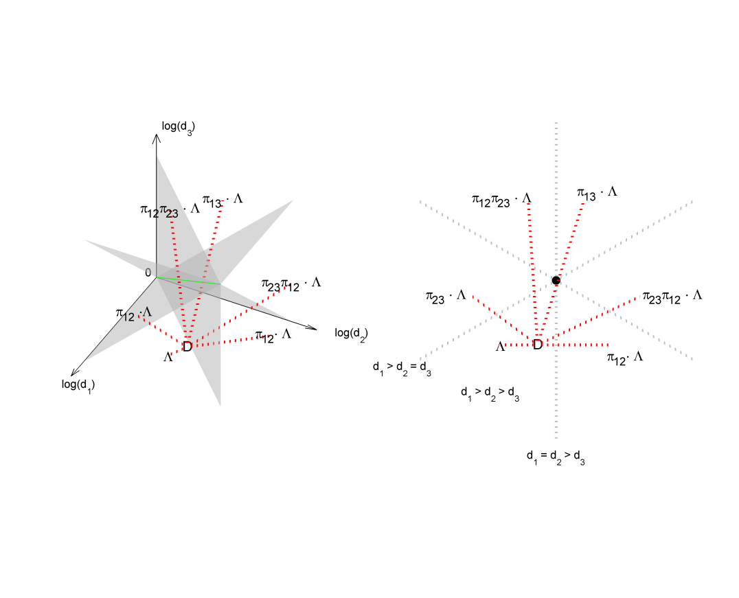
Figure 7: The space $\mbox{Diag}^{+}(3)$ with the line and planes representing the its stratification (left) and a cross section (right) of the stratified $\mbox{Diag}^{+}(3)$; see Fig. 3. For $D,\Lambda$ in the same connected component of $\mathcal{D}_{{\sf J}_{\rm top}}\subset\mbox{Diag}^{+}(3)$, the distance $d_{\mathcal{D}}(D,\Lambda)$ is represented by the “length” of the red dotted line. Also shown are $\pi_{g}\cdot\Lambda$ and $d_{\mathcal{D}}(D,\pi_{g}\cdot\Lambda)$ for all possible $\pi_{g}$. Here, we chose $D=\mbox{diag}(8,6,3)$, $\Lambda=\mbox{diag}(15,8,6)$.

In this example, because $\pi_{g}=\pi_{\rm id}$ gives the smallest $d_{\mathcal{D}}(D,\pi_{g}{\mbox{ \raisebox{-1.084pt}{\bf{\Large$\cdot$}}}}\Lambda)$, for sufficiently small $k$ the minimizer $g$ of (7.1) satisfies $\pi_{g}=\pi_{\rm id}$, and the ellipsoids corresponding to the MSSR curves from $t=0$ to $1$ are always tri-axial. For fixed $k$, other choices of $g$ can provide a minimal pair, depending on the values of $(U,D)$, $(V,\Lambda)$. Below, we list the shape-classification changes of the MSSR curve $\chi_{g}$ corresponding to the particular $g\in{\sf N}_{((U,D),(V,\Lambda))}\subset\tilde{S}^{+}_{3}$. A $3\times 3$ SPD matrix with eigenvalues $a\geq b\geq c$ has the shape of a sphere if $a=b=c$, oblate spheroid (or oblate, for short) if $a=b>c$, prolate spheroid (or prolate) if $a>b=c$, and tri-axial ellipsoid (or tri-axial) if $a>b>c$. We assume below that $D$ and $\Lambda$ have been chosen to lie in the same connected component of $\mathcal{D}_{{\sf J}_{\rm top}}$.

1. For all $g$ such that $\pi_{g}=\pi_{\rm id}$, for all $t\in[0,1]$, the ellipsoid corresponding to $\chi_{g}(t)$ is always tri-axial.

2. For all $g$ such that $\pi_{g}=\pi_{\rm 12}$, the shape-classification changes of the MSSR curves $\chi_{g}(t)$ from $t=0$ to $t=1$ are (tri-axial $\to$ oblate $\to$ tri-axial).

3. For all $g$ such that $\pi_{g}=\pi_{\rm 23}$, the shape-classification changes are (tri-axial $\to$ prolate $\to$ tri-axial).

4. For all $g$ such that $\pi_{g}=\pi_{\rm 123}$, the shape-classification changes are (tri-axial $\to$ oblate $\to$ tri-axial $\to$ prolate $\to$ tri-axial).

5. For all $g$ such that $\pi_{g}=\pi_{\rm 132}$, the shape-classification changes are (tri-axial $\to$ prolate $\to$ tri-axial $\to$ oblate $\to$ tri-axial).

6. For all $g$ such that $\pi_{g}=\pi_{\rm 13}$, the shape-classification changes are either
   (tri-ax. $\to$ oblate $\to$ tri-ax. $\to$ prolate $\to$ tri-ax. $\to$ oblate $\to$ tri-ax.),
   (tri-ax. $\to$ prolate $\to$ tri-ax. $\to$ oblate$\to$ tri-ax. $\to$ prolate $\to$ tri-ax.),
   or (tri-axial $\to$ sphere $\to$ tri-axial).

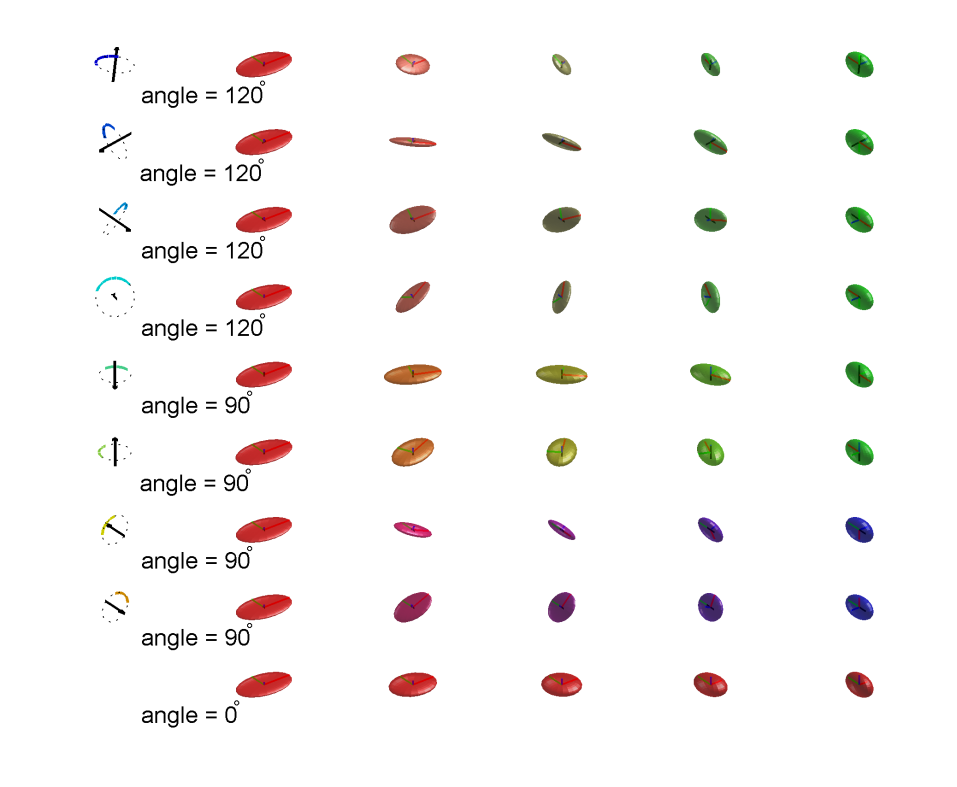
Figure 8: An example for one case of non-unique MSSR curves with $X,Y\in\mathcal{S}_{\rm top}$. There are nine MSSR curves. The rotation parameter $A$ of each MSSR curve is depicted as the axis-angle figure in the left-most panels. The top four MSSR curves correspond to the minimal pairs provided by $g$ with $\pi_{g}=\pi_{\rm id}$. The next two MSSR curves correspond to two choices of $g$ with $\pi_{g}=\pi_{12}$. The next two MSSR curves correspond to two choices of $g$ with $\pi_{g}=\pi_{23}$. The last MSSR curve corresponds to $g$ with $\pi_{g}=\pi_{123}$.

We close this section by providing the worst-case example of non-uniqueness we have found (for $X$ and $Y$ both having three distinct eigenvalues), in which there are 9 MSSR curves. We choose $X=\mbox{diag}(e^{a},e^{b},e^{c})$, where $c=1$, $b=c+\frac{7\sqrt{7}}{6\sqrt{8}}\pi$, $a=b+\sqrt{\frac{7}{72}}\pi$, and $Y=R\mbox{diag}(e^{x},e^{y},e^{z})R^{T}$ where $\phi^{-1}(R)=\frac{\pm 1}{2}(1+i+j+k)$ and $z=0$, $y=\frac{1}{3\sqrt{14}}\pi$, $x=y+\sqrt{\frac{7}{72}}\pi$. The nine MSSR curves are illustrated in Fig. 8. (See Section 5.1.1 for the definition of $\phi^{-1}(R)$.)

7.2 The case in which $X\in\mathcal{S}_{\rm mid}$ and $Y\in\mathcal{S}_{\rm top}$

For this special case, $X$ has just two distinct eigenvalues, while $Y$ has three. We parameterize $X$ with $a,b\in\mathbf{R}$ (arbitrary, not size-ordered), and any $U\in\mbox{SO}(3)$, and parameterize $Y$ with $c>d>f>0$ and a unit quaternion $q=z+wj\in S_{\mathbf{H}}^{3}$, where $z,w\in\mathbf{C}$ and, $|z|^{2}+|w|^{2}=1$, as follows:

$$X=U\begin{pmatrix}e^{a}&0&0\\ 0&e^{b}&0\\ 0&0&e^{b}\\ \end{pmatrix}U^{T},\quad Y=U\phi(q)\begin{pmatrix}e^{c}&0&0\\ 0&e^{d}&0\\ 0&0&e^{f}\\ \end{pmatrix}(U\phi(q))^{T}$$ (7.3)

where $\phi:S_{\mathbf{H}}^{3}\to\mbox{SO}(3)$ is the natural two-to-one Lie-group homomorphism defined in Section 5.1.1. Without loss of generality, we assume $\mbox{Re}(q)=\mbox{Re}(z)>0$ so that $\phi(q)$ is not an involution.

There are six different cases of MSSR curves as summarized in Table 4, named ${\rm A}_{1},{\rm A}_{2},{\rm B}_{1},{\rm B}_{2},{\rm C}_{1},{\rm C}_{2}$. To give representative examples of these cases, we partially rewrite the conditions in Table 6.2.

Recall that $\varphi=\cos^{-1}(\max\{|z|,|w|\})\in[0,\frac{\pi}{4}]$. For each $\varphi\in(0,\pi/4)$ there are exactly two cases: $\cos(\varphi)=|z|>|w|$ and $|z|<|w|=\cos(\varphi)$. If $\varphi=0$, then $|z|=1,|w|=0$. If $\varphi=\frac{\pi}{4}$, then $|z|=|w|=1/\sqrt{2}$. We define

$$\alpha=\left\{\begin{array}[]{ll}\cos^{-1}\left(\frac{|{\rm Re}(\bar{z}w)|}{|\bar{z}w|}\right),&\hbox{if $\varphi>0$;}\\ \pi/2,&\hbox{if $\varphi=0$,}\end{array}\right.\in[0,\frac{\pi}{2}],$$ (7.4)

so that the parameters $\beta$ and $\beta^{\prime}$ appearing in Theorem 5.4 and Table 6.2 will be represented by

$$\beta =\frac{1}{2}\cos^{-1}(\sin(2\varphi)\cos\alpha)\in[0,\frac{\pi}{4}],$$ (7.5)

$$\beta^{\prime} =\frac{1}{2}\cos^{-1}(\sin(2\varphi)\sin\alpha)\in[0,\frac{\pi}{4}].$$ (7.6)

Note that

$$\varphi=0\ \Longleftrightarrow\ |z|=1\ \Longleftrightarrow\ \beta=\beta^{\prime}=\frac{\pi}{4}$$ (7.7)

and that

$$\mbox{Re}(\bar{z}w)=0\ \Longleftrightarrow\ \cos\alpha=0\ \Longleftrightarrow\ \alpha=\frac{\pi}{2},$$ (7.8)

$$\mbox{Im}(\bar{z}w)=0\ \Longleftrightarrow\ \cos\alpha=1\ \Longleftrightarrow\ \alpha=0.$$ (7.9)

For any $\alpha<\pi/2$, $\mbox{Re}(\bar{z}w)$ can have either sign. For $\alpha>0$, $\mbox{Im}(\bar{z}w)$ can have either sign.

We also make use of the following parameters, concerning the eigenvalues of $X$ and $Y$, scaled by $k$ (where $k>0$ is as in (3.4)):

$$m_{1}=\frac{2(a-b)(c-d)}{4k},\quad m_{2}=\frac{2(a-b)(d-f)}{4k}.$$ (7.10)

Each of $m_{1}$ and $m_{2}$ can be either positive or negative, but they must both have the same sign. To simplify the analysis, we assume

$$m_{1}=m_{2}:=m^{\prime}.$$ (7.11)

Then we have

$$\ell^{2}_{\rm id} <\ell^{2}_{13}\ \Longleftrightarrow\ \varphi^{2}-\beta^{2}-2m^{\prime}<0,$$ (7.12)

$$\ell^{2}_{\rm id} <\ell^{2}_{12}\ \Longleftrightarrow\ \varphi^{2}-(\beta^{\prime})^{2}-m^{\prime}<0,$$ (7.13)

$$\ell^{2}_{13} <\ell^{2}_{12}\ \Longleftrightarrow\ \beta^{2}-(\beta^{\prime})^{2}+m^{\prime}<0.$$ (7.14)

By (7.5), (7.12) is equivalent to

$$\alpha>\cos^{-1}\left(\frac{\cos(2\sqrt{(\varphi^{2}-2m^{\prime})_{+}})}{\sin(2\varphi)}\right),\quad\mbox{ if }\varphi>0,$$

and to $m^{\prime}>-\frac{\pi^{2}}{32}$ if $\varphi=0$. By (7.6), (7.13) is equivalent to

$$\alpha<\sin^{-1}\left(\frac{\cos(2\sqrt{(\varphi^{2}-m^{\prime})_{+}})}{\sin(2\varphi)}\right),\quad\mbox{ if }\varphi>0,$$

and to $m^{\prime}>-\frac{\pi^{2}}{16}$ if $\varphi=0$. We have not found a similarly simple inequality equivalent to (7.14). Figure 9, generated numerically, indicates the regions of $(\varphi,\alpha)$ corresponding to different size-orders of $\ell_{\rm id},\ell_{13},\ell_{12}$, for the fixed value $m^{\prime}=-0.1$. The seven cases of unique and non-unique MSSR curves summarized in Table 6.2 are graphically represented in Figs. 10 and 11. As $|m^{\prime}|$ increases, either ${\rm A}_{l}$ or ${\rm B}_{m}$ becomes the only case of MSSR curves.

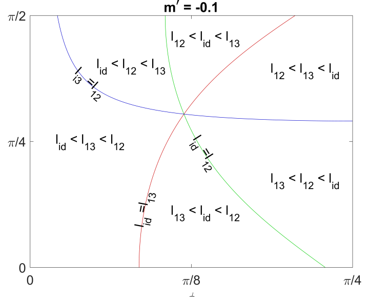
Figure 9: The ordering of $\ell_{\rm id},\ell_{13},\ell_{12}$ corresponding to the value of $(\varphi,\alpha)\in[0,\pi/4]\times[0,\pi/2]$. Note that $m^{\prime}=-0.1$ is fixed.

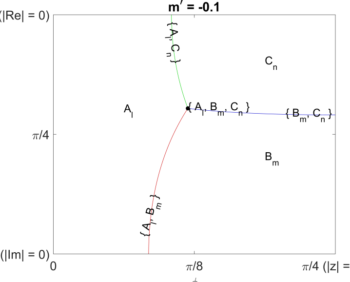
Figure 10: Cases of unique and non-unique MSSR curves in $\mbox{Sym}^{+}(3)$ when $X$ has just two distinct eigenvalues, and $Y$ has three distinct eigenvalues. This figure uses the same parametrization of Fig. 9, with $m^{\prime}=-0.1$. The case ${\rm A}_{l}$ stands for either ${\rm A}_{1}$ (if $|z|>|w|$), ${\rm A}_{2}$ (if $|z|<|w|$) or $\{{\rm A}_{1},{\rm A}_{2}\}$ (if $|z|=|w|$). The latter case ($|z|=|w|$) can only occur if $\varphi=\pi/4$. The case ${\rm B}_{m}$ stands for either ${\rm B}_{1}$ (if $\mbox{Re}(\bar{z}w)>0$), ${\rm B}_{2}$ (if $\mbox{Re}(\bar{z}w)<0$), or $\{{\rm B}_{1},{\rm B}_{2}\}$ (if $\mbox{Re}(\bar{z}w)=0$). The latter case ($\mbox{Re}(\bar{z}w)=0$) can only occur if $\alpha=\pi/2$. Similarly, the case ${\rm C}_{n}$ stands for either ${\rm C}_{1}$ (if $\mbox{Im}(\bar{z}w)>0$), ${\rm C}_{2}$ (if $\mbox{Im}(\bar{z}w)<0$), or $\{{\rm C}_{1},{\rm C}_{2}\}$ (if $\mbox{Im}(\bar{z}w)=0$). The latter case ($\mbox{Im}(\bar{z}w)=0$) can only occur if $\alpha=0$. The multi-element cases such as $\{{\rm A}_{l},{\rm B}_{m}\}$ can be understood similarly. The values of $l$ and $m$ are determined by the signs of $|z|-|w|$ and $\mbox{Re}(\bar{z}w)$, and if there are two values for $l$ and one value for $m$, then the case is $\{{\rm A}_{1},{\rm A}_{2},{\rm B}_{m}\}$, a case with three MSSR curves.

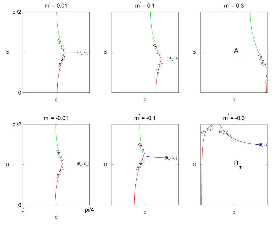
Figure 11: Unique and non-unique MSSR curves in $\mbox{Sym}^{+}(3)$ when $X$ has just two distinct eigenvalues, and $Y$ has three distinct eigenvalues.

In the following we provide several examples of the unique and non-unique cases of MSSR curves for the case $X\in\mathcal{S}_{\rm mid}$ and $Y\in\mathcal{S}_{\rm top}$. We first discuss the shape classification changes of the scaling-rotation curves $\chi_{{\rm A}_{l}}(t)$, $\chi_{{\rm B}_{m}}(t)$ and $\chi_{{\rm C}_{n}}(t)$ $(l,m,n=1,2)$. These depend on the sign of $m^{\prime}$.

1. If $m^{\prime}>0$ (that is, $X$ is prolate, and $Y$ is tri-axial), then the shape-classification changes of $\chi_{{\rm A}_{l}}(t)$ are (prolate $\to$ tri-axial); for $\chi_{{\rm B}_{m}}(t)$ they are (prolate $\to$ tri-axial $\to$ oblate $\to$ tri-axial $\to$ prolate $\to$ tri-axial); for $\chi_{{\rm C}_{n}}(t)$ they are (prolate $\to$ tri-axial $\to$ oblate $\to$ tri-axial).

2. If $m^{\prime}<0$ (that is, $X$ is oblate, and $Y$ is tri-axial), then the shape-classification changes of $\chi_{{\rm A}_{l}}(t)$ are (oblate $\to$ tri-axial $\to$ prolate $\to$ tri-axial $\to$ oblate $\to$ tri-axial); for $\chi_{{\rm B}_{m}}(t)$ they are (oblate $\to$ tri-axial); for $\chi_{{\rm C}_{n}}(t)$ they are (oblate $\to$ tri-axial $\to$ prolate $\to$ tri-axial).

Two scaling-rotation curves ${\rm A}_{1}$ and ${\rm A}_{2}$ (or ${\rm B}_{1}$ and ${\rm B}_{2}$, ${\rm C}_{1}$ and ${\rm C}_{2}$) share the same scaling parameters, and also share the same rotation axis, but with different orientations (one clockwise, the other counterclockwise) and possibly different angles. The two angles differ by $\pi$.

In an attempt to visually illustrate examples in Fig. 12 to Fig. 14, a scaling-rotation curve $\chi:=\chi_{U,D,A,L}$ in the 6-dimensional space $\mbox{Sym}^{+}(3)$ is depicted by both a sequence of ellipsoids (representing the discretized scaling-rotation curve $\chi$) and the combination of the rotation parameter $A$ and changes of eigenvalues $D\exp(Lt)$. The rotation parameters $A$ of $\chi$ are depicted as the axis-angle figure in the top left-most panels of figures below. The bottom panel of each figure depicts a logarithmic projection to $\mbox{Diag}(3)$ of the curve $D\exp(Lt)\in\mbox{Diag}^{+}(3)$ from $D$ (black dot) to $D\exp(L)$ (red dots). (See Fig. 3 for the definition of shaded planes.) Since the rotational degrees of freedom have been projected out in the bottom panel, the relative lengths of the straight-line-segments do not accurately reflect the relative lengths of the curves.

We collect representative visual examples in which there are a unique MSSR curve (Fig. 12, the case $\{{\rm A}_{1}\}$), exactly two MSSR curves (Fig. 13, the case $\{{\rm A}_{1},{\rm B}_{1}\}$), and exactly three MSSR curves (Fig. 14, the case $\{{\rm A}_{1},{\rm B}_{1},{\rm C}_{1}\}$). More situations, including a four-MSSR-curve case, are possible.

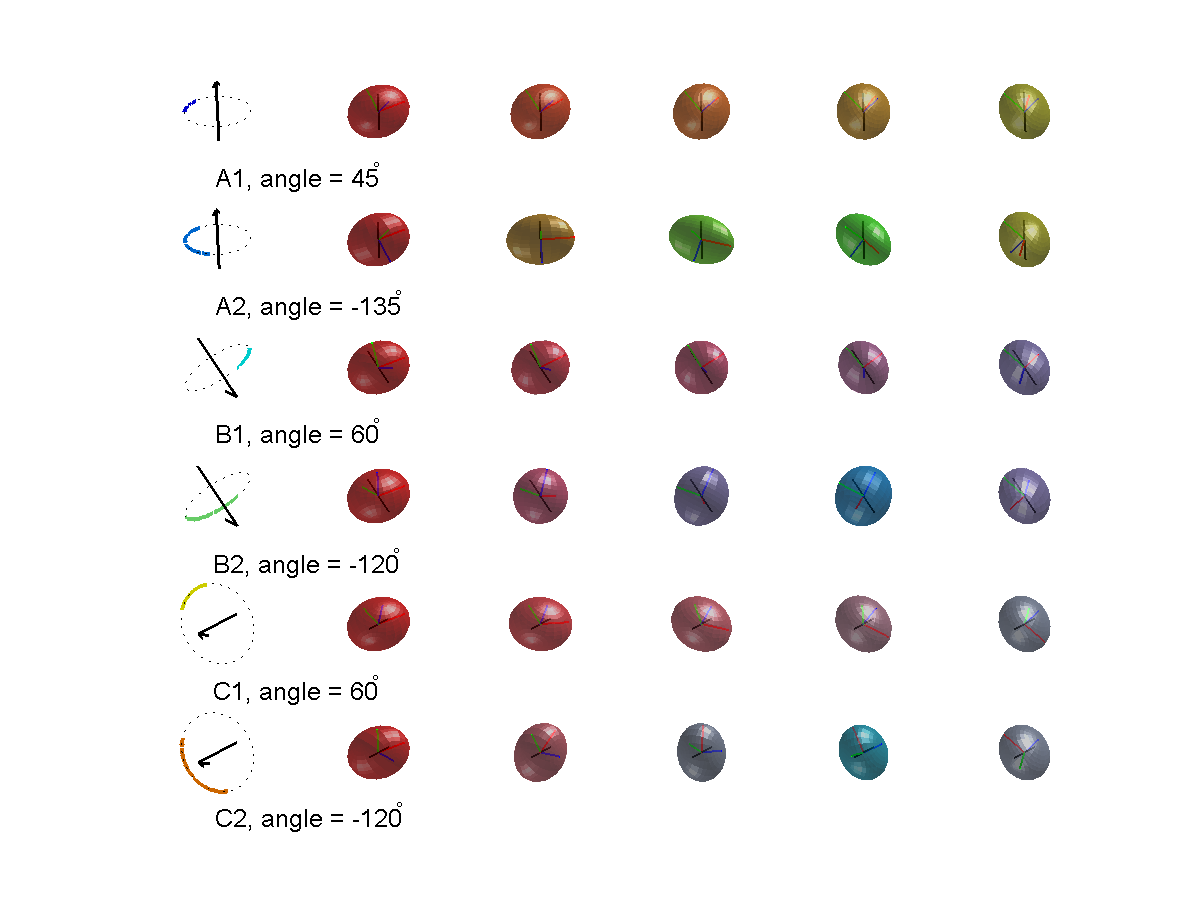
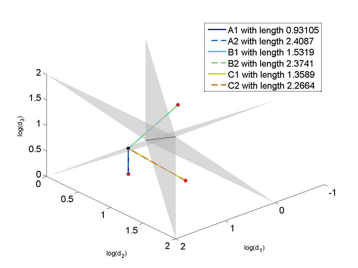
Figure 12: An example for the case $\{{\rm A}_{1}\}$. (The scaling-rotation curve corresponding to ${\rm A}_{1}$ is the unique MSSR curve.) Each of the cases ${\rm A}_{1}$ - ${\rm C}_{2}$ represents the corresponding scaling-rotation curve defined in Table 4, whose length can be found in the legend. Note that $m^{\prime}>0$ in this example. The eigenvalue paths corresponding to ${\rm A}_{1}$ and ${\rm A}_{2}$ depart from a single connected component of $\mathcal{D}_{{\sf J}_{1}}$ (represented by the shaded open half-plane containing the black dot) and reach $\mathcal{D}_{\rm top}$. Accordingly, the shape-classification changes are (prolate $\to$ tri-axial).

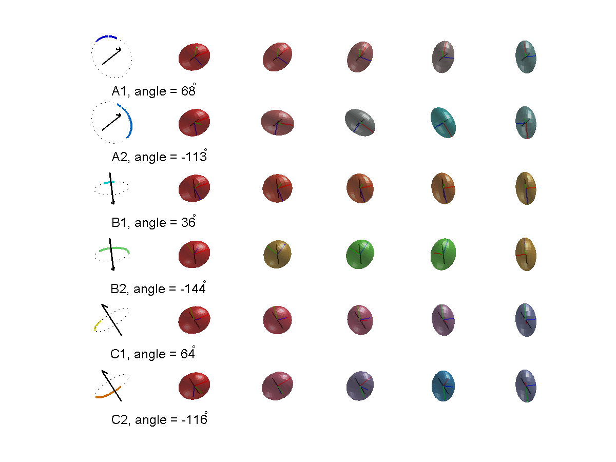
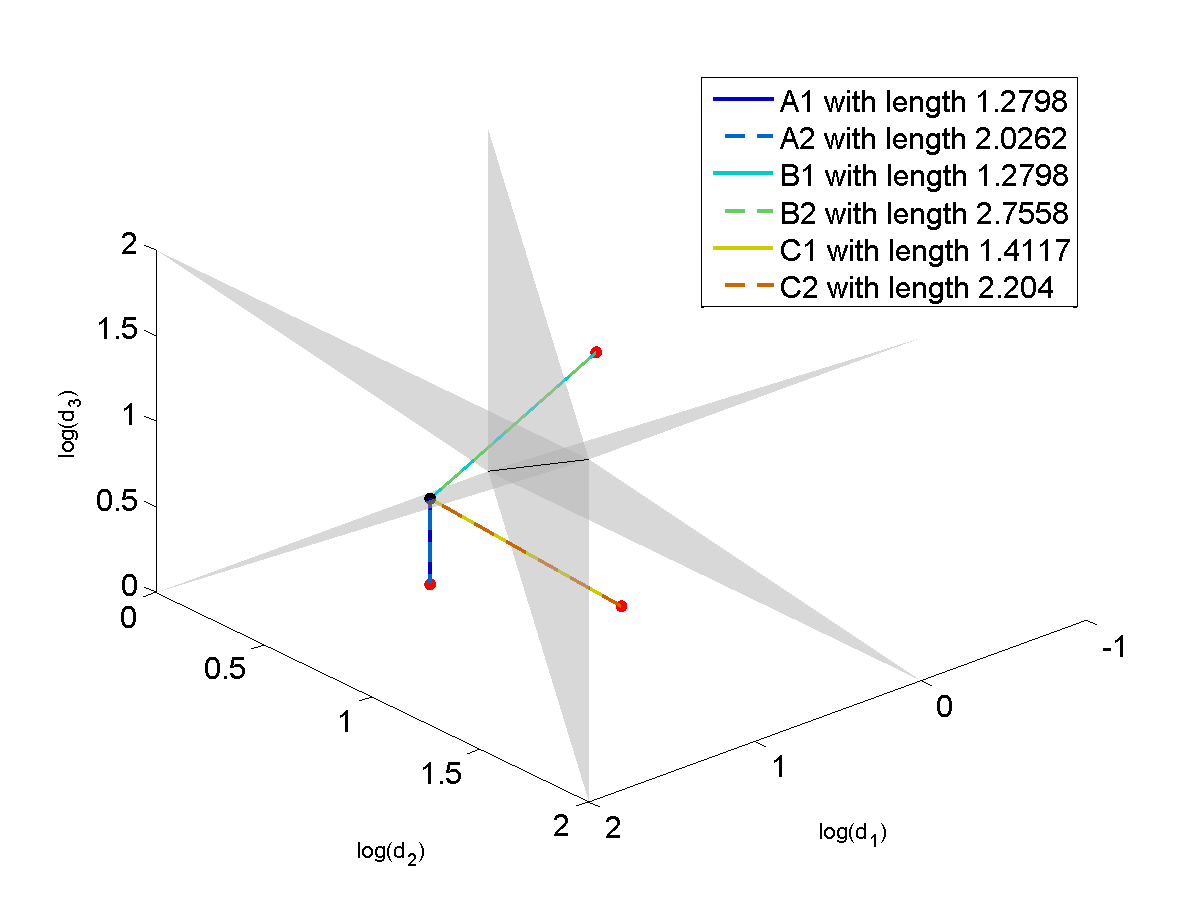
Figure 13: An example for the case $\{{\rm A}_{1},{\rm B}_{1}\}$.

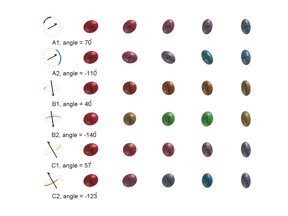
Figure 14: An example for the case $\{{\rm A}_{1},{\rm B}_{1},{\rm C}_{1}\}$.

7.3 The case in which both $X$ and $Y$ have exactly two distinct eigenvalues

For this special case, we parameterize $X$ and $Y$ with $a,b,c,d\in\mathbf{R}$ (not ordered), and a unit quaternion $q=z+wj\in S_{\mathbf{H}}^{3}$, where $z,w\in\mathbf{C}$, $|z|^{2}+|w|^{2}=1$ as

$$X=U\begin{pmatrix}e^{a}&0&0\\ 0&e^{b}&0\\ 0&0&e^{b}\\ \end{pmatrix}U^{T},\quad Y=U\phi(q)\begin{pmatrix}e^{c}&0&0\\ 0&e^{d}&0\\ 0&0&e^{d}\\ \end{pmatrix}(U\phi(q))^{T}$$ (7.15)

where $U\in\mbox{SO}(3)$. Without loss of generality, we assume $\mbox{Re}(q)=\mbox{Re}(z)>0$ so that $\phi(q)$ is not an involution.

There are four different cases of MSSR curves arising from the parametrization of (7.15), as summarized in Table 4. These cases are denoted ${\rm A}_{1}^{\prime},{\rm A}_{2}^{\prime},{\rm B}^{\prime}$ and ${\rm C}^{\prime}$. Our goal here is to further investigate the seven subcases of $\mathcal{M}(X,Y)$ in Table 6, by partially rewriting the conditions in Table 6. Note that $0<|z|\leq 1$, $0\leq\cos^{-1}|z|<\frac{\pi}{2}$, $|w|=\sqrt{1-|z|^{2}}=\cos(\frac{\pi}{2}-\cos^{-1}|z|)$, and

$$\varphi =\cos^{-1}(\max\{|z|,|w|\})=\min\{\cos^{-1}|z|,\cos^{-1}(\sqrt{1-|z|^{2}})\}$$

$$=\left\{\begin{array}[]{ll}\cos^{-1}|z|,&0\leq\cos^{-1}|z|\leq\frac{\pi}{4};\\ \frac{\pi}{2}-\cos^{-1}|z|,&\frac{\pi}{4}\leq\cos^{-1}|z|<\frac{\pi}{2}.\end{array}\right.$$ (7.18)

Let $m=\frac{2(a-b)(c-d)}{k\pi}.$ Unlike in the $\mbox{Sym}^{+}(2)$ case (cf. Section 4), this $m$ can be either positive or negative, but not zero. If $X$ and $Y$ are both prolates (or both oblates), then $m>0$. If $X$ is an oblate and $Y$ is a prolate (or vice versa), then $m<0$. By Theorem 5.4,

$$\ell_{\rm id}<\ell_{13}\ \Longleftrightarrow\ m>2(\varphi-\frac{\pi}{8}).$$ (7.19)

Moreover,

$$|z|>|w|\ \Longleftrightarrow\ \frac{1}{\sqrt{2}}<|z|\leq 1\ \Longleftrightarrow\ 0\leq\cos^{-1}|z|<\frac{\pi}{4}$$ (7.20)

$$|z|<|w|\ \Longleftrightarrow\ 0<|z|<\frac{1}{\sqrt{2}}\ \Longleftrightarrow\ \frac{\pi}{4}<\cos^{-1}|z|<\frac{\pi}{2}$$ (7.21)

Combining (7.18)-(7.21), the conditions for the nine subcases in Table 6 are represented by $m\neq 0$ and $\cos^{-1}|z|\in[0,\frac{\pi}{2})$, as shown in Fig. 15. These subcases can be sub-divided by the sign of $m$.

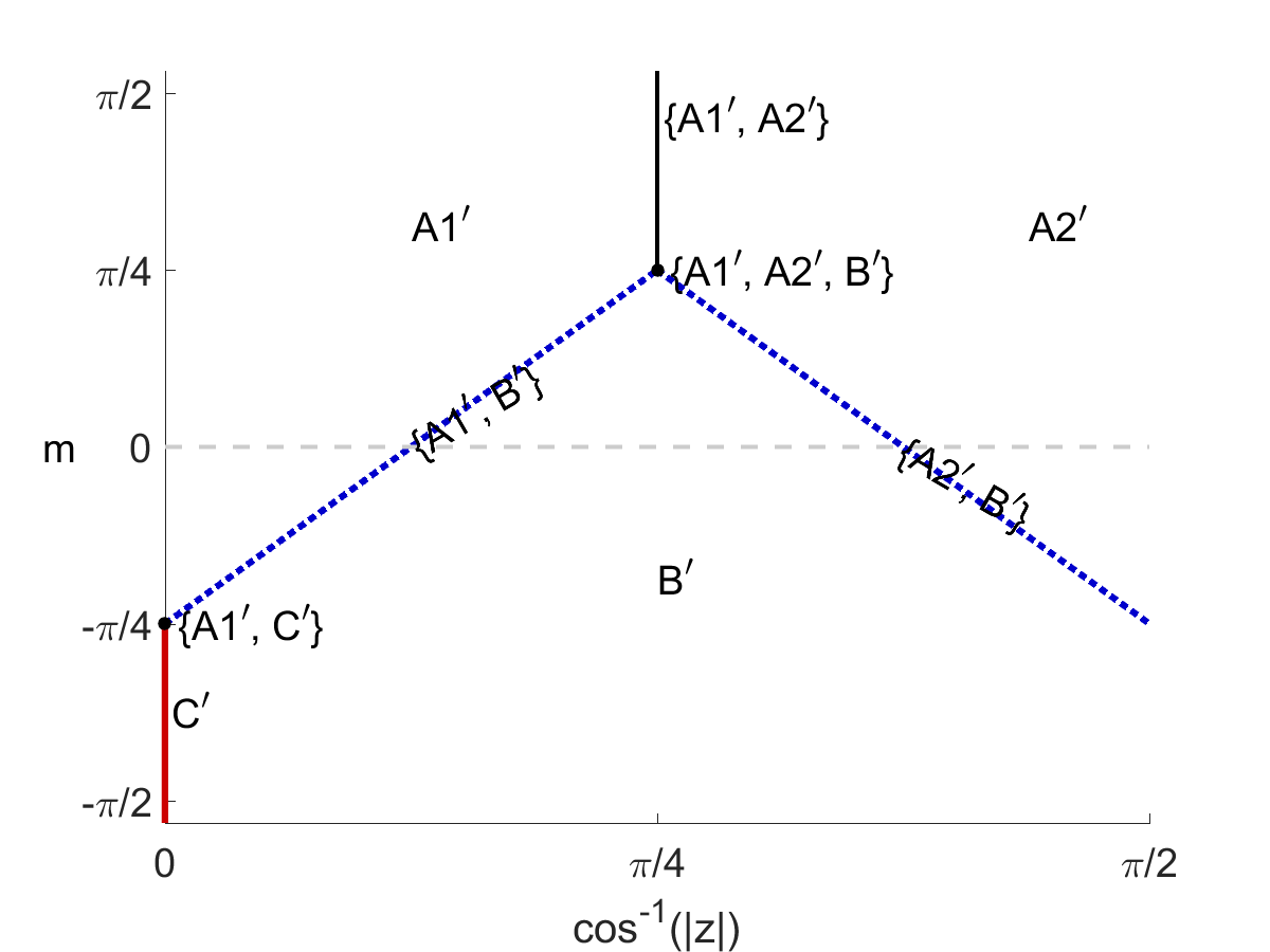
Figure 15: Unique and non-unique MSSR curves in $\mbox{Sym}^{+}(3)$ when both $X$ and $Y$ have exactly two distinct eigenvalues: Schematic illustration for the nine subcases. The horizontal line $m=0$ is excluded.

In the following we take a few representative examples of the nine subcases. Each example of MSSR curve $\chi$ is accompanied by its shape-classification changes. Note that the seven subcases not involving ${\rm C}^{\prime}$ resemble the seven subcases of $p=2$; see Section 4. The case ${\rm C}^{\prime}$ is only defined for $|z|=1$ (or $\cos^{-1}|z|=0$), in which situations the cases ${\rm A}_{2}^{\prime}$, ${\rm B}_{1}$ are not defined.

1. $\{{\rm A}_{1}^{\prime}\}$. Unique MSSR curve $\chi$. If $m>0$, the shapes of $\chi(t)$ are always prolate (or oblate) for all $t\in[0,1]$; if $m<0$, the shape-classification changes of the MSSR curve $\chi(t)$ evaluated from $t=0$ to $t=1$ are either (oblate $\to$ sphere$\to$ prolate) or (prolate $\to$ sphere $\to$ oblate). See Fig. 16 for an example with $m>0$.

2. $\{{\rm B}^{\prime}\}$. Unique MSSR curve. For prolate $X$, the shape-classification changes are (prolate $\to$ tri-axial $\to$ oblate $\to$ tri-axial $\to$ prolate) if $m>0$, (prolate $\to$ tri-axial $\to$ oblate) if $m<0$. For oblate $X$, interchange “oblate” and “prolate” in these shape-classification changes.

3. $\{{\rm A}_{1}^{\prime},{\rm A}_{2}^{\prime}\}$. Two MSSR curves with rotation angle $\pi/2$. The shape-classification changes of ${\rm A}_{2}^{\prime}$ are the same as those of ${\rm A}_{1}^{\prime}$, and dependent on the sign of $m$; see item 1.

4. $\{{\rm A}_{1}^{\prime},{\rm A}_{2}^{\prime},{\rm B}^{\prime}\}$. Three MSSR curves (two with rotation angle $\pi/2$ and the other involving no rotation).

5. $\{{\rm C}^{\prime}\}$. Uncountably many MSSR curves. See Fig. 17. The set of MSSR curves is in natural one-to-one correspondence with $S_{\mathbb{C}}^{1}$. In this case $m<0$, and the corresponding shape changes are the same as the case $\{B^{\prime}\}$, with $m<0$: (prolate $\to$ tri-axial $\to$ oblate).

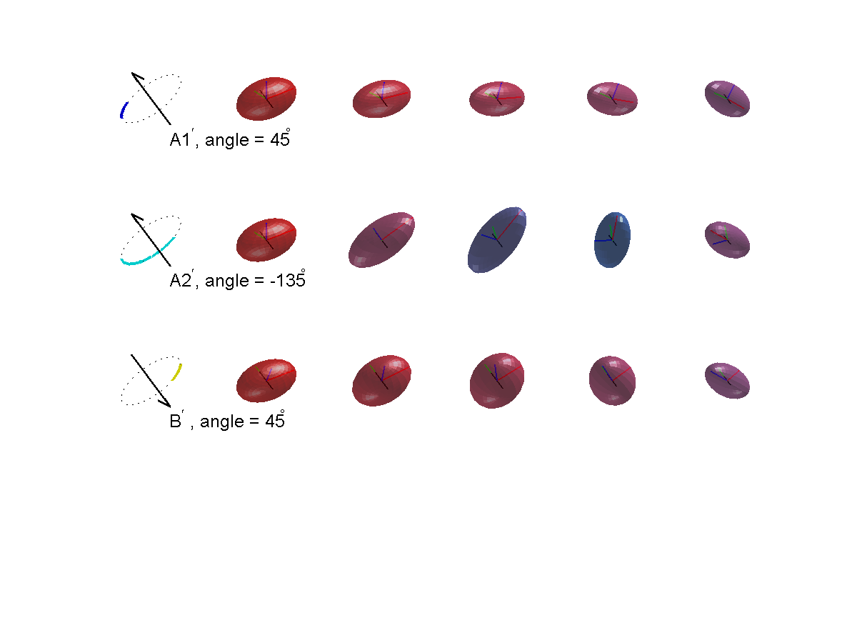
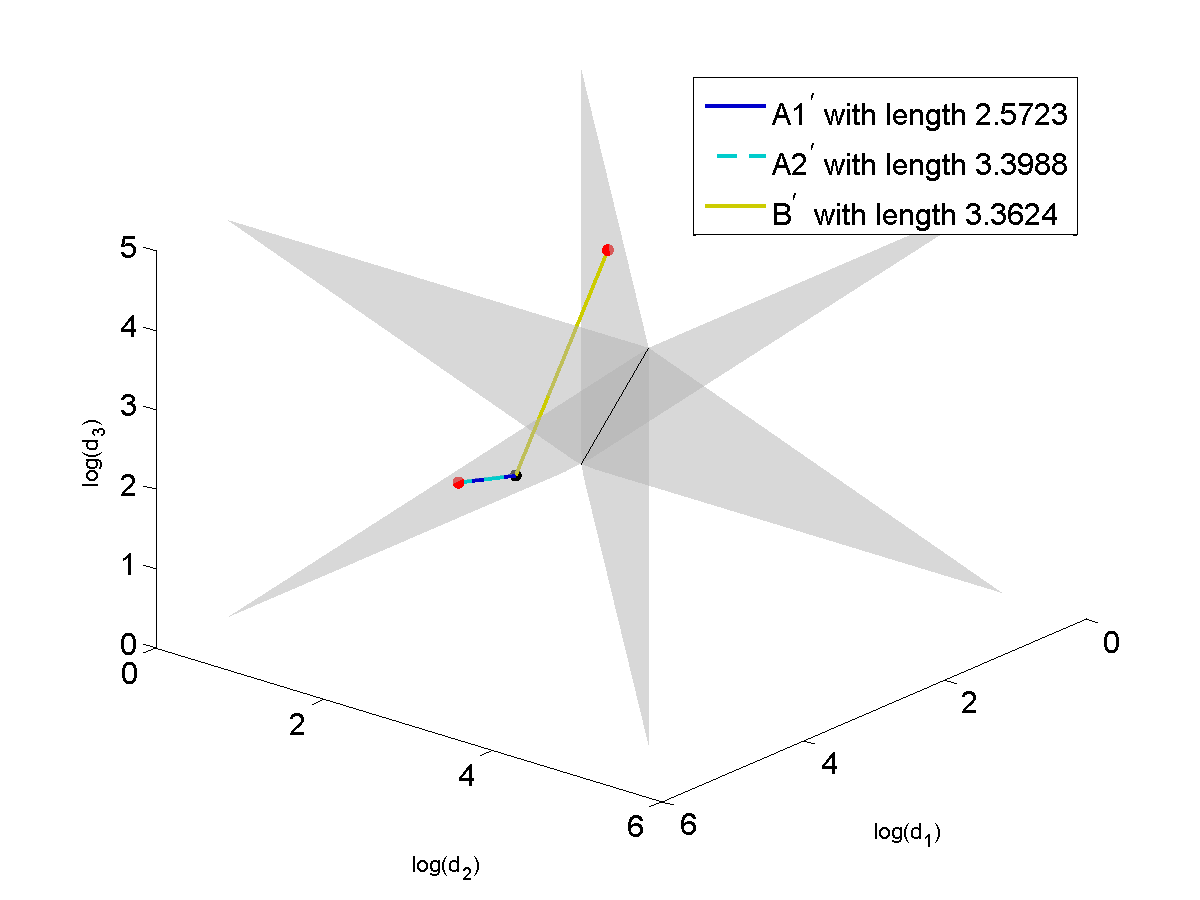
Figure 16: An example for the case $\{{\rm A}_{1}^{\prime}\}$ (The scaling-rotation curve corresponding to ${\rm A}_{1}^{\prime}$ is the unique MSSR curve.) Each of the cases ${\rm A}_{1}^{\prime}$, ${\rm A}_{2}^{\prime}$, and ${\rm B}^{\prime}$ represents the corresponding scaling-rotation curves defined in Table 4, whose length can be found in the legend. Since the rotational degrees of freedom have been projected out in the bottom panel, the relative lengths of the straight-line segments do not accurately reflect the relative lengths of the curves. Note that $m>0$ in this example. The eigenvalue paths corresponding to ${\rm A}_{1}^{\prime}$ and ${\rm A}_{2}^{\prime}$ stay in a single connected component of $\mathcal{D}_{{\sf J}_{1}}$ (represented by one of the shaded open half-planes) and their shapes are all prolates (if both $X$ and $Y$ are prolates) or all oblates (if both $X$ and $Y$ are oblates). On the other hand, the eigenvalue path corresponding to ${\rm B}^{\prime}$ travels through $\mathcal{D}_{\rm top}$ and another shaded plane corresponding to ${\sf J}_{2}$. That is, the shape-classification changes are (prolate $\to$ tri-axial $\to$ oblate $\to$ tri-axial $\to$ prolate).

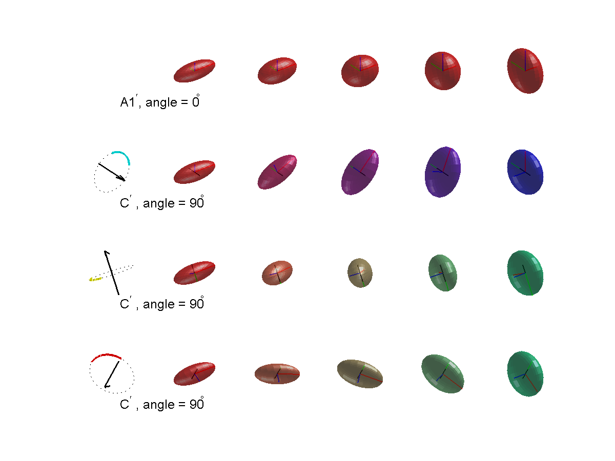
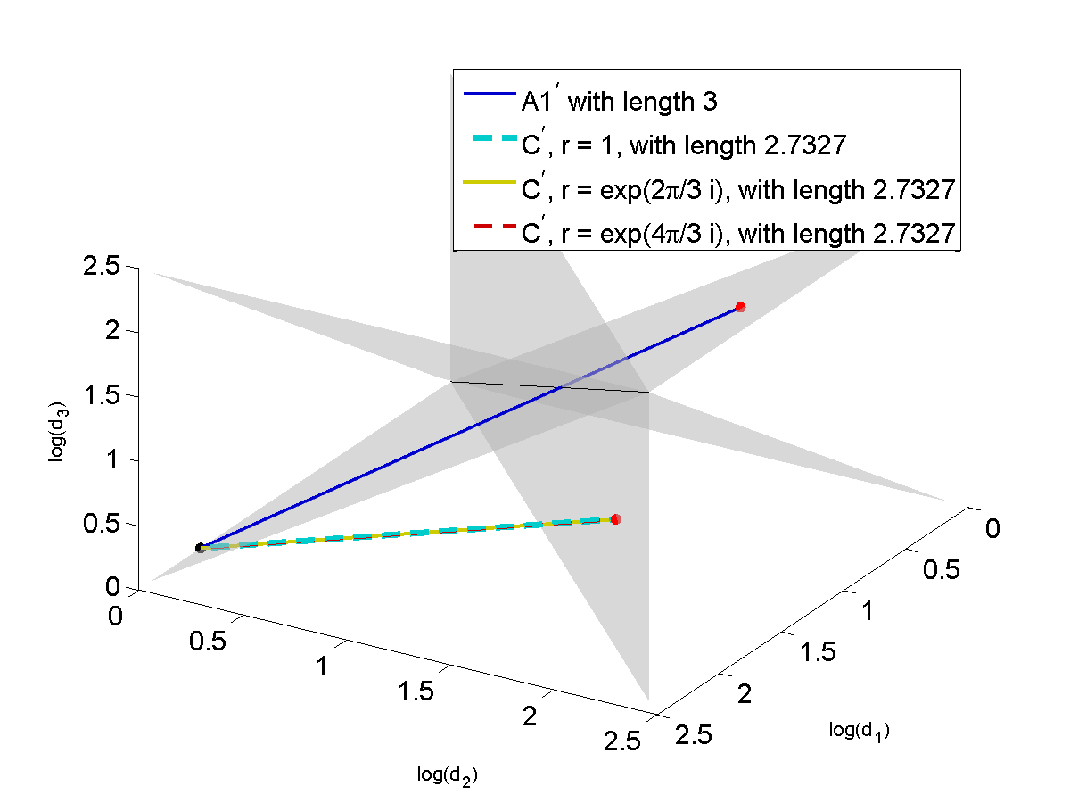
Figure 17: An example for the case $\{\rm{}C^{\prime}\}$. For each of the case ${\rm C}^{\prime}$, the rotation axis (depicted as the black line segment) is orthogonal to the (red) major semi-axis of $X$. It is shown in the proof of Theorem 6.2(i) that there is one-to-one correspondence between the “equator” of $X$ and the family $\mathcal{M}_{{\rm C}^{\prime}}$; see also Remark 6.4.

References

- [1] P-A Absil, Robert Mahony, and Rodolphe Sepulchre. Optimization algorithms on matrix manifolds. Princeton University Press, 2009.
- [2] Daniel C Alexander. Multiple-fiber reconstruction algorithms for diffusion MRI. Annals of the New York Academy of Sciences, 1064(1):113–133, 2005.
- [3] Vincent Arsigny, Pierre Fillard, Xavier Pennec, and Nicholas Ayache. Geometric means in a novel vector space structure on symmetric positive-definite matrices. SIAM J. Matrix Anal. Appl., 29(1):328–347, 2007.
- [4] Burcu Aydin, Gabor Pataki, Haonan Wang, Elizabeth Bullitt, and James Stephen Marron. A principal component analysis for trees. The Annals of Applied Statistics, pages 1597–1615, 2009.
- [5] Miroslav Bacák. Computing medians and means in Hadamard spaces. SIAM Journal on Optimization, 24(3):1542–1566, 2014.
- [6] Dennis Barden, Huiling Le, and Megan Owen. Limiting behaviour of Fréchet means in the space of phylogenetic trees. To appear in Annals of the Institute of Statistical Mathematics, 2017. doi:10.1007/s10463-016-0582-9
- [7] Dennis Barden, Huiling Le, Megan Owen, et al. Central limit theorems for Fréchet means in the space of phylogenetic trees. Electron. J. Probab, 18(25):1–25, 2013.
- [8] Rabi Bhattacharya and Lizhen Lin. Omnibus CLTs for Fréchet means and nonparametric inference on non-Euclidean spaces. Proc. Amer. Math. Soc., 145:413–428, 2017.
- [9] Philip Bille. A survey on tree edit distance and related problems. Theoretical computer science, 337(1):217–239, 2005.
- [10] Louis J. Billera, Susan P. Holmes, and Karen Vogtmann. Geometry of the space of phylogenetic trees. Adv. in Appl. Math., 27(4):733–767, 2001.
- [11] A. A. du Plessis E. J. N. Looijenga C. G. Gibson, K. Wirthmüller. Topological Stability of Smooth Mappings, volume 552 of Lecture Notes in Mathematics, Springer-Verlag, Berlin, 1976.
- [12] John Chakerian and Susan Holmes. Computational tools for evaluating phylogenetic and hierarchical clustering trees. Journal of Computational and Graphical Statistics, 21(3):581–599, 2012.
- [13] James Damon and J. S. Marron. Backwards principal component analysis and principal nested relations. Journal of Mathematical Imaging and Vision, 50(1-2):107–114, 2014.
- [14] I. L. Dryden, A. Koloydenko, and D. Zhou. Non-Euclidean statistics for covariance matrices, with applications to diffusion tensor imaging. Annals of Applied Statistics, 3:1102–1123, 2009.
- [15] Aasa Feragen. Complexity of computing distances between geometric trees. In Joint IAPR International Workshops on Statistical Techniques in Pattern Recognition (SPR) and Structural and Syntactic Pattern Recognition (SSPR), 89–97. Springer, 2012.
- [16] Aasa Feragen, Stephan Huckemann, J. S. Marron, and Ezra Miller. Mini-workshop: Asymptotic statistics on stratified spaces. Oberwolfach Reports, 11(4):2481–2527, 2014.
- [17] Aasa Feragen, Pechin Lo, Marleen de Bruijne, Mads Nielsen, and François Lauze. Toward a theory of statistical tree-shape analysis. IEEE transactions on pattern analysis and machine intelligence, 35(8):2008–2021, 2013.
- [18] Mario Forni, Marc Hallin, Marco Lippi, and Lucrezia Reichlin. The generalized dynamic-factor model: Identification and estimation. Review of Economics and Statistics, 82(4):540–554, 2000.
- [19] M. Goresky and R. MacPherson. Stratified Morse Theory. Springer-Verlag, Berlin Heidelberg, 1988.
- [20] David Groisser, Sungkyu Jung, and Armin Schwartzman. Foundations of scaling-rotation geometry for the space of symmetric positive-definite matrices. Preprint, arXiv:1702.03237, 2017.
- [21] Godfrey H. Hardy and Edward M. Wright. An Introduction to the Theory of Numbers. Oxford University Press, 1979.
- [22] Thomas Hotz, Stephan Huckemann, Huiling Le, J. S. Marron, Jonathan C. Mattingly, Ezra Miller, James Nolen, Megan Owen, Vic Patrangenaru, and Sean Skwerer. Sticky central limit theorems on open books. Ann. Appl. Probab., 23(6):2238–2258, 2013.
- [23] Stephan Huckemann, Thomas Hotz, and Axel Munk. Intrinsic shape analysis: Geodesic PCA for Riemannian manifolds modulo isometric Lie group actions. Statistica Sinica, 20(1):1–58, 2010.
- [24] D. G. Ebin J. Cheeger. Comparison Theorems in Riemannian Geometry. North Holland/American Elsevier, Amsterdam, 1975.
- [25] Sungkyu Jung, Armin Schwartzman, and David Groisser. Scaling-rotation distance and interpolation of symmetric positive definite matrices. Siam J. Matrix Anal. Appl., 36(3):1180–1201, 2015.
- [26] D. G. Kendall, D. Barden, T. K. Carne, and H. Le. Shape and shape theory. Wiley Series in Probability and Statistics. John Wiley & Sons Ltd., Chichester, 1999.
- [27] Christophe Lenglet, Mikaël Rousson, and Rachid Deriche. DTI segmentation by statistical surface evolution. IEEE Transactions on Medical Imaging, 25(6):685–700, 2006.
- [28] Ezra Miller, Megan Owen, and J Scott Provan. Polyhedral computational geometry for averaging metric phylogenetic trees. Advances in Applied Mathematics, 68:51–91, 2015.
- [29] Maher Moakher. A differential geometric approach to the geometric mean of symmetric positive-definite matrices. SIAM J. Matrix Anal. Appl., 26(3):735–747 (electronic), 2005.
- [30] Tom M.W. Nye. Principal components analysis in the space of phylogenetic trees. The Annals of Statistics, pages 2716–2739, 2011.
- [31] Tom M.W. Nye. Convergence of random walks to Brownian motion in phylogenetic tree-space. arXiv preprint arXiv:1508.02906, 2016.
- [32] Tom M.W. Nye and M.C. White. Diffusion on some simple stratified spaces. Journal of mathematical imaging and vision, 50(1-2):115–125, 2014.
- [33] Daniel Osborne, Vic Patrangenaru, Leif Ellingson, David Groisser, and Armin Schwartzman. Nonparametric two-sample tests on homogeneous Riemannian manifolds, Cholesky decompositions and diffusion tensor image analysis. J. Multivariate Anal., 119:163–175, 2013.
- [34] Megan Owen and J Scott Provan. A fast algorithm for computing geodesic distances in tree space. IEEE/ACM Transactions on Computational Biology and Bioinformatics (TCBB), 8(1):2–13, 2011.
- [35] Xavier Pennec, Pierre Fillard, and Nicholas Ayache. A Riemannian framework for tensor computing. International Journal of Computer Vision, 66(1):41–66, 2006.
- [36] Armin Schwartzman. Random ellipsoids and false discovery rates: statistics for diffusion tensor imaging data. PhD thesis, Stanford University, 2006.
- [37] Armin Schwartzman, Robert F. Dougherty, and Jonathan E. Taylor. Group comparison of eigenvalues and eigenvectors of diffusion tensors. J. Amer. Statist. Assoc., 105(490):588–599, 2010.
- [38] Richard P Stanley. Enumerative Combinatorics. Vol. 1, vol. 49 of Cambridge Studies in Advanced Mathematics. Cambridge University Press, Cambridge, 1997.
- [39] Haonan Wang, JS Marron, et al. Object oriented data analysis: Sets of trees. The Annals of Statistics, 35(5):1849–1873, 2007.
- [40] Ying Yuan, Hongtu Zhu, Weili Lin, and J. S. Marron. Local polynomial regression for symmetric positive definite matrices. J. R. Stat. Soc. Ser. B. Stat. Methodol., 74(4):697–719, 2012.
- [41] Diwei Zhou, Ian L Dryden, Alexey A. Koloydenko, Koenraad M.R. Audenaert, and Li Bai. Regularisation, interpolation and visualisation of diffusion tensor images using non-Euclidean statistics. Journal of Applied Statistics, 43(5):943–978, 2016.
- [42] Diwei Zhou, Ian L Dryden, Alexey A Koloydenko, and Li Bai. Procrustes analysis for diffusion tensor image processing. International Journal of Computer Theory and Engineering, 5(1):108, 2013.
- [43] Hongtu Zhu, Yasheng Chen, Joseph G. Ibrahim, Yimei Li, Colin Hall, and Weili Lin. Intrinsic regression models for positive-definite matrices with applications to diffusion tensor imaging. J. Amer. Statist. Assoc., 104(487):1203–1212, 2009.
- [44] Hongtu Zhu, Heping Zhang, Joseph G. Ibrahim, and Bradley S. Peterson. Statistical analysis of diffusion tensors in diffusion-weighted magnetic resonance imaging data. J. Amer. Statist. Assoc., 102(480):1085–1102, 2007.