From Extraction of Nucleon Resonances to LQCD

Abstract

The intrinsic difficulties in extracting the hadron resonances from reaction data are illustrated by using several exactly soluble $\pi\pi$ scattering models. The finite-volume Hamiltonian method is applied to predict spectra using two meson-exchange Hamiltonians of $\pi N$ reactions. Within a three-channel model with $\pi N$, $\pi\Delta$ and $\sigma N$ channels, we show the advantage of the finite-volume Hamiltonian method over the approach using the Lüscher formula to test Lattice QCD calculations aimed at predicting nucleon resonances. We discuss the necessary steps for using the ANL-Osaka eight-channel Hamiltonian to predict the spectra for testing the LQCD calculations for determining the excited nucleon states up to invariant mass $W=2$ GeV.

I Introduction

The excited nucleons are unstable and coupled with the meson-nucleon continuum to form nucleon resonances ($N^{*}$). Thus the properties of the excited nucleons can only be studied by analyzing the nucleon resonances extracted from the data of meson production reactions induced by pions, photons and electrons. The extraction of nucleon resonances has a long history. In recent years, the main advance is to develop multi-channel approaches to extract nucleon resonances by fitting $simultaneously$ the data of $\pi N,\gamma N\rightarrow\pi N,\eta N,KN,\pi\pi N$, where the $\pi\pi N$ states contain resonance components $\pi\Delta,\rho N,\sigma N$. It has been observed in Ref.anl-osaka that three such multi-channel analysesanl-osaka ; bg ; juelich agree well for the $N^{*}$ states with energies below about 1.6 GeV, but disagree very significantly at higher energies. In the first part of this contribution, we use several exactly soluble $\pi\pi$ scattering models to investigate the sources of these differences and discuss how a dynamical approach used in the ANL-Osakaanl-osaka analysis can help reduce the uncertainties in extracting the nucleon resonances.

In addition to extracting the nucleon resonances, the main outcome of the ANL-Osaka analysis is a multi-channel model Hamiltonian which can be used to interpret the extracted resonance parameters and to make predictions for future experimental tests. In this contribution, we further demonstrate that the ANL-Osaka multi-channel Hamiltonian can be used to relate the spectrum from the LQCD calculations to the nucleon resonances embedded in the experimental data of $\pi N$ reactions. This is achieved by applying the finite-volume Hamiltonian method developed in Refs.ad-1 ; ad-2 .

The results from examining the model dependence of the resonance extraction are presented in section 2. The applications of the finite-volume Hamiltonian method to predict spectra from the ANL-Osaka model Hamiltonians will be presented in section 3. A summary and the discussions on future directions are given in section 4.

II Resonance Extraction

It has been well establisheddalitz ; bohm that resonances are the eigenstates of the Hamiltonian of the underlying fundamental theory with outgoing boundary condition and are associated with the poles of the scattering amplitudes in the complex energy($E$)-plane. The extraction of resonances consists of two steps:

1. Determine the partial-wave amplitudes (PWA) from the available data.

2. Analytically continue the determined PWA to the complex-E plane for extracting the poles and residues that are near the physical region.

For the step 1, it has been showntabakin that the partial-wave amplitudes can be determined up to an overall phase from the independent observables obtained by performing $complete$ experiments. For example, for determining the PWA of the single pseudo-scalar meson photo-production we needshkl to have data for the differential cross sections ($d\sigma/d\Omega$), single polarizations ($T,P,\Sigma$), and double polarizations ($O_{x^{\prime}},O_{z^{\prime}})$ with linearly polarized photons and $(C_{x^{\prime}},C_{z^{\prime}})$ with circularly polarized photons. The measurements should cover all angles at each energy and have high accuracy.

In reality, complete experiments are not available and hence the data for determining PWA are always incomplete and have large statistical and systematic errors in some angles or energies. Even the data are complete, many solutions in the determinations of PWA are possible, mainly due to the intrinsic difficulty that the cross sections are related to the amplitudes bi-linearly; i.e. $d\sigma/d\Omega=|f^{R}(\theta)+if^{I}(\theta)|^{2}$. This was demonstrated in a study of the data of $\gamma p\rightarrow K^{+}\Lambda$ from Jefferson Laboratory (JLAB). The details have been presented in Ref.shkl , and will not be covered here. Similar difficulties are also encountered in the determinations of the partial-wave amplitudes of $\pi\pi$, and $\pi N$ scattering which will be discussed in this contribution.

Once the PWA are determined, we then take step 2 to analytically continue the PWA to the complex-E plane. This can only be done within a model and thus the model dependence of resonance extraction is an important issue. In this section, we use several exactly soluble $\pi\pi$ scattering models to illustrate this intrinsic difficulty of the resonance extraction.

Following the coupled-channel Hamiltonian formulation of Ref. msl , we assume that $\pi\pi$ scattering can be described by vertex interactions $g_{i,\alpha}$, which define the decay of the $i$-th bare state $\sigma_{i}$ into a two-particle state $\alpha$, and two-body potentials $v_{\alpha,\beta}$, where $\alpha,\beta=\pi\pi,K\bar{K}$. In each partial wave, the scattering amplitude is then defined by the following coupled-channel equations

$$T_{\alpha,\beta}(k,k^{\prime};E) = V_{\alpha,\beta}(k,k^{\prime})+\sum_{\gamma}\int_{0}^{\infty}k^{{}^{\prime\prime}\,\,2}dk^{{}^{\prime\prime}}V_{\alpha,\gamma}(k,k^{\prime\prime})G_{\gamma}(k^{{}^{\prime\prime}};E)T_{\gamma,\beta}(k^{{}^{\prime\prime}},k^{\prime};E)\,,$$ (1)

where $G_{\gamma}(k;E)=1/(E-E_{\gamma_{1}}(k)-E_{\gamma_{2}}(k)+i\epsilon)$, and

$$V_{\alpha,\beta}(k,k^{\prime})=\sum_{i=1,n}g^{*}_{i,\alpha}(k)\frac{1}{E-m_{i}^{0}}g_{i,\alpha}(k^{\prime})+v_{\alpha,\beta}(k,k^{\prime})\,.$$ (2)

Here $m_{i}^{0}$ is the mass of the $i$-th bare particle.

To proceed, we need to choose the forms of the interactions in Eq.(2). The $\sigma_{i}\rightarrow\pi\pi,K\bar{K}$ vertex functions are defined as:

$$g_{i,\alpha}(k) = \frac{g_{i,\alpha}}{\sqrt{m_{\pi}}}f(c^{i}_{\alpha},k),$$ (3)

where $m_{\pi}$ is the mass of $\pi$. The two-particle potentials are assumed to take the following separable form

$$v_{\alpha,\beta}(k,k^{\prime}) = \frac{1}{m^{2}_{\pi}}\sum_{m,n}h_{\alpha,m}(d_{\alpha,m},k)\,\,G^{m,n}_{\alpha\beta}\,\,h_{\beta,n}(d_{\beta,m},k^{\prime}),$$ (4)

We will use various models to extract the resonance parameters. Their differences are in the form of the form factors, the number of the bare states $\sigma$, and the number of terms in the separable potentials. For form factors, we consider the following three parametrizations:

$$A\,\,\,\,:\,\,\,\,f(c^{i}_{\alpha},k) = \frac{1}{(1+(c^{i}_{\alpha}k)^{2})}\,\,\,\,;\,\,\,h_{\alpha,m}(d_{\alpha,m},k)=\frac{1}{(1+(d_{\alpha,m}k)^{2})^{2}}.$$ (5)

$$B\,\,\,\,:\,\,\,\,f(c^{i}_{\alpha},k) = \frac{1}{(1+(c^{i}_{\alpha}k)^{2})^{2}}\,\,\,\,;\,\,\,h_{\alpha,m}(d_{\alpha,m},k)=\frac{1}{(1+(d_{\alpha,m}k)^{2})^{4}}.$$ (6)

$$C\,\,\,\,:\,\,\,\,f(c^{i}_{\alpha},k) = e^{-(c^{i}_{\alpha}k)^{2}}\,\,\,\,;\,\,\,h_{\alpha,m}(d_{\alpha,m},k)=e^{-(d_{\alpha,m}k)^{2}}.$$ (7)

We consider three models:

1. Model I-A : The parametrization A is used and $m=n=1$ is set to define the potential Eq.(4).

2. Model I-B : The parametrization B is used and $m,n=1,2$ is set to define the potential Eq.(4).

3. Model I-C : The parametrization C is used and $m,n=1,2$ is set to define the potential Eq.(4).

We first adjust the parameters of Model I-A to roughly fit the data of $\pi\pi$ amplitudes up to about 1 GeV. This model is then used to generate the amplitudes as ’data’ in the fits by using the other two models. We assign extremely small error 1 $\%$ in the fits. Thus the resulting three amplitudes are almost indistinguishable, as seen in Fig.1. Their pole positions and residues are compared in Table 1. We see that three models agree extremely well except the residue for $K\bar{K}$ channel of the first resonance near $640$ MeV which is well below the threshold $900$ MeV of the $K\bar{K}$ threshold. Apart from this, we conclude that the extraction of resonance parameters are independent of the form of the form factors as far as the data are fitted $exactly$. The small differences seen in Table 1 are due to the remaining small discrepancies between the three models in their resulting amplitudes. Our results also suggest that the residues of a given channel for the resonance poles which are well below the threshold of that channel are not meaningful.

Table 1: The pole positions(MeV) and residue(MeV^-1) of Models I-A, I-B, I-C.

Model	Pole Position	Residue of $\pi\pi$	Residue of $K\bar{K}$
II sheet-1		$\times 10^{-4}$	$\times 10^{-4}$
I-A (data)	$639.3-i158.9$	$5.295-i2.153$	$12.63+i8.477$
I-B	$637.8-i159.9$	$5.368-i2.285$	$-9.332+i2.054$
I-C	$634.5-i156.2$	$5.076-i2.556$	$191800-i65380$
II sheet-2		$\times 10^{-5}$	$\times 10^{-5}$
I-A (data)	$1000.30-i8.89$	$-3.514-i3.088$	$1.822+i33.81$
I-B	$1000.14-i8.88$	$-3.493-i3.111$	$2.140+i34.62$
I-C	$1000.04-i8.83$	$-3.467-i3.162$	$2.955+i35.39$

In reality, the available $\pi\pi$ data have errors and incomplete. We now examine the extent to which the current $\pi\pi$ data can determine the resonance parameters. Here we consider three models with two bare $\sigma$ states and an one-term separable potential defined by setting $n=m=1$ in Eq.(4). Their differences are from using the three different parametrizations specified in the Eqs.(5)-(7). They are denoted as model II-A(Eq.(5)), II-B(Eq.(6)), and II-C(Eq.(7). We focus on the first two resonances and hence only need to fit the data up to 1.2 GeV. The results are shown in the Fig.2. Clearly all three models can fit the data equally well within the errors of the data. The extracted pole positions and residues are listed in Table 2. Here we see that the results extracted from three models do not agree well; in particular the residues of $K\bar{K}$. This is not surprising since there are no data for $K\bar{K}\rightarrow K\bar{K}$ amplitudes to constrain the fits.

Table 2: The pole positions(MeV) and residue(MeV^-1) of Models II-A, II-B, II-C.

Model	$\chi^{2}$	Pole Position	Residue of $\pi\pi$	Residue of $K\bar{K}$
II sheet-1			$\times 10^{-4}$
II-A	$40$	$523.7-i264.6$	$10.78-i9.323$	$1.183-i2.595(\times 10^{-2})$
II-B	$36$	$597.0-i217.1$	$6.157-i3.573$	$3.198+i3.272(\times 10^{-3})$
II-C	$43$	$672.3-i292.0$	$5.753+i2.102$	$2.198+i8.268(\times 10^{23})$
II sheet-2			$\times 10^{-5}$	$\times 10^{-4}$
II-A		$992.7-i9.73$	$-6.356-i3.709$	$-10.83+i0.3889$
II-B		$986.6-i15.25$	$-6.284-i1.020$	$4.588+i7.788$
II-C		$998.5-i11.21$	$-8.870-i0.9770$	$-15.51+i2.208$

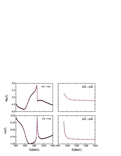
Figure 1: The fits to the $\pi\pi$ and $K\bar{K}$ amplitudes generated from Model I-A(solid black) by using Model I-B (red dashed) and Model I-C(blue dotted). They agree within $1\%$ and hence are not distinguishable.

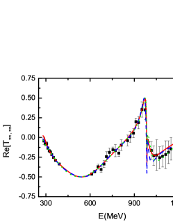
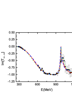
Figure 2: The fits to the empirical $\pi\pi$ amplitude up to 1.2 GeV. The solid red, dashed blue and dotted magenta lines are from using Models II-A, II-B and II-C.

III ANL-Osaka dynamical coupled-channel model and LQCD

The results discussed in section II indicate that in reality the determination of PWA and resonance extraction cannot be performed model independently. It is desirable to investigate nucleon resonances within a reaction model that is constrained by the well-established physics. Thus the meson-exchange mechanisms, which have been well established in the studies of $NN$ scatteringmach and $\pi N$ and $\gamma N$ reactions in the $\Delta$ (1232) regionsl , are used to define the analytic structure of the non-resonant reaction amplitudes in the ANL-Osaka analysis. The results of the ANL-Osaka analysis have been given in detail in Ref.anl-osaka and will not be covered here. Instead, we now turn to explaining how the finite-volume Hamiltonian method developed in Refs.ad-1 ; ad-2 can be applied to relate the ANL-Osaka model Hamiltonian to the LQCD calculations.

In a periodic volume characterized by side length $L$, the quantized three momenta of mesons and baryons must be $k_{n}=\sqrt{n}\frac{2\pi}{L}$ for integers $n=0,1,2,\ldots$. For a given choice of momenta $(k_{0},k_{1},\ldots,k_{N-1})$, solving the Schrodinger equation $(H_{0}+H_{I})|\Psi_{E}\rangle=E|\Psi_{E}\rangle$ in finite volume is equivalent to finding the eigenvalues of the following matrix equations

$$\det([H_{0}]_{N_{c}+1}+[H_{I}]_{N_{c}+1}-E[I]_{N_{c}+1})=0\,,$$ (8)

where $N_{c}=n_{c}\times N$ with $n_{c}$ denoting the number of channels, $[I]_{N_{c}+1}$ is an $(N_{c}+1)\times(N_{c}+1)$ unit matrix. The essence of the finite-volume Hamiltonian method is that the scattering amplitudes calculated from the predicted spectrum by using the Lüscher formulaluch-1 ; luch-2 ; luch-3 are identical to the scattering amplitudes calculated directly from the Hamiltonian in infinite volume. It follows that the spectrum from solving Eq.(8) at any $L$ can be used as the ”data” to test the LQCD calculation at the same $L$, since the information of the nucleon resonances embedded in the data have been coded in the constructed Hamiltonian. No need to perform expensive LQCD calculations covering a wide range of $L$ for investigating the nucleon resonances, such as the Roper $N^{*}(1440)$ resonance, which decay into multi-channel states.

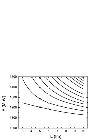
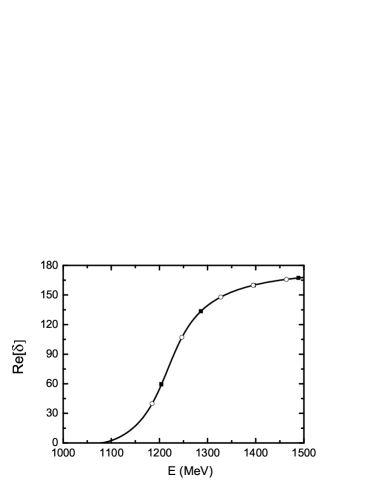
Figure 3: The spectrum (left) and phase shifts (right) in $P_{33}$ state of $\pi N$ system calculated from using the SL modelsl .

The finite-volume Hamiltonian method was established in Ref.ad-1 using a simple one-channel ($n_{c}=1$) Hamiltonian consisting of a $\Delta\rightarrow\pi N$ vertex and a separable $\pi N\rightarrow\pi N$ separable potential. Here we confirm the method by using the meson-exchange model (SL model) of Ref.sl . The results are shown in Fig.3. The predicted energy levels as function of the volume size $L$ are shown in the left-hand side, and the solid curve in the right-hand side is drawn from using the phase shifts calculated from the SL model in infinite volume. For each energy $E$ at a given $L$ in the left-hand side, the Lüscher formula can be used to get the phase shift $\delta(E)$ by

$$\delta(E) = -tan^{-1}(-\frac{q\pi^{3/2}}{Z_{00}(1;q^{2})})+n\pi\,,$$ (9)

where $q=\frac{kL}{2\pi}$ is evaluated by the momentum $k$ defined by $E=E_{N}(k)+E_{\pi}(k)$, and $Z_{00}(1;q^{2})$ is the generalized Zeta function. The phases calculated from each energy at $L=5,6$ in the left-hand side of Fig.3 are the points in the right-hand side, which agree with the solid curve. Thus the finite-volume Hamiltonian method is equivalent to the use of Lüscher formula to relate the spectrum of finite volume to the scattering amplitudes which are obtained from fitting the experimental data through the SL model Hamiltonian.

The Lüscher’s formula for the cases with two open channels, such as that derived in Ref.luch-2 , can be written as

$$\cos\left[\phi(q_{1}(L))+\phi(q_{2}(L))-\delta_{1}-\delta_{2}\right]\quad-\eta\cos\left[\phi(q_{1}(L))-\phi(q_{2}(L))-\delta_{1}+\delta_{2}\right]=0\,,$$ (10)

where $\phi(q_{i}(L)=tan^{-1}(-\frac{q_{i}(L)\pi^{3/2}}{Z_{00}(1;q^{2}_{i}(L))})$ with $q_{i}(L)=\frac{k_{i}(E)L}{2\pi}$, $\delta_{1}(E)$ ($\delta_{2}(E))$ is the phase shifte for channel 1 (2), and $\eta$ is the inelasticity. In the rest frame, this means that we need to perform calculations for three different values of $L$ if Eq.(10) is used to test LQCD results against the data of two phase shifts and inelasicity. On the other hand, the spectrum from finite-volume Hamiltonian method at only one $L$ is sufficient to test LQCD calculations at the same $L$ since the resonances embedded in the data have been coded in the Hamiltonian. Alternatively, one can use the LQCD spectrum to construct a K-matrix model, such as that done in Ref.jlab-lqcd , and then look for the resonance poles. From the results discussed in the previous section, it is clear that such an approach will be reliable only when the predicted phase shifts and inelasticity are of high accuracy and cover a sufficiently wide range of energies such that the parameters of the K-matrix are well conatrained. Thus the LQCD calculations for a wide range of $L$ are required. Here we see the advantage of using the finite volume Hamiltonian method over the use of Lüscher formula to test LQCD calculations.

The ANL-Osaka model Hamiltonian can be schematically written as $H=H_{0}+H_{I}$, where $H_{0}$ is the free Hamiltonian and the interaction Hamiltonian can be written as

$$H_{I}=\sum_{i}\sum_{\alpha}g_{N^{*}_{i},\alpha}+\sum_{M=\rho,\sigma}f_{M,\pi\pi}+\sum_{\alpha,\beta}v_{\alpha,\beta}\,,$$ (11)

where $\alpha,\beta=\pi N,\eta N,K\Lambda,K\Sigma,\pi\pi N(\pi\Delta,\sigma N,\rho N)$, $g_{N^{*}_{i},\alpha}$ defines the decay of the $i$-th bare $N^{*}$ state into channel $\alpha$, $v_{\alpha,\beta}$ denotes the meson-exchange potential between channels $\alpha$ and $\beta$, and $f_{M,\pi\pi}$ describes the decay of meson $M$ into $\pi\pi$. The interactions are determined by fitting very extensive data of $\pi N,\gamma N\rightarrow\pi N,\eta N,K\Lambda,K\Sigma,\pi\pi N$ processes and the nucleon resonances have been extracted. Thus, a LQCD calculation can be related to the nucleon resonances embedded in the $\pi N$ and $\gamma N$ reactions if its predicted spectrum agree with the spectrum calculated from the ANL-Osaka model Hamiltonian by solving Eq.(8) in finite volume.

In the presence of the transitions to $\pi\pi N$ states due to the $\Delta\rightarrow\pi N$ and $\rho,\sigma\rightarrow\pi\pi$ vertex interactions in Eq.(11), it is rather complex to apply the finite-volume Hamiltonian method to the ANL-Osaka Hamiltonian. To compare our approach with the approach using the Lüscher formula, it is sufficient to consider a three-channel Hamiltonian which is deduced from Eq.(11) by keeping only $\pi N$, $\pi\Delta$, and $\sigma N$ channels and neglecting the $f_{\rho,\pi\pi}$ and $f_{\sigma,\pi\pi}$ vertex interactions. We determine this three-channel model Hamiltonian by fitting the $\pi N$ scattering amplitudes up to only $1.6$ GeV. Except the $S_{11}$ partial wave, which is known to have large coupling with the $\eta N$ channel and therefore cannot be fitted well here, the fits are comparable to those of the ANL-Osaka results. The extracted resonance poles are with masses $M_{R}=1353.5\,\,-i\,38.3$ MeV for $P_{11}$ and $M_{R}=1211.9\,\,-i\,52.8$ MeV for $P_{33}$. The value for $P_{33}$ is close to the $M_{R}=1216.4\,\,-i\,50.0$ MeV of SL modelsl . This is consistent with what we have shown in the previous section, since the constructed 3-channel model and the SL model give almost the same fits to $P_{33}$ amplitude data below 1.3 GeV.

For our discussion here, we show in Fig.4 the resulting amplitudes for the $\pi N\rightarrow\pi N,\pi\Delta,\sigma N$ transitions in the $P_{11}$ partial wave. These three amplitudes contain the information determined by the data of $\pi N\rightarrow\pi N,\pi\pi N$ reactions. Thus a LQCD calculation aimed at investigating the Roper $N^{*}(1440)$ should at least be consistent with these three amplitudes, since it is known that the decay width for $N^{*}(1440)\rightarrow\pi\Delta,\sigma N\rightarrow\pi\pi N$ is very large. This can only be achieved by using either the multi-channel Lüscher formulaluch-3 or the finite-volume Hamiltonian method. We now turn to comparing these two different approaches within the three-channel model described above.

For the three-channel model with $n_{c}=3$, the matrix for the free Hamiltonian in Eq.(8) takes the following form

$$[H_{0}]_{3N+1} = \left(\begin{array}[]{cccccccc}m_{0}&0&0&0&0&\cdots\\ 0&E_{\pi}(k_{0})+E_{N}(k_{0})&0&0&0&\cdots\\ 0&0&E_{\pi}(k_{0})+E_{\Delta}(k_{0})&0&0&\cdots\\ 0&0&0&E_{\sigma}(k_{0})+E_{N}(k_{0})&0&\cdots\\ 0&0&0&0&E_{\pi}(k_{1})+E_{N}(k_{1})&\cdots\\ \vdots&\vdots&\vdots&\vdots&\vdots&\ddots\end{array}\right),$$ (18)

where $E_{a}(k)=\sqrt{m_{a}^{2}+k^{2}}$ is the energy of particle $a$ with a mass $m_{a}$, The $(3N+1)\times(3N+1)$ matrix for the interaction Hamiltonian is

$$[H_{I}]_{3N+1} = \left(\begin{array}[]{cccccccc}0&g^{fin}_{\pi N}(k_{0})&g^{fin}_{\pi\Delta}(k_{0})&g^{fin}_{\sigma N}(k_{0})&g^{fin}_{\pi N}(k_{1})&\cdots\\ g^{fin}_{\pi N}(k_{0})&v^{fin}_{\pi N,\pi N}(k_{0},k_{0})&v^{fin}_{\pi N,\pi\Delta}(k_{0},k_{0})&v^{fin}_{\pi N,\sigma N}(k_{0},k_{0})&v^{fin}_{\pi N,\pi N}(k_{0},k_{1})&\cdots\\ g^{fin}_{\pi\Delta}(k_{0})&v^{fin}_{\pi\Delta,\pi N}(k_{0},k_{0})&v^{fin}_{\pi\Delta,\pi\Delta}(k_{0},k_{0})&v^{fin}_{\pi\Delta,\sigma N}(k_{0},k_{0})&v^{fin}_{\pi\Delta,\pi N}(k_{0},k_{1})&\cdots\\ g^{fin}_{\sigma N}(k_{0})&v^{fin}_{\sigma N,\pi\pi}(k_{0},k_{0})&v^{fin}_{\sigma N,\pi\Delta}(k_{0},k_{0})&v^{fin}_{\sigma N,\sigma N}(k_{0},k_{0})&v^{fin}_{\sigma N,\pi N}(k_{0},k_{1})&\cdots\\ g^{fin}_{\pi N}(k_{1})&v^{fin}_{\pi N,\pi N}(k_{1},k_{0})&v^{fin}_{\pi N,\pi\Delta}(k_{1},k_{0})&v^{fin}_{\pi N,\sigma N}(k_{1},k_{0})&v^{fin}_{\pi N,\pi N}(k_{1},k_{1})&\cdots\\ \vdots&\vdots&\vdots&\vdots&\vdots&\ddots\end{array}\right),$$ (25)

with

$$g^{fin}_{\alpha}(k_{n}) = \sqrt{\frac{C_{3}(n)}{4\pi}}\left(\frac{2\pi}{L}\right)^{3/2}g_{N^{*}_{1},\alpha}(k_{n}),$$ (26)

$$v^{fin}_{\alpha,\beta}(k_{n_{i}},k_{n_{j}}) = \sqrt{\frac{C_{3}(n_{i})}{4\pi}}\sqrt{\frac{C_{3}(n_{j})}{4\pi}}\left(\frac{2\pi}{L}\right)^{3}v_{\alpha,\beta}(k_{n_{i}},k_{n_{j}}),$$ (27)

where $C_{3}(n)$ is the number of degenerate states with the same magnitude $k_{n}=|\vec{k}_{n}|$. By solving Eq. (8), we then obtain the spectra for $P_{11}$ shown in Fig. 5.

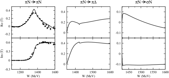
Figure 4: The $\pi N\rightarrow\pi N$ (left), $\pi N\rightarrow\pi\delta$ (middle), and $\pi N\rightarrow\sigma N$ (right) amplitudes for the $P_{11}$ state calculated from the 3-channel model described in the text.

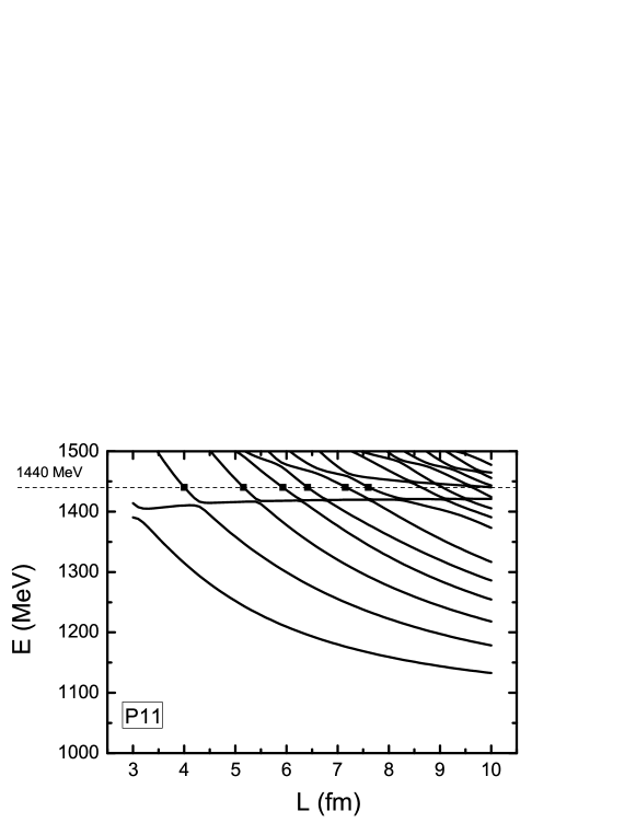
Figure 5: The spectrum for the $P_{11}$ state calculated from from the 3-channel model described in the text.

By choosing the normalization to relate the T-matrix elements to S-matrix elements by $S_{\alpha,\beta}(E)=\delta_{\alpha,\beta}-2iT_{\alpha,\beta}(E)$, the Lüscher formula given in Ref.luch-3 for the constructed 3-channel model can be written explicitly as :

$$\det\left(\begin{array}[]{ccc}T_{\pi N,\pi N}(E)+C_{\pi N,\pi N}(L,E)&T_{\pi N,\pi\Delta}(E)&T_{\pi N,\sigma N}(E)\\ T_{\pi\Delta,\pi N}(E)&T_{\pi\Delta,\pi\Delta}(E)+C_{\pi\Delta,\pi\Delta}(L,E)&T_{\pi\Delta,\sigma N}(E)\\ T_{\sigma N,\pi N}(E)&T_{\sigma N,\pi\Delta}(E)&T_{\sigma N,\sigma N}(E)+C_{\sigma N,\sigma N}(L,E)\end{array}\right)=0\,,$$ (31)

with

$$C_{\alpha,\alpha}(L,E) = iq_{\alpha}(L)/(q_{\alpha}(L)-4\sqrt{\pi}Z_{00}(1;q_{\alpha}(L)),$$ (32)

and $q_{\alpha}(L)=k_{\alpha}L/(2\pi)$ defined by the on-shell momentum $k_{\alpha}$ of the channel $\alpha$.

Because of symmetries and the unitarity conditions, only six of the total 12 real numbers that are needed to specify all of the six complex $T_{\alpha,\beta}(E)$ matrix elements are independent. Thus we need to get six relations from Eqs.(25)-(32) at each $E$ to relate the spectrum to the scattering amplitudes shown in Fig.4 for $P_{11}$. In the rest frame, this means that we need to perform LQCD calculations at 6 different $L$. For $E=1440$ MeV, these are the 6 interaction points (solid squares) between the dashed line and the solid curves in Fig5. Clearly, this will be a very difficult, if not impossible, LQCD calculation. On the other hand, the information on the Roper $N^{*}(1440)$ resonance has been coded in the 3-channel Hamiltonian by fitting the empirical $\pi N$ scattering amplitudessaid as shown in Fig.4. Therefore the spectrum from finite-volume Hamiltonian method at $any$ given L is sufficient to test LQCD calculation. Here we see the great advantage of the finite-volume Hamiltonian method over the approach using the Lüscher formula to test LQCD calculations aimed at investigating the nucleon resonances.

IV Summary

By using several exactly soluble $\pi\pi$ scattering models. we have shown that in reality the determinations of PWA and resonance extractions cannot be performed model independently. It is desirable to extract the nucleon resonances within a reaction model that is constrained by the well-established physics, such as the meson-exchange mechanisms included in the ANL-Osaka and Jüelich analyses.

Within a three-channel model with $\pi N$, $\pi\Delta$ and $\sigma N$ channels, we show the advantage of the finite-volume Hamiltonian method over the approach using the Lüscher formula to test Lattice QCD calculations aimed at investigating the properties of excited nucleon states. To apply the finite-volume Hamiltonian method to predict spectra using the ANL-Osaka dynamical multi-channel Hamiltonian, we need to develop approaches to handle $\pi\pi N$ channels. Since the information on about 25 nucleon resonances with mass up to 2 GeV extracted from the very extensive data of $\pi N,\gamma N\rightarrow\pi N,\eta N,K\Sigma,K\Sigma,\pi\pi N$ reactions have been coded in the ANL-Osaka model Hamiltonian, the predicted spectra can readily be used to test the LQCD calculations aimed at investigating the structure of the excited nucleons. Furthermore, the ANL-Osaka analysis will be applied to include new data from 12 GeV upgrade experiments and thus it will provide more accurate information for testing LQCD calculations in the near future.

- (1) H. Kamano, S.X. Nakamura, T.-S. H. Lee, and T. Sato, Phys. Rev. C 88,035209 (2013).
- (2) A. V. Anisovich, R. Beck, E. Klempt, V. A. Nikonov, A. V. Sarantsev, and U. Thoma, Eur. Phys. J. A 48, 15 (2012).
- (3) D. Ro ̵̈nchen, M. D ̵̈oring, F. Huang, H. Haberzettl, J. Haidenbauer, C. Hanhart, S. Krewald, U.-G. Meissner, and K. Nakayama, Eur. Phys. J. A 49, 44 (2013).
- (4) J. M. M. Hall, A. C.-P. Hsu, D. B. Leinweber, A. W. Thomas and R. D. Young, Phys. Rev. D 87, 094510 (2013).
- (5) Jia-Jun Wu, T.-S.H. Lee, A.W. Thomas, R.D. Young, Phys.Rev. C 90, 055206 (2014)
- (6) R. H. Dalitz and R. G. Moorhouse, Proc. Roy. Soc. Lond. A318, 279 (1970); A. J. F. Siegert, Phys. Rev. 56, 750 (1939). morehouse
- (7) A. Bohm, Quantum mechanics: foundations and applications (Springer-Verlag, New York, 1993).
- (8) W.-T. Chiang and F. Tabakin, Phys. Rev. C 55 (1997) 2054.
- (9) A. M. Sandorfi, S. Hoblit, H. Kamano, and T.-S. H. Lee, J. Phys. G 38, 053001 (2011).
- (10) A. Matsuyama, T. Sato and T. -S. H. Lee, Phys. Rept. 439, 193 (2007)
- (11) R. Machleidt, Chapter 2, Vol.19, Advances in Nuclear Physics, eds. J.W. Negele and E. Vogt, Plenum Press (1989).
- (12) T. Sato and T.-S. H. Lee, Phys. Rev. C 54, 2660 (1996); Phys. Rev. C 63, 055201 (2001).
- (13) M. Lüscher, Nucl. Phys. B 354, 531 (1991).
- (14) S. He, X. Feng and C. Liu, JHEP 0507, 011 (2005)
- (15) M. T. Hansen and S. R. Sharpe, Phys. Rev. D 86, 016007 (2012)
- (16) David J. Wilson, Raul A. Briceno, Jozef J. Dudek, Robert G. Edwards, Christopher E. Thomas, Phys. Rev. D 92, 094502 (2015)
- (17) CNS Data Analysis Center, George Washington University, http://gwdac.phys.gwu.edu