On the Nyström and Column-Sampling Methods for the Approximate Principal Components Analysis of Large Data Sets

Abstract

In this paper we analyze approximate methods for undertaking a principal components analysis (PCA) on large data sets. PCA is a classical dimension reduction method that involves the projection of the data onto the subspace spanned by the leading eigenvectors of the covariance matrix. This projection can be used either for exploratory purposes or as an input for further analysis, e.g. regression. If the data have billions of entries or more, the computational and storage requirements for saving and manipulating the design matrix in fast memory is prohibitive. Recently, the Nyström and column-sampling methods have appeared in the numerical linear algebra community for the randomized approximation of the singular value decomposition of large matrices. However, their utility for statistical applications remains unclear. We compare these approximations theoretically by bounding the distance between the induced subspaces and the desired, but computationally infeasible, PCA subspace. Additionally we show empirically, through simulations and a real data example involving a corpus of emails, the trade-off of approximation accuracy and computational complexity.

Keywords: Big data; Randomized algorithms; Subspace distance.

1 Introduction

In modern statistical applications such as genomics, neural image analysis, or text analysis, the number of covariates $p$ is often extremely large. In this large-$p$ regime, dimension reduction becomes a necessity both for interpretion and for accurate prediction. Though there are numerous methods for reducing the dimensionality of the data — multidimensional scaling, discriminant analysis, locally linear embeddings, Laplacian eigenmaps, and many others — the first, and perhaps the most widely used method, is principal components analysis or PCA (Jollife, 2002).

Suppose our data is $n$ observations, each containing the values of $p$ measurements. Notationally, we represent this as having observations $\tilde{X}_{1},\ldots,\tilde{X}_{n}$, where $\tilde{X}_{i}=(\tilde{X}_{i1},\ldots,\tilde{X}_{ip})^{\top}\in\mathbb{R}^{p}$. After concatenating our data into the matrix $\tilde{\mathbf{X}}=[\tilde{X}_{1},\ldots,\tilde{X}_{n}]^{\top}\in\mathbb{R}^{n\times p}$, we form the matrix $\mathbf{X}$ by centering the columns of $\tilde{\mathbf{X}}$ with the matrix $\overline{\mathbf{X}}=n^{-1}\mathbf{1}\mathbf{1}^{\top}\tilde{\mathbf{X}}$; that is, $\mathbf{X}=\tilde{\mathbf{X}}-\overline{\mathbf{X}}$. Write the (reduced) singular value decomposition (SVD) of $\mathbf{X}$ as

$$\mathbf{X}=U(\mathbf{X})\Lambda(\mathbf{X})V(\mathbf{X})^{\top}=:U\Lambda V^{\top},$$ (1)

where, for any matrix $\mathbf{A}$, we define $U(\mathbf{A})$, $V(\mathbf{A})$, and

$$\Lambda(\mathbf{A})=\textrm{diag}(\lambda_{1}(\mathbf{A}),\ldots,\lambda_{r}(\mathbf{A}))$$ (2)

to be the left and right singular vectors and the singular values of the matrix $\mathbf{A}$, respectively, and $r$ is the rank of $\mathbf{A}$. To simplify notation, we write the singular vectors and values of $\mathbf{X}$ as just $U,V$ and $\Lambda$ and reserve the functional notation for use with other matrices.

For each $d\leq r$, PCA seeks to find a projection that minimizes the squared error distance between the data and the projected data (see e.g. Jollife (2002) for details). These projections are given by the first $d$ columns of $U$ and $V$. For example, if using PCA for regression with response vector $Y$, the fitted values can be written $\widehat{Y}=U_{d}{U_{d}}^{\top}Y$. Here, the notation $\mathbf{A}_{d}$ is the matrix comprised of the first $d$ columns of $\mathbf{A}$ and for $\Lambda_{d}$ we implicitly assume that the vector $(\lambda_{1}(\mathbf{A}),\ldots,\lambda_{r}(\mathbf{A}))$ gets truncated to length $d$ before being transformed into a diagonal matrix as in equation (2).

A Big Problem. For small and medium sized problems in data analysis, PCA provides a powerful method for reducing the dimension of the data via the decomposition in equation (1). However, in modern applications, practitioners are routinely faced with data volumes that seemed unimaginable even a decade ago. In 2000, humans produced 800,000 petabytes of stored data. This number is expected to grow to 35 zettabytes ($3.5\times 10^{22}$ bytes) by 2020. The social media website Twitter.com alone produces 7 terabytes daily (Zikopoulos et al., 2011). In just four hours on “black Friday” 2012, Walmart handled 10 million cash register transactions and sold nearly 5,000 items per second (Wal-Mart Stores, Inc., 2012). Airport security software must handle an arbitrarily large database of high-quality facial images, where each image could have millions of pixels. Storing and processing this data for statistical analysis becomes infeasible even with ever increasing computer technology. These are indications that a practicing, applied statistician should expect to be confronted with very large data sets that need analysis.

For very large problems, PCA encounters two major practical issues: processing constraints and memory constraints. The computational complexity is dominated by the cost of computing the SVD of $\mathbf{X}$, defined in equation (1), which, if $p>n$, is $O(p^{2}n+n^{3})$. If $n$ is rather small, then this computation has quadratic complexity, which can be computationally feasible. However, if $n$ is also very large, say $n\approx p$, then the complexity is $O(n^{3})$, which is infeasible. In addition to the computational cost, there is an irreducible space cost to storing dense matrices in fast memory.

1.1 Approximation Methods

Suppose that $\mathbf{A}\in\mathbb{R}^{q\times q}$ is a symmetric, nonnegative definite matrix with rank $r$; that is, for all $a\in\mathbb{R}^{q}$, $a^{\top}\mathbf{A}a\geq 0$ and $\mathbf{A}^{\top}=\mathbf{A}$. To approximate $\mathbf{A}$, we fix an integer $l\ll q$ and form a sketching matrix $\Phi\in\mathbb{R}^{q\times l}$. Then, we report the following approximation: $\mathbf{A}\approx(\mathbf{A}\Phi)(\Phi^{\top}\mathbf{A}\Phi)^{\dagger}(\mathbf{A}\Phi)^{\top}$. Here, we define $\mathbf{A}^{\dagger}:=V(\mathbf{A})\Lambda(\mathbf{A})^{\dagger}V(\mathbf{A})^{\top}$ to be the Moore-Penrose pseudo inverse of $\mathbf{A}$ with $\Lambda(\mathbf{A})^{\dagger}:=\textrm{diag}(\lambda_{1}(\mathbf{A})^{-1},\ldots,\lambda_{r}(\mathbf{A})^{-1},0,\ldots,0)\in\mathbb{R}^{q\times q}$.

The details behind the formation of the matrix $\Phi$ control the type of approximation. For the Nyström and column-sampling methods, $\Phi=\pi\tau$, where $\pi\in\mathbb{R}^{q\times q}$ is a permutation of the identity matrix and $\tau=[\mathbf{I}_{l},\mathbf{0}]^{\top}\in\mathbb{R}^{q\times l}$ is a truncation matrix with $\mathbf{0}$ the appropriately sized matrix of all zeros. It is important to note that for this particular choice of $\Phi$, we neither explicitly construct $\Phi$ nor form $\mathbf{A}\Phi$. Instead, we can randomly sample $l$ columns of the matrix $\mathbf{A}$ and ignore the rest. Even with other choices of $\Phi$, it is never necessary to store the entire matrix $\mathbf{A}$ in memory as we can read in the rows sequentially to multiply by $\Phi$. Different methods for generating the permutation matrix $\pi$ are available which are discussed in more detail in Section 1.2.

There are alternative methods for choosing $\Phi$ that attempt to approximate the column space of $\mathbf{A}$ by making $\Phi$ a random, dense matrix, such as a subsampled randomized Fourier (or Hadamard) transform or a matrix of i.i.d Gaussians. The product $\mathbf{A}\Phi$ is then post-processed into an orthogonal approximation to $V(\mathbf{A})$. See Halko et al. (2011) or Tropp (2011) for details. Though these techniques are very promising, a joint analysis of these techniques along with the Nyström and column-sampling methods is beyond the scope of this paper and should be addressed in future work.

For sketching matrices $\Phi=\pi\tau$, we can without loss of generality suppose there exists the following block-wise structure to the matrix $\mathbf{A}$

$$\mathbf{A}=\begin{bmatrix}\mathbf{A}_{11}&\mathbf{A}_{21}^{\top}\\ \mathbf{A}_{21}&\mathbf{A}_{22}\\ \end{bmatrix}$$ (3)

such that

$$L(\mathbf{A}):=\mathbf{A}\Phi=\left[\begin{array}[]{c}\mathbf{A}_{11}\\ \mathbf{A}_{21}\\ \end{array}\right]\in\mathbb{R}^{q\times l}.$$ (4)

As $\mathbf{A}_{11}$ is symmetric, we can write its spectral decomposition as

$$\mathbf{A}_{11}=V(\mathbf{A}_{11})\Lambda(\mathbf{A}_{11})V(\mathbf{A}_{11})^{\top}.$$ (5)

The Nyström method. The Nyström method (Williams and Seeger, 2001) uses the matrices $\mathbf{A}_{11}$ and $L(\mathbf{A})$ to compute a low rank approximation to $\mathbf{A}$ via

$$\mathbf{A}\approx L(\mathbf{A})\mathbf{A}_{11}^{\dagger}L(\mathbf{A})^{\top}.$$ (6)

To motivate equation (6), note that

$$L(\mathbf{A})\mathbf{A}^{\dagger}L(\mathbf{A})^{\top}=\left[\begin{array}[]{cc}\mathbf{A}_{11}&V(\mathbf{A}_{11}){V(\mathbf{A}_{11})}^{\top}\mathbf{A}_{21}^{\top}\\ \mathbf{A}_{21}V(\mathbf{A}_{11}){V(\mathbf{A}_{11})}^{\top}&\mathbf{A}_{21}\mathbf{A}_{11}^{\dagger}\mathbf{A}_{21}^{\top}\\ \end{array}\right].$$ (7)

Hence, the Nyström method recovers the $\mathbf{A}_{11}$ entry exactly and a projection of the off diagonal elements.

To facilitate PCA on large data sets, we need to approximate the eigenvectors and eigenvalues of $\mathbf{A}$ rather than attempting to approximate $\mathbf{A}$ itself. The Nyström method can be adapted to this purpose via the simple identity

$$L(\mathbf{A})\mathbf{A}_{11}^{\dagger}L(\mathbf{A})^{\top}=\bigg{(}\kappa_{lq}L(\mathbf{A})V(\mathbf{A}_{11})\Lambda(\mathbf{A}_{11})^{\dagger}\bigg{)}\left(\kappa_{ql}^{2}\Lambda(\mathbf{A}_{11})\right)\bigg{(}\kappa_{lq}L(\mathbf{A})V(\mathbf{A}_{11})\Lambda(\mathbf{A}_{11})^{\dagger}\bigg{)}^{\top},$$ (8)

where for convenience, we define $\kappa_{cd}:=\sqrt{c/d}$ for $c,d\in\mathbb{N}$. These scaling terms are somewhat crude and are intended to compensate for the loss of ‘power’ incurred by subsampling. Hence, we define the Nyström approximation to the eigenvectors of $\mathbf{A}$ to be

$$\kappa_{lq}L(\mathbf{A})V(\mathbf{A}_{11})\Lambda(\mathbf{A}_{11})^{\dagger}=\kappa_{lq}\begin{bmatrix}V(\mathbf{A}_{11})\\ \Omega(\mathbf{A})\end{bmatrix},$$ (9)

where $\Omega(\mathbf{A}):=\mathbf{A}_{21}V(\mathbf{A}_{11})\Lambda(\mathbf{A}_{11})^{\dagger}$, and the Nyström approximation to $\Lambda(\mathbf{A})$ is $\kappa_{ql}^{2}\Lambda(\mathbf{A}_{11})$,

The Column-sampling method. Alternatively, we can operate on the matrix $L(\mathbf{A})$ directly. If we decompose $L(\mathbf{A})$ as

$$L(\mathbf{A})=U(L)\Lambda(L)V(L)^{\top},$$ (10)

where we suppress the dependence of $L$ on $\mathbf{A}$ for clarity, then, analogously to equation (9), the column-sampling approximation to the eigenvectors of $\mathbf{A}$ is

$$L(\mathbf{A})V(L)\Lambda(L)^{\dagger}=U(L).$$ (11)

Likewise, the approximate eigenvalues of $\mathbf{A}$ are given by $\kappa_{ql}\Lambda(L)$.

1.2 Related Work

The Nyström method has recently been used to speed up kernel algorithms in the machine learning community (Drineas and Mahoney, 2005; Belabbas and Wolfe, 2009; Williams and Seeger, 2001; Talwalkar et al., 2008). These works, in contrast with this paper, provide theoretical or empirical bounds on the difference between the kernel matrix and its approximation generated either by the Nyström or column-sampling methods. As the matrices $\mathbf{X}^{\top}\mathbf{X}$ and $\mathbf{X}\mathbf{X}^{\top}$ are both kernel matrices, the bounds derived in these papers apply when performing PCA. However, when using PCA, we are rarely interested in approximating $\mathbf{X}^{\top}\mathbf{X}$.

The sketching matrix $\Phi$ is at the heart of both the Nyström and column-sampling methods, and so, theoretical analysis (for example Zhang et al., 2008; Zhang and Kwok, 2009; Liu et al., 2010; Arcolano and Wolfe, 2010; Kumar et al., 2012; Gittens and Mahoney, 2013) has focused on finding good probability distributions for sampling the columns of $\mathbf{A}$. Several techniques have been proposed, some of the most popular being: uniform sampling, deterministically choosing the columns with largest diagonal entry (e.g. Belabbas and Wolfe, 2009), sampling with probability proportional to $\mathbf{A}_{ii}$ (e.g. Drineas and Mahoney, 2005), or sampling proportionally to the $\ell^{2}$-norms of the eigenvectors known as the leverage scores (e.g. Mahoney, 2011). Leverage scores are much more expensive to compute, although there are some cheap approximations based on power methods. There is little agreement about the benefits of sampling schemes more complicated than the uniform method (see Gittens and Mahoney (2013) for a recent discussion).

We do not consider the effect of choosing different $\pi$ in forming $\Phi$ – that is the effect of different sampling schemes. As both the Nyström and column-sampling methods require the same sketching matrix, we wish to compare these methods post randomization. Hence, our results are conditional on the mechanism that selects the columns. We return to this point in Section 6.

Lastly, an alternate approach to find the SVD is to form an orthonormal basis for a Krylov subspace, which, for a given matrix of interest $\mathbf{X}$, an initial vector $x$, and an iteration parameter $l$, is the column space of $\mathbf{K}_{l}(x)=[x,\mathbf{X}x,\mathbf{X}^{2}x,\ldots,\mathbf{X}^{l-1}x]$. This approach still has a computational complexity of $O((l+s)np)$, where $s$ is an oversampling parameter needed to enhance convergence and hence is more computationally expensive than approaches based on sketches. Additionally, and most seriously, it requires storing the entire matrix $\mathbf{X}$ in fast memory or making repeated calls to slow memory. This requirement rules out the analysis of many interesting, dense data sets.

1.3 Our Contribution

The literature on the Nyström and column-sampling methods centers on making operator or Frobenius norm bounds on the difference between $\mathbf{S}:=n^{-1}\mathbf{X}^{\top}\mathbf{X}$ (or alternatively $\mathbf{Q}:=\mathbf{X}\mathbf{X}^{\top}$) and the approximations $L(\mathbf{S})\mathbf{S}_{11}^{\dagger}L(\mathbf{S})^{\top}$ (Nyström method) or $U(L(\mathbf{S}))\Lambda(L(\mathbf{S}))U(L(\mathbf{S}))^{\top}$ (column-sampling method). While this is important in some cases, PCA-based applications demand techniques and bounds involving the individual matrices of interest $V$, $U$, and $U\Lambda$.

While upper bounds for the distances between these targets and the related approximate quantities can be derived from operator norm (though not Frobenius norm) bounds (Karoui, 2008, for example), such results tend to have at least two problems. First, they are much looser even than the original upper bounds, as operator norm bounds ensure uniform closeness of all unit norm vectors rather than just those desired. Second, letting $V_{nys}$ and $U_{nys}$ be the Nyström approximation to $V$ and $U$, respectively, the previous literature cannot address important questions such as whether $\mathbf{X}V_{nys}$ is a better approximation to $U_{d}\Lambda_{d}$ than $U_{nys}\Lambda_{nys}$, where $\Lambda_{nys}$ approximates $\Lambda$.

In this paper, we produce new bounds for the information loss incurred by a data analyst who wishes to undertake a PCA-based analysis but is forced to perform an approximation using either the Nyström or column-sampling methods. We additionally propose and compare different approximations to $U$ or $V$. These bounds, along with numerical experiments, provide guidance on trading the costs and the computational benefits of these approximation methods in common data analysis scenarios.

2 Approximate PCA

We decompose $\mathbf{X}$ as follows: $\mathbf{x}_{1}=\mathbf{X}\Phi$ and $\mathbf{X}_{1}^{\top}=\mathbf{X}^{\top}\Phi$, $\mathbf{X}=[\mathbf{X}_{1}^{\top},\mathbf{X}_{2}^{\top}]^{\top}=[\mathbf{x}_{1},\mathbf{x}_{2}]$, where $\mathbf{x}_{1}\in\mathbb{R}^{n\times l},\mathbf{x}_{2}\in\mathbb{R}^{n\times(p-l)},\mathbf{X}_{1}\in\mathbb{R}^{l\times p}$, and $\mathbf{X}_{2}\in\mathbb{R}^{(n-l)\times p}$. To approximate $V$ via the Nyström and column-sampling methods, we form $\mathbf{S}:=n^{-1}\mathbf{X}^{\top}\mathbf{X}=n^{-1}V\Lambda^{2}V^{\top}$. Following equations (9) and (11), the Nyström approximation to $V$ is

$$V_{nys}:=\kappa_{lp}L(\mathbf{S})V(\mathbf{S}_{11})\Lambda(\mathbf{S}_{11})^{\dagger}=\kappa_{lp}\begin{bmatrix}V(\mathbf{S}_{11})\\ \Omega(\mathbf{S})\end{bmatrix},$$ (12)

where $\Omega(\mathbf{S})$ is as in equation (9). As $\mathbf{S}=n^{-1}\mathbf{X}^{\top}\mathbf{X}$, we see that $n\mathbf{S}_{11}=\mathbf{x}_{1}^{\top}\mathbf{x}_{1}$ and $nL(\mathbf{S})=\mathbf{X}^{\top}\mathbf{x}_{1}$. Therefore, $V(\mathbf{S}_{11})=V(\mathbf{x}_{1})$ and $n\Lambda(\mathbf{S}_{11})=\Lambda(\mathbf{x}_{1})^{2}$, so that

$$V_{nys} =\kappa_{lp}L(\mathbf{S})V(\mathbf{S}_{11})\Lambda(\mathbf{S}_{11})^{\dagger}$$

$$=\kappa_{lp}\mathbf{X}^{\top}\mathbf{x}_{1}V(\mathbf{x}_{1})\Lambda(\mathbf{x}_{1})^{2\dagger}$$

$$=\kappa_{lp}\mathbf{X}^{\top}U(\mathbf{x}_{1})\Lambda(\mathbf{x}_{1})^{\dagger}$$ (13)

$$=\kappa_{lp}\begin{bmatrix}V(\mathbf{x}_{1})\\ \mathbf{x}_{2}^{\top}U(\mathbf{x}_{1})\Lambda(\mathbf{x}_{1})^{\dagger}\end{bmatrix}$$

and $\Lambda_{nys}=\kappa_{pl}^{2}\Lambda(\mathbf{S}_{11})=n^{-1}\kappa_{pl}^{2}\Lambda(\mathbf{x}_{1})^{2}$. Thus, we can find the Nyström approximation to $V$ by forming $\mathbf{x}_{1}$, calculating its SVD, and then mapping it into the correct space via the adjoint of $\mathbf{X}$. Likewise, the column-sampling approximations to $V$ and $\Lambda$ are

$$V_{cs}:=U(L(\mathbf{S}))\quad\textrm{and}\quad\Lambda_{cs}:=\kappa_{pl}\Lambda(L(\mathbf{S})),$$ (14)

respectively. Here, we see that the column-sampling method orthogonalizes the range of $L(\mathbf{S})$, which is a subset of the range of $\mathbf{S}$.

For approximating $U$, write $\mathbf{Q}=\mathbf{X}\mathbf{X}^{\top}=U\Lambda^{2}U^{\top}\in\mathbb{R}^{n\times n}$, then we can apply the Nyström and column-sampling methods to $\mathbf{Q}$ to approximate $U$. Specifically, writing $\mathbf{Q}_{11}=U(\mathbf{Q}_{11})\Lambda(\mathbf{Q}_{11})U(\mathbf{Q}_{11})^{\top}$,

$$U_{nys}=\kappa_{ln}L(\mathbf{Q})U(\mathbf{Q}_{11})\Lambda(\mathbf{Q}_{11})^{\dagger}\quad\textrm{and}\quad\widetilde{\Lambda}_{nys}=\kappa_{nl}^{2}\Lambda(\mathbf{Q})\\$$ (15)

and the column-sampling approximations are

$$U_{cs}=U(L(\mathbf{Q})),\quad\textrm{and}\quad\widetilde{\Lambda}_{cs}=\kappa_{nl}\Lambda(L(\mathbf{Q})).$$ (16)

However, as $\mathbf{Q}_{11}=\mathbf{X}_{1}\mathbf{X}_{1}^{\top}$ and $L(\mathbf{Q})=\mathbf{X}\mathbf{X}_{1}^{\top}$, we see that approximating $U$ in this manner corresponds to subsampling rows of $\mathbf{X}$, which are the observations. This should be compared to the $V$ approximation case, which corresponds to subsampling columns of $\mathbf{X}$. As the covariates are very likely to be redundant, this should produce a modest approximation error. However, as the observations are not, we are effectively attempting to do inference with large $p$ and smaller $n$ (see Section 4 and Section 5).

To ameliorate this unsavory feature, there are two other possibilities for approximating $U$ that only rely on sampling covariates. First, note that $U=\mathbf{X}V\Lambda(\mathbf{X})^{\dagger}$ and therefore knowing $V$ and $\Lambda(\mathbf{X})$ exactly would allow us to compute $U$ exactly. We can define the following approximations to $U$ based on $V_{nys}$ and $V_{cs}$

$$\widehat{U}_{nys}=\mathbf{X}V_{nys}\Lambda_{nys}^{\dagger/2}$$ (17)

and

$$\widehat{U}_{cs}=\mathbf{X}V_{cs}\Lambda_{cs}^{\dagger/2}.$$ (18)

A second way is to realize that $\textrm{ran}(\mathbf{x}_{1})\subseteq\textrm{ran}(\mathbf{X})$, where $\textrm{ran}(\mathbf{A})$ is the column space (or range) of the matrix $\mathbf{A}$ and the inclusion is equality if the last $p-l$ columns (after permutation) of $\mathbf{X}$ are redundant. Hence, $\mbox{ran}(U(\mathbf{x}_{1}))$ provides a natural approximation to $\mbox{ran}(U)$, suggesting the approximation $\widehat{U}=U(\mathbf{x}_{1})$. See Table 1 for a summary of these approximation methods.

Lastly, we note that approximating the principal components of $\mathbf{X}$ — that is $U\Lambda$ — could be accomplished via any number of approaches such as $U_{nys}\widetilde{\Lambda}_{nys}$, $\mathbf{X}V_{nys}$, $U_{cs}\widetilde{\Lambda}_{cs}$, or $\mathbf{X}V_{cs}$. We do not pursue investigating these approximations directly, rather we investigate approximating $V$ and $U$ as a proxy.

Quantity of interest	Label	Approximations
$V$	$V_{nys}$	$L(\mathbf{S})V(\mathbf{S}_{11})\Lambda(\mathbf{S}_{11})^{\dagger}$
	$V_{cs}$	$U(L(\mathbf{S}))$
	$U_{nys}$	$L(\mathbf{Q})V(\mathbf{Q}_{11})\Lambda(\mathbf{Q}_{11})^{\dagger}$
	$U_{cs}$	$U(L(\mathbf{Q}))$
$U$	$\widehat{U}_{nys}$	$\mathbf{X}V_{nys}\Lambda_{nys}^{\dagger/2}$
	$\widehat{U}_{cs}$	$\mathbf{X}V_{cs}\Lambda_{cs}^{\dagger/2}$
	$\widehat{U}$	$U(\mathbf{x}_{1})$

Table 1: Summary of approximation methods

3 Computations

The Nyström method for approximating $V$ can be computed in a number of ways, based on whether space is a limiting quantity. Two such methods are shown in Algorithm 1 and Algorithm 2. The first uses the matrix $\mathbf{S}_{11}$ while the second does not. In each case, the first step is to form $\mathbf{x}_{1}=\mathbf{X}\Phi$. While computing $\mathbf{X}\Phi$ involves a large matrix multiplication, such a step is unnecessary for either method here. In both cases, we choose a random size $l$ subset of the integers $\{1,\ldots,p\}$ and select these columns of $\mathbf{X}$ to read into memory. For more general $\Phi$, we can sequentially read in rows of $\mathbf{X}$ and multiply by $\Phi$, and hence never read in the entire matrix $\mathbf{X}$.

input : Approximation parameter $l$

Form $\mathbf{x}_{1}$ by randomly selecting $l$ columns of $\mathbf{X}$

Set $\mathbf{S}_{11}=n^{-1}\mathbf{x}_{1}^{\top}\mathbf{x}_{1}$

Compute $V(\mathbf{S}_{11})$ and $\Lambda(\mathbf{S}_{11})$ return $L(\mathbf{S})V(\mathbf{S}_{11})\Lambda(\mathbf{S}_{11})^{\dagger}$

Algorithm 1 Space-efficient computation of $V_{nys}$

input : Approximation parameter $l$

Form $\mathbf{x}_{1}$ by randomly selecting $l$ columns of $\mathbf{X}$

Compute $U(\mathbf{x}_{1})$ and $\Lambda(\mathbf{x}_{1})$ (the left singular vectors and singular values of $\mathbf{x}_{1}$)

return $\mathbf{X}^{\top}U(\mathbf{x}_{1})\Lambda(\mathbf{x}_{1})^{\dagger}$

Algorithm 2 Stable computation of $V_{nys}$

Note that the final steps of both approaches can be performed in a parallelizable way and do not involve reading the entire matrix $\mathbf{X}$ into memory at the same time. Hence, Algorithm 1 requires the storage of only the matrix $\mathbf{S}_{11}$, which has $l^{2}$ entries, while Algorithm 2 requires storing the matrix $\mathbf{x}_{1}$, which has $nl$ entires. Forming $\mathbf{S}_{11}=n^{-1}\mathbf{x}_{1}^{\top}\mathbf{x}_{1}$ and getting its eigenvector decomposition has the same computational complexity as getting $\Lambda(\mathbf{x}_{1})$ and $V(\mathbf{x}_{1})$ directly from $\mathbf{x}_{1}$ (O$(nl^{2}+l^{3})$). If space allows, Algorithm 2 is preferable as it is more stable than Algorithm 1.

Alternatively, the column-sampling method requires forming $L(\mathbf{S})\in\mathbb{R}^{p\times l}$, which has complexity O($lnp$), and its left singular vectors and singular values, which has complexity O($p^{2}l$). For space constraints, Nyström only requires the storage and manipulation of $\mathbf{S}_{11}$, which has $l^{2}$ entries, while column-sampling requires using the $lp$ entries found in $L(\mathbf{S})$. Therefore, there is a substantial savings in both computations and storage when choosing the Nyström method over the column-sampling method. See Table 2 for a summary of these complexities. Lastly, if an approximation to $U$ is desired, $\widehat{U}_{nys}=\mathbf{X}V_{nys}\Lambda_{nys}^{\dagger/2}$ or $\widehat{U}_{cs}=\mathbf{X}V_{cs}\Lambda_{cs}^{\dagger/2}$ can be readily computed via its definition.

A significant advantage of column-sampling over Nyström is that the columns of $V_{cs}$ are orthogonal by virtue of being the left singular vectors of $L(\mathbf{S})$. This imbues column-sampling with better numeric properties and fewer concerns about the meaning of a non-orthogonal approximation to $V$. We could, in principal, orthogonalize $V_{nys}$ to achieve a middle ground between these two methods. However, this orthogonalization step, performed, say, by a QR decomposition has complexity $O(p^{2}l)$, which is of the same order as the singular value decomposition of $L(\mathbf{S})$ and hence would eliminate the computational advantage of choosing the Nyström method over the column-sampling method to begin with.

	Complexity:
Method	Computational	Storage
Nyström	O$(nl^{2}+l^{3})$	O($l^{2}$) [O($nl$)]
column-sampling	O$(lnp+p^{2}l)$	O($pl$)

Table 2: The complexity of the Nyström and column-sampling methods for approximating $V$. The brackets indicate Algorithm 1 and [Algorithm 2]. In particular, the Nyström is only linear in $n$ and $p$ while the column-sampling method is quadratic.

4 Empirical results

Before turning to theoretical guarantees, we present two empirical comparisons of the Nyström and column-sampling methods. The first is a simulation study that explores the approximation accuracy. The second is an analysis of a large corpus of emails sent at the company Enron in the months before its collapse.

4.1 Simulation

Outline. We record four simulation conditions for comparing these approximation methods. In all cases, we draw $n=5000$ observations from a multivariate normal distribution on $\mathbb{R}^{p}$ with zero mean and covariance matrix $\Sigma$, where $p=3000$. We study four different covariance conditions labelled $\textrm{\tt Random}_{0.001}$, $\textrm{\tt Random}_{0.01}$, $\textrm{\tt Random}_{0.1}$, and Band. Here, $\textrm{\tt Random}_{x}$ indicates that, with probability $x$ and for $i<j$, $\Sigma_{ij}^{-1}=1$ and 0 otherwise (diagonal elements are always equal to 1) and $\Sigma^{-1}$ is further symmetrized so that for $j>i$, $\Sigma_{ij}^{-1}$ is set to the same value as $\Sigma_{ji}^{-1}$. Likewise, Band indicates that $\Sigma_{ij}^{-1}=1$ if $|i-j|\leq 50$ and 0 otherwise. For the graph generated by these precision matrices, these simulation conditions result in approximately $\binom{p}{2}\cdot x$ edges for $\textrm{\tt Random}_{x}$ and exactly $25(2p-1-50)$ edges for Band.

For each simulation condition, we consider forming both $V_{d}$ and $U_{d}$ and their respective approximations from Table 1 for a variety of $d$’s. For each $d$, we compute the $d$-dimensional approximation method for 10 equally spaced $l$ values between $3d/2$ and $\min\{15d,2p/5\}$. We record the total computation times (in seconds) in Table 3 and Table 4 for the Nyström and column-sampling methods, respectively. These computations are from R 2.15.3 on an iMac desktop with a 2.9GHz quad-core Intel Core i5 processor and 8 gb of memory. The PCA eigenvectors $V_{d}(S)$ are computed using the package irlba on the $\mathbf{X}$ matrix and we use Algorithm 2 for the Nyström method.

$d$	Approximation parameter ($l$)										$V_{d}(S)$
2	0.4	0.4	0.3	0.3	0.5	0.7	0.8	0.7	0.7	0.7	3.3
3	0.3	0.2	0.3	0.3	0.5	0.7	0.7	0.8	0.8	0.8	4.5
30	1.3	1.1	1.6	1.9	2.0	2.9	2.9	3.8	7.1	12.0	29.6
97	5.0	4.9	7.4	8.3	16.1	19.9	30.2	28.3	36.8	44.3	84.0
164	6.9	7.4	10.4	11.9	16.7	19.7	25.8	30.5	36.7	43.5	117.0
231	9.3	10.9	14.1	16.5	19.5	24.6	27.5	32.6	40.8	45.3	299.0
299	14.2	14.3	19.3	20.2	22.2	26.7	30.8	34.8	40.9	46.6	521.5
366	17.5	18.4	21.2	23.5	37.9	36.8	36.2	39.7	43.0	46.2	791.6
433	20.9	23.0	27.2	31.6	34.0	33.7	39.7	41.2	45.0	49.3	1088.0
500	31.3	30.3	31.6	43.8	45.2	49.9	52.5	54.8	58.4	62.5	1395.3

Table 3: Computing times (in seconds) for the Nyström method, averaged over 4 runs: For each $d$, the approximation parameter, $l$, is on an equally spaced grid of length 10 from $3d/2$ to $\min\{15d,2p/5\}$.

$d$	Approximation parameter ($l$)										$V_{d}(S)$
2	0.7	0.6	0.7	1.0	1.2	1.1	1.3	1.3	1.3	1.5	3.3
3	0.5	0.5	0.6	0.7	0.9	0.8	2.4	1.8	1.1	2.5	4.5
30	4.9	3.1	3.6	7.3	5.9	6.6	7.4	10.2	14.6	12.3	29.6
97	29.5	12.2	20.8	27.9	25.4	36.4	39.7	38.1	42.3	44.6	84.0
164	19.4	33.0	37.6	44.0	57.3	52.6	58.3	65.9	73.6	80.6	117.0
231	42.3	57.0	71.8	80.2	91.4	93.9	102.3	108.2	126.2	131.4	299.0
299	77.0	142.3	119.9	135.3	139.1	146.0	164.0	190.2	186.0	198.2	521.5
366	143.2	155.5	168.0	212.7	227.4	236.1	228.9	231.0	290.2	323.8	791.6
433	220.8	244.1	283.7	303.6	305.4	321.3	355.5	309.1	320.9	346.8	1088.0
500	312.9	351.7	392.5	417.4	426.4	427.9	452.9	418.7	456.4	432.2	1395.3

Table 4: Computing times (in seconds) for the column-sampling method, averaged over 4 runs: For each $d$, the approximation parameter, $l$, is on an equally spaced grid of length 10 from $3d/2$ to $\min\{15d,2p/5\}$.

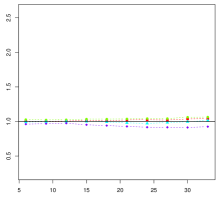
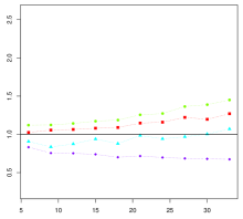
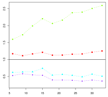
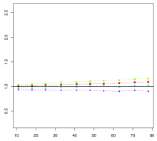
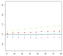
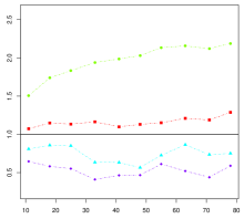
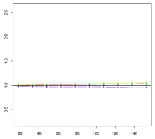
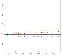
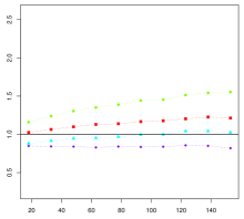
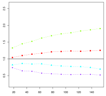
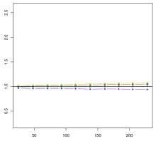
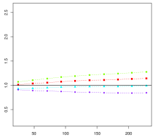
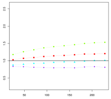
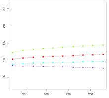
Results. In each of the figures below, we display the accuracy of each approximation method relative to the accuracy of the column-sampling method. Specifically, we report the Frobenius norm error of each method relative to the column-sampling method. For example, for recovering $V_{d}$ with the Nyström method, we plot

$$\frac{||V_{nys,d}({V_{nys,d}}^{\top}V_{nys,d})^{-1}{V_{nys,d}}^{\top}-V_{d}{V_{d}}^{\top}||_{F}}{||V_{cs,d}{V_{cs,d}}^{\top}-V_{d}{V_{d}}^{\top}||_{F}}.$$ (19)

Therefore, larger values indicate inferiority to the column-sampling method and smaller values indicate superiority. We choose the Frobenius norm distance to the PCA-based projection as we are interested in the accuracy loss of using an approximation method instead of the PCA basis.

In Figure 1 we plot a comparison of the Nyström and column-sampling methods when used to approximate $V$. We see that in all cases, the column-sampling performs better than the Nyström method. For small values of $d$, this difference is negligible for $\textrm{\tt Random}_{0.001}$, which is the sparsest case, and increasingly more pronounced for the more dense cases. The banded case demonstrates the largest difference between the Nyström and column-sampling methods, displaying the parabolic relationship between $l$ and approximation error predicted by the theory in Section 5. For larger values of $d$, the banded case displays a phase shift as the benefit of using the column-sampling method over the Nyström method erodes. This curious property is in need of further investigation.

($d=2$)	($d=5$)
($d=10$)	($d=15$)

Figure 1: This figure shows the norm difference of $V_{nys}$ to $V$ relative to the norm difference of $V_{cs}$ to $V$ (see equation (19)) where the $x$-axis is the approximation parameter $l$ whose values range from $\lfloor 3d/2\rfloor$ to $15d$. The four simulation conditions are $\textrm{\tt Random}_{0.001}$ (solid, square), $\textrm{\tt Random}_{0.01}$ (dashed, circle), $\textrm{\tt Random}_{0.1}$ (dotted, triangle), and Band(dot-dash, diamond).

In Figure 2–Figure 5 we plot a comparison of the $U$ approximation methods described in Table 1. For small $d$, there is almost no difference between the 5 methods in the $\textrm{\tt Random}_{0.001}$ and $\textrm{\tt Random}_{0.01}$ cases but a profound difference for the $\textrm{\tt Random}_{0.1}$ and Band cases. As predicted, the “plug-in” estimators $\widehat{U}_{nys}$ and $\widehat{U}_{cs}$ perform better than either $U_{nys}$ or $U_{cs}$. Somewhat surprisingly, the naive approximation $\widehat{U}$ that directly approximates the column space of $\mathbf{X}$ via subsampling performs markedly worse than any of the other approximation methods. This observation has potentially far reaching implications as this is a commonly used “default” method for approximating the spectrum of large matrices (e.g. Bair et al. (2006)).

Figure 2: $d=2$. This figure shows the norm difference between [$U_{nys}$ (red square), $\widehat{U}$ (green circle), $\widehat{U}_{nys}$ (blue triangle), $\widehat{U}_{cs}$ (purple diamond)] and $U$ relative to the norm difference between $U_{cs}$ and $U$ (see equation (19) for an analogous example), where the $x$-axis is the approximation parameter $l$. The four simulation conditions are $\textrm{\tt Random}_{0.001}$, $\textrm{\tt Random}_{0.01}$, $\textrm{\tt Random}_{0.1}$, and Band (from top left to bottom right).

Figure 3: $d=5$. This figure shows the norm difference between [$U_{nys}$ (red square), $\widehat{U}$ (green circle), $\widehat{U}_{nys}$ (blue triangle), $\widehat{U}_{cs}$ (purple diamond)] and $U$ relative to the norm difference between $U_{cs}$ and $U$ (see equation (19) for an analogous example), where the $x$-axis is the approximation parameter $l$. The four simulation conditions are $\textrm{\tt Random}_{0.001}$, $\textrm{\tt Random}_{0.01}$, $\textrm{\tt Random}_{0.1}$, and Band (from top left to bottom right).

Figure 4: $d=10$. This figure shows the norm difference between [$U_{nys}$ (red square), $\widehat{U}$ (green circle), $\widehat{U}_{nys}$ (blue triangle), $\widehat{U}_{cs}$ (purple diamond)] and $U$ relative to the norm difference between $U_{cs}$ and $U$ (see equation (19) for an analogous example), where the $x$-axis is the approximation parameter $l$. The four simulation conditions are $\textrm{\tt Random}_{0.001}$, $\textrm{\tt Random}_{0.01}$, $\textrm{\tt Random}_{0.1}$, and Band (from top left to bottom right).

Figure 5: $d=15$. This figure shows the norm difference between [$U_{nys}$ (red square), $\widehat{U}$ (green circle), $\widehat{U}_{nys}$ (blue triangle), $\widehat{U}_{cs}$ (purple diamond)] and $U$ relative to the norm difference between $U_{cs}$ and $U$ (see equation (19) for an analogous example), where the $x$-axis is the approximation parameter $l$. The four simulation conditions are $\textrm{\tt Random}_{0.001}$, $\textrm{\tt Random}_{0.01}$, $\textrm{\tt Random}_{0.1}$, and Band (from top left to bottom right).

4.2 Enron data

A well known text processing data set is a compilation of emails sent between 158 employees of the energy trading company Enron in the months precipitating its collapse in 2001 (See https://www.cs.cmu.edu/~enron/ for details). After applying standard text preprocessing techniques, the resulting data set contains $n=39,\!861$ documents and $p=28,\!102$ total words recorded as counts in a document-term matrix, $\tilde{\mathbf{X}}$. Frequently, researchers wishing to analyze this matrix would perform latent semantic indexing (LSI), which amounts to computing the leading right singular vectors of the uncentered matrix $\tilde{\mathbf{X}}$. Since $\tilde{\mathbf{X}}$ is sparse, it is possible to store this matrix and perform LSI using sparse matrix handling techniques. While this means that both the Nyström and column-sampling methods are unlikely to be of direct value for text processing, we choose this example for several reasons. First, LSI is an active and evolving field in which singular vectors of the document-term matrix are used to improve document queries and hence the application is very relevant. Second, due to the sparse structure, we can still compute the eigenvectors of this matrix and hence compare the approximations directly. Note that we do not center $\tilde{\mathbf{X}}$ since this would eliminate the sparsity which renders computation of the singular vectors possible and would contrast with the typical analysis. It should be noted, however, that using the Nyström or column-sampling methods would enable centering in practice resulting in an approximation to PCA.

For $d=2,3,50$ we compute and plot the relative error given by equation (19) for the grid of $l$ values $\{100,230,530,1220,1700,2300,2810\}$ (see Figure 6). Interestingly, for each $d$, smaller values of $l$ have both the Nyström and column-sampling method performing rather similarly. For larger values of $l$, the column-sampling method dramatically outperforms the Nyström method, although this advantage appears to erode for larger values of $d$. This indicates that in the large $l$ regime where the Nyström method has a decided computational advantage it also performs markedly worse than the column-sampling method. This behavior is predicted by the theoretical results presented in the next section.

($d=2$)	($d=3$)	($d=50$)

Figure 6: The norm difference for the Enron data of $V_{nys}$ to $V$ relative to the norm difference of $V_{cs}$ to $V$ (see equation (19)). The $x$-axis is the grid of $l$ values $\{100,230,530,1220,1700,2300,2810\}$.

5 Theoretical results

With so many possible approximations, it is natural to ask two questions: (1) what is the cost in approximation accuracy of using the Nyström method over the column-sampling method? and (2) how do the methods for approximating $V$ and $U$ compare to each other?

Comparing eigenvectors to their approximations in the most obvious fashion can lead to difficulties. It is not possible to directly measure the distance between $V_{d}$ and $V_{nys,d}$ or $V_{cs,d}$ because these matrices are not uniquely defined. Each eigenvector and its approximation is only identified up to a sign change. Also, if eigenvalues of $\mathbf{S}$, $\mathbf{Q}$, $\mathbf{S}_{11}$, $\mathbf{Q}_{11}$, or singular values of $L(\mathbf{S})$ or $L(\mathbf{Q})$ are repeated, then the eigenvectors or their approximations are not uniquely defined. Hence, it is cumbersome to compare $V_{d}$ to $V_{nys,d}$ or $V_{cs,d}$ directly via a matrix norm. Even comparing the column spaces of the matrices is not appropriate as, for any orthogonal $\mathbf{O}\in\mathbb{R}^{d\times d}$, $\mbox{ran}(V_{d}\mathbf{O})=\mbox{ran}(V_{d})$. Instead, we compare the subspaces spanned by the eigenvectors $V_{d}$ (or $U_{d}$) and the relevant approximations. This not only provides a coherent metric, but is exactly the relevant quantity for many principal component based applications.

For any two subspaces $\mathcal{G}$ and $\mathcal{H}$ with associated orthogonal projections $\Pi_{\mathcal{G}}$ and $\Pi_{\mathcal{H}}$, we define the distance between $\mathcal{G}$ and $\mathcal{H}$ to be

$$\Delta(\mathcal{G},\mathcal{H})=||\Pi_{\mathcal{G}}-\Pi_{\mathcal{H}}||_{F}.$$ (20)

We will use $\Delta$ as our loss function for examining how well we can recover the PCA generated subspaces given that we are constrained to using an approximation.

Results. Define $\mathcal{V}_{d}:=\mbox{ran}(V_{d})$. Using $V_{nys,d}$ as the Nyström approximation to $V_{d}$, the Nyström approximation of $\mathcal{V}_{d}$ is $\mathcal{V}_{nys,d}=\mbox{ran}(V_{nys,d})$, which has orthogonal projection $V_{nys,d}((V_{nys,d})^{\top}V_{nys,d})^{-1}(V_{nys,d})^{\top}$. Likewise, the column sampling approximation of the subspace $\mathcal{V}_{d}$ is $\mathcal{V}_{cs,d}=\mbox{ran}(V_{cs,d})$, which has orthogonal projection $V_{cs,d}{V_{cs,d}}^{\top}$.

In this section, we provide bounds on the distance between the subspace $\mathcal{V}$ and its Nyström and column-sampling approximations. As an aside, comparing these two approximations to the population-level eigenvectors of $\mathbb{E}[\tilde{X}_{1}\tilde{X}^{\top}_{1}]-\mathbb{E}[\tilde{X}_{1}]\mathbb{E}[\tilde{X}_{1}]^{\top}$ is of interest, as it is possible that $V_{cs}$, for example, might be farther from $V$ than $V_{nys}$ but closer to $V(\mathbb{E}[\tilde{X}_{1}\tilde{X}^{\top}_{1}]-\mathbb{E}[\tilde{X}_{1}]\mathbb{E}[\tilde{X}_{1}]^{\top})$. However, the perspective of this paper is that the data analyst wishes to conduct a principal components analysis but cannot due to computational or size constraints. Therefore, we seek upper bounds on the accuracy loss incurred through a computational approximation.

We write $\mathbf{X}=[X_{1},\ldots,X_{n}]^{\top}=[x_{1},\ldots,x_{p}]$ and define for two matrices $\mathbf{A}^{(1)}$ and $\mathbf{A}^{(2)}$, $\textrm{gap}_{d}\!\left(\mathbf{A}^{(1)},\mathbf{A}^{(2)}\right)=\lambda_{d}(\mathbf{A}^{(1)})-\lambda_{d+1}(\mathbf{A}^{(2)})$. Then we have the following upper bounds, pointwise with respect to the distribution of both $\pi$ and the data.

Theorem 5.1 (Nyström bound).

Suppose that $\textrm{gap}_{d}\!\left(\mathbf{S},\mathbf{S}_{11}\right)=\epsilon$.

$$\Delta(\mathcal{V}_{d},\mathcal{V}_{nys,d}) \leq\frac{\sqrt{2}}{n\epsilon}\left(2\sum_{j=l+1}^{p}\sum_{k=1}^{l}(x_{j}^{\top}x_{k})^{2}+\sum_{j=l+1}^{p}\sum_{k=l+1}^{p}(x_{j}^{\top}x_{k})^{2}\right)^{1/2}$$

$$\qquad\qquad+\sqrt{2}\left(\textrm{trace}\!\left(\Omega_{d}^{\top}(I+\Omega_{d}\Omega_{d}^{\top})^{-1}\Omega_{d}\right)\right)^{1/2},$$

where $\Omega=\mathbf{S}_{21}V(\mathbf{S}_{11})\Lambda(\mathbf{S}_{11})^{\dagger}$.

Theorem 5.2 (Column-sampling bound).

Suppose $\textrm{gap}_{d}\!\left(\mathbf{S},L(\mathbf{S})\right)=\delta$. Then

$$\Delta(\mathcal{V}_{d},\mathcal{V}_{cs,d}) \leq\frac{1}{\delta n}\left(\sum_{j=l+1}^{p}\sum_{k=1}^{l}(x_{j}^{\top}x_{k})^{2}+\sum_{j=l+1}^{p}\sum_{k=l+1}^{p}(x_{j}^{\top}x_{k})^{2}\right)^{1/2}$$

Remark 5.1.

In Theorem 5.1 and 5.2, as the spectral gap ($\epsilon$ or $\delta$) gets smaller, the bound becomes worse. This is analogous to the necessity of a spectral gap for finding an eigenspace for a given matrix $\mathbf{A}$. Suppose $\mathcal{A}_{1}$ and $\lambda_{d}(\mathbf{A})-\lambda_{d+1}(\mathbf{A})=c$, are the $d$-dimensional eigenspace and spectral gap of $\mathbf{A}$, respectively. The computation of $\mathcal{A}_{1}$ becomes unstable as $c\rightarrow 0$, with $c=0$ implying $\mathcal{A}_{1}$ is no longer uniquely defined.

If we assume additional structure on $\mathbf{X}$ we can more directly compare the Nyström and column-sampling methods. Suppose we know, or are willing to impose, some correlation structure on our data, as given by the following condition

Condition 1.

Define the set $\Xi(r,p)=\{j,k:j\neq k\textrm{ and }1\leq j\leq p,r+1\leq k\leq p\}$. Then we say that $\mathbf{X}$ has $\Xi(r,p)$-coherence $C$ if $\;\max_{(j,k)\in\Xi(r,p)}x_{j}^{\top}x_{k}\leq C$.

As $L(\mathbf{S})^{\top}L(\mathbf{S})=\mathbf{S}_{11}^{2}+\mathbf{S}_{21}^{\top}\mathbf{S}_{21}$ is the sum of nonnegative definite matrices, it must hold that, for any $d$, $\lambda_{d}(L(\mathbf{S})^{\top}L(\mathbf{S}))\geq\lambda_{d}(\mathbf{S}_{11}^{2})$, which implies that $\lambda_{d}(L(\mathbf{S}))\geq\lambda_{d}(\mathbf{S}_{11})$ as both are nonnegative. This implies the following inequality and corollary

$$\frac{1}{\textrm{gap}_{d}\!\left(\mathbf{S},\mathbf{S}_{11}\right)}\leq\frac{1}{\textrm{gap}_{d}\!\left(\mathbf{S},L(\mathbf{S})\right)}.$$ (21)

Corollary .

Suppose $\mathbf{X}$ has $\Xi(l,p)$-coherence $C$ and $\textrm{gap}_{d}\!\left(\mathbf{S},L(\mathbf{S})\right)=\delta$. Then

$$\Delta(\mathcal{V}_{d},\mathcal{V}_{nys,d}) \leq C\frac{\sqrt{p^{2}-l^{2}}}{n\delta}+\sqrt{d-\textrm{trace}\!\left((V_{nys,d}^{\top}V_{nys,d})^{-1}\right)},$$

$$\Delta(\mathcal{V}_{d},\mathcal{V}_{cs,d}) \leq C\frac{\sqrt{(p-l)p}}{n\delta}.$$

The usefulness of is that the upper bounds are easier to compare. We pay a penalty for using Nyström over column-sampling that is comprised of two parts. The first can be interpreted as the relative behavior due to the choice of $l$. For fixed $l$, the limit as $p\rightarrow\infty$ is $l/2$, so the difference between the methods is asymptotically constant. Furthermore, in the fixed $p$ scenario in Section 4, the difference is quadratic in $l$. This behavior is illustrated in Figure 7.

Figure 7: The difference $\frac{\sqrt{p^{2}-l^{2}}}{n\delta}-\frac{\sqrt{(p-l)p}}{n\delta}$ as a function of $l$ for $p$ fixed. The $y$-axis is the size of the difference as a percentage of the maximum. The $x$-axis is $l/p$.

For the second term, any rank $d$ orthogonal matrix $\mathbf{O}$ has $\textrm{trace}(\mathbf{O}^{\top}\mathbf{O})=d$. Therefore, we can interpret the second term in the Nyström bound as being a measure of the deviation from orthogonality that is inherent in the Nyström method. Note that the column-sampling method produces an orthogonal approximation and has no such second term. This comparison partially explains the results from the Enron example discussed in Section 4.2. For moderately large $l$ ($10\%$ of $p$ and $\sim 7\%$ of $n$), column-sampling shows improvement over the Nyström method, while for smaller $l$ relative to $n$, the difference is negligible.

For approximating $U$, there are many choices. Not only is there a Nyström versus column-sampling method trade-off, we can either use the approximation via the matrix $\mathbf{Q}$ (that is, $U_{nys}$ or $U_{cs}$), the indirect approximation of $U$ with the weighted coordinates of $\mathbf{X}$ in the basis found by approximating $V$ (that is, $\widehat{U}_{nys}$ or $\widehat{U}_{cs}$), or by directly using the orthogonalization of $\mathbf{x}_{1}$ (that is, $\widehat{U}$). In what follows, we compare the Nyström versions of these approximations.

After some manipulations analogous to equations (12) and (13), we find that

$$U_{nys}=\mathbf{X}V(\mathbf{X}_{1})\Lambda(\mathbf{X}_{1})^{\dagger}\quad\textrm{and}\quad\widehat{U}_{nys}=\mathbf{X}\begin{bmatrix}V(\mathbf{x}_{1})\\ \mathbf{x}_{2}^{\top}U(\mathbf{x}_{1})\Lambda(\mathbf{x}_{1})^{\dagger}\end{bmatrix}\Lambda(\mathbf{x}_{1})^{\dagger}.$$ (22)

If we rewrite equation (22) using

$$\Psi:=\begin{bmatrix}V(\mathbf{x}_{1})\\ \mathbf{x}_{2}^{\top}U(\mathbf{x}_{1})\Lambda(\mathbf{x}_{1})^{\dagger}\end{bmatrix},$$ (23)

we see that $U_{nys}$ and $\widehat{U}_{nys}$ generate subspaces in a related manner:

$$U_{nys}=\left[\mathbf{X}\frac{v_{1}(\mathbf{X}_{1})}{\lambda_{1}(\mathbf{X}_{1})},\ldots,\mathbf{X}\frac{v_{l}(\mathbf{X}_{1})}{\lambda_{l}(\mathbf{X}_{1})}\right]\quad\textrm{and}\quad\widehat{U}_{nys}=\left[\mathbf{X}\frac{\psi_{1}}{\lambda_{1}(\mathbf{x}_{1})},\ldots,\mathbf{X}\frac{\psi_{l}}{\lambda_{l}(\mathbf{x}_{1})}\right],$$ (24)

where $\psi_{j}=[v_{j}(\mathbf{x}_{1})^{\top},(\mathbf{x}_{2}^{\top}u_{j}(\mathbf{x}_{1})/\lambda_{j}(\mathbf{x}_{1}))^{\top}]^{\top}$ is the $j^{th}$ column of $\Psi$. Therefore, these methods are both special cases of Galerkin methods for discretizing an operator in an integral equation. This realization suggests an interesting extension of these methods using different Galerkin bases that warrants further investigation.

Further simplifications can be made:

$$U_{nys} =\begin{bmatrix}U(\mathbf{X}_{1})\\ \mathbf{X}_{2}^{\top}V(\mathbf{X}_{1})\Lambda(\mathbf{X}_{1})^{\dagger}\end{bmatrix}$$ (25)

and

$$\widehat{U}_{nys} =U(\mathbf{x}_{1})+\mathbf{x}_{2}\mathbf{x}_{2}^{\top}U(\mathbf{x}_{1})\Lambda(S_{11})^{\dagger}.$$ (26)

Remembering that $\widehat{U}=U(\mathbf{x}_{1})$, $\widehat{U}_{nys}$ can be seen to be a perturbation of $\widehat{U}$ by the matrix $\mathbf{x}_{2}\mathbf{x}_{2}^{\top}U(\mathbf{x}_{1})\Lambda(S_{11})^{\dagger}$. Supposing that $\mathbf{x}_{1}$ and $\mathbf{x}_{2}$ are orthogonal to each other, then for any vector $x\in\mathbb{R}^{l}$, $||\widehat{U}x||_{2}\leq||\widehat{U}_{nys}x||_{2}$ and hence $\widehat{U}_{nys}$ includes more range space information than $\widehat{U}$ by preserving the part of vectors in $\mbox{ran}(\mathbf{x}_{2})$. Also, $U_{nys}$ needs to be “extended” to $\mathbb{R}^{p}$ by concatenating $U(\mathbf{X}_{1})$ with $\mathbf{X}_{2}^{\top}V(\mathbf{X}_{1})\Lambda(\mathbf{X}_{1})^{\dagger}$ while $\widehat{U}_{nys}$ is already in the “correct” space.

These facts all point to $\widehat{U}_{nys}$ being the better of the three methods. Indeed, the results from Section 4 provide additional evidence for this conclusion.

6 Discussion

For very large problems, PCA requires addressing computational and memory constraints. The computational complexity of PCA is dominated by finding the SVD of $\mathbf{X}$. Hence, some approximations are required to accomplish a PCA-based reduction of a very large data set. In this paper, we investigate the Nyström and column-sampling methods for approximating the eigenvectors of large, dense matrices.

While the results we present are novel and useful, there are a number of potential avenues for further research. A comparison of the subspaces generated by more general matrix sketches (Halko et al., 2011; Tropp, 2011) would be of interest and could provide better guidance for practitioners. Also, in our analysis of the Nyström and column-sampling methods, we ignore the question of how to select the columns of $\mathbf{X}$, sampling them uniformly. However, other results suggest non-uniform sampling will yield better approximations to $\mathbf{X}$. Choices of sampling methods or the use of different sketching matrices represent additional areas for future work.

Lastly, the centering of the matrix $\mathbf{X}$ can be accomplished in a massively parallel fashion using a distributed computing approach such as Map-Reduce. If the vector of column means and the associated number of observations is saved, then the column means can be readily updated if a new observation is recorded. However, recentering would require another pass through each column of the matrix and hence would be quite slow. Adapting these approaches to streaming data requires further research.

References

- (1)
- Arcolano and Wolfe (2010) Arcolano, N., and Wolfe, P. J. (2010), Nyström approximation of Wishart matrices,, in Acoustics Speech and Signal Processing (ICASSP), 2010 IEEE International Conference on, IEEE, pp. 3606–3609.
- Bair et al. (2006) Bair, E., Hastie, T., Paul, D., and Tibshirani, R. (2006), “Prediction by supervised principal components,” Journal of the American Statistical Association, 101(473).
- Belabbas and Wolfe (2009) Belabbas, M., and Wolfe, P. (2009), “Spectral methods in machine learning and new strategies for very large datasets,” Proceedings of the National Academy of Sciences, 106(2), 369.
- Drineas and Mahoney (2005) Drineas, P., and Mahoney, M. (2005), “On the Nyström method for approximating a Gram matrix for improved kernel-based learning,” Journal of Machine Learning Research, 6, 2153–2175.
- Gittens and Mahoney (2013) Gittens, A., and Mahoney, M. (2013), Revisiting the Nystrom method for improved large-scale machine learning,, in Proceedings of the 30th International Conference on Machine Learning (ICML-13), Vol. 28, pp. 567–575.
- Halko et al. (2011) Halko, N., Martinsson, P.-G., and Tropp, J. A. (2011), “Finding structure with randomness: Probabilistic algorithms for constructing approximate matrix decompositions,” SIAM review, 53(2), 217–288.
- Jollife (2002) Jollife, I. (2002), Principal component analysis. Springer Verlag, New York.
- Karoui (2008) Karoui, N. E. (2008), “Operator norm consistent estimation of large-dimensional sparse covariance matrices,” The Annals of Statistics, pp. 2717–2756.
- Kumar et al. (2012) Kumar, S., Mohri, M., and Talwalkar, A. (2012), “Sampling methods for the Nyström method,” The Journal of Machine Learning Research, 98888, 981–1006.
- Liu et al. (2010) Liu, S., Zhang, J., and Sun, K. (2010), “Learning low-rank kernel matrices with column-based methods,” Communications in Statistics: Simulation and Computation, 39(7), 1485–1498.
- Mahoney (2011) Mahoney, M. W. (2011), “Randomized algorithms for matrices and data,” arXiv preprint arXiv:1104.5557, .
- Talwalkar et al. (2008) Talwalkar, A., Kumar, S., and Rowley, H. (2008), Large-scale manifold learning,, in IEEE Conference on Computer Vision and Pattern Recognition, 2008, IEEE.
- Tropp (2011) Tropp, J. A. (2011), “Improved analysis of the subsampled randomized Hadamard transform,” Advances in Adaptive Data Analysis, 3(01n02), 115–126.
- Wal-Mart Stores, Inc. (2012) Wal-Mart Stores, Inc. (2012), “Walmart U.S. Reports Best Ever Black Friday Events [http://news.walmart.com/news-archive/2012/11/23/walmart-us-reports-best-ever-black-friday-events],”.
- Williams and Seeger (2001) Williams, C., and Seeger, M. (2001), Using the Nyström method to speed up kernel machines,, in Advances in Neural Information Processing Systems, Vol. 13.
- Zhang and Kwok (2009) Zhang, K., and Kwok, J. T. (2009), “Density-weighted Nyström method for computing large kernel eigensystems,” Neural Computation, 21(1), 121–146.
- Zhang et al. (2008) Zhang, K., Tsang, I. W., and Kwok, J. T. (2008), Improved Nyström low-rank approximation and error analysis,, in Proceedings of the 25th international conference on Machine learning, ACM, pp. 1232–1239.
- Zikopoulos et al. (2011) Zikopoulos, P., Eaton, C. et al. (2011), Understanding big data: Analytics for enterprise class hadoop and streaming data. McGraw-Hill.